Robust numerical schemes for anisotropic diffusion

problems, a first step for turbulence modeling in

Lagrangian hydrodynamics

Julien Dambrine, Philippe Hoch, Raphael Kuate, Jerome Loheac, Jerome

Metral, Bernard Rebourcet, Lisl Weynans

To cite this version:

Julien Dambrine, Philippe Hoch, Raphael Kuate, Jerome Loheac, Jerome Metral, et al.. Robustnumerical schemes for anisotropic diffusion problems, a first step for turbulence modeling in La-grangian hydrodynamics. ESAIM: Proceedings, EDP Sciences, 2009, CEMRACS 2008 - Mod-elling and Numerical Simulation of Complex Fluids, 28, pp.80-99. <10.1051/proc/2009040>.<inria-00443523>

HAL Id: inria-00443523

https://hal.inria.fr/inria-00443523

Submitted on 29 Dec 2009

HAL is a multi-disciplinary open accessarchive for the deposit and dissemination of sci-entific research documents, whether they are pub-lished or not. The documents may come fromteaching and research institutions in France orabroad, or from public or private research centers.

L’archive ouverte pluridisciplinaire HAL, estdestinee au depot et a la diffusion de documentsscientifiques de niveau recherche, publies ou non,emanant des etablissements d’enseignement et derecherche francais ou etrangers, des laboratoirespublics ou prives.

ESAIM: PROCEEDINGS, Vol. ?, 2009, 1-10

Editors: Will be set by the publisher

ROBUST NUMERICAL SCHEMES FOR ANISOTROPIC DIFFUSION

PROBLEMS, A FIRST STEP FOR TURBULENCE MODELING IN

LAGRANGIAN HYDRODYNAMICS ∗

Julien Dambrine1, Philippe Hoch2, Raphaël Kuate3, Jérôme Lohéac4, Jérôme

Métral2, Bernard Rebourcet2 and Lisl Weynans1

Abstract. Numerous systems of conservation laws are discretized on Lagrangian meshes where cellsnodes move with matter. For complex applications, cells shape or aspect ratio often do not insuresufficient accuracy to provide an acceptable numerical solution and use of ALE technics is necessary.Here we are interested with conduction phenomena depending on velocity derivatives coming fromthe resolution of gas dynamics equations. For that, we propose the study of a mock of second orderturbulent mixing model combining an elliptical part and an hyperbolic kernel. The hyperbolic part isapproximated by finite-volume centered scheme completed by a remapping step see [7]. A major partof this paper is the discretization of the anisotropic parabolic equation on polygonal distorted mesh. Itis based on the scheme described in [9] ensuring the positivity of the numerical solution. We proposean alternative based on the partitioning of polygons in triangles. We show some preliminary results ona weak coupling of hydrodynamics and parabolic equation whose tensor diffusion coefficient dependson Reynolds stresses.

Résumé. De nombreux systèmes de lois de conservation sont intégrés à l’aide du formalisme lagrang-ien où les sommets des mailles voient leurs position varier au cours du temps. La forme des mailles nepermet pas toujours d’assurer une bonne précision du calcul et les techniques ALE sont nécessaires.Nous nous intéressons ici à des phénomènes de conduction dépendant du gradient de vitesse couplésà la dynamique des gaz. Pour cela, nous proposons l’étude d’un simulacre de modèle de mélangeturbulent du second ordre construit pour combiner terme elliptique et noyau hyperbolique. La partiehyperbolique est résolue par des schéma centrés volumes-finis et le remaillage de la phase ALE estcelui décrit dans [7]. Une partie importante de ce papier est la discrétisation de l’équation paraboliqueanisotrope sur maillage polygonal non régulier. Celle-ci s’inspire du schéma dans [9] qui assure lapositivité de la solution numérique. Nous proposons une variante basée sur le découpage en trian-gles des mailles polygonales. Nous montrons quelques résultats préliminaires sur un couplage faiblehydrodynamique et équation parabolique dont le tenseur de diffusion dépend des tensions de Reynolds.

∗ Special thanks to organizers of Cemracs 08: J.B. Apoung, L. Boudin, M. Ismail, S. Martin, B. Maury, C. Misbah, T.

Takahashi1 Université Bordeaux 1 351, cours de la Libération F-33405 Talence cedex, France2 CEA-DAM, DIF, F 91297, Arpajon, France3 Université de Valenciennes, LAMAV, LME. Mont Houy 59313 Valenciennes cedex 9, France4 LJK (Laboratoire Jean Kuntzmann) et LSP (Laboratoire de Spectrométrie Physique) Université Joseph Fourier - BP 53 -38041 Grenoble Cedex 9, France

c© EDP Sciences, SMAI 2009

2 ESAIM: PROCEEDINGS

1. Introduction

The framework is the Lagrangian formalism on unstructured meshes where several fluids are present in theflow. We are interested in the Euler equations of gas dynamics (1.0.1) written below by way of the convectivetime derivative, the other differential operators are related to a fixed cartesian frame.

ρdτ

dt−−→∇ .−→u = 0,

ρd−→u

dt+−→∇p = 0,

ρdE

dt+ ∇.−→pu = 0,

(1.0.1)

where τ = 1/ρ, ρ the density, −→u velocity and E the total energy of the flow anddq

dt:= ∂tq +−→u

−→∇q for arbitrary

scalar function.We particulary want to study some numerical problems arising when these Euler equations of gas dynamics

(1.0.1) are coupled to turbulence to produce dynamic mixing of fluids.The overall problem is the introduction of a second order turbulent mixing model [14]. Because such modelis quite complex and its complete formulation is not necessary for our present study, one defines an algebraicclosure for quantities defining the dynamics of the turbulence (Rij , k, ε, u”, etc...). It corresponds to a stress-strain relation that allows to couple the average flow quantities to a system of unsteady equations for massconcentrations and their turbulent fluxes. The underlying model is linear and depends on coefficients which arecalculated in terms of the purely hydrodynamic splitted Lagrange-ALE step on two-dimensional unstructuredmeshes. This problem requires to consider a turbulent stress tensor and a diffusion term whose coefficient isproportional to this tensor which varies in time and space.When the cells are too distorted, the Lagrangian formalism is no longer reliable with respect to accuracy,consistency and stability and the use of a rezoning process to adjust the grid (Arbitrary-Lagrangian-Eulerian)is necessary. This step allows to obtain a better grid (smoothness, width) in order to improve the numericalaccuracy of the first order (hyperbolic) operator and second order (anisotropic diffusion) operator of the coupledsystem.The mesh adaptation is based on two treatments. The r-adaptation (see [5]) of the moving grid will be done byscalar weights and/or tensors, depending on the physics (velocity, mass concentrations and/or pressures). Theh-adaptation (see [5]) will also reflect the local nature of the flow, and a major point here is the determinationof the best topological cells in a zone to be remeshed, for that we use the approach described in [7] that dealswith arbitrary convex polygonal remeshing. We emphasize that each new extensive unknown (such as density)needs to be defined in such a way that the overall process preserves conservation. A major constraint in ourapproach is to use a positive scheme for the diffusion process to avoid "entropy violation" on arbitrary starshaped polygonal meshes (inside each cell, it exists at least a point x∗ such that any edge e can be joined to x∗

by a segment included in that cell).The paper is organized as followed, in a first section, we explain a modeling that we want to take into accountin our flow. After what we recall the diffusion scheme we have used for simplicial mesh [9] and we presentour approach to take into account arbitrary star shaped polygonal mesh by cutting it in simplices while usingthe scheme described in [9]. Then by way of test problems we show that the numerical order of our procedureapplied on static mesh exceeds one. We also gives results on Lagrange-ALE mesh concerning weak couplingbetween hydrodynamics and turbulence. Finally, in the last section we draw some perspectives of our algorithm.

ESAIM: PROCEEDINGS 3

2. A Reduce Modeling

2.1. Stress-strain relation

Turbulent mixing occurs when fluids of different characteristics are embedded in a highly perturbed flowwhose averaged quantities are described by turbulence modelling. Recent progress in such area leads to secondorder model for the Reynolds stress and hyperbolic heat type equation for mass concentrations. That physicalmechanism allows a better description of the way fluids are distributed in space and provides necessary accurateinformations to improve the equation of state of the mixing state and to compute reaction rates of speciescompounding each of the fluids. The resulting set of equations is known to be tremendously complex anddeserve specific developpement beyond the aim of the present paper. We focus our attention to two distinctbehaviors of the whole modeling:

(1) the hyperbolic part needs special care on a lagrangian grid because: the accuracy is hard to determine,the stability depends directly on the discretization of gradient operator especially when strong shocksoccurs.

(2) the turbulent diffusion process is non uniformly anisotropic and is discretized on non cartesian meshes.

For sake of simplicity we choose to reduce the model to an artificial strain-stress relation that allows toexpress directly a Reynolds stress in proportion to the dynamics of the flow. That impacts momentum andenergy:

ρd−→u

dt+−→∇p + ∇.R = 0,

ρdE

dt+ ∇.−→pu + ∇.R~u = 0.

(2.1.1)

and the governing equation of mass concentration cα of a fluid α:

ρdcα

dt−∇.

(

Cc”ρk

ηR.

−→∇cα

)

. (2.1.2)

More precisely, with:

ε =1

2

[

−→∇−→u +

(−→∇−→u

)T]

d = ε −1

3(∇ · −→u ) Id

(2.1.3)

One defines the Reynolds stress as:

R =2

3ρkI + ρνT d

νT = c2sL

2s

√

d : ε

k =νT

2

csLs, η =

k3/2

csLs

(2.1.4)

cs and Cc” are given coefficients, Ls a characteristic length of the computational domain.

4 ESAIM: PROCEEDINGS

2.2. Diffusion operator

For each fluid α one defines mass concentration cα as the ratio of mass mα of fluid α and total mass of fluids

contained in a control volume: m =∑

γ

mγ . Usual first gradient closure for cα reads:

ρdcα

dt+ ∇.

−→Fα = 0,

−→F α = −Cc”ρ

k

ηR.

−→∇cα,

(2.2.1)

The diffusion coefficient Cc”ρk

ηR is a non-spherical tensor and can be written as Cc”ρ

(csLs)2

νtR (see (2.2.1)

above). Notice, that a simplified version could be to only take into account isotropic diffusion by way of

Trace(

R)

=2

3ρk.

• For the present paper, we will only focus on a weak coupling for which hydrodynamic quantities modifiesthe diffusion tensor but we do not consider that the solution of diffusion influence the hydrodynamics.

• We will not focus on the discretization of the hydrodynamic part and we refer the reader of [7] wherewe use the overall approach and re-use the same code [2].

3. Mathematical framework for scalar diffusion process

This section is devoted to give a framework for the simplified linear anisotropic time dependent problem.For a computational domain Ω ∈ IR2 with ∂Ω = ∂Ωdir ∪

⊕∂Ωneu (neu and dir stand respectively for "Neumann"

and "Dirichlet"):

∂c∂t

−∇.(D(t, x)−→∇c) = 0 in Q := (0, T) × Ω,

c(0, x) = c0(x) in Ω,c(t, x) = cdir(t, x) on (0, T) × ∂Ωdir,

−D(t, x)−→∇c(t, x).n = cneu(t, x) on (0, T) × ∂Ωneu.

(3.0.2)

D is called the diffusion tensor, D is symmetric and positive defined

D(t, x) =

(

α(t, x) β(t, x)β(t, x) γ(t, x)

)

, with

α(t, x) > 0 andα(t, x)γ(t, x) > (β(t, x))2.

(3.0.3)

An important property for the scalar solution in whole space or with the homogeneous Neumann conditioncneu = 0 (or the energy |c2| associated to (3.0.2) with cdir = 0, c(t, .) ∈ H1

0 (Ω)) of physical interest for suchconservative scalar equation is the monotonicity:

u(t = 0, x) ≥ v(t = 0, x) =⇒ ∀t > 0, u(t, x) ≥ v(t, x). (3.0.4)

In whole space, a semi-group approach in L1 see e.g. [3] for conservative translation-invariant equation (Dindependent of x) (3.0.4) gives a maximum principle. For more general case (with boundary condition) seee.g. [6], the solution satisfies the following two conditions:

• Extremal condition see [10]: decay in time of spatial extrema and Maximum Principle (with boundarycondition here):

min (c(s, .), cb) ≤ min c(t, .) ≤ c(t, .) ≤ max c(t, .) ≤ max (c(s, .), cb) . (3.0.5)

where t > s and cb are the boundary values of c over the interval [s,t].

ESAIM: PROCEEDINGS 5

• Positivity condition. This is a special case of (3.0.4) with v(x) ≡ 0 or special case of (3.0.5) withcb ≥ 0 since c ≡ 0 is obviously solution of (3.0.2) with natural boundary condition. Hence, positivitycan be expressed as:

u(0, x) ≥ 0 =⇒ ∀t > 0, u(t, x) ≥ 0. (3.0.6)

For example, for a temperature or mass concentration evolving with respect to an heat equation, thisconstraint is required for a numerical scheme for arbitrary size/shape of the mesh. Positivity is ourminimal requirement throughout this paper.

We can notice that there is an other approach to study continuous solution of fully nonlinear second order scalarPDE see e.g. [1]:

∂u∂t

+ H(t, x, u,∇u,∇2u) = 0 in (0, T) × Ω,

u(x, 0) = u0(x) in Ω, and some boundary condition on (0, T) × ∂Ω.(3.0.7)

The main assumption on H is the so-called ellipticity:

∀(t, x, u, p) H(t, x, u, p, M) ≤ H(t, x, u, p, N) u ∈ IR, p ∈ IR2, M, N ∈ Ssym,2×2 with M ≥ N, (3.0.8)

for which the definition of a solution (called viscosity-solution) is directly formulated under a maximum principle.A function u is called a viscosity solution of (3.0.7) if and only if it is:

• Sub-solution: ∀Φ(t, x) ∈ C2(Q) if for all local maximum (t∗, x∗) of u − Φ:

∂tΦ(t∗, x∗) + H(t∗, x∗, u(t∗, x∗),∇Φ(t∗, x∗),∇2Φ(t∗, x∗)) ≤ 0, (3.0.9)

• Super-solution: ∀Φ(t, x) ∈ C2(Q) if for all local minimum (t∗, x∗) of u − Φ:

∂tΦ(t∗, x∗) + H(t∗, x∗, u(t∗, x∗),∇Φ(t∗, x∗),∇2Φ(t∗, x∗)) ≥ 0. (3.0.10)

Note that this definition is implicit with respect to extremal points, and that it is not obvious to take it intoaccount directly inside a finite volume scheme. But we mention it for the study of parabolic equations moregeneral than (3.0.2).

4. Properties for discrete numerical scheme

In the spirit of [10] and to mimic (3.0.5), we want to impose the following property to the solution of (3.0.2)in case of implicit scheme with n the time step number, K the mesh element:

min

cn+1K′ , K ′ ∈ V (K)

, cnK , cb

≤ cn+1K ≤ max

cn+1K′ , K ′ ∈ V (K)

, cnK , cb

(4.0.11)

where V(K) is the neighborhood of cells sharing at least a node with cell K, cb is the solution at boundarybetween time [tn, tn+1].Ideally, in our context we want a diffusion scheme that fulfils the following properties:

1 locally conservative.2 consistent and convergent.3 discrete maximum/minimum principle or the weaker positivity condition (3.0.6).4 reliability on arbitrary convex polygonal cells 1 with high aspect ratio and/or cells stretching.5 compatible with heterogeneous and arbitrary anisotropic diffusion tensor (positive defined matrix).

1thanks to ALE and adaptation we suppose that we are able to obtain such mesh, see [7].

6 ESAIM: PROCEEDINGS

Many of these constraints have been taken into account in the paper [9] (see also [11] [15] for related results) butconvergence has to be studied with respect to robustness. We recall their scheme in section 4.1.1 and explainour variant for polygonal cells in the next section 4.1.2.

4.1. Positive solution for a diffusion problem with finite volume approximation

4.1.1. Positive solution of scheme [9] on simplicial mesh with arbitrary diffusion tensor

We recall that the non-linear scheme of [9] corrects [11] in the case of general diffusion tensor. Integratingthe equation (3.0.2) over a triangle T and using Green Formula, we obtain the evolution for the mean value:

∂tcT +1

|T |

∫

∂T

q.nds = 0, q := −D∇c (4.1.1)

and so the following balance:

∂tcT +1

|T |

∑

e∈∂T

qe.ne = 0, ne outward normal of e(T) of length |ne| = |e|. (4.1.2)

Using notation cT instead of cT , we use an implicit time stepping with time step ∆t:

cn+1T +

∆t

|T |

∑

e∈∂T

qn+1e .ne = cn

T (4.1.3)

A two point flux approximation is considered: qe (we omit the time dependence knowing it is implicit), foreach cell T, only one degree of freedom is used and is noted cT (corresponding to cT ) . Hence, a two-point fluxapproximation uses only two degrees of freedom cT+ and cT− (in short c+, c−) per each edge e (see Figure 1):

qe.ne = A+e c+ − A−

e c− (4.1.4)

where coefficients A±e characterizes the scheme and depends on unknowns c itself as we will see. In the con-

struction, there are mainly three steps:

• Step 1 - Definition of the unique collocation point xT in each simplex T.

Let v1, v2, v3 be the vertices, the intersection of the three D-bisector lines defined the collocation point:

xT =

3∑

i=1

viλi, λi =|eθi

|D

∑3j=1 |ej |D

, where |e|D

:= |D1/2

e|. (4.1.5)

Here eθidenotes the edge opposite to vertex vi, hence cT represent now the value of c at xT .

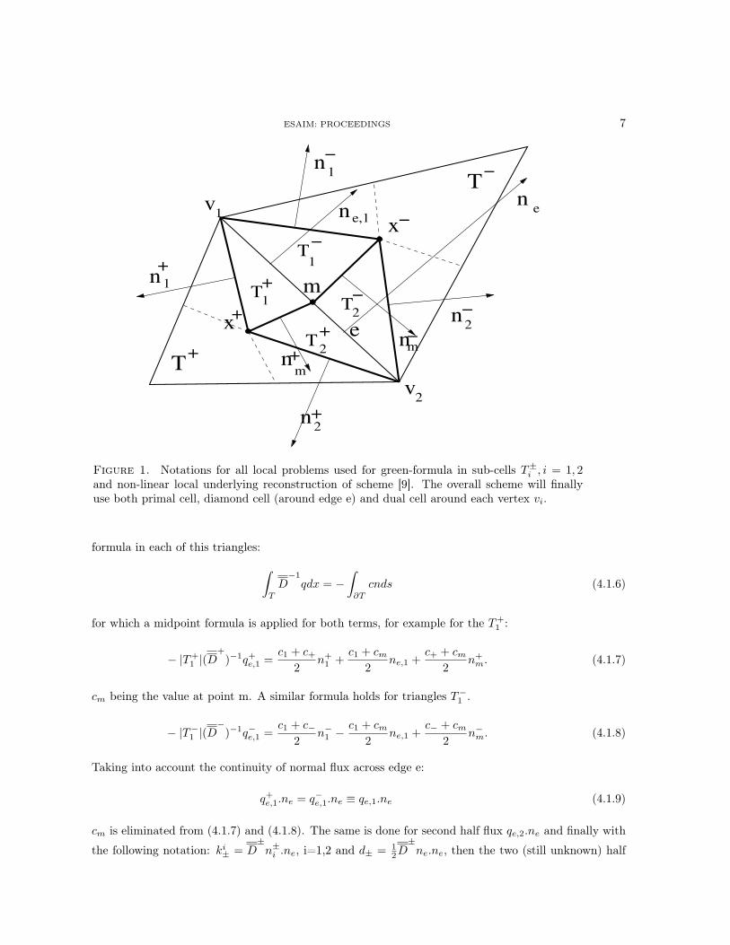
• Step 2 - Local non-linear diamond scheme (half edge flux qe,i, i = 1, 2 computed by local Green formulasand non-linear interpolation):For an interior edge e, m is defined as the midpoint. Let consider T+, T− the two triangles sharing e

and D+

(resp. D−

) the constant metric tensor in T+ (resp. T−) (D+

and D−

are not supposed tobe equal). The two collocations points are denoted by x+, x−. The edge e and the midpoint m splitthe quadrilateral v1x

+v2x− (the diamond cells) into four triangles T±

i , i = 1, 2 see Figure 1. The localnormal vector n±

m and ne,i, i = 1, 2 are the normal to intervals [m;x±] and [m; vi], i = 1, 2. Their lengthis assumed to be equal to the length of the underlying intervals, hence for example: n+

m = |x+ − m|and then ne,i = 1

2ne. Hence, we get the following identity n±1 + n±

m + 12ne = 0. Now applying a Green

ESAIM: PROCEEDINGS 7

x−

T

T

+

−

e

v

v1

2

mT1

T1

T+2

−

n

n

n

n

1

1

2

2

+

−

+

+

−T2

−

n+m

mn−

nen e,1

+x

Figure 1. Notations for all local problems used for green-formula in sub-cells T±i , i = 1, 2

and non-linear local underlying reconstruction of scheme [9]. The overall scheme will finallyuse both primal cell, diamond cell (around edge e) and dual cell around each vertex vi.

formula in each of this triangles:

∫

T

D−1

qdx = −

∫

∂T

cnds (4.1.6)

for which a midpoint formula is applied for both terms, for example for the T+1 :

− |T+1 |(D

+)−1q+

e,1 =c1 + c+

2n+

1 +c1 + cm

2ne,1 +

c+ + cm

2n+

m. (4.1.7)

cm being the value at point m. A similar formula holds for triangles T−1 .

− |T−1 |(D

−)−1q−e,1 =

c1 + c−2

n−1 −

c1 + cm

2ne,1 +

c− + cm

2n−

m. (4.1.8)

Taking into account the continuity of normal flux across edge e:

q+e,1.ne = q−e,1.ne ≡ qe,1.ne (4.1.9)

cm is eliminated from (4.1.7) and (4.1.8). The same is done for second half flux qe,2.ne and finally with

the following notation: ki± = D

±n±

i .ne, i=1,2 and d± = 12D

±ne.ne, then the two (still unknown) half

8 ESAIM: PROCEEDINGS

flux writes:

qe,1.ne =c+d+k1

− + c−d−k1+ − c1(d+k1

− + d−k1+)

2(|T+1 |k1

− − |T−1 |k1

+)

qe,2.ne =c+d+k2

− + c−d−k2+ − c2(d+k2

− + d−k2+)

2(|T+2 |k2

− − |T−2 |k2

+)

(4.1.10)

and a convex combination of this two half fluxes is considered:

qe.ne = µ1qe,1.ne + µ2qe,2.ne, µ1 + µ2 = 1. (4.1.11)

If it verifies a two point flux approximation qe.ne = A+e (c)c+ − A−

e (c)c−, so the resulting solution of(4.1.10) (4.1.11) for internal edges:

A+e (c) = µ1

d+k1−

2(|T+1 |k1

− − |T−1 |k1

+)+ µ2

d+k2−

2(|T+2 |k2

− − |T−2 |k2

+)

−A−e (c) = µ1

d−k1+

2(|T+1 |k1

− − |T−1 |k1

+)+ µ2

d−k2+

2(|T+2 |k2

− − |T−2 |k2

+)

(4.1.12)

where µ1 =γ2

γ2 − γ1, µ2 =

−γ1

γ2 − γ1, with γi =

ci(d+ki− + d−ki

+)

2(|T+i |ki

− − |T−i |ki

+)

For boundary edges:– On ∂Ωdir is imposed Dirichlet boundary condition c = cdir, the flux writes qe.ne = A+

e (c)c++A−e (c)

where:

A+e (c) = − 1

2|T+| (n+1 + n+

2 ).D+ne,

A−e (c) = 1

2|T+| (cdir(v1)n

+2 + cdir(v2)n

+1 ).D

+ne.

(4.1.13)

– On ∂Ωneu, we impose Neumann boundary condition −D∇c.n = cneu, the flux writes:

qe.ne = cneue |ne|. (4.1.14)

where cneue is a mean of cneu on edge e.

• Step 3 - Interpolation of vertex values ci, i = 1, 2 in non-linear flux (4.1.12). In [9], the authors testedthe good behavior of the inverse distance weighting [13] of unknown values c(xT ) for all T around eachvi, let N(vi) be this set. They claimed that interpolation is robust in case of non smooth solution butdid not prove its second order accuracy.

ci =∑

T∈N(vi)

c(xT )wT , wT =|xT − vi|

−1

∑

T ′∈N(vi)|xT ′ − vi|−1

(4.1.15)

The non-linear system discretizing (4.1.3) with boundary condition (4.1.13) (4.1.14) is then M(X)X = b,where:

(1) the matrix M(X) of the discretization for the evolution equation writes:

M(X) := I + Diag(∆t

|T |)A(X), where Diag(

∆t

|T |)ij =

∆t

|Ti|δij (4.1.16)

ESAIM: PROCEEDINGS 9

and ∆t is the time step of Lagrangian step, |T | surface of simplex T, and A(X) the assembling matrixresulting of internal edges (4.1.12) and contributing part of Dirichlet boundary condition A+

e (c) in(4.1.13).

(2) The right hand side b is such that each component (for each simplex):

bT = cnT −

∆t

|T |

(

∑

e∈∂Ωdir∩∂T

A−e +

∑

e∈∂Ωneu∩∂T

cneue |ne|

)

. (4.1.17)

The overall non-linear system M(X)X = b is solved by Picard iteration:

X0 = X∗ such that X∗T ≥ 0,

Solve M(Xk−1)Xk = b, until :||M(Xk)Xk − b|| ≤ ǫnon||M(X0)X0 − b||, (ǫnon = 10−10 if nothing specified)

(4.1.18)

Here, we choose to solve linear systems in (4.1.18) with GMRES algorithm with diagonal preconditioning. It-erations are terminated when relative norm w.r.t initial residual is lower that 10−14.

In [9], for stationary version of (3.0.2) (Poisson equation −∇.D∇u = f so that M(X) is replaced by A(X) in(4.1.16), and cn

T by fK in (4.1.17)), it is proved the following when (4.1.11)(4.1.12)(4.1.18) are used:

Properties 4.1. Let bT ≥ 0, X∗T ≥ 0, for all T, and linear systems in Picard iterations are solved exactly, then

all iterates Xk in (4.1.18) verifies:

XkT ≥ 0, for all T. (4.1.19)

Unfortunately the scheme does not verifies a Discrete Maximum Principle so that overshoot/undershoot oroscillations can appear in numerical solution (see [9] and in section 5.2).

4.1.2. Positive solution on arbitrary convex polygonal mesh by cutting in triangles

The overall scheme [9] does not behave so good if the mesh is composed of arbitrary polygonals, specially forstretched polygonal cells. The reason invoked is partially due to the fact that the construction of a collocationpoint ensuring the system to be positive is only limited to a restricted class of meshes and diffusion tensors. Inour case, the constraint on diffusion tensor can be too strong (we do not control coefficients of the tensor) andour polygonal cells can be both stretched and may be constituted by more than four vertices (see numericalexamples below). A study of how to adapt the mesh and obtain the collocation point such that it ensurespositivity, is far from beeing an easy task. So that for the paper, we finally adopt the strategy that slices thearbitrary polygonal mesh into simplices. This is a sufficient operation that permits to deal with arbitraryanisotropic diffusion coefficient and any star shaped (and then convex) polygonal cells.In brief, we do the following (see Figure 2):

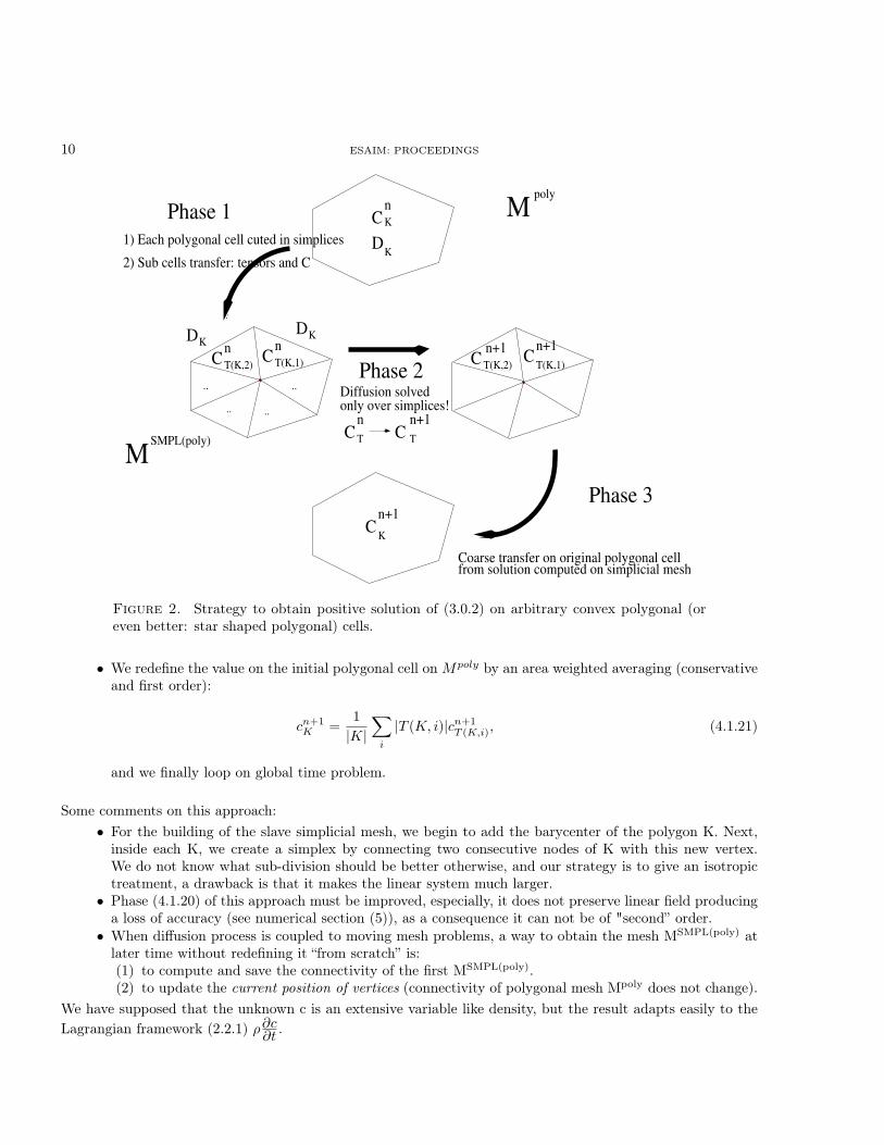
• Let Mpoly be an arbitrary convex polygonal mesh. For any cell K having more than three vertices wesplit it into simplices T (K, i), i ≤ card(K), card(K) the number of vertices in K. Each simplex is definedby two consecutive vertices linked to the gravity center of K (or a point for which the polygonal cellis star shaped), see Phase 1 in Figure 2. We note MSMPL(poly) the resulting mesh constituted by onlytriangles. We transfer all quantities on the splitted triangle cells in a conservative way, at this moment,we only apply a first order transfer:

cnT (K,i) = cn

K , ∀ i = 1, ..., card(K). (4.1.20)

• We solve the diffusion problem with the scheme presented in the previous subsection (4.1.11)(4.1.12)(4.1.18)on the mesh MSMPL(poly), see Phase 2 in Figure 2, so that we get cn+1

T (K,i) on MSMPL(poly).

10 ESAIM: PROCEEDINGS

1) Each polygonal cell cuted in simplices

C

D

K

K

..

.. ..

..

D DKK

n

2) Sub cells transfer: tensors and C

CK

CnT(K,2)

CnT(K,1) C

n+1T(K,2)

Cn+1

T(K,1)

only over simplices!Diffusion solved

C T

nC T

n+1

Coarse transfer on original polygonal cell

n+1

M

M

poly

SMPL(poly)

from solution computed on simplicial mesh

Phase 1

Phase 2

Phase 3

Figure 2. Strategy to obtain positive solution of (3.0.2) on arbitrary convex polygonal (oreven better: star shaped polygonal) cells.

• We redefine the value on the initial polygonal cell on Mpoly by an area weighted averaging (conservativeand first order):

cn+1K =

1

|K|

∑

i

|T (K, i)|cn+1T (K,i), (4.1.21)

and we finally loop on global time problem.

Some comments on this approach:

• For the building of the slave simplicial mesh, we begin to add the barycenter of the polygon K. Next,inside each K, we create a simplex by connecting two consecutive nodes of K with this new vertex.We do not know what sub-division should be better otherwise, and our strategy is to give an isotropictreatment, a drawback is that it makes the linear system much larger.

• Phase (4.1.20) of this approach must be improved, especially, it does not preserve linear field producinga loss of accuracy (see numerical section (5)), as a consequence it can not be of "second” order.

• When diffusion process is coupled to moving mesh problems, a way to obtain the mesh MSMPL(poly) atlater time without redefining it “from scratch” is:(1) to compute and save the connectivity of the first MSMPL(poly).(2) to update the current position of vertices (connectivity of polygonal mesh Mpoly does not change).

We have supposed that the unknown c is an extensive variable like density, but the result adapts easily to the

Lagrangian framework (2.2.1) ρ∂c∂t

.

ESAIM: PROCEEDINGS 11

4.2. Positive solutions for a diffusion problem with linear finite element approximation

Let Ω be a bounded open set of R2, T > 0 and D a symmetric positive definite matrix. We use standard

Sobolev spaces and notations. We want to find u such that:

∂u∂t

−∇ · D∇u = 0 in (0, T) × Ω,

u(x, 0) = U0(x) in Ω, and some boundary condition on (0, T) × ∂Ω.

Let ϕ ∈ H10 (Ω) be a test function. Consider Neumann homogeneous boundary conditions. The classical weak

formulation of the previous problem yields: consider U0 ∈ L2(Ω) and find u ∈ L2(]0, T[;H10 (Ω))∩C([0, T];L2(Ω))

such that:

∫

Ω

∂u

∂tϕ +

∫

Ω

D∇u · ∇ϕ = 0 in (0, T) × Ω,

u(x, 0) = U0(x) in Ω.(4.2.1)

Consider a triangulation Th, h > 0, of Ω and the standard discrete formulation of 4.2.1 using piecewise linear(P1) finite elements discretization. As it is known, the finite element approximation of diffusion problem doesnot always satisfy the maximum principle [4]. We are looking for sufficient conditions for positive solutions ofproblem (4.2.1) with respect to any given positive U0. We use an implicit time step discretization. Let ∆t bethe time step. Let T be a triangle, |T | its area and vi, vj , vk its vertices.

Proposition 4.1. For any positive U0, the P1 finite element approximation of the solution of (4.2.1) is positiveif we have the following conditions:

(D(−−→vkvi)⊥) · (−−→vkvj)

⊥ > 0.

∆t ≥|T |2

6(D(−−→vkvi)⊥) · (−−→vkvj)

⊥.

(4.2.2)

Where (−−→vkvj)⊥ is the external normal to vector −−→vkvj on T .

Proof. Let φi the nodal bases function associated with vi i.e., the continuous piecewise linear finite elementfunction which equals 1 at the vertex vi and which vanishes at all other vertices of Th. Discrete formulation of(4.2.1) yields:

∑

T∈Th

∫

T

(

N∑

i=1

un+1i φiφj + ∆t(D

N∑

i=1

un+1i ∇φi) · ∇φj

)

=∑

T∈Th

∫

T

N∑

i=1

uni φiφj , j = 1, ..., N

Where N is the number of degrees of freedom of Th.

(4.2.3)

Let Ax = b be the linear system obtained from (4.2.3). We want positive solutions of that system. The right-hand side of (4.2.3) is always positive when un

i is positive, so the vector b has non-negative components. A veryuseful characterization of the matrix A in this case is an M-matrix. In [12] page 30, we have a characterizationof an M-matrix A:

• Every diagonal entry of A is positive: true in our case.• Every off-diagonal entry of A is non-positive:

if we look at this statement per triangle, then it is sufficient that

∫

T

φiφj + ∆t(D∇φi) · ∇φj ≤ 0. (4.2.4)

12 ESAIM: PROCEEDINGS

To satisfy (4.2.4) as ∆t > 0, the calculus of ∇φl,l=i,j. and integration on T gives the following sufficientcondition:

∆t ≥|T |2

6(D(−−→vkvi)⊥) · (−−→vkvj)⊥,

(D(−−→vkvi)⊥) · (−−→vkvj)

⊥ > 0.

(4.2.5)

When D is the identity matrix we have classical geometrical conditions on the three angles of T , see [4]:for each angle θ of T , θ ≤ π

2 + ǫ, ǫ > 0.• A have positive row sums:

if we look once more at this last statement per triangle, we obtain:

∫

T

∑

j

(φiφj + ∆t(D∇φi) · ∇φj) > 0.

The sum of the gradients of the nodal basis functions is always null on a triangle then,

∫

T

∑

j

∇φj = 0.

So, the previous inequality gives

∫

T

φ2i > −

∫

T

∑

j 6=i

(φiφj),

which is always true.

ESAIM: PROCEEDINGS 13

5. Tests on purely diffusion process on splitted static mesh

Here, we test the scheme (4.1.11) (4.1.12) (4.1.18) used with the strategy (4.1.20) (4.1.21) for two test cases,the first one on cartesian grid and the second one on a Kershaw like mesh (see [8]).

5.1. Accuracy tests

We investigate the following problem:

∂tc = ∆c in Ω = (0, 1) × (0, 1),

c = 1 on ∂Ω,(5.1.1)

with the initial condition: c0(x) = sin(πx)sin(πy) + 1. The exact solution reads:

cex(t, x) = e−2π2tsin(πx)sin(πy) + 1. (5.1.2)

In the two following test cases, we always take nx = ny for the original cartesian grid (after which we can movethe node to create non uniform quadrilaterals) and we note h = (maxK |K|)1/2 the characteristic mesh spacing(valid for any polygonal mesh), the time step being equals to ∆t = h2. We compute the error by the formulaon the original non splitted mesh e(tn) =

∑

K |K||cex(tn, x∗K) − cn

K |, where x∗K is the gravity center of cell

K and cnK is the solution on the initial polygonal mesh, and we stop at final time T=0.1.

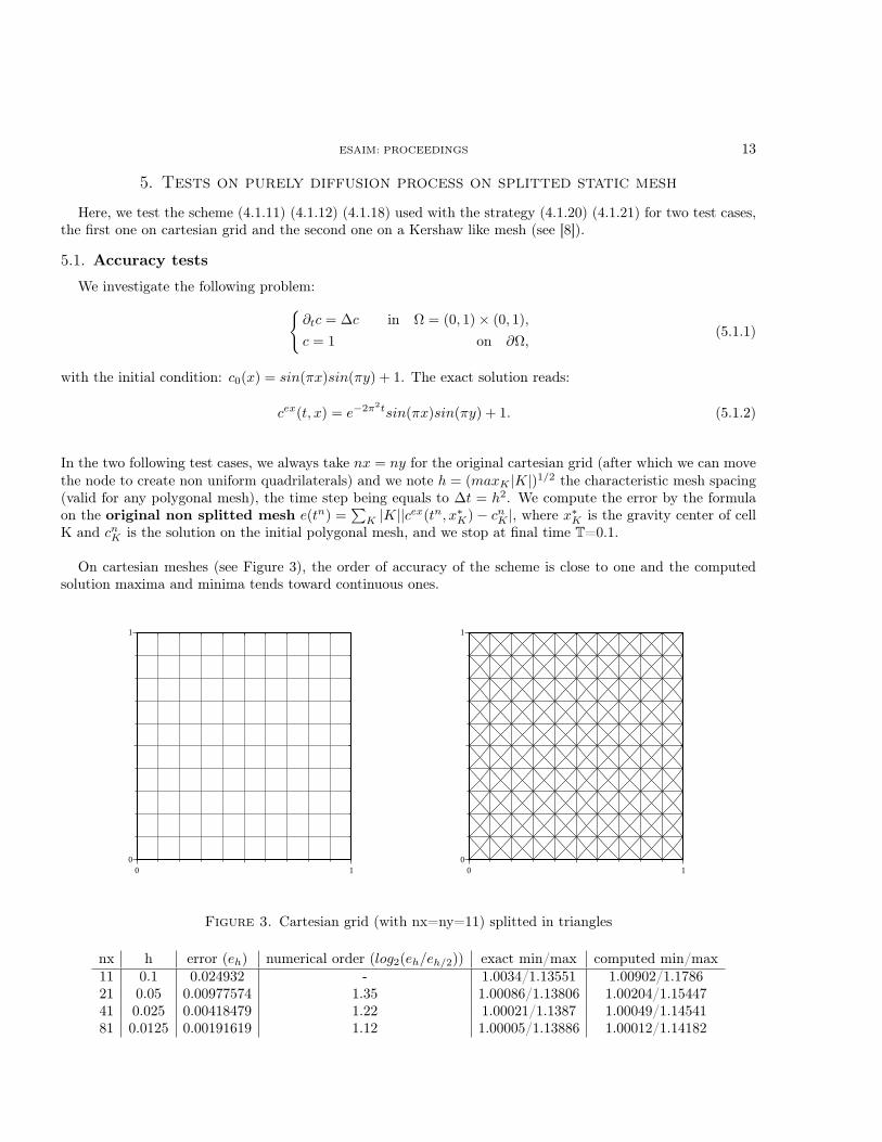
On cartesian meshes (see Figure 3), the order of accuracy of the scheme is close to one and the computedsolution maxima and minima tends toward continuous ones.

0 10

1

0 10

1

Figure 3. Cartesian grid (with nx=ny=11) splitted in triangles

nx h error (eh) numerical order (log2(eh/eh/2)) exact min/max computed min/max11 0.1 0.024932 - 1.0034/1.13551 1.00902/1.178621 0.05 0.00977574 1.35 1.00086/1.13806 1.00204/1.1544741 0.025 0.00418479 1.22 1.00021/1.1387 1.00049/1.1454181 0.0125 0.00191619 1.12 1.00005/1.13886 1.00012/1.14182

14 ESAIM: PROCEEDINGS

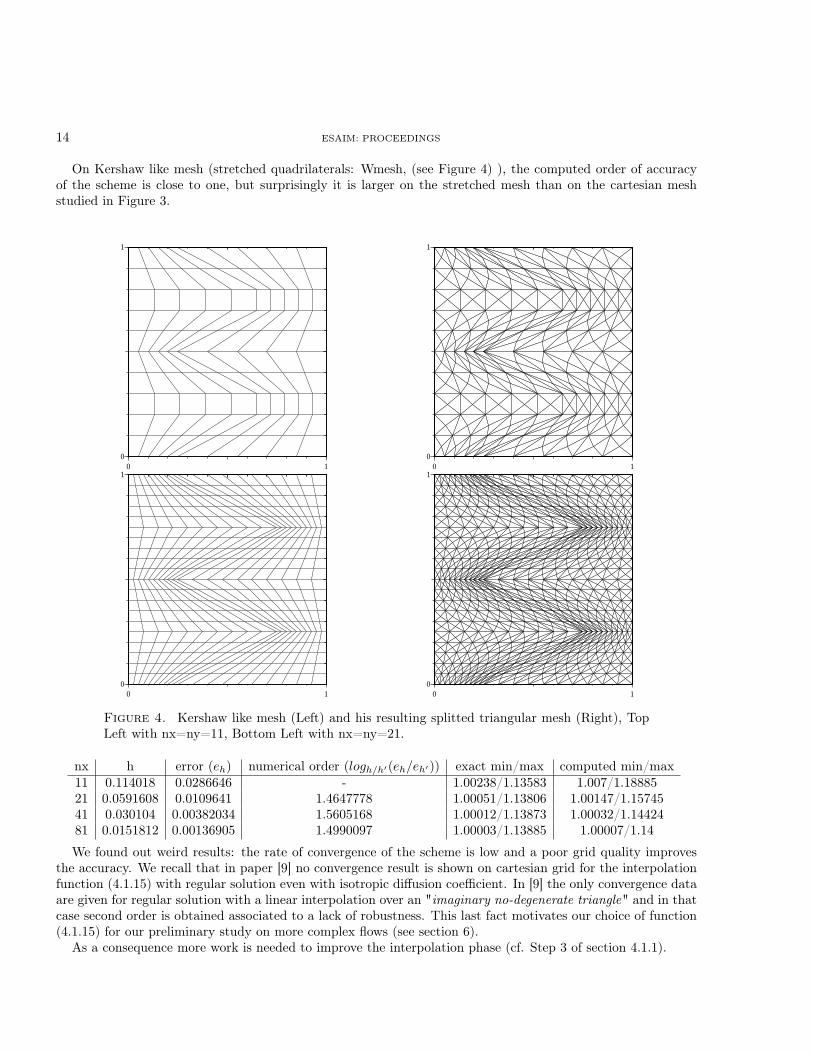
On Kershaw like mesh (stretched quadrilaterals: Wmesh, (see Figure 4) ), the computed order of accuracyof the scheme is close to one, but surprisingly it is larger on the stretched mesh than on the cartesian meshstudied in Figure 3.

0 10

1

0 10

1

0 10

1

0 10

1

Figure 4. Kershaw like mesh (Left) and his resulting splitted triangular mesh (Right), TopLeft with nx=ny=11, Bottom Left with nx=ny=21.

nx h error (eh) numerical order (logh/h′(eh/eh′)) exact min/max computed min/max11 0.114018 0.0286646 - 1.00238/1.13583 1.007/1.1888521 0.0591608 0.0109641 1.4647778 1.00051/1.13806 1.00147/1.1574541 0.030104 0.00382034 1.5605168 1.00012/1.13873 1.00032/1.1442481 0.0151812 0.00136905 1.4990097 1.00003/1.13885 1.00007/1.14

We found out weird results: the rate of convergence of the scheme is low and a poor grid quality improvesthe accuracy. We recall that in paper [9] no convergence result is shown on cartesian grid for the interpolationfunction (4.1.15) with regular solution even with isotropic diffusion coefficient. In [9] the only convergence dataare given for regular solution with a linear interpolation over an "imaginary no-degenerate triangle" and in thatcase second order is obtained associated to a lack of robustness. This last fact motivates our choice of function(4.1.15) for our preliminary study on more complex flows (see section 6).

As a consequence more work is needed to improve the interpolation phase (cf. Step 3 of section 4.1.1).

ESAIM: PROCEEDINGS 15

5.2. Test on discrete maximum/minimum principle

Now we want to study if the numerical scheme obeys the discrete maximum/minimum principle previouslyintroduce in (4.0.11). We deal with the following problem:

∂tc = ∆c in Ω = (0, 1) × (0, 1),

c0(x) = 1 − χ(x−0.5)2+(y−0.5)2<0.1 in Ω,

c = 1 on ∂Ω.

(5.2.1)

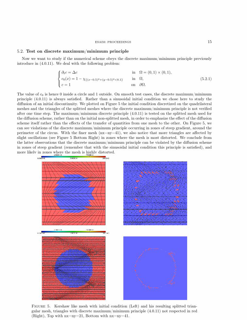
The value of c0 is hence 0 inside a circle and 1 outside. On smooth test cases, the discrete maximum/minimumprinciple (4.0.11) is always satisfied. Rather than a sinusoidal initial condition we chose here to study thediffusion of an initial discontinuity. We plotted on Figure 5 the initial condition discretized on the quadrilateralmeshes and the triangles of the splitted meshes where the discrete maximum/minimum principle is not verifiedafter one time step. The maximum/minimum discrete principle (4.0.11) is tested on the splitted mesh used forthe diffusion scheme, rather than on the initial non-splitted mesh, in order to emphasize the effect of the diffusionscheme itself rather than the effects of the transfer of quantities from one mesh to the other. On Figure 5, wecan see violations of the discrete maximum/minimum principle occurring in zones of steep gradient, around theperimeter of the circus. With the finer mesh (nx=ny=41), we also notice that more triangles are affected byslight oscillations (see Figure 5 Bottom Right) in zones where the mesh is most distorted. We conclude fromthe latter observations that the discrete maximum/minimum principle can be violated by the diffusion schemein zones of steep gradient (remember that with the sinusoidal initial condition this principle is satisfied), andmore likely in zones where the mesh is highly distorted.

Figure 5. Kershaw like mesh with initial condition (Left) and his resulting splitted trian-gular mesh, triangles with discrete maximum/minimum principle (4.0.11) not respected in red(Right), Top with nx=ny=21, Bottom with nx=ny=41.

16 ESAIM: PROCEEDINGS

6. Tests on Coupling with Hydrodynamic in ALE and Adaptation context

6.1. Passive diffusion of a scalar on moving mesh

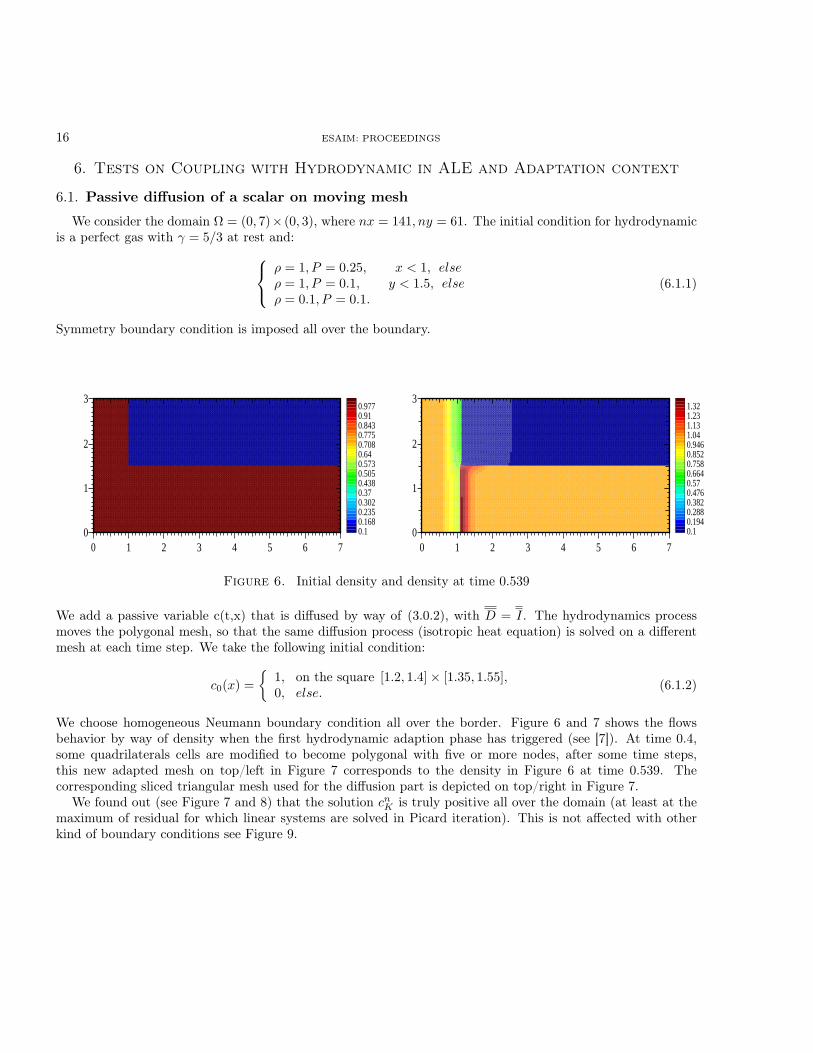
We consider the domain Ω = (0, 7)× (0, 3), where nx = 141, ny = 61. The initial condition for hydrodynamicis a perfect gas with γ = 5/3 at rest and:

ρ = 1, P = 0.25, x < 1, elseρ = 1, P = 0.1, y < 1.5, elseρ = 0.1, P = 0.1.

(6.1.1)

Symmetry boundary condition is imposed all over the boundary.

0 1 2 3 4 5 6 70

1

2

3

0.10.1680.2350.3020.370.4380.5050.5730.640.7080.7750.8430.910.977

0 1 2 3 4 5 6 70

1

2

3

0.10.1940.2880.3820.4760.570.6640.7580.8520.9461.041.131.231.32

Figure 6. Initial density and density at time 0.539

We add a passive variable c(t,x) that is diffused by way of (3.0.2), with D = I. The hydrodynamics processmoves the polygonal mesh, so that the same diffusion process (isotropic heat equation) is solved on a differentmesh at each time step. We take the following initial condition:

c0(x) =

1, on the square [1.2, 1.4] × [1.35, 1.55],0, else.

(6.1.2)

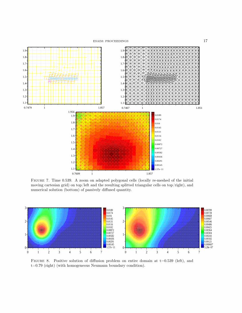
We choose homogeneous Neumann boundary condition all over the border. Figure 6 and 7 shows the flowsbehavior by way of density when the first hydrodynamic adaption phase has triggered (see [7]). At time 0.4,some quadrilaterals cells are modified to become polygonal with five or more nodes, after some time steps,this new adapted mesh on top/left in Figure 7 corresponds to the density in Figure 6 at time 0.539. Thecorresponding sliced triangular mesh used for the diffusion part is depicted on top/right in Figure 7.

We found out (see Figure 7 and 8) that the solution cnK is truly positive all over the domain (at least at the

maximum of residual for which linear systems are solved in Picard iteration). This is not affected with otherkind of boundary conditions see Figure 9.

ESAIM: PROCEEDINGS 17

0.7479 1 1.857

1.1

1.2

1.3

1.4

1.5

1.6

1.7

1.8

1.9

0.7467 1 1.851

1.1

1.2

1.3

1.4

1.5

1.6

1.7

1.8

1.9

0.7609 1 1.857

1.1

1.2

1.3

1.4

1.5

1.6

1.7

1.8

1.91.956

1.57e−11

0.00145

0.00291

0.00436

0.00582

0.00727

0.00872

0.0102

0.0116

0.0131

0.0145

0.016

0.0174

0.0189

Figure 7. Time 0.539. A zoom on adapted polygonal cells (locally re-meshed of the initialmoving cartesian grid) on top/left and the resulting splitted triangular cells on top/right), andnumerical solution (bottom) of passively diffused quantity.

0 1 2 3 4 5 6 70

1

2

3

1.57e−110.001450.002910.004360.005820.007270.008720.01020.01160.01310.01450.0160.01740.0189

0 1 2 3 4 5 6 70

1

2

3

5.28e−070.0006070.001210.001820.002430.003040.003640.004250.004860.005460.006070.006680.007280.00789

Figure 8. Positive solution of diffusion problem on entire domain at t=0.539 (left), andt=0.79 (right) (with homogeneous Neumann boundary condition).

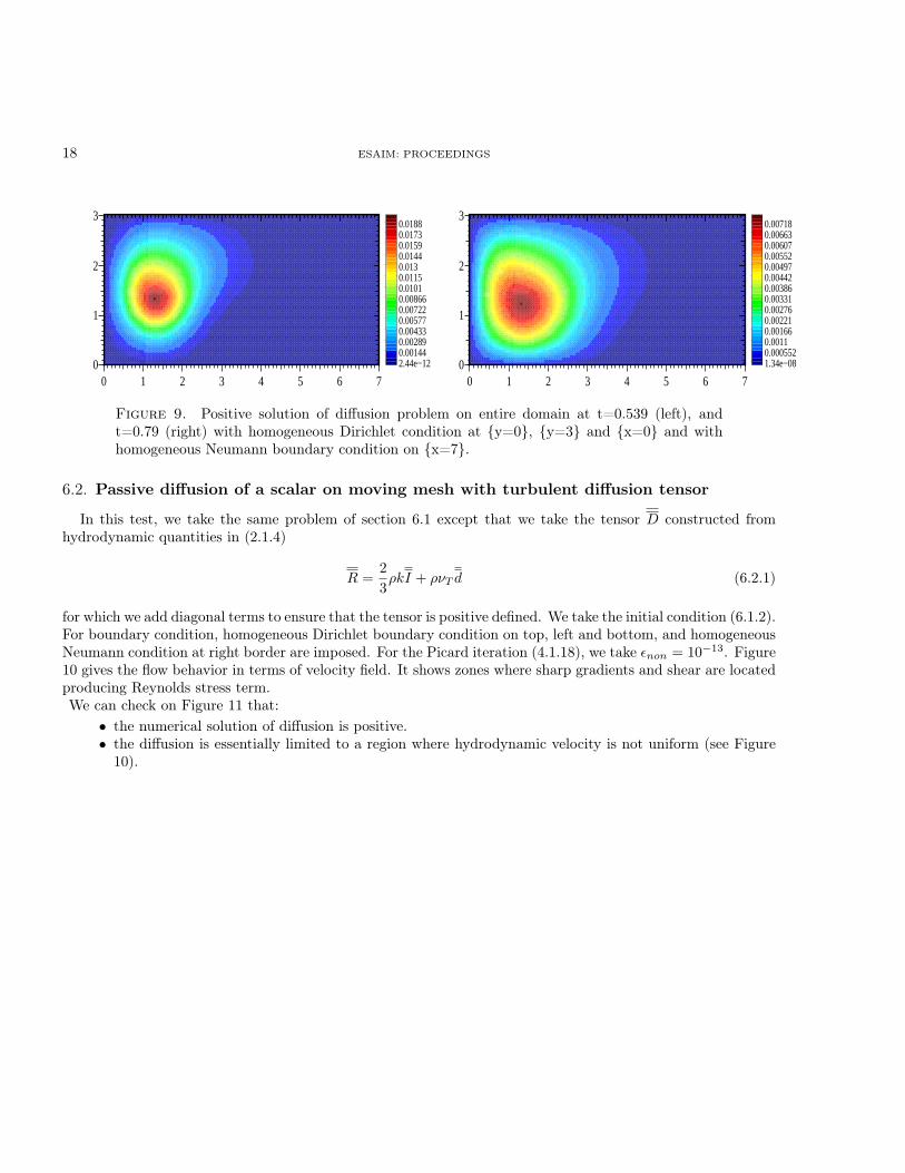
18 ESAIM: PROCEEDINGS

0 1 2 3 4 5 6 70

1

2

3

2.44e−120.001440.002890.004330.005770.007220.008660.01010.01150.0130.01440.01590.01730.0188

0 1 2 3 4 5 6 70

1

2

3

1.34e−080.0005520.00110.001660.002210.002760.003310.003860.004420.004970.005520.006070.006630.00718

Figure 9. Positive solution of diffusion problem on entire domain at t=0.539 (left), andt=0.79 (right) with homogeneous Dirichlet condition at y=0, y=3 and x=0 and withhomogeneous Neumann boundary condition on x=7.

6.2. Passive diffusion of a scalar on moving mesh with turbulent diffusion tensor

In this test, we take the same problem of section 6.1 except that we take the tensor D constructed fromhydrodynamic quantities in (2.1.4)

R =2

3ρkI + ρνT d (6.2.1)

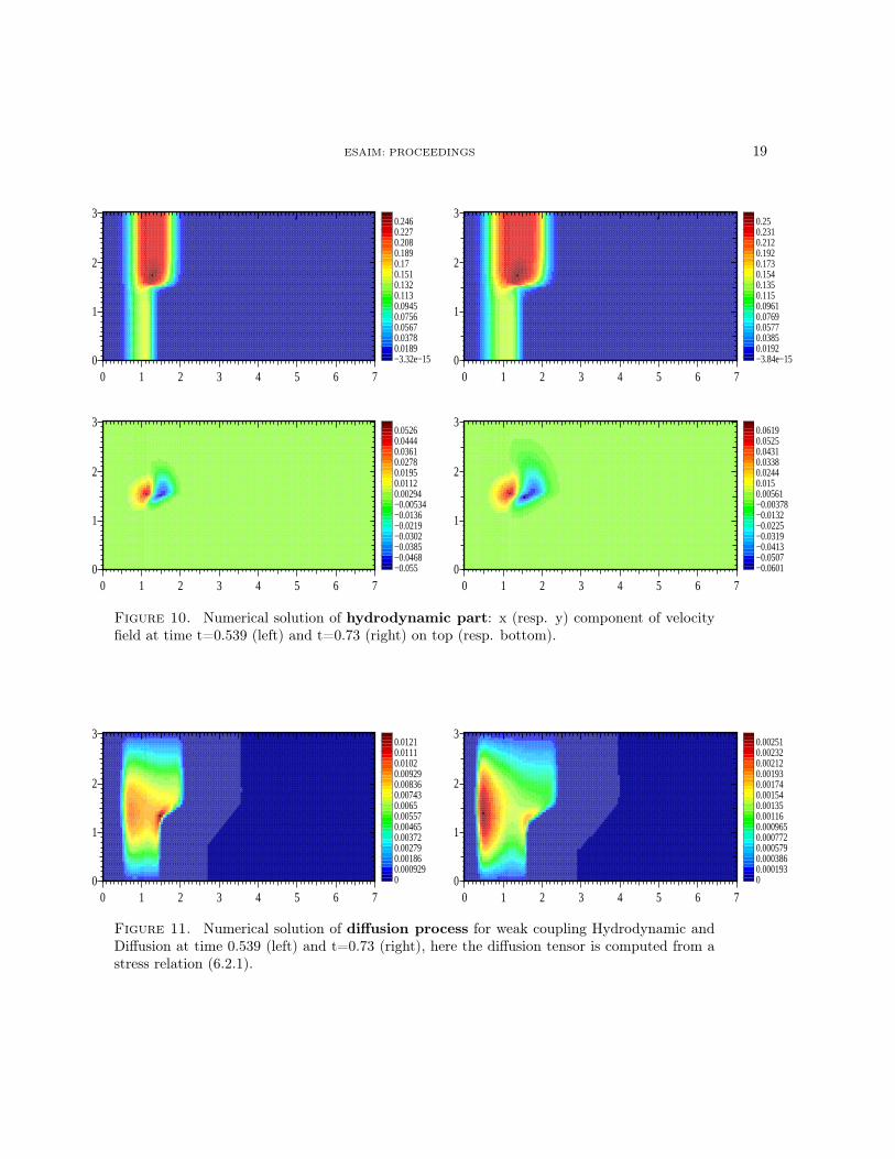
for which we add diagonal terms to ensure that the tensor is positive defined. We take the initial condition (6.1.2).For boundary condition, homogeneous Dirichlet boundary condition on top, left and bottom, and homogeneousNeumann condition at right border are imposed. For the Picard iteration (4.1.18), we take ǫnon = 10−13. Figure10 gives the flow behavior in terms of velocity field. It shows zones where sharp gradients and shear are locatedproducing Reynolds stress term.We can check on Figure 11 that:

• the numerical solution of diffusion is positive.• the diffusion is essentially limited to a region where hydrodynamic velocity is not uniform (see Figure

10).

ESAIM: PROCEEDINGS 19

0 1 2 3 4 5 6 70

1

2

3

−3.32e−150.01890.03780.05670.07560.09450.1130.1320.1510.170.1890.2080.2270.246

0 1 2 3 4 5 6 70

1

2

3

−3.84e−150.01920.03850.05770.07690.09610.1150.1350.1540.1730.1920.2120.2310.25

0 1 2 3 4 5 6 70

1

2

3

−0.055−0.0468−0.0385−0.0302−0.0219−0.0136−0.005340.002940.01120.01950.02780.03610.04440.0526

0 1 2 3 4 5 6 70

1

2

3

−0.0601−0.0507−0.0413−0.0319−0.0225−0.0132−0.003780.005610.0150.02440.03380.04310.05250.0619

Figure 10. Numerical solution of hydrodynamic part: x (resp. y) component of velocityfield at time t=0.539 (left) and t=0.73 (right) on top (resp. bottom).

0 1 2 3 4 5 6 70

1

2

3

00.0009290.001860.002790.003720.004650.005570.00650.007430.008360.009290.01020.01110.0121

0 1 2 3 4 5 6 70

1

2

3

00.0001930.0003860.0005790.0007720.0009650.001160.001350.001540.001740.001930.002120.002320.00251

Figure 11. Numerical solution of diffusion process for weak coupling Hydrodynamic andDiffusion at time 0.539 (left) and t=0.73 (right), here the diffusion tensor is computed from astress relation (6.2.1).

20 ESAIM: PROCEEDINGS

7. Conclusion and extensions

In this paper, we present a way to treat a weak coupling between hydrodynamics and diffusion problem onarbitrary polygonal mesh. The diffusion component part of the solution is computed on the moving mesh givenby the hydrodynamics and the diffusion tensor is computed by a relation depending on the gradient of velocityof the flows to modelize a turbulent behavior.Future works will include a way to obtain a diffusion scheme satisfying a good convergence behavior (seenumerical tests in section 5) and then the Discrete Maximum Principle on arbitrary unstructured triangularmesh. With our alternative based on the partitioning of polygons in triangles, we could deal with star shapedpolygonal cells (see also for instance the recent paper [15]). We will then come back to a strong coupling betweendiffused concentration and hydrodynamics.

References

[1] G. Barles. Solutions de viscosité des équations de Hamilton-Jacobi. Springer, 1995.

[2] J.D. Benamou and P. Hoch. Go++ : A modular lagrangian/eulerian software for hamilton jacobi equations of geometric opticstype. M2AN, 36(5):883–905, 2002.

[3] A. Chambolle and B.J. Lucier. A maximum principle for order-preserving mappings. C.R.A.S, 326:823–827, 1998.

[4] P.G. Ciarlet and P.A. Raviart. Maximum principle and uniform convergence for the finite element method. Comput. Methods

Appl. Mech. Engrg., 2:17–31, 1973.[5] P. Frey and P.L. George. Mesh Generation Application to Finite Elements. Hermes Science Publications, 2000.[6] A. Friedman. Partial Differential Equations of the Parabolic Type. Prentice-Hall, 1964.[7] P. Hoch, S. Marchal, Y. Vasilenko, and A.A. Feiz. Non conformal adaptation and mesh smoothing for compressible lagrangian

fluid dynamics. ESAIM, 24:111–129, 2008.[8] D. Kershaw. Differencing of the diffusion equation in lagrangian hydrodynamic codes. Journal Of Comput. Physics, (39):375–

395, 1981.[9] K. Lipnikov, S. Shashkov, D. Svyatskiy, and Yu. Vassilevski. Monotone finite volume schemes for diffusion equations on

unstructured triangular and shape-regular polygonal meshes. Journal Of Comput. Physics, (227):492–512, 2007.

[10] G.J. Pert. Physical constraints in numerical calculations of diffusion. Journal Of Comput. Physics, (42):20–52, 1981.[11] C. Le Potier. Schéma volumes finis monotone pour des opérateurs de diffusion fortement anisotropes sur des maillages de

triangles non-structurés. C.R. Acad. Sci., (Ser I 341):787–792, 2005.[12] Alfio Quarteroni, Riccardo Sacco, and Fausto Saleri. Méthodes Numériques: Algorithmes, Analyse Et Applications. Springer

Verlag, 2007.[13] D. Shepard. A two-dimensional interpolation function for irregularly spaced data. In 23d ACM National Conference, pages

517–524, NY, 1968.[14] O. Soulard and D. Souffland. A second order turbulent closure for modeling counter-gradient transport in variable density

turbulent flows. ICHMT digital library, (1):369–372, 2006.[15] Guangwei Yuan and Zhiqiang Sheng. Monotone finite volume schemes for diffusion equations on polygonal meshes. J. Comput.

Phys., 227(12):6288–6312, 2008.