Root Locus Analysis of a Retarded Quasipolynomial

Root Locus Analysis of a Retarded Quasipolynomial

LIBOR PEKAŘ Department of Automation and Control, Faculty of Applied Informatics

Tomas Bata University in Zlín nám. T. G. Masaryka 5555, 76001 Zlín

CZECH REPUBLIC [email protected]

Abstract: - Time delay systems (TDS), called hereditary or anisochronic as well, can be frequently found in many engineering problems and they constitute a widespread family of industrial plants. Modelling, identification, stability analysis, stabilization, control, etc. of TDS are challenging and fascinating tasks in modern systems and control theory as well as in academic and industrial applications. One of their possible linear representations in the form of the Laplace transform yields the transfer function expressed as a fraction of quasipolynomials, instead of polynomials, with delay (exponential) terms in denominators. In this contribution, detailed root location analysis of a characteristic retarded quasipolynomial of degree one is presented, which gives rise to the spectrum of a retarded TDS. The presented analysis represents also a powerful tool for controller tuning in pole-placement control algorithms for delayed systems. A simulation example clarifies the results obtained vie proven propositions, lemmas and theorems. Key-Words: - Time delay systems, root locus, stability analysis, retarded quasipolynomials 1 Introduction Delay as a generic part of many processes is a phenomenon which unambiguously deteriorates the quality of a feedback control performance, such as stability, periodicity, etc. Modern control theory has been dealing with this problem for longer than five decades, since the era of the Smith predictor [1]. Linear time-invariant time delay systems (LTI-TDS) in technological and other processes are sometimes assumed to contain delay elements in input-output relations only, which results in shifted arguments on the right-hand side of differential equations. All the system dynamics is hence modelled by point accumulations in the form of a set of ordinary differential equations (ODEs). The Laplace transform thus yields a transfer function expressed by a serial combination of a delay-free rational term and a delay exponential element. However, this conception is somewhat restrictive in effort to express the real plant dynamics since inner feedbacks can often be of time-distributed or delayed nature.

LTI-TDS in its modern meaning as anisochronic or hereditary models, in the contrary, offer a more universal dynamics description applying both integrators and delay elements on the left-hand side of a differential equation, either in a lumped or distributed form, yielding functional differential equations (FDEs). Using some techniques [2], [3]

one can reduce possible integrals to a combination of shifted-argument output or state variables elements (without loosing information), which finally gives a transfer function as a ratio of so called quasipolynomials [4] with an infinite number of poles. For LTI-TDS without distributed delays in an input or in an output relation, the denominator quasipolynomial decides about its asymptotic (exponential) stability.

Already Volterra [5] (according to [6]) formulated differential equations incorporating the past states when he was studying predator-pray models. The theory of these models was then rediscovered and developed e.g. in [6-10], to name but a few. Some possibilities and advantages of this class of models and controllers for modeling and process control are discussed in [11].

These models are applied in processes with energy or mass transportation phenomena, e.g. in chemical processes [12], in heat exchange networks [13], [14], in internal combustion engines with catalytic converter [15], in models of mass flow in sugar factory [16], in metallurgic processes [17], etc.

A huge number of books, conference and journal papers were dedicated to (exponential, asymptotic) stability analysis of systems with delay elements on the left-hand side of FDEs (see e.g. [8], [9], [18]-[26]); nevertheless, general approaches lacking detailed root locus analysis of a particular

WSEAS TRANSACTIONS on SYSTEMS and CONTROL Libor Pekar

ISSN: 1991-8763 79 Issue 3, Volume 6, March 2011

denominator quasipolynomial prevail. This contribution, contrariwise, offers a deep roots location analysis of a simple quasipolynomial which, as a model transfer function denominator, is convenient to represent the dynamics of many hereditary as well as delay-free high order systems as proven e.g. in [27]-[28]. Moreover, we present stability properties depended on a real non-delay parameter instead that on a delay value, as usual in the literature. The information about a LTI-TDS poles location can serve engineers to decide quickly about the position of a dominant pole (or a pair of poles) location or to place closed-loop poles when the studied characteristic quasipolynomial.

The paper is organized as follows: the general description of LTI-TDS models and systems and that of quasipolynomials is presented in Section 2. TDS and quasipolynomial stability properties are introduced in Section 3. The main part of the contribution is presented in Section 4 where roots location properties of a simple quasipolynomial are derived. Finally, Section 5 contains a short explicative example demonstrating basic results.

2 LTI-TDS Model Anisochronic, hereditary or TDS linear time-invariant models in general can be described by state and output FDEs in the form

( ) ( )

( ) ( )

( ) ( )

( ) ( ) ( ) ( )

( ) ( )tt

dtdt

tt

tt

tt

tt

LL

N

iii

N

iii

N

i

ii

B

A

H

Cxy

uBxA

uBuB

xAxA

xHx

=

−+−+

−++

−++

−=

∫∫

∑

∑

∑

=

=

=

00

10

10

1 dd

dd

ττττττ

η

η

η

(1)

where Ñ∈x n is a vector of state variables, ∈u Ñm stands for a vector of inputs, Ñ∈y l represents a vector of outputs, Ai, A(τ), BBi, B(τ), C, Hi are real matrices of compatible dimensions, Li ≤≤η0 stand for lumped delays and convolution integrals express distributed delays. If for any i = 1,2,...N

0H ≠i

H, model (1) is called neutral; on the other hand, if for every i = 1,2,...N0H =i H, so-called retarded model is obtained. It should be noted that

the state of model (1) is given not only by a vector of state variables in the current time, but also by a segment of the last model history of state and input variables ( ) ( ) [ 0,,, Ltt − ]∈++ τττ ux (2)

Model (1) can also be expressed in more consistent functional form using Riemann-Stieltjes integrals so that both lumped and distributed delays are under one convolution

( ) ( )

( ) ( ) ( ) ( )

( ) ( )tt

tt

tt

tt

LL

N

i

ii

H

Cxy

uBxA

xHx

=

−+−+

−=

∫∫

∑=

00

1

dd

dd

dd

ττττ

η

(3)

see details in [2]. Integrals in (1) can be rewritten into sums using

the Laplace transform, which is suitable for model implementation in computers and for simulations, using either exact transformation [2], [3] or via a standard numerical approximation methods. However, the latter approaches can destabilize even a stable model in some cases; see e.g. [19] and references herein. The transform correspondence is the following

(4) ( ) ( ) ( ) ( ) ( )

( ) ( ) ( ) ( ) ( )∫∫

∫∫

−=⎭⎬⎫

⎩⎨⎧

−

−=⎭⎬⎫

⎩⎨⎧

−

LL

LL

sst

sst

00

00

dexpd

dexpd

ττττττ

ττττττ

BUuB

AXxA

L

L

where {}⋅L denotes the Laplace transform operation. Subsequent utilization of the reverse Laplace transform yields the state equation in the form

( ) ( ) ( ) ( )

( ) ( )

( ) ( ) ( ) T

1

10

1

10

1

dd

~~

~~d

d~d

d

⎥⎦⎤

⎢⎣⎡=

−++

−++−

=

∑

∑∑+

=

+

==

tttt

tt

ttt

ttt

B

AH

N

iii

N

iii

N

i

ii

xxz

zBzB

zAzAzHz

η

ηη

(5)

where L

BA NN == ++ 11 ηη . Notice that authors’ interest is in retarded models

and systems due to their higher practical usability [14]-[17]; moreover, retarded systems have also some grateful features, for instance, the number of



poles in the right-half plane is the finite [5]. Considering, hence, a model of retarded type and zero initial conditions, the following input-output description and the transfer matrix using the Laplace transform from (5) is obtained

( ) ( ) ( )

( )

( )

( ) ( )ss

ss

ss

sss

B

A

A

N

iii

N

iii

N

iii

UBB

AAI

AAIC

UGY

⎥⎦⎤

⎢⎣⎡ −+

⎥⎦⎤

⎢⎣⎡ −−−

⎥⎦⎤

⎢⎣⎡ −−−

=

=

∑

∑

∑

+

=

+

=

+

=

1

10

1

10

1

10

exp~~

exp~~det

exp~~adj

η

η

η (6)

The main advantage of the anisochronic system

description in the form of the transfer function rests in its practical usability when system analysis and control design.

All transfer functions in have identical denominator in the form

( )sG

( ) ( )

( )∑∑

∑

−

= =

+

=

−+=

⎥⎦⎤

⎢⎣⎡ −−−=

1

0 1

1

10

exp

exp~~det

n

i

h

jij

iij

n

N

iii

i

A

ssms

sssm

η

ηAAI (7)

where

⎟⎟⎠

⎞⎜⎜⎝

⎛−

−+≤

ininN

h Ai (8)

which arises from the calculation of all permutations in the determinant; since, the upper bound of equals the number of all combinations with repetitions of N

ih

A+1 elements choose (n-i). Thenceforward, a simple-input simple-output

system is considered, which gives rise to the transfer function (6) in the form of a ratio of quasipolynomials instead of transfer function matrix.

3 Asymptotic Stability Formula (7) expresses the characteristic quasipolynomial of retarded type of system (1). If there are no distributed delays in the model or they are approximated by a numerical method, the quasipolynomial determines the system poles, σi, by solution of . However, in the case of distributed delays, the quasipolynomial zeros do not agree with the systems spectrum, since some

transfer function denominator roots are those of the numerator, and thus they do not affect the system dynamics. Due to the transcendental character of model (1) caused by exponential terms, the number of poles is infinite in general and anisochronic models are regarded as infinite-dimensional. The role of zeros is the same as for delay-free systems and the number of zeros depends on the structure of numerators in (6).

( ) 0=sm

The system asymptotic stability is formulated in the same way as for delay-free systems; hence, it is determined by system poles. LTI-TDS is stable iff

( ) ( ){ } 00:Resup: <== ii m σσσ (9)

i.e. all system poles are located in the open left half complex plane, see, e.g. [15], [16].

Both types of systems, retarded and neutral ones, embody diverse spectral properties w.r.t. poles locations and their changes depended on changes of quasipolynomials parameters. Whereas retarded systems always own finite number of unstable poles, unstable neutral systems have infinite number of these poles which constitute vertically bounded strips [5], [25]. Another important feature is that poles locations of the retarded type is continuously depended on delays iη , while small changes in delays for neutral systems can cause abrupt changes in the spectrum. Hence, condition (9) is deficient in order to express the “whole” asymptotic stability of neutral LTI-TDS which bought the concept of so called strong stability [23].

Besides analytic tools for searching spectra of delayed systems via the knowledge of characteristic quasipolynomials, powerful numeric approaches were also investigated. The solved task can be reduced to computing roots of a general analytic function. Weyl’s algorithm [22] and Quasipolynomial Mapping Based Rootfinder (QPMR) [23, 24] can be named as examples of such algorithms.

It is hence possible to investigate the LTI-TDS asymptotic stability via root location analysis of the characteristic quasipolynomial, in the case of lumped delays.

4 Retarded Quasipolynomial Root Locus The main goal of this contribution is to study spectral properties of a simple retarded quasipolynomial given by



( ) ( )sqssm τ−+= exp (10) where ∈s Â, Ñ, ∈q ∈τ Ñ+, with respect to the non-delay real parameter q while τ is fixed. It was demonstrated [27], [28] that models of dynamics described by this quasipolynomial as a transfer function denominator, can be successfully used for the description of a real plant dynamics of conventional (delay-free) high order systems. Stability properties of quasipolynomial (10) have been already studied in [9]. In [28] the roots location of (10) using QPMR was investigated; however, a deeper analysis was not made.

First, we investigate the case when the roots cross the imaginary axis. Lemma 1. Quasipolynomial (10) has a root, a real or a complex conjugate pair, on the imaginary axis (i.e. on the asymptotic stability border) iff

,0=q ( ) ( ) ,...2,1,0,2

121 =+−= kkq k

τπ (11)

Moreover it holds that q±=ω (12) where ω is the imaginary part of the root. ■ Proof. For the necessity, consider a real root on the imaginary axis, σ = 0, first. Thus, it must hold thatt

(13) ( )

0010

0exp=⇒

⎭⎬⎫

=+=−+

qqq τσσ

Second, if complex conjugate roots with non-zero imaginary parts are taken into account, 0,j >±= ωωασ , condition ( ) 0=σm can also be expressed as

( ) ( )( ) ( ) 0sinexp

0cosexp=−−=−+

τωταωτωταα

qq

(14)

Taking a pair of roots purely on the imaginary axis, 0,j >±= ωωσ , conditions (14) are reduced into

( )( ) ωτωτω

==

sin0cos

qq

(15)

The former condition gives

0=q or ,...2,1,0,2

=+= kkππτω (16)

Whereas condition 0=q , inserting into the latter relation in (15), gives a real root only, the latter equality in (16) yields

( )⎩⎨⎧

=−=

==+= ,...5,3,1,1

,...4,2,0,1sin

,..2,1,0,2 k

kkkππτω

τω (17)

hence from (15) we have

⎪⎩

⎪⎨

⎧

=+

−=−

=+

==

,...5,3,1,22

,...4,2,0,22

kk

kk

q

τππω

τππω

(18)

which agrees with the lemma statement (=>). Sufficiency (<=) can be easily proved in a similar way by inserting q into (14). ü Lemma 1 gives no information about other roots positions so that we can not decide about the rest of the quasipolynomial spectrum. The following lemmas clarify positions of other roots of (10) when (11) holds. To prove the lemmas, a significant theorem formulated e.g. in [29] has to be presented. Theorem 1 (Root continuity). Let and the sequence

( )sf( ){ } 1≥nn sf be analytic function on an

(open) domain Ã Â. Suppose that ⊆ ( ){ } 1≥nn sf converges uniformly to on the disc ( )sf

{ }⊆≤−= rssD 0: σ Ã for some r > 0 and that on this disc 0σ is the only zero of ( )sf with multiplicity k. Then there exists a natural number N such that Nn ≥∀ , ( )sf has exactly k zeros 1,nσ , ...,

kn,σ in D and { kjjnn ,...,1,lim 0, ∈∀=∞→ }σσ . ■ For a proof of Theorem 1, see [29]. Theorem 1 implies another important fact that retarded quasipolynomial has roots continuous w.r.t. changes of q. That is, a limit sequence of quasipolynomials (with infinitesimal changes of q) results in a corresponding limit sequence of roots of

( )sm

( )sm . Lemma 2. For q = 0, there is no root in the open right half complex plane. ■ Proof. We will show a contradiction. Take q = 0 and suppose that there it exists a positive (unstable) real root of (10), 0>=ασ . Videlicet, ( ) 00exp0 =⇒=−+ αταα (19)



Similarly, assume a complex conjugate root with a positive real part, i.e. 0,j >±= αωασ . Equations (14) give rise to

(20) ( ) ( )( ) ( ) 0

0sinexp00cosexp0

==⇒⎭⎬⎫

=−−=−+

ωατωταωτωταα

Thus we have a contradiction again. ü Note that further (in Proposition 5) we will show that there are infinity many roots with a real part

−∞=α for q = 0. Lemma 3 (Roots shift tendency). Define two sets

of q as 21,ΣΣ

( )⎭⎬⎫

⎩⎨⎧ =+==Σ ,..2,1,0,

214::1 kkqq

τπ

( )

⎪⎭

⎪⎬⎫

⎪⎩

⎪⎨⎧

=

+−===Σ

,..2,1,0

,2

34or 0::2

k

kqqqτπ

(21)

and two corresponding spectra of ( )sm

Â⎩⎨⎧ ∈=Θ σ:1 ( )

⎭⎬⎫=

Σ∈0:

1qm σ

Â⎩⎨⎧ ∈=Θ σ:2 ( )

⎭⎬⎫=

Σ∈0:

2qm σ (22)

Then the following statements hold: 1) If where for arbitrarily small , then the spectrum of have one root (real or complex conjugate pair) in the open right half complex plane more in comparison with

.

Δ+= rq 1Σ∈r0>Δ ( )sm

1Θ 2) If where Δ+= rq 2Σ∈r for arbitrarily small

, then the spectrum of have one root (real or complex conjugate pair) in the open left half complex plane more in comparison with . ■

0>Δ ( )sm

2Θ Proof. Lemma 1 certifies that with ( )sm 1Σ∈q or has a root 2Σ∈q σ (real or a conjugate pair of roots) located exactly on the imaginary axis where qjj ±=±= ωσ . Theorem 1 says that an arbitrary small change of q results in small shifting in roots locations. Hence, if or 1Σ∈q 2Σ∈q is increased byΔ , a root on the imaginary axis moves to a new position close to the imaginary axis. The question is whether the root moves to the right

(unstable) half complex plane or to the left (stable) one. To solve the problem, we calculate the sensitivity function ( )qsS , defined as

( )( )

( )( )

( )sqs

sqsm

qqsm

qsqsS

τττ−−

−−=

∂∂∂

∂

−=∂∂

=exp1

exp,

,

, (23)

at a point 21,ΣΣ∈q , qs j±= . The sensitivity function (23) determines the tendency (direction) of roots of to shift in the complex plane while a small changing of . The aim is to decide whether the root on the imaginary axis moves to the right or to the left, i.e. it is sufficient to take the real part of only, which for

( )smq

( qsS , )ωα j±=s reads

( )

( ) ( )[ ] ( )( )( ) ( ) ( ) τωταττατ

ατωταττqq

qqsS

cosexp22exp1expcosexp

,Re

2 −−−+−−−

=(24)

Hence 1) for 1Σ∈q , qs j±=

( )

( )

( )

,...2,1,0

0

2141

214

,Re 2j1

=

>

⎥⎦⎤

⎢⎣⎡ ++

+=

±=Σ∈

k

k

kqsS

qsq

π

π

(25)

2) for }0{\2Σ∈q , qs j±=

( )

( )

( )

,...2,1,0

0

2341

234

,Re 2j}0{\2

=

<

⎥⎦⎤

⎢⎣⎡ ++

+−=

±=Σ∈

k

k

kqsS

qsq

π

π

(26)

3) for q = 0, s = 0 ( ) 1,Re

00 −=

==

sqqsS (27)

Expression (25) implies that for , the root on imaginary axis tends to shift to the right half complex plane if q is increased by Δ. Contrariwise

1Σ∈q



from (26) and (27), whenever is increased by Δ, the root moves to the stable, left half complex plane. ü

2Σ∈q

Notice that is non-positive, thus we can generalize the finding such that if

2Σ∈qq (where

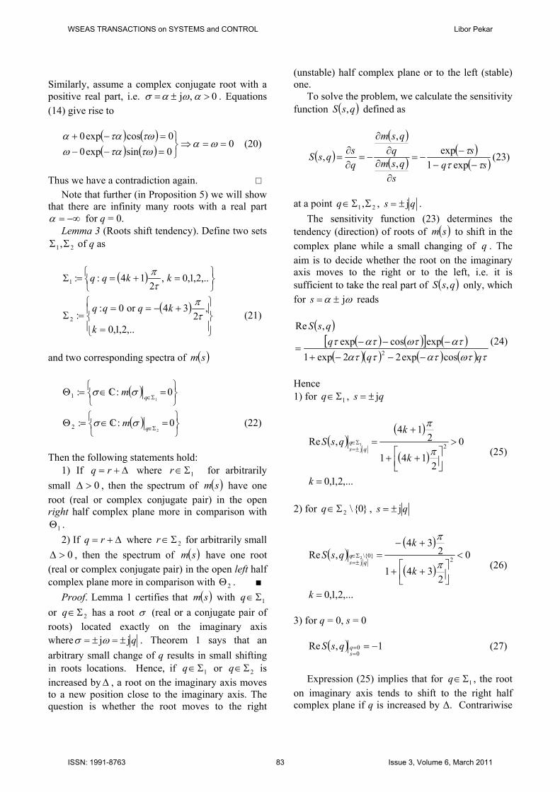
) is increased, the root on the imaginary axis moves to the right (unstable) half complex plane. Moreover, whereas the shifting in the imaginary axis is non-zero for , the zero root shifts only in the real axis (not analyzed here – this can be done by calculating imaginary parts of the sensitivity function). The situation is illustrated in Fig. 1.

21,ΣΣ∈q

0≠q

Theorem 2. (Quasipolynomial stability). Quasipolynomial (10) has all roots in the open left half complex plane iff

⎟⎠⎞

⎜⎝⎛∈

τπ2

,0q (28)

■ Proof. (Necessity) Consider first and apply Lemma 2 and Lemma 3. According to Lemma 2, there is no unstable root for and Lemma 3 declares that the root shifts to the right half complex plane for

0<q

0=q0=qΔ−=q (recall that Δ is

arbitrarily small positive real number). Hence, 0<q results in an unstable quasipolynomial m(s).

Second, let τπ2

>q . Lemma 2 declares that the

root on the imaginary axis for τπ2

=q , i.e.

τπσ2

j2,1 ±= , tends to shift to the right for

Δ+=τπ2

q , see Fig. 1. We have a contradiction

again. The result of Theorem 2 has already been presented in [9]. Proposition 1. There exists a double real root

τσ 1

−= in the spectrum of m(s) iff ( )1exp1

τ=q . ■

Proof. (Necessity) Take τ

σ 1−= and set

( ) 0=σm . This equation gives ( )1exp1

τ=q .

(Sufficiency) Taking ( )1exp1

τ=q it is satisfied

( ) 01 =− −τm .

Fig. 1. Root shifting tendency for 21,ΣΣ∈q on the imaginary axis

It must be proved that τ

σ 1−= is a double root.

Calculate

( ) ( ) ( )

( ) ( ) ( )sqs

smsm

sqssmsm

ττ

ττ

−==′′

−−==′

expd

d

exp1d

d

22

2 (30)

One can easily prove that ( ) 01 =′ −=τs

sm and

( ) 01 ≠′′ −=τssm which verifies that the real root is

double. ü Let us now derive and display a figure that clarifies the further statements. By omitting q in (15) the inevitable relation between real and imaginary parts of the roots is ( )τωωα cot=− (31) Denote a real part of a root as

∈−= 00 , k

kτ

α Ñ (32)

which is a multiple of the “critical” root from Proposition 1. Hence

( ) ( )τωτω tan1

0

=k

(33)



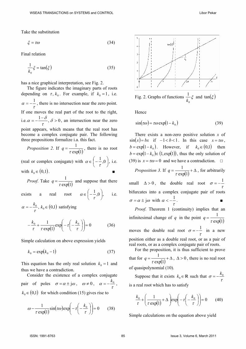
Take the substitution τωξ = (34) Final relation

( )ξξ tan1

0

=k

(35)

has a nice graphical interpretation, see Fig. 2. The figure indicates the imaginary parts of roots depending on 0, kτ . For example, if 10 =k , i.e.

τα 1

−= , there is no intersection near the zero point.

If one moves the real part of the root to the right,

i.e. 0,1>

−−= δ

τδα , an intersection near the zero

point appears, which means that the real root has become a complex conjugate pair. The following three propositions formalize i.a. this fact.

Proposition 2. If ( )1exp1

τ=q , there is no root

(real or complex conjugate) with ⎟⎠⎞

⎜⎝⎛−∈ 0,1

τα , i.e.

with . ■ ( )1,00 ∈k

Proof. Take ( )1exp1

τ=q and suppose that there

exists a real root ⎟⎠⎞

⎜⎝⎛−∈ 0,1

τα , i.e.

( )1,0, 00 ∈−= kkτ

α satisfying

( ) 0exp1exp

1 00 =⎟⎟⎠

⎞⎜⎜⎝

⎛⎟⎠⎞

⎜⎝⎛−−+−

ττ

ττkk

(36)

Simple calculation on above expression yields (37) ( 1exp 00 −= kk ) This equation has the only real solution 10 =k and thus we have a contradiction. Consider the existence of a complex conjugate

pair of poles ωασ j±= , 0≠ω , τ

α 0k−= ,

for which condition (15) gives rise to ( 1,00 ∈k )

( ) ( ) 0expsin1exp

1 0 =⎟⎟⎠

⎞⎜⎜⎝

⎛⎟⎠⎞

⎜⎝⎛−−−

τττω

τω

k (38)

Fig. 2. Graphs of functions ξ

0

1k

and ( )ξtan

Hence ( ) ( )01expsin k−=τωτω (39) There exists a non-zero positive solution x of

( ) bxx =sin if 11 <<− b . In this case τω=x , ( )01exp kb −= . However, if ( )1,00 ∈k then ( ) ( )( )1exp,11exp 0 ∈−= kb , thus the only solution of

(39) is 0==τωx and we have a contradiction. ü

Proposition 3. If ( ) Δ+=1exp

1τ

q , for arbitrarily

small 0>Δ , the double real root τ

σ 1−=

bifurcates into a complex conjugate pair of roots

ωασ j±= with τ

α 1−< . ■

Proof. Theorem 1 (continuity) implies that an

infinitesimal change of in the point q ( )1exp1

τ=q

moves the double real root τ

σ 1−= in a new

position either as a double real root, or as a pair of real roots, or as a complex conjugate pair of roots. For the proposition, it is thus sufficient to prove

that for ( ) Δ+=1exp

1τ

q , , there is no real root

of quasipolynomial (10).

0>Δ

Suppose that it exists Ñ such that ∈0kτ

σ 0k−=

is a real root which has to satisfy

( ) 0exp1exp

1 00 =⎟⎟⎠

⎞⎜⎜⎝

⎛⎟⎠⎞

⎜⎝⎛−−⎟⎟

⎠

⎞⎜⎜⎝

⎛Δ++

ττ

ττkk

(40)

Simple calculations on the equation above yield



( )( ) ( 1exp1exp1 00 )−Δ+= kk τ (41) Since ( )( 11exp1 >Δ+ )τ one can easily prove that there is no real as a solution (13) and thus there is no real root.

0k

Now we use Figure 2 as a solution map of (31) and (33) which clearly indicates that there is a complex conjugate root with ω near zero,

then , i.e. 10 0 << k 01<<− α

τ. ü

Proposition 4. If ( ) Δ−=1exp

1τ

q , for arbitrarily

small , then the double real root 0>Δτ

σ 1−=

becomes two (different) real roots 21, σσ with

τσ 1

1 −< and τ

σ 12 −> , respectively. ■

Proof. W.r.t. Theorem 1, it ought to be shown

that for ( ) Δ−=1exp

1τ

q , 0>Δ , quasipolynomial

(10) has two different real roots. In other words,

δτ

σ +=−= 1, 0101

1 kk , 0>δ and τ

σ 022

k−= ,

δ−=102k , 0>δ respectively, must satisfy

( )

( ) 0exp1exp

1

0exp1exp

1

0202

0101

=⎟⎟⎠

⎞⎜⎜⎝

⎛⎟⎠⎞

⎜⎝⎛−−⎟⎟

⎠

⎞⎜⎜⎝

⎛Δ−+

=⎟⎟⎠

⎞⎜⎜⎝

⎛⎟⎠⎞

⎜⎝⎛−−⎟⎟

⎠

⎞⎜⎜⎝

⎛Δ−+

ττ

ττ

ττ

ττ

kk

kk

(42)

The latter gives

( )( )1exp

1exp+−−

=Δδτδδ (43)

whereas the former yields

( )( )1exp

1exp+−−+−

=Δδτδδ (44)

Now it is sufficient to show that for an infinitesimal positiveδ , it can be found arbitrarily “small” positive . Indeed, since Δ

(45) ( )( )

( ) 1exp1explim 0

>−

=−+→

δδ

δδδ

and

( )( )

( ) 1exp1explim 0

>+−

=+−+→

δδ

δδδ (46)

for ( ) Δ−=1exp

1τ

q , 21, σσ are roots of the

quasipolynomial (10). ü At this moment, it is partially possible to map the location of quasipolynomial roots with respect to

parameter q. For ( )⎟⎟⎠⎞

⎜⎜⎝

⎛∈

1exp1,0

τq , two real stable

roots move to each other and they collapse into a

double real one for =q ( )1exp1

τ. This double root

then splits into a complex conjugate pair of stable

roots for ( ) ⎟⎟⎠

⎞⎜⎜⎝

⎛∈

τπ

τ 2,

1exp1q , the real part of which

decreases until it reaches zero for τπ2

=q . Unstable

roots appear when ( ) ⎟⎠⎞

⎜⎝⎛ ∞−∪∞−∈ ,

20,

τπq ,

according to Lemma 3 and Theorem 2. Lemma 1 and Lemma 3 also indicate for which roots cross the imaginary axis. The question is how the trajectories of these roots are. Let us solve the problem for some limit cases at least, using Fig. 2.

sq

Proposition 5. Define two sets 2,1, , ∞−∞− ΣΣ of ω as

( )

⎭⎬⎫

⎩⎨⎧ ====Σ

⎭⎬⎫

⎩⎨⎧ =+==Σ

+

+

→∞−

→∞−

,...2,1,2limor0::

,...2,1,0,12lim::

2,

1,

kxk

kxk

x

x

τωωω

τωω

π

π

(47) If there exists a root (or a complex conjugate pair of roots) of quasipolynomial (10), ωασ j±= , with

−∞→α , then the imaginary part of the root lies either in the set 1,∞−Σ or in the set . 2,∞−Σ

Moreover, if 1,∞−Σ∈ω , then , i.e. it asymptotically moves to zero from the right. If

−= 0q

2,∞−Σ∈ω , then , i.e. it asymptotically moves to zero from the left. ■

+= 0q

Proof. Take (30), i.e. the relation between real and imaginary parts of roots of (10), and find the solution of this equation for −∞→α . This is



equivalent to according to (35), hence angular coefficient in Figure 2 is (it goes to zero from the left) and the solution of (31) is

.

∞→0k+0

2,1, ∞−∞− Σ∪Σ

If 1,∞−Σ∈ω , then q is uniquely determined by (15) as

( ) ( ) −

Σ∈−∞→ =

−=

∞−

0expcos

lim1,ω

α τατωαq (48)

whereas for 2,∞−Σ∈ω , one can prove that

( ) ( ) +

Σ∈−∞→ =

−=

∞−

0expcos

lim2,ω

α τατωαq (49)

because of these two limits (50) ( ) ( ) +

=+→ −=+ 1coslim 0,1,2,...,12 xkkx π

(51) ( ) −=→ =+ 1coslim 1,2,...,2 xkkx π

ü According to Preposition 5, it is obvious that if

reaches zero from the right, there exist roots of (10) with real parts in negative infinity and imaginary parts from , and if q approaches zero from the left, there are roots again in negative infinity, the imaginary parts of which lie in

q

1,∞−Σ

2,∞−Σ . This fact explains i.a. the position where it moves the real root which appears by splitting the double

real root τ

σ 1−= when ( ) Δ−=

1exp1

τq (i.e. 1σ

from Proposition 4). Proposition 6. Define two sets of 2,1, , ∞∞ ΣΣ ω as

( )

⎭⎬⎫

⎩⎨⎧ ====Σ

⎭⎬⎫

⎩⎨⎧ =+==Σ

−

−

→∞

→∞

,..2,1,2limor0::

,..2,1,0,12lim::

2,

1,

kxk

kxk

x

x

τωωω

τωω

π

π

(52) If there exists a root (or a complex conjugate pair of roots) of quasipolynomial (10), ωασ j±= , with

∞→α , the imaginary part of the root is either in the set or in the set . 1,∞Σ 2,∞Σ

Moreover, if 1,∞Σ∈ω , then . If ∞→q 2,∞Σ∈ω , then . ■ −∞→q

Proof. If ∞→α , i.e. , angular coefficient in Figure 2 is (it goes to zero from the right) and thus then solution of (31) is

−∞→0k−0

2,1, ∞∞ Σ∪Σ . If 1,∞Σ∈ω , then relation (15) gives

( ) ( ) ∞=−

=∞Σ∈

∞→

1,

expcos

limω

α τατωαq (53)

whereas for 2,∞Σ∈ω , it is obtained

( ) ( ) −∞=−

=∞Σ∈

∞→

2,

expcos

limω

α τατωαq (54)

since

( ) ( ) +=+→ −=− 1coslim 0,1,2,...,12 xkkx π (55)

( ) −=→ =− 1coslim 1,2,...,2 xkkx π (56)

ü

Proposition 6 gives rise to the fact that for ∞→q , roots approach infinity in the real axis and

their imaginary parts are from . Finally, when 1,∞Σ−∞→q , real parts of roots go to infinity; however,

their imaginary parts are from . 2,∞Σ Thus, we can imagine the existence of tangential “strips” of roots running from the positive to negative infinity and vice-versa, depending on the range of values on the imaginary axis. To elucidate it, two demonstrative cases follow. Case 1. Take 0=q and make its infinitesimal increment. Proposition 5 verifies that there is a

complex conjugate pair of roots τπσ

+

±−∞=2 . By

increasing , the pair “runs” towards the imaginary

axis which is crossed in

q

τπω

25

±= for τπ

25

=q ,

according to Lemma 1 and Lemma 3, and finally

approaches τπσ

−

±∞=3 for , as reveals

from Proposition 6.

∞→q

Case 2. Consider and make its infinitesimal decrement. According to Proposition 5, there exists a complex conjugate pair of roots in

negative infinity

0=q

τπσ

+

±−∞= . When q is

successively decreased, the pair crosses the



imaginary axis in τπω

23

±= for τπ

23

−=q and from

Proposition 6, it reaches τπσ

−

±∞=2 for −∞→q .

The following numerical example demonstrates the positions of roots of (10) for some options of , so that one can imagine the trajectories of the roots.

q

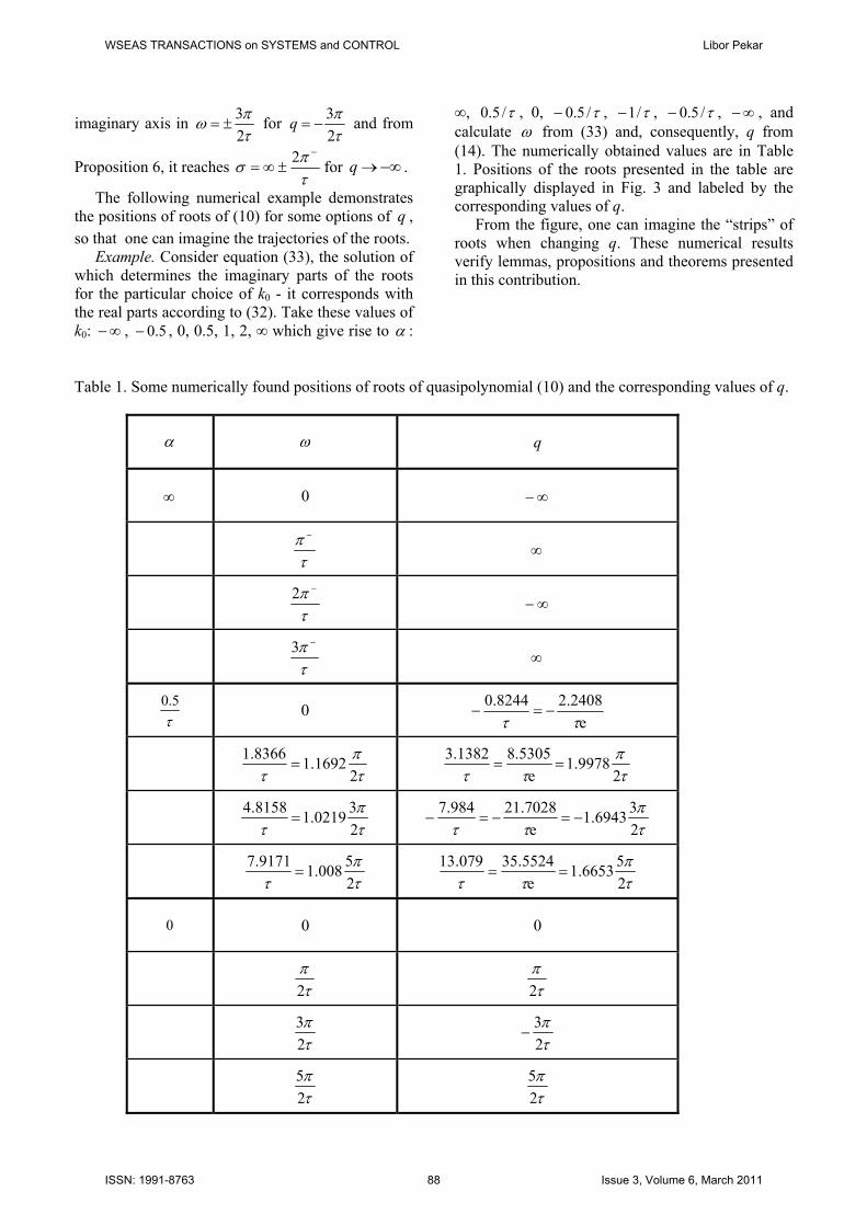
Example. Consider equation (33), the solution of which determines the imaginary parts of the roots for the particular choice of k0 - it corresponds with the real parts according to (32). Take these values of k0: , , 0, 0.5, 1, 2, ∞ which give rise to ∞− 5.0− α :

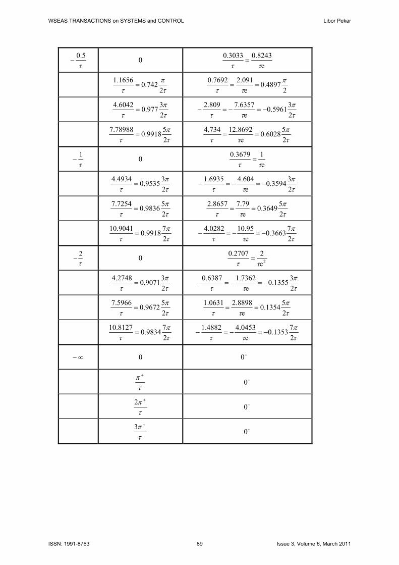
∞, τ/5.0 , 0, τ/5.0− , τ/1− , τ/5.0− , ∞− , and calculate ω from (33) and, consequently, q from (14). The numerically obtained values are in Table 1. Positions of the roots presented in the table are graphically displayed in Fig. 3 and labeled by the corresponding values of q. From the figure, one can imagine the “strips” of roots when changing q. These numerical results verify lemmas, propositions and theorems presented in this contribution.

Table 1. Some numerically found positions of roots of quasipolynomial (10) and the corresponding values of q.

ω q α

0 ∞ ∞−

τπ −

∞

τπ −2 ∞−

τπ −3 ∞

τ5.0 0

e2408.28244.0ττ

−=−

τπ

τ 21692.18366.1

= τπ

ττ 29978.1

e5305.81382.3

==

τπ

τ 230219.18158.4

= τπ

ττ 236943.1

e7028.21984.7

−=−=−

τπ

τ 25008.19171.7

= τπ

ττ 256653.1

e5524.35079.13

==

0 0 0

τπ2

τπ2

τπ

23

τπ

23

−

τπ

25

τπ

25



τ5.0

− 0 e

0.82433033.0ττ

=

τπ

τ 2742.01656.1

= 2

4897.0e

091.27692.0 πττ

==

τπ

τ 23977.06042.4

= τπ

ττ 235961.0

e6357.7809.2

−=−=−

τπ

τ 259918.078988.7

= τπ

ττ 256028.0

e8692.12734.4

==

τ1

− 0 e13679.0ττ

=

τπ

τ 239535.04934.4

= τπ

ττ 233594.0

e604.46935.1

−=−=−

τπ

τ 259836.07254.7

= τπ

ττ 253649.0

e79.78657.2

==

τπ

τ 279918.09041.10

= τπ

ττ 273663.0

e95.100282.4

−=−=−

τ2

− 0 2e22707.0ττ

=

τπ

τ 239071.02748.4

= τπ

ττ 231355.0

e7362.16387.0

−=−=−

τπ

τ 259672.05966.7

= τπ

ττ 251354.0

e8898.20631.1

==

τπ

τ 279834.08127.10

= τπ

ττ 271353.0

e0453.44882.1

−=−=−

∞− 0 −0

τπ +

+0

τπ +2 −0

τπ +3 +0



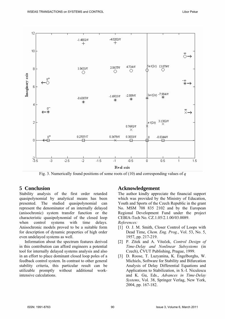
Fig. 3. Numerically found positions of some roots of (10) and corresponding values of q

5 Conclusion Stability analysis of the first order retarded quasipolynomial by analytical means has been presented. The studied quasipolynomial can represent the denominator of an internally delayed (anisochronic) system transfer function or the characteristic quasipolynomial of the closed loop when control systems with time delays. Anisochronic models proved to be a suitable form for description of dynamic properties of high order even undelayed systems as well. Information about the spectrum features derived in this contribution can afford engineers a potential tool for internally delayed systems analysis and also in an effort to place dominant closed loop poles of a feedback control system. In contrast to other general stability criteria, this particular result can be utilizable promptly without additional work-intensive calculations.

Acknowledgement The author kindly appreciate the financial support which was provided by the Ministry of Education, Youth and Sports of the Czech Republic in the grant No. MSM 708 835 2102 and by the European Regional Development Fund under the project CEBIA-Tech No. CZ.1.05/2.1.00/03.0089. References: [1] O. J. M. Smith, Closer Control of Loops with

Dead Time, Chem. Eng. Prog., Vol. 53, No. 5, 1957, pp. 217-219.

[2] P. Zítek and A. Víteček, Control Design of Time-Delay and Nonlinear Subsystems (in Czech), ČVUT Publishing, Prague, 1999.

[3] D. Roose, T. Luzyanina, K. Engelborghs, W. Michiels, Software for Stability and Bifurcation Analysis of Delay Differential Equations and Applications to Stabilization, in S.-I. Niculescu and K. Gu, Eds., Advances in Time-Delay Systems, Vol. 38, Springer Verlag, New York, 2004, pp. 167-182.



[4] V. Volterra, Sur le Théorie Mathématique des Phénomenès Héreditaires, J. Math. Pures Appl., Vol. 7, 1928, pp. 249-298.

[5] J. K. Hale and S. M. Verduyn Lunel, Introduction to Functional Differential Equations, Vol. 99 of Appl. Math. Sciences, Springer-Verlag, New York, 1993.

[6] R. Bellman and K. L. Cooke, Differential-Difference Equations, Academic Press, New York, 1963.

[7] N. N. Krasovskii, Stability of Motion, Standford University Press, Chicago, 1963.

[8] V. B. Kolmanovskii and V. R. Nosov, Stability of Functional Differential Equations, in Mathematics in Science and Engineering, Vol. 80, Academic Press, New York, 1986.

[9] H. Górecki, S. Fuksa, P. Grabowski, and A. Korytowski, Analysis and Synthesis of Time Delay Systems, PWN, Warszawa, 1989.

[10] A. Z. Manitius and A. W. Olbrot, Finite Spectrum Assignment Problem for Systems with Delays, IEEE Trans. Aut. Control, Vol. 24, No. 4, 1979, pp. 541-553.

[11] L. E. El’sgol’ts and S. B. Norkin, Introduction to the Theory and Application of Differential Equations with Deviated Arguments, Academic Press, New York, 1973.

[12] P. Zítek and J. Hlava, Anisochronic Internal Model Control of Time-Delay Systems, Control Engng Pract., Vol. 9, No. 5, 2001, pp. 501-516.

[13] P. Zítek, Frequency Domain Synthesis of Hereditary Control Systems via Anisochronic State Space, Int. J. Control, Vol. 66, No. 4, 1997, pp. 539-556.

[14] L. Pekař, R. Prokop, and P. Dostálek, Circuit Heating Plant Model with Internal Delays, WSEAS Trans. Systems, Vol. 8, Issue 9, September 2009, pp. 1093-1104.

[15] C. Roduner and H.-P. Geering, Modellbasierte Mehrgroessen-Regulung eines Ottomotors unter Berueckichtigung der Totzeiten (Model-Based Multivariable Control of a Gasoline Engine under Consideration of Receiver Dead Times), Automatisierungstechnik, Vol. 44, 1996, pp. 314-321.

[16] W. Findensen, J. Pulaczewski, and A. Manitius, Multilevel Optimization and Dynamic Coordination of Mass Flows in a Beet Sugar Plant, Automatica, Vol. 6, 1970, pp. 581-589.

[17] J. Morávka and K. Michálek, Anisochronous Model of the Metallurgical RH Process, Trans. of the VŠB – Technical University of Ostrava,

Mechanical Series, Vol. 14, No. 2, 2008, pp. 91-96.

[18] L. S. Pontryagin, On the Zeros of Some Elementary Transcendental Functions, Izvestiya Akademii Nauk SSSR, Vol. 6, 1942, pp. 115-131.

[19] J. - P. Richard, Time-delay Systems: an Overview of Some Recent Advances and Open problems, Automatica, Vol. 39, Issue 10, 2003, pp. 1667-1694.

[20] W. Michiels and S. I. Nicolescu, Stability and Stabilization of Time Delay Systems: An Eigenvalue Based Approach, Vol. 12 of SIAM Advan. in Design and Control, Society for Industrial Mathematics, New York, 2007.

[21] T. Hashimoto and T. Amemyia, Stabilization of Linear Time-Varying Uncertain Delay Systems with Double Triangular Configuration, WSEAS Trans. Systems and Control, Vol. 4, Issue 9, 2009, pp. 465-475.

[22] P. Zítek, Anisochronic Modelling and Stability Criterion of Hereditary systems, Problems of Control and Information Theory, Vol. 15, No. 6, 1986, pp. 413-423.

[23] J. K. Hale, S. M. Verduyn Lunel, Strong Stabilization of Neutral Functional Differential Equations, IMA Journal of Math. Control and Information, Vol. 19, Issue 1-2, 2002, pp. 5-23.

[24] N. Olgac, R. Sipahi, An Exact Method for the Stability Analysis of Time Delay LTI Systems, IEEE Transaction on Automatic Control, Vol. 47, No. 5, 2002, pp. 793-797.

[25] W. Michiels, T. Vyhlídal, An Eigenvalue Based Approach for the Stabilization of Linear Time-Delay Systems of Neutral Type, Automatica, Vol. 41, Issue 6, 2005, pp. 991-998.

[26] Y. Zhang, Spectrum of A Class of Delay Differential Equations and Its Solution Expansion, WSEAS Trans. Mathematics, Vol. 10, Issue 5, 2011, pp. 169-180.

[27] L. Pekař and R. Prokop, An Approach for Relay Based Identification of Anisochronic Models, in Proc. 27th IASTED int. Confer. Modeling, Identification and Control, Innsbruck, 2008.

[28] T. Vyhlídal and P. Zítek, Control System Design Based on a Universal First Order Model with Time Delays. Acta Polytechnica, 2001, Vol. 44, No. 4-5, pp. 49-53.

[29] W. Michiels, K. Engelbourghs, D. Roose, and D. Dochain, Sensitivity to Infinitesimal Delays in Neutral Equations, SIAM J. Control, 2001, Vol. 40, No. 4, pp. 1134-1158.



Documents

Root Locus Analysis of a Retarded Quasipolynomial