Ad Hoc Networks 7 (2009) 219–229

Contents lists available at ScienceDirect

Ad Hoc Networks

journal homepage: www.elsevier .com/locate /adhoc

Routing based on delivery distributions in predictable disruptiontolerant networks q

Jean-Marc Franc�ois *, Guy Leduc 1

Research Unit in Networking, Department of Electrical Engineering and Computer Science, Institut Montefiore, Sart-Tilman, Université de Liège, Liège, Belgium

a r t i c l e i n f o

Article history:Received 9 January 2008Accepted 2 February 2008Available online 17 March 2008

Keywords:Delivery guaranteesDisruption tolerant networks (DTNs)Bellman–Ford algorithmMobility prediction

1570-8705/$ - see front matter � 2008 Elsevier B.Vdoi:10.1016/j.adhoc.2008.02.006

q This work has been partially supported by the Belthe framework of the IAP program (Motion P5/11European E-Next NoE and IST-FET ANA project.

* Corresponding author.E-mail addresses: francois@run.montefiore.ulg.a

leduc@run.montefiore.ulg.ac.be (G. Leduc).1 Tel.: +32 4 3662698.

a b s t r a c t

This article studies disruption tolerant networks (DTNs) where each node knows the prob-abilistic distribution of contacts with other nodes. It proposes a framework that allows oneto formalize the behaviour of such a network. It generalizes extreme cases that have beenstudied before where (a) either nodes only know their contact frequency with each other or(b) they have a perfect knowledge of who meets who and when. This paper then gives anexample of how this framework can be used; it shows how one can find a packet forward-ing algorithm optimized to meet the ‘delay/bandwidth consumption’ tradeoff: packets areduplicated so as to (statistically) guarantee a given delay or delivery probability, but nottoo much so as to reduce the bandwidth, energy, and memory consumption.

� 2008 Elsevier B.V. All rights reserved.

1. Introduction

Disruption (or delay) tolerant networks (DTNs, [1]) havebeen the subject of much research activity in the last fewyears, pushing further the concept of ad hoc networks. Likead hoc networks, DTNs are infrastructureless, thus thepackets are relayed from one node to the next until theyreach their destination. Moreover, in DTNs node clusterscan be completely disconnected from the rest of the net-work. In this case, nodes must buffer the packets and waituntil node mobility changes the network’s topology, allow-ing the packets to be finally delivered.

A network of Bluetooth-enabled PDAs, a village inter-mittently connected via low Earth orbiting satellites, oreven an interplanetary Internet [2] are examples of disrup-tion tolerant networks.

. All rights reserved.

gian Science Policy inproject) and by the

c.be (J.-M. Franc�ois),

The atomic data unit is a group of packets to be deliv-ered together. In DTN parlance, it is called a message or abundle; we use the latter in the following.

Routing in such networks is particularly challengingsince it requires to take into account the uncertainty ofmobiles movements. The first methods that have been pro-posed in the literature are pretty radical and propose toforward bundles in an ‘‘epidemic” way [3–5], i.e., to copythem each time a new node is encountered. This methodof course results in optimum delays and delivery probabil-ities, at the expense of an extremely high consumption ofbandwidth (and, thus, energy) and memory. To mitigatethose shortcomings, the epidemic routing has been en-hanced using heuristics that allow the propagation of bun-dles to a subset of all the nodes [6–8].

Since node’s buffer memory is not unlimited, a cachemechanism has been proposed, where the most interestingbundles are kept (i.e. those that are likely to reach theirdestination soon) and the others are discarded when thecache is full [9–14]. Those schemes must thus guess whena bundle will reach its destination, which is most of thetime computed thanks to frequency contact estimation(which reflects the probability that two given nodes meetin the future; this probability is most of the time consid-ered time-invariant).

220 J.-M. Franc�ois, G. Leduc / Ad Hoc Networks 7 (2009) 219–229

Few papers explore how the expected delay could bemore precisely estimated (notable exceptions are[15,16]). It has been proved [17] that a perfect knowledgeof the future node meetings allows the computation of anoptimal bundle routing.

This short overview emphasizes two shortcomings:

� Certain networks might be highly predictable (e.g. nodesare satellites and links appear and vanish as they revolvearound their planet), others are much more chaotic. Pre-vious work suppose either that nodes contacts are per-fectly deterministic and known in advance, or thatonly the contact frequency is known for each pair ofnodes. In this paper, we propose to suppose that eachnode knows a probability distribution of contacts inthe (near) future. We introduce a framework which gen-eralizes those extreme cases and formalizes the nodescontact predictability. It allows one to compute theexpected impact of a particular bundle forwardingstrategy.

� Ref. [5] underlines the tradeoff between bundle deliveryguarantees and bandwidth/energy consumption: copy-ing the bundles is costly since, in mobile networks, thoseresources are both scarce. Current schemes use a cachemechanism that ensures each node only receives themost relevant bundles, which somehow mitigates thisproblem, but does not provide any rationale, exceptthe need to cope with mobiles limited memory. We pro-pose to use the above-mentioned framework to routethe bundles according to the delivery or delay guaran-tees required by the user, thus only duplicating packetswhen it is beneficial.

Most of the ideas presented in this article have beenfirst published in [18]; this article is an extended versionof this paper.

This paper is organised as follows. Section 2 presents away to model the contacts between the nodes of a predict-able network. Sections 2 and 4 show how the end-to-enddelay of bundles can be predicted. Sections 5 and 6 give arouting algorithm that allows one to deliver bundles soas to meet a given guarantee. Section 7 concludes.

2. Predictable future contacts

The network is composed of a finite set of wirelessnodes N that can move and thus, from time to time, comeinto contact.

In the sequel, a contact between two nodes happenwhen those nodes have setup a bi-directional wireless linkbetween them. A contact is always considered long enoughto allow all the required data exchanges to take place.2

2.1. Contact profiles

We expect the mobiles motion to be, to a certain extent,predictable, yet obviously the degree of predictability var-

2 This is a major difference with [17] which does not neglect bundletransmission times.

ies from one network to another. Sometimes nodes motionis known in advance because they must stick to a givenschedule (e.g. a network of buses) or because their trajec-tory can easily be modelled (e.g. nodes embedded in asatellite). Other networks are less predictable, yet not to-tally random: colleagues could be pretty sure to meetevery day during working hours, without any other timeguarantee. Mobile nodes behaviour could also be learntautomatically so as to extract cyclical contact patterns.

We therefore suppose that each node pair fa; bg �N

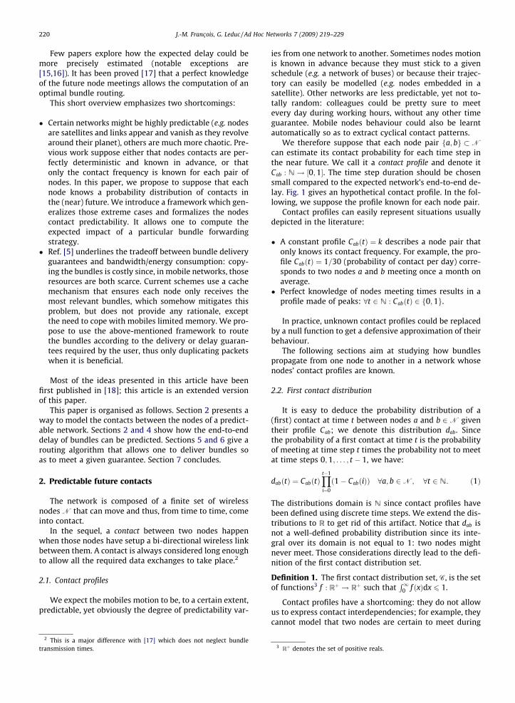
can estimate its contact probability for each time step inthe near future. We call it a contact profile and denote itCab : N! ½0;1�. The time step duration should be chosensmall compared to the expected network’s end-to-end de-lay. Fig. 1 gives an hypothetical contact profile. In the fol-lowing, we suppose the profile known for each node pair.

Contact profiles can easily represent situations usuallydepicted in the literature:

� A constant profile CabðtÞ ¼ k describes a node pair thatonly knows its contact frequency. For example, the pro-file CabðtÞ ¼ 1=30 (probability of contact per day) corre-sponds to two nodes a and b meeting once a month onaverage.

� Perfect knowledge of nodes meeting times results in aprofile made of peaks: 8t 2 N : CabðtÞ 2 f0;1g.

In practice, unknown contact profiles could be replacedby a null function to get a defensive approximation of theirbehaviour.

The following sections aim at studying how bundlespropagate from one node to another in a network whosenodes’ contact profiles are known.

2.2. First contact distribution

It is easy to deduce the probability distribution of a(first) contact at time t between nodes a and b 2N giventheir profile Cab; we denote this distribution dab. Sincethe probability of a first contact at time t is the probabilityof meeting at time step t times the probability not to meetat time steps 0;1; . . . ; t � 1, we have:

dabðtÞ ¼ CabðtÞYt�1

i¼0

ð1� CabðiÞÞ 8a; b 2N; 8t 2 N: ð1Þ

The distributions domain is N since contact profiles havebeen defined using discrete time steps. We extend the dis-tributions to R to get rid of this artifact. Notice that dab isnot a well-defined probability distribution since its inte-gral over its domain is not equal to 1: two nodes mightnever meet. Those considerations directly lead to the defi-nition of the first contact distribution set.

Definition 1. The first contact distribution set, C, is the setof functions3 f : Rþ ! Rþ such that

R10 f ðxÞdx 6 1.

Contact profiles have a shortcoming: they do not allowus to express contact interdependencies; for example, theycannot model that two nodes are certain to meet during

3 Rþ denotes the set of positive reals.

0

5

10

15

20

25

30

0 5 10 15 20 25 30

Pro

babi

lity

(%)

Time (days)

Fig. 1. Contact profile of a node pair over a month: example. The height of a bar gives the probability that two nodes meet (at least once) during thecorresponding 12-h time period. Here, nodes are supposed to meet at the beginning of each week, but the exact day is unknown.

0

5

10

15

20

25

30

35

40

45

0 5 10 15 20 25 30

Pro

babi

lity

dens

ity (

%/d

ay)

Time (days)

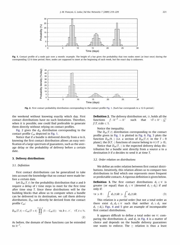
Fig. 2. First contact probability distribution corresponding to the contact profile Fig. 1. (Each bar corresponds to a 12-h period.)

J.-M. Franc�ois, G. Leduc / Ad Hoc Networks 7 (2009) 219–229 221

the weekend without knowing exactly which day. Firstcontact distributions have no such limitations. Therefore,when it is possible, one could find preferable to generatethem directly without relying on contact profiles.

Fig. 2 gives the dab distribution corresponding to thecontact profile Cab depicted in Fig. 1.

Notice that if a bundle is delivered directly from a to b,knowing the first contact distribution allows an easy veri-fication of a large spectrum of guarantees, such as the aver-age delay or the probability of delivery before a certaindate.

3. Delivery distributions

3.1. Definition

First contact distributions can be generalized to takeinto account the knowledge that no contact were made be-fore a certain date.

Let DabðT; tÞ be the probability distribution that a and brequire a delay of t time steps to meet for the first timeafter time step T. Since these distributions will be thebuilding blocks that allow us to compute when a bundlecan be delivered to its destination, we call them deliverydistributions. Dab can directly be derived from the contactprofile Cab:

DabðT; tÞ ¼ CabðT þ tÞYTþt�1

i¼T

ð1� CabðiÞÞ 8a;b 2N; 8T; t 2N:

ð2Þ

As before, the domain of these functions can be extendedto Rþ

2.

Definition 2. The delivery distribution set, D, holds all thefunctions f : Rþ

2 ! Rþ such that 8T 2 Rþ :R1

0f ðT; xÞdx 6 1.

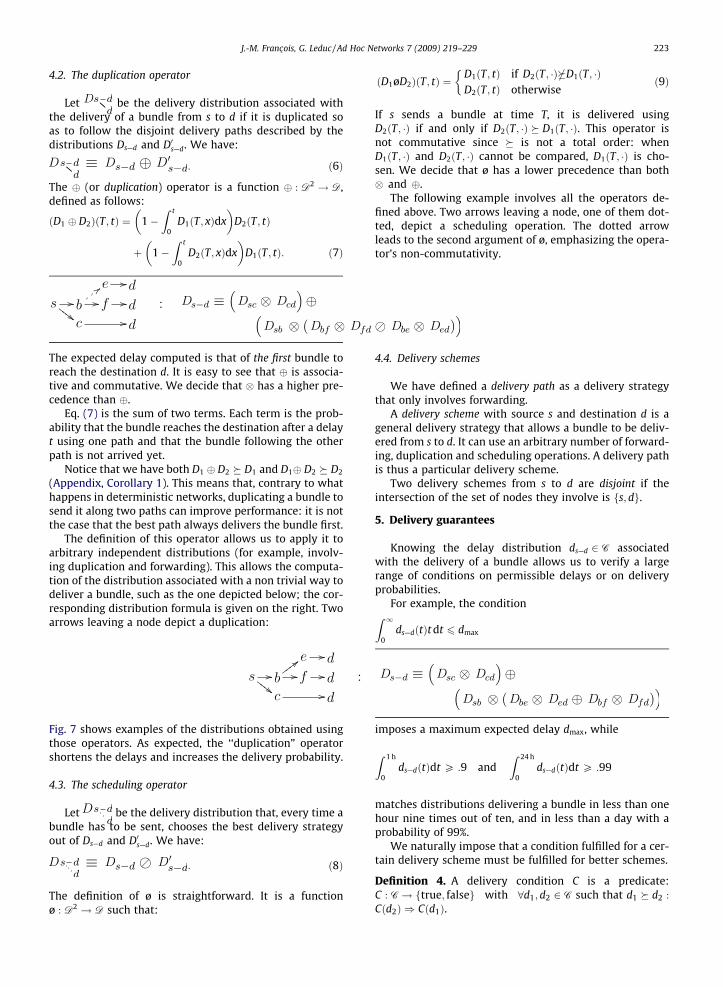
Notice the inequality.The DabðT; tÞ distribution corresponding to the contact

profile given in Fig. 1 is plotted in Fig. 6. Fig. 3 plots thefunction Dabð9; �Þ (i.e. a section of DabðT; tÞ in the T ¼ 9plane); the DðT; �Þ functions of course belong to Cð8T P 0Þ.

Notice that DabðT; �Þ is the expected delivery delay dis-tribution for a bundle sent directly from a source a to adestination b if a decides to send it at time T.

3.2. Order relation on distributions

We define an order relation between first contact distri-butions. Intuitively, this relation allows us to compare twodistributions to find which one represents more frequentor predictable contacts. A rigorous definition is given below.

Definition 3. The first contact distributions d1 2 C isgreater (or equal) than d2 2 C (denoted d1 � d2) if andonly if:

8x P 0 :

Z x

0d1ðtÞdt P

Z x

0d2ðtÞdt: ð3Þ

This relation is a partial order (but not a total order asthere exist d1; d2 2 C such that neither d1 � d2 nord1 � d2). Figs. 4 and 5 give an example of incomparablefirst contact distributions.

It appears difficult to define a total order on C: com-paring the distributions d1 and d2 in Fig. 4 is a matter ofchoice and depends on the bundle delivery guaranteesone wants to enforce. The � relation is thus a least

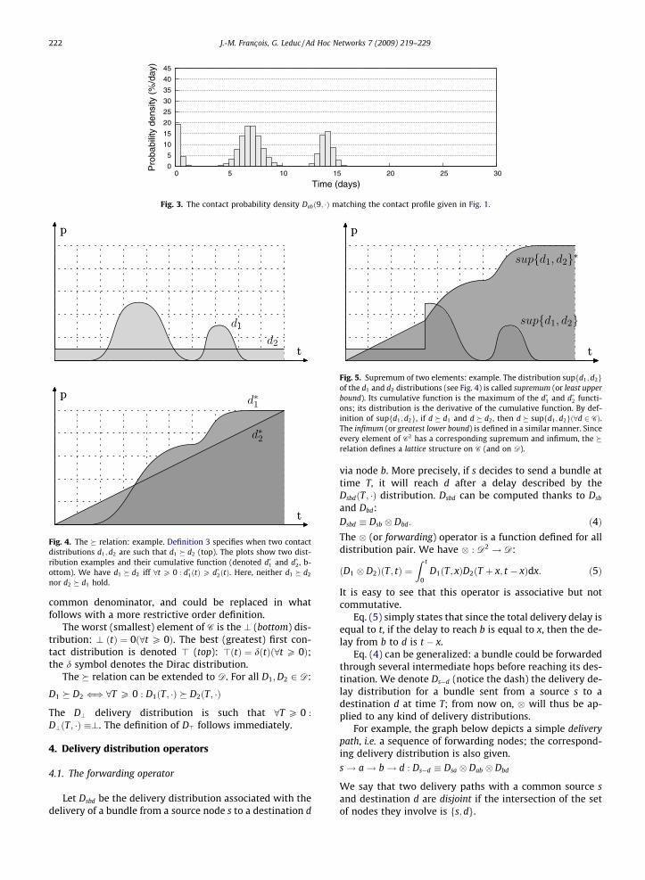
Fig. 4. The � relation: example. Definition 3 specifies when two contactdistributions d1;d2 are such that d1 � d2 (top). The plots show two dist-ribution examples and their cumulative function (denoted d�1 and d�2, b-ottom). We have d1 � d2 iff 8t P 0 : d�1ðtÞP d�2ðtÞ. Here, neither d1 � d2

nor d2 � d1 hold.

0

5

10

15

20

25

30

35

40

45

0 5 10 15 20 25 30

Pro

babi

lity

dens

ity (

%/d

ay)

Time (days)

Fig. 3. The contact probability density Dabð9; �Þ matching the contact profile given in Fig. 1.

Fig. 5. Supremum of two elements: example. The distribution supfd1;d2gof the d1 and d2 distributions (see Fig. 4) is called supremum (or least upperbound). Its cumulative function is the maximum of the d�1 and d�2 functi-ons; its distribution is the derivative of the cumulative function. By def-inition of supfd1; d2g, if d � d1 and d � d2, then d � supfd1; d2gð8d 2 CÞ.The infimum (or greatest lower bound) is defined in a similar manner. Sinceevery element of C2 has a corresponding supremum and infimum, the �relation defines a lattice structure on C (and on D).

222 J.-M. Franc�ois, G. Leduc / Ad Hoc Networks 7 (2009) 219–229

common denominator, and could be replaced in whatfollows with a more restrictive order definition.

The worst (smallest) element of C is the ? (bottom) dis-tribution: ? ðtÞ ¼ 0ð8t P 0Þ. The best (greatest) first con-tact distribution is denoted > (top): >ðtÞ ¼ dðtÞð8t P 0Þ;the d symbol denotes the Dirac distribution.

The � relation can be extended to D. For all D1;D2 2 D:

D1 � D2 () 8T P 0 : D1ðT; �Þ � D2ðT; �Þ

The D? delivery distribution is such that 8T P 0 :

D?ðT; �Þ ?. The definition of D> follows immediately.

4. Delivery distribution operators

4.1. The forwarding operator

Let Dsbd be the delivery distribution associated with thedelivery of a bundle from a source node s to a destination d

via node b. More precisely, if s decides to send a bundle attime T, it will reach d after a delay described by theDsbdðT; �Þ distribution. Dsbd can be computed thanks to Dsb

and Dbd:Dsbd Dsb Dbd: ð4ÞThe (or forwarding) operator is a function defined for alldistribution pair. We have : D2 ! D:

ðD1 D2ÞðT; tÞ ¼Z t

0D1ðT; xÞD2ðT þ x; t � xÞdx: ð5Þ

It is easy to see that this operator is associative but notcommutative.

Eq. (5) simply states that since the total delivery delay isequal to t, if the delay to reach b is equal to x, then the de-lay from b to d is t � x.

Eq. (4) can be generalized: a bundle could be forwardedthrough several intermediate hops before reaching its des-tination. We denote Ds—d (notice the dash) the delivery de-lay distribution for a bundle sent from a source s to adestination d at time T; from now on, will thus be ap-plied to any kind of delivery distributions.

For example, the graph below depicts a simple deliverypath, i.e. a sequence of forwarding nodes; the correspond-ing delivery distribution is also given.s! a! b! d : Ds—d Dsa Dab Dbd

We say that two delivery paths with a common source sand destination d are disjoint if the intersection of the setof nodes they involve is fs; dg.

J.-M. Franc�ois, G. Leduc / Ad Hoc Networks 7 (2009) 219–229 223

4.2. The duplication operator

Let be the delivery distribution associated withthe delivery of a bundle from s to d if it is duplicated soas to follow the disjoint delivery paths described by thedistributions Ds—d and D0s—d. We have:

: ð6Þ

The � (or duplication) operator is a function � : D2 ! D,defined as follows:

ðD1 � D2ÞðT; tÞ ¼ 1�Z t

0D1ðT; xÞdx

� �D2ðT; tÞ

þ 1�Z t

0D2ðT; xÞdx

� �D1ðT; tÞ: ð7Þ

The expected delay computed is that of the first bundle toreach the destination d. It is easy to see that � is associa-tive and commutative. We decide that has a higher pre-cedence than �.

Eq. (7) is the sum of two terms. Each term is the prob-ability that the bundle reaches the destination after a delayt using one path and that the bundle following the otherpath is not arrived yet.

Notice that we have both D1 � D2 � D1 and D1� D2 � D2

(Appendix, Corollary 1). This means that, contrary to whathappens in deterministic networks, duplicating a bundle tosend it along two paths can improve performance: it is notthe case that the best path always delivers the bundle first.

The definition of this operator allows us to apply it toarbitrary independent distributions (for example, involv-ing duplication and forwarding). This allows the computa-tion of the distribution associated with a non trivial way todeliver a bundle, such as the one depicted below; the cor-responding distribution formula is given on the right. Twoarrows leaving a node depict a duplication:

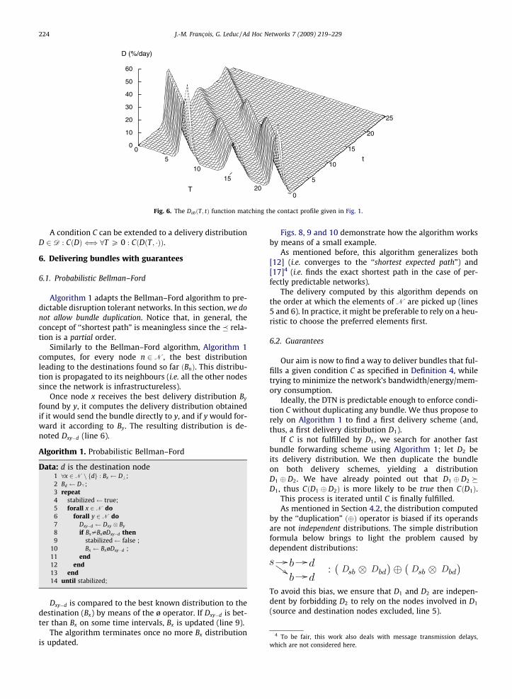
Fig. 7 shows examples of the distributions obtained usingthose operators. As expected, the ‘‘duplication” operatorshortens the delays and increases the delivery probability.

4.3. The scheduling operator

Let be the delivery distribution that, every time abundle has to be sent, chooses the best delivery strategyout of Ds—d and D0s—d. We have:

: ð8Þ

The definition of ø is straightforward. It is a functionø : D2 ! D such that:

ðD1øD2ÞðT; tÞ ¼D1ðT; tÞ if D2ðT; �Þ†D1ðT; �ÞD2ðT; tÞ otherwise

�ð9Þ

If s sends a bundle at time T, it is delivered usingD2ðT; �Þ if and only if D2ðT; �Þ � D1ðT; �Þ. This operator isnot commutative since � is not a total order: whenD1ðT; �Þ and D2ðT; �Þ cannot be compared, D1ðT; �Þ is cho-sen. We decide that ø has a lower precedence than both and �.

The following example involves all the operators de-fined above. Two arrows leaving a node, one of them dot-ted, depict a scheduling operation. The dotted arrowleads to the second argument of ø, emphasizing the opera-tor’s non-commutativity.

4.4. Delivery schemes

We have defined a delivery path as a delivery strategythat only involves forwarding.

A delivery scheme with source s and destination d is ageneral delivery strategy that allows a bundle to be deliv-ered from s to d. It can use an arbitrary number of forward-ing, duplication and scheduling operations. A delivery pathis thus a particular delivery scheme.

Two delivery schemes from s to d are disjoint if theintersection of the set of nodes they involve is fs; dg.

5. Delivery guarantees

Knowing the delay distribution ds—d 2 C associatedwith the delivery of a bundle allows us to verify a largerange of conditions on permissible delays or on deliveryprobabilities.

For example, the conditionZ 1

0ds—dðtÞt dt 6 dmax

imposes a maximum expected delay dmax, while

Z 1 h

0ds—dðtÞdt P :9 and

Z 24 h

0ds—dðtÞdt P :99

matches distributions delivering a bundle in less than onehour nine times out of ten, and in less than a day with aprobability of 99%.

We naturally impose that a condition fulfilled for a cer-tain delivery scheme must be fulfilled for better schemes.

Definition 4. A delivery condition C is a predicate:C : C! ftrue; falseg with 8d1; d2 2 C such that d1 � d2 :

Cðd2Þ ) Cðd1Þ.

0

5

10

15

20T 0

5

10

15

20

25

t

0

10

20

30

40

50

60

D (%/day)

Fig. 6. The DabðT; tÞ function matching the contact profile given in Fig. 1.

224 J.-M. Franc�ois, G. Leduc / Ad Hoc Networks 7 (2009) 219–229

A condition C can be extended to a delivery distributionD 2 D : CðDÞ () 8T P 0 : CðDðT; �ÞÞ.

6. Delivering bundles with guarantees

6.1. Probabilistic Bellman–Ford

Algorithm 1 adapts the Bellman–Ford algorithm to pre-dictable disruption tolerant networks. In this section, we donot allow bundle duplication. Notice that, in general, theconcept of ‘‘shortest path” is meaningless since the � rela-tion is a partial order.

Similarly to the Bellman–Ford algorithm, Algorithm 1computes, for every node n 2N, the best distributionleading to the destinations found so far ðBnÞ. This distribu-tion is propagated to its neighbours (i.e. all the other nodessince the network is infrastructureless).

Once node x receives the best delivery distribution By

found by y, it computes the delivery distribution obtainedif it would send the bundle directly to y, and if y would for-ward it according to By. The resulting distribution is de-noted Dxy�d (line 6).

Algorithm 1. Probabilistic Bellman–Ford

Data: d is the destination node1 8x 2N n fdg : Bx D?;2 Bd D>;3 repeat4 stabilized true;5 forall x 2N do6 forall y 2N do7 Dxy�d Dxy By

8 if Bx–BxøDxy�d then9 stabilized false ;

10 Bx BxøDxy�d ;11 end12 end13 end14 until stabilized;

4 To be fair, this work also deals with message transmission delays,which are not considered here.

Dxy�d is compared to the best known distribution to thedestination (Bx) by means of the ø operator. If Dxy�d is bet-ter than Bx on some time intervals, Bx is updated (line 9).

The algorithm terminates once no more Bx distributionis updated.

Figs. 8, 9 and 10 demonstrate how the algorithm worksby means of a small example.

As mentioned before, this algorithm generalizes both[12] (i.e. converges to the ‘‘shortest expected path”) and[17]4 (i.e. finds the exact shortest path in the case of per-fectly predictable networks).

The delivery computed by this algorithm depends onthe order at which the elements of N are picked up (lines5 and 6). In practice, it might be preferable to rely on a heu-ristic to choose the preferred elements first.

6.2. Guarantees

Our aim is now to find a way to deliver bundles that ful-fills a given condition C as specified in Definition 4, whiletrying to minimize the network’s bandwidth/energy/mem-ory consumption.

Ideally, the DTN is predictable enough to enforce condi-tion C without duplicating any bundle. We thus propose torely on Algorithm 1 to find a first delivery scheme (and,thus, a first delivery distribution D1).

If C is not fulfilled by D1, we search for another fastbundle forwarding scheme using Algorithm 1; let D2 beits delivery distribution. We then duplicate the bundleon both delivery schemes, yielding a distributionD1 � D2. We have already pointed out that D1 � D2 �D1, thus CðD1 � D2Þ is more likely to be true then CðD1Þ.

This process is iterated until C is finally fulfilled.As mentioned in Section 4.2, the distribution computed

by the ‘‘duplication” ð�Þ operator is biased if its operandsare not independent distributions. The simple distributionformula below brings to light the problem caused bydependent distributions:

To avoid this bias, we ensure that D1 and D2 are indepen-dent by forbidding D2 to rely on the nodes involved in D1

(source and destination nodes excluded, line 5).

0

20

40

60

80

100

0 5 10 15 20 25 30

Pro

babi

lity

(%)

Time (days)

t

T0

10

0 10 20 30

0 5

10 15

20 25

T 0

5

10

15

20

25

t

0

20

40

60

80

100

120

140

D (%/day)

0 5

10 15

20 25

T 0

5

10

15

20

25

t

0

50

100

150

200

250

D (%/day)

Fig. 7. Forwarding () and duplication ð�Þ operators: example. We denote D1 the delivery distribution depicted in Fig. 6. The top part of this figure depicts acontact profile (top) and the associated delivery distribution D2 (dark squares represent a probability equal to 1). The top 3D plot depicts D1 D2, thebottom one D1 � D2. A contact profile and the associated delivery distribution D2.

J.-M. Franc�ois, G. Leduc / Ad Hoc Networks 7 (2009) 219–229 225

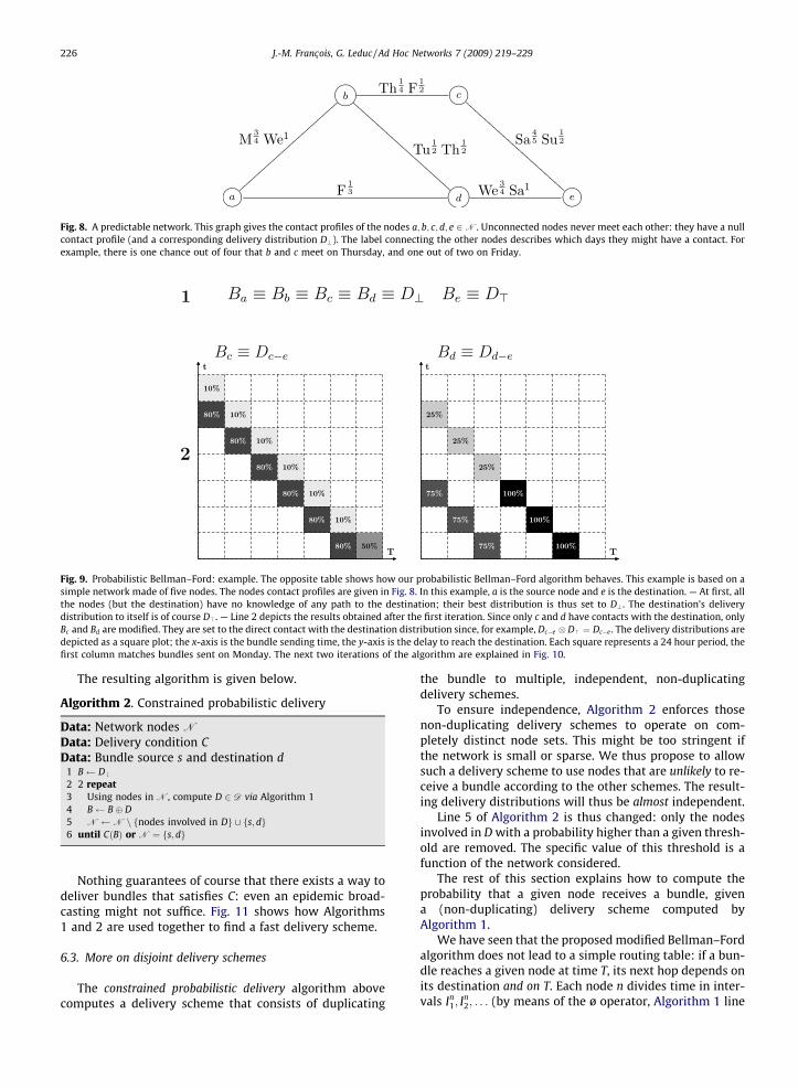
Fig. 9. Probabilistic Bellman–Ford: example. The opposite table shows how our probabilistic Bellman–Ford algorithm behaves. This example is based on asimple network made of five nodes. The nodes contact profiles are given in Fig. 8. In this example, a is the source node and e is the destination. — At first, allthe nodes (but the destination) have no knowledge of any path to the destination; their best distribution is thus set to D? . The destination’s deliverydistribution to itself is of course D>. — Line 2 depicts the results obtained after the first iteration. Since only c and d have contacts with the destination, onlyBc and Bd are modified. They are set to the direct contact with the destination distribution since, for example, Dc�e D> ¼ Dc�e . The delivery distributions aredepicted as a square plot; the x-axis is the bundle sending time, the y-axis is the delay to reach the destination. Each square represents a 24 hour period, thefirst column matches bundles sent on Monday. The next two iterations of the algorithm are explained in Fig. 10.

Fig. 8. A predictable network. This graph gives the contact profiles of the nodes a; b; c;d; e 2N. Unconnected nodes never meet each other: they have a nullcontact profile (and a corresponding delivery distribution D?). The label connecting the other nodes describes which days they might have a contact. Forexample, there is one chance out of four that b and c meet on Thursday, and one out of two on Friday.

226 J.-M. Franc�ois, G. Leduc / Ad Hoc Networks 7 (2009) 219–229

The resulting algorithm is given below.

Algorithm 2. Constrained probabilistic delivery

Data: Network nodes N

Data: Delivery condition CData: Bundle source s and destination d

1 B D?2 2 repeat3 Using nodes in N, compute D 2 D via Algorithm 14 B B� D5 N N n fnodes involved in Dg [ fs; dg6 until CðBÞ or N ¼ fs; dg

Nothing guarantees of course that there exists a way todeliver bundles that satisfies C: even an epidemic broad-casting might not suffice. Fig. 11 shows how Algorithms1 and 2 are used together to find a fast delivery scheme.

6.3. More on disjoint delivery schemes

The constrained probabilistic delivery algorithm abovecomputes a delivery scheme that consists of duplicating

the bundle to multiple, independent, non-duplicatingdelivery schemes.

To ensure independence, Algorithm 2 enforces thosenon-duplicating delivery schemes to operate on com-pletely distinct node sets. This might be too stringent ifthe network is small or sparse. We thus propose to allowsuch a delivery scheme to use nodes that are unlikely to re-ceive a bundle according to the other schemes. The result-ing delivery distributions will thus be almost independent.

Line 5 of Algorithm 2 is thus changed: only the nodesinvolved in D with a probability higher than a given thresh-old are removed. The specific value of this threshold is afunction of the network considered.

The rest of this section explains how to compute theprobability that a given node receives a bundle, givena (non-duplicating) delivery scheme computed byAlgorithm 1.

We have seen that the proposed modified Bellman–Fordalgorithm does not lead to a simple routing table: if a bun-dle reaches a given node at time T, its next hop depends onits destination and on T. Each node n divides time in inter-vals In

1; In2; . . . (by means of the ø operator, Algorithm 1 line

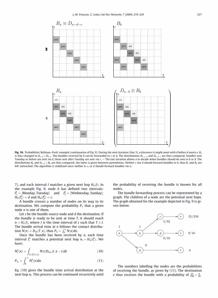
Fig. 10. Probabilistic Bellman–Ford: example (continuation of Fig. 9). During the next iteration (line 3), a discovers it might meet with d before d meets e. Ba

is thus changed to Da�d Dd�e . The bundles received by b can be forwarded to c or d. The distributions Db�c�e and Db�d�e are thus compared; bundles sentTuesday or before are sent via d, those sent after Tuesday are sent via c. — The last iteration allows a to decide when bundles should be sent to b or d. Thedistributions Ba and Da�b Bb are thus compared; the latter is given between parentheses. Neither c nor d should forward bundles to b, thus Bc and Bd areleft untouched. The algorithm is stabilized since neither b, c, or d should forward bundles via a.

J.-M. Franc�ois, G. Leduc / Ad Hoc Networks 7 (2009) 219–229 227

7), and each interval I matches a given next hop HnðIÞ. Inthe example Fig. 9, node b has defined two intervals:Ib1 ¼ ½Monday;Tuesday� and Ib

2 ¼ ½Wednesday; Sunday�;HbðIb

1Þ ¼ d and HbðIb2Þ ¼ c.

A bundle crosses a number of nodes on its way to itsdestination. We compute the probability Pn that a givennode n is one of them.

Let s be the bundle source node and d the destination. Ifthe bundle is ready to be sent at time T, it should reachn ¼ HsðIÞ, where I is the time interval of s such that T 2 I.The bundle arrival time at n follows the contact distribu-tion NðxÞ ¼ DsnðT; xÞ, thus Pn ¼

R10 NðxÞdx.

Once the bundle has been received by n, each timeinterval In

i matches a potential next hop ni ¼ HnðIni Þ. We

have:

Nni ðxÞ ¼

Zft2In

i jt6xgNðtÞDnni

ðt; x� tÞdt: ð10Þ

Pni¼Z 1

0Nn

i ðxÞdx: ð11Þ

Eq. (10) gives the bundle time arrival distribution at thenext hop ni. This process can be continued recursively until

the probability of receiving the bundle is known for allnodes.

The bundle forwarding process can be represented by agraph. The children of a node are the potential next hops.The graph obtained for the example depicted in Fig. 9 is gi-ven below.

The numbers labelling the nodes are the probabilitiesof receiving the bundle, as given by (11). The destinatione thus receives the bundle with a probability of 25

256þ 916.

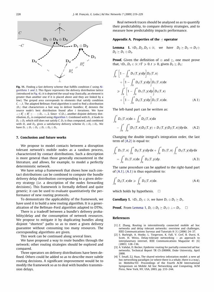
Fig. 11. Finding a fast delivery scheme that fulfills condition C using Al-gorithms 1 and 2. This figure represents the delivery distribution lattice(introduced in Fig. 4); it is depicted the usual way (basically, an element isgreater than another one if it is placed above and they are linked by aline). The greyed area corresponds to elements that satisfy conditionC. —,1. The adapted Bellman–Ford algorithm is used to find a distributionðD1Þ that characterizes a fast way to deliver bundles; Bi

s denotes thesource node’s best distribution found after i iterations. We have?� B1

s � B2s � � � � � D1. —, 2. Since :CðD1Þ, another disjoint delivery dist-

ribution, D2, is computed using Algorithm 1. Combined with D1, it leads toD1 � D2 which still does not satisfy C. D3 is thus computed, and combinedwith D1 and D2, gives a satisfactory delivery scheme D1 � D2 � D3. Wehave D1 � D1 � D2 � D1 � D2 � D3.

228 J.-M. Franc�ois, G. Leduc / Ad Hoc Networks 7 (2009) 219–229

7. Conclusion and future works

We propose to model contacts between a disruptiontolerant network’s mobile nodes as a random process,characterized by contact distributions. Such a descriptionis more general than those generally encountered in theliterature, and allows, for example, to model a perfectlydeterministic network.

We have setup a framework that shows how such con-tact distributions can be combined to compute the bundledelivery delay distribution corresponding to a given deliv-ery strategy (i.e. a description of the nodes forwardingdecisions). This framework is formally defined and quitegeneric; it can be used to evaluate quantitatively the per-formance of new routing protocols.

To demonstrate the applicability of the framework, wehave used it to build a new routing algorithm. It is a gener-alization of the Bellman–Ford algorithm adapted to DTNs.

There is a tradeoff between a bundle’s delivery proba-bility/delay and the consumption of network resources.We propose to mitigate it by duplicating bundles alongdisjoint ‘‘shortest” paths so as to meet a given deliveryguarantee without consuming too many resources. Thecorresponding algorithms are given.

This work can be continued along several lines.We have proposed a way to route bundles through the

network; other routing strategies should be explored andcompared.

Three operators on delivery distributions have been de-fined. Others could be added so as to describe more subtlerouting decisions. A significant improvement would be tomodify the framework so as to deal with bundles transmis-sion delays.

Real network traces should be analysed so as to quantifytheir predictability, to compare delivery strategies, and tomeasure how predictability impacts performance.

Appendix A. Properties of the � operator

Lemma 1. 8D1;D2;D3 2 D, we have D2 � D3 ) D1�D2 � D1 � D3.

Proof. Given the definition of � and �, one must provethat, 8D1;D2 2 D; 8T P 0; t P 0, given D2 � D3:

Z t

01�

Z x

0D1ðT; yÞdy

� �D2ðT; xÞ

þ 1�Z x

0D2ðT; yÞdy

� �D1ðT; xÞdx

PZ t

01�

Z x

0D1ðT; yÞdy

� �D3ðT; xÞ

þ 1�Z x

0D3ðT; yÞdy

� �D1ðT; xÞdx: ðA:1Þ

The left-hand part can be written as:

Z t

0D1ðT; xÞdxþ

Z t

0D2ðT; xÞdx

�Z t

0

Z x

0½D1ðT; xÞD2ðT; yÞ þ D1ðT; yÞD2ðT; xÞ�dydx: ðA:2Þ

Changing the double integral’s integration order, the lastterm of (A.2) is equal to:

Z t

0D1ðT; xÞ

Z x

0D2ðT; yÞdydxþ

Z t

0D1ðT; xÞ

Z t

xD2ðT; yÞdydx

¼Z t

0D1ðT; xÞdx

Z t

0D2ðT; yÞdy: ðA:3Þ

The same procedure can be applied to the right-hand partof (A.1). (A.1) is thus equivalent to:

Z t

0D2ðT; xÞdx P

Z t

0D3ðT; xÞdx: ðA:4Þ

which holds by hypothesis. h

Corollary 1. 8D1;D2 2 D, we have D1 � D2 � D1.

Proof. From Lemma 1, D1 � D2 � D1� ?¼ D1. h

References

[1] Z. Zhang, Routing in intermittently connected mobile ad hocnetworks and delay tolerant networks: overview and challenges,IEEE Communications Surveys and Tutorials 8 (1) (2006) 24–37.

[2] S. Burleigh, A. Hooke, L. Torgerson, K. Fall, V. Cerf, B. Durst, K.Scott, H. Weiss, Delay-tolerant networking – an approach tointerplanetary internet, IEEE Communications Magazine 41 (6)(2003) 128–136.

[3] A. Vahdat, D. Becker, Epidemic routing for partially connected ad hocnetworks, Technical Report TR CS-200006, Duke University, April2000.

[4] T. Small, Z.J. Haas, The shared wireless infostation model: a new adhoc networking paradigm (or where there is a whale, there is a way),in: MobiHoc’03: Proceedings of the Fourth ACM InternationalSymposium on Mobile Ad hoc Networking and Computing, ACMPress, New York, NY, USA, 2003, pp. 233–244.

J.-M. Franc�ois, G. Leduc / Ad Hoc Networks 7 (2009) 219–229 229

[5] P. Juang, H. Oki, Y. Wang, M. Martonosi, L. Peh, D. Rubenstein,Energy-efficient computing for wildlife tracking: design tradeoffsand early experiences with zebranet, in: ASPLOS, San Jose, CA, 2002,<citeseer.ist.psu.edu/juang02energyefficient.html>.

[6] F. Tchakountio, R. Ramanathan, Tracking highly mobile endpoints,in: WOWMOM’01: Proceedings of the Fourth ACM InternationalWorkshop on Wireless Mobile Multimedia, ACM Press, New York,NY, USA, 2001, pp. 83–94.

[7] A. Spuropoulos, K. Psounis, C. Raghavendra, Single-copy routing inintermittently connected mobile networks, in: Proceedings of IEEESECON, 2004.

[8] T. Spyropoulos, K. Psounis, C. Raghavendra, Spray and wait: anefficient routing scheme for intermittently connected mobilenetworks, in: Proceedings of SIGCOMM 2005, 2005.

[9] D. Nain, N. Petigara, H. Balakrishnan, Integrated routing and storagefor messaging applications in mobile ad hoc networks, in: WiOpt’03:Modeling and Optimization in Mobile, Ad Hoc and WirelessNetworks, Sophia-Antipolis, France, 2003.

[10] Y. Wang, S. Jain, M. Martonosi, K. Fall, Erasure-coding based routingfor opportunistic networks, in: WDTN’05: Proceedings of the 2005ACM SIGCOMM Workshop on Delay-tolerant Networking, ACMPress, New York, NY, USA, 2005, pp. 229–236.

[11] A. Lindgren, A. Doria, O. Schelén, Probabilistic routing inintermittently connected networks, SIGMOBILE Mob. Comput.Commun. Rev. 7 (3) (2003) 19–20.

[12] K. Tan, Q. Zhang, W. Zhu, Shortest path routing in partiallyconnected ad hoc networks, in: Proceedings of IEEE GLOBECOM’03,vol. 2, 2003, pp. 1038–1042.

[13] E.P.C. Jones, L. Li, P.A.S. Ward, Practical routing in delay-tolerantnetworks, in: WDTN’05: Proceedings of the 2005 ACM SIGCOMMWorkshop on Delay-tolerant Networking, ACM Press, New York, NY,USA, 2005, pp. 237–243.

[14] J. Leguay, T. Friedman, V. Conan, DTN routing in a mobility patternspace, in: WDTN’05: Proceedings of the 2005 ACM SIGCOMMWorkshop on Delay-tolerant Networking, ACM Press, New York,NY, USA, 2005, pp. 276–283.

[15] C. Shen, G. Borkar, S. Rajagopalan, C. Jaikaeo, Interrogation-basedrelay routing for ad hoc satellite networks, in: IEEE Globecom, Taipei,Taiwan, 2002, <citeseer.ist.psu.edu/shen02interrogationbased.html>.

[16] M. Musolesi, S. Hailes, C. Mascolo, Adaptive routing for intermittentlyconnected mobile ad hoc networks, in: WOWMOM’05: Proceedings ofthe Sixth IEEE International Symposium on a World of WirelessMobile and Multimedia Networks (WoWMoM’05), IEEE ComputerSociety, Washington, DC, USA, 2005, pp. 183–189.

[17] S. Merugu, M. Ammar, E. Zegura, Routing in space and time innetworks with predictable mobility, Technical Report GIT-CC-04-7,Georgia Institute of Technology, 2004.

[18] J.-M. Franc�ois, G. Leduc, Delivery guarantees in predictabledisruption tolerant networks, in: Proceedings of IFIP Networking2007 (Ad Hoc and Sensor Networks, Wireless Networks, NextGeneration Internet), Springer-Verlag, Atlanta, GA, USA, 2007.

Jean-Marc Franc�ois was born in Arlon (Bel-gium) in 1976. He graduated as Electrical(Computer Science) Civil Engineer (MasterDegree – 5 years) from the Applied ScienceFaculty of the University of Liège (ULg) in1999. He then joined Pierre Wolper’s team tostudy formal verification methods of concur-rent programs for 3 years, and obtained aMaster in Applied Science (DEA) with theHighest Distinction summa cum laude(PGDF). In June 2002, he joined the ResearchUnit in Networking of the University of Liègeheaded by Guy Leduc as a Ph.D. student. He

studied the motion of users in wireless networks focussing more preciselyon applying machine learning methods to the problem of mobility pre-

diction. He published several articles in renowned international confer-ences and received his Ph.D. thesis in February 2007.

Guy Leduc is full professor in the Departmentof Electrical Engineering and Computer Sci-ence of the University of Liège (ULg), Belgium,and is head of the Research Unit in Network-ing (RUN). He is also part-time professor atthe University of Brussels (ULB). His maincurrent research areas are traffic engineering,mobile communication, congestion controland autonomic networking. He is one of themain designers of the ISO E-LOTOS language,and in particular of its formal timed seman-tics. Since 2007 he is chairing the IFIP Tech-nical Committee (TC6) on Communications

Systems, and has been the chairman of IFIP WG6.1 from 1998 to 2004. Heis also an executive committee member of the IEEE Benelux Chapter on

Communications and Vehicular Technology, and a member of the edito-rial board of the Computer Communications journal.