Methods 59 (2013) 80–88

Contents lists available at SciVerse ScienceDirect

Methods

journal homepage: www.elsevier .com/locate /ymeth

RT-qPCR work-flow for single-cell data analysis

Anders Ståhlberg a,b,⇑, Vendula Rusnakova c, Amin Forootan b,d, Miroslava Anderova e, Mikael Kubista a,c,⇑a TATAA Biocenter, Gothenburg, Swedenb Sahlgrenska Cancer Center, Department of Pathology, Sahlgrenska Academy at University of Gothenburg, Gothenburg, Swedenc Institute of Biotechnology, Academy of Sciences of the Czech Republic, Prague, Czech Republicd MultiD Analyses AB, Gothenburg, Swedene Department of Cellular Neurophysiology, Institute of Experimental Medicine, Academy of Sciences of the Czech Republic, Prague, Czech Republic

a r t i c l e i n f o a b s t r a c t

Article history:Available online 25 September 2012

Communicated by Michael W. Pfaffl

Keywords:RT-qPCRSingle-cell data analysisSingle-cell biologyData pre-processingMissing dataGene expression profiling

1046-2023/$ - see front matter � 2012 Elsevier Inc. Ahttp://dx.doi.org/10.1016/j.ymeth.2012.09.007

⇑ Corresponding authors. Addresses: Sahlgrenska CPathology, Sahlgrenska Academy at University of GGothenburg, Sweden (A. Ståhlberg); TATAA BiocenteGothenburg, Sweden (M. Kubista).

E-mail addresses: anders.stahlberg@neuro.gu.se (Atataa.com (M. Kubista).

Individual cells represent the basic unit in tissues and organisms and are in many aspects unique in theirproperties. The introduction of new and sensitive techniques to study single-cells opens up new avenuesto understand fundamental biological processes. Well established statistical tools and recommendationsexist for gene expression data based on traditional cell population measurements. However, these work-flows are not suitable, and some steps are even inappropriate, to apply on single-cell data. Here, we pres-ent a simple and practical workflow for preprocessing of single-cell data generated by reversetranscription quantitative real-time PCR. The approach is demonstrated on a data set based on profilingof 41 genes in 303 single-cells. For some pre-processing steps we present options and also recommenda-tions. In particular, we demonstrate and discuss different strategies for handling missing data and scalingdata for downstream multivariate analysis. The aim of this workflow is provide guide to the rapidly grow-ing community studying single-cells by means of reverse transcription quantitative real-time PCRprofiling.

� 2012 Elsevier Inc. All rights reserved.

1. Introduction

In translational molecular research tissue heterogeneity is ma-jor complication. Tissues consist of several cell types that responddifferently to stimuli. When studying the effects of environmentalchanges or responses to drugs only some of the cells respond andthey may respond differently. Non-responsive cells only confoundthe measured signal and obscure analysis. The introduction of sin-gle-cell analysis has opened up for new possibilities to study tissueheterogeneity by detecting differences even among seeminglyidentical cells. Several strategies for single-cell analysis have beendescribed and used to study various experimental systems [1–3].Today, single-cell gene expression profiling using reverse tran-scription quantitative real-time PCR (RT-qPCR) is the most com-monly used method to study individual cells. Single-cell RT-qPCRhas been applied to many cell types including neurons [4], astro-cytes [5,6], embryonic stem cells [7–9] and beta-cells [10].

Cell collection can be handled in high throughput using fluores-cence activated cell sorting (FACS). Specific cells from body fluids

ll rights reserved.

ancer Center, Department ofothenburg, Box 425, 40530

r AB, Odinsgatan 28, 411 03

. Ståhlberg), mikael.kubista@

and in vitro cultures can be enriched on the basis of surface mark-ers using FACS. Individual cells can also be generated from mosttissues by careful dissociation and then collected by FACS, butthe context from which the cell is taken is lost during preparation[5,6]. Other means to extract individual cells are microaspiration[4,10] and laser capture microdissection [11,12]. Single-cells arethen lysed and if possible no further purification or washing is per-formed. Purification-free lysis minimizes RNA losses [13,14]. Lysisis followed by reverse transcription, pre-amplification and finallyqPCR [9,15–17]. If fewer than ten genes are analyzed and theyare reasonably high expressed pre-amplification may not beneeded [4–7]. Single-cell RT-qPCR measurements should be per-formed to the highest possible extent according to the MinimumInformation for Publication of Quantitative Real-Time PCR Experi-ments (MIQE) guidelines [18].

When designing experiments the studied effect should be max-imized relative to the confounding variation. Confounding varia-tion has two main contributions: (1) Intersubject variation,caused by the natural biological heterogeneity among the studiedsubjects that give rise to different gene expression levels; (2) Tech-nical variation, introduced by imprecision in the processing of thesamples, comprising the steps of sampling, transport, storage,extraction, reverse transcription, pre-amplification, and qPCR. Theconfounding variation is reduced by using appropriate controlsand references and by performing biological and technical repli-cates. The measured cycle of quantification (Cq) values are then

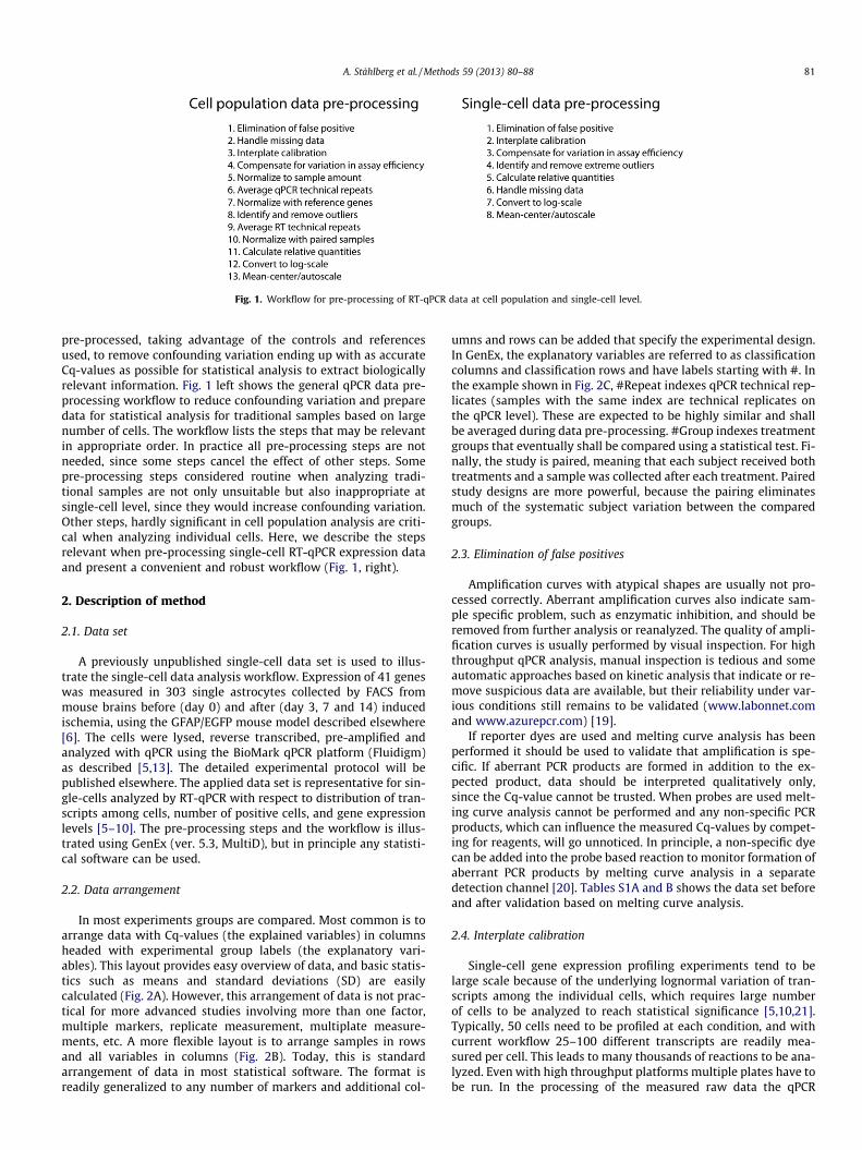
Fig. 1. Workflow for pre-processing of RT-qPCR data at cell population and single-cell level.

A. Ståhlberg et al. / Methods 59 (2013) 80–88 81

pre-processed, taking advantage of the controls and referencesused, to remove confounding variation ending up with as accurateCq-values as possible for statistical analysis to extract biologicallyrelevant information. Fig. 1 left shows the general qPCR data pre-processing workflow to reduce confounding variation and preparedata for statistical analysis for traditional samples based on largenumber of cells. The workflow lists the steps that may be relevantin appropriate order. In practice all pre-processing steps are notneeded, since some steps cancel the effect of other steps. Somepre-processing steps considered routine when analyzing tradi-tional samples are not only unsuitable but also inappropriate atsingle-cell level, since they would increase confounding variation.Other steps, hardly significant in cell population analysis are criti-cal when analyzing individual cells. Here, we describe the stepsrelevant when pre-processing single-cell RT-qPCR expression dataand present a convenient and robust workflow (Fig. 1, right).

2. Description of method

2.1. Data set

A previously unpublished single-cell data set is used to illus-trate the single-cell data analysis workflow. Expression of 41 geneswas measured in 303 single astrocytes collected by FACS frommouse brains before (day 0) and after (day 3, 7 and 14) inducedischemia, using the GFAP/EGFP mouse model described elsewhere[6]. The cells were lysed, reverse transcribed, pre-amplified andanalyzed with qPCR using the BioMark qPCR platform (Fluidigm)as described [5,13]. The detailed experimental protocol will bepublished elsewhere. The applied data set is representative for sin-gle-cells analyzed by RT-qPCR with respect to distribution of tran-scripts among cells, number of positive cells, and gene expressionlevels [5–10]. The pre-processing steps and the workflow is illus-trated using GenEx (ver. 5.3, MultiD), but in principle any statisti-cal software can be used.

2.2. Data arrangement

In most experiments groups are compared. Most common is toarrange data with Cq-values (the explained variables) in columnsheaded with experimental group labels (the explanatory vari-ables). This layout provides easy overview of data, and basic statis-tics such as means and standard deviations (SD) are easilycalculated (Fig. 2A). However, this arrangement of data is not prac-tical for more advanced studies involving more than one factor,multiple markers, replicate measurement, multiplate measure-ments, etc. A more flexible layout is to arrange samples in rowsand all variables in columns (Fig. 2B). Today, this is standardarrangement of data in most statistical software. The format isreadily generalized to any number of markers and additional col-

umns and rows can be added that specify the experimental design.In GenEx, the explanatory variables are referred to as classificationcolumns and classification rows and have labels starting with #. Inthe example shown in Fig. 2C, #Repeat indexes qPCR technical rep-licates (samples with the same index are technical replicates onthe qPCR level). These are expected to be highly similar and shallbe averaged during data pre-processing. #Group indexes treatmentgroups that eventually shall be compared using a statistical test. Fi-nally, the study is paired, meaning that each subject received bothtreatments and a sample was collected after each treatment. Pairedstudy designs are more powerful, because the pairing eliminatesmuch of the systematic subject variation between the comparedgroups.

2.3. Elimination of false positives

Amplification curves with atypical shapes are usually not pro-cessed correctly. Aberrant amplification curves also indicate sam-ple specific problem, such as enzymatic inhibition, and should beremoved from further analysis or reanalyzed. The quality of ampli-fication curves is usually performed by visual inspection. For highthroughput qPCR analysis, manual inspection is tedious and someautomatic approaches based on kinetic analysis that indicate or re-move suspicious data are available, but their reliability under var-ious conditions still remains to be validated (www.labonnet.comand www.azurepcr.com) [19].

If reporter dyes are used and melting curve analysis has beenperformed it should be used to validate that amplification is spe-cific. If aberrant PCR products are formed in addition to the ex-pected product, data should be interpreted qualitatively only,since the Cq-value cannot be trusted. When probes are used melt-ing curve analysis cannot be performed and any non-specific PCRproducts, which can influence the measured Cq-values by compet-ing for reagents, will go unnoticed. In principle, a non-specific dyecan be added into the probe based reaction to monitor formation ofaberrant PCR products by melting curve analysis in a separatedetection channel [20]. Tables S1A and B shows the data set beforeand after validation based on melting curve analysis.

2.4. Interplate calibration

Single-cell gene expression profiling experiments tend to belarge scale because of the underlying lognormal variation of tran-scripts among the individual cells, which requires large numberof cells to be analyzed to reach statistical significance [5,10,21].Typically, 50 cells need to be profiled at each condition, and withcurrent workflow 25–100 different transcripts are readily mea-sured per cell. This leads to many thousands of reactions to be ana-lyzed. Even with high throughput platforms multiple plates have tobe run. In the processing of the measured raw data the qPCR

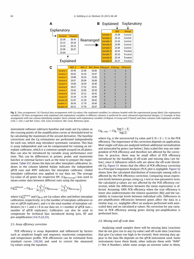
Fig. 2. Data arrangement. (A) Classical data arrangement with Cq-values (the explained variables) in columns headed with the experimental group labels (the explanatoryvariables). (B) Data arrangement with explained and explanatory variables in different columns is preferred for more advanced experimental designs. (C) Example of dataarrangement with one column identifying samples, three columns with explanatory variables (# Repeat, # Group and # Paired) and three columns with explained variables(GOI_1, GOI_2 and Ref. Gene). GOI, Gene of interest; Ref. Gene, Reference gene.

82 A. Ståhlberg et al. / Methods 59 (2013) 80–88

instrument software subtracts baseline and reads out Cq-values asthe crossing points of the amplification curves at threshold level orby calculating the maximum of the second derivative. The baselinecorrections and the Cq estimations are performed independentlyfor each run, which may introduce systematic variation. This biasis assay independent and can be compensated for running an int-erplate calibrator, which is a common sample assayed on all plates.Bias can also be introduced by variable assay performance overtime. This can be differences in primer, probe, and mastermixbatches or external factors such as the time to prepare the exper-iment. Table S1C shows the data set after interplate calibration. In-dexes in the column labeled #plate indicates the independentqPCR runs and #IPC indicates the interplate calibrator. Globalinterplate calibration was applied to our data set. The averageCq-value of all genes for respective IPC (CqIPCAverage) was used tomean-center data between different runs using the equation:

CqCalibtratedGOI ¼ CqGOI �

1m

Xm

j¼1

CqIPCAverage �1n

Xn

i¼1

CqIPCAverage

!

where CqCalibratedGOI and CqGOI are Cq-values after and before interplate

calibration, respectively. m is the number of interplate calibrators inrun m (qPCR replicates), and n is the total number of interplate cal-ibrators (m = 1 and n = 8 in our data set, n = number of qPCR runs ⁄number of qPCR replicates). Calibrators can also be used tocompensate for technical bias introduced during lysis, RT andpre-amplification [14,15,22,23].

2.5. Assay efficiency correction

PCR efficiency is assay dependent and influenced by factorssuch as amplicon length and sequence, mastermix composition,and temperature profile. PCR efficiencies can be estimated fromstandard curves [18,24] and used to correct the measuredCq-values using the equation:

CqE¼100% ¼ CqElogð1þ EÞ

logð2Þ

where CqE is the uncorrected Cq value and E (0 6 E 6 1) is the PCRefficiency. The importance of the correction depends on application.Most single-cell data are analyzed without additional normalizationand autoscaled by genes (see below). Data scaled this way are inde-pendent of PCR efficiency and therefore not affected by the correc-tion. In practice, there may be small effect of PCR efficiencyintroduced by the handling of off-scale and missing data (see be-low), since it influences which cells are above the off-scale thresh-old Cq. Figure S1 shows that the effect of PCR efficiency correctionin a Principal Component Analysis (PCA) plot is negligible. Figure S2shows how the calculated distribution of transcripts among cells isaffected by the PCR efficiency correction. Comparing mean expres-sion levels between groups, using e.g. t-test or non-parametric tests,the calculated p-values are not affected by the PCR efficiency cor-rection, while the difference between the mean expressions is af-fected. Assuming 100% PCR efficiency when the true efficiency islower also underestimates the relative quantities (RQ) and the var-iability in transcript levels between individual cells. Differences inpre-amplification efficiencies between genes affect the data in asimilar way, i.e., negligible effect on analyses performed with auto-scaled data and on calculated p-values. No correction for any varia-tion in PCR efficiency among genes during pre-amplification isperformed here.

2.6. Missing and off scale data

Analyzing small samples there will be missing data (reactionsthat do not give rise to any Cq-value) and off-scale data (reactionsthat give Cq-values too high to be trusted). How missing data ap-pear in the data file depends on the qPCR instrument used. Someinstruments leave them blank, other indicate them with ‘‘NAN’’(= Not A Number), while some assign an extreme value to them,

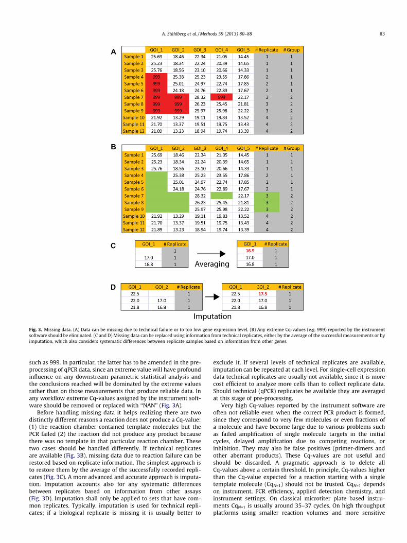
Fig. 3. Missing data. (A) Data can be missing due to technical failure or to too low gene expression level. (B) Any extreme Cq-values (e.g. 999) reported by the instrumentsoftware should be eliminated. (C and D) Missing data can be replaced using information from technical replicates, either by the average of the successful measurements or byimputation, which also considers systematic differences between replicate samples based on information from other genes.

A. Ståhlberg et al. / Methods 59 (2013) 80–88 83

such as 999. In particular, the latter has to be amended in the pre-processing of qPCR data, since an extreme value will have profoundinfluence on any downstream parametric statistical analysis andthe conclusions reached will be dominated by the extreme valuesrather than on those measurements that produce reliable data. Inany workflow extreme Cq-values assigned by the instrument soft-ware should be removed or replaced with ‘‘NAN’’ (Fig. 3A).

Before handling missing data it helps realizing there are twodistinctly different reasons a reaction does not produce a Cq-value:(1) the reaction chamber contained template molecules but thePCR failed (2) the reaction did not produce any product becausethere was no template in that particular reaction chamber. Thesetwo cases should be handled differently. If technical replicatesare available (Fig. 3B), missing data due to reaction failure can berestored based on replicate information. The simplest approach isto restore them by the average of the successfully recorded repli-cates (Fig. 3C). A more advanced and accurate approach is imputa-tion. Imputation accounts also for any systematic differencesbetween replicates based on information from other assays(Fig. 3D). Imputation shall only be applied to sets that have com-mon replicates. Typically, imputation is used for technical repli-cates; if a biological replicate is missing it is usually better to

exclude it. If several levels of technical replicates are available,imputation can be repeated at each level. For single-cell expressiondata technical replicates are usually not available, since it is morecost efficient to analyze more cells than to collect replicate data.Should technical (qPCR) replicates be available they are averagedat this stage of pre-processing.

Very high Cq-values reported by the instrument software areoften not reliable even when the correct PCR product is formed,since they correspond to very few molecules or even fractions ofa molecule and have become large due to various problems suchas failed amplification of single molecule targets in the initialcycles, delayed amplification due to competing reactions, orinhibition. They may also be false positives (primer-dimers andother aberrant products). These Cq-values are not useful andshould be discarded. A pragmatic approach is to delete allCq-values above a certain threshold. In principle, Cq-values higherthan the Cq-value expected for a reaction starting with a singletemplate molecule (CqN=1) should not be trusted. CqN=1 dependson instrument, PCR efficiency, applied detection chemistry, andinstrument settings. On classical microtiter plate based instru-ments CqN=1 is usually around 35–37 cycles. On high throughputplatforms using smaller reaction volumes and more sensitive

84 A. Ståhlberg et al. / Methods 59 (2013) 80–88

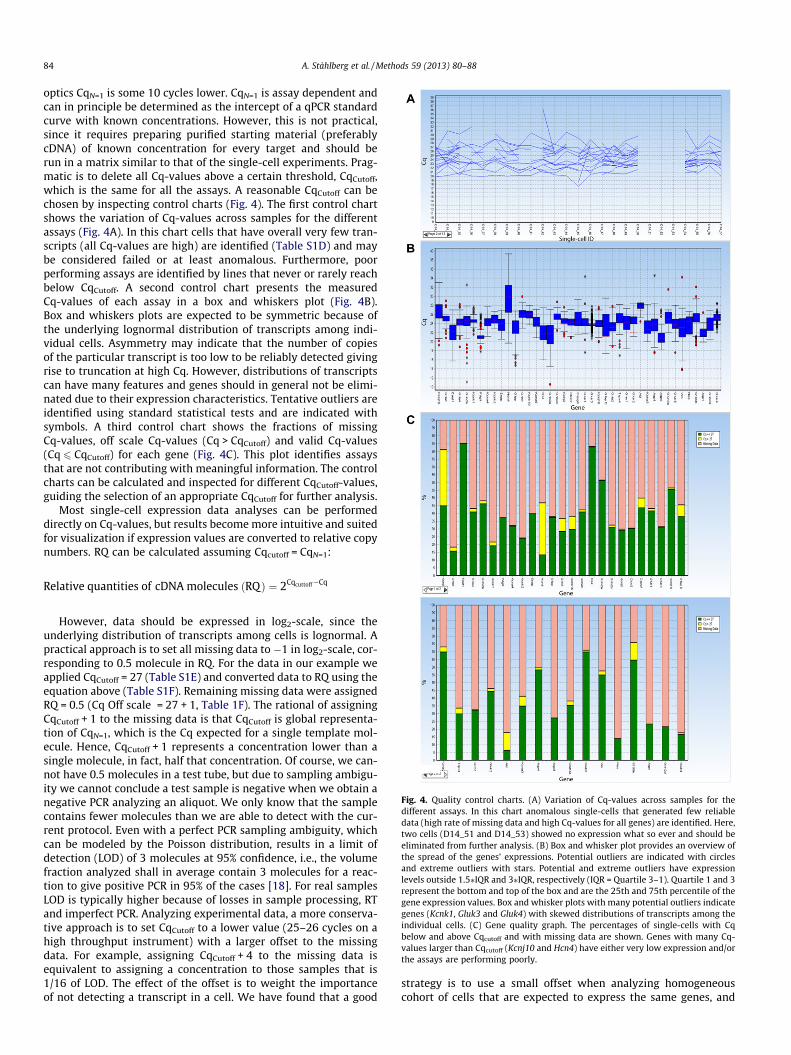
optics CqN=1 is some 10 cycles lower. CqN=1 is assay dependent andcan in principle be determined as the intercept of a qPCR standardcurve with known concentrations. However, this is not practical,since it requires preparing purified starting material (preferablycDNA) of known concentration for every target and should berun in a matrix similar to that of the single-cell experiments. Prag-matic is to delete all Cq-values above a certain threshold, CqCutoff,which is the same for all the assays. A reasonable CqCutoff can bechosen by inspecting control charts (Fig. 4). The first control chartshows the variation of Cq-values across samples for the differentassays (Fig. 4A). In this chart cells that have overall very few tran-scripts (all Cq-values are high) are identified (Table S1D) and maybe considered failed or at least anomalous. Furthermore, poorperforming assays are identified by lines that never or rarely reachbelow CqCutoff. A second control chart presents the measuredCq-values of each assay in a box and whiskers plot (Fig. 4B).Box and whiskers plots are expected to be symmetric because ofthe underlying lognormal distribution of transcripts among indi-vidual cells. Asymmetry may indicate that the number of copiesof the particular transcript is too low to be reliably detected givingrise to truncation at high Cq. However, distributions of transcriptscan have many features and genes should in general not be elimi-nated due to their expression characteristics. Tentative outliers areidentified using standard statistical tests and are indicated withsymbols. A third control chart shows the fractions of missingCq-values, off scale Cq-values (Cq > CqCutoff) and valid Cq-values(Cq 6 CqCutoff) for each gene (Fig. 4C). This plot identifies assaysthat are not contributing with meaningful information. The controlcharts can be calculated and inspected for different CqCutoff-values,guiding the selection of an appropriate CqCutoff for further analysis.

Most single-cell expression data analyses can be performeddirectly on Cq-values, but results become more intuitive and suitedfor visualization if expression values are converted to relative copynumbers. RQ can be calculated assuming Cqcutoff = CqN=1:

Fig. 4. Quality control charts. (A) Variation of Cq-values across samples for thedifferent assays. In this chart anomalous single-cells that generated few reliabledata (high rate of missing data and high Cq-values for all genes) are identified. Here,two cells (D14_51 and D14_53) showed no expression what so ever and should beeliminated from further analysis. (B) Box and whisker plot provides an overview ofthe spread of the genes’ expressions. Potential outliers are indicated with circlesand extreme outliers with stars. Potential and extreme outliers have expressionlevels outside 1.5⁄IQR and 3⁄IQR, respectively (IQR = Quartile 3–1). Quartile 1 and 3represent the bottom and top of the box and are the 25th and 75th percentile of thegene expression values. Box and whisker plots with many potential outliers indicategenes (Kcnk1, Gluk3 and Gluk4) with skewed distributions of transcripts among theindividual cells. (C) Gene quality graph. The percentages of single-cells with Cqbelow and above Cqcutoff and with missing data are shown. Genes with many Cq-values larger than Cqcutoff (Kcnj10 and Hcn4) have either very low expression and/orthe assays are performing poorly.

Relative quantities of cDNA molecules ðRQÞ ¼ 2Cqcuttoff�Cq

However, data should be expressed in log2-scale, since theunderlying distribution of transcripts among cells is lognormal. Apractical approach is to set all missing data to �1 in log2-scale, cor-responding to 0.5 molecule in RQ. For the data in our example weapplied CqCutoff = 27 (Table S1E) and converted data to RQ using theequation above (Table S1F). Remaining missing data were assignedRQ = 0.5 (Cq Off scale = 27 + 1, Table 1F). The rational of assigningCqCutoff + 1 to the missing data is that CqCutoff is global representa-tion of CqN=1, which is the Cq expected for a single template mol-ecule. Hence, CqCutoff + 1 represents a concentration lower than asingle molecule, in fact, half that concentration. Of course, we can-not have 0.5 molecules in a test tube, but due to sampling ambigu-ity we cannot conclude a test sample is negative when we obtain anegative PCR analyzing an aliquot. We only know that the samplecontains fewer molecules than we are able to detect with the cur-rent protocol. Even with a perfect PCR sampling ambiguity, whichcan be modeled by the Poisson distribution, results in a limit ofdetection (LOD) of 3 molecules at 95% confidence, i.e., the volumefraction analyzed shall in average contain 3 molecules for a reac-tion to give positive PCR in 95% of the cases [18]. For real samplesLOD is typically higher because of losses in sample processing, RTand imperfect PCR. Analyzing experimental data, a more conserva-tive approach is to set CqCutoff to a lower value (25–26 cycles on ahigh throughput instrument) with a larger offset to the missingdata. For example, assigning CqCutoff + 4 to the missing data isequivalent to assigning a concentration to those samples that is1/16 of LOD. The effect of the offset is to weight the importanceof not detecting a transcript in a cell. We have found that a good

strategy is to use a small offset when analyzing homogeneouscohort of cells that are expected to express the same genes, and

A. Ståhlberg et al. / Methods 59 (2013) 80–88 85

a large offset when objective is to distinguish between cell typesthat exclusively express some markers. Figure S3 shows the effectof changing Cqcutoff = 27 to Cqcutoff = 25 on PCA, and Figure S4shows the effect of offset when assigning different Cq-values tothe missing data. For this particular data set the CqCutoff-valueand the offset have insignificant effect on the analysis result. Thisis usually the case. Still, we recommend users to test the effectsof CqCutoff and offset when analyzing new data to validate therobustness of their handling of missing data. One should also becautious when key classification genes are expressed at low levelwith high Cq-values. It is then important to set CqCutoff at a valuethat distinguishes between positive and negative cells with respectto this marker. In some cases it may be necessary to treat key clas-sifiers separately, using an assay specific Cqcutoff. Genes that may bebiased due to the choice of Cqcutoff are identified in the controlcharts (Figs. 4B and C). The rationale of handling missing data after,instead of before, the transformation to RQ is that RQ of the Cqcut-

off-value (and not of Cqcutoff + 1) shall be assigned arbitrary expres-sion of 1 (zero in log2-scale). The RQs after handling missing dataand RQs in log2-scale are shown in Tables S1G and S1H, respec-tively. Conversion of relative quantities to the number of cDNAmolecules or to the number of mRNA molecules requires calibra-tion with standards [9,14,25]. Missing data due to few target mol-ecules in the reaction vessel is in single-cell studies with goodassays more common than reaction failure. Missing data can there-fore be replaced with Cqcutoff + offset instead of imputation or aver-aging even when qPCR replicates are available. In practice the twooptions to handle missing data will produce very similar results.

2.7. Basic statistics and distributions

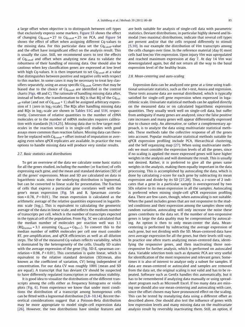
To get an overview of the data we calculate some basic staticsfor all the genes studied, including the number (or fraction) of cellsexpressing each gene, and the mean and standard deviation (SD) ofall the genes’ expressions. Mean and SD are calculated on data inlogarithmic scale, since the underlying distribution is lognormal,but can be converted to linear scale for presentation. The fractionof cells that express a particular gene correlates well with thegene’s mean expression (Fig. 5A and B, Spearman correla-tion = 0.78, P < 0.01). The mean expression is calculated as thearithmetic average of the relative quantities expressed in logarith-mic scale (log2). This is equivalent to calculating the geometricaverage of the data in linear scale, and reflects the medium numberof transcripts per cell, which is the number of transcripts expectedin the typical cell of the population. From Fig. 5C we calculated thatthe median number of molecules per reaction well was 3.1(RQmedian = 3.1 assuming Cqcutoff = CqN=1). To convert this to themedian number of mRNA molecules per cell one must considerRT, pre-amplification, and qPCR efficiencies as well as all dilutionsteps. The SD of the measured Cq-values reflects variability, whichis dominated by the heterogeneity of the cells. Usually SD scaleswith the average expression of the gene (Fig. 5D-E, spearman cor-relation = 0.98, P < 0.01). This correlation is quite linear, which isequivalent to the relative standard deviation (SD/mean, alsoknown as the coefficient of variation, CV) being independent ofconcentration. For our data CV was roughly 100% (mean and SDare equal). A transcript that has deviant CV should be suspectedto have differently regulated transcription or anomalous stability.

It is good idea to visualize the distributions of the different tran-scripts among the cells either as frequency histograms or violinplots (Fig. 6). From experience we know that under most condi-tions the distribution of a transcript among homogenous cellscan be fitted with a lognormal distribution [5,8–10,14]. Recent the-oretical considerations suggest that a Poisson-Beta distributionmay be more appropriate to model single-cell expression data[26]. However, the two distributions have similar features and

are both suitable for analysis of single-cell data with parametricstatistics. Deviant distributions, in particular highly skewed and bi-modal (two maxima) distributions, indicate that several cell typesare present and/or that the cells respond differently to stimuli[5,10]. In our example the distribution of Vim transcripts amongthe cells changes over time. In the reference material (day 0) mostcells had low/no Vim expression. Upon injury Vim was upregulatedand reached maximum expression at day 7. At day 14 Vim wasdownregulated again, but did not return all the way to the basalexpression level of the healthy brain.

2.8. Mean-centering and auto-scaling

Expression data can be analyzed one gene at a time using tradi-tional univariate statistics, such as the t-test, Anova and regression.These tests assume data are normal distributed, which is typicallysatisfied for single-cell gene expression when expressed in loga-rithmic scale. Univariate statistical methods can be applied directlyon the measured data or on calculated logarithmic expressionquantities. They usually work well on single-cell data, but sufferfrom ambiguity if many genes are analyzed, since the false positiverate increases and many genes will appear differentially expresseddue to chance only. An alternative, or rather a complementary ap-proach, is to analyze the data using multivariate statistical meth-ods. These methods take the collective response of all the genesinto account. Popular multivariate statistical methods suitable forqPCR expression profiling include PCA, Hierarchical clustering,and the Self organizing map [27]. When using multivariate meth-ods we must consider the expression levels of all the genes, sinceif no scaling is applied the more expressed genes will have higherweights in the analysis and will dominate the result. This is usuallynot desired. Rather, it is preferred to give all the genes sameweights in the analysis, making them equally important in the dataprocessing. This is accomplished by autoscaling the data, which isdone by calculating z-score for each gene by subtracting its meanexpression and divide by its SD [27,28]. Thus, a z-score of 2 indi-cates that a gene in a particular sample is overexpressed by twoSDs relative to its mean expression in all the samples. Autoscalingis preferred when mining single-cell qPCR expression profilingdata. There are few cases, though, when autoscaling is not suitable.When the panel includes genes that are not responsive to the stud-ied conditions and their expression among the samples show onlyrandom variation, autoscaling will only increase the noise thesegenes contribute to the data set. If the number of non-responsivegenes is large the data quality may be compromised by autoscal-ing. An option is then to only mean-center the data. Mean-centering is performed by subtracting the average expression ofeach gene, but not dividing with the SD. Mean-centered data havezero average expression for all the genes, but their levels still vary.In practice one often starts analyzing mean-centered data, identi-fying the responsive genes, and then inactivating those non-responsive for further analysis, which is performed on autoscaleddata. Variable selection tools such as dynamic PCA are very usefulfor identification of the most responsive and relevant genes. Some-times it is also of interest to analyze only a subset for samples. Ifdata are mean-centered or autoscaled and samples are removedfrom the data set, the original scaling is not valid and has to be re-peated. Software such as GenEx handles this automatically, but ithas to be remembered if analyzing data manually or using spread-sheet program such as Microsoft Excel. If too many data are miss-ing one should also use mean-centering and autoscaling with care,since the offset chosen may have pronounced effect on the scaling.This can be tested by reanalyzing data using a different offset asdescribed above. One should also test the influence of genes withlow expression levels and many missing data on the multivariateanalysis result by reversibly inactivating them. Still, an option, if

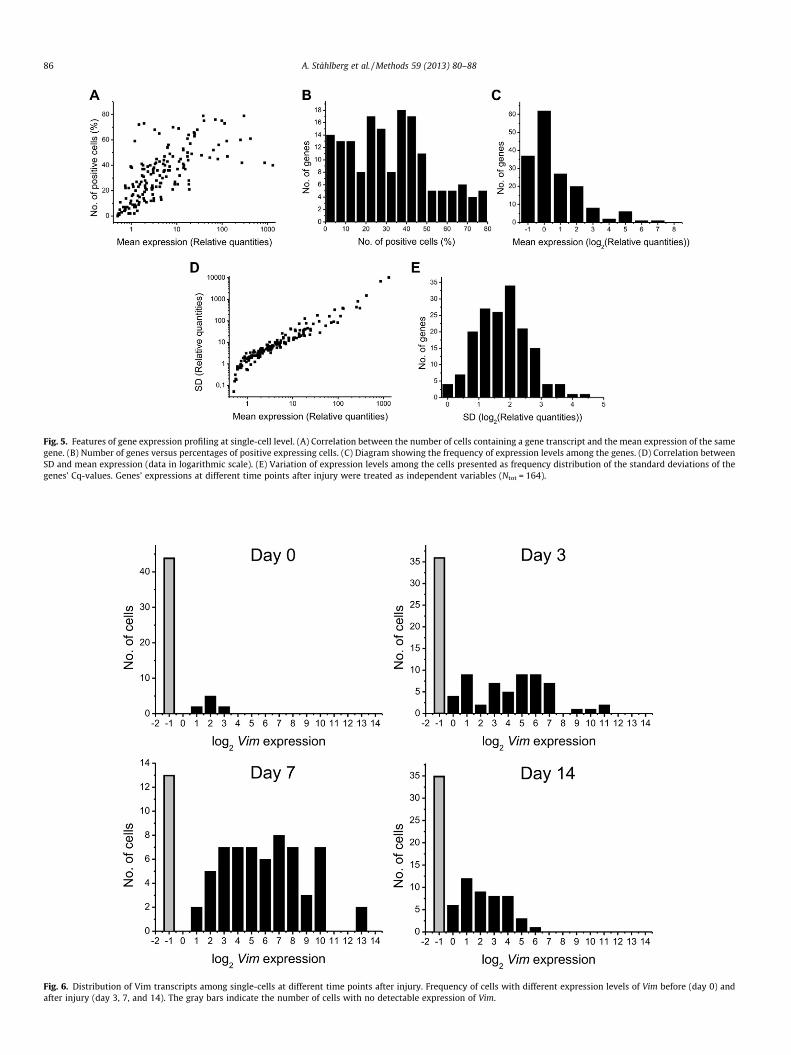
Fig. 5. Features of gene expression profiling at single-cell level. (A) Correlation between the number of cells containing a gene transcript and the mean expression of the samegene. (B) Number of genes versus percentages of positive expressing cells. (C) Diagram showing the frequency of expression levels among the genes. (D) Correlation betweenSD and mean expression (data in logarithmic scale). (E) Variation of expression levels among the cells presented as frequency distribution of the standard deviations of thegenes’ Cq-values. Genes’ expressions at different time points after injury were treated as independent variables (Ntot = 164).

Fig. 6. Distribution of Vim transcripts among single-cells at different time points after injury. Frequency of cells with different expression levels of Vim before (day 0) andafter injury (day 3, 7, and 14). The gray bars indicate the number of cells with no detectable expression of Vim.

86 A. Ståhlberg et al. / Methods 59 (2013) 80–88

A. Ståhlberg et al. / Methods 59 (2013) 80–88 87

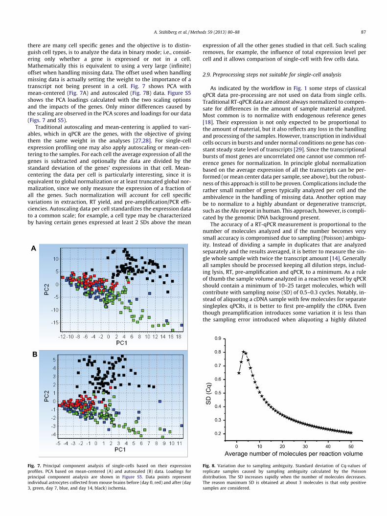
there are many cell specific genes and the objective is to distin-guish cell types, is to analyze the data in binary mode; i.e., consid-ering only whether a gene is expressed or not in a cell.Mathematically this is equivalent to using a very large (infinite)offset when handling missing data. The offset used when handlingmissing data is actually setting the weight to the importance of atranscript not being present in a cell. Fig. 7 shows PCA withmean-centered (Fig. 7A) and autoscaled (Fig. 7B) data. Figure S5shows the PCA loadings calculated with the two scaling optionsand the impacts of the genes. Only minor differences caused bythe scaling are observed in the PCA scores and loadings for our data(Figs. 7 and S5).

Traditional autoscaling and mean-centering is applied to vari-ables, which in qPCR are the genes, with the objective of givingthem the same weight in the analyses [27,28]. For single-cellexpression profiling one may also apply autoscaling or mean-cen-tering to the samples. For each cell the average expression of all thegenes is subtracted and optionally the data are divided by thestandard deviation of the genes’ expressions in that cell. Mean-centering the data per cell is particularly interesting, since it isequivalent to global normalization or at least truncated global nor-malization, since we only measure the expression of a fraction ofall the genes. Such normalization will account for cell specificvariations in extraction, RT yield, and pre-amplification/PCR effi-ciencies. Autoscaling data per cell standardizes the expression datato a common scale; for example, a cell type may be characterizedby having certain genes expressed at least 2 SDs above the mean

Fig. 7. Principal component analysis of single-cells based on their expressionprofiles. PCA based on mean-centered (A) and autoscaled (B) data. Loadings forprincipal component analysis are shown in Figure S5. Data points representindividual astrocytes collected from mouse brains before (day 0, red) and after (day3, green, day 7, blue, and day 14, black) ischemia.

expression of all the other genes studied in that cell. Such scalingremoves, for example, the influence of total expression level percell and it allows comparison of single-cell with few cells data.

2.9. Preprocessing steps not suitable for single-cell analysis

As indicated by the workflow in Fig. 1 some steps of classicalqPCR data pre-processing are not used on data from single cells.Traditional RT-qPCR data are almost always normalized to compen-sate for differences in the amount of sample material analyzed.Most common is to normalize with endogenous reference genes[18]. Their expression is not only expected to be proportional tothe amount of material, but it also reflects any loss in the handlingand processing of the samples. However, transcription in individualcells occurs in bursts and under normal conditions no gene has con-stant steady state level of transcripts [29]. Since the transcriptionalbursts of most genes are uncorrelated one cannot use common ref-erence genes for normalization. In principle global normalizationbased on the average expression of all the transcripts can be per-formed (or mean center data per sample, see above), but the robust-ness of this approach is still to be proven. Complications include therather small number of genes typically analyzed per cell and theambivalence in the handling of missing data. Another option maybe to normalize to a highly abundant or degenerative transcript,such as the Alu repeat in human. This approach, however, is compli-cated by the genomic DNA background present.

The accuracy of a RT-qPCR measurement is proportional to thenumber of molecules analyzed and if the number becomes verysmall accuracy is compromised due to sampling (Poisson) ambigu-ity. Instead of dividing a sample in duplicates that are analyzedseparately and the results averaged, it is better to measure the sin-gle whole sample with twice the transcript amount [14]. Generallyall samples should be processed keeping all dilution steps, includ-ing lysis, RT, pre-amplification and qPCR, to a minimum. As a ruleof thumb the sample volume analyzed in a reaction vessel by qPCRshould contain a minimum of 10–25 target molecules, which willcontribute with sampling noise (SD) of 0.5–0.3 cycles. Notably, in-stead of aliquoting a cDNA sample with few molecules for separatesingleplex qPCRs, it is better to first pre-amplify the cDNA. Eventhough preamplification introduces some variation it is less thanthe sampling error introduced when aliquoting a highly diluted

Fig. 8. Variation due to sampling ambiguity. Standard deviation of Cq-values ofreplicate samples caused by sampling ambiguity calculated by the Poissondistribution. The SD increases rapidly when the number of molecules decreases.The reason maximum SD is obtained at about 3 molecules is that only positivesamples are considered.

88 A. Ståhlberg et al. / Methods 59 (2013) 80–88

sample (Fig. 8) and [15,22,23]. After pre-amplification the amountof transcripts is usually high enough to allow technical qPCR repli-cates to be measured, as a reassurance if a qPCR fails. From a cost-performance and statistical perspective, though, it is usually betterto analyze larger number of single-cells than performing technicalreplicates. Of course, in the validation of assays, including controls,standard curves and LOD, technical replicates should be measured[18].

2.10. Classification algorithms

Analysis of data and data mining is usually hypothesis drivenand therefore application dependent and the different methodsavailable have been discussed elsewhere [5,27,28]. Here we onlyuse PCA to visualize some of the important features of the pre-processing using an example data set collected on astrocytesharvested at different time points after brain injury in mice. PCAclearly reveals changes in gene expression profiles at the single-cell level occurring over time, reflecting heterogeneity and celltransformation induced by the injury. Other powerful methods toanalyze and classify individual cells include hierarchical clustering,and the self organizing map [5,27,28].

3. Concluding remarks

Gene expression profiling using RT-qPCR took a major leap for-ward by the publication of the MIQE guidelines, which help usersanalyzing classical samples [18]. For single-cell profiling some as-pects (e.g., reference gene normalization) of the standard workfloware not valid or applicable, while other options (e.g., mean-centering and autoscaling along samples) are almost compulsory.Here we present a complete workflow for the pre-processing ofsingle-cell RT-qPCR data that is robust and prepares the data in ameaningful way for further analysis and mining. Using an exampledata set we also present several characteristics of single-cellexpression data. For some pre-processing steps we present optionsand also recommendations based on the experience gathered sofar. The aim of this workflow is to provide guidelines to the rapidlygrowing community studying single-cells by means of RT-qPCRprofiling. To further stimulate exchange and experiences in thesingle-cell expression field we have made our example dataavailable in supplement.

4. Disclosure

A.S., V.R., A.F. and M.K. declare stock ownership in TATAA Bio-center AB. A.F. and M.K. also declare stock ownership in MultiD.

Acknowledgements

This work was partly supported by grants from AssarGabrielssons Research Foundation, Johan Jansson Foundation forCancer Research, Socialstyrelsen, Swedish Society for MedicalResearch, The Swedish Research Council (A.S. 521-2011-2367),

EMBO Short Term Fellowship (V.R.), ESF Functional Genomics ShortVisit Grant (A.S. and V.R.), BioCARE National Strategic ResearchProgram at University of Gothenburg, Wilhelm and Martina Lund-gren Foundation for Scientific Research, the grant of Czech Ministryof Education ME10052, the research project AV0Z50520701, andGACR GA P303/10/1338.

Appendix A. Supplementary data

Supplementary data associated with this article can be found, inthe online version, at http://dx.doi.org/10.1016/j.ymeth.2012.09.007.

References

[1] T. Kalisky, P. Blainey, S.R. Quake, Annu. Rev. Genet. 45 (2011) 431–435.[2] M. Wu, A.K. Singh, Curr. Opin. Biotechnol. 23 (2012) 83–88.[3] D.R. Larson, R.H. Singer, D. Zenklusen, Trends Cell Biol. 19 (2009) 630–637.[4] B. Liss, O. Franz, S. Sewing, R. Bruns, H. Neuhoff, J. Roeper, EMBO J. 20 (2001)

5715–5724.[5] A. Ståhlberg, D. Andersson, J. Aurelius, M. Faiz, M. Pekna, M. Kubista, M. Pekny,

Nucleic Acids Res. 39 (2011) e24.[6] J. Benesova, V. Rusnakova, P. Honsa, H. Pivonkova, D. Dzamba, M. Kubista, M.

Anderova, PLoS One 7 (2012) e29725.[7] A. Ståhlberg, M. Bengtsson, M. Hemberg, H. Semb, Clin. Chem. 55 (2009) 2162–

2170.[8] K.H. Narsinh, N. Sun, V. Sanchez-Freire, A.S. Lee, P. Almeida, S. Hu, T. Jan, K.D.

Wilson, D. Leong, J. Rosenberg, et al., J. Clin. Invest. 121 (2011) 1217–1221.[9] K. Norrman, A. Strömbeck, H. Semb, A. Ståhlberg, Distinct gene expression

signatures in human embryonic stem cells differentiated towards definitiveendoderm at single-cell level, Methods 59 (2012) 59–70.

[10] M. Bengtsson, A. Ståhlberg, P. Rorsman, M. Kubista, Genome Res. 15 (2005)1388–1392.

[11] F. Kamme, R. Salunga, J. Yu, D.T. Tran, J. Zhu, L. Luo, A. Bittner, H.Q. Guo, N.Miller, J. Wan, et al., J. Neurosci. 23 (2003) 3607–3615.

[12] J. Gründemann, F. Schlaudraff, O. Haeckel, B. Liss, Nucleic Acids Res. 36 (2008)e38.

[13] A. Ståhlberg, M. Bengtsson, Methods 50 (2010) 282–288.[14] M. Bengtsson, M. Hemberg, P. Rorsman, A. Ståhlberg, BMC Mol. Biol. 9 (2008)

63.[15] B.C. Fox, A.S. Devonshire, M.O. Baradez, D. Marshall, C.A. Foy, Anal. Biochem.

472 (2012) 178–186.[16] P. Dalerba, T. Kalisky, D. Sahoo, P.S. Rajendran, M.E. Rothenberg, A.A. Leyrat, S.

Sim, J. Okamoto, D.M. Johnston, D. Qian, et al., Nat. Biotechnol. 29 (2011)1120–1127.

[17] G. Guo, M. Huss, G.Q. Tong, C. Wang, L. Li Sun, N.D. Clarke, P. Robson, Dev. Cell18 (2010) 675–685.

[18] S.A. Bustin, V. Benes, J.A. Garson, J. Hellemans, J. Huggett, M. Kubista, R.Mueller, T. Nolan, M.W. Pfaffl, G.L. Shipley, J. Vandesompele, C.T. Wittwer, Clin.Chem. 55 (2009) 611–622.

[19] T. Bar, M. Kubista, A. Tichopad, Nucleic Acids Res. 40 (2012) 1395–1406.[20] K. Lind, A. Ståhlberg, N. Zoric, M. Kubista, Biotechniques 40 (2006) 315–319.[21] A. Ståhlberg, M. Kubista, P. Åman, Expert Rev. Mol. Diagn. 11 (2011) 735–740.[22] A.S. Devonshire, R. Elaswarapu, C.A. Foy, BMC Geomics 12 (2011) 118.[23] M. Reiter, B. Kirchner, H. Müller, C. Holzhauer, W. Mann, M.W. Pfaffl, Nucleic

Acids Res. 39 (2011) e124.[24] A. Ståhlberg, P. Åman, B. Ridell, P. Mostad, M. Kubista, Clin. Chem. 49 (2003)

51–59.[25] A. Ståhlberg, M. Kubista, M. Pfaffl, Clin. Chem. 50 (2004) 1678–1680.[26] A. Raj, C.S. Peskin, D. Tranchina, D.Y. Vargas, S. Tyagi, PLoS Biol. 4 (2006) e309.[27] A. Bergkvist, V. Rusnakova, R. Sindelka, J.M. Garda, B. Sjögreen, D. Lindh, A.

Forootan, M. Kubista, Methods 50 (2010) 323–335.[28] A. Ståhlberg, K. Elbing, J. Andrade-Garda, B. Sjögreen, A. Forootan, M. Kubista,

BMC Genomics 9 (2008) 170.[29] A. Raj, A. van Oudenaarden, Cell 135 (2008) 216–226.