Embed Size (px)
Citation preview
3434 IEEE ROBOTICS AND AUTOMATION LETTERS, VOL. 3, NO. 4, OCTOBER 2018
RT3D: Real-Time 3-D Vehicle Detection in LiDARPoint Cloud for Autonomous Driving
Yiming Zeng , Yu Hu , Shice Liu , Jing Ye , Yinhe Han , Xiaowei Li , and Ninghui Sun
Abstract—For autonomous driving, vehicle detection is the pre-requisite for many tasks like collision avoidance and path planning.In this letter, we present a real-time three-dimensional (RT3D) ve-hicle detection method that utilizes pure LiDAR point cloud topredict the location, orientation, and size of vehicles. In contrast toprevious 3-D object detection methods, we used a pre-RoIpoolingconvolution technique that moves a majority of the convolutionoperations to ahead of the RoI pooling, leaving just a small partbehind, so that significantly boosts the computation efficiency. Wealso propose a pose-sensitive feature map design which can bestrongly activated by the relative poses of vehicles, leading to ahigh regression accuracy on the location, orientation, and size ofvehicles. Experiments on the KITTI benchmark dataset show thatthe RT3D is not only able to deliver competitive detection accuracyagainst state-of-the-art methods, but also the first LiDAR-based3-D vehicle detection work that completes detection within 0.09 swhich is even shorter than the scan period of mainstream LiDARsensors.
Index Terms—Object detection, segmentation and categoriza-tion, autonomous agents.
I. INTRODUCTION
V EHICLE detection requires the autonomous ego vehicle todetect nearby obstacle vehicles quickly and localize them
accurately so that the ego vehicle correctly control its speedand direction, as well as plan a preferable path. However, real-time 3D vehicle detection remains challenging, especially whendriving at high speed on urban roads. Currently, a car-equippedLiDAR sensor typically scans at 10 frames per second [1], cap-turing approximately one million 3D points per second. In otherwords, there is only 100 ms processing time for each frameof LiDAR point cloud data. LiDAR-based 3D object detectionmethods usually consist of two stages, i.e., a region proposalstage and a classification stage. In the region proposal stage, 3Dcandidate regions in point cloud space are generated, then inthe subsequent stage, each candidate region are classified andgenerate a 3D bounding-box. However, these detections in 3D
Manuscript received February 24, 2018; accepted June 17, 2018. Date ofpublication July 4, 2018; date of current version August 2, 2018. This letterwas recommended for publication by Associate Editor S. Behnke and Editor T.Asfour upon evaluation of the reviewers’ comments. This work was supportedby the National Natural Science Foundation of China under Grants 61274030and 61532017. (Corresponding author: Yu Hu.)
The authors are with the State Key Laboratory of Computer Architec-ture, Institute of Computing Technology, Chinese Academy of Sciences,Beijing 100190, China, and also with the University of Chinese Academyof Sciences, Beijing 100049, China (e-mail:, [email protected]; [email protected]; [email protected]; [email protected]; [email protected]; [email protected]; [email protected]).
Digital Object Identifier 10.1109/LRA.2018.2852843
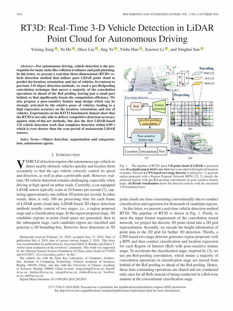
Fig. 1. The pipeline of RT3D: (a) a 3-D point cloud of LiDAR is projectedonto (b) a depth map in bird’s-eye view that is encoded with height informationof points. Then (c) a CNN-based two-stage detector is utilized to: 1) generateregion proposals with a Region Proposal Network (RPN) [2], 2) classify theproposed regions with pre-RoI-pooling convolutions on pose-sensitive featuremaps. (d) Result visualization shows the detected vehicles with the orientated3-D bounding boxes.
point clouds are time-consuming conventionally due to conductclassification and regression for thousands of candidate regions.
In this letter, we present a real-time vehicle detection methodRT3D. The pipeline of RT3D is shown in Fig. 1. Firstly, tomeet the input format requirement of the convolution neuralnetwork, we project the discrete 3D point cloud into a 2D gridrepresentation. Secondly, we encode the height information ofpoint data in the 2D grid for further 3D detection. Thirdly, aCNN-based two-stage detector generates region proposals witha RPN and then conduct classification and location regressionfor each Region of Interest (RoI) with pose-sensitive featuremaps. To accelerate the classification stage, inspired by [3], weuse pre-RoI-pooling convolution, which means a majority ofconvolution operations in classification stage are moved frombehind of the RoI pooling to ahead of the RoI pooling. Hence,these time-consuming operations are shared and are conductedonly once for all RoIs instead of being conducted in a RoI-wisemanner at the conventional classification stage.
2377-3766 © 2018 IEEE. Personal use is permitted, but republication/redistribution requires IEEE permission.See http://www.ieee.org/publications standards/publications/rights/index.html for more information.
ZENG et al.: RT3D: REAL-TIME 3-D VEHICLE DETECTION IN LIDAR POINT CLOUD FOR AUTONOMOUS DRIVING 3435
Benefited from the pre-RoI-pooling convolution and pose-sensitive feature map techniques, the RT3D achieves compara-ble detection accuracy against the state-of-the-art methods onthe KITTI benchmark dataset [1]. Moreover, to the best of ourknowledge, the RT3D is the first LiDAR-based 3D vehicle de-tection work that completes detection within 0.09 seconds and iseven shorter than the scan period of mainstream LiDAR sensors.
II. RELATED WORK
Convolutional neural networks improve object detection sig-nificantly. In Fast-RCNN [2], a Region Proposal Network (RPN)was proposed to generate high-quality candidate regions. ThenFaster-RCNN [4] becomes a de facto pipeline of CNN-based ob-ject detection. Afterwards, 2D object detector [3] was proposedto improve the detection accuracy, and [5], [6] were proposed toaccelerate the detection speed. Recently, researchers conducted3D object detection on RGB images. Chabot et al. [7] proposeda multi-task neural network to create coarse-to-fine object pro-posals and to estimate vehicle orientation and location through2D/3D point matching. Chen et al. [8] exploited stereo images toplace proposals in the form of 3D bounding boxes. The authorsalso extended their work to monocular image [9] by projectingcandidate 3D boxes to the image plane and scoring boxes viaprior knowledge.
Besides RGB images, deep learning based techniques alsoconducted 3D object detection in point clouds. Qi et al. [10]proposed a PointNet that directly took point cloud as input. Li[11] designed a 3D fully convolution neural network to generateregion proposals for 3D object detection. Engelcke et al. [12]proposed a sparse convolution layer to classify region proposalsgenerated by a sliding window. Zhou et al. [13] divided the pointcloud into 3D voxels, aggregated local voxel features throughvoxel feature encoding (VFE) layers, and transformed pointclouds into a high-dimensional volumetric representation.
Besides directly operating in the 3D space, some other detec-tion approaches projected the 3D point cloud onto a 2D plane.[9], [14], [15] constructed a compact 2D representation of 3Dpoint cloud from bird’s-eye view, while [16] placed 3D windowson a front-view range map for vehicle detection. Ref. [17] and[18] generated 3D region proposals from a stack of height mapsand conducted classification and location estimation via fusingfeatures extracted from LiDAR point clouds and RGB images.However, these methods are time-consuming, which limits thepractical usage of these methods in autonomous driving.
III. PROPOSED APPROACH
As illustrated in Fig. 1, the discrete 3D point cloud P = {pi =(x, y, z), i = 1, 2, . . .} is projected onto a 2D grid GN ×N onthe xy-plane with height information embedded. The 2D gridrepresentation is then fed into a convolution neural network toestimate the center location, orientation, and size of a vehicle.
A. 2D Grid Representation of 3D Point Cloud
Firstly, the 3D point cloud is projected onto a 2D grid inthe birds-eye view. As shown in Fig. 1, from (a) to (b), we
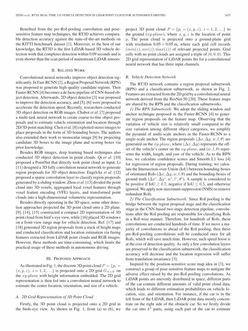
project 3D point cloud P = {pi = (x, y, z), i = 1, 2, . . .} tothe ground (xy-plane), where x, y, z is the location of pointp. The point cloud is projected onto a ground-plane gridwith resolution 0.05 × 0.05 m, where each grid cell records(min(z), ave(z),max(z)) of relevant projected points. Gridcells with no point clouds are assigned a triple of (0, 0, 0). This2D grid representation of LiDAR points fits for a convolutionalneural network that has three input channels.
B. Vehicle Detection Network
The RT3D network contains a region proposal subnetwork(RPN) and a classification subnetwork, as shown in Fig. 2.Features are extracted from the 2D grid by a convolutional neuralnetwork derived from the ResNet-50 [20]. These feature mapsare shared by the RPN and the classification subnetworks.
1) The RPN Subnetwork: We adopt the sliding window andanchor technique proposed in the Faster-RCNN [4] to gener-ate region proposals on the feature map. Observing that thevariation of vehicle size is relatively small compared to thesize variation among different object categories, we simplifythe pyramid of multi-scale anchors in the Faster-RCNN to asingle-scale anchor. The region proposals (Δx,Δy, w, l, θ) aregenerated on the xy-plane, where (Δx,Δy) represents the off-set of the vehicle’s center on the xy-plane, and (w, l, θ) repre-sents the width, length, and yaw of the vehicle. As to the RPNloss, we calculate confidence scores and Smooth L1 loss [4]for regression of region proposals. During training, we calcu-late the Intersection-over-Union (IoU) between bounding-boxesof orientated RoIs (Δx,Δy, w, l, θ) and the bounding-boxes ofground truth (Δx∗,Δy∗, w∗, l∗, θ∗). A sample is considered tobe positive if IoU ≥ 0.7, negative if IoU ≤ 0.5, and otherwiseignored. We apply non-maximum suppression (NMS) to removeredundant RoIs.
2) The Classification Subnetwork: Since RoI pooling is thebridge between the region proposal stage and the classificationstage in the CNN-based two-stage detection pipeline, convolu-tions after the RoI pooling are responsible for classifying RoIsin a RoI-wise manner. Therefore, for hundreds of RoIs, theseconvolutions are conducted hundreds of time. If we move a ma-jority of convolutions to ahead of the RoI pooling, then thesepre-RoI-pooling convolutions will be conducted once for allRoIs, which will save much time. However, such speed boost isat the cost of detection quality. As only a few convolution layersare preserved in the classification subnetwork, the classificationaccuracy will decrease and the location regression will sufferfrom translation-invariance [3].
Inspired by the position-sensitive score map idea in [3], weconstruct a group of pose-sensitive feature maps to mitigate theadverse effect raised by the pre-RoI-pooling convolutions. AsLiDAR points are unevenly distributed in space, different partsof the car contain different amounts of valid point cloud data,which leads to different estimation probabilities on vehicle lo-cation, size, and orientation. For instance, if the car is in theleft front of the LiDAR, then LiDAR point data mostly concen-trate on the right side of the obstacle car. So we firstly dividethe car into k2 parts, using each part of the car to estimate
3436 IEEE ROBOTICS AND AUTOMATION LETTERS, VOL. 3, NO. 4, OCTOBER 2018
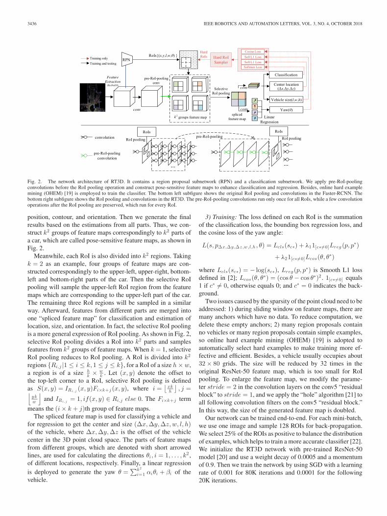
Fig. 2. The network architecture of RT3D. It contains a region proposal subnetwork (RPN) and a classification subnetwork. We apply pre-RoI-poolingconvolutions before the RoI pooling operation and construct pose-sensitive feature maps to enhance classification and regression. Besides, online hard examplemining (OHEM) [19] is employed to train the classifier. The bottom left subfigure shows the original RoI pooling and convolutions in the Faster-RCNN. Thebottom right subfigure shows the RoI pooling and convolutions in the RT3D. The pre-RoI-pooling convolutions run only once for all RoIs, while a few convolutionoperations after the RoI pooling are preserved, which run for every RoI.
position, contour, and orientation. Then we generate the finalresults based on the estimations from all parts. Thus, we con-struct k2 groups of feature maps correspondingly to k2 parts ofa car, which are called pose-sensitive feature maps, as shown inFig. 2.
Meanwhile, each RoI is also divided into k2 regions. Takingk = 2 as an example, four groups of feature maps are con-structed correspondingly to the upper-left, upper-right, bottom-left and bottom-right parts of the car. Then the selective RoIpooling will sample the upper-left RoI region from the featuremaps which are corresponding to the upper-left part of the car.The remaining three RoI regions will be sampled in a similarway. Afterward, features from different parts are merged intoone “spliced feature map” for classification and estimation oflocation, size, and orientation. In fact, the selective RoI poolingis a more general expression of RoI pooling. As shown in Fig. 2,selective RoI pooling divides a RoI into k2 parts and samplesfeatures from k2 groups of feature maps. When k = 1, selectiveRoI pooling reduces to RoI pooling. A RoI is divided into k2
regions {Ri,j |1 ≤ i ≤ k, 1 ≤ j ≤ k}, for a RoI of a size h × w,a region is of a size h
k × wk . Let (x, y) denote the offset to
the top-left corner to a RoI, selective RoI pooling is definedas S(x, y) = IRi , j
(x, y)Fi×k+j (x, y), where i =⌊
xkh
⌋, j =⌊
ykw
⌋and IRi , j
= 1, if(x, y) ∈ Ri,j else 0. The Fi×k+j term
means the (i × k + j)th group of feature maps.The spliced feature map is used for classifying a vehicle and
for regression to get the center and size (Δx,Δy,Δz, w, l, h)of the vehicle, where Δx,Δy,Δz is the offset of the vehiclecenter in the 3D point cloud space. The parts of feature mapsfrom different groups, which are denoted with short arrowedlines, are used for calculating the directions θi, i = 1, . . . , k2 ,of different locations, respectively. Finally, a linear regressionis deployed to generate the yaw θ =
∑k 2
i=1 αiθi + βi of thevehicle.
3) Training: The loss defined on each RoI is the summationof the classification loss, the bounding box regression loss, andthe cosine loss of the yaw angle:
L(s, pΔx,Δy ,Δz ,w ,l,h , θ) = Lcls(sc∗) + λ11[c∗�=0]Lreg (p, p∗)
+ λ21[c∗�=0]Lcos(θ, θ∗)
where Lcls(sc∗) = − log(sc∗), Lreg (p, p∗) is Smooth L1 lossdefined in [2]; Lcos(θ, θ∗) = (cos θ − cos θ∗)2 . 1[c∗�=0] equals1 if c∗ �= 0, otherwise equals 0; and c∗ = 0 indicates the back-ground.
Two issues caused by the sparsity of the point cloud need to beaddressed: 1) during sliding window on feature maps, there aremany anchors which have no data. To reduce computation, wedelete these empty anchors; 2) many region proposals containno vehicles or many region proposals contain simple examples,so online hard example mining (OHEM) [19] is adopted toautomatically select hard examples to make training more ef-fective and efficient. Besides, a vehicle usually occupies about32 × 80 grids. The size will be reduced by 32 times in theoriginal ResNet-50 feature map, which is too small for RoIpooling. To enlarge the feature map, we modify the parame-ter stride = 2 in the convolution layers on the conv5 “residualblock” to stride = 1, and we apply the “hole” algorithm [21] toall following convolution filters on the conv5 “residual block.”In this way, the size of the generated feature map is doubled.
Our network can be trained end-to-end. For each mini-batch,we use one image and sample 128 ROIs for back-propagation.We select 25% of the ROIs as positive to balance the distributionof examples, which helps to train a more accurate classifier [22].We initialize the RT3D network with pre-trained ResNet-50model [20] and use a weight decay of 0.0005 and a momentumof 0.9. Then we train the network by using SGD with a learningrate of 0.001 for 80K iterations and 0.0001 for the following20K iterations.
ZENG et al.: RT3D: REAL-TIME 3-D VEHICLE DETECTION IN LIDAR POINT CLOUD FOR AUTONOMOUS DRIVING 3437
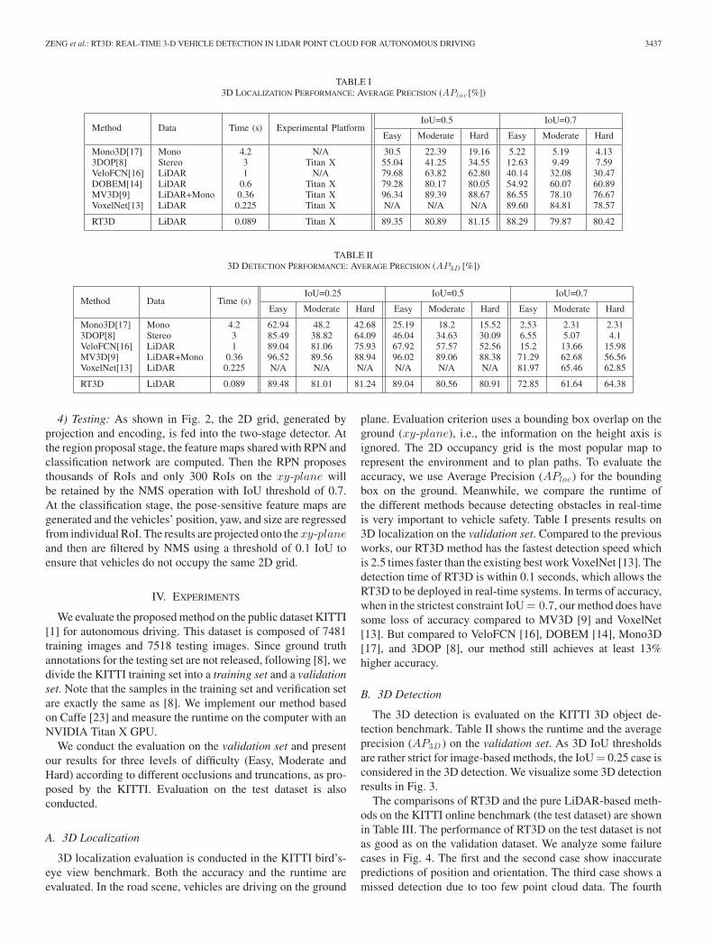
TABLE I3D LOCALIZATION PERFORMANCE: AVERAGE PRECISION (APloc [%])
TABLE II3D DETECTION PERFORMANCE: AVERAGE PRECISION (AP3D [%])
4) Testing: As shown in Fig. 2, the 2D grid, generated byprojection and encoding, is fed into the two-stage detector. Atthe region proposal stage, the feature maps shared with RPN andclassification network are computed. Then the RPN proposesthousands of RoIs and only 300 RoIs on the xy-plane willbe retained by the NMS operation with IoU threshold of 0.7.At the classification stage, the pose-sensitive feature maps aregenerated and the vehicles’ position, yaw, and size are regressedfrom individual RoI. The results are projected onto the xy-planeand then are filtered by NMS using a threshold of 0.1 IoU toensure that vehicles do not occupy the same 2D grid.
IV. EXPERIMENTS
We evaluate the proposed method on the public dataset KITTI[1] for autonomous driving. This dataset is composed of 7481training images and 7518 testing images. Since ground truthannotations for the testing set are not released, following [8], wedivide the KITTI training set into a training set and a validationset. Note that the samples in the training set and verification setare exactly the same as [8]. We implement our method basedon Caffe [23] and measure the runtime on the computer with anNVIDIA Titan X GPU.
We conduct the evaluation on the validation set and presentour results for three levels of difficulty (Easy, Moderate andHard) according to different occlusions and truncations, as pro-posed by the KITTI. Evaluation on the test dataset is alsoconducted.
A. 3D Localization
3D localization evaluation is conducted in the KITTI bird’s-eye view benchmark. Both the accuracy and the runtime areevaluated. In the road scene, vehicles are driving on the ground
plane. Evaluation criterion uses a bounding box overlap on theground (xy-plane), i.e., the information on the height axis isignored. The 2D occupancy grid is the most popular map torepresent the environment and to plan paths. To evaluate theaccuracy, we use Average Precision (APloc ) for the boundingbox on the ground. Meanwhile, we compare the runtime ofthe different methods because detecting obstacles in real-timeis very important to vehicle safety. Table I presents results on3D localization on the validation set. Compared to the previousworks, our RT3D method has the fastest detection speed whichis 2.5 times faster than the existing best work VoxelNet [13]. Thedetection time of RT3D is within 0.1 seconds, which allows theRT3D to be deployed in real-time systems. In terms of accuracy,when in the strictest constraint IoU = 0.7, our method does havesome loss of accuracy compared to MV3D [9] and VoxelNet[13]. But compared to VeloFCN [16], DOBEM [14], Mono3D[17], and 3DOP [8], our method still achieves at least 13%higher accuracy.
B. 3D Detection
The 3D detection is evaluated on the KITTI 3D object de-tection benchmark. Table II shows the runtime and the averageprecision (AP3D ) on the validation set. As 3D IoU thresholdsare rather strict for image-based methods, the IoU = 0.25 case isconsidered in the 3D detection. We visualize some 3D detectionresults in Fig. 3.
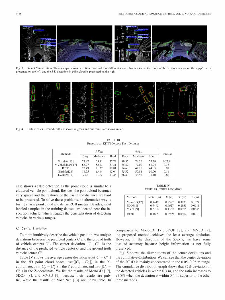
The comparisons of RT3D and the pure LiDAR-based meth-ods on the KITTI online benchmark (the test dataset) are shownin Table III. The performance of RT3D on the test dataset is notas good as on the validation dataset. We analyze some failurecases in Fig. 4. The first and the second case show inaccuratepredictions of position and orientation. The third case shows amissed detection due to too few point cloud data. The fourth
3438 IEEE ROBOTICS AND AUTOMATION LETTERS, VOL. 3, NO. 4, OCTOBER 2018
Fig. 3. Result Visualization. This example shows detection results of four different scenes. In each scene, the result of the 3-D localization on the xy-plane ispresented on the left, and the 3-D detection in point cloud is presented on the right.
Fig. 4. Failure cases. Ground-truth are shown in green and our results are shown in red.
TABLE IIIRESULTS ON KITTI ONLINE TEST DATASET
case shows a false detection as the point cloud is similar to acluttered vehicle point cloud. Besides, the point cloud becomesvery sparse and the features of the car in the distance are hardto be preserved. To solve these problems, an alternative way isfusing sparse point cloud and dense RGB images. Besides, mostlabeled samples in the training dataset are located near the in-spection vehicle, which negates the generalization of detectingvehicles in various ranges.
C. Center Deviation
To more intuitively describe the vehicle position, we analyzedeviations between the predicted centers C and the ground truthof vehicle centers C∗. The center deviation |C − C∗| is thedistance of the predicted vehicle center C and the ground truthvehicle center C∗.
Table IV shows the average center deviation ave(|C − C∗|)in the 3D point cloud space, ave(|Cx − C∗
x |) in the X-coordinate, ave(|Cy − C∗
y |) in the Y-coordinate, and ave(|Cz −C∗
z |) in the Z-coordinate. We list the results of Mono3D [17],3DOP [8], and MV3D [9], because their results are pub-lic, while the results of VoxelNet [13] are unavailable. In
TABLE IVVEHICLES CENTER DEVIATION
comparison to Mono3D [17], 3DOP [8], and MV3D [9],the proposed method achieves the least average deviation.However, in the direction of the Z-axis, we have someloss of accuracy because height information is not fullypreserved.
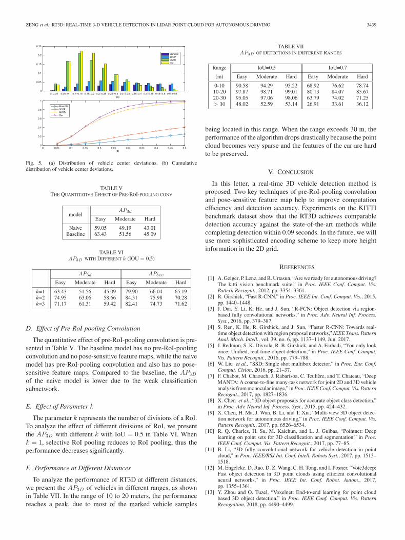
Fig. 5 shows the distributions of the center deviations andthe cumulative distribution. We can see that the center deviationof the RT3D is mainly concentrated in the 0.05–0.25 m range.The cumulative distribution graph shows that 87% deviation ofthe detected vehicles is within 0.3 m, and the ratio increases to97.8% when the deviation is within 0.4 m, superior to the otherthree methods.
ZENG et al.: RT3D: REAL-TIME 3-D VEHICLE DETECTION IN LIDAR POINT CLOUD FOR AUTONOMOUS DRIVING 3439
Fig. 5. (a) Distribution of vehicle center deviations. (b) Cumulativedistribution of vehicle center deviations.
TABLE VTHE QUANTITATIVE EFFECT OF PRE-ROI-POOLING CONV
TABLE VIAP3D WITH DIFFERENT k (IOU = 0.5)
D. Effect of Pre-RoI-pooling Convolution
The quantitative effect of pre-RoI-pooling convolution is pre-sented in Table V. The baseline model has no pre-RoI-poolingconvolution and no pose-sensitive feature maps, while the naivemodel has pre-RoI-pooling convolution and also has no pose-sensitive feature maps. Compared to the baseline, the AP3D
of the naive model is lower due to the weak classificationsubnetwork.
E. Effect of Parameter k
The parameter k represents the number of divisions of a RoI.To analyze the effect of different divisions of RoI, we presentthe AP3D with different k with IoU = 0.5 in Table VI. Whenk = 1, selective RoI pooling reduces to RoI pooling, thus theperformance decreases significantly.
F. Performance at Different Distances
To analyze the performance of RT3D at different distances,we present the AP3D of vehicles in different ranges, as shownin Table VII. In the range of 10 to 20 meters, the performancereaches a peak, due to most of the marked vehicle samples
TABLE VIIAP3D OF DETECTIONS IN DIFFERENT RANGES
being located in this range. When the range exceeds 30 m, theperformance of the algorithm drops drastically because the pointcloud becomes very sparse and the features of the car are hardto be preserved.
V. CONCLUSION
In this letter, a real-time 3D vehicle detection method isproposed. Two key techniques of pre-RoI-pooling convolutionand pose-sensitive feature map help to improve computationefficiency and detection accuracy. Experiments on the KITTIbenchmark dataset show that the RT3D achieves comparabledetection accuracy against the state-of-the-art methods whilecompleting detection within 0.09 seconds. In the future, we willuse more sophisticated encoding scheme to keep more heightinformation in the 2D grid.
REFERENCES
[1] A. Geiger, P. Lenz, and R. Urtasun, “Are we ready for autonomous driving?The kitti vision benchmark suite,” in Proc. IEEE Conf. Comput. Vis.Pattern Recognit., 2012, pp. 3354–3361.
[2] R. Girshick, “Fast R-CNN,” in Proc. IEEE Int. Conf. Comput. Vis., 2015,pp. 1440–1448.
[3] J. Dai, Y. Li, K. He, and J. Sun, “R-FCN: Object detection via region-based fully convolutional networks,” in Proc. Adv. Neural Inf. Process.Syst., 2016, pp. 379–387.
[4] S. Ren, K. He, R. Girshick, and J. Sun, “Faster R-CNN: Towards real-time object detection with region proposal networks,” IEEE Trans. PatternAnal. Mach. Intell., vol. 39, no. 6, pp. 1137–1149, Jun. 2017.
[5] J. Redmon, S. K. Divvala, R. B. Girshick, and A. Farhadi, “You only lookonce: Unified, real-time object detection,” in Proc. IEEE Conf. Comput.Vis. Pattern Recognit., 2016, pp. 779–788.
[6] W. Liu et al., “SSD: Single shot multibox detector,” in Proc. Eur. Conf.Comput. Cision, 2016, pp. 21–37.
[7] F. Chabot, M. Chaouch, J. Rabarisoa, C. Teuliere, and T. Chateau, “DeepMANTA: A coarse-to-fine many-task network for joint 2D and 3D vehicleanalysis from monocular image,” in Proc. IEEE Conf. Comput. Vis. PatternRecognit., 2017, pp. 1827–1836.
[8] X. Chen et al., “3D object proposals for accurate object class detection,”in Proc. Adv. Neural Inf. Process. Syst., 2015, pp. 424–432.
[9] X. Chen, H. Ma, J. Wan, B. Li, and T. Xia, “Multi-view 3D object detec-tion network for autonomous driving,” in Proc. IEEE Conf. Comput. Vis.Pattern Recognit., 2017, pp. 6526–6534.
[10] R. Q. Charles, H. Su, M. Kaichun, and L. J. Guibas, “Pointnet: Deeplearning on point sets for 3D classification and segmentation,” in Proc.IEEE Conf. Comput. Vis. Pattern Recognit., 2017, pp. 77–85.
[11] B. Li, “3D fully convolutional network for vehicle detection in pointcloud,” in Proc. IEEE/RSJ Int. Conf. Intell. Robots Syst., 2017, pp. 1513–1518.
[12] M. Engelcke, D. Rao, D. Z. Wang, C. H. Tong, and I. Posner, “Vote3deep:Fast object detection in 3D point clouds using efficient convolutionalneural networks,” in Proc. IEEE Int. Conf. Robot. Autom., 2017,pp. 1355–1361.
[13] Y. Zhou and O. Tuzel, “Voxelnet: End-to-end learning for point cloudbased 3D object detection,” in Proc. IEEE Conf. Comput. Vis. PatternRecognition, 2018, pp. 4490–4499.
3440 IEEE ROBOTICS AND AUTOMATION LETTERS, VOL. 3, NO. 4, OCTOBER 2018
[14] S. L. Yu, T. Westfechtel, R. Hamada, K. Ohno, and S. Tadokoro, “Vehicledetection and localization on bird’s eye view elevation images using con-volutional neural network,” in Proc. IEEE Int. Symp. Safet. Secur. RescueRobot., 2017, pp. 102–109.
[15] A. Asvadi, L. Garrote, C. Premebida, P. Peixoto, and U. J. Nunes,“Depthcn: Vehicle detection using 3D-lidar and convnet,” in Proc. IEEEInt. Conf. Intell. Transp. Syst., Oct. 2017, pp. 1–6.
[16] B. Li, T. Zhang, and T. Xia, “Vehicle detection from 3D lidar using fullyconvolutional network,” in Proc. Robotics: Sci. Syst., 2016, pp. 18–22.
[17] X. Chen, K. Kundu, Z. Zhang, H. Ma, S. Fidler, and R. Urtasun, “Monoc-ular 3D object detection for autonomous driving,” in Proc. IEEE Conf.Comput. Vis. Pattern Recognit., 2016, pp. 2147–2156.
[18] J. Ku, M. Mozifian, J. Lee, A. Harakeh, and S. Waslander, “Joint3D proposal generation and object detection from view aggregation,”arXiv:1712.02294, 2017.
[19] A. Shrivastava, A. Gupta, and R. Girshick, “Training region-based objectdetectors with online hard example mining,” in Proc. IEEE Conf. Comput.Vis. Pattern Recognit., 2016, pp. 761–769.
[20] K. He, X. Zhang, S. Ren, and J. Sun, “Deep residual learning for imagerecognition,” in Proc. IEEE Conf. Comput. Vis. Pattern Recognit., 2016,pp. 770–778.
[21] L. C. Chen, G. Papandreou, I. Kokkinos, K. Murphy, and A. L. Yuille,“Deeplab: Semantic image segmentation with deep convolutional nets,atrous convolution, and fully connected crfs,” IEEE Trans. Pattern Anal.Mach. Intell., vol. 40, no. 4, pp. 834–848, Apr. 2018.
[22] J. Hosang, R. Benenson, P. Dollar, and B. Schiele, “What Makes forEffective Detection Proposals?” IEEE Trans. Pattern Anal. Mach. Intell.,vol. 38, no. 4, pp. 814–830, Apr. 2016.
[23] Y. Jia et al., “Caffe: Convolutional architecture for fast feature embed-ding,” in Proc. ACM Int. Conf. Multimedia, 2014, pp. 675–678.
[24] J. Beltran, C. Guindel, F. M. Moreno, D. Cruzado, F. Garcia, and A. dela Escalera, “BirdNet: A 3D object detection framework from LiDARinformation,” arXiv:1805.01195.