Sampling from log-concave densityjps.math.cnrs.fr/slides/Durmus.pdf · Sampling from log-concave density Non-smooth potentials Numerical illustrations Conclusion When (k) k 1 is nonincreasing

MotivationFramework

Sampling from strongly log-concave densitySampling from log-concave density

Non-smooth potentialsNumerical illustrations

Conclusion

Sampling from log-concave density

Alain Durmus, Eric Moulines, Marcelo Pereyra

Telecom ParisTech, Ecole Polytechnique, Bristol University

A. Durmus, Eric Moulines, Marcelo Pereyra Seminaire des jeunes probabilistes et statisticiens-2016

MotivationFramework



Conclusion

1 Motivation

2 Framework

3 Sampling from strongly log-concave density

4 Sampling from log-concave density

5 Non-smooth potentials

6 Numerical illustrations

7 Conclusion


MotivationFramework



Conclusion

Introduction

Sampling distribution over high-dimensional state-space has recentlyattracted a lot of research efforts in computational statistics andmachine learning community...

Applications (non-exhaustive)

1 Bayesian inference for high-dimensional models and Bayesian nonparametrics

2 Bayesian linear inverse problems (typically function space problemsconverted to high-dimensional problem by Galerkin method)

3 Aggregation of estimators and experts

Most of the sampling techniques known so far do not scale tohigh-dimension... Challenges are numerous in this area...


MotivationFramework



Conclusion

Bayesian setting (I)

- In a Bayesian setting, a parameter βββ ∈ Rd is embedded with a priordistribution ξ and the observations are given by a probabilistic model:

Y ∼ `(·|βββ)

The inference is then based on the posterior distribution:

π(dβββ|Y ) =ξ(dβββ)`(Y |βββ)∫`(Y |u)ξ(du)

.

In most cases the normalizing constant is not tractable:

π(dβββ|Y ) ∝ ξ(dβββ)`(Y |βββ) .


MotivationFramework



Conclusion

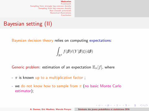
Bayesian setting (II)

Bayesian decision theory relies on computing expectations:∫Rdf(βββ)`(Y |βββ)ξ(dβββ)

Generic problem: estimation of an expectation Eπ[f ], where

- π is known up to a multiplicative factor ;

- we do not know how to sample from π (no basic Monte Carloestimator);


MotivationFramework



Conclusion

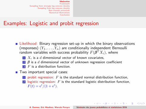
Examples: Logistic and probit regression

Likelihood: Binary regression set-up in which the binary observations(responses) (Y1, . . . , Yn) are conditionally independent Bernoullirandom variables with success probability F (βββTXi), where

1 Xi is a d dimensional vector of known covariates,2 βββ is a d dimensional vector of unknown regression coefficient3 F is a distribution function.

Two important special cases:

1 probit regression: F is the standard normal distribution function,2 logistic regression: F is the standard logistic distribution function,F (t) = et/(1 + et).


MotivationFramework



Conclusion

Examples: Logistic and probit regression

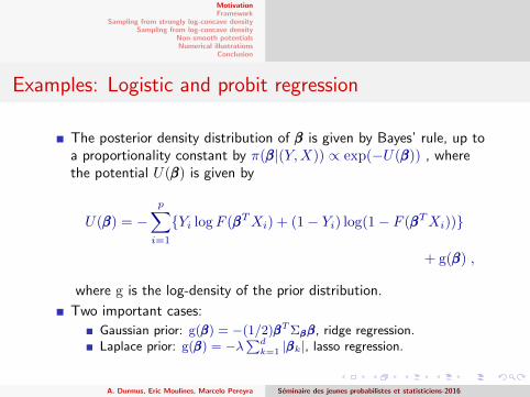
The posterior density distribution of βββ is given by Bayes’ rule, up toa proportionality constant by π(βββ|(Y,X)) ∝ exp(−U(βββ)) , wherethe potential U(βββ) is given by

U(βββ) = −p∑i=1

{Yi logF (βββTXi) + (1− Yi) log(1− F (βββTXi))}

+ g(βββ) ,

where g is the log-density of the prior distribution.

Two important cases:

Gaussian prior: g(βββ) = −(1/2)βββTΣββββββ, ridge regression.Laplace prior: g(βββ) = −λ

∑dk=1 |βββk|, lasso regression.


MotivationFramework



Conclusion

New challenges

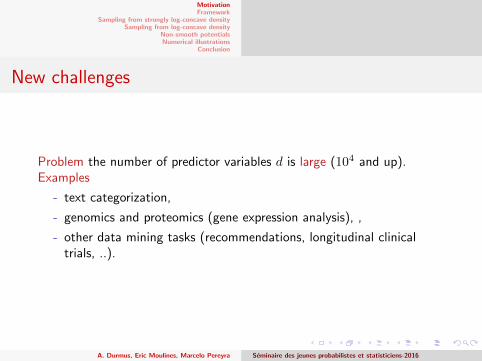
Problem the number of predictor variables d is large (104 and up).Examples

- text categorization,

- genomics and proteomics (gene expression analysis), ,

- other data mining tasks (recommendations, longitudinal clinicaltrials, ..).


MotivationFramework



Conclusion

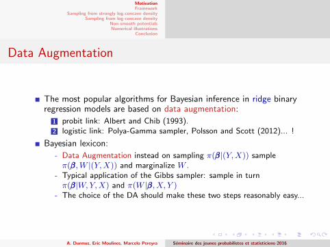
Data Augmentation

The most popular algorithms for Bayesian inference in ridge binaryregression models are based on data augmentation:

1 probit link: Albert and Chib (1993).2 logistic link: Polya-Gamma sampler, Polsson and Scott (2012)... !

Bayesian lexicon:

- Data Augmentation instead on sampling π(βββ|(Y,X)) sampleπ(βββ,W |(Y,X)) and marginalize W .

- Typical application of the Gibbs sampler: sample in turnπ(βββ|W,Y,X) and π(W |βββ,X, Y )

- The choice of the DA should make these two steps reasonably easy...


MotivationFramework



Conclusion

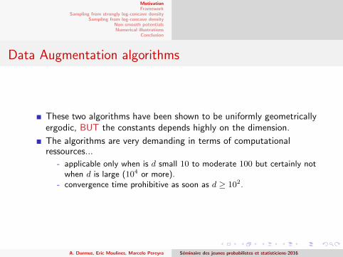
Data Augmentation algorithms

These two algorithms have been shown to be uniformly geometricallyergodic, BUT the constants depends highly on the dimension.

The algorithms are very demanding in terms of computationalressources...

- applicable only when is d small 10 to moderate 100 but certainly notwhen d is large (104 or more).

- convergence time prohibitive as soon as d ≥ 102.


MotivationFramework



Conclusion

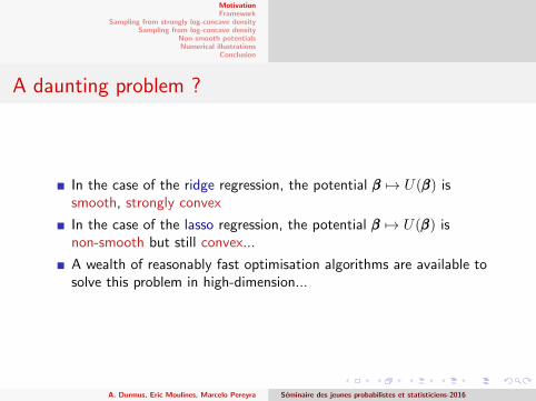
A daunting problem ?

In the case of the ridge regression, the potential βββ 7→ U(βββ) issmooth, strongly convex

In the case of the lasso regression, the potential βββ 7→ U(βββ) isnon-smooth but still convex...

A wealth of reasonably fast optimisation algorithms are available tosolve this problem in high-dimension...


MotivationFramework



Conclusion

1 Motivation

2 Framework





7 Conclusion


MotivationFramework



Conclusion

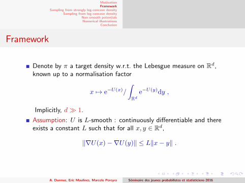
Framework

Denote by π a target density w.r.t. the Lebesgue measure on Rd,known up to a normalisation factor

x 7→ e−U(x)/

∫Rd

e−U(y)dy ,

Implicitly, d� 1.

Assumption: U is L-smooth : continuously differentiable and thereexists a constant L such that for all x, y ∈ Rd,

‖∇U(x)−∇U(y)‖ ≤ L‖x− y‖ .


MotivationFramework



Conclusion

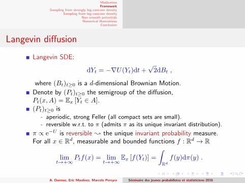
Langevin diffusion

Langevin SDE:

dYt = −∇U(Yt)dt+√

2dBt ,

where (Bt)t≥0 is a d-dimensional Brownian Motion.

Denote by (Pt)t≥0 the semigroup of the diffusion,Pt(x,A) = Ex [Yt ∈ A].(Pt)t≥0 is

- aperiodic, strong Feller (all compact sets are small).- reversible w.r.t. to π (admits π as its unique invariant distribution).

π ∝ e−U is reversible ; the unique invariant probability measure.For all x ∈ Rd, measurable and bounded functions f : Rd → R

limt→+∞

Ptf(x) = limt→+∞

Ex [f(Yt)] =

∫Rdf(y)dπ(y) .


MotivationFramework



Conclusion

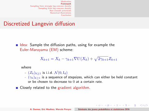
Discretized Langevin diffusion

Idea: Sample the diffusion paths, using for example theEuler-Maruyama (EM) scheme:

Xk+1 = Xk − γk+1∇U(Xk) +√

2γk+1Zk+1

where

- (Zk)k≥1 is i.i.d. N (0, Id)- (γk)k≥1 is a sequence of stepsizes, which can either be held constant

or be chosen to decrease to 0 at a certain rate.

Closely related to the gradient algorithm.


MotivationFramework



Conclusion

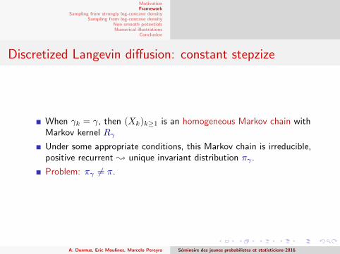
Discretized Langevin diffusion: constant stepzize

When γk = γ, then (Xk)k≥1 is an homogeneous Markov chain withMarkov kernel Rγ

Under some appropriate conditions, this Markov chain is irreducible,positive recurrent ; unique invariant distribution πγ .

Problem: πγ 6= π.


MotivationFramework



Conclusion

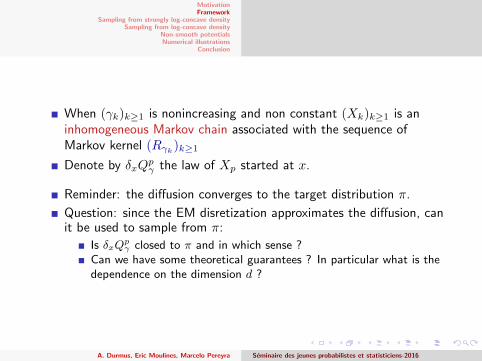
When (γk)k≥1 is nonincreasing and non constant (Xk)k≥1 is aninhomogeneous Markov chain associated with the sequence ofMarkov kernel (Rγk)k≥1

Denote by δxQpγ the law of Xp started at x.

Reminder: the diffusion converges to the target distribution π.

Question: since the EM disretization approximates the diffusion, canit be used to sample from π:

Is δxQpγ closed to π and in which sense ?

Can we have some theoretical guarantees ? In particular what is thedependence on the dimension d ?


MotivationFramework



Conclusion

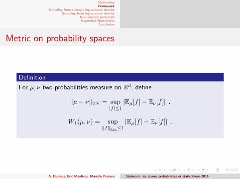
Metric on probability spaces

Definition

For µ, ν two probabilities measure on Rd, define

‖µ− ν‖TV = sup|f |≤1

|Eµ[f ]− Eν [f ]| .

W1(µ, ν) = sup‖f‖Lip≤1

|Eµ[f ]− Eν [f ]| .


MotivationFramework



Conclusion

1 Motivation

2 Framework





7 Conclusion


MotivationFramework



Conclusion

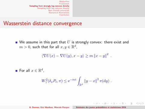
Wasserstein distance convergence

We assume in this part that U is strongly convex: there exist andm > 0, such that for all x, y ∈ Rd,

〈∇U(x)−∇U(y), x− y〉 ≥ m ‖x− y‖2 .

For all x ∈ Rd,

W 21 (δxPt, π) ≤ e−mt

∫Rd‖y − x‖2 π(dy) .


MotivationFramework



Conclusion

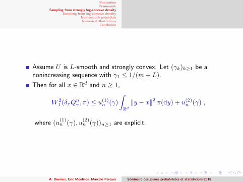
Assume U is L-smooth and strongly convex. Let (γk)k≥1 be anonincreasing sequence with γ1 ≤ 1/(m+ L).

Then for all x ∈ Rd and n ≥ 1,

W 21 (δxQ

nγ , π) ≤ u(1)

n (γ)

∫Rd‖y − x‖2 π(dy) + u(2)

n (γ) ,

where (u(1)n (γ), u

(2)n (γ))n≥1 are explicit.


MotivationFramework



Conclusion

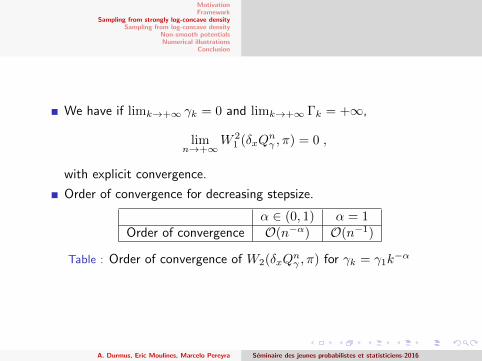
We have if limk→+∞ γk = 0 and limk→+∞ Γk = +∞,

limn→+∞

W 21 (δxQ

nγ , π) = 0 ,

with explicit convergence.

Order of convergence for decreasing stepsize.

α ∈ (0, 1) α = 1Order of convergence O(n−α) O(n−1)

Table : Order of convergence of W2(δxQnγ , π) for γk = γ1k

−α


MotivationFramework



Conclusion

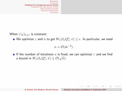
When (γk)k≥1 is constant:

We optimize γ and n to get W1(δxQnγ , π) ≤ ε. In particular, we need

n = O(dε−2) .

If the number of iterations n is fixed, we can optimize γ and we finda bound in W1(δxQ

nγ , π) ≤ O(

√n).


MotivationFramework



Conclusion

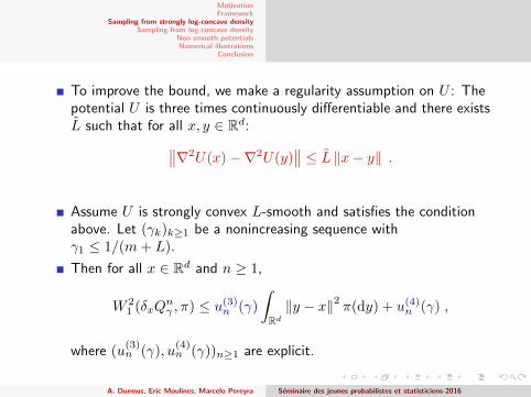
To improve the bound, we make a regularity assumption on U : Thepotential U is three times continuously differentiable and there existsL such that for all x, y ∈ Rd:∥∥∇2U(x)−∇2U(y)

∥∥ ≤ L ‖x− y‖ .Assume U is strongly convex L-smooth and satisfies the conditionabove. Let (γk)k≥1 be a nonincreasing sequence withγ1 ≤ 1/(m+ L).

Then for all x ∈ Rd and n ≥ 1,

W 21 (δxQ

nγ , π) ≤ u(3)

n (γ)

∫Rd‖y − x‖2 π(dy) + u(4)

n (γ) ,

where (u(3)n (γ), u

(4)n (γ))n≥1 are explicit.


MotivationFramework



Conclusion

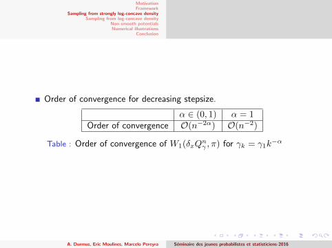
Order of convergence for decreasing stepsize.

α ∈ (0, 1) α = 1Order of convergence O(n−2α) O(n−2)

Table : Order of convergence of W1(δxQnγ , π) for γk = γ1k

−α


MotivationFramework



Conclusion

When (γk)k≥1 is constant:

We optimize γ and n to get W1(δxQnγ , π) ≤ ε. In particular, we need

n = O(√dε−1) .

If the number of iterations n is fixed, we can optimize γ and we finda bound in W1(δxQ

nγ , π) ≤ O(n−1).


MotivationFramework



Conclusion

1 Motivation

2 Framework





7 Conclusion


MotivationFramework



Conclusion

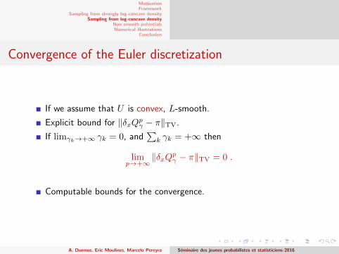
Convergence of the Euler discretization

If we assume that U is convex, L-smooth.

Explicit bound for ‖δxQpγ − π‖TV.

If limγk→+∞ γk = 0, and∑k γk = +∞ then

limp→+∞

‖δxQpγ − π‖TV = 0 .

Computable bounds for the convergence.


MotivationFramework



Conclusion

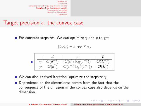
Target precision ε: the convex case

For constant stepsizes, We can optimize γ and p to get

‖δxQpγ − π‖TV ≤ ε .

d ε Lγ O(d−4) O(ε2/ log(ε−1)) O(L−2)

p O(d7) O(ε−2 log2(ε−1)) O(L2)

We can also at fixed iteration, optimize the stepsize γ.

Dependence on the dimensions: comes from the fact that theconvergence of the diffusion in the convex case also depends on thedimension.


MotivationFramework



Conclusion

1 Motivation

2 Framework





7 Conclusion


MotivationFramework



Conclusion

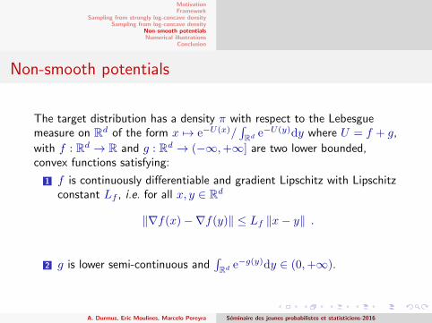
Non-smooth potentials

The target distribution has a density π with respect to the Lebesguemeasure on Rd of the form x 7→ e−U(x)/

∫Rd e−U(y)dy where U = f + g,

with f : Rd → R and g : Rd → (−∞,+∞] are two lower bounded,convex functions satisfying:

1 f is continuously differentiable and gradient Lipschitz with Lipschitzconstant Lf , i.e. for all x, y ∈ Rd

‖∇f(x)−∇f(y)‖ ≤ Lf ‖x− y‖ .

2 g is lower semi-continuous and∫Rd e−g(y)dy ∈ (0,+∞).


MotivationFramework



Conclusion

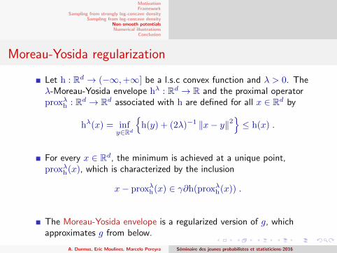
Moreau-Yosida regularization

Let h : Rd → (−∞,+∞] be a l.s.c convex function and λ > 0. Theλ-Moreau-Yosida envelope hλ : Rd → R and the proximal operatorproxλh : Rd → Rd associated with h are defined for all x ∈ Rd by

hλ(x) = infy∈Rd

{h(y) + (2λ)−1 ‖x− y‖2

}≤ h(x) .

For every x ∈ Rd, the minimum is achieved at a unique point,proxλh(x), which is characterized by the inclusion

x− proxλh(x) ∈ γ∂h(proxλh(x)) .

The Moreau-Yosida envelope is a regularized version of g, whichapproximates g from below.


MotivationFramework



Conclusion

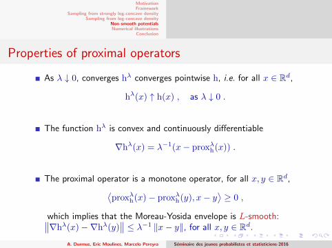
Properties of proximal operators

As λ ↓ 0, converges hλ converges pointwise h, i.e. for all x ∈ Rd,

hλ(x) ↑ h(x) , as λ ↓ 0 .

The function hλ is convex and continuously differentiable

∇hλ(x) = λ−1(x− proxλh(x)) .

The proximal operator is a monotone operator, for all x, y ∈ Rd,⟨proxλh(x)− proxλh(y), x− y

⟩≥ 0 ,

which implies that the Moreau-Yosida envelope is L-smooth:∥∥∇hλ(x)−∇hλ(y)∥∥ ≤ λ−1 ‖x− y‖, for all x, y ∈ Rd.


MotivationFramework



Conclusion

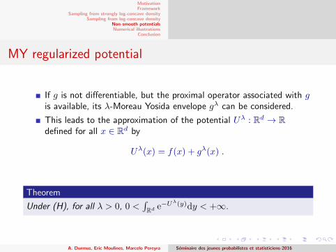
MY regularized potential

If g is not differentiable, but the proximal operator associated with gis available, its λ-Moreau Yosida envelope gλ can be considered.

This leads to the approximation of the potential Uλ : Rd → Rdefined for all x ∈ Rd by

Uλ(x) = f(x) + gλ(x) .

Theorem

Under (H), for all λ > 0, 0 <∫Rd e−U

λ(y)dy < +∞.


MotivationFramework



Conclusion

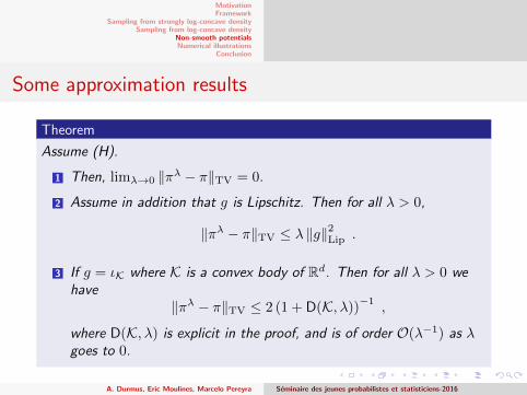
Some approximation results

Theorem

Assume (H).

1 Then, limλ→0 ‖πλ − π‖TV = 0.

2 Assume in addition that g is Lipschitz. Then for all λ > 0,

‖πλ − π‖TV ≤ λ ‖g‖2Lip .

3 If g = ιK where K is a convex body of Rd. Then for all λ > 0 wehave

‖πλ − π‖TV ≤ 2 (1 + D(K, λ))−1

,

where D(K, λ) is explicit in the proof, and is of order O(λ−1) as λgoes to 0.


MotivationFramework



Conclusion

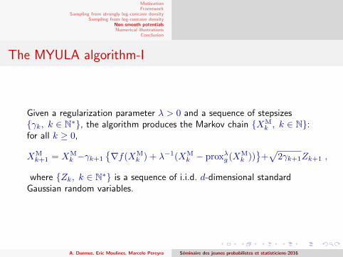
The MYULA algorithm-I

Given a regularization parameter λ > 0 and a sequence of stepsizes{γk, k ∈ N∗}, the algorithm produces the Markov chain {XM

k , k ∈ N}:for all k ≥ 0,

XMk+1 = XM

k −γk+1

{∇f(XM

k ) + λ−1(XMk − proxλg (XM

k ))}

+√

2γk+1Zk+1 ,

where {Zk, k ∈ N∗} is a sequence of i.i.d. d-dimensional standardGaussian random variables.


MotivationFramework



Conclusion

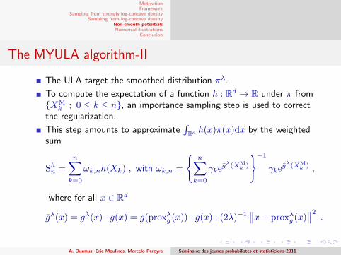
The MYULA algorithm-II

The ULA target the smoothed distribution πλ.

To compute the expectation of a function h : Rd → R under π from{XM

k ; 0 ≤ k ≤ n}, an importance sampling step is used to correctthe regularization.

This step amounts to approximate∫Rd h(x)π(x)dx by the weighted

sum

Shn =

n∑k=0

ωk,nh(Xk) , with ωk,n =

{n∑k=0

γkegλ(XM

k )

}−1

γkegλ(XM

k ) ,

where for all x ∈ Rd

gλ(x) = gλ(x)−g(x) = g(proxλg (x))−g(x)+(2λ)−1∥∥x− proxλg (x)

∥∥2.


MotivationFramework



Conclusion

1 Motivation

2 Framework





7 Conclusion


MotivationFramework



Conclusion

Image deconvolution

Objective recover an original image x ∈ Rn from a blurred and noisyobserved image y ∈ Rn related to x by the linear observation modely = Hx + w, where H is a linear operator representing the blurpoint spread function and w is a Gaussian vector with zero-meanand covariance matrix σ2In.

This inverse problem is usually ill-posed or ill-conditioned: exploitsprior knowledge about x.

One of the most widely used image prior for deconvolution problemsis the improper total-variation norm prior, π(x) ∝ exp (−α‖∇dx‖1),where ∇d denotes the discrete gradient operator that computes thevertical and horizontal differences between neighbour pixels.

π(x|y) ∝ exp[−‖y −Hx‖2/2σ2 − α‖∇dx‖1

].


MotivationFramework



Conclusion

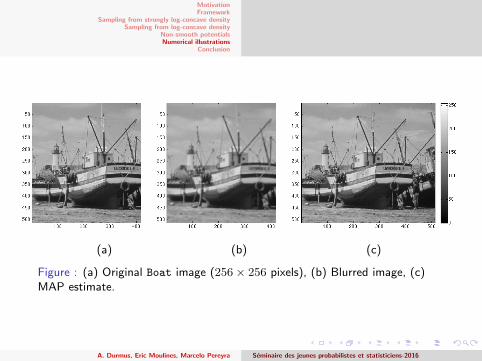
(a) (b) (c)

Figure : (a) Original Boat image (256× 256 pixels), (b) Blurred image, (c)MAP estimate.


MotivationFramework



Conclusion

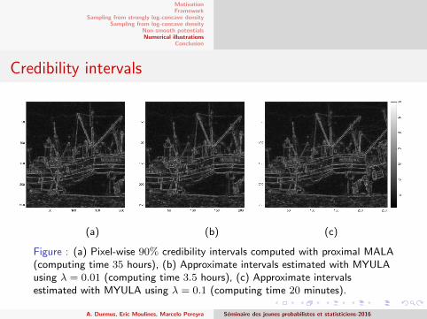
Credibility intervals

(a) (b) (c)

Figure : (a) Pixel-wise 90% credibility intervals computed with proximal MALA(computing time 35 hours), (b) Approximate intervals estimated with MYULAusing λ = 0.01 (computing time 3.5 hours), (c) Approximate intervalsestimated with MYULA using λ = 0.1 (computing time 20 minutes).


MotivationFramework



Conclusion

1 Motivation

2 Framework





7 Conclusion


MotivationFramework



Conclusion

What’s next ?

Extension of this work

- Richardson-Romberg interpolation: debiaising for smoothfunctionnals with non-asymptotic bounds on the MSE.

- Langevin meets Gibbs: ULA within Gibbs.- detailed comparison with MALA

Thank you for your attention.


Documents

Sampling from log-concave densityjps.math.cnrs.fr/slides/Durmus.pdf · Sampling from log-concave density Non-smooth potentials Numerical illustrations Conclusion When (k) k 1 is nonincreasing