Quantum Multiverses∗

James B. Hartle†

Santa Fe Institute, Santa Fe, NM 87501 and

Department of Physics, University of California,Santa Barbara, CA 93106-9530

(Dated: January 29, 2018)

Abstract

A quantum theory of the universe consists of a theory of its quantum dynamics (H) and a theory

of its quantum state (Ψ). The theory (H,Ψ) predicts quantum multiverses in the form of decoher-

ent sets of alternative histories describing the evolution of the universe’s spacetime geometry and

matter content. A small part of one of these histories is observed by us. These consequences follow:

(a) The universe generally exhibits different quantum multiverses at different levels and kinds of

coarse graining. (b) Quantum multiverses are not a choice or an assumption but are consequences

of (H,Ψ) or not. (c) Quantum multiverses are generic for simple (H,Ψ). (d) Anthropic selection

is automatic because observers are physical systems within the universe not somehow outside it.

(e) Quantum multiverses can provide different mechanisms for the variation constants in effective

theories (like the cosmological constant) enabling anthropic selection. (f) Different levels of coarse

grained multiverses provide different routes to calculation as a consequence of decoherence. We

support these conclusions by analyzing the quantum multiverses of a variety of quantum cosmo-

logical models aimed at the prediction of observable properties of our universe. In particular we

show how the example of a multiverse consisting of a vast classical spacetime containing many

pocket universes having different values of the fundamental constants arises automatically as part

of a quantum multiverse describing an eternally inflating false vacuum that decays by the quan-

tum nucleation of true vacuum bubbles. In a FAQ we argue that the quantum multiverses of the

universe are scientific, real, testable, falsifiable, and similar to those in other areas of science even

if they are not directly observable on arbitrarily large scales.

∗ A pedagogical essay.†Electronic address: hartle@physics.ucsb.edu

1

arX

iv:1

801.

0863

1v1

[gr

-qc]

25

Jan

2018

Contents

I. Introduction 3

II. Quantum Mechanics for the Universe Illustrated in Two-Slit Models 5

A. Simple Two Slit Model (TSS) 8

B. Two-slit Model with Gas (TSG): 10

C. Two-slit Model with Gas and Observer (TSGO) 12

1. Third and First Person Probabilities 12

2. Anthropic Selection 12

III. Five Exemplary Quantum Cosmological Multiverses 14

A. Common Elements 14

1. General Theory 15

IV. A Quantum Multiverse of Homogeneous, Isotropi, Classical Histories 16

1. Probabilities for Inflation 18

2. How this Model Supports the Conclusions 19

V. Quantum Multiverses of Pocket Universes 20

VI. A Quantum Multiverse of the Observable Properties of Our Bubble 22

A. Different Dynamics, Different Multiverses 24

VII. A Quantum Multiverse of Homogeneous and Isotropic Classical

Histories with Different Physical Constants 25

VIII. A Quantum Multiverse of Histories with Different CMBs 28

IX. Conclusions 29

A. General Conclusions 30

B. How Specific Models Support the General Conclusions 31

Acknowledgments 32

A. A FAQ for Discussion 33

2

B. A Little More DH 37

References 40

I. INTRODUCTION

The universe may present us with an ensemble of alternative possible situations only one

of which is observed by us. In this paper we call such an ensemble a ‘multiverse’.

A much discussed classical example of a multiverse is a single, vast cosmological space-

time containing ‘pocket universes’ at different locations. Physics inside different pockets is

assumed to be governed by different low energy effective theories. For example, the effective

theories could differ in the value of the cosmological constant Λ. This is a multiverse of

pockets with different values of Λ, only one which is observed by us — the one we live in.

For short, we call this a pocket multiverse. Only small values Λ <∼ 10−120 are consistent with

the rest of our cosmological data including a description of us as physical systems within

the universe and the formation of galaxies by the present age (e.g.[1–3]). Had we not yet

measured Λ we would predict that our pocket has a value in this small range1. This is a

simple example of anthropic selection. We won’t observe properties of a universe where we

cannot exist. We will discuss this essentially classical example in a quantum mechanical

context in in Section V.

Quantum theories of a closed system like the universe provide multiverses in the form

of decoherent sets of alternative coarse-grained histories of the universe2. Such sets are are

quantum multiverses in the sense of the first sentence in this paper — an ensemble of possible

histories only one of which is observed by us. Quantum mechanics predicts probabilities for

which of the individual members of the ensemble of histories happens starting from from

theories of the universe’s dynamics (H) and quantum state (Ψ). When these probabilities are

conditioned on a description of our observational situation (including us) we get probabilities

for what we observe of the universe.

Quantum multiverses have been discussed extensively in connection with the fundamen-

1 Some might restrict the term ‘multiverse’ to just this example, but in our opinion there is clarity and

simplicity in our more general definition.2 In much other work we have called decoherent sets of alternative coarse grained histories ‘realms’. In this

paper we use ‘multiverse’.

3

tals of quantum mechanics3. This essay is devoted to discussing quantum multiverses in

the context of quantum cosmology. We will illustrate the idea in simple concrete, calculable

models based on the author’s joint work with Stephen Hawking and Thomas Hertog calcu-

lating the predictions for observations of the no-boundary wave function proposal [7] for Ψ

(mainly [3, 8–10]). We shall show how predicting the results of our observations is enabled

by quantum mechanics. In particular, we shall show how a pocket multiverse emerges from

an appropriate (H,Ψ).

These models support the following conclusions about quantum multiverses in general:

a. Many Quantum Multiverses. The theory (H,Ψ) does not predict just one multiverse

of alternative histories. It predicts many different multiverses at different levels and kinds

of coarse graining. All are available for prediction.

b. Quantum multiverses are Not a Choice. Quantum multiverses are not a choice or

an assumption separate from the theory (H,Ψ). Rather they follow or do not follow from

(H,Ψ).

c. Quantum Multiverses are Generic. Simple, manageable, discoverable theories (H,Ψ)

generically predict quantum multiverses with many histories. To predict just one history

with certainty all of present complexity would have to be encoded (H,Ψ). Rather we expect

that the that present complexity arose not just from (H,Ψ), but through a multiverse of

histories that describe frozen accidents that occurred over the course of the universe’s history

— chance events that could have gone one way or the other for which the consequences of

the way it did go proliferated. The accidents of biological evolution are an example.

d. Anthropic Selection is Automatic. Anthropic selection is an automatic consequence

of quantum mechanical probabilities for observations. This because observers are physical

systems within the universe not somehow outside it. Probabilities for our observations are

conditioned on a description of our observational situation and we won’t observe what is

where we cannot exist. Anthropic reasoning does not rely on some anthropic principle and

is not a choice to be be made or not made. It is an automatic consequence of calculating

probabilities for observations.

3 See for example the discussions in [4–6].

4

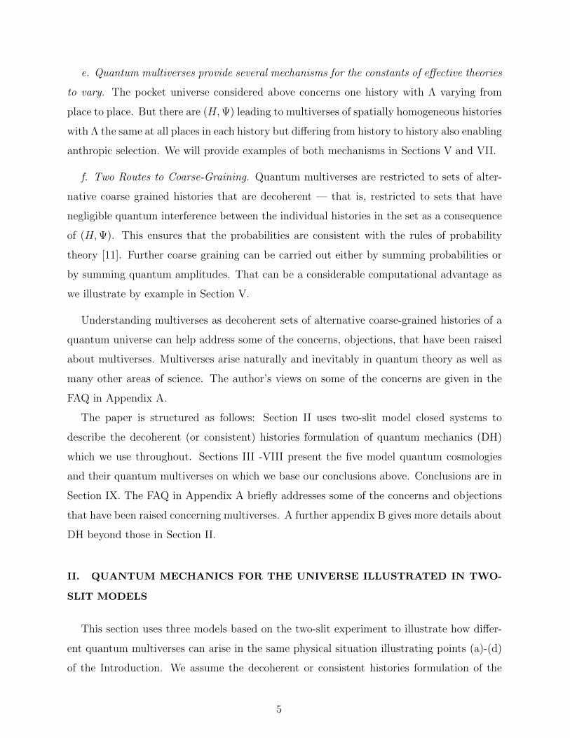
e. Quantum multiverses provide several mechanisms for the constants of effective theories

to vary. The pocket universe considered above concerns one history with Λ varying from

place to place. But there are (H,Ψ) leading to multiverses of spatially homogeneous histories

with Λ the same at all places in each history but differing from history to history also enabling

anthropic selection. We will provide examples of both mechanisms in Sections V and VII.

f. Two Routes to Coarse-Graining. Quantum multiverses are restricted to sets of alter-

native coarse grained histories that are decoherent — that is, restricted to sets that have

negligible quantum interference between the individual histories in the set as a consequence

of (H,Ψ). This ensures that the probabilities are consistent with the rules of probability

theory [11]. Further coarse graining can be carried out either by summing probabilities or

by summing quantum amplitudes. That can be a considerable computational advantage as

we illustrate by example in Section V.

Understanding multiverses as decoherent sets of alternative coarse-grained histories of a

quantum universe can help address some of the concerns, objections, that have been raised

about multiverses. Multiverses arise naturally and inevitably in quantum theory as well as

many other areas of science. The author’s views on some of the concerns are given in the

FAQ in Appendix A.

The paper is structured as follows: Section II uses two-slit model closed systems to

describe the decoherent (or consistent) histories formulation of quantum mechanics (DH)

which we use throughout. Sections III -VIII present the five model quantum cosmologies

and their quantum multiverses on which we base our conclusions above. Conclusions are in

Section IX. The FAQ in Appendix A briefly addresses some of the concerns and objections

that have been raised concerning multiverses. A further appendix B gives more details about

DH beyond those in Section II.

II. QUANTUM MECHANICS FOR THE UNIVERSE ILLUSTRATED IN TWO-

SLIT MODELS

This section uses three models based on the two-slit experiment to illustrate how differ-

ent quantum multiverses can arise in the same physical situation illustrating points (a)-(d)

of the Introduction. We assume the decoherent or consistent histories formulation of the

5

quantum mechanics of a closed system such as the universe4. Decoherent histories quantum

theory (DH) is logically consistent, consistent with experiment as far as is known, consistent

with the rest of modern physics such as special relativity and quantum field theory, general

enough for histories, general enough for cosmology, and generalizable to include semiclassical

quantum gravity. Copenhagen quantum mechanics is contained within DH as an approx-

imation appropriate for measurement situations. DH can be thought of as an extension,

clarification, and, to some extent, a completion of the program started by Everett [13]. DH

may not be the only formulation of quantum mechanics with these properties but it is the

only one we have at present.

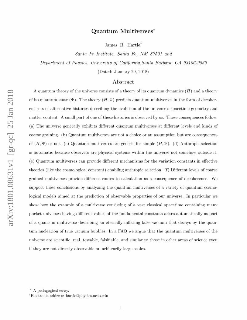
The basic ideas of DH that will be needed in this paper can be introduced with three

model two-slit situations each in a closed box — three very simple model universes. We will

illustrate a variety of quantum multiverses with these simple situations. The three models

are illustrated in Figure 1. We discuss these informally with a minimum of equations in this

section. The same discussion with more equations can be found in Appendix B.

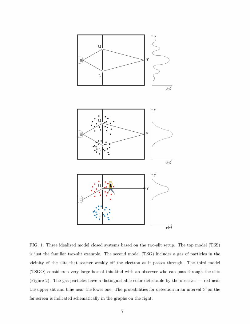
TSS: In the first model the box contains an electron gun at left that emits an electron

which moves through a screen with two slits S = (U,L) to arrive at a further screen at right

in one of a set of position intervals Y = (1, 2, 3 · · · ). We call this the “simple two-slit model

(TSS)”.

TSG: In the second model, in addition to the the contents of TSS, there is a gas of particles

near the slits. These scatter off the electron weakly enough not to disturb its motion but

strongly enough to carry away phases. The gas particles constitute an environment for the

electron in the sense discussed by [14–16] and many others. We call this the “two-slit with

gas model (TSG)”.

TSGO: In the third model the gas particles in TSG have an observable color — red near

the upper slit and blue near the lower one. The electron is replaced by an observer moving

through the slits — so the box must be very large! In these respects the model is closer to

the real universe where observers are physical systems within the universe and not somehow

outside. We call this the “two-slit with gas and observer model (TSGO)”. Figure 2 is a more

evocative image of this.

We stress that in all three examples the boxes are closed — like the universe. There

4 For classic references see [11]. For a tutorial see, e.g. [12].

6

U

y

p(y)

L

Y

U

y

p(y)

L

Y

U

y

p(y)

L

Y

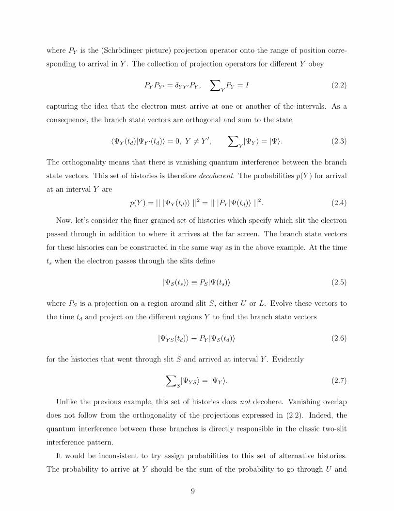
FIG. 1: Three idealized model closed systems based on the two-slit setup. The top model (TSS)

is just the familiar two-slit example. The second model (TSG) includes a gas of particles in the

vicinity of the slits that scatter weakly off the electron as it passes through. The third model

(TSGO) considers a very large box of this kind with an observer who can pass through the slits

(Figure 2). The gas particles have a distinguishable color detectable by the observer — red near

the upper slit and blue near the lower one. The probabilities for detection in an interval Y on the

far screen is indicated schematically in the graphs on the right.

7

are no observers outside the box looking at the inside, or measuring what goes on there, or

otherwise meddling with the inside. Any observers are physical systems within a box as in

the TSGO model.

The inputs to the prediction of quantum multiverses are the box’s Hamiltonian H and its

quantum state |Ψ(t)〉. The latter is a function of time in the Schrodinger picture in which

we work. The state can be defined by specifying the a wave function of the electron at the

initial time when it leaves the gun. This state evolves to later times by the Schrodinger

equation as electron moves through the box. Starting in this way branch state vectors can

be constructed for the individual members of sets of alternative histories of the the electron’s

motion through the box. The set is decoherent when all the branches are approximately

mutually orthogonal. Probabilities for histories are then the norms of the branch state

vectors. The computation of these will be described qualitatively in this section; more

mathematical details are described in Appendix B. We move back and forth between wave

functions like (B1) and bras and kets like |Ψ(t)〉 as convenient.

A. Simple Two Slit Model (TSS)

Two sets of coarse-grained histories are readily identified. There is the set of alternative

histories defined by which position interval Y the electron arrives at the screen at time td. A

finer grained set of histories is defined by also specifying the slit S that the electron passes

through on the way to Y . An even finer-grained set of alternative histories would specify the

path the electron takes at each moment of time, but just the first two sets will be sufficient

to illustrate what we need.

Do these two sets of histories define different quantum multiverses that TSS exhibits?

Not yet! We still have to check that the sets are decoherent, that is, that the squares of

their amplitudes that give probabilities that are consistent with the usual rules of probability

theory.

A branch state vector corresponds to each of the histories in a set of alternative ones.

Consider, for example, the set where the histories are labeled only by the different values Y

at the screen. The branch state vectors for this set are

|ΨY (td)〉 ≡ PY |Ψ(td)〉, Y = 1, 2, 3, · · · (2.1)

8

where PY is the (Schrodinger picture) projection operator onto the range of position corre-

sponding to arrival in Y . The collection of projection operators for different Y obey

PY PY ′ = δY Y ′PY ,∑

YPY = I (2.2)

capturing the idea that the electron must arrive at one or another of the intervals. As a

consequence, the branch state vectors are orthogonal and sum to the state

〈ΨY (td)|ΨY ′(td)〉 = 0, Y 6= Y ′,∑

Y|ΨY 〉 = |Ψ〉. (2.3)

The orthogonality means that there is vanishing quantum interference between the branch

state vectors. This set of histories is therefore decoherent. The probabilities p(Y ) for arrival

at an interval Y are

p(Y ) = || |ΨY (td)〉 ||2 = || |PY |Ψ(td)〉 ||2. (2.4)

Now, let’s consider the finer grained set of histories which specify which slit the electron

passed through in addition to where it arrives at the far screen. The branch state vectors

for these histories can be constructed in the same way as in the above example. At the time

ts when the electron passes through the slits define

|ΨS(ts)〉 ≡ PS|Ψ(ts)〉 (2.5)

where PS is a projection on a region around slit S, either U or L. Evolve these vectors to

the time td and project on the different regions Y to find the branch state vectors

|ΨY S(td)〉 ≡ PY |ΨS(td)〉 (2.6)

for the histories that went through slit S and arrived at interval Y . Evidently∑S|ΨY S〉 = |ΨY 〉. (2.7)

Unlike the previous example, this set of histories does not decohere. Vanishing overlap

does not follow from the orthogonality of the projections expressed in (2.2). Indeed, the

quantum interference between these branches is directly responsible in the classic two-slit

interference pattern.

It would be inconsistent to try assign probabilities to this set of alternative histories.

The probability to arrive at Y should be the sum of the probability to go through U and

9

arrive at Y and the probability to go through L and arrive at Y . But in quantum mechanics

probabilities are squares of amplitudes and

|| |ΨY 〉||2 = || |ΨY U(td)〉+ |ΨY L(td)〉 ||2 6= || |ΨY U(td)〉 ||2 + || |ΨY L(td)〉 ||2 (2.8)

because of quantum interference.

Thus, the finer-grained set following both Y and S does not give us a further quantum

multiverse because it is not decoherent. In Copenhagen quantum mechanics we would

have said that there are no probabilities for S because probabilities are assigned only to the

outcomes of measurements and we didn’t measure which slit the electron went through. The

Copenhagen approximation is consistent with DH because measured alternatives decohere

(e.g. [17, 18]). But decoherence is a more general, more observer independent criterion for

assigning probabilities that apply to histories of the universe as a whole.

B. Two-slit Model with Gas (TSG):

TSG differs from TSS only in the presence of the weakly interacting gas. The weak

interaction with the gas means the set of histories coarse grained only by different values

Y will decohere and and have nearly identical probabilities to the same set of histories in

TSS. But there will be a significant difference between TSS and TSG for a set of histories

that follows S as well as Y . The branch state vectors (2.6) must now include the degrees of

freedom of the scattering particles. Scattering from the upper slit leads to as different state

of the gas than scattering from the lower slit. If enough gas particles scatter these states

can be nearly orthogonal leading decoherence of the set of histories that follows both S and

Y . This argument is given more quantitatively in Appendix B

Thus for TSG we have exhibited two multiverses at different levels of coarse graining.

The first one (just Y ) is a coarse graining of the second (Y, S). The first ignores the gas,

the second follows it.

Which of these two multiverses really describes the box model universe? Both of them.

They are descriptions of the same system at different levels of coarse graining. Which of the

two descriptions should be used to calculate the probability p(Y ) that the electron arrives

at interval Y on the far screen? Either of them because they both supply probabilities that

are consistent with one another.

10

Useful descriptions of a physical system at different levels of coarse graining are familiar

from statistical mechanics. A fine-grained description of a box of gas would specify the

position and momentum of every particle in the box. A much coarser but more useful

description specifies only the total energy, angular momentum, and number of particles in

the box. These differ greatly in utility and computational complexity.

This model illustrates two of the conclusions in the Introduction. First (a) even for simple

systems like TSG the theory (H,Ψ) will predict many different multiverses at different levels

and kinds of coarse graining. The two illustrated here are compatible in the sense that one

is a coarse graining of the other. But that does not have to be the case. The universe may

exhibit incompatible coarse grainings for which there is no finer grained decoherent set of

which they are both coarse grainings (think position and momentum.) (See, e.g [17]).

The model also illustrates conclusion (b) in the Introduction that multiverses are not a

choice or an assumption. The possible multiverses follow from the the basic theory of the

two-slit experiment. You can choose one multiverse or another to calculate with, but you

can’t choose whether the theory exhibits them or not.

The model also illustrates conclusion (f) in the Introduction. The equivalence of coarse

graining by summing quantum amplitudes with coarse graining by summing probabilities is

one way of stating the consistency between different sets that is a consequence of decoherence.

The TSG model gives a specific example. Suppose that we are interested in the probability

p(Y ) that the electron arrives in interval Y . This can be written in two different ways as a

consequence of decoherence

p(Y ) =∑

Sp(Y, S) =

∑S|| |ΨY S〉||2, (sum probabilities) (2.9a)

p(Y ) = || |ΨY 〉||2 = ||∑

S|ΨY S〉||2 (sum amplitudes) (2.9b)

The first is coarse graining by summing probabilities for histories, the second is coarse

graining by summing amplitudes for histories. Which of these formulae should be used to

calculate p(Y )? It doesn’t make any difference, they both give the same answer because the

probabilities are consistent as a consequence of decoherence. Summing amplitudes is usually

easier than summing probabilities because less computation is involved. This is a triviality

in this example but, as we will illustrate in Section VI, this simplicity is a considerable

advantage in physically complex situations.

11

C. Two-slit Model with Gas and Observer (TSGO)

1. Third and First Person Probabilities

TSS and TSG have quantum multiverses that provide probabilities for which of a set of

alternative histories happens in the box whether or not they are subject to the attention of

observers. These probabilities for which history happens are called third person probabilities

and are derivable just from (H,Ψ). As observers of the universe we are interested in the

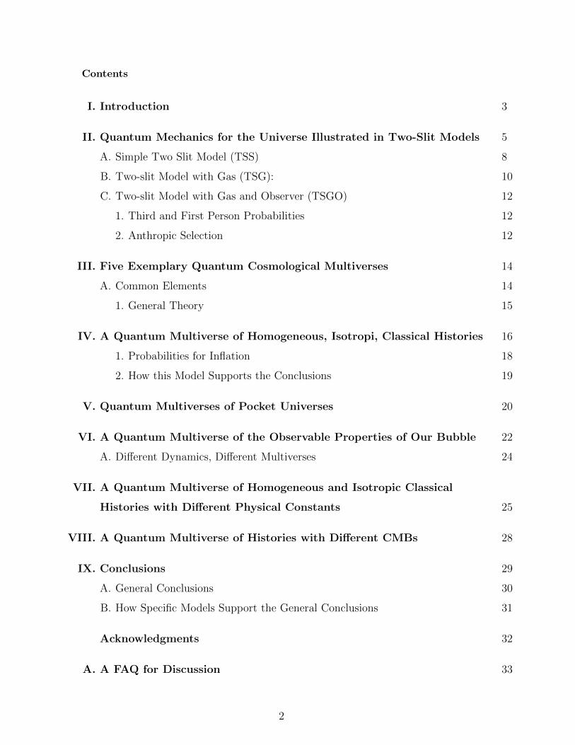
probabilities for what we observe. To discuss this TSGO includes a model observer as a

physical system within the box and assumes that the gas particles of TSS have a detectable

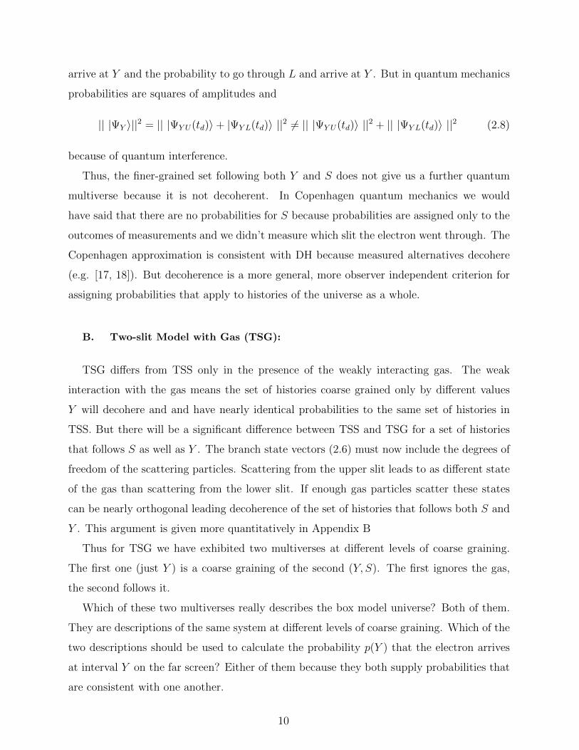
color — red near the upper slit and blue near the lower slit. See Figure 2.

An observer moves through the two-slit setup (which must be very large) equipped with

a detector that can measure the color of any gas detected. If the detector registers ‘red’ the

observer knows that she is passing through the upper slit. Given this data red, or what is the

same thing, given that she passed through U , what does she predict for the probability that

she will arrive in the interval Y at the further screen. This is an example of a first person

probability — a probability for the result of an observation 5. First person probabilities are

third person probabilities for what happens conditioned on data that describes observational

situation. In this case, the observer’s data is that she passed through the upper slit U . The

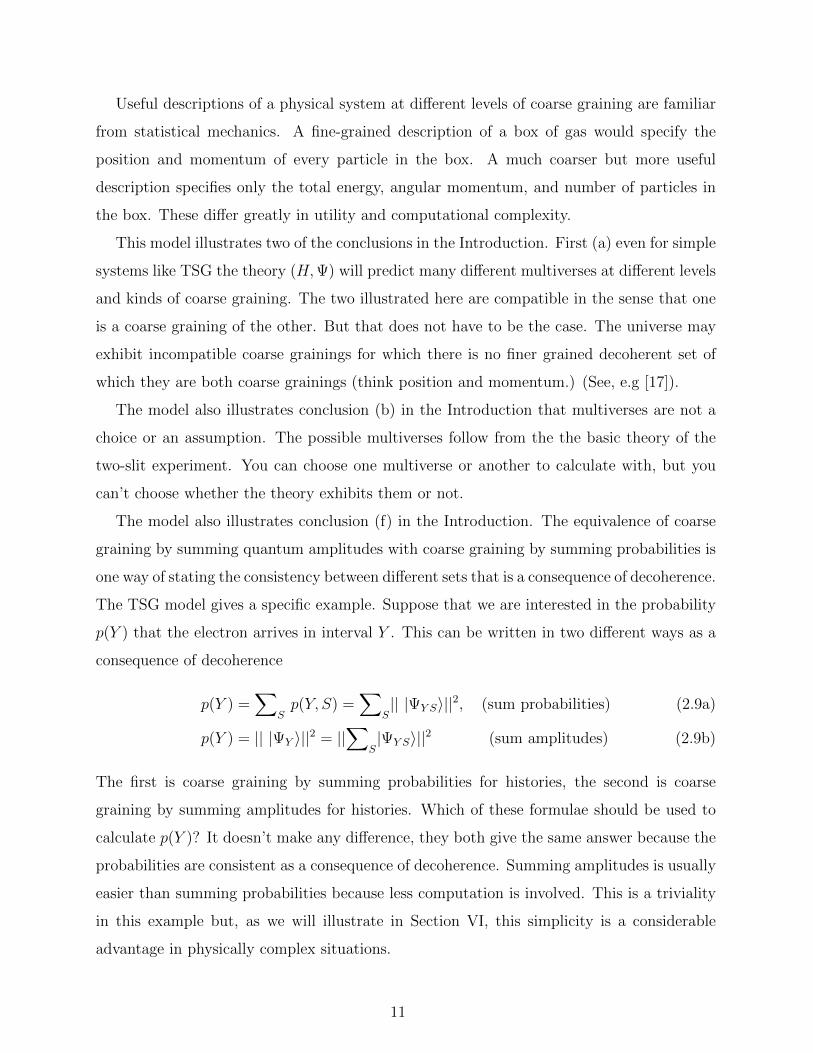
first person probability that she observes Y at the further screen is then

p(1p)(Y ) = p(Y |U) =p(Y, U)

p(U)=||PY |ΨU(td)〉||2

|| |ΨU(td)〉||2. (2.10)

The distribution is illustrated in bottom image in Figure 1. As should be clear from com-

paring that with the figure immediately above what is most probable to occur is not the

most probable to be observed.

2. Anthropic Selection

Up to now we have tacitly assumed in TSGO that a live observer (us) exists (E) in the

box for all times in all cases. Since an observer is a physical system within the box there is a

5 In other work we have called first person probabilities ‘bottom up probabilities’ and third person proba-

bilities ‘top-down probabilities’ [19] and especially [20]

12

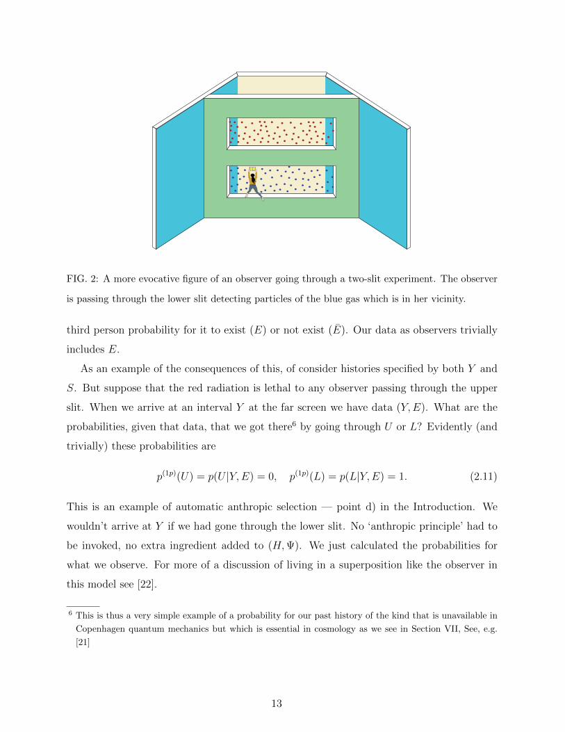
FIG. 2: A more evocative figure of an observer going through a two-slit experiment. The observer

is passing through the lower slit detecting particles of the blue gas which is in her vicinity.

third person probability for it to exist (E) or not exist (E). Our data as observers trivially

includes E.

As an example of the consequences of this, of consider histories specified by both Y and

S. But suppose that the red radiation is lethal to any observer passing through the upper

slit. When we arrive at an interval Y at the far screen we have data (Y,E). What are the

probabilities, given that data, that we got there6 by going through U or L? Evidently (and

trivially) these probabilities are

p(1p)(U) = p(U |Y,E) = 0, p(1p)(L) = p(L|Y,E) = 1. (2.11)

This is an example of automatic anthropic selection — point d) in the Introduction. We

wouldn’t arrive at Y if we had gone through the lower slit. No ‘anthropic principle’ had to

be invoked, no extra ingredient added to (H,Ψ). We just calculated the probabilities for

what we observe. For more of a discussion of living in a superposition like the observer in

this model see [22].

6 This is thus a very simple example of a probability for our past history of the kind that is unavailable in

Copenhagen quantum mechanics but which is essential in cosmology as we see in Section VII, See, e.g.

[21]

13

III. FIVE EXEMPLARY QUANTUM COSMOLOGICAL MULTIVERSES

The most striking observable feature of our quantum universe is its classical spacetime.

At some level and kind of coarse graining this extends over the whole of the visible universe

from near the big bang to the distant future. What is the origin of this realm of classi-

cal predictability in a quantum theory characterized fundamentally by indeterminacy and

distributed probabilities? How does it emerge from theory (H,Ψ) that includes quantum

gravity where spacetime geometry is generally fluctuating and without definite value? Many

of our cosmological observations are of properties of the universe’s classical spacetime and

its contents — the expansion, the approximate homogeneity and isotropy on large scales,

the distribution of galaxies, the CMB, the value of the cosmological constant, etc.

Classical behavior is not a given in a quantum universe. It is a matter of quantum

probabilities. A quantum system behaves classically when, in a suitable quantum multiverse

of alternative histories, the probabilities are high for those histories exhibiting correlations in

time governed by deterministic laws. The relevant probabilities follow from (H,Ψ). Classical

spacetime emerges when the probabilities are high for spacetime geometries correlated in

time by the Einstein equation7.

Subsequent sections III through VIII exhibit five models of a quantum multiverse of

classical spacetimes that illustrate conclusions (a)-(f) of the Introduction. The models are

based on the author’s joint work with Stephen Hawking and Thomas Hertog (mainly [3, 8–

10]). We do not pretend to present these models in the depth and precision that they are

discussed in those papers. Rather, we present a qualitative and intuitive descriptions of the

models.

A. Common Elements

The five models have the following elements in common:

7 The rest of the domain of applicability of classical physics constituting the quasiclassical realm of every

day experience is a consequence of this [23].

14

1. General Theory

Semiclassical Quantum Gravity:— Quantum multiverses of the universe necessarily in-

clude alternative histories of cosmological spacetime geometry and therefore involve quantum

gravity at some approximate level. Phenomena like the emergence of classical spacetime from

the quantum big bang, the generation of large scale structure from quantum fluctuations

away from homogeneity and isotropy, the nucleation of bubbles of true vacuum in a false

vacuum, and eternal inflation are all fundamentally quantum spacetime phenomena. We

discuss these treating quantum gravity in semiclassical approximation.

Quantum State: For the quantum state Ψ we adopt the no-boundary wave function of

the universe (NBWF) in its semiclassical approximation [7].

Dynamics: For a theory of dynamics (H) we assume Einstein gravity coupled to a single

homogeneous scalar field φ(t) moving in a potential V (φ). Different models have different

V (φ)

Coarse Graining: The theory (H,Ψ) predicts different quantum multiverses defined by

coarse grainings that follow different variables on very different scales. Coarse grainings

relevant for laboratory experiment follow the outcomes of the experiment and ignore cosmo-

logical scale features of the universe if these do not affect the outcomes. Coarse grainings

relevant for cosmology follow the large scale features of the universe and ignore small scale

fluctuations like planets, biota, human observers, and their laboratory experiments whose

presence or absence has little effect on the large scale behavior of the universe.

A Model of Observers and Observation: By itself, the theory (H,Ψ) predicts third person

probabilities for which of a set of alternative histories of classical spacetime geometries and

the matter within happens. First person probabilities for our observations are third person

probabilities for what happened conditioned on the data D describing our observational

situation. TSGO provided a very simple example of this leading to (2.10) and(2.11). There,

the data D was that an observer existed, E. Naturally probabilities for the results of her

observations were conditioned in E.

As observers of the universe we, and the apparatus we use, are quantum physical systems

within it not somehow outside it. Our observations of the universe are limited to a spatial

volume of rough size c/(Hubble constant) ∼ 4000Mpc at the present time — our Hubble

volume. This is just one Hubble volume in a universe that may have a great many similar

15

volumes. We have only a very, very small probability that we denote by pE(D) to have

evolved in any Hubble volume. Incorporating, as it does, the probabilities for accidents of

biological evolution, the probability pE(D) is a very, very, very small number much beyond

the ability of present day physics to compute. This is a very crude model of an observing

situation, but still better than many treatments where the evolution of observing systems

in the universe is not considered at all.8

Despite the small value of pE(D) there can be a significant probability that in a very

large universe the data D is replicated in many Hubbble volumes. First person probabilities

for our observations are third person probabilities for what happened conditioned on the

existence of at least one instance of our observational situation — our instance. That’s all

we know for sure about instances of D. We abbreviate (at least one instance of D) by D≥1.

TSGO provided a very simple example of this leading to (2.10) and(2.11).

The bottom line is that first person probabilities for an observable feature of the universe

O are third person probabilities for O to happen from (H,Ψ) conditioned on the existence

of at least one instance of our observational situation D, viz

p(1p)(O) ≡ p(O|D≥1) (3.1)

We describe how to calculate this in the various models beginning with the one in the

next section.

IV. A QUANTUM MULTIVERSE OF HOMOGENEOUS, ISOTROPI, CLASSI-

CAL HISTORIES

This is a very simple model that illustrates how a quantum multiverse of classical space-

time geometries emerges from (H,Ψ).

The model assumes a minisuperspace based on homogeneous, isotropic, spatially closed

spacetime geometries with metrics of the form

ds2 = −dt2 + a2(t)dΩ23. (4.1)

Here, a(t) is the scale factor and dΩ23 is the metric on a unit round 3-sphere.

8 For detail on observers, observations 1st and 3rd person probabilities and what’s included in D etc see

e.g.[19, 24].

16

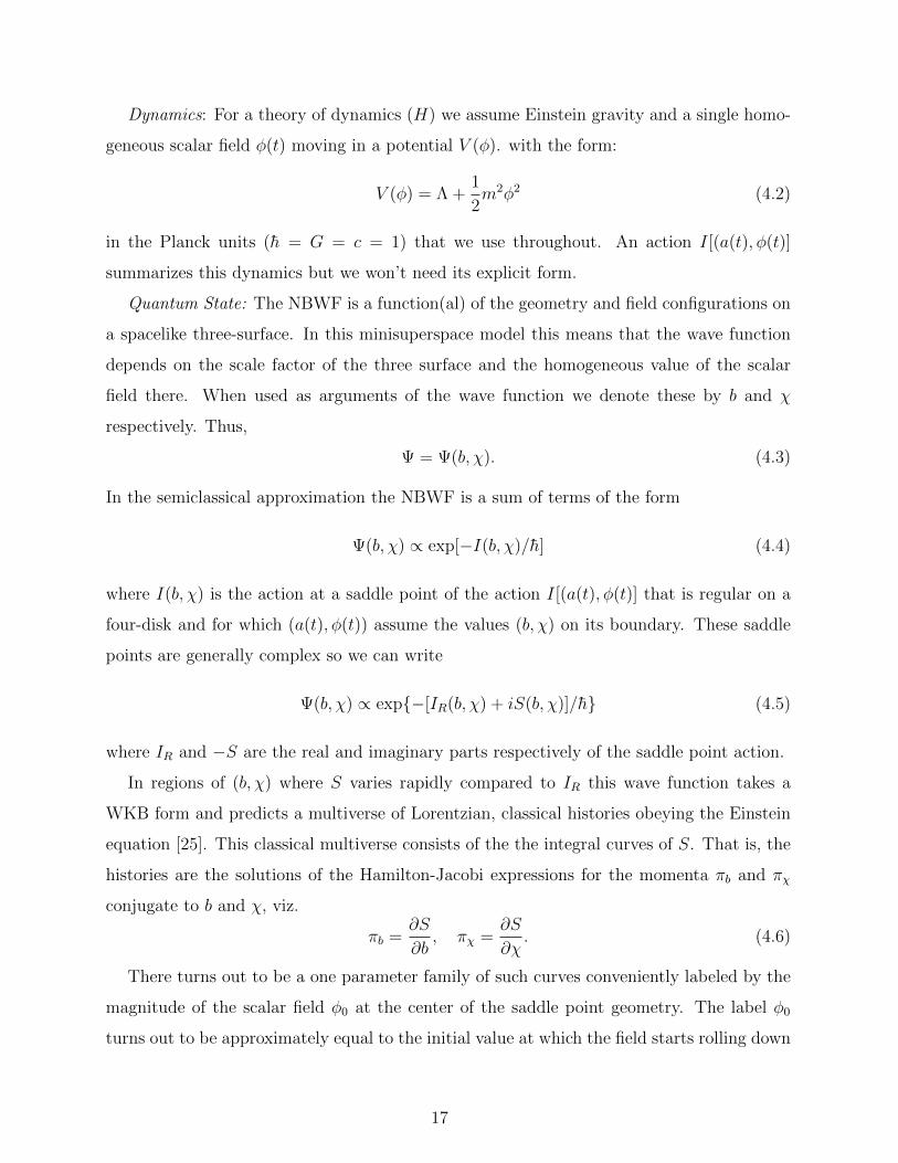
Dynamics: For a theory of dynamics (H) we assume Einstein gravity and a single homo-

geneous scalar field φ(t) moving in a potential V (φ). with the form:

V (φ) = Λ +1

2m2φ2 (4.2)

in the Planck units (h = G = c = 1) that we use throughout. An action I[(a(t), φ(t)]

summarizes this dynamics but we won’t need its explicit form.

Quantum State: The NBWF is a function(al) of the geometry and field configurations on

a spacelike three-surface. In this minisuperspace model this means that the wave function

depends on the scale factor of the three surface and the homogeneous value of the scalar

field there. When used as arguments of the wave function we denote these by b and χ

respectively. Thus,

Ψ = Ψ(b, χ). (4.3)

In the semiclassical approximation the NBWF is a sum of terms of the form

Ψ(b, χ) ∝ exp[−I(b, χ)/h] (4.4)

where I(b, χ) is the action at a saddle point of the action I[(a(t), φ(t)] that is regular on a

four-disk and for which (a(t), φ(t)) assume the values (b, χ) on its boundary. These saddle

points are generally complex so we can write

Ψ(b, χ) ∝ exp−[IR(b, χ) + iS(b, χ)]/h (4.5)

where IR and −S are the real and imaginary parts respectively of the saddle point action.

In regions of (b, χ) where S varies rapidly compared to IR this wave function takes a

WKB form and predicts a multiverse of Lorentzian, classical histories obeying the Einstein

equation [25]. This classical multiverse consists of the the integral curves of S. That is, the

histories are the solutions of the Hamilton-Jacobi expressions for the momenta πb and πχ

conjugate to b and χ, viz.

πb =∂S

∂b, πχ =

∂S

∂χ. (4.6)

There turns out to be a one parameter family of such curves conveniently labeled by the

magnitude of the scalar field φ0 at the center of the saddle point geometry. The label φ0

turns out to be approximately equal to the initial value at which the field starts rolling down

17

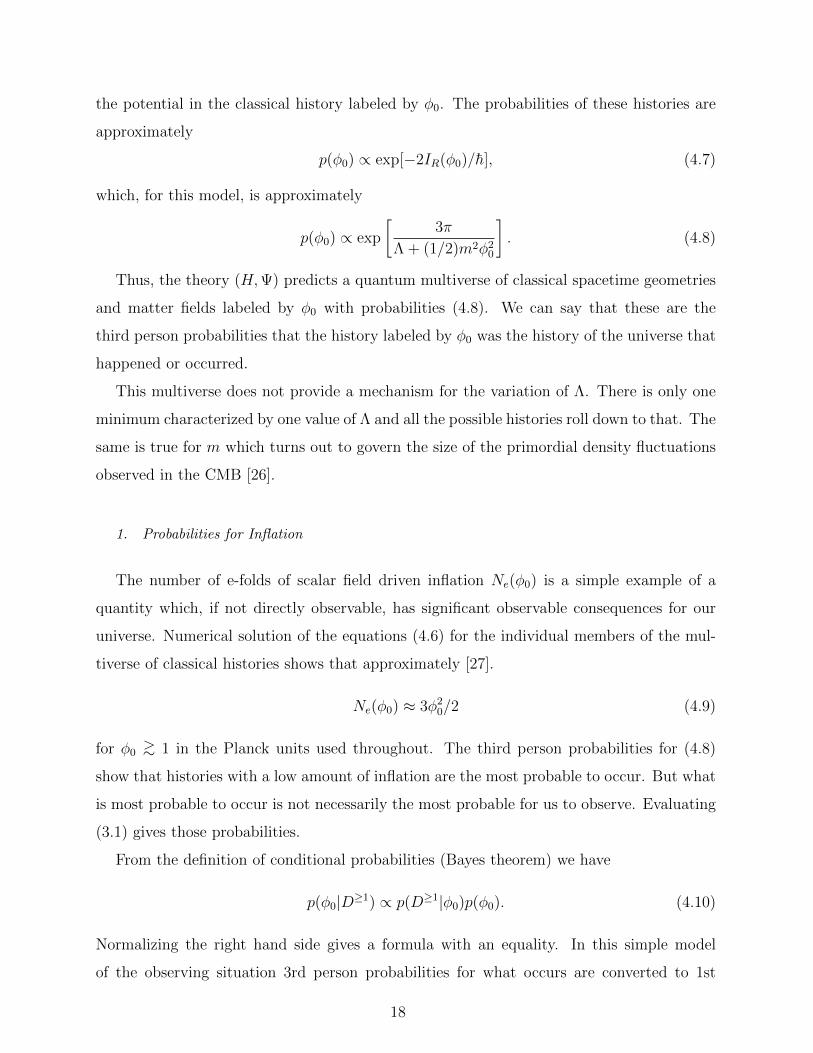
the potential in the classical history labeled by φ0. The probabilities of these histories are

approximately

p(φ0) ∝ exp[−2IR(φ0)/h], (4.7)

which, for this model, is approximately

p(φ0) ∝ exp

[3π

Λ + (1/2)m2φ20

]. (4.8)

Thus, the theory (H,Ψ) predicts a quantum multiverse of classical spacetime geometries

and matter fields labeled by φ0 with probabilities (4.8). We can say that these are the

third person probabilities that the history labeled by φ0 was the history of the universe that

happened or occurred.

This multiverse does not provide a mechanism for the variation of Λ. There is only one

minimum characterized by one value of Λ and all the possible histories roll down to that. The

same is true for m which turns out to govern the size of the primordial density fluctuations

observed in the CMB [26].

1. Probabilities for Inflation

The number of e-folds of scalar field driven inflation Ne(φ0) is a simple example of a

quantity which, if not directly observable, has significant observable consequences for our

universe. Numerical solution of the equations (4.6) for the individual members of the mul-

tiverse of classical histories shows that approximately [27].

Ne(φ0) ≈ 3φ20/2 (4.9)

for φ0>∼ 1 in the Planck units used throughout. The third person probabilities for (4.8)

show that histories with a low amount of inflation are the most probable to occur. But what

is most probable to occur is not necessarily the most probable for us to observe. Evaluating

(3.1) gives those probabilities.

From the definition of conditional probabilities (Bayes theorem) we have

p(φ0|D≥1) ∝ p(D≥1|φ0)p(φ0). (4.10)

Normalizing the right hand side gives a formula with an equality. In this simple model

of the observing situation 3rd person probabilities for what occurs are converted to 1st

18

person probabilities for what is observed by multiplying by the factor p(D≥1|φ0) called the

‘top-down’ factor and then renormalizing.

The probability that there is at least one instance of our observational situation some-

where in the universe, p(D≥1|φ0) is bigger in a larger universe where there are more Hubble

volumes for an instance of D to have evolved than it is in a smaller universe where there are

fewer Hubble volumes. This turns out to mean that we are more likely to observe universes

with more inflation [28].

We can understand this result more quantitatively with a little model where p(D≥1|φ0)

can be explicitly evaluated. Suppose that our data D locate us somewhere on a homoge-

neous isotropic spacelike surface with Nh(φ0) Hubble volumes in each classical history. The

probability p(D≥1|φ0) is one minus the probability that there are no instances of D on the

surface. This in turn is the product of the probabilities 1−pE(D) that there are no instances

of D in any particular Hubble volume on the surface. The result is the formula:

p(D≥1|φ0) = 1− [1− pE(D)]Nh(φ0). (4.11)

Eq. (4.11) is an explicit formula for the ‘top-down factor’ that converts 3rd person probabil-

ities to first person ones as in (4.10). Larger number of Hubble volumes Nh make this factor

larger and closer and closer to 1. However small pE(D) is, in a sufficiently large universe the

probability is 1 that an instance of D occurs somewhere. When Nh 1/pE(D) first person

probabilities are equal to third person ones.

First person probabilities thus favor larger universes, larger φ0, with more e-folds for

inflation (4.9). In the quantum multiverse considered in this section significant inflation is

anthropically selected to be observed.

2. How this Model Supports the Conclusions

The main contribution of this model to our exposition is to illustrate in a simple way how

quantum multiverses of classical histories (including spacetime geometry) are predicted by

(H,Ψ). We will assume this for subsequent models. But the model does illustrate points (b)

and (c) of the Introduction, namely that quantum multiverses are a consequence of (H,Ψ)

and typically consist of many different histories not just one.

19

A

V

B

ΛB

φ

F

φBφA

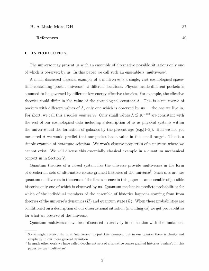
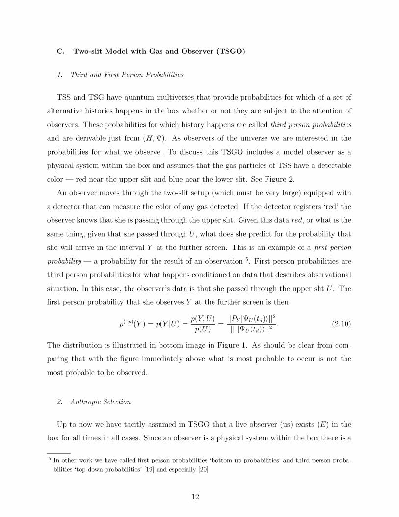
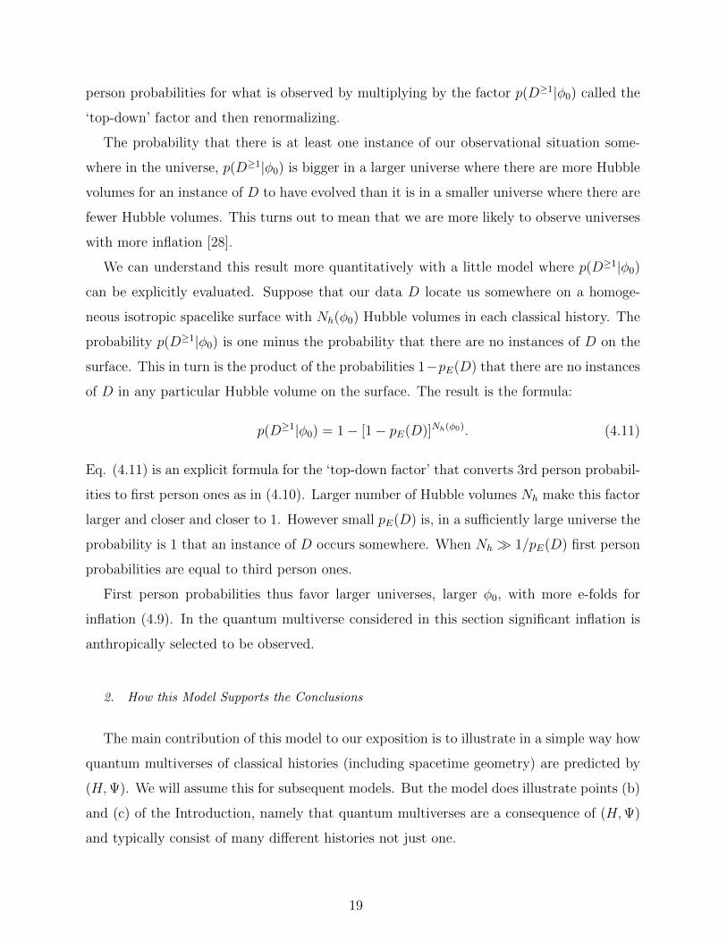
FIG. 3: A potential for the scalar field with one false vacuum F and two true vacua A and B. The

false vacuum is separated from either true vacua by potential barriers and relatively flat patches

where the conditions for slow roll inflation are satisfied. The different shape of the barriers and of

the potential in the two slow roll regimes leading to the true vacua results in different false vacuum

decay rates and different predictions for CMB related observables in universes ending up in A or

B.

V. QUANTUM MULTIVERSES OF POCKET UNIVERSES

This section shows how pocket multiverses mentioned in the Introduction arise at vari-

ous levels of coarse graining from the NBWF (Ψ) and a dynamical theory (H) based on a

particular potential V (φ) like the one in Figure 3. This potential has three minima (vacua)

— two true vacua A and B and one false vacuum F . We can say that the potential de-

fines a landscape of vacua although there are only three here. As described in Section IV,

(H,Ψ) predicts a one parameter ensemble of classical histories labeled by the value at which

they start to roll down.

The classical history that starts to roll down at F in Figure 3 is a universe that inflates

with an effective cosmological constant 3π/V (0). Classically this inflation is eternal — goes

on forever. But quantum mechanically regions of spacetime can tunnel through the barriers

20

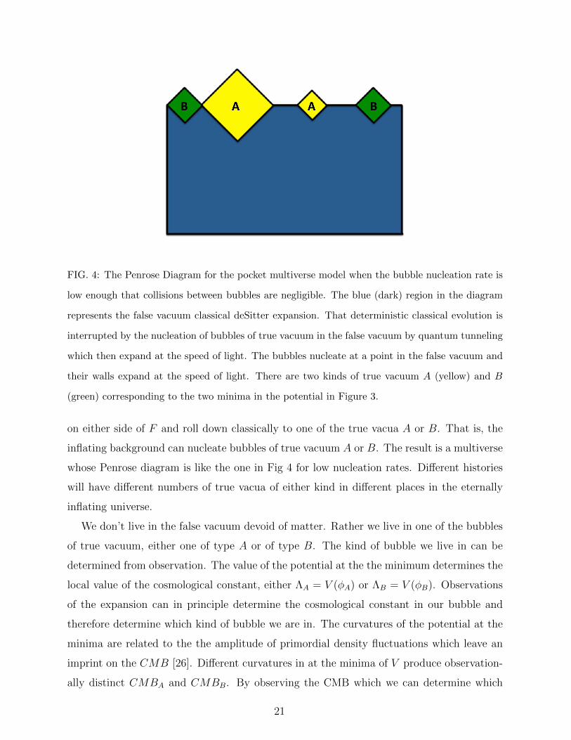
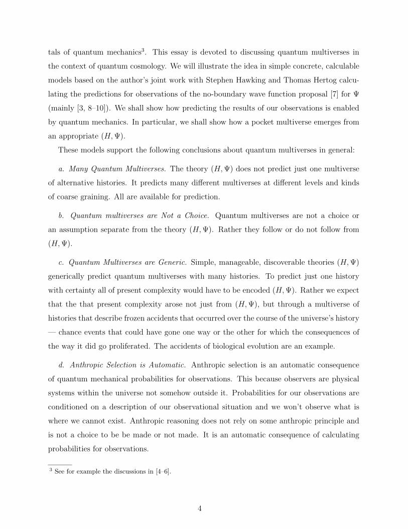
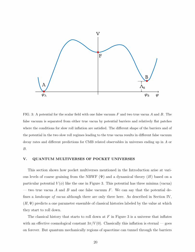
FIG. 4: The Penrose Diagram for the pocket multiverse model when the bubble nucleation rate is

low enough that collisions between bubbles are negligible. The blue (dark) region in the diagram

represents the false vacuum classical deSitter expansion. That deterministic classical evolution is

interrupted by the nucleation of bubbles of true vacuum in the false vacuum by quantum tunneling

which then expand at the speed of light. The bubbles nucleate at a point in the false vacuum and

their walls expand at the speed of light. There are two kinds of true vacuum A (yellow) and B

(green) corresponding to the two minima in the potential in Figure 3.

on either side of F and roll down classically to one of the true vacua A or B. That is, the

inflating background can nucleate bubbles of true vacuum A or B. The result is a multiverse

whose Penrose diagram is like the one in Fig 4 for low nucleation rates. Different histories

will have different numbers of true vacua of either kind in different places in the eternally

inflating universe.

We don’t live in the false vacuum devoid of matter. Rather we live in one of the bubbles

of true vacuum, either one of type A or of type B. The kind of bubble we live in can be

determined from observation. The value of the potential at the the minimum determines the

local value of the cosmological constant, either ΛA = V (φA) or ΛB = V (φB). Observations

of the expansion can in principle determine the cosmological constant in our bubble and

therefore determine which kind of bubble we are in. The curvatures of the potential at the

minima are related to the the amplitude of primordial density fluctuations which leave an

imprint on the CMB [26]. Different curvatures in at the minima of V produce observation-

ally distinct CMBA and CMBB. By observing the CMB which we can determine which

21

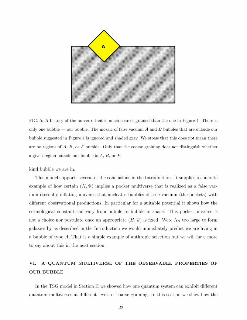
FIG. 5: A history of the universe that is much coarser grained than the one in Figure 4. There is

only one bubble — our bubble. The mosaic of false vacuum A and B bubbles that are outside our

bubble suggested in Figure 4 is ignored and shaded gray. We stress that this does not mean there

are no regions of A, B, or F outside. Only that the coarse graining does not distinguish whether

a given region outside our bubble is A, B, or F .

kind bubble we are in.

This model supports several of the conclusions in the Introduction. It supplies a concrete

example of how certain (H,Ψ) implies a pocket multiverse that is realized as a false vac-

uum eternally inflating universe that nucleates bubbles of true vacuum (the pockets) with

different observational productions, In particular for a suitable potential it shows how the

cosmological constant can vary from bubble to bubble in space. This pocket universe is

not a choice nor postulate once an appropriate (H,Ψ) is fixed. Were ΛB too large to form

galaxies by as described in the Introduction we would immediately predict we are living in

a bubble of type A, That is a simple example of anthropic selection but we will have more

to say about this in the next section.

VI. A QUANTUM MULTIVERSE OF THE OBSERVABLE PROPERTIES OF

OUR BUBBLE

In the TSG model in Section II we showed how one quantum system can exhibit different

quantum multiverses at different levels of coarse graining. In this section we show how the

22

model cosmology defined by the potential like that in Figure 3 can exhibit more than one

quantum multiverse at different levels of coarse graining.

A relatively fine-grained multiverse would consist of histories that describe all possible

configurations of bubble nucleation and non-nucleation at all places and all times. The

history illustrated in Figure 4 is just one example. But there are an infinite number of other

histories at this level of coarse graining in a false vacuum deSitter expansion that extends

to the infinite future.

The (3rd person) probabilities per unit four volume pA and pB for nucleating bubbles of

different kinds were calculated by Coleman and De Lucia (CDL) [29]. The probability per

unit four-volume to remain in the false vacuum is pF = 1−pA−pB. With these probabilities

it is possible to imagine calculating the third person probabilities for an entire set of histories

of different mosaics of volumes of false and true vacua. Some kind of cutoff or ‘measure’

would be required to deal with the infinite volume. Even then it would be a formidable

calculation.

We do not observe entire four-dimensional histories of roiling seas of bubble nucleation

extending to the infinite future. Neither do we know the location of our bubble. First

person probabilities for our observations, say of the CMB, are the probabilities that we

are in a bubble of type A or B at some unknown location in the eternally inflating false

vacuum spacetime. Such probabilities could in principle be calculated by summing the

probabilities for the fine-grained histories over the all the alternative structures outside our

bubble. Quantum mechanics provides a more direct route to the answer: Make predictions

for our observations using a quantum multiverse based on a much coarser grained multiverse

that follows what goes on inside our bubble and ignores everything outside — a multiverse

based on our bubble.

A history in our bubble multiverse is illustrated in Figure 5. Our bubble occupies one

part of the spacetime with (CDL) probabilities pA or pB that it is of type A or B. Since

the coarse-graining doesn’t specify what is going on in the volumes outside our bubble their

contribution to the probability of this coarse-grained history is pA + pB + pF = 1.

Suppose the data D describing our observational situation locate us on the spacelike

reheating surface inside one of these kinds of bubbles. There are an infinite number of

Hubble volumes on these surfaces in both kinds of bubble. The top-down factor (4.11)

connecting 1st and 3rd person probabilities is then unity. 1st person probabilities equal 3rd

23

person probabilities. Thus, the probabilities that we observe A, p(WOA) or B p((WOB)

are

p(WOA) =pA

pA + pB, p(WOB) =

pBpA + pB

(6.1)

It doesn’t matter where in spacetime our bubble is located. CDL probabilities respect the

symmetries of deSitter space and are the same at all locations.

This example illustrates that a quantum system like our universe is not described by only

one quantum multiverse. It is described by many different ones at different levels of coarse

graining within the same theory (H,Ψ) with the same potential in Figure 3. For a given

question it’s generally best to use the coarsest grained description that supplies an answer

to it.

This model supports all of the conclusions (a)-(f) mentioned in the Introduction (a)

Different quantum multiverses follow from (H,Ψ) at different levels and kinds of coarse

graining. (b) They emerged by calculation from (H,Ψ)with the potential in Fig 3. They

were not an assumption beyond assuming (H,Ψ). (c.) The coarse graining following the

alternatives A, B, or F for all volumes in spacetime leads to quantum multiverse with a

truly vast number of histories to compute third person probabilities for. The coarse graining

following only the inside of our bubble and ignoring everything outside has only alternatives

A or B. Either way there is a multiplicity of alternative histories. (d.) Anthropic selection

automatically ruled out an observation of a false vacuum F devoid of matter where we

cannot exist. (f.) The simplicity of coarse graining multiverses by summing amplitudes

rather than summing probabilities.

A. Different Dynamics, Different Multiverses

Our story about pocket universes forming by the decay of an eternally inflating false

vacuum depended crucially on a dynamical theory (H) incorporating something like the po-

tential in Figure 3. This dependence on dynamical theory is illustrated in work by Hawking

and Hertog [30]. They use the no-boundary quantum state (Ψ) together with a dynamics

(H) specified by an effective dual field theory defined on the exit surface of eternal inflation.

This dual field theory provides a description of the transition between the essentially quan-

tum realm of eternal inflation to the ensemble of possible classical universes one of which we

observe. It provides a quantum probabilistic measure on this ensemble that is different from

24

V(φ)

φ

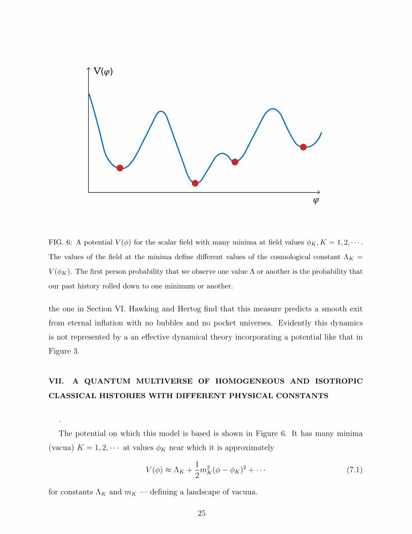
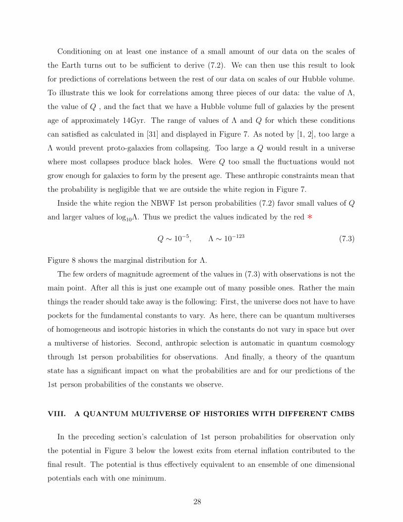
FIG. 6: A potential V (φ) for the scalar field with many minima at field values φK ,K = 1, 2, · · · .

The values of the field at the minima define different values of the cosmological constant ΛK =

V (φK). The first person probability that we observe one value Λ or another is the probability that

our past history rolled down to one minimum or another.

the one in Section VI. Hawking and Hertog find that this measure predicts a smooth exit

from eternal inflation with no bubbles and no pocket universes. Evidently this dynamics

is not represented by a an effective dynamical theory incorporating a potential like that in

Figure 3.

VII. A QUANTUM MULTIVERSE OF HOMOGENEOUS AND ISOTROPIC

CLASSICAL HISTORIES WITH DIFFERENT PHYSICAL CONSTANTS

.

The potential on which this model is based is shown in Figure 6. It has many minima

(vacua) K = 1, 2, · · · at values φK near which it is approximately

V (φ) ≈ ΛK +1

2m2K(φ− φK)2 + · · · (7.1)

for constants ΛK and mK — defining a landscape of vacuua.

25

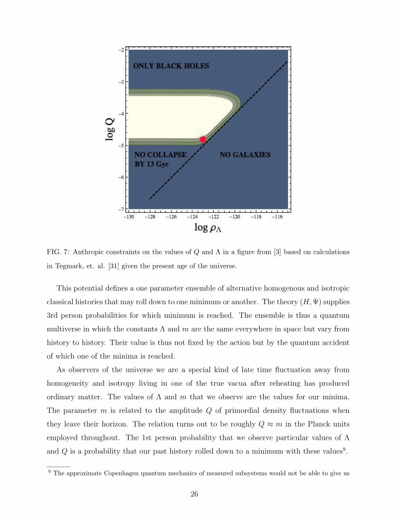
FIG. 7: Anthropic constraints on the values of Q and Λ in a figure from [3] based on calculations

in Tegmark, et. al. [31] given the present age of the universe.

This potential defines a one parameter ensemble of alternative homogenous and isotropic

classical histories that may roll down to one minimum or another. The theory (H,Ψ) supplies

3rd person probabilities for which minimum is reached. The ensemble is thus a quantum

multiverse in which the constants Λ and m are the same everywhere in space but vary from

history to history. Their value is thus not fixed by the action but by the quantum accident

of which one of the minima is reached.

As observers of the universe we are a special kind of late time fluctuation away from

homogeneity and isotropy living in one of the true vacua after reheating has produced

ordinary matter. The values of Λ and m that we observe are the values for our minima.

The parameter m is related to the amplitude Q of primordial density fluctuations when

they leave their horizon. The relation turns out to be roughly Q ≈ m in the Planck units

employed throughout. The 1st person probability that we observe particular values of Λ

and Q is a probability that our past history rolled down to a minimum with these values9.

9 The approximate Copenhagen quantum mechanics of measured subsystems would not be able to give us

26

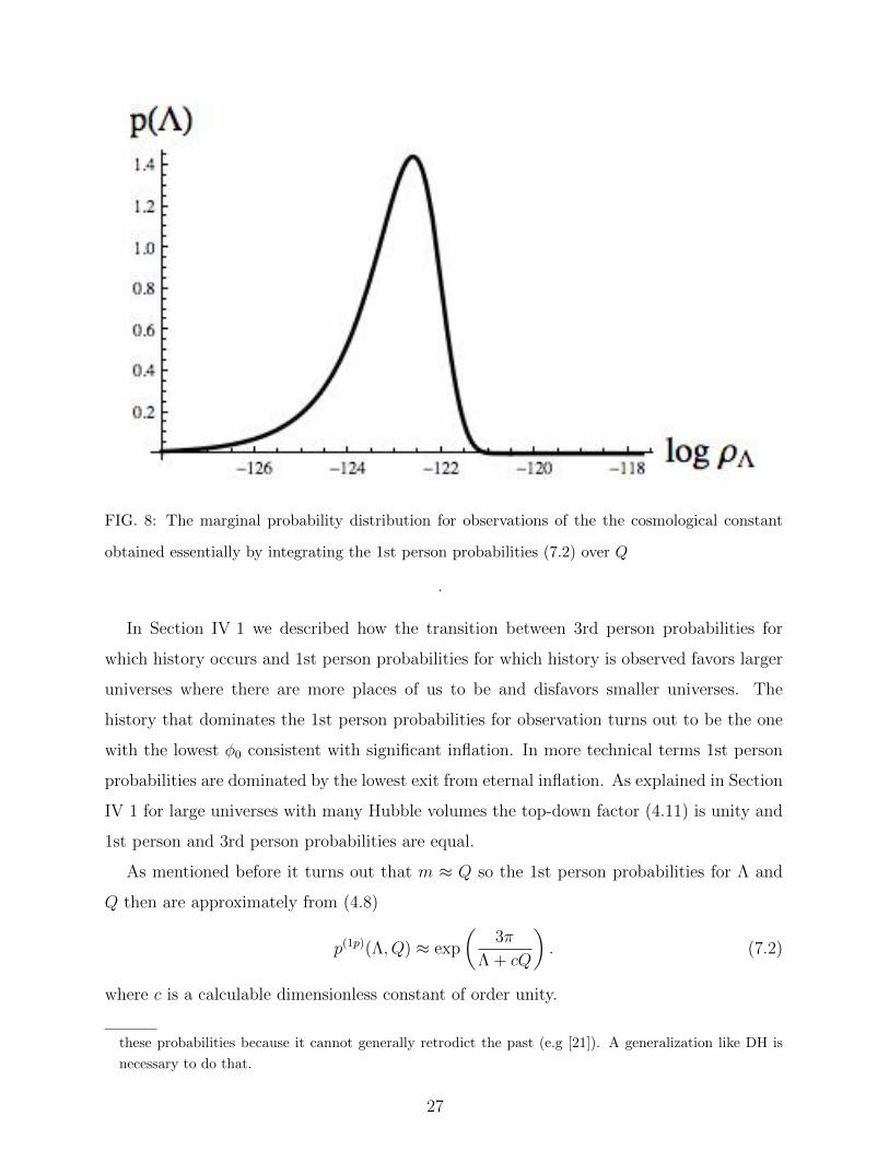
FIG. 8: The marginal probability distribution for observations of the the cosmological constant

obtained essentially by integrating the 1st person probabilities (7.2) over Q

.

In Section IV 1 we described how the transition between 3rd person probabilities for

which history occurs and 1st person probabilities for which history is observed favors larger

universes where there are more places of us to be and disfavors smaller universes. The

history that dominates the 1st person probabilities for observation turns out to be the one

with the lowest φ0 consistent with significant inflation. In more technical terms 1st person

probabilities are dominated by the lowest exit from eternal inflation. As explained in Section

IV 1 for large universes with many Hubble volumes the top-down factor (4.11) is unity and

1st person and 3rd person probabilities are equal.

As mentioned before it turns out that m ≈ Q so the 1st person probabilities for Λ and

Q then are approximately from (4.8)

p(1p)(Λ, Q) ≈ exp

(3π

Λ + cQ

). (7.2)

where c is a calculable dimensionless constant of order unity.

these probabilities because it cannot generally retrodict the past (e.g [21]). A generalization like DH is

necessary to do that.

27

Conditioning on at least one instance of a small amount of our data on the scales of

the Earth turns out to be sufficient to derive (7.2). We can then use this result to look

for predictions of correlations between the rest of our data on scales of our Hubble volume.

To illustrate this we look for correlations among three pieces of our data: the value of Λ,

the value of Q , and the fact that we have a Hubble volume full of galaxies by the present

age of approximately 14Gyr. The range of values of Λ and Q for which these conditions

can satisfied as calculated in [31] and displayed in Figure 7. As noted by [1, 2], too large a

Λ would prevent proto-galaxies from collapsing. Too large a Q would result in a universe

where most collapses produce black holes. Were Q too small the fluctuations would not

grow enough for galaxies to form by the present age. These anthropic constraints mean that

the probability is negligible that we are outside the white region in Figure 7.

Inside the white region the NBWF 1st person probabilities (7.2) favor small values of Q

and larger values of log10Λ. Thus we predict the values indicated by the red ∗

Q ∼ 10−5, Λ ∼ 10−123 (7.3)

Figure 8 shows the marginal distribution for Λ.

The few orders of magnitude agreement of the values in (7.3) with observations is not the

main point. After all this is just one example out of many possible ones. Rather the main

things the reader should take away is the following: First, the universe does not have to have

pockets for the fundamental constants to vary. As here, there can be quantum multiverses

of homogeneous and isotropic histories in which the constants do not vary in space but over

a multiverse of histories. Second, anthropic selection is automatic in quantum cosmology

through 1st person probabilities for observations. And finally, a theory of the quantum

state has a significant impact on what the probabilities are and for our predictions of the

1st person probabilities of the constants we observe.

VIII. A QUANTUM MULTIVERSE OF HISTORIES WITH DIFFERENT CMBS

In the preceding section’s calculation of 1st person probabilities for observation only

the potential in Figure 3 below the lowest exits from eternal inflation contributed to the

final result. The potential is thus effectively equivalent to an ensemble of one dimensional

potentials each with one minimum.

28

String theory has a vast landscape of possible vacua [32]. A landscape with many fields

moving in an ensemble of one-dimensional potentials each with one minimum is probably

more analogous to the string landscape than one potential with many minima of the kind

in Figure 3. Thomas Hertog used such a model landscape consisting of a number of one

dimensional potentials for (H) together with the no-boundary wave function for (Ψ) to

estimate that theory’s prediction for the tensor/scalar ratio in the CMB [10]. For a model

landscape he took the scalar field potentials that were used to reduce data from the Planck

satellite on the CMB [33]. That landscape included power law potentials of the form V (φ) =

λφn, plateau potentials of the form V (φ) = V0(1− φn/µ) and ‘R2 inflation potentials’. The

quantum multiverse consists of all the histories in all the potentials. The most probable

1st person history is the one with the lowest exit from eternal inflation among all these

potentials.

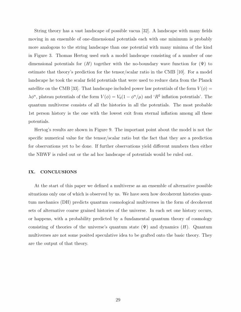
Hertog’s results are shown in Figure 9. The important point about the model is not the

specific numerical value for the tensor/scalar ratio but the fact that they are a prediction

for observations yet to be done. If further observations yield different numbers then either

the NBWF is ruled out or the ad hoc landscape of potentials would be ruled out.

IX. CONCLUSIONS

At the start of this paper we defined a multiverse as an ensemble of alternative possible

situations only one of which is observed by us. We have seen how decoherent histories quan-

tum mechanics (DH) predicts quantum cosmological multiverses in the form of decoherent

sets of alternative coarse grained histories of the universe. In each set one history occurs,

or happens, with a probability predicted by a fundamental quantum theory of cosmology

consisting of theories of the universe’s quantum state (Ψ) and dynamics (H). Quantum

multiverses are not some posited speculative idea to be grafted onto the basic theory. They

are the output of that theory.

29

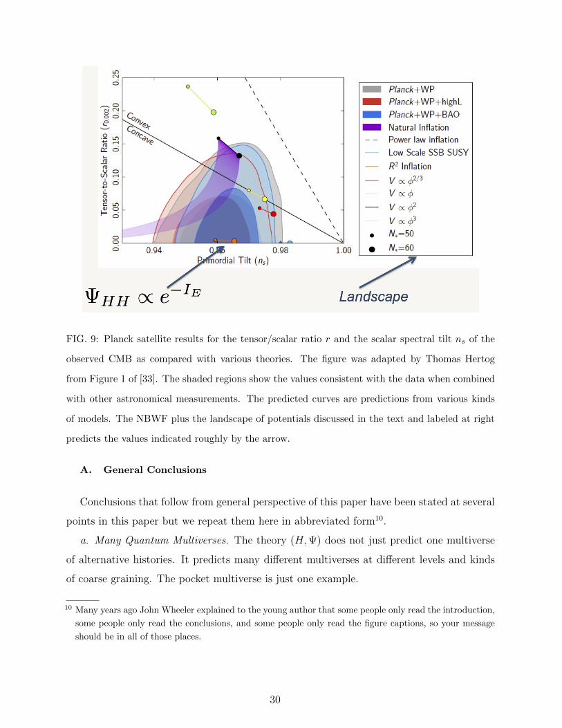
FIG. 9: Planck satellite results for the tensor/scalar ratio r and the scalar spectral tilt ns of the

observed CMB as compared with various theories. The figure was adapted by Thomas Hertog

from Figure 1 of [33]. The shaded regions show the values consistent with the data when combined

with other astronomical measurements. The predicted curves are predictions from various kinds

of models. The NBWF plus the landscape of potentials discussed in the text and labeled at right

predicts the values indicated roughly by the arrow.

A. General Conclusions

Conclusions that follow from general perspective of this paper have been stated at several

points in this paper but we repeat them here in abbreviated form10.

a. Many Quantum Multiverses. The theory (H,Ψ) does not just predict one multiverse

of alternative histories. It predicts many different multiverses at different levels and kinds

of coarse graining. The pocket multiverse is just one example.

10 Many years ago John Wheeler explained to the young author that some people only read the introduction,

some people only read the conclusions, and some people only read the figure captions, so your message

should be in all of those places.

30

b. Multiverses are Not a Choice. Quantum multiverses are not a choice or an assumption

separate from the theory (H,Ψ). They follow or do not follow from (H,Ψ). If you have

some prior objection to multiverses of some kind then restrict to theories (H,Ψ) that don’t

imply them.

c. Multiverses are Generic. Simple, manageable, discoverable (H,Ψ)’s generically predict

quantum multiverses consisting of an ensemble of many possible histories together with

probabilities for which one occurs. If the ensemble consisted of just one history with certainty

all of present complexity would have to be encoded (H,Ψ).

d. Anthropic Selection is Automatic. Anthropic selection is an automatic consequence of

first person quantum mechanical probabilities for observations (Section II C 1). Probabilities

for our observations are conditioned on a description of our observational situation and we

won’t observe what is where we cannot exist.

e. Different Mechanisms for the Variation of Constants. In different quantum multiverses

constants like Λ can be constant in each history but very from history to history, or can

vary in space within every history. Automatic anthropic selection is enabled in either case.

f. Two Routes to Coarse-Graining. Quantum multiverses are restricted to sets of alterna-

tive coarse grained histories that are decoherent — that have negligible quantum interference

between individual histories in a set. Further coarse graining can be carried out either by

summing probabilities or by summing quantum amplitudes. That is a considerable compu-

tational advantage.

Understanding quantum multiverses as decoherent sets of alternative coarse-grained his-

tories of the universe provides a unified perspective on different notions of multiverse that

have been discussed. As in the two-slit models in Section II it includes the multiverses that

describe the possible outcomes of laboratory experiment. As in Section V and VI it includes

a quantum picture of pocket universes at different levels of coarse graining. As in Sections

VII and VIII it provides a notion of a multiverse in which constants vary in a way that is

different from pocket multiverses.

B. How Specific Models Support the General Conclusions

Sections V-VIII exhibited five quantum cosmological models that illustrate the different

kinds of quantum multiverse that follow from an (H,Ψ)’s consisting the no-boundary quan-

31

tum state of the universe Ψ and dynamical theories H based general relativity coupled to

a single scalar field moving in different potentials. These models are of course consistent

with the general conclusions above as are the two-slit models in Section II. But they also

illustrate the following specific consequences:

• How pocket (bubble) multiverses universes emerge from some dynamical theories (H,Ψ)

like the one in Section V but not from others like the ones in Sections IV and VI.

•. How the same theory (H,Ψ) can predict multiverses at vastly different levels of coarse

graining like the multiverse of true vacuum bubbles in Section V and the multiverse of

possibilities for our bubble in Section VI.

•. How to use appropriate coarse grainings implemented by summing amplitudes rather

than probabilities to make manageable predictions for our observations even when the large

scale structure of the universe is a complex roiling sea of false vacuum bubbles in an ever

expanding sea of false vacuum as in Section VI.

• How deterministic classical physics emerges from (H,Ψ) as a quantum multiverse of

histories with high probability for ones exhibiting correlations in time by deterministic laws

like the Einstein equation as in Section IV.

• How a landscape potential with many minima leads to different possible values of the

cosmological constant and how first person probabilities implement anthropic restrictions

for values we will observe as in Section VII

• How a landscape of effective potentials leads to testable predictions for features of the

CMB as in Section VIII.

Quantum multiverses are what a fundamental theory (H,Ψ) predicts. It is through them

that we understand our universe. As Weinberg wrote: “Most advances in the history of

science have been marked by discoveries about nature, but at certain turning points we have

made discoveries about science itself”. The quantum multiverses of the universe are one of

these turning points.

Acknowledgments

The author thanks Murray Gell-Mann, Stephen Hawking, Thomas Hertog, and Mark

Srednicki for discussions on the quantum mechanics of the universe over many years. He

thanks Bernard Carr, George Ellis, and Thomas Hertog for useful conversations, for critical

32

readings of the manuscript, and for supplying relevant references. He thanks David Krakauer

and Steven Benner for discussions on experimental evolution. He thanks Thomas Hertog

for permission to reproduce Fig 9. He thanks the Santa Fe Institute for supporting many

productive visits there. This work was supported in part by the National Science Foundation

under grant PHY15-04541.

Appendix A: A FAQ for Discussion

There has been much discussion of cosmological multiverses by many authors. Some

works known to the author (but not necessarily read carefully by the author) are [34–46].

This FAQ addresses concerns that have been raised in some of these articles about whether a

quantum multiverse is falsifiable, testable, predictive, real, and scientific. No claim is made

to cover all of the issues that have been raised or to review all the discussion that has taken

place. This FAQ is separated from the main discussion because it reflects the opinions of

the author more than the results of calculation.

The quantum multiverse framework for prediction presented here is a synthesis of many

elements. These include a quantum mechanics for the universe (DH), a model of observers,

for example the one in IV 1, a theory of the universe’s quantum state (Ψ), and a dynamical

theory (H) expressed in particular variables, perhaps defining a landscape of vacua, etc.

Is the notion of a quantum multiverse of the universe falsifiable? Yes. As in every other

theory in physics this one can be falsified by falsifying any of the elements mentioned above

that went into its construction. Take, for example DH. There is overwhelming evidence for

quantum multiverses on laboratory scales. But there is little evidence that the same quantum

mechanics (DH) can be extrapolated to the scales of cosmology as has been assumed in this

paper. Suppose quantum laboratory experiment shows that DH is false on some intermediate

scale. Then DH would be falsified. Similarly with the other elements of the predictive

framework: a dynamical theory, a quantum state, a landscape for the variation of constants,

etc.

Are quantum multiverses of the universe testable? Yes. A theory like (H,Ψ) is testable

by the (1st person) probabilities it predicts for the outcomes of observations. These are

probabilities supplied by (H,Ψ) conditioned on a description of our observational situa-

33

tion11. Ideally we would test the theory with situations where the predicted probabilities

are near 1. If a prediction with probability near 1 does not occur the theory is falsified. But

this luxury is seldom accessible in environmental sciences like geology, planet formation, bio-

logical evolution, human history, and cosmology. Rather we judge the success of a theory by

its successful prediction of correlations among our present data as in the example in Section

VII and Section VIII. (For more on criteria for success see, e.g. [3].) Hertog’s prediction of

the tensor/scalar ratio in the CMB described Section VIII provides a clear example. If the

observed ratio is much different from the predicted one then either the landscape is wrong,

the state is wrong, or the framework of quantum prediction is wrong.

Something like a cosmological multiverses might be directly testable by experiment if a

very large spacetime volume could be prepared with an initial quantum state from which

galaxies, stars, life etc would emerge over billions of years. This is quite beyond human

powers at present. But the laws of the universe do not have to be such as to make it easy

for some negligible bits of protoplasm to test them directly on the scales that happen to be

accessible to them at the moment.

Are other histories in the multiverse of alternatives observable? No. The

different histories are exclusive alternatives. We are not outside the universe observing the

whole ensemble, but rather inside it participating in the superposition. A live Schrodinger

cat does not observe a dead cat. There are six alternative outcomes to the roll of a die each

with a probability of 1/6. We observe the one face that comes up. We do not observe the

alternative outcomes of that one roll.

Is the quantum multiverse of the universe real? Yes. It is a tenet of many Everettian

formulations of quantum theory for closed systems that all the histories in a given multiverse

are real [4, 6]. Further, all the other multiverses based on different variables with different

levels of coarse graining are real. There are also formulations of DH in which only one

history occurs in a multiverse of possible ones real [47]. For more of the author’s more

nuanced views on what’s real see [48, 49].

Are there other areas of science with similar issues? Yes. Biological evolution is

concerned with the multiverse of different histories of the origin of species. Individual

11 In various works we have called these top-down or first person probabilities. For more on this see [8].

34

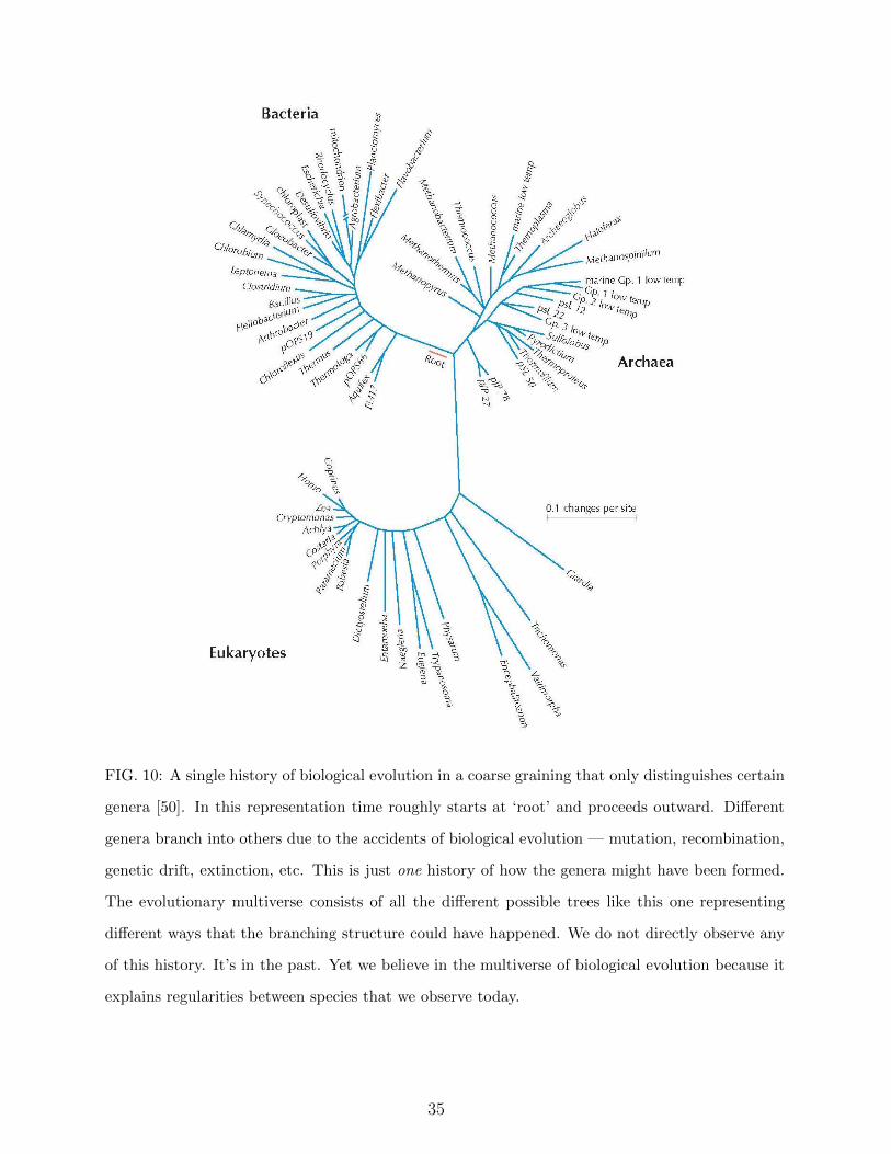
FIG. 10: A single history of biological evolution in a coarse graining that only distinguishes certain

genera [50]. In this representation time roughly starts at ‘root’ and proceeds outward. Different

genera branch into others due to the accidents of biological evolution — mutation, recombination,

genetic drift, extinction, etc. This is just one history of how the genera might have been formed.

The evolutionary multiverse consists of all the different possible trees like this one representing

different ways that the branching structure could have happened. We do not directly observe any

of this history. It’s in the past. Yet we believe in the multiverse of biological evolution because it

explains regularities between species that we observe today.

35

histories can be illustrated by familiar tree diagrams like the example in Figure 10. Differ-

ent evolutionary histories correspond to different branching trees. In principle the theory

(H,Ψ) predicts probabilities for these various trees to occur but these are much beyond our

ability to compute at present. We do not observe directly (‘see’) any of the histories of

this multiverse. They are in our past. Yet we believe that biological evolution happened

because it is explains regularities today. For example plausible reconstructions of the evo-

lutionary multiverse explain the similarities between species today. Those similarities are

consequences of frozen accidents of evolution — chance events whose consequences prolif-

erated. The theory of this multiverse is based on a number of elements: Genetic variation

by mutation, genetic drift, or recombination; a fitness landscape of ecological niches; an ini-

tial condition of primordial DNA synthesis. This is testable in a limited way by controlled

laboratory experiment [51, 52]. Other historical sciences such as geology, planet formation,

human history etc. provide similar examples of multiverses. In cosmology we do not observe

big bang nucleosynthesis directly but we believe that it happened in the past because of its

successful prediction of the correlations in the abundance of the elements observed today.

Are quantum multiverses a departure from laboratory physics? No Laboratory

experiments are inside the universe not somehow outside it. Laboratory experiments can

therefore be described by highly coarse grained alternative histories of the universe. The

highly successful Copenhagen formulation of quantum mechanics is not an alternative to DH

but an approximation to it that is appropriate for measurement situations [18]. Quantum

cosmology is not in conflict with the successes in the laboratory.

But Copenhagen quantum mechanics must be generalized beyond the the laboratory

to apply the early universe where no measurements were being made and no observers

were around to carry them out. DH, the generalization used here, is not a departure from

Copenhagen quantum mechanics where it applies but rather a generalization of it to new

domains of applicability. Some generalization is inevitable for cosmology and various ones

been studied since the time of Everett.

Cosmology is a historical science like geology, biological evolution, and human history. Its

aim is to use that data that exists now to reconstruct the quantum past in order to simplify

the prediction of the future (e.g.[21]). We should not be surprised that the extension of

observation to new domains of phenomena require new extensions of existing theory.

36

Are quantum multiverses scientific. Yes, in the author’s opinion: As sketched above,

in many areas of science one finds multiverses of the kind mentioned in the introduction —

an ensemble of possible situations only one of which is observed by us.

Appendix B: A Little More DH

In this Appendix we repeat much of the qualitative discussion of the two slit models in

Section II with more equations. That may helpful to some readers.

The inputs to the prediction of a quantum multiverse are the HamiltonianH and quantum

state |Ψ(t)〉 of the particles in the boxes. This is a function of time in the Schrodinger picture

in which we work. The state of the electron can also be described by a wave function in

configuration space, viz.

Ψ = Ψ(x, y, t) (B1)

using a coordinate x for the horizontal direction and y for the vertical direction in the three

boxes as shown in Figure 1 and assuming symmetry in the perpendicular direction. We move

back and forth between wave functions like (B1) and bras and kets like |Ψ(t)〉 as convenient.

Histories can be represented by quantum branch state vectors constructed from (H,Ψ).

For an example take the TSS model. Denote the initial state at time t0 by Ψ(x, y, t0). This

is a product of wave packet in the x-direction φ(x, t0) and a wave function ψ0(y, t0) localized

at the gun, viz.

Ψ(x, y, t0) = ψ(y, t0)φ(x, t0) (B2)

This wave function evolves in time by the Schrodinger equation

ih∂Ψ

∂t= HΨ. (B3)

We assume that φ(x, t) is a narrow wave packet peaked to the left of the slits but moving

to the right so as to reach the slits at time ts and the detecting screen at td. Thus, its progress

in x recapitulates evolution in time. After passing through the slits the wave function has

the approximate form

Ψ(x, y, t) = ψU(y, t)φ(x, t) + ψL(y, t)φ(x, t), ts < t < td. (B4a)

≡ ΨU(x, y, t) + ΨL(x, y, t). (B4b)

37

Here, in the first term ψU(y, t) is localized near the upper slit at time ts and spreads over

a larger region of y by the time td that the electron hits the detecting screen. Similarly for

the second term. The last line defines branch wave functions ΨU(x, y, t) and ΨL(x, y, t) for

the two histories in the set.

Simple two-slit model (TSS): The electron starts localized at the gun. The alternative

position intervals Y at the further screen defines a coarse grained set of alternative coarse-

grained histories of the electron between the times t0 and td. If PY are a complete set

of orthogonal projections on these intervals the branch state vectors for these histories are

|ΨY (td)〉 ≡ PY |Ψ(td)〉. The probability to arrive at Y predicted from (H,Ψ) is

p(Y ) = ||PY |Ψ(td)〉||2 = |||ΨY (td)〉||2. (B5)

A finer grained set of histories for TSS would also specify whether the electron passed

through the the upper slit U or the lower slit L on its way to a given interval Y . Naively one

might expect that the probabilities pU(Y ) and pL(Y ) that the electron the upper or lower

slit respectively and arrived at Y would be, from (B4b),

pU(Y ) = ||PY |ΨU(td)〉||2, pL(Y ) = ||PY |ΨL(td)〉||2 (B6)

Then we would have from (B4b) and (B5)

p(Y ) = ||PY |ΨU(td)〉+ PY |ΨL(td〉||2 = ||PY |ΨU(td)〉||2 + ||PY |ΨU(td)〉|||2 (B7)

This is false unless the two branches PY |ΨU(td)〉 and PY |ΨL(td〉 are orthogonal so that the

quantum interference between them vanishes. That is, it is inconsistent unless the set of

histories decoheres.

〈ΨU(td)|PY |ΨL(td)〉 ≈ 0 (B8)

That won’t be the case in TSS. The two histories interfere as shown by interference pattern

that is a characteristic feature of the two slit experiment. TSS does not have a multiverse

of this kind.

Two-slit model with gas (TSG): The TSG model contains a gas of particles that interact

weakly with the electron — an example of an environment. The initial wave function is

Ψ(x, y, t0) = ψ(y, t0)φ(x, t0)χ(t0), t0 < t < ts. (B9)

38

where χ(t0) is the initial state of all the particles in the gas. After passing through the slits

this becomes

Ψ(x, y, t) = ψU(y, t)φ(x, t)χU(t) + ψL(y, t)φ(x, t)χL(t), ts < t < td. (B10a)

≡ ΨU(x, y, t) + ΨL(x, y, t). (B10b)

where χU(t) and χL(t) denote the state of the gas particles that have scattered from the

region of the upper and lower slit respectively. Then ΨU(x, y, td) and ΨL(x, y, td) are the

branch wave functions for the two histories that the electron arrived in Y at time td after

passing through either the upper or lower slit.

In the simple two-slit model (TSS) the set of alternative histories describing which slit

(U or L) the electron went through on its way to arrive at Y on the further screen did not

decohere as required for a quantum multiverse. That was because the states representing the

two histories were not orthogonal. However, because of the gas in (TSG) the two histories do

decohere. The decoherence condition (B8) is satisfied because the state of the gas scattered

from the upper slit |χU〉 is orthogonal to the state of the gas scattered from the lower slit

|χL〉 if enough particles scatter.

To see that gas ensures this orthogonality consider a single gas particle a whose initial

state is |χa〉 that scatters near the upper slit will be in a final state SU |χa〉 where SU is the

S-matrix for scattering near the upper slit. Similarly for the lower slit with SL|χa〉 If N gas

particles scatter the overlap between |χU〉 and |χL〉 will be proportional to N inner products

of the formN∏a=1

|〈χa|S†USL|χa〉|. (B11)

Since the two final state vectors SU |χa〉 and SL|χa〉 are different each individual product has

a magnitude less than 1. The product of a very large number of such products will be near

zero implying decoherence.

Thus for TSG we have exhibited two quantum multiverses at different levels of coarse

graining. The first one (just Y ) is a coarse graining of the second (Y and S). The first

ignores the gas, the second follows it.

39

[1] J. Barrow and F. Tipler, The Anthropic Cosmological Principle, (OUP, Oxford,1985).

[2] S. Weinberg, Anthropic Bound on the Cosmological Constant, Phys. Rev. Lett., 62, 485 (1989)

[3] J.B. Hartle and T. Hertog, Anthropic Bounds on Lambda from the No-Boundary Quantum

State, Phys. Rev. D, 88, 123516 (2013), arXiv:1309.0493.

[4] S. Saunders, J. Barrett, A. Kent and D. Wallace eds, Many Worlds?, Everett, Quantum Theory

and Reality, (OUP, Oxford, 2010).

[5] D. Deutsch, The Beginning of Infinity, (Viking Penguin, New York, 2011)

[6] D. Wallace, The Emergent Multiverse: Quantum Theory according to the Everett Interpre-

tation, (OUP, Oxford, 2012).

[7] J. B. Hartle and S.W. Hawking, The Wave Function of the Universe, Phys. Rev. D 28, 2960-

2975 (1983), S.W. Hawking, The Quantum State of the Universe, Nucl. Phys. B, 239, 257-276

(1984).

[8] J.B. Hartle and T. Hertog, One bubble to rule them all, arXiv:1604.03580.

[9] J. B. Hartle, S.W. Hawking, T. Hertog, Local Observation in Eternal Inflation, Phys. Rev.

Lett. 106, 141302 (2011), arXiv:1009.252.

[10] T. Hertog, Predicting a Prior for Planck, JCAP 1402 (2014) 043, arXiv:1305.6135.

[11] R.B. Griffiths, Consistent Quantum Theory, (Cambridge University Press, Cambridge, UK ,

2002); R. Omnes, Interpretation of Quantum Mechanics, (Princeton University Press, Prince-

ton,1994); M. Gell-Mann, The Quark and the Jaguar, (W.H. Freeman New York, 1994);

M. Gell-Mann and J.B. Hartle, Quantum Mechanics in the Light of Quantum Cosmology, in

Complexity, Entropy, and the Physics of Information, ed. by W. Zurek, (Addison Wesley,

Reading, MA ,1990), P.C. Hohenberg, An introduction to consistent quantum theory, Rev.

Mod. Phys. , 82 2835-2844 (2010).

[12] J.B. Hartle, The Quantum Mechanics of Closed Systems, in Directions in General Relativity,

Volume 1, ed. by B.-L. Hu, M.P. Ryan, and C.V. Vishveshwara, (CUP, Cambridge, 1993),

arXiv:gr-qc/9210006.

[13] H. Everett III, Relative State Formulation of Quantum Mechanics, Rev. Mod. Phys, 29, 454

(1957).

[14] E. Joos and H.D. Zeh, The Emergence of Classical Properties Through Interaction with the

40

Environment, Zeit. Phys. B, 59, 223 (1985).

[15] W. Zurek, Decoherence, Einselection, and the Quantum Origins of the Classical Rev. Mod.

Phys. 75, 715 (2003)

[16] M. Gell-Mann and J.B. Hartle, Classical Equations for Quantum Systems, Phys. Rev. D, 47,

334 (1993), arXiv: gr-qc/9210010.

[17] M. Gell-Mann and J.B. Hartle, Quantum Mechanics in the Light of Quantum Cosmology,

in Complexity, Entropy, and the Physics of Information, ed. by W. Zurek, Addison Wesley,

Reading, MA, (1990).

[18] J.B. Hartle, The Quantum Mechanics of Cosmology, in Quantum Cosmology and Baby Uni-

verses: Proceedings of the 1989 Jerusalem Winter School for Theoretical Physics, ed. by

S. Coleman, J.B. Hartle, T. Piran, and S. Weinberg, World Scientific, Singapore (1991), Sec-

tion II.10.

[19] J.B. Hartle and T. Hertog, The Observer Strikes Back, in The Philosophy of Cosmology

ed. by K. Chamcham, J. Silk, J.D. Barrow, and S. Saunders, (Cambridge University Press,

Cambridge, 2017), arXiv:1503.07295.

[20] S.W. Hawking and T. Hertog, Populating the Landscape: A Top Down Approach, Phys. Rev.

D 73, 123527 (2006), arXiv:hep-th/0602091.

[21] J.B. Hartle, Quantum Pasts and the Utility of History, Physica Scripta, T76, 67–77 (1998);

arXiv:gr-qc/9712001.

[22] J.B. Hartle, Living in a Superposition, arXiv:1511.01550.

[23] J.B. Hartle, The quasiclassical realms of this quantum universe, arXiv:0806.3776. A slightly

shorter version is published in Many Worlds? edited by S. Saunders, J. Barrett, A. Kent,

and D. Wallace (Oxford University Press, Oxford, 2010), the longer version was reprinted in

Foundations of Physics, 41, 982 (2011).

[24] J.B. Hartle and M. Srednicki, Are We Typical?, Phys. Rev. D, 75, 123523 (2007),

arXiv:0704:2530.

[25] J.B. Hartle and Thomas Hertog, Classical Prediction in Quantum Cosmology, (to be finished).

[26] J.B. Hartle, S.W. Hawking, and T. Hertog, The No-Boundary Measure in the Realm of Eternal

Inflation, Phys. Rev. D, 82, 063510 (2010); arXiv:1001:0262.

[27] J.B. Hartle, S.W. Hawking, and T. Hertog, Classical Universes of the No-Boundary Quantum

State, Phys. Rev. D 77, 123537 (2008), arXiv:0803:1663.

41

[28] J.B. Hartle, S.W. Hawking, and T. Hertog, The No-Boundary Measure of the Universe, Phys.

Rev. Lett., 100, 202301 (2008), arXiv:0711:4630; Classical Universes of the No-Boundary

Quantum State, Phys. Rev. D, 77, 123537 (2008), arXiv:0803:1663, J.B. Hartle and T. Hertog,

Replication Regulates Volume Weighting in Quantum Cosmology, Phys. Rev. D, 80, 063531

(2009), arXiv:0905.3877.

[29] S. Coleman and F. De Luccia, Gravitational Effects on and of Vacuum Decay, Phys. Rev D,

21, 3305 (1980).

[30] S.W. Hawking and T. Hertog, A Smooth Exit from Eternal Inflation, arXiv:1707.7702.

[31] M. Tegmark, A. Aguirre, M.J. Rees, and F. Wilczek, Dimensionless constants, cosmology, and

other dark matters, Phys. Rev. D 73, 023505 (2006).

[32] F. Denef and M.R. Douglas, Distributions of Flux Vacua, JHEP 0405:072, 2004.

[33] P. A. R. Ade, et. al. Planck 2013 Results, XXII Constraints on Inflation, Astron. Astrophys.

A22, 571 (2014); arXiv:1303.5082

[34] B.J. Carr and M.J. Rees, The anthropic principle and the structure of the physical world.,

Nature 278 (605) 230 (1979).

[35] S. Weinberg, Living in the Multiverse published in [37], arXiv:hepth/0511037.

[36] A. Vilenkin, Many Worlds in One: The Search for Other Universes, (Hill and Wang, 2006.)

[37] The many fine articles in B.J. Carr, Universe or Multiverse?, (Cambridge University Press,

2007).

[38] Carr, B.J. and Ellis, G.F.R. 2008. Universe or multiverse?, Astronomy and Geophysics 49(2):

2.29 2.33 (2008).

[39] L. Mersini-Houghten, Thoughts on Defining the Multiverse, arXiv:0804.3419.

[40] P. Steinhardt, Theories of Anything, in What Scientific Idea is Ready for Retirement,

https://www.edge.org/response-detail/25405

[41] G. F. R. Ellis, Does the Multiverse Really Exist?, Scientific American, August 2011, p. 38ff.

[42] A. Vilenkin and M. Tegmark, The Case for Parallel Universes, Scientific American, July 19,

2011, p123.

[43] F. Wilczek, Multiversality, Class. Quant. Grav ,30, 193001 (2013); arXiv:2307.7376.

[44] G.F.R. Ellis and J. Silk, Scientific Method: Defend the Integrity of Physics ,Nature, 516,

321-323 (2014).

[45] G.F.R. Ellis, On the Philosophy of Cosmology, Studies in History and Philosophy of Modern

42

Physics., 46, 5-23 (2014).

[46] A. Linde, A Brief History of the Multiverse, arXiv:1512.01203.

[47] M. Gell-Mann and J.B, Hartle, Decoherent Histories Quantum Mechanics with One ‘Real’

Fine-Grained History, Phys. Rev. A 85, 062120 (2012); arXiv:1106.0767.

[48] J.B. Hartle, Quantum Physics and Human Language, J. Phys. A: Math. Theor., 40, 3101-3121

(2007), arXiv:quant-ph/0610131.

[49] The author’s papers on quantum mechanics and quantum cosmology are collected together

with some commentary at http://web.physics.ucsb.edu/˜quniverse. (Still under construction.)

[50] Norman Pace, from http://pacelab.colorado.edu

[51] S.F. Elena and R.E. Lenski, Evolution Experiments with Microorganisms: The Dynamics and

Genetic Bases of Adaption, Nature Reviews (Genetics), 4, 487 (2004).

[52] L.M. Wahl and D.C. Krakauer, Models of Experimental Evolution: The Role of Genetic Chance

and Selective Necessity, Genetics, 156, 1437, (2000).

[53] J..B. Hartle and T. Hertog, Replication Regulates Volume Weighting in Quantum Cosmology,

Phys. Rev. D 80, 063531 (2009), arXiv:0905.3877.

43