Embed Size (px)
Citation preview
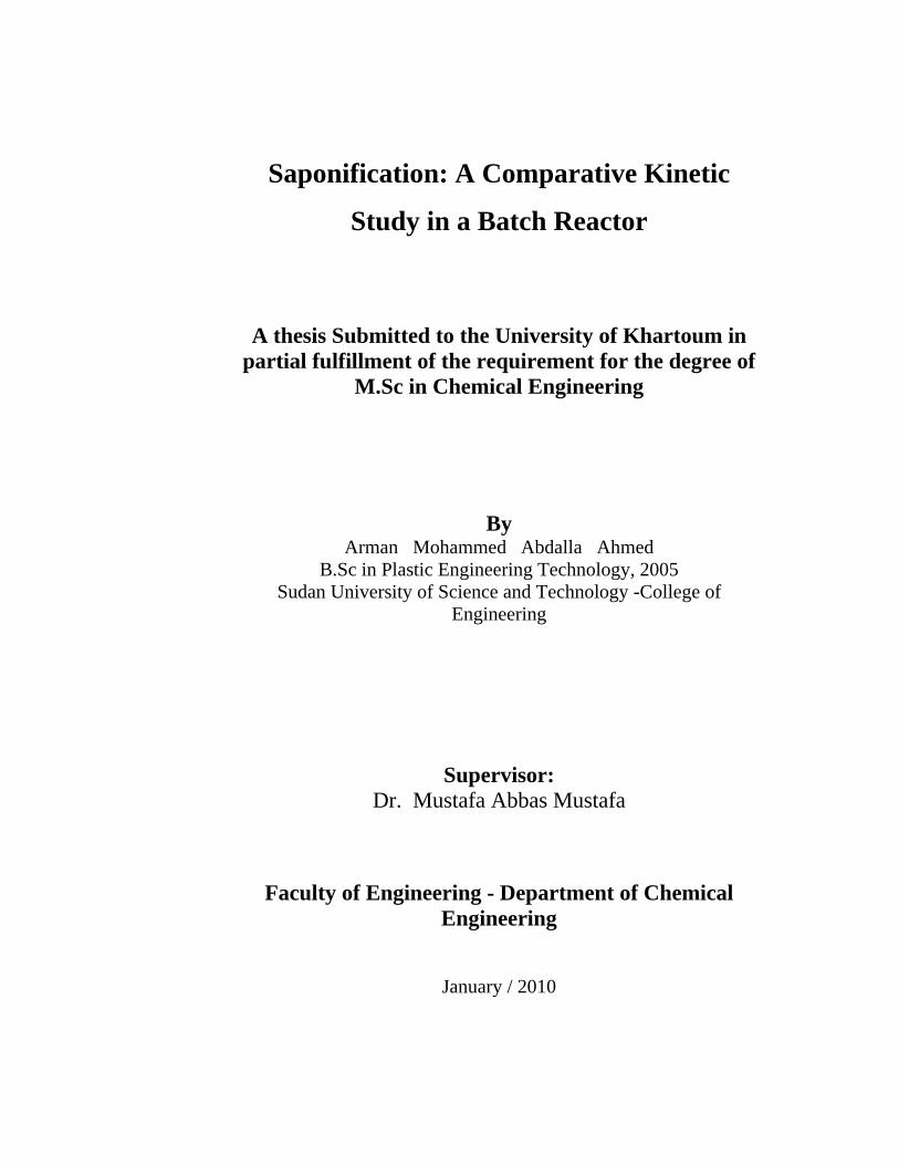
Saponification: A Comparative Kinetic
Study in a Batch Reactor
A thesis Submitted to the University of Khartoum in partial fulfillment of the requirement for the degree of
M.Sc in Chemical Engineering
By Arman Mohammed Abdalla Ahmed
B.Sc in Plastic Engineering Technology, 2005 Sudan University of Science and Technology -College of
Engineering
Supervisor: Dr. Mustafa Abbas Mustafa
Faculty of Engineering - Department of Chemical
Engineering
January / 2010

i
:قال تعالى
ا ال ال يكلف الله نفسا إالوسعها لها ما آسبت وعليها( ما اآتسبت ربن
تؤاخذنا إن نسينا أو أخطأنا ربنا وآل تحمل علينا إصرا آما حملته على
ا الذين من قبلنا ر ر لن ا واغف ف عن ه واع بنا وال تحملنا ما ال طاقة لنا ب
)وارحمنا أنت موالنا فانصرنا على القوم الكافرين
)286(سورة البقرة اآلية

ii
Dedication
To the soul of my father
To my well – beloved mother
To my wife, brothers, sisters and extended family
To every body who contributed on this thesis directly or indirectly
,,,,,,,,,,,,,,,,,,,,
TÜÅtÇ

iii
Acknowledgement I would like to thank the University of Khartoum and to express my
sincere gratitude to my supervisor Dr. Mustafa Abbas Mustafa. I would
like to acknowledge his unlimited efforts in guiding and following up the
thesis progress, and specially his spirit – raising encouragement.
As many people have contributed constructively to this work. I would
like to thank them all and in particular the people of University of
Khartoum - Department of Chemical Engineering - Unit Operations lab,
who provided me with the necessary information to rehabilitate the batch
reactor. I owe special thanks to every body who contributed to this
thesis directly or indirectly.
TÜÅtÇ
iv
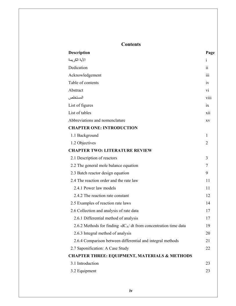
Contents Description Page
i اآلية الكريمة
Dedication ii
Acknowledgement iii
Table of contents iv
Abstract vi
viii المستخلص
List of figures ix
List of tables xii
Abbreviations and nomenclature xv
CHAPTER ONE: INTRODUCTION
1.1 Background 1
1.2 Objectives 2
CHAPTER TWO: LITERATURE REVIEW
2.1 Description of reactors 3
2.2 The general mole balance equation 7
2.3 Batch reactor design equation 9
2.4 The reaction order and the rate law 11
2.4.1 Power law models 11
2.4.2 The reaction rate constant 12
2.5 Examples of reaction rate laws 14
2.6 Collection and analysis of rate data 17
2.6.1 Differential method of analysis 17
2.6.2 Methods for finding -dCA/ dt from concentration time data 19
2.6.3 Integral method of analysis 20
2.6.4 Comparison between differential and integral methods 21
2.7 Saponification: A Case Study 22
CHAPTER THREE: EQUIPMENT, MATERIALS & METHODS
3.1 Introduction 23
3.2 Equipment 23
v
3.3 Materials 26
3.4 Methods 27
3.4.1 The Algorithm for kinetic evaluation of Saponification reaction 27
3.4.2 General consideration for Saponification Experiments 28
3.4.3 Analysis Procedure for Saponification Experiments 28
3.4.4 Titration Method 28
3.4.5 Experiment A: Determination of concentration dependency factor
for caustic soda 31
3.4.6 Experiment B: Determination of concentration dependency factor
for Ethyl Acetate 37
3.4.7 Experiment C: Determination of dependency factor
for temperatures 43
CHAPTER FOUR : RESULTS & DISCUSSION
4.1 Results 53
4.1.1 Experiment A 53
4.1.2 Experiment B 57
4.1.3 Experiment C 61
4.2 Discussion 65
4.2.1 Discussion Experiment A 65
4.2.2 Discussion Experiment B 78
4.2.3 Discussion Experiment C 79
4.2.4 Discussion Activation Energy 80
CHAPTER FIVE: CONCLUSION & RECOMMENDATIONS
5.1 Conclusion 84
5.2 Recommendations 84
REFERENCES
References 85
APPENDIXES
Appendix A : Materials Safety Data Sheet (MSDS) 86
Appendix B : CHEMCAD Software (Saponification Reaction Simulation) 89
Appendix C : Rate constant versus Temperatures in Saponification
Literature Values 95
vi
Abstract
Knowledge of kinetic parameters is of extreme importance for the
chemical engineer prior to design of chemical reactors. This research
focuses on the study of the kinetics of the saponification reaction
between sodium hydroxide and ethyl acetate in a batch reactor.
To achieve this, the batch reactor available at the unit operation
laboratory (Department of Chemical Engineering, University of
Khartoum) had been repaired and modified to suit the experimental
procedures. The maintenance of the reactor includes change of bearing
and bushes. The modification was made on the motion transmission from
the electric motor to the agitator and on the temperature control system
where a digital thermometer was used.
Prior to the kinetic study, two methods were tried for the temperature
control. The first method used an electric heater plus a cooling jacket
around the reactor but failed to precisely control the temperature. The
second method used consists of a water bath of controlled temperature
where the reactants are heated to the required temperature before they
were fed to the reactor which was also heated to the same temperature
using the water jacket. This method was successful in achieving a tight
control of the temperature, thus ensuring isothermal conditions.
The reactions kinetics was studied through initially studying caustic
soda concentrations dependency using an excess of ethyl acetate while
maintaining isothermal conditions .Then the concentration dependency
of ethyl acetate was evaluated using equal concentrations of reactants
before operating at various condition to evaluate the temperature
dependency.
Analytical mathematical and computer methods were used to analyze
the experimental observations and data. The results obtained (of
evaluated kinetic parameters) showed, a clear agreement with the values

vii
from literature. Improved numerical accuracy has been shown in some
cases to result as the use of polynomial fit relative to finite difference
method.
It is recommended that future work focuses on fully automating the
batch reactor using appropriate hardware and software (Labview)
components.

viii
مستخلص البحث
ائى دس الكيمي سبة للمهن ه بالن رات الكينماتيكي ة المتغي م معرف ة التفاعل (من المه ل ) حرآي قب
ا على يرآز هذا البحث .الشروع فى تصميم المفاعل الكيميائى صبن م ة تفاعل الت دراسة حرآي
).الحله( الوجبه مفاعل فىيدروآسيد الصوديوم واستات اإليثيلهبين
ات الموحد ،إلنجاز هذا ه ( المفاعل الموجود فى معمل العملي سم الهندسه الكيميائي ة ،ق جامع
ستخدمه ) الخرطوم ة طرق التجارب الم لمفاعل اشتملت لصيانة ال .تم إصالحه وتعديله لمالئم
ه من المحرك الكه والتعديالت . على تغيير البلى والجلب ل الحرآ ى خالط الخاصه بنق ائى ال رب
.المفاعل وآذلك تغيير نظام التحكم فى درجة حرارة المفاعل حيث استخدم مقياس حراره رقمى
ه التفاعل ى درجة حراره المفاعل ،قبل دراسة حرآي تحكم ف ان لل رت طريقت ه .اختب الطريق
م ت ا ل د حول المفاعل ولكنه ى قميص تبري ائى باالضافه ال ى االولى استخدم سخان آهرب نجح ف
ه استخدم الطريقه الثانيه .ضبط درجة المفاعل بالدقه المطلوبه ه درجة حراره ثابت ائى ل ام م حم
ا ة حرارته ى درج تحكم ف اء الم ه ونفس الم واد المتفاعل سخين الم ه ت تم في ستخدم داخل تحيث ي
. وهى طريقه ناجحه للحصول على درجة حراره ثابته .القميص حول المفاعل
ه وإستخدام تم دراسة صودا الكاوي ز ال ى ترآي اد عل ائى بدراسة اإلعتم حرآية التفاعل الكيمي
دراسة اإلعتماد على ترآيز استات م ث.ثيل وذلك عند ثبوت درجة الحراره فائض من أستات اإلي
ى درجة الحراره اإليثيل بإستخدام تراآيز متساويه من المادتين ومن ثم درس اعتماد التفاعل عل
. الحراره بتغير درجة
ه ارات المعملي ائج اإلختب ل نت ل وطرق الحاسوب لتحلي ه الرياضيه للتحلي تخدمت الطريق .اس
ا ائج المتحصل عليه لل(النت ة التفاع رات حرآي يم متغي ع ) ق ى المراج وده ف يم الموج ع الق ق م تتف
.دود دية للحصول على تطابق مع دوال القوى متعددة الح آذلك استخدمت الطرق العد. العلميه
ق ك عن طري ى المفاعل وذل اتيكيى ف تحكم األتوم تخدام ال ستقبال بإس ة توصى م ذة الدراس ه
. برامج الحاسوب وملحقاته
ix
List of figures NO Description Page
Figure (2.1): Simple batch homogeneous reactor 3
Figure (2.2): Continuous-stirred tank reactor (CSTR) 5
Figure (2.3): Plug-flow tubular reactor (PFR) 6
Figure (2.4): Packed-bed reactor (PBR) 7
Figure (2.5): Balance in system volume 7
Figure (2.6): Calculation of the activation energy 13
Figure (2.7): Zero Order Reaction 14
Figure (2.8): First Order Reaction 15
Figure (2.9): Second Order Reaction equal molar 16
Figure (2.10): Second Order Reaction non equal molar 16
Figure (2.11): Differential method to determine reaction order 18
Figure (2.12): Integral method (the necessary graph for
order guessed) 21
Figure (3.1): Batch reactor with water around it from
thermostat bath 25
Figure (3.2): Withdraw the sample by medical injection , acid with an
indicator in E-flask and the titration unit 30
Figure (3.3): Experiment C Concept Excel program to Plot graph
for 1/CAvs t and Trend (Line) to get k'' 43
Figure (4.1): Experiment A(isothermal at 37.70C) batch (I)
Concentration time data from Experimental in Table (3.6)
and literature values from Appendix B . 53
Figure (4.2): Experiment A(isothermal at 37.70C) batch (I)
Experimental rate of reaction (NaOH) versus its
concentration in Table (3.6) . 54
Figure (4.3): Experiment A(isothermal at 37.70C) batch (II)
Concentration time data from Experimental in
Table (3.6) and literature values from Appendix B. 54
Figure (4.4): Experiment A(isothermal at 37.70C) batch (II)
x
Experimental rate of reaction (NaOH) versus
its concentration in Table (3.6) . 55
Figure (4.5): Experiment A(isothermal at 37.70C) batch (III)
Concentration time data from Experimental in
Table (3.6) and literature values from Appendix B. 56
Figure (4.6): Experiment A(isothermal at 37.70C) batch (III)
Experimental rate of reaction (NaOH) versus its
concentration in Table (3.6) . 56
Figure (4.7): Experiment B (isothermal at 37.70C) batch (I)
Concentration time data from Experimental in
Table (3.12) and literature values from Appendix B. 57
Figure (4.8): Experiment B (isothermal at 37.70C) batch (I)
Experimental rate of reaction (NaOH) versus its
concentration in Table (3.12) . 58
Figure (4.9): Experiment B (isothermal at 37.70C) batch (II)
Concentration time data from Experimental in
Table (3.12) and literature values from Appendix B. 58
Figure (4.10):Experiment B (isothermal at 37.70C) batch (II)
Experimental rate of reaction (NaOH) versus its
concentration in Table (3.12). 59
Figure (4.11):Experiment B (isothermal at 37.70C) batch (III)
Concentration time data from Experimental in Table (3.12)
and literature values from Appendix B. 60
Figure (4.12):Experiment B (isothermal at 37.70C) batch (III)
Experimental rate of reaction (NaOH) versus its
concentration in Table (3.12). 60
Figure (4.13):Experiment C (at 31.20C) batch (I)
Concentration time data from Experimental and
literature values from Table (3.16). 61
Figure (4.14):Experiment C(at 31.20C) batch (I) Excel program
to plot 1/CA vs t from Table (3.16). 62
Figure (4.15):Experiment C (at 37.70C) batch (II)
xi
Concentration time data from Experimental and
Actual fromTable (3.20). 62
Figure (4.16):Experiment C (at 37.70C) batch (II) Excel program
to plot 1/CA vs t from Table (3.20). 63
Figure (4.17): Experiment C (at 45.50C) batch (III)
Concentration time data from Experimental and
Actual Table (3.24). 64
Figure (4.18): Experiment C (at 45.50C) batch (III) Excel program
to plot 1/CA vs t from Table (3.26). 64
Figure (4.19): Experiment A batch (I) data input to poly math program 66
Figure (4.20): Experiment A batch (I) Excel program to plot rate of
reaction (NaOH) versus its concentration
in Table (4.2). 69
Figure (4.21): Experiment A batch (II) data input to poly math program 70
Figure (4.22): Experiment A batch (II) Excel program to plot
rate of reaction (NaOH) versus its concentration
in Table (4.3). 73
Figure (4.23): Experiment A batch (III) data input to poly mat program 74
Figure (4.24): Experiment A batch (III) Excel program to plot
rate of reaction (NaOH) versus its concentration
in Table (4.5). 77
Figure (4.25): Excel plot Activation Energy form Table (4.11) . 81
Figure (4.26): Excel plot Activation Energy for Experiment C batch(I)
and batch(II) from table (4.11). 82
Figure (B.1): CHEMCAD Experiment A concentration time data 89
Figure (B.2): CHEMCAD Experiment A Excel plot log log data
in Table (B.1) 91
Figure (B.3): CHEMCAD Experiment B concentration time data 91
Figure (B.4): CHEMCAD Experiment B Excel plot log log data
in Table (B.2) 94
xii
List of tables NO Description Page
Table (2.1): Advantages and disadvantages of batch reactor 4
Table (2.3): Advantages and disadvantages of CSTR 5
Table (2.3): Advantages and disadvantages of PFR 6
Table (2.4): Comparison between differential and integral methods 22
Table (3.1): Experiment A Concept Concentration of un reacted NaOH 32
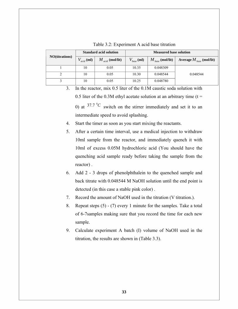
Table (3.2): Experiment A acid base titration 33
Table (3.3):Experiment A batch (I) volume of NaOH use in the titration 34
Table (3.4): Experiment A batch (I) Concentration of unreacted NaOH 35
Table (3.5): Experiment A batch (I) rate of reaction of NaOH 36
Table (3.6): Experiment A the three batches ( t,vtit,Con,rate) of NaOH 36
Table (3.7): Experiment B Concept Concentration of unreacted NaOH 38
Table (3.8): Experiment B acid base titration 39
Table (3.9): Experiment B batch (I) volume of NaOH used
in the titration 40
Table (3.10): Experiment B batch (I) Concentration of unreacted NaOH 41
Table (3.11): Experiment B batch (I) rate of reaction of NaOH 42
Table (3.12): Experiment B the three batches ( t,vtit,Con,rate) of NaOH 42
Table (3.13): Experiment C batch (I) acid base titration 44
Table (3.14): Experiment C batch (I) volume of NaOH used
in the titration 45
Table (3.15): Experiment C batch (I) Concentration of unreacted NaOH 46
Table (3.16): Experiment C batch (I) Concentration of NaOH and its
inverse (Experimental, Actual) 46
Table (3.17): Experiment C batch (II) acid base titration 47
Table (3.18): Experiment C batch (II) volume of NaOH used
in the titration 48
Table (3.19): Experiment C batch (II) Concentration of
unreacted NaOH 49
Table (3.20): Experiment C batch (II) Concentration of NaOH and its
xiii
inverse (Experimental, Actual) 49
Table (3.21): Experiment C batch (III) acid base titration 50
Table (3.22): Experiment C batch (III) volume of NaOH used
in the titration 51
Table (3.22): Experiment C batch (III) Concentration of
unreacted NaOH 52
Table (3.24): Experiment C batch (III) Concentration of NaOH and its
inverse (Experimental, Actual) 52
Table (4.1): Experiment A Average Order with respect to (NaOH) 65
Table (4.2): Poly math batch (I) first negative derivative points 69
Table (4.3): Poly math batch (II) first negative derivative points 73
Table (4.4): Poly math batch (III) first negative derivative points 77
Table (4.5): Summary of discussion of experiment A 78
Table (4.6): Experiment B Average overall reaction order with
respect to (NaOH) 78
Table (4.7): Summary of discussion of experiment B 78
Table (4.8): Experiment C rate constant for second order reaction
with respect to (NaOH) 79
Table (4.9): Measuring the temperatures of every sample was
withdraw from reactor 79
Table (4.10): Experiment C reason (1) rate constant for second order
reaction with respect to (NaOH) 80
Table (4.11): Activation Energy Experiment C and Actual or literature
value from Appendix C 81
Table (4.12): Summary discussion of saponification experiments 82
Table (4.13): The comprehension rate equation 83
Table (A.1): Chemical Safety Data for Sodium Hydroxide 86
Table (A.2): Chemical Safety Data for Ethyl acetate 87
Table (B.1): CHEMCAD Experiment A concentration time
data combine with finite difference and Excel 90
Table (B.2): CHEMCAD Experiment B concentration time data

xiv
combine with finite difference and Excel 92
Table (C.1): Rate constant vs Temperatures in Saponification
Literature Values 95
xv
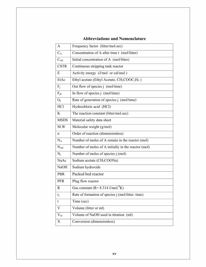
Abbreviations and Nomenclature A Frequency factor (litter/mol.sec)
CA Concentration of A after time t (mol/litter)
CA0 Initial concentration of A (mol/litter)
CSTR Continuous stripping tank reactor
E Activity energy (J/mol or cal/mol )
EtAc Ethyl acetate (Ethyl Acetate, CH3COOC2H5 )
Fj Out flow of species j (mol/time)
Fj0 In flow of species j (mol/time)
Gj Rate of generation of species j (mol/time)
HCl Hydrochloric acid (HCl)
K The reaction constant (litter/mol.sec)
MSDS Material safety data sheet
M.W Molecular weight (g/mol)
n Order of reaction (dimensionless)
NA Number of moles of A remain in the reactor (mol)
NA0 Number of moles of A initially in the reactor (mol)
Nj Number of moles of species j (mol)
NaAc Sodium acetate (CH3COONa)
NaOH Sodium hydroxide
PBR Packed bed reactor
PFR Plug flow reactor
R Gas constant (R= 8.314 J/mol.0K)
rj Rate of formation of species j (mol/litter. time)
t Time (sec)
V Volume (litter or ml)
Vtit Volume of NaOH used in titration (ml)
X Conversion (dimensionless)
1
CHAPTER ONE
INTRODUCTION 1.1. Background
A batch reactor may be described as a vessel in which any chemicals
are placed to react. Batch reactors are normally used in studying the
kinetics of chemical reactions, where the variation of a property of the
reaction mixture is observed as the reaction progresses. Data collected
usually consist of changes in variables such as concentration of a
component, total volume of the system or a physical property like
electrical conductivity. The data collected are then analyzed using
pertinent equations to find desired kinetic parameters.
There is currently a pilot- scale batch reactor at the University of
Khartoum - Department of Chemical Engineering - unit operations lab.
One of the main objectives of this is thesis to rehabilitate and repair this
reactor.
In order to validate this reactor a Saponification Reaction was
chosen, because it is homogeneous (liquid phase reaction) in this case as
constant volume reactor and Safety its reactants and products (Appendix
A: Material Safety Data Sheet (MSDS)).
A saponification is a reaction between an ester and an alkali, such as
sodium hydroxide, producing a free alcohol and an acid salt.
The stoichiometry of the saponification reaction between sodium
hydroxide and Ethyl Acetate is:
CH3COOC2H5 + NaOH CH3COONa + C2H5OH ------------- Eq(1.1)
Saponification is primarily used for the production of soaps.
2
1.2. Objectives
The Repair of batch reactor in University of Khartoum -
Department of Chemical Engineering - Unit Operations Lab.
The validation of the repaired reactor by using a
Saponification reaction and get experimental kinetic data, the
values obtained was compared to values from Literature.
3
CHAPTER TWO
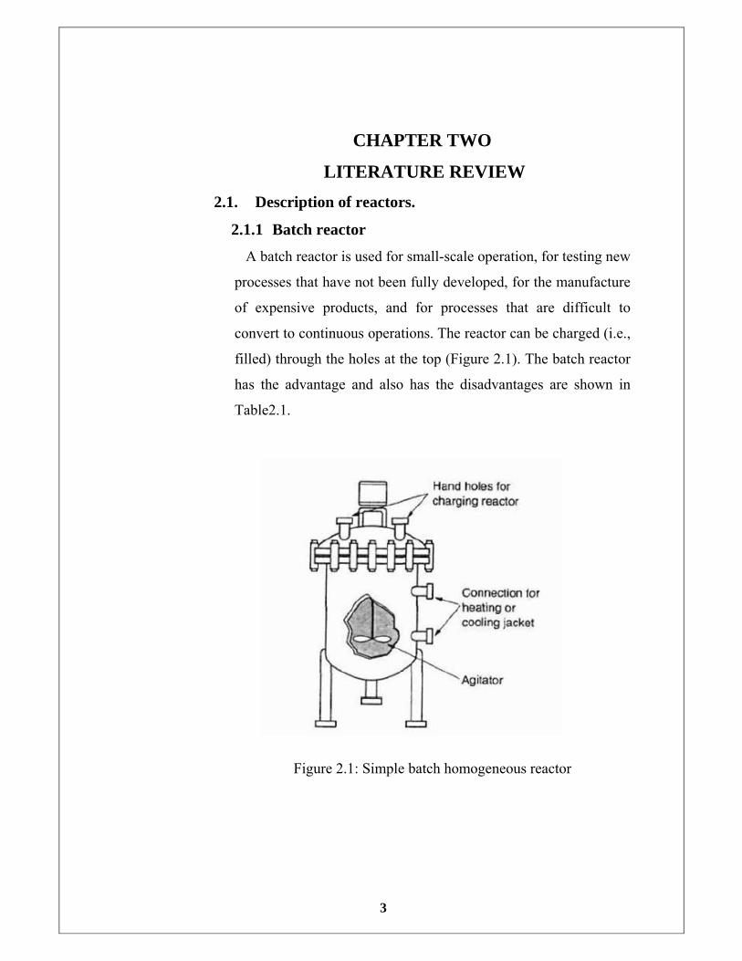
LITERATURE REVIEW 2.1. Description of reactors.
2.1.1 Batch reactor
A batch reactor is used for small-scale operation, for testing new
processes that have not been fully developed, for the manufacture
of expensive products, and for processes that are difficult to
convert to continuous operations. The reactor can be charged (i.e.,
filled) through the holes at the top (Figure 2.1). The batch reactor
has the advantage and also has the disadvantages are shown in
Table2.1.
Figure 2.1: Simple batch homogeneous reactor
4
Table 2.1: Advantages and disadvantages of batch reactor
Advantages disadvantages
High conversions can be obtained. High cost of labor per unit of production.
Versatile, used to make many
products.
Difficult to maintain large scale
production.
Good for producing small
amounts.
Long idle time (Charging & Discharging
times) leads to periods of no production.
Easy to Clean No instrumentation – Poor product
quality
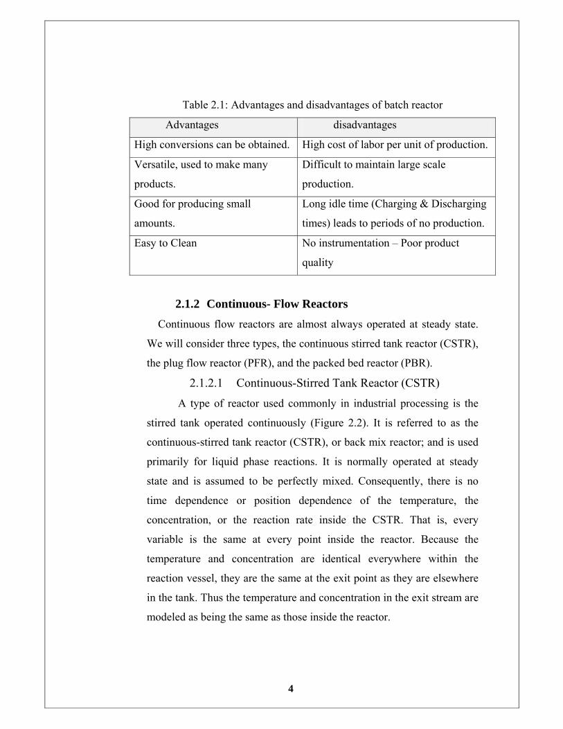
2.1.2 Continuous- Flow Reactors
Continuous flow reactors are almost always operated at steady state.
We will consider three types, the continuous stirred tank reactor (CSTR),
the plug flow reactor (PFR), and the packed bed reactor (PBR).
2.1.2.1 Continuous-Stirred Tank Reactor (CSTR)
A type of reactor used commonly in industrial processing is the
stirred tank operated continuously (Figure 2.2). It is referred to as the
continuous-stirred tank reactor (CSTR), or back mix reactor; and is used
primarily for liquid phase reactions. It is normally operated at steady
state and is assumed to be perfectly mixed. Consequently, there is no
time dependence or position dependence of the temperature, the
concentration, or the reaction rate inside the CSTR. That is, every
variable is the same at every point inside the reactor. Because the
temperature and concentration are identical everywhere within the
reaction vessel, they are the same at the exit point as they are elsewhere
in the tank. Thus the temperature and concentration in the exit stream are
modeled as being the same as those inside the reactor.
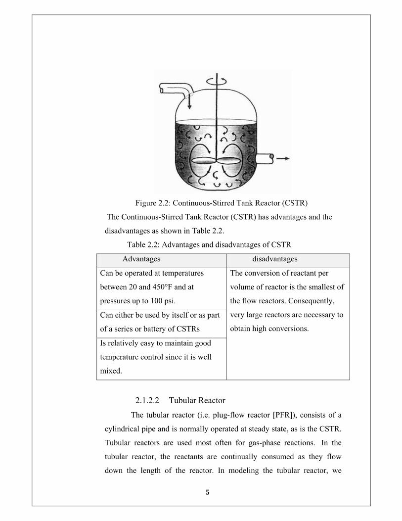
5
Figure 2.2: Continuous-Stirred Tank Reactor (CSTR)
The Continuous-Stirred Tank Reactor (CSTR) has advantages and the
disadvantages as shown in Table 2.2.
Table 2.2: Advantages and disadvantages of CSTR
Advantages disadvantages
Can be operated at temperatures
between 20 and 450°F and at
pressures up to 100 psi.
Can either be used by itself or as part
of a series or battery of CSTRs
Is relatively easy to maintain good
temperature control since it is well
mixed.
The conversion of reactant per
volume of reactor is the smallest of
the flow reactors. Consequently,
very large reactors are necessary to
obtain high conversions.
2.1.2.2 Tubular Reactor
The tubular reactor (i.e. plug-flow reactor [PFR]), consists of a
cylindrical pipe and is normally operated at steady state, as is the CSTR.
Tubular reactors are used most often for gas-phase reactions. In the
tubular reactor, the reactants are continually consumed as they flow
down the length of the reactor. In modeling the tubular reactor, we
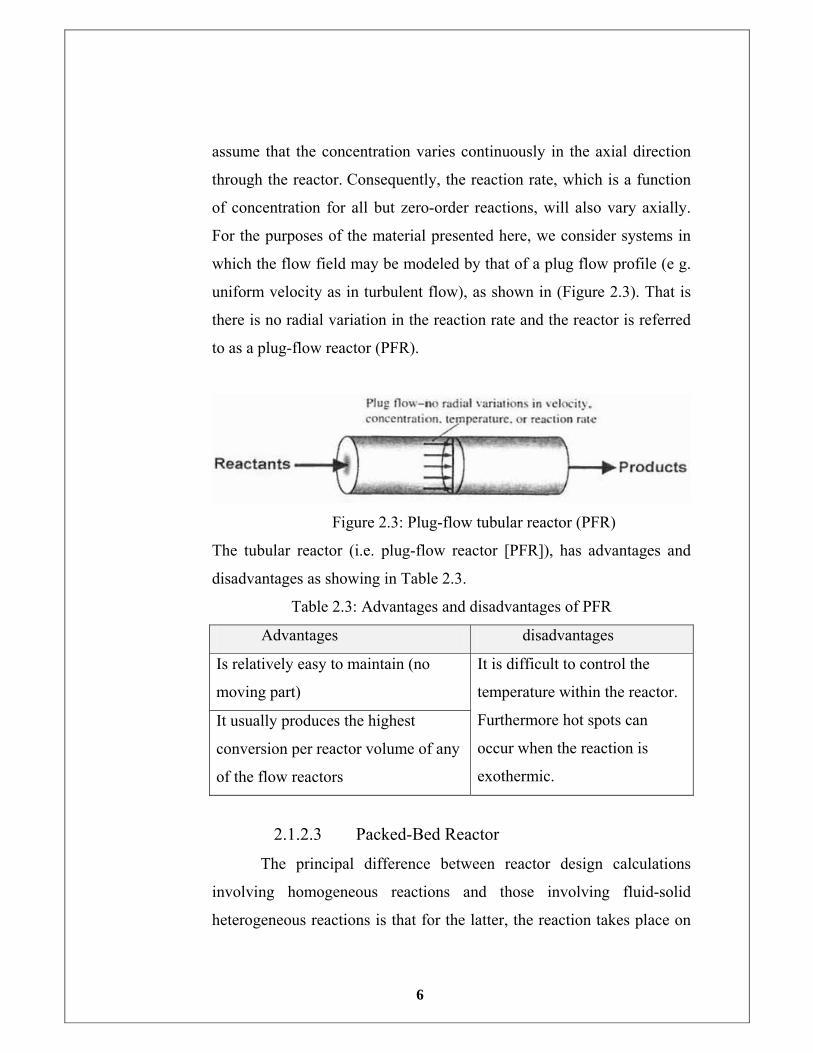
6
assume that the concentration varies continuously in the axial direction
through the reactor. Consequently, the reaction rate, which is a function
of concentration for all but zero-order reactions, will also vary axially.
For the purposes of the material presented here, we consider systems in
which the flow field may be modeled by that of a plug flow profile (e g.
uniform velocity as in turbulent flow), as shown in (Figure 2.3). That is
there is no radial variation in the reaction rate and the reactor is referred
to as a plug-flow reactor (PFR).
Figure 2.3: Plug-flow tubular reactor (PFR)
The tubular reactor (i.e. plug-flow reactor [PFR]), has advantages and
disadvantages as showing in Table 2.3.
Table 2.3: Advantages and disadvantages of PFR
Advantages disadvantages
Is relatively easy to maintain (no
moving part)
It usually produces the highest
conversion per reactor volume of any
of the flow reactors
It is difficult to control the
temperature within the reactor.
Furthermore hot spots can
occur when the reaction is
exothermic.
2.1.2.3 Packed-Bed Reactor
The principal difference between reactor design calculations
involving homogeneous reactions and those involving fluid-solid
heterogeneous reactions is that for the latter, the reaction takes place on
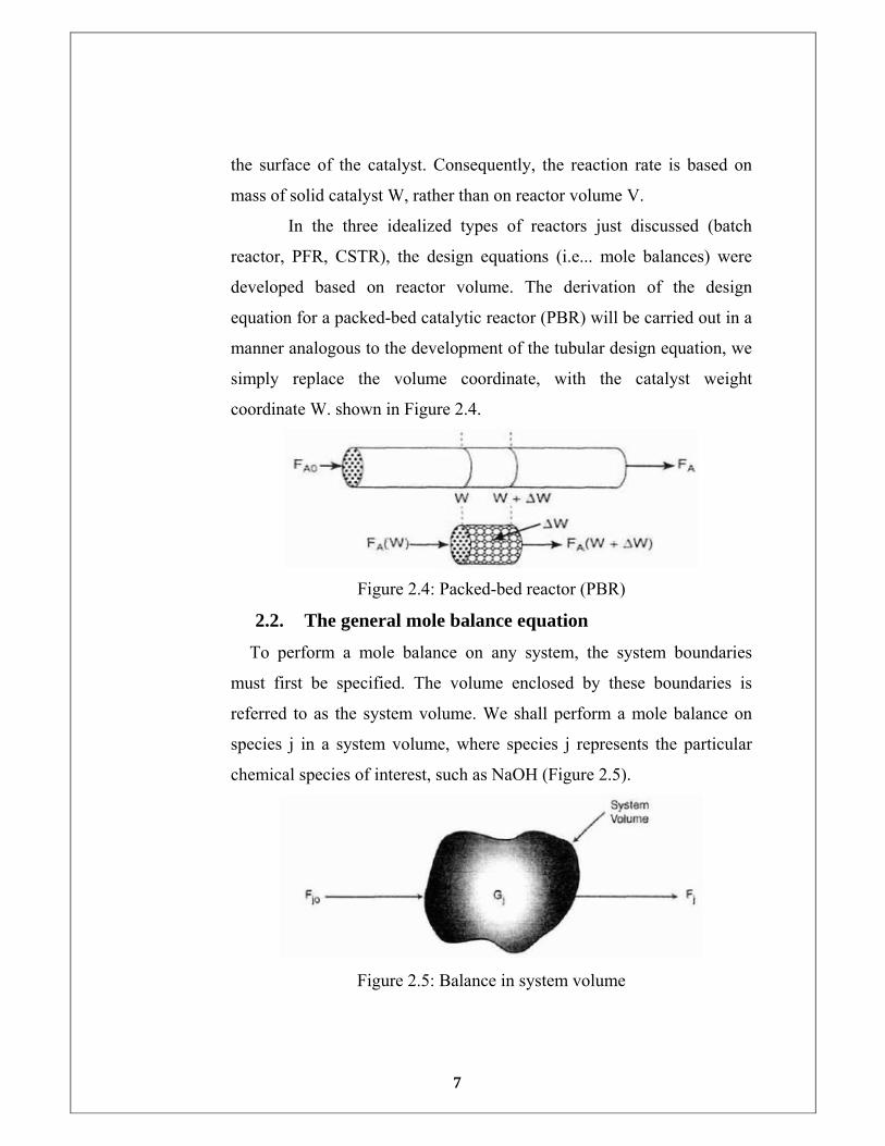
7
the surface of the catalyst. Consequently, the reaction rate is based on
mass of solid catalyst W, rather than on reactor volume V.
In the three idealized types of reactors just discussed (batch
reactor, PFR, CSTR), the design equations (i.e... mole balances) were
developed based on reactor volume. The derivation of the design
equation for a packed-bed catalytic reactor (PBR) will be carried out in a
manner analogous to the development of the tubular design equation, we
simply replace the volume coordinate, with the catalyst weight
coordinate W. shown in Figure 2.4.
Figure 2.4: Packed-bed reactor (PBR)
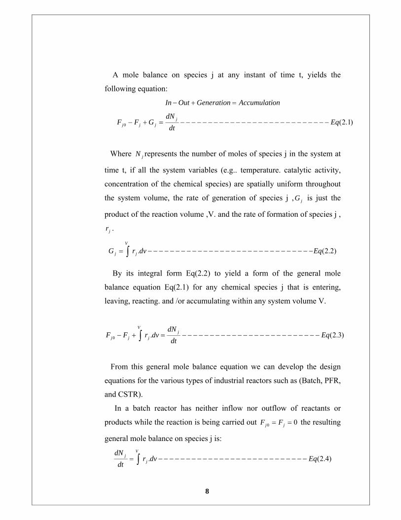
2.2. The general mole balance equation
To perform a mole balance on any system, the system boundaries
must first be specified. The volume enclosed by these boundaries is
referred to as the system volume. We shall perform a mole balance on
species j in a system volume, where species j represents the particular
chemical species of interest, such as NaOH (Figure 2.5).
Figure 2.5: Balance in system volume
8
A mole balance on species j at any instant of time t, yields the
following equation:
onAccumulatiGenerationOutIn =+−
)1.2(0 Eqdt
dNGFF j
jjj −−−−−−−−−−−−−−−−−−−−−−−−−−−=+−
Where jN represents the number of moles of species j in the system at
time t, if all the system variables (e.g.. temperature. catalytic activity,
concentration of the chemical species) are spatially uniform throughout
the system volume, the rate of generation of species j , jG is just the
product of the reaction volume ,V. and the rate of formation of species j ,
jr .
)2.2(. EqdvrG j
V
j −−−−−−−−−−−−−−−−−−−−−−−−−−−−−−= ∫
By its integral form Eq(2.2) to yield a form of the general mole
balance equation Eq(2.1) for any chemical species j that is entering,
leaving, reacting. and /or accumulating within any system volume V.
)3.2(.0 Eqdt
dNdvrFF j
j
V
jj −−−−−−−−−−−−−−−−−−−−−−−−−=+− ∫
From this general mole balance equation we can develop the design
equations for the various types of industrial reactors such as (Batch, PFR,
and CSTR).
In a batch reactor has neither inflow nor outflow of reactants or
products while the reaction is being carried out 00 == jj FF the resulting
general mole balance on species j is:
)4.2(. Eqdvrdt
dNj
Vj −−−−−−−−−−−−−−−−−−−−−−−−−−−= ∫
9
If the reaction mixture is perfectly mixed so that there is no variation in
the rate of reaction throughout the reactor volume. We can take jr out of
the integral, integrate and write the mole balance in the form.
)5.2(. EqVrdt
dNj
j −−−−−−−−−−−−−−−−−−−−−−−−−−−−=
2.3. Batch reactor design equation
In most batch reactors, the longer a reactant stays in the reactor, the
more the reactant is converted to product until either equilibrium is
reached or the reactant is exhausted. Consequently, in batch systems the
conversion X is a function of the time the reactants spend in the reactor.
If 0AN is the number of moles of A initially in the reactor. then the total
number of moles of A that have reacted after a time t is ][ 0 XN A ⋅
]fedA of Moles
reactedA of Molesfed].[A of [Moles](consumed) reactedA of [Moles =
)6.2(]].[[](consumed) reactedA of [mole 0 EqXN A −−−−−−−=
Now, the number of moles of A that remain in the reactor after a time
t, AN can be expressed in terms of 0AN and X:
XNNN AAA ⋅−= 00
The number of moles of A in the reactor after a conversion X has been
achieved is :
)7.2()1(000 EqXNXNNN AAAA −−−−−−−−−−−−−=⋅−=
When no spatial variations in reaction rate exist, the mole balance on
species A for a batch system is given by Eq(2.5):
)8.2(. EqVrdt
dNA
A −−−−−−−−−−−−−−−−−−−−−−−−−−=
This equation is valid whether or not the reactor volume is constant . In
the general reaction. Reactant A is disappearing: therefore, we multiply
both sides of Equation (2.8) by -1 to obtain the mole balance for the
hatch reactor in the form:
10
)9.2(. EqVrdt
dNA
A −−−−−−−−−−−−−−−−−−−−−−−−−−−=−
For batch reactors, we are interested in determining how long to leave
the
reactants in the reactor to achieve a certain conversion X. To determine
this length of time, we write the mole balance Eq(2.8) in terms of
conversion by differentiating Equation (2.7) with respect to time,
remembering that 0AN is the number of moles of A initially present and is
therefore a constant with respect to time.
dtdXN
dtdN
AA
00 −=
Combining the above with Equation (2.8) yields
VrdtdXN AA .0 =−
For a batch reactor, the design equation in differential form is :
)10.2(.0 EqVrdtdXN AA −−−−−−−−−−−−−−−−−−−−−−−−−=
We call Equation (2.10) the differential form of the design equation for
batch reactor because we have written the mole balance in terms of
conversion ,the differential forms of the batch reactor mole balances Eq
(2.5) and Eq(2.10) are often used in the interpretation of reaction rate
data and for reactors with heat effects, respectively. Batch reactors are
frequently used in industry for both gas-phase and liquid-phase reactions.
Liquid-phase reactions are frequently carried out in batch reactors when
small-scale production is desired or operating difficulties, rule out the
use of continuous flow systems.
For a constant-volume batch reactor 0VV = Equation (2.8) can be
arranged into the form Eq(2.11) :
11
(2.11))/(1 0
0
Eqrdt
dCdt
VNddt
dNV A
AAA −−−−−−−−−−−−−−−−−−−−−===
As previously mentioned. the differential form of the mole balance,
Equation (2.11). is used for analyzing rate data in a batch reactor .
2.4. The reaction order and the rate law
The Reaction Order and the Rate Law In the chemical reactions
considered in the following paragraphs, we take as the basis of
calculation a species A, which is one of the reactants that is disappearing
as a result of the reaction. The limiting reactant is usually chosen as our
basis for calculation. The rate of disappearance of A Ar− depends on
temperature and composition. For many reactions it can be written as the
product of a reaction, reaction rate constant Ak and a function of the
concentrations of the various species involved in the reaction:
)12.2(,...)],()][([ EqCCfnTkr BAAA −−−−−−−−−−−−−=−
The algebraic equation that relates Ar− to the species concentrations is
called the kinetic expression or rate law. The specific rate of reaction
(also called the rate constant Ak , like the reaction rate Ar− always refers
to a particular species in the reaction and normally should be subscripted
with respect to that species.
2.4.1 Power law models
The dependence of the reaction rate . Ar− on the concentrations of the
species present. fn( jC ) is almost without exception determined by
experimental observation. Although the functional dependence on
concentration may be postulated from theory, experiments are necessary
to confirm the proposed form. One of the most common general forms of
this dependence is the power law model. Here the rate law 1s the product
of concentrations of the individual reacting species. each of which is
raised to a power. For example:
12
)13.2(EqCCkr bB
aAAA −−−−−−−−−−−−−−−−−−−−−=−
The exponents of the concentrations in Equation (2.13) lead to the
concept of reaction order. The order of a reaction refers to the powers to
which the concentrations are raised in the kinetic rate law. In Equation
(2.13), the reaction is a order with respect to reactant A. and b order
with respect to reactant B. The overall order of the reaction, α
)14.2(Eqba −−−−−−−−−−−−−−−−+=α
The units of Ar− are always in terms of concentration per unit time
while
the units of the specific reaction rate, Ak will vary with the order of the
reaction.
2.4.2 The reaction rate constant
The reaction rate constant k is not truly a constant: it is merely
independent of the concentrations of the species involved in the reaction.
The quantity k is referred to as either the specific reaction rate or the rate
constant. It is almost always strongly dependent on temperature. It
depends on whether or not a catalyst is present, and in gas-phase
reactions, it may be a function of total pressure. ln liquid systems it can
also be a function of other parameters, such as ionic strength and choice
of solvent. These other variables normally exhibit much Less effect on
the specific reaction rate than temperature does with the exception of
supercritical solvents, such as super critical water.
Consequently, for the purposes of the material presented here,it will be
assumed that Ak , depends only on temperature. This assumption is valid
in more laboratory and industrial reactions and seems to work quite well.
It was the great Swedish chemist Arrhenius who first suggested that the
temperature dependence of the specific reaction rate, Ak , could be
correlated by an equation of the type
13
)15.2(][ EqAeTk RTE
A −−−−−−−−−−−−−−−−−−−−−−=−
Where
A = frequency factor
E = activation energy. J/mol or cal/mol
R = gas constant = 8.3 14 J/mol .oK = 1.987 cal/mol .oK
T= absolute temperature, oK
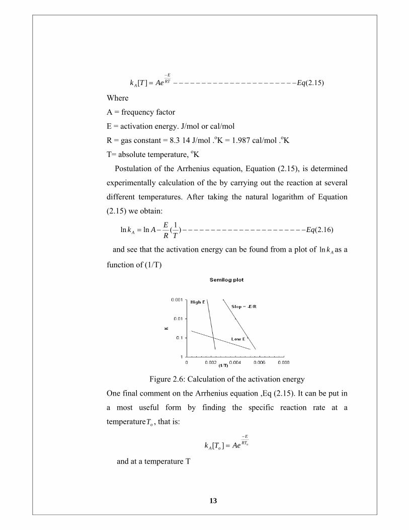
Postulation of the Arrhenius equation, Equation (2.15), is determined
experimentally calculation of the by carrying out the reaction at several
different temperatures. After taking the natural logarithm of Equation
(2.15) we obtain:
)16.2()1(lnln EqTR
EAk A −−−−−−−−−−−−−−−−−−−−−−−=
and see that the activation energy can be found from a plot of Akln as a
function of (1/T)
Figure 2.6: Calculation of the activation energy
One final comment on the Arrhenius equation ,Eq (2.15). It can be put in
a most useful form by finding the specific reaction rate at a
temperature oT , that is:
oRTE
oA AeTk−
=][
and at a temperature T
14
RTE
A AeTk−
=][
and taking the ratio to obtain
)17.2(][][)
11(
EqeTkTk TTRE
oAAo −−−−−−−−−−−−−−−−−−−=−
This equation says that if we know the specific reaction rate )( 0Tko at a
temperature 0T , and we know the activation energy, E. we can find the
specific reaction rate )(Tk at any other temperature, T. for that reaction.
2.5. Examples of reaction rate laws
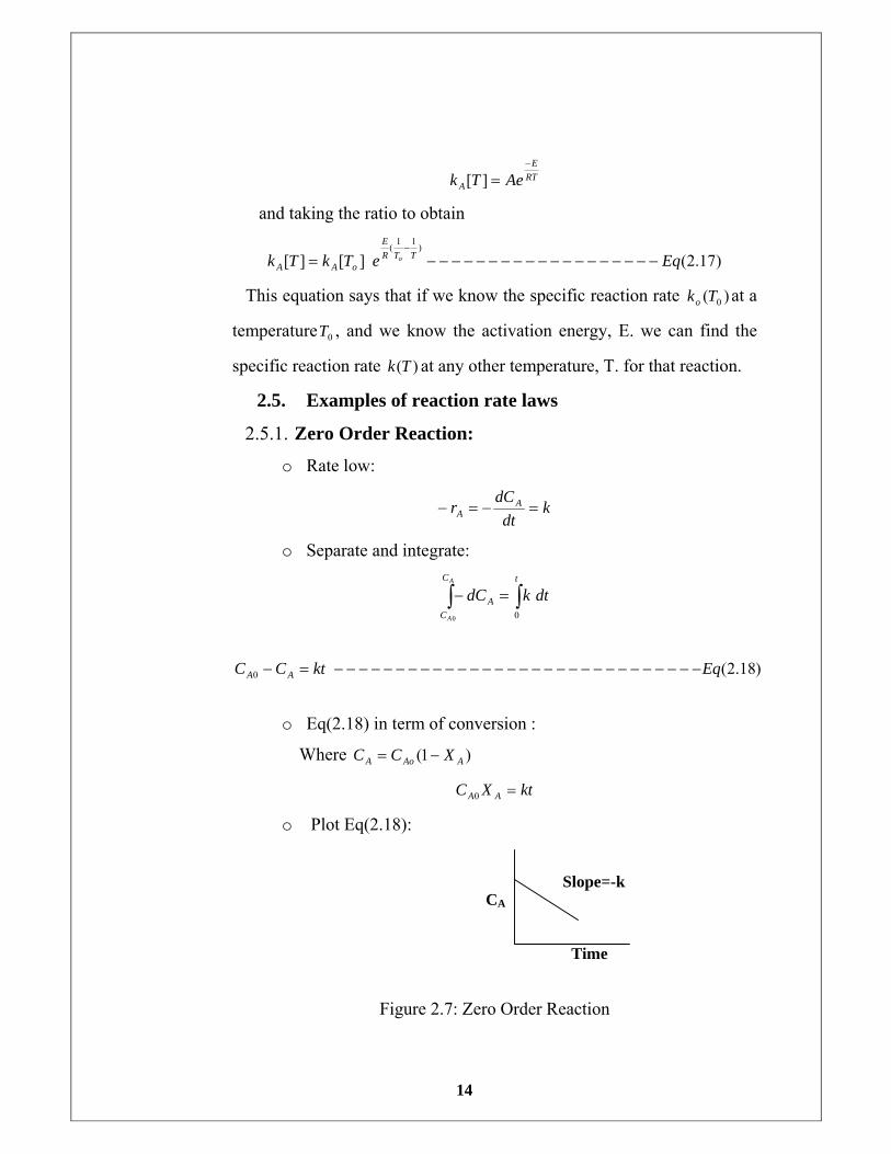
2.5.1. Zero Order Reaction:
o Rate low:
kdt
dCr A
A =−=−
o Separate and integrate:
∫∫ =−tC
CA dtkdC
A
A 00
)18.2(0 EqktCC AA −−−−−−−−−−−−−−−−−−−−−−−−−−−−−−=−
o Eq(2.18) in term of conversion :
Where )1( AAoA XCC −=
ktXC AA =0
o Plot Eq(2.18):
Figure 2.7: Zero Order Reaction
Time
Slope=-k CA
15
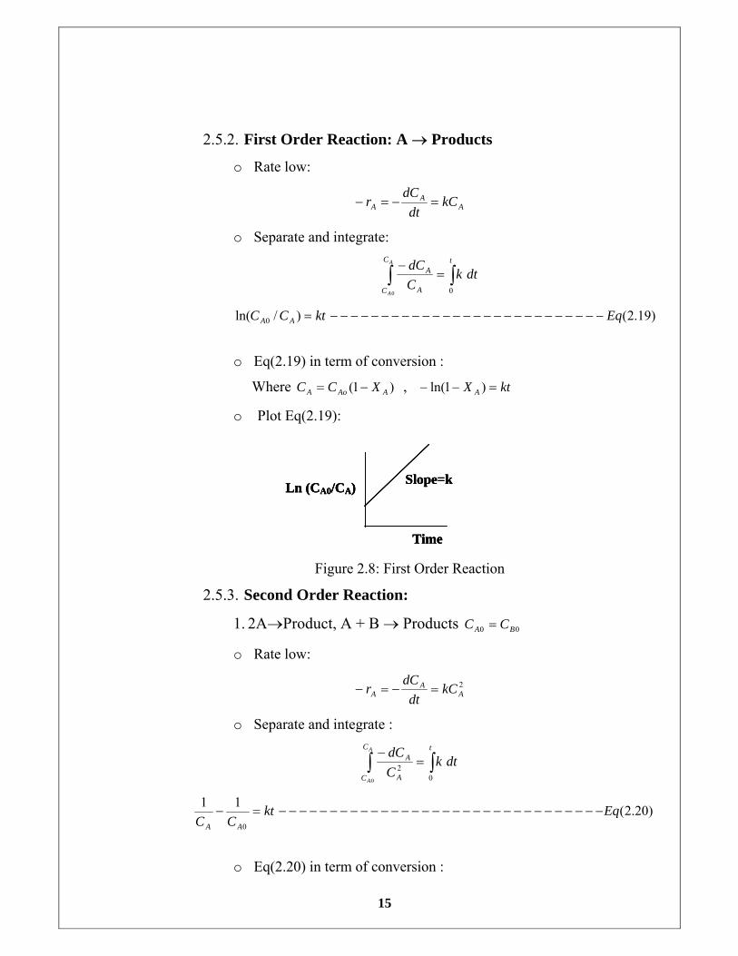
2.5.2. First Order Reaction: A → Products
o Rate low:
AA
A kCdt
dCr =−=−
o Separate and integrate:
∫∫ =− tC
C A
A dtkCdCA
A 00
)19.2()/ln( 0 EqktCC AA −−−−−−−−−−−−−−−−−−−−−−−−−−−=
o Eq(2.19) in term of conversion :
Where )1( AAoA XCC −= , ktX A =−− )1ln(
o Plot Eq(2.19):
Figure 2.8: First Order Reaction
2.5.3. Second Order Reaction:
1. 2A→Product, A + B → Products 00 BA CC =
o Rate low:
2A
AA kC
dtdC
r =−=−
o Separate and integrate :
∫∫ =− tC
C A
A dtkCdCA
A 02
0
)20.2(11
0
EqktCC AA
−−−−−−−−−−−−−−−−−−−−−−−−−−−−−−−−=−
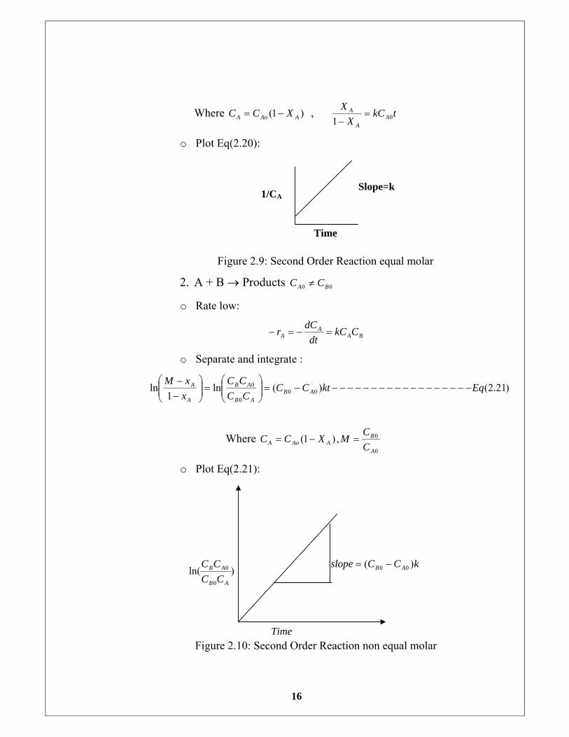
o Eq(2.20) in term of conversion :
Slope=k
Time
Ln (CA0/CA)
Slope=k
Time
Ln (CA0/CA) Slope=k
Time
Ln (CA0/CA)
16
Where )1( AAoA XCC −= , tkCX
XA
A
A01
=−
o Plot Eq(2.20):
Figure 2.9: Second Order Reaction equal molar
2. A + B → Products 00 BA CC ≠
o Rate low:
BAA
A CkCdt
dCr =−=−
o Separate and integrate :
)21.2()(ln1
ln 000
0 EqktCCCC
CCxxM
ABAB
AB
A
A −−−−−−−−−−−−−−−−−−−=⎟⎟⎠
⎞⎜⎜⎝
⎛=⎟⎟
⎠
⎞⎜⎜⎝
⎛−−
Where 0
0,)1(A
BAAoA C
CMXCC =−=
o Plot Eq(2.21):
Figure 2.10: Second Order Reaction non equal molar
Slope=k
Time
1/CA
kCCslope AB )( 00 −=
Time
)ln(0
0
AB
AB
CCCC
17
2.6. Collection and analysis of rate data
Assume that the rate law is of the form
)22.2(EqCkr AAA −−−−−−−−−=− α
Batch reactors are used primarily to determine rate law parameters for
homogeneous reactions. This determination is usually achieved by
measuring concentration as a function of time and then using either the
differential, integral method of data analysis to determine the reaction
order, α , and specific reaction rate constant, Ak .
However, by utilizing the method of excess, it is also possible to
determine the relationship between Ar− and the concentration of other
reactant That is for the irreversible reaction below Equation :
A + B → Products
With the rate law Eq(2.13)
)13.2(EqCCkr bB
aAAA −−−−−−−−−−−−−−−−−−−−−=−
where a and b are both unknown, the reaction could first be run in an
excess of B so that BC remains essentially unchanged during the course
of the reaction and :
)23.3(EqCkCCkCCkr aA
aA
bBA
bB
aAAA −−−−−−−−−−−−−−−−−−′===−
Where
)24.3(0 EqCkCkk bBA
bBA −−−−−−−−−−−−−−−−−−−−−−−−−−≈=′
After determining a , the reaction is carried out in an excess of A, or
equal molar to get overall reaction order . αA
baA
bB
aAA CkCkCkCr ′′=′′==− + )(
Where , α overall reaction order.
2.6.1. Differential method of analysis
To outline the procedure used in the differential method of analysis.
we consider a reaction carried out isothermally in a constant-volume
18
batch reactor and the concentration recorded as a function of time. By
combining (the mole balance with the rate low given by (Eq 2.22).
)22.2(EqCkdt
dCAA
A −−−−−−−−−=− α
After taking the natural logarithm of both sides of Equation (2.22)
( ) ( ) )25.2(lnlnln EqCkdt
dCAA
A −−−−−−−−−+=⎟⎠⎞
⎜⎝⎛− α
Observe that the slope of a plot of ⎟⎠⎞
⎜⎝⎛−
dtdCAln as a function of
( )ACln is the reaction order, α (Figure 2.8 ).
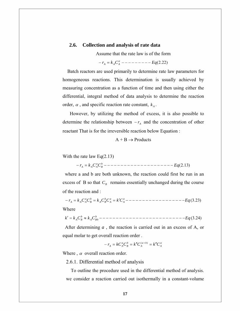
Figure 2.11: Differential method to determine reaction order
Figure 2.11 (a) shows a plot of [- (dCA/dt)] versus [CA] on log-log
paper (or use Excel to make the plot) where the slope is equal to the
reaction order α .The specific reaction rate Ak can be found by first
choosing a concentration in the plot , say CAP, and then finding the
corresponding value of [- (dCA/dt)] as shown in Figure 2.8 (b). After
raising CAP to the α power, we divide it in to [- (dCA/dt)] to
determine Ak :
( ) )26.2()(
EqC
dtdC
kAp
pA
A −−−−−−−−−−
= α
19
2.6.2. Methods for finding dtdCA /− from concentration time data
To obtain the derivative -dCA/dt used in this plot in fig(2.8), we must
differentiate the concentration-time data either numerically or
graphically. We describe two methods to determine the derivative from
data giving the concentration as a function of time. These methods are:
2.6.2.1 Numerical method
Numerical differentiation formulas can be used when the data points in
the independent variable are equally spaced . Such as 01 tt − = 12 tt − = t∆ :
Time(sec) to t1 t2 t3
Concentration
(mol/lit)
CA0 CA1 CA2 CA3
The three-point differentiation formulas
Initial point:
)27.2(243 210
0
Eqt
CCCdt
dC AAA
t
A −−−−−−−−−−−∆
−+−=⎥⎦
⎤⎢⎣⎡
=
Interior points:
)28.2(2
)( )1()1( EqtCC
dtdC iAiA
it
A −−−−−−−−−−−−−−∆
−=⎥⎦
⎤⎢⎣⎡ −+
=
Last point:
)29.2(243 )()1()2( Eq
tCCC
dtdC nAnAnA
nt
A −−−−−−−−∆
−+−=⎥⎦
⎤⎢⎣⎡ −−
=
Can be used to calculate dCA/dt . Equations (2.27) and (2.29) are used
for the first and last data points, respectively, while Equation (2.28) is
used for all intermediate data points.
20
2.6.2.2 Polynomial fit
Another technique to differentiate the data is to fit the concentration
time data to an nth-order polynomial:
)31.2(........3.2
)30.2(.........
2321
33
2210
Eqtataadt
dCEqtatataaC
A
A
−−−−−−−−−−−−+++=
−−−−−−−−−−−++++=
Many personal computer software packages contain programs that
will calculate the best values for the constants ia . One has only to enter
the concentration time data and choose the order of the polynomial. After
determining the constants ia , one has only to differentiate Eq(2.30) to
get Eq(2.31) .
2.6.3 Integral method of analysis
To determine the reaction order by the integral method, we guess the
reaction order and integrate the differential equation used to model the
batch system. If the order we assume is correct, the appropriate plot
(determined from this integration) of the concentration-time data should
be linear. The integral method is used most often when the reaction order
is known and it is desired to evaluate specific reaction rate constants at
different temperatures to determine order and the activation energy.
In the integral method of analysis of rate data, we are looking for the
appropriate function of concentration corresponding to a particular rate
law that is linear with time. You should be thoroughly familiar with the
methods of obtaining these linear plots for reactions of zero. first, and
second order. For the reaction:
21
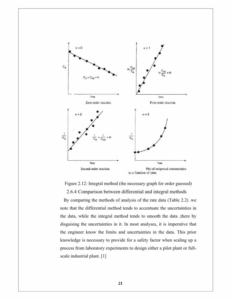
Figure 2.12: Integral method (the necessary graph for order guessed)
2.6.4 Comparison between differential and integral methods
By comparing the methods of analysis of the rate data (Table 2.2) .we
note that the differential method tends to accentuate the uncertainties in
the data, while the integral method tends to smooth the data ,there by
disguising the uncertainties in it. In most analyses, it is imperative that
the engineer know the limits and uncertainties in the data. This prior
knowledge is necessary to provide for a safety factor when scaling up a
process from laboratory experiments to design either a pilot plant or full-
scale industrial plant. [1]
22
Table 2.4: Comparison between differential and integral methods. [2]
Integral Method Differential Method
• Easy to use and is recommended for
testing specific mechanism
• Require small amount of data
• Involves trial and error
• Cannot be used for fractional orders
• Very accurate
• Useful in complicated cases
• Require large and more accurate
data
• No trial and error
• Can be used for fractional orders
• Less accurate
2.7. Saponification: A Case Study.
Rate of reaction was found to be first order with respect to each
reactants rate of reaction second order overall with rate 0.112
L/mole-sec at 25°C and the activation energy was 11.56 kcal/mol
(48390.16 J/mol). Rate constant versus Temperatures in literature
Appendix C.[3]
23
CHAPTER THREE
EQUIPMENT, MATERIALS & METHODS 3.1. Introduction
To run saponification reaction we need to equipment, materials like
chemical, methods to collect and analyze data.
3.2. Equipment
1. Repaired batch reactor at unit operations lab
The batch reactor was repaired to the model shown in (Figure 3.1).
Firstly, it was contained on parts (electrical heater, Motor, reactor vessel,
Impeller). Impeller was repaired by taking apart it and lubricate it,
thereafter, the maintenance of the reactor includes change of bearing and
pushes the modification was made on the motion transmission from the
electric motor to the agitator and on the temperature control system
where digital thermometer was used , medical injection was withdraw
the samples from reactor.
Two methods were tried for the temperature control, the first
method used an electric heater plus a cooling jacket around the reactor
but it failed to precisely control the temperature according to procedure
below:
One of reactants was placed in reactor vessel , the electrical heater
was opened to heat reactant temperature till reached to above required
temperature about + 0.50C the electrical heater was closed the valve of
cold water was opened to decrease its temperature till reached below
required temperature about -0.50C the valve was closed and opened the
electrical heater again . We Observed in this method the temperature of
reactant was not constant because the reactor put on heater and the heater
it gave heat after we closed it (the temperature of resource was not
constant).The second method used consists of water bath of controlled
24
temperature where the reactants are heated to the required temperature
before they were fed to the reactor which was also heated to the same
temperature using the water jacket , this method was successful to
control the temperature according to procedure below:
One of reactants was placed in reactor vessel ,the switch of thermostat
water bath was set at constant temperature let us say (300C) the valve of
hot water was opened to heat the reactant its temperature was increased
slowly after 20 min the temperature of reactant was reached to above
required temperature (300C) of thermostat bath about 1.20C at last the
temperature of reactant was constant at the (31.2 0C), we observed in this
method the temperature of reactor if the switch was set at an another
values in the thermostat bath (350C, 450C) the constant temperature of
reactor according to this the values (37.70C, 45.50C) respectively in this
case get good results at constant temperatures for reactor(31.20C,
37.70C and 45.50C).
Figure 3.1: water bath of controlled temperature for the batch reactor
2. Other equipments used include
1. Stopwatch.
2. Volumetric flasks.
3. Graduated cylinders.
4. Pipits.
5. 50 mL Buret.
6. 250 mL E-flasks.
7. scale
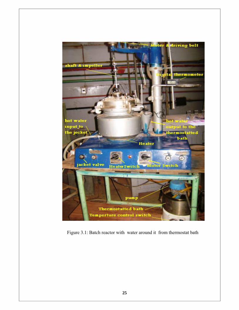
25
Figure 3.1: Batch reactor with water around it from thermostat bath
26
3.3. Materials
3.3.1. Chemicals
1. Phenolphthalein
Use as indicator is added to the acid in the E-flask . Causes the
solutions to change color when the acid is neutralized.
2. Hydrochloric Acid (HCl)
Properties: Liquid, Concentration 32 %, M.W 36.46,Wt.per ml at C020
equal 1.189 g/ml
3. Sodium Hydroxide (NaOH)
Properties: Solid Pellets, M.W 40.00
4. Ethyl Acetate(CH3COOC2H5)
Properties: liquid, Concentration 99 %, M.W 88.11, Wt.per ml at 20 0C
equal 0.902 g/ml
5. Distillated Water
Distillated water was Prepared in unit operation lab.
3.3.2. Prepare solution of the reactants
The reactants were prepared through the following procedure:
1. If the solution of reactants was prepared from solid material like
Sodium Hydroxide .
For example when preparing solution of 0.1 M NaOH /litter
)1.3(4040.1M.WMoralitybottle thefromtaken weightThe Eqg −−−−−−=×=×=
4 g is discharged to 1000 ml volumetric flask and complete the flask
by distillate water to its volume.
2. If the solution of reactants was prepared from liquid material like
Hydrochloric Acid , Ethyl Acetate.
For example when preparing solution of 0.1 M HCl/litter
27
Eq(3.2)ml/10.4410036.46
10001.18932100weightMolecular
1000gravity specific%ionconcentratbottle theofmoralityThe
−−−−−−−−−=×××
=
×××
=
mol
ml9.58bottlefromvolume10000.1bottlefromvolumemol/ml10.44 =→×=×
Withdraw 9.58 ml and discharged in to 1000 ml volumetric flask and
complete it by distillate water to its volume. 3.4. Methods
The batch reactor had been modified to the model shown in Fig(3.1),As
result, it was operated at constant temperatures (31.2 0C , 37.7 0C and
45.5 0C). It was used to get kinetic data for the liquid phase
saponification reaction of caustic soda with ethyl acetate.
3.4.1 The Algorithm for kinetic evaluation of Saponification
Reaction.
1. Stoichiomettic equation
NaOH + CH3COOC2H5 → CH3COONa + C2H5OH
aA + bB → rR + sS
2. Postulate rate law
Power law models for Homogeneous reaction )3.3(EqCkCr bB
aAA −−−=−
3. Select reactor type and corresponding mole balance
Batch reactor )4.3(Eqrdt
dCA
A −−−−−−−−−−−−−−−−−−=−
4. Process your data in terms of measured variables
In this case timetovsCA
5. Look for simplification
Consider )3.3(EqCCkr bB
aAAA −−−=−
Where a and b and Ak are unknown factors.
6. Run the saponification experiments as follows:
1. Isothermal operation
28
Run the experiment at constant temperature to fix Ak as described in
groups of Experiments (A & B ) and thus determine the coefficient a
and b respectively .
2. Non isothermal operation
Run the experiment at different temperatures (Experiment C) to see the
affect of temperature on reaction constant Ak thus calculate activation
energy of reaction , frequency factor Eq(2.15) .
3.4.2 General consideration for saponification Experiments
The experiments should include the following investigations. 1. For all batch experiments use equal volumes of each reactant to give
a 1000mL (1 litter) total reaction mixture volume at the start of the
experiment (time = 0.0). 2. The reactants should be as close to the same temperature as possible
before starting the experiment. This can be done by placing one
reactant in the reaction vessel (Batch reactor) and the other reactant in
the constant temperature bath and letting them reach the same
temperature before mixing them together .[4]
3.4.3 Analysis procedure for saponification experiments
In order to monitor the rate of the reaction in these experiments, it is
necessary to determine the amount of un-reacted NaOH at appropriate
time intervals. The reaction mixture can be monitored by using a titration
method.[5]
3.4.4 Titration Method
A small sample is collected from the reaction vessel and quenched
(reaction terminated) in a known volume and concentration of HCl. The
excess HCl is titrated with NaOH. From this titration the amount of un-
reacted NaOH can be determined and used in the determination of
kinetic data. 10 mL burette is use to titrate the samples.
29
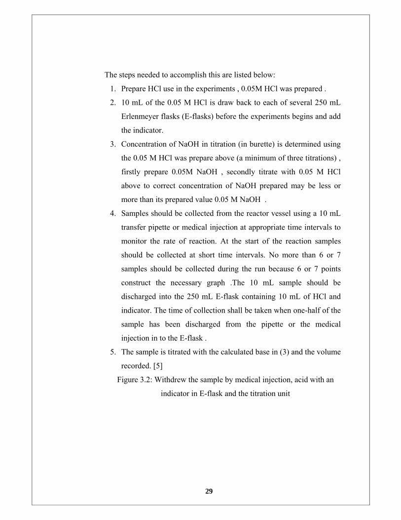
The steps needed to accomplish this are listed below:
1. Prepare HCl use in the experiments , 0.05M HCl was prepared .
2. 10 mL of the 0.05 M HCl is draw back to each of several 250 mL
Erlenmeyer flasks (E-flasks) before the experiments begins and add
the indicator.
3. Concentration of NaOH in titration (in burette) is determined using
the 0.05 M HCl was prepare above (a minimum of three titrations) ,
firstly prepare 0.05M NaOH , secondly titrate with 0.05 M HCl
above to correct concentration of NaOH prepared may be less or
more than its prepared value 0.05 M NaOH .
4. Samples should be collected from the reactor vessel using a 10 mL
transfer pipette or medical injection at appropriate time intervals to
monitor the rate of reaction. At the start of the reaction samples
should be collected at short time intervals. No more than 6 or 7
samples should be collected during the run because 6 or 7 points
construct the necessary graph .The 10 mL sample should be
discharged into the 250 mL E-flask containing 10 mL of HCl and
indicator. The time of collection shall be taken when one-half of the
sample has been discharged from the pipette or the medical
injection in to the E-flask .
5. The sample is titrated with the calculated base in (3) and the volume
recorded. [5]
Figure 3.2: Withdrew the sample by medical injection, acid with an
indicator in E-flask and the titration unit
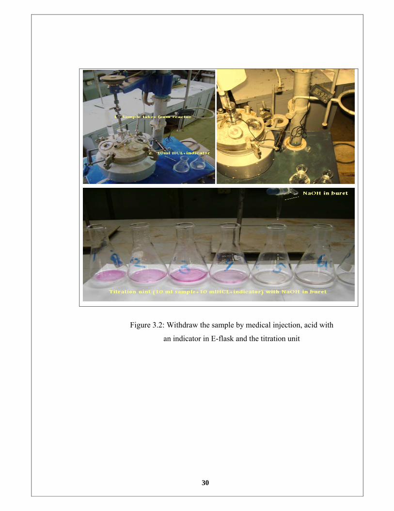
30
Figure 3.2: Withdraw the sample by medical injection, acid with
an indicator in E-flask and the titration unit
31
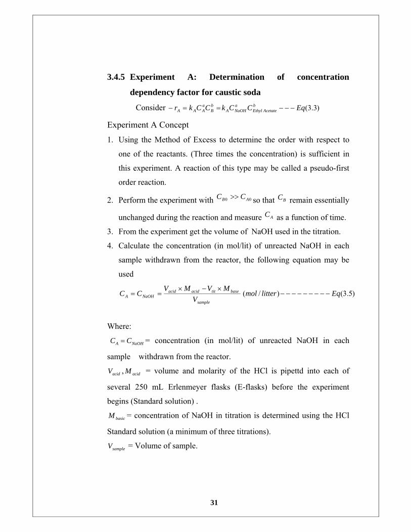
3.4.5 Experiment A: Determination of concentration
dependency factor for caustic soda
Consider )3.3(EqCCkCCkr bAcetateEthyl
aNaOHA
bB
aAAA −−−==−
Experiment A Concept
1. Using the Method of Excess to determine the order with respect to
one of the reactants. (Three times the concentration) is sufficient in
this experiment. A reaction of this type may be called a pseudo-first
order reaction.
2. Perform the experiment with 00 AB CC >> so that BC remain essentially
unchanged during the reaction and measure AC as a function of time.
3. From the experiment get the volume of NaOH used in the titration.
4. Calculate the concentration (in mol/lit) of unreacted NaOH in each
sample withdrawn from the reactor, the following equation may be
used
)5.3()/( EqlittermolV
MVMVCC
sample
basetitacidacidNaOHA −−−−−−−−−
×−×==
Where:
NaOHA CC = = concentration (in mol/lit) of unreacted NaOH in each
sample withdrawn from the reactor.
acidV , acidM = volume and molarity of the HCl is pipettd into each of
several 250 mL Erlenmeyer flasks (E-flasks) before the experiment
begins (Standard solution) .
basicM = concentration of NaOH in titration is determined using the HCl
Standard solution (a minimum of three titrations).
sampleV = Volume of sample.
32
Table 3.1: Experiment A Concept Concentration of unreacted NaOH
Time , second 0t 1t 2t 3t 4t nt
Concentration of NaOHC (mol/lit) 0AC 1AC 2AC 3AC 4AC AnC
5. Using differential method to evaluate aandk ′ because one might
get
a fractional order.
)6.3(EqCkCCkCCkr aA
aA
bBA
bB
aAAA −−−−−−−−−−−−′===−
)7.3(0 EqCkCkk bBA
bBA −−−−−−−−−−−−−−−−−−−−≈=′
)8.3()ln()ln()ln( EqCakr AA −−−−−−−−−−−−−−−−+′=−
6. Used method of finite difference to calculate )( Ar− or )(dtdC A−
( 2.6.2 , Eqs( 2.27 to 2.29))
7. Use Excel program to Plot log-log graph for )( Ar− vs AC
and Trend (Line, power) to get aandk ′
Experiment A Procedure (Three Batches) :
Isothermal operation at C07.37
Procedure:
1. 0.05 M HCl was prepared and used in the experiment (Standard
acid solution) ,10 mL of it is pipetted into each of several 250 mL
Erlenmeyer flasks (E-flasks) before the experiment began .
2. Concentration of NaOH in titration (in burette) is determined
using the 0.05 M HCl was prepared above (a minimum of three
titrations) , firstly prepare 0.05M NaOH , secondly titrate it with
0.05 M HCl above to correct concentration of NaOH prepared
may be less or more than its prepared value 0.05 M NaOH in
Table(3.2) .
)9.3(EqMVMV basicbaseacidacid −−−−−−−−−−−−−−−−−−−−−×=×
33
Table 3.2: Experiment A acid base titration Standard acid solution Measured base solution
NO(titrations) acidV (ml) acidM (mol/lit) baseV (ml) baseM (mol/lit) Average baseM (mol/lit)
1 10 0.05 10.35 0.048309
2 10 0.05 10.30 0.048544
3 10 0.05 10.25 0.048780
0.048544
3. In the reactor, mix 0.5 liter of the 0.1M caustic soda solution with
0.5 liter of the 0.3M ethyl acetate solution at an arbitrary time (t =
0) at C07.37 switch on the stirrer immediately and set it to an
intermediate speed to avoid splashing.
4. Start the timer as soon as you start mixing the reactants.
5. After a certain time interval, use a medical injection to withdraw
10ml sample from the reactor, and immediately quench it with
10ml of excess 0.05M hydrochloric acid (You should have the
quenching acid sample ready before taking the sample from the
reactor) .
6. Add 2 - 3 drops of phenolphthalein to the quenched sample and
back titrate with 0.048544 M NaOH solution until the end point is
detected (in this case a stable pink color) .
7. Record the amount of NaOH used in the titration (V titration.).
8. Repeat steps (5) - (7) every 1 minute for the samples. Take a total
of 6-7samples making sure that you record the time for each new
sample.
9. Calculate experiment A batch (I) volume of NaOH used in the
titration, the results are shown in (Table 3.3).
34
Table 3.3: Experiment A batch (I) volume of NaOH used in the
titration
Sample Time (s) Initial Burette
reading (ml)
Final Burette
Reading(ml)
Volume NaOH
used in Titration[Final-
Initial](ml)
0 0 0 0 0
1 60 10.3 19.25 8.95
2 120 19.25 29.1 9.85
3 180 29.1 39.15 10.05
4 240 39.15 49.30 10.15
5 300 0 10.2 10.2
6 360 10.2 20.45 10.25
10. Calculate the concentration (in mol/lit) of un reacted NaOH in
each sample withdrawn from the reactor in (Table 3.3) by use Eq
(3.5) , The results are shown in (Table 3.4)
10048544.005.010 ×−×
=×−×
= tit
sample
basetitacidacidNaOH
VV
MVMVC
[ ] 1.010
048544.0005.0100 =
×−×==tNaOHC
[ ] 0065531.010
048544.095.805.01060 =
×−×==tNaOHC
[ ] 0.002184210
048544.085.905.010120 =
×−×==tNaOHC
[ ] 0.001213310
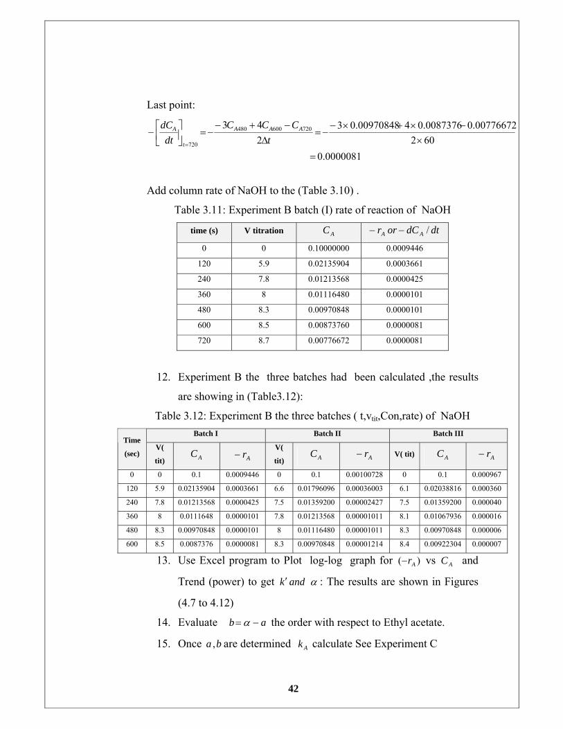
048544.005.1005.010180 =
×−×==tNaOHC
[ ] 0.000727810
048544.015.1005.010240 =
×−×==tNaOHC
[ ] 0.000485110
048544.02.1005.010300 =
×−×==tNaOHC
[ ] 0.000242410
048544.025.1005.010360 =
×−×==tNaOHC
Add column un reacted NaOH to the (Table 3.3) :
35
Table 3.4: Experiment A batch (I) Concentration of unreacted NaOH
Sample # Time
(s)
Volume NaOH used in titration
(ml) Un reacted NaOH(mol/lit)
0 0 0 0.1
1 60 7.95 0.00655312
2 120 9.85 0.00218416
3 180 10.05 0.00121328
4 240 10.15 0.00072784
5 300 10.2 0.00048512
6 360 10.25 0.00024240
11. Use the Numerical Methods (finite difference) to calculate
)( Ar− or )(dtdC A− .( 2.6.2 , Eqs 2.27 to 2.29) ,The results are shown
in(Table 3.5)
Initial point:
0.0022998
60200218416.000655312.041.03
243 120600
0
=
×−×+×−
−=∆
−+−−=⎥⎦
⎤⎢⎣
⎡−= t
CCCdt
dC AAA
t
A
Interior points:
0.0008151602
)0.10000000.0021842(2
0120
60
=×−
−=∆−
−=⎥⎦⎤
⎢⎣⎡−
= tCC
dtdC AA
t
A
0.0000445602
)0.00655310.0012133(2
60180
120
=×−
−=∆−
−=⎥⎦⎤
⎢⎣⎡−
= tCC
dtdC AA
t
A
0.0000121602
)0.00218420.0007278(2
120240
180
=×−
−=∆−
−=⎥⎦⎤
⎢⎣⎡−
= tCC
dtdC AA
t
A
0.0000061602
)0.00121330.0004851(2
180300
240
=×−
−=∆−
−=⎥⎦⎤
⎢⎣⎡−
= tCC
dtdC AA
t
A
0.0000040602
)0.00072780.0002424(2
240360
300
=×−
−=∆−
−=⎥⎦⎤
⎢⎣⎡−
= tCC
dtdC AA
t
A
36
Last point:
0.0000040602
0.00024240.000485140.00072783243 360300240
360
=
×−×+×−
−=∆
−+−−=⎥⎦
⎤⎢⎣⎡−
= tCCC
dtdC AAA
t
A
Add column of the rate of reaction NaOH to the (Table 3.4) .
Table 3.5: Experiment A batch (I) rate of reaction of NaOH
time (s) V titration AC dtdCorr AA /−−
0 0 0.1000000 0.0022998
60 8.95 0.0065531 0.0008151
120 9.85 0.0021842 0.0000445
180 10.05 0.0012133 0.0000121
240 10.15 0.0007278 0.0000061
300 10.2 0.0004851 0.0000040
360 10.25 0.0002424 0.0000040
12. Experiment A the three batches had been calculated, the results
are showing in (Table 3.6). Table 3.6: Experiment A the three batches ( t,vtit,Con,rate) of NaOH
Batch I Batch II Batch III Time
(sec) V(
tit) AC Ar−
V(
tit) AC Ar− V(
tit) AC Ar−
0 0 0.1000000 0.0022998 0 0.1 0.002278 0 0.10000000 0.002275
60 8.95 0.0065531 0.0008151 8.8 0.00728128 0.000813 8.75 0.00752400 0.000807
120 9.85 0.0021842 0.0000445 9.8 0.00242688 0.000097 9.65 0.00315504 0.000109
180 10.05 0.0012133 0.0000121 10 0.00145600 0.000028 10.1 0.00097056 0.000040
240 10.15 0.0007278 0.0000061 10.15 0.00072784 0.000016 10.15 0.00072784 0.000008
300 10.2 0.0004851 0.0000040 10.2 0.00048512 0.000008 10.2 0.00048512 0.000008
360 10.25 0.0002424 0.0000040 10.25 0.0002424 0.000004045 10.25 0.00024 0.000004005
13. Use Excel program to Plot log-log graph between )( Ar− vs AC
and Trend ( power) to get aandk ′ : The results are shown in
Figures (4.1 to 4.6)
37
3.4.6 Experiment B: Determination of concentration
dependency factor for Ethyl Acetate.
Consider )3.3(EqCCkCCkr bAcetateEthyl
aNaOHA
bB
aAAA −−−==−
Experiment B Concept
1. To determine the reaction order overall. This can be done by running
the experiment as a batch reactor with equal initial concentrations of
both reactants. A minimum of three batch experiments should be run
with equal concentrations of reactants, one at the same temperature of
Experiment A.
2. Perform the experiment with 00 BA CC = and measure AC as a function
of time.
3. From the experiment get the volume of NaOH used in the titration .
4. Calculate the concentration (in mol/lit) of unreacted NaOH in each
sample withdrawn from the reactor, the following equation may be
used
)5.3()/( EqlittermolV
MVMVCC
sample
basetitacidacidNaOHA −−−−−−−−−
×−×==
Where:
NaOHA CC = = concentration (in mol/lit) of unreacted NaOH in each
sample withdrawn from the reactor.
acidV , acidM = volume and molarity of the HCl is pipettd into each of
several 250 mL Erlenmeyer flasks (E-flasks) before the experiment
begins (Standard solution) .
basicM = concentration of NaOH in titration is determined using the
HCl Standard solution (a minimum of three titrations).
sampleV = Volume of sample.
38
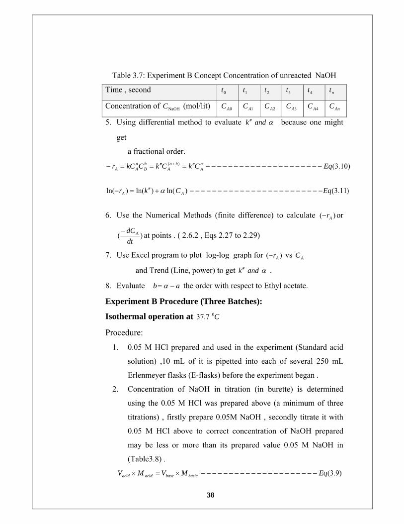
Table 3.7: Experiment B Concept Concentration of unreacted NaOH
Time , second 0t 1t 2t 3t 4t nt
Concentration of NaOHC (mol/lit) 0AC 1AC 2AC 3AC 4AC AnC
5. Using differential method to evaluate αandk ′′ because one might
get
a fractional order.
)10.3()( EqCkCkCkCr Aba
AbB
aAA −−−−−−−−−−−−−−−−−−−−−′′=′′==− + α
)11.3()ln()ln()ln( EqCkr AA −−−−−−−−−−−−−−−−−−−−−−−−+′′=− α
6. Use the Numerical Methods (finite difference) to calculate )( Ar− or
)(dtdCA− at points . ( 2.6.2 , Eqs 2.27 to 2.29)
7. Use Excel program to plot log-log graph for )( Ar− vs AC
and Trend (Line, power) to get αandk ′′ .
8. Evaluate ab −= α the order with respect to Ethyl acetate.
Experiment B Procedure (Three Batches):
Isothermal operation at C07.37
Procedure:
1. 0.05 M HCl prepared and used in the experiment (Standard acid
solution) ,10 mL of it is pipetted into each of several 250 mL
Erlenmeyer flasks (E-flasks) before the experiment began .
2. Concentration of NaOH in titration (in burette) is determined
using the 0.05 M HCl was prepared above (a minimum of three
titrations) , firstly prepare 0.05M NaOH , secondly titrate it with
0.05 M HCl above to correct concentration of NaOH prepared
may be less or more than its prepared value 0.05 M NaOH in
(Table3.8) .
)9.3(EqMVMV basicbaseacidacid −−−−−−−−−−−−−−−−−−−−−×=×

39
Table 3.8: Experiment B acid base titration Standard acid solution Measured base solution
NO(titrations) acidV (ml) acidM (mol/lit) baseV (ml) baseM (mol/lit) Average baseM (mol/lit)
1 10 0.05 10.30 0.048544
2 10 0.05 10.35 0.048309
3 10 0.05 10.25 0.048780
0.048544
3. In the reactor, mix 0.5 liter of the 0.1M caustic soda solution with
0.5 liter of the 0.1M ethyl acetate solution at an arbitrary time (t =
0) at C07.37 . Switch on the stirrer immediately and set it to an
intermediate speed to avoid splashing.
4. Start the timer as soon as you start mixing the reactants.
5. After a certain time interval, use a pipette or medical injection to
withdraw 10ml sample from the reactor, and immediately quench
it with 10ml of excess 0.05M hydrochloric acid (You should have
the quenching acid sample ready before taking the sample from
the reactor) .
6. Add 2 - 3 drops of phenolphthalein to the quenched sample and
back titrate with 0.048544 M NaOH solution until the end point is
detected (in this case a stable pink color) .
7. Record the amount of NaOH used in the titration (V titration.).
8. Repeat steps (5) - (7) every 2 minute for the samples. Take a total
of 6-7samples making sure that you record the time for each new
sample
9. Calculate experiment B batch (I) volume of NaOH used in the
titration ,The results are shown in (Table 3.9)
40
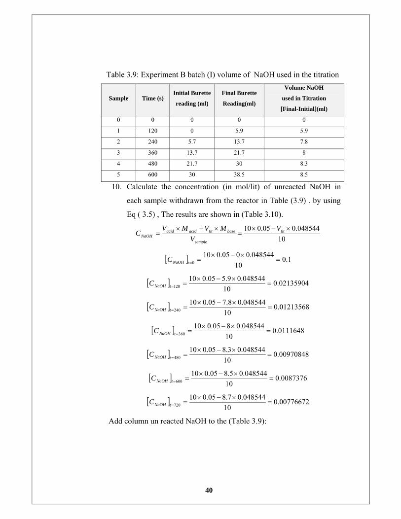
Table 3.9: Experiment B batch (I) volume of NaOH used in the titration
Sample Time (s) Initial Burette
reading (ml)
Final Burette
Reading(ml)
Volume NaOH
used in Titration
[Final-Initial](ml)
0 0 0 0 0
1 120 0 5.9 5.9
2 240 5.7 13.7 7.8
3 360 13.7 21.7 8
4 480 21.7 30 8.3
5 600 30 38.5 8.5
10. Calculate the concentration (in mol/lit) of unreacted NaOH in
each sample withdrawn from the reactor in Table (3.9) . by using
Eq ( 3.5) , The results are shown in (Table 3.10).
10048544.005.010 ×−×
=×−×
= tit
sample
basetitacidacidNaOH
VV
MVMVC
[ ] 1.010
048544.0005.0100 =
×−×==tNaOHC
[ ] 0.0213590410
048544.09.505.010120 =
×−×==tNaOHC
[ ] 0.0121356810
048544.08.705.010240 =
×−×==tNaOHC
[ ] 0.011164810
048544.0805.010360 =
×−×==tNaOHC
[ ] 0.0097084810
048544.03.805.010480 =
×−×==tNaOHC
[ ] 0.008737610
048544.05.805.010600 =
×−×==tNaOHC
[ ] 0.0077667210
048544.07.805.010720 =
×−×==tNaOHC
Add column un reacted NaOH to the (Table 3.9):
41
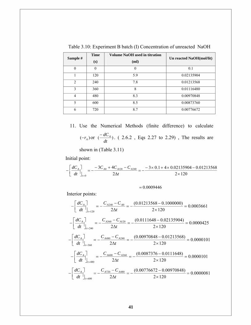
Table 3.10: Experiment B batch (I) Concentration of unreacted NaOH
Sample # Time
(s)
Volume NaOH used in titration
(ml) Un reacted NaOH(mol/lit)
0 0 0 0.1
1 120 5.9 0.02135904
2 240 7.8 0.01213568
3 360 8 0.01116480
4 480 8.3 0.00970848
5 600 8.5 0.00873760
6 720 8.7 0.00776672
11. Use the Numerical Methods (finite difference) to calculate
)( Ar− or )(dtdCA− . ( 2.6.2 , Eqs 2.27 to 2.29) , The results are
shown in (Table 3.11)
Initial point:
0.0009446
12020.012135680.0213590441.03
243 2401200
0
=
×−×+×−
−=∆
−+−−=⎥⎦
⎤⎢⎣
⎡−= t
CCCdt
dC AAA
t
A
Interior points:
0.00036611202
)0.10000000.01213568(2
0240
120
=×−
−=∆−
−=⎥⎦⎤
⎢⎣⎡−
= tCC
dtdC AA
t
A
0.00004251202
)0.021359040.0111648(2
120360
240
=×−
−=∆−
−=⎥⎦⎤
⎢⎣⎡−
= tCC
dtdC AA
t
A
0.00001011202
)0.012135680.00970848(2
240480
360
=×−
−=∆−
−=⎥⎦⎤
⎢⎣⎡−
= tCC
dtdC AA
t
A
0.00001011202
)0.01116480.0087376(2
360600
480
=×−
−=∆−
−=⎥⎦⎤
⎢⎣⎡−
= tCC
dtdC AA
t
A
0.00000811202
)0.009708480.00776672(2
480720
600
=×−
−=∆−
−=⎥⎦⎤
⎢⎣⎡−
= tCC
dtdC AA
t
A
42
Last point:
0.0000081602
0.007766720.008737640.009708483243 720600480
720
=
×−×+×−
−=∆
−+−−=⎥⎦
⎤⎢⎣
⎡−= t
CCCdt
dC AAA
t
A
Add column rate of NaOH to the (Table 3.10) .
Table 3.11: Experiment B batch (I) rate of reaction of NaOH
time (s) V titration AC dtdCorr AA /−−
0 0 0.10000000 0.0009446
120 5.9 0.02135904 0.0003661
240 7.8 0.01213568 0.0000425
360 8 0.01116480 0.0000101
480 8.3 0.00970848 0.0000101
600 8.5 0.00873760 0.0000081
720 8.7 0.00776672 0.0000081
12. Experiment B the three batches had been calculated ,the results
are showing in (Table3.12):
Table 3.12: Experiment B the three batches ( t,vtit,Con,rate) of NaOH Batch I Batch II Batch III
Time
(sec) V(
tit) AC Ar−
V(
tit) AC Ar− V( tit) AC Ar−
0 0 0.1 0.0009446 0 0.1 0.00100728 0 0.1 0.000967
120 5.9 0.02135904 0.0003661 6.6 0.01796096 0.00036003 6.1 0.02038816 0.000360
240 7.8 0.01213568 0.0000425 7.5 0.01359200 0.00002427 7.5 0.01359200 0.000040
360 8 0.0111648 0.0000101 7.8 0.01213568 0.00001011 8.1 0.01067936 0.000016
480 8.3 0.00970848 0.0000101 8 0.01116480 0.00001011 8.3 0.00970848 0.000006
600 8.5 0.0087376 0.0000081 8.3 0.00970848 0.00001214 8.4 0.00922304 0.000007
13. Use Excel program to Plot log-log graph for )( Ar− vs AC and
Trend (power) to get αandk ′ : The results are shown in Figures
(4.7 to 4.12)
14. Evaluate ab −= α the order with respect to Ethyl acetate.
15. Once ba , are determined Ak calculate See Experiment C
43
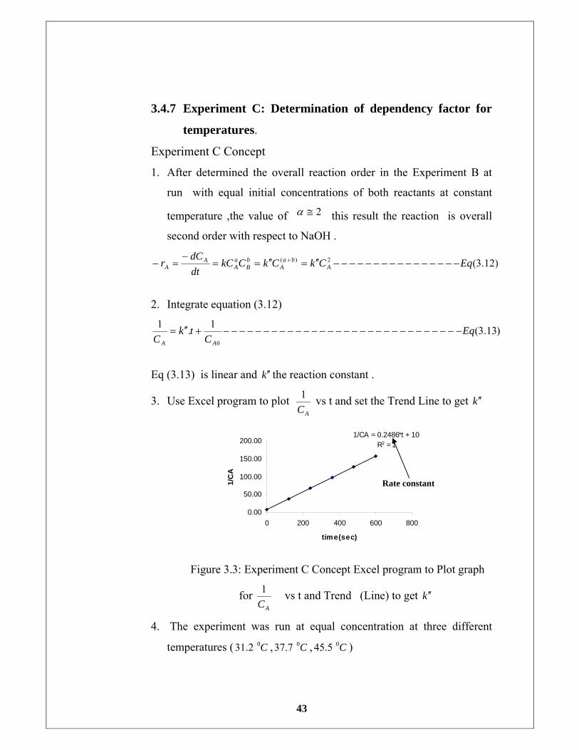
3.4.7 Experiment C: Determination of dependency factor for
temperatures.
Experiment C Concept
1. After determined the overall reaction order in the Experiment B at
run with equal initial concentrations of both reactants at constant
temperature ,the value of 2≅α this result the reaction is overall
second order with respect to NaOH .
)12.3(2)( EqCkCkCkCdtdC
r Aba
AbB
aA
AA −−−−−−−−−−−−−−−−′′=′′==
−=− +
2. Integrate equation (3.12)
)13.3(1.1
0
EqC
tkC AA
−−−−−−−−−−−−−−−−−−−−−−−−−−−−−−+′′=
Eq (3.13) is linear and k ′′ the reaction constant .
3. Use Excel program to plot AC
1 vs t and set the Trend Line to get k ′′
1/CA = 0.2486*t + 10R2 = 1
0.00
50.00
100.00
150.00
200.00
0 200 400 600 800
time(sec)
1/C
A
Figure 3.3: Experiment C Concept Excel program to Plot graph
for AC
1 vs t and Trend (Line) to get k ′′
4. The experiment was run at equal concentration at three different
temperatures ( C02.31 , C07.37 , C05.45 )
Rate constant
44
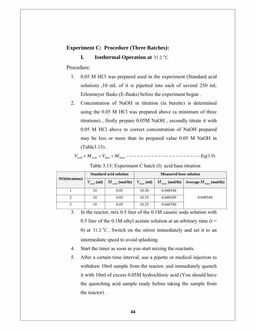
Experiment C: Procedure (Three Batches):
I. Isothermal Operation at C02.31
Procedure:
1. 0.05 M HCl was prepared used in the experiment (Standard acid
solution) ,10 mL of it is pipetted into each of several 250 mL
Erlenmeyer flasks (E-flasks) before the experiment began .
2. Concentration of NaOH in titration (in burette) is determined
using the 0.05 M HCl was prepared above (a minimum of three
titrations) , firstly prepare 0.05M NaOH , secondly titrate it with
0.05 M HCl above to correct concentration of NaOH prepared
may be less or more than its prepared value 0.05 M NaOH in
(Table3.13) .
)9.3(EqMVMV basicbaseacidacid −−−−−−−−−−−−−−−−−−−−−×=×
Table 3.13: Experiment C batch (I) acid base titration Standard acid solution Measured base solution
NO(titrations) acidV (ml) acidM (mol/lit) baseV (ml) baseM (mol/lit) Average baseM (mol/lit)
1 10 0.05 10.30 0.048544
2 10 0.05 10.35 0.048309
3 10 0.05 10.25 0.048780
0.048544
3. In the reactor, mix 0.5 liter of the 0.1M caustic soda solution with
0.5 liter of the 0.1M ethyl acetate solution at an arbitrary time (t =
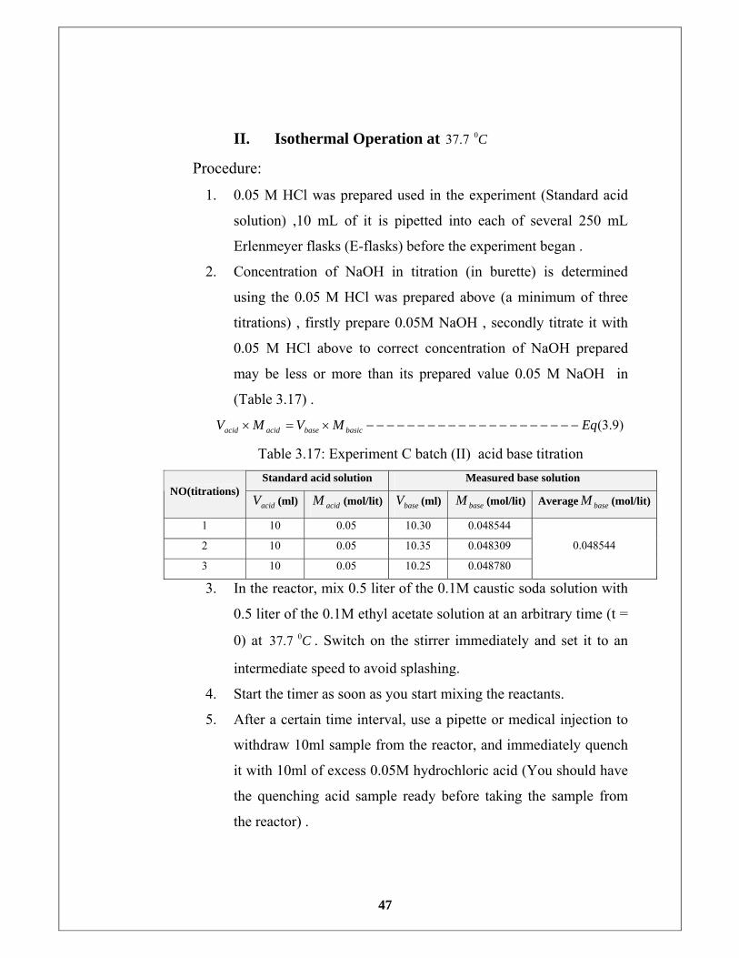
0) at C02.31 . Switch on the stirrer immediately and set it to an
intermediate speed to avoid splashing.
4. Start the timer as soon as you start mixing the reactants.
5. After a certain time interval, use a pipette or medical injection to
withdraw 10ml sample from the reactor, and immediately quench
it with 10ml of excess 0.05M hydrochloric acid (You should have
the quenching acid sample ready before taking the sample from
the reactor) .
45
6. Add 2 - 3 drops of phenolphthalein to the quenched sample and
back titrate with 0.048544 M NaOH solution until the end point is
detected (in this case a stable pink color) .
7. Record the amount of NaOH used in the titration (V titration.).
8. Repeat steps (5) - (7) every 2 minute for the samples. Take a total
of 6-7samples making sure that you record the time for each new
sample.
9. Calculation Experiment C batch (I) at C02.31 . The results are
shown in (Table 3.14)
Table 3.14: Experiment C batch (I) volume of NaOH used in the
titration
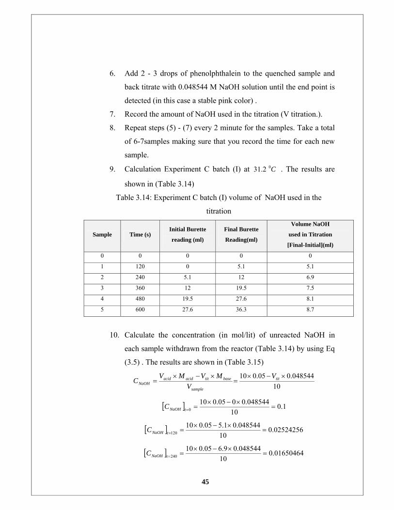
10. Calculate the concentration (in mol/lit) of unreacted NaOH in
each sample withdrawn from the reactor (Table 3.14) by using Eq
(3.5) . The results are shown in (Table 3.15)
10048544.005.010 ×−×
=×−×
= tit
sample
basetitacidacidNaOH
VV
MVMVC
[ ] 1.010
048544.0005.0100 =
×−×==tNaOHC
[ ] 0.0252425610
048544.01.505.010120 =
×−×==tNaOHC
[ ] 0.0165046410
048544.09.605.010240 =
×−×==tNaOHC
Sample Time (s) Initial Burette
reading (ml)
Final Burette
Reading(ml)
Volume NaOH
used in Titration
[Final-Initial](ml)
0 0 0 0 0
1 120 0 5.1 5.1
2 240 5.1 12 6.9
3 360 12 19.5 7.5
4 480 19.5 27.6 8.1
5 600 27.6 36.3 8.7
46
[ ] 0.01359210
048544.05.705.010360 =
×−×==tNaOHC
[ ] 0.0106793610
048544.01.805.010480 =
×−×==tNaOHC
[ ] 0.0077667210
048544.07.805.010600 =
×−×==tNaOHC
Add column un reacted NaOH to the (Table 3.14) :
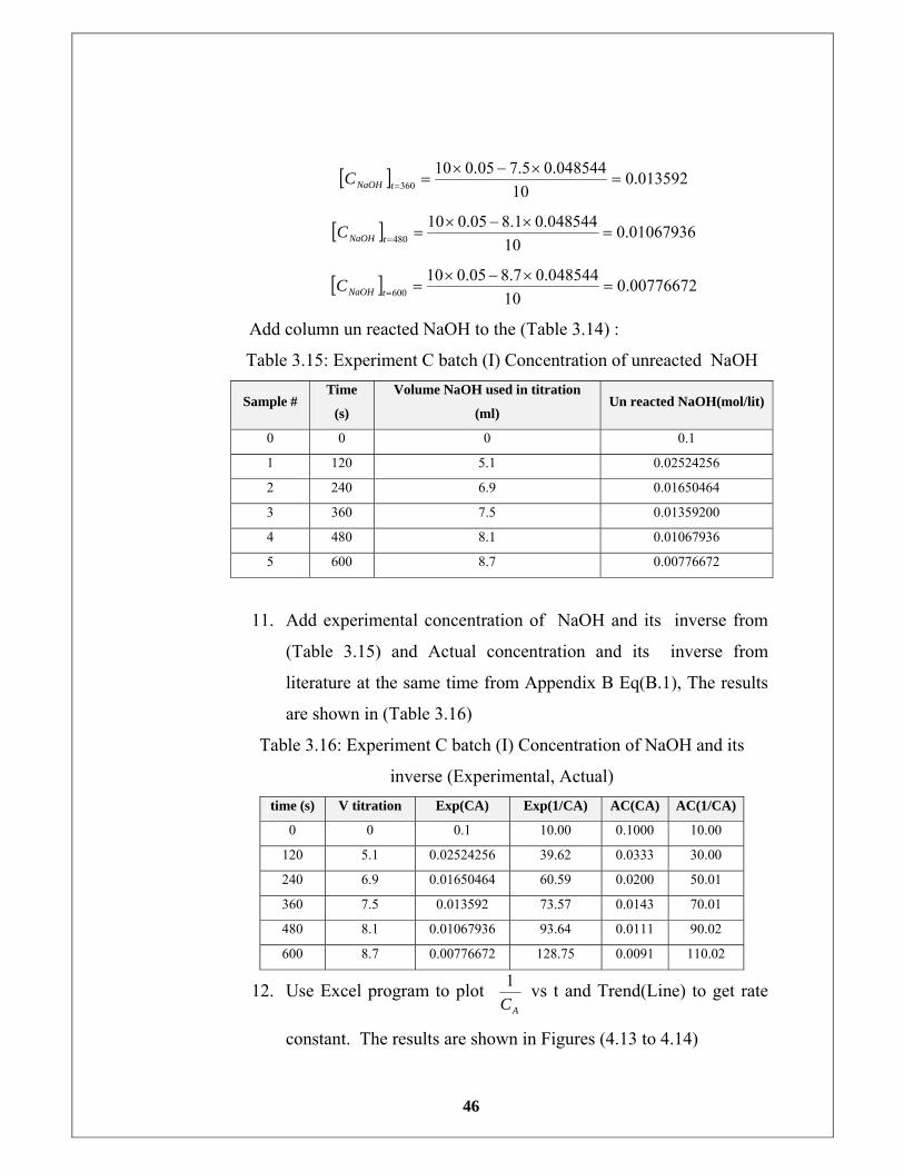
Table 3.15: Experiment C batch (I) Concentration of unreacted NaOH
Sample # Time
(s)
Volume NaOH used in titration
(ml) Un reacted NaOH(mol/lit)
0 0 0 0.1
1 120 5.1 0.02524256
2 240 6.9 0.01650464
3 360 7.5 0.01359200
4 480 8.1 0.01067936
5 600 8.7 0.00776672
11. Add experimental concentration of NaOH and its inverse from
(Table 3.15) and Actual concentration and its inverse from
literature at the same time from Appendix B Eq(B.1), The results
are shown in (Table 3.16)
Table 3.16: Experiment C batch (I) Concentration of NaOH and its
inverse (Experimental, Actual) time (s) V titration Exp(CA) Exp(1/CA) AC(CA) AC(1/CA)
0 0 0.1 10.00 0.1000 10.00
120 5.1 0.02524256 39.62 0.0333 30.00
240 6.9 0.01650464 60.59 0.0200 50.01
360 7.5 0.013592 73.57 0.0143 70.01
480 8.1 0.01067936 93.64 0.0111 90.02
600 8.7 0.00776672 128.75 0.0091 110.02
12. Use Excel program to plot AC
1 vs t and Trend(Line) to get rate
constant. The results are shown in Figures (4.13 to 4.14)
47
II. Isothermal Operation at C07.37
Procedure:
1. 0.05 M HCl was prepared used in the experiment (Standard acid
solution) ,10 mL of it is pipetted into each of several 250 mL
Erlenmeyer flasks (E-flasks) before the experiment began .
2. Concentration of NaOH in titration (in burette) is determined
using the 0.05 M HCl was prepared above (a minimum of three
titrations) , firstly prepare 0.05M NaOH , secondly titrate it with
0.05 M HCl above to correct concentration of NaOH prepared
may be less or more than its prepared value 0.05 M NaOH in
(Table 3.17) .
)9.3(EqMVMV basicbaseacidacid −−−−−−−−−−−−−−−−−−−−−×=×
Table 3.17: Experiment C batch (II) acid base titration Standard acid solution Measured base solution
NO(titrations) acidV (ml) acidM (mol/lit) baseV (ml) baseM (mol/lit) Average baseM (mol/lit)
1 10 0.05 10.30 0.048544
2 10 0.05 10.35 0.048309
3 10 0.05 10.25 0.048780
0.048544
3. In the reactor, mix 0.5 liter of the 0.1M caustic soda solution with
0.5 liter of the 0.1M ethyl acetate solution at an arbitrary time (t =
0) at C07.37 . Switch on the stirrer immediately and set it to an
intermediate speed to avoid splashing.
4. Start the timer as soon as you start mixing the reactants.
5. After a certain time interval, use a pipette or medical injection to
withdraw 10ml sample from the reactor, and immediately quench
it with 10ml of excess 0.05M hydrochloric acid (You should have
the quenching acid sample ready before taking the sample from
the reactor) .
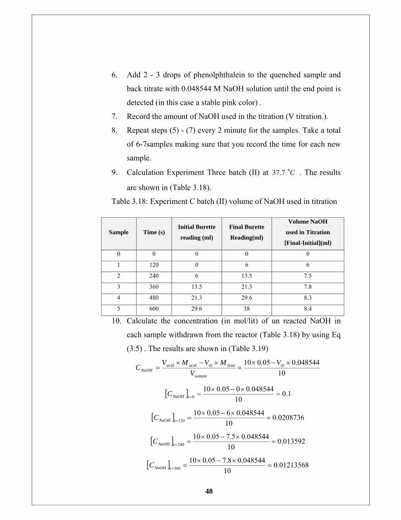
48
6. Add 2 - 3 drops of phenolphthalein to the quenched sample and
back titrate with 0.048544 M NaOH solution until the end point is
detected (in this case a stable pink color) .
7. Record the amount of NaOH used in the titration (V titration.).
8. Repeat steps (5) - (7) every 2 minute for the samples. Take a total
of 6-7samples making sure that you record the time for each new
sample.
9. Calculation Experiment Three batch (II) at C07.37 . The results
are shown in (Table 3.18).
Table 3.18: Experiment C batch (II) volume of NaOH used in titration
10. Calculate the concentration (in mol/lit) of un reacted NaOH in
each sample withdrawn from the reactor (Table 3.18) by using Eq
(3.5) . The results are shown in (Table 3.19)
10048544.005.010 ×−×
=×−×
= tit
sample
basetitacidacidNaOH
VV
MVMVC
[ ] 1.010
048544.0005.0100 =
×−×==tNaOHC
[ ] 0.020873610
048544.0605.010120 =
×−×==tNaOHC
[ ] 0.01359210
048544.05.705.010240 =
×−×==tNaOHC
[ ] 0.0121356810
048544.08.705.010360 =
×−×==tNaOHC
Sample Time (s) Initial Burette
reading (ml)
Final Burette
Reading(ml)
Volume NaOH
used in Titration
[Final-Initial](ml)
0 0 0 0 0
1 120 0 6 6
2 240 6 13.5 7.5
3 360 13.5 21.3 7.8
4 480 21.3 29.6 8.3
5 600 29.6 38 8.4
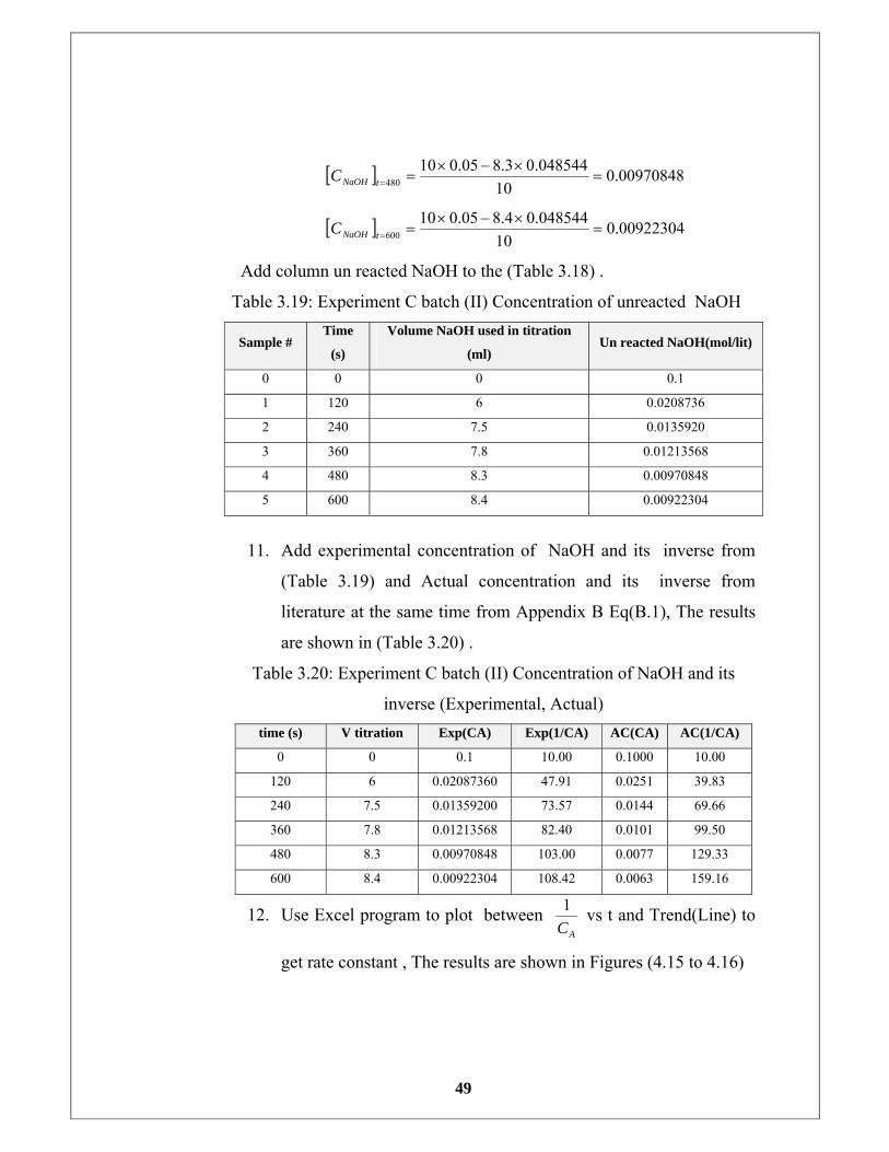
49
[ ] 0.0097084810
048544.03.805.010480 =
×−×==tNaOHC
[ ] 0.0092230410
048544.04.805.010600 =
×−×==tNaOHC
Add column un reacted NaOH to the (Table 3.18) .
Table 3.19: Experiment C batch (II) Concentration of unreacted NaOH
Sample # Time
(s)
Volume NaOH used in titration
(ml) Un reacted NaOH(mol/lit)
0 0 0 0.1
1 120 6 0.0208736
2 240 7.5 0.0135920
3 360 7.8 0.01213568
4 480 8.3 0.00970848
5 600 8.4 0.00922304
11. Add experimental concentration of NaOH and its inverse from
(Table 3.19) and Actual concentration and its inverse from
literature at the same time from Appendix B Eq(B.1), The results
are shown in (Table 3.20) .
Table 3.20: Experiment C batch (II) Concentration of NaOH and its
inverse (Experimental, Actual) time (s) V titration Exp(CA) Exp(1/CA) AC(CA) AC(1/CA)
0 0 0.1 10.00 0.1000 10.00
120 6 0.02087360 47.91 0.0251 39.83
240 7.5 0.01359200 73.57 0.0144 69.66
360 7.8 0.01213568 82.40 0.0101 99.50
480 8.3 0.00970848 103.00 0.0077 129.33
600 8.4 0.00922304 108.42 0.0063 159.16
12. Use Excel program to plot between AC
1 vs t and Trend(Line) to
get rate constant , The results are shown in Figures (4.15 to 4.16)
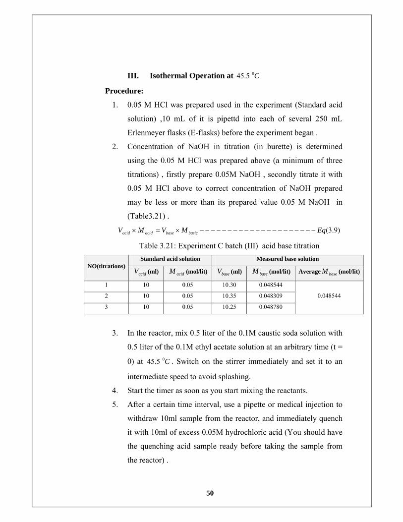
50
III. Isothermal Operation at C05.45
Procedure:
1. 0.05 M HCl was prepared used in the experiment (Standard acid
solution) ,10 mL of it is pipettd into each of several 250 mL
Erlenmeyer flasks (E-flasks) before the experiment began .
2. Concentration of NaOH in titration (in burette) is determined
using the 0.05 M HCl was prepared above (a minimum of three
titrations) , firstly prepare 0.05M NaOH , secondly titrate it with
0.05 M HCl above to correct concentration of NaOH prepared
may be less or more than its prepared value 0.05 M NaOH in
(Table3.21) .
)9.3(EqMVMV basicbaseacidacid −−−−−−−−−−−−−−−−−−−−−×=×
Table 3.21: Experiment C batch (III) acid base titration Standard acid solution Measured base solution
NO(titrations) acidV (ml) acidM (mol/lit) baseV (ml) baseM (mol/lit) Average baseM (mol/lit)
1 10 0.05 10.30 0.048544
2 10 0.05 10.35 0.048309
3 10 0.05 10.25 0.048780
0.048544
3. In the reactor, mix 0.5 liter of the 0.1M caustic soda solution with
0.5 liter of the 0.1M ethyl acetate solution at an arbitrary time (t =
0) at C05.45 . Switch on the stirrer immediately and set it to an
intermediate speed to avoid splashing.
4. Start the timer as soon as you start mixing the reactants.
5. After a certain time interval, use a pipette or medical injection to
withdraw 10ml sample from the reactor, and immediately quench
it with 10ml of excess 0.05M hydrochloric acid (You should have
the quenching acid sample ready before taking the sample from
the reactor) .
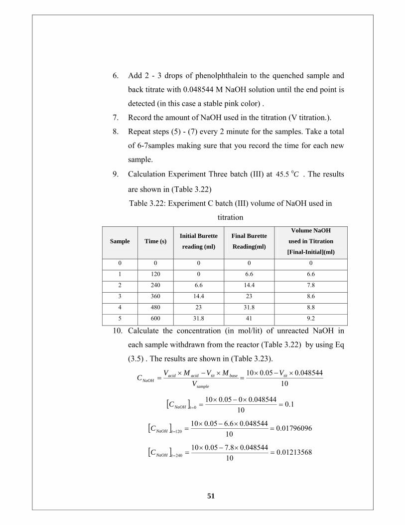
51
6. Add 2 - 3 drops of phenolphthalein to the quenched sample and
back titrate with 0.048544 M NaOH solution until the end point is
detected (in this case a stable pink color) .
7. Record the amount of NaOH used in the titration (V titration.).
8. Repeat steps (5) - (7) every 2 minute for the samples. Take a total
of 6-7samples making sure that you record the time for each new
sample.
9. Calculation Experiment Three batch (III) at C05.45 . The results
are shown in (Table 3.22)
Table 3.22: Experiment C batch (III) volume of NaOH used in
titration
Sample Time (s) Initial Burette
reading (ml)
Final Burette
Reading(ml)
Volume NaOH
used in Titration
[Final-Initial](ml)
0 0 0 0 0
1 120 0 6.6 6.6
2 240 6.6 14.4 7.8
3 360 14.4 23 8.6
4 480 23 31.8 8.8
5 600 31.8 41 9.2
10. Calculate the concentration (in mol/lit) of unreacted NaOH in
each sample withdrawn from the reactor (Table 3.22) by using Eq
(3.5) . The results are shown in (Table 3.23).
10048544.005.010 ×−×
=×−×
= tit
sample
basetitacidacidNaOH
VV
MVMVC
[ ] 1.010
048544.0005.0100 =
×−×==tNaOHC
[ ] 0.0179609610
048544.06.605.010120 =
×−×==tNaOHC
[ ] 0.0121356810
048544.08.705.010240 =
×−×==tNaOHC
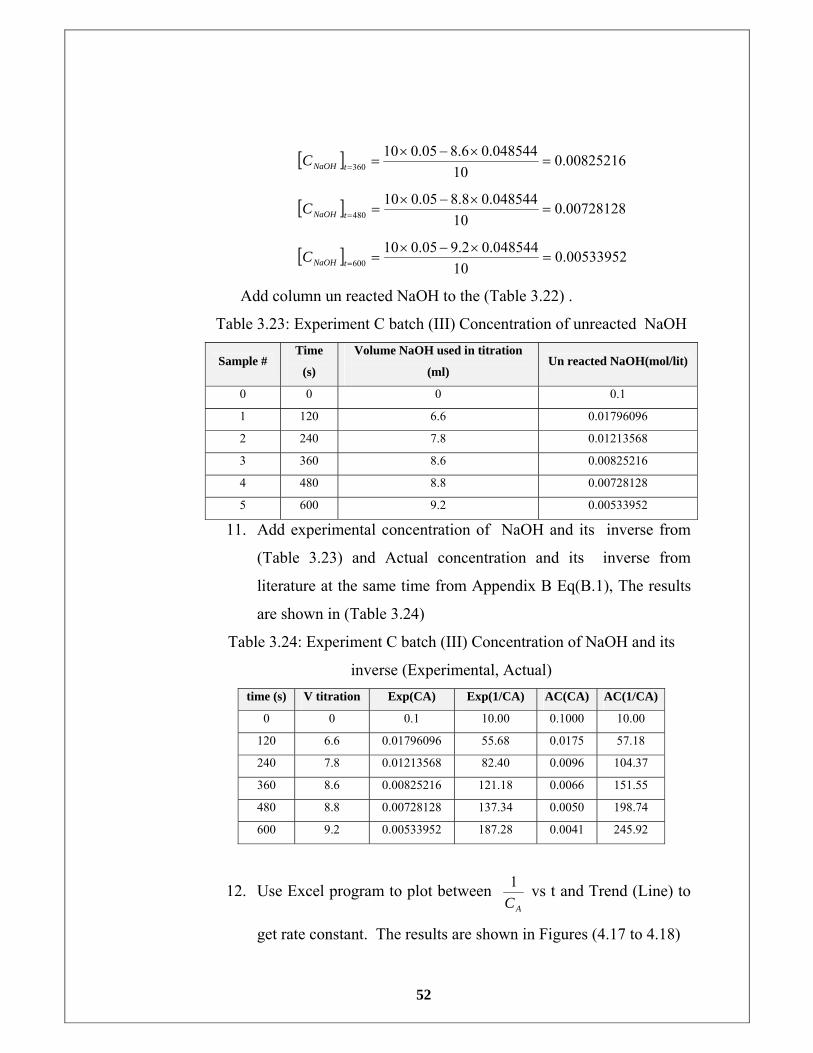
52
[ ] 0.0082521610
048544.06.805.010360 =
×−×==tNaOHC
[ ] 0.0072812810
048544.08.805.010480 =
×−×==tNaOHC
[ ] 0.0053395210
048544.02.905.010600 =
×−×==tNaOHC
Add column un reacted NaOH to the (Table 3.22) .
Table 3.23: Experiment C batch (III) Concentration of unreacted NaOH
Sample # Time
(s)
Volume NaOH used in titration
(ml) Un reacted NaOH(mol/lit)
0 0 0 0.1
1 120 6.6 0.01796096
2 240 7.8 0.01213568
3 360 8.6 0.00825216
4 480 8.8 0.00728128
5 600 9.2 0.00533952
11. Add experimental concentration of NaOH and its inverse from
(Table 3.23) and Actual concentration and its inverse from
literature at the same time from Appendix B Eq(B.1), The results
are shown in (Table 3.24)
Table 3.24: Experiment C batch (III) Concentration of NaOH and its
inverse (Experimental, Actual) time (s) V titration Exp(CA) Exp(1/CA) AC(CA) AC(1/CA)
0 0 0.1 10.00 0.1000 10.00
120 6.6 0.01796096 55.68 0.0175 57.18
240 7.8 0.01213568 82.40 0.0096 104.37
360 8.6 0.00825216 121.18 0.0066 151.55
480 8.8 0.00728128 137.34 0.0050 198.74
600 9.2 0.00533952 187.28 0.0041 245.92
12. Use Excel program to plot between AC
1 vs t and Trend (Line) to
get rate constant. The results are shown in Figures (4.17 to 4.18)
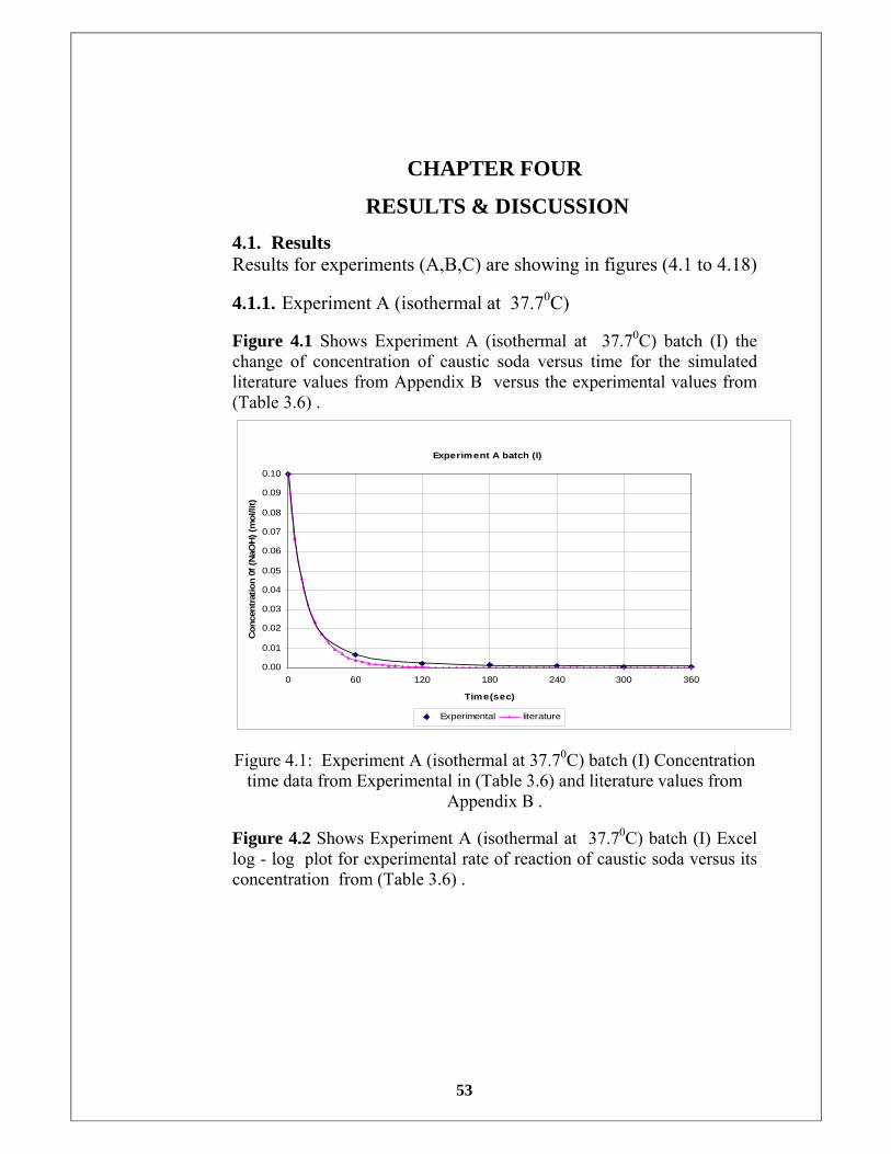
53
CHAPTER FOUR
RESULTS & DISCUSSION 4.1. Results Results for experiments (A,B,C) are showing in figures (4.1 to 4.18)
4.1.1. Experiment A (isothermal at 37.70C)
Figure 4.1 Shows Experiment A (isothermal at 37.70C) batch (I) the change of concentration of caustic soda versus time for the simulated literature values from Appendix B versus the experimental values from (Table 3.6) .
Experiment A batch (I)
0.00
0.01
0.02
0.03
0.04
0.05
0.06
0.07
0.08
0.09
0.10
0 60 120 180 240 300 360
Time(sec)
Con
cent
ratio
n 0f
(NaO
H) (
mol
/lit)
Experimental literature
Figure 4.1: Experiment A (isothermal at 37.70C) batch (I) Concentration time data from Experimental in (Table 3.6) and literature values from
Appendix B .
Figure 4.2 Shows Experiment A (isothermal at 37.70C) batch (I) Excel log - log plot for experimental rate of reaction of caustic soda versus its concentration from (Table 3.6) .
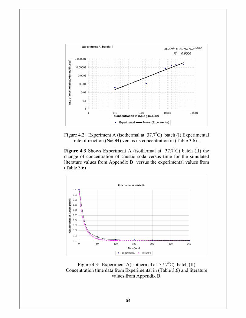
54
Experiment A batch (I)-dCA/dt = 0.0751*CA1.2283
R2 = 0.9006
0.000001
0.00001
0.0001
0.001
0.01
0.1
10.00010.0010.010.11
Concentration 0f (NaOH) (mol/lit)
rate
of r
eact
ion
(NaO
H) (
mol
/lit.s
ec)
Experimental Pow er (Experimental)
Figure 4.2: Experiment A (isothermal at 37.70C) batch (I) Experimental rate of reaction (NaOH) versus its concentration in (Table 3.6) .
Figure 4.3 Shows Experiment A (isothermal at 37.70C) batch (II) the change of concentration of caustic soda versus time for the simulated literature values from Appendix B versus the experimental values from (Table 3.6) .
Experiment A batch (II)
0.00
0.01
0.02
0.03
0.04
0.05
0.06
0.07
0.08
0.09
0.10
0 60 120 180 240 300 360
Time(sec)
Con
cent
ratio
n 0f
(NaO
H) (
mol
/lit)
Experimental literaturel
Figure 4.3: Experiment A(isothermal at 37.70C) batch (II) Concentration time data from Experimental in (Table 3.6) and literature
values from Appendix B.
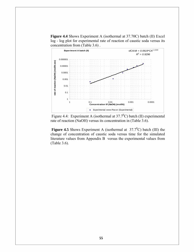
55
Figure 4.4 Shows Experiment A (isothermal at 37.70C) batch (II) Excel log - log plot for experimental rate of reaction of caustic soda versus its concentration from (Table 3.6) .
Experiment A batch (II) -dCA/dt = 0.0619*CA1.1316
R2 = 0.9296
0.000001
0.00001
0.0001
0.001
0.01
0.1
10.00010.0010.010.11
Concentration 0f (NaOH) (mol/lit)
rate
of r
eact
ion
(NaO
H) (
mol
/lit.s
ec)
Experimental Pow er (Experimental)
Figure 4.4: Experiment A (isothermal at 37.70C) batch (II) experimental rate of reaction (NaOH) versus its concentration in (Table 3.6). Figure 4.5 Shows Experiment A (isothermal at 37.70C) batch (III) the change of concentration of caustic soda versus time for the simulated literature values from Appendix B versus the experimental values from (Table 3.6).
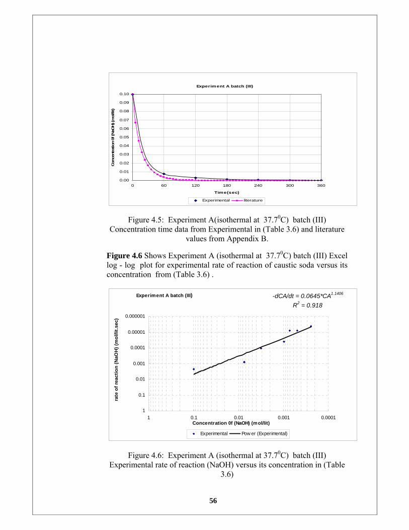
56
Experiment A batch (III)
0.00
0.01
0.02
0.03
0.04
0.05
0.06
0.07
0.08
0.09
0.10
0 60 120 180 240 300 360
Time(sec)
Con
cent
ratio
n 0f
(NaO
H) (
mol
/lit)
Experimental literature
Figure 4.5: Experiment A(isothermal at 37.70C) batch (III) Concentration time data from Experimental in (Table 3.6) and literature
values from Appendix B.
Figure 4.6 Shows Experiment A (isothermal at 37.70C) batch (III) Excel log - log plot for experimental rate of reaction of caustic soda versus its concentration from (Table 3.6) .
Experiment A batch (III) -dCA/dt = 0.0645*CA1.1406
R2 = 0.918
0.000001
0.00001
0.0001
0.001
0.01
0.1
10.00010.0010.010.11
Concentration 0f (NaOH) (mol/lit)
rate
of r
eact
ion
(NaO
H) (
mol
/lit.s
ec)
Experimental Pow er (Experimental)
Figure 4.6: Experiment A (isothermal at 37.70C) batch (III) Experimental rate of reaction (NaOH) versus its concentration in (Table
3.6)
57
4.1.2. Experiment B (isothermal at 37.70C)
Figure 4.7 Shows Experiment B (isothermal at 37.70C) batch (I) the change of concentration of caustic soda versus time for the simulated literature values from Appendix B versus the experimental values from (Table 3.12).
Experiment B batch (I)
0
0.01
0.02
0.03
0.04
0.05
0.06
0.07
0.08
0.09
0.1
0 120 240 360 480 600 720
Time(sec)
Con
cent
ratio
n 0f
(NaO
H) (
mol
/lit)
Experimental literature
Figure 4.7: Experiment B (isothermal at 37.70C) batch (I) Concentration time data from Experimental in (Table 3.12) and literature values from
Appendix B.
Figure 4.8 Shows Experiment B (isothermal at 37.70C) batch (I) Excel log - log plot for experimental rate of reaction of caustic soda versus its concentration from (Table 3.12).
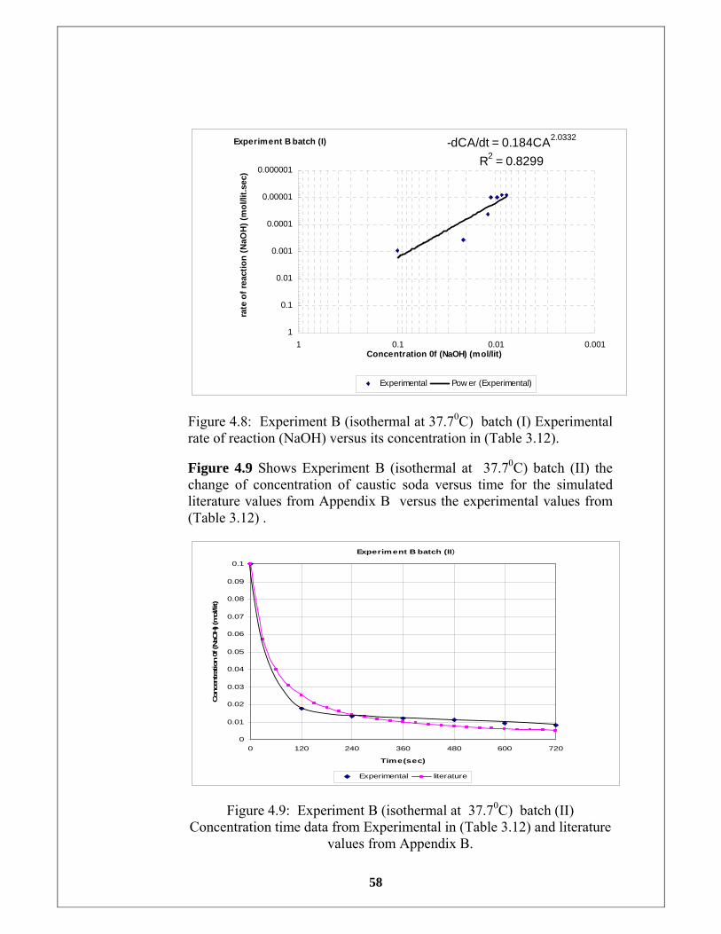
58
Experiment B batch (I) -dCA/dt = 0.184CA2.0332
R2 = 0.82990.000001
0.00001
0.0001
0.001
0.01
0.1
10.0010.010.11
Concentration 0f (NaOH) (mol/lit)
rate
of r
eact
ion
(NaO
H) (
mol
/lit.s
ec)
Experimental Pow er (Experimental)
Figure 4.8: Experiment B (isothermal at 37.70C) batch (I) Experimental rate of reaction (NaOH) versus its concentration in (Table 3.12).
Figure 4.9 Shows Experiment B (isothermal at 37.70C) batch (II) the change of concentration of caustic soda versus time for the simulated literature values from Appendix B versus the experimental values from (Table 3.12) .
Experiment B batch (II)
0
0.01
0.02
0.03
0.04
0.05
0.06
0.07
0.08
0.09
0.1
0 120 240 360 480 600 720
Time(sec)
Con
cent
ratio
n 0f
(NaO
H) (
mol
/lit)
Experimental literature
Figure 4.9: Experiment B (isothermal at 37.70C) batch (II) Concentration time data from Experimental in (Table 3.12) and literature
values from Appendix B.
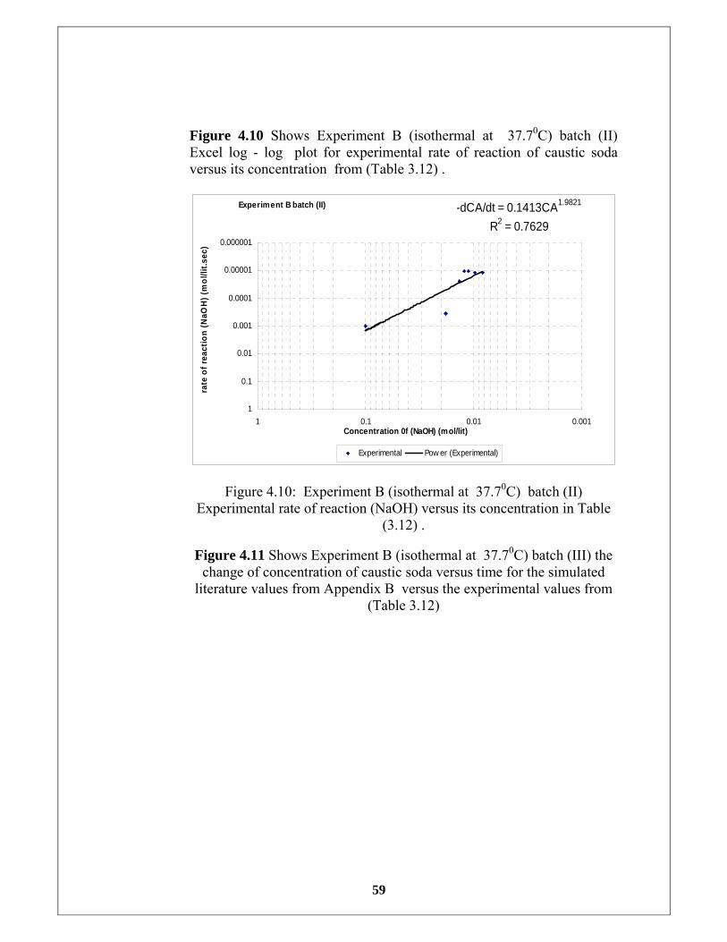
59
Figure 4.10 Shows Experiment B (isothermal at 37.70C) batch (II) Excel log - log plot for experimental rate of reaction of caustic soda versus its concentration from (Table 3.12) .
Experiment B batch (II) -dCA/dt = 0.1413CA1.9821
R2 = 0.76290.000001
0.00001
0.0001
0.001
0.01
0.1
10.0010.010.11
Concentration 0f (NaOH) (mol/lit)
rate
of r
eact
ion
(NaO
H) (
mol
/lit.s
ec)
Experimental Pow er (Experimental)
Figure 4.10: Experiment B (isothermal at 37.70C) batch (II) Experimental rate of reaction (NaOH) versus its concentration in Table
(3.12) .
Figure 4.11 Shows Experiment B (isothermal at 37.70C) batch (III) the change of concentration of caustic soda versus time for the simulated
literature values from Appendix B versus the experimental values from (Table 3.12)
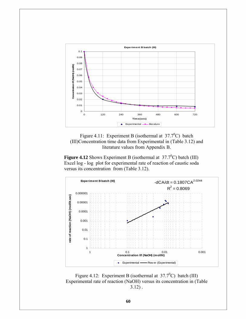
60
Experiment B batch (III)
0
0.01
0.02
0.03
0.04
0.05
0.06
0.07
0.08
0.09
0.1
0 120 240 360 480 600 720
Time(sec)
Con
cent
ratio
n 0f
(NaO
H) (
mol
/lit)
Experimental literature
Figure 4.11: Experiment B (isothermal at 37.70C) batch (III)Concentration time data from Experimental in (Table 3.12) and
literature values from Appendix B.
Figure 4.12 Shows Experiment B (isothermal at 37.70C) batch (III) Excel log - log plot for experimental rate of reaction of caustic soda versus its concentration from (Table 3.12).
Experiment B batch (III) -dCA/dt = 0.1807CA2.0244
R2 = 0.80690.000001
0.00001
0.0001
0.001
0.01
0.1
10.0010.010.11
Concentration 0f (NaOH) (mol/lit)
rate
of r
eact
ion
(NaO
H) (
mol
/lit.s
ec)
Experimental Pow er (Experimental)
Figure 4.12: Experiment B (isothermal at 37.70C) batch (III) Experimental rate of reaction (NaOH) versus its concentration in (Table
3.12) .
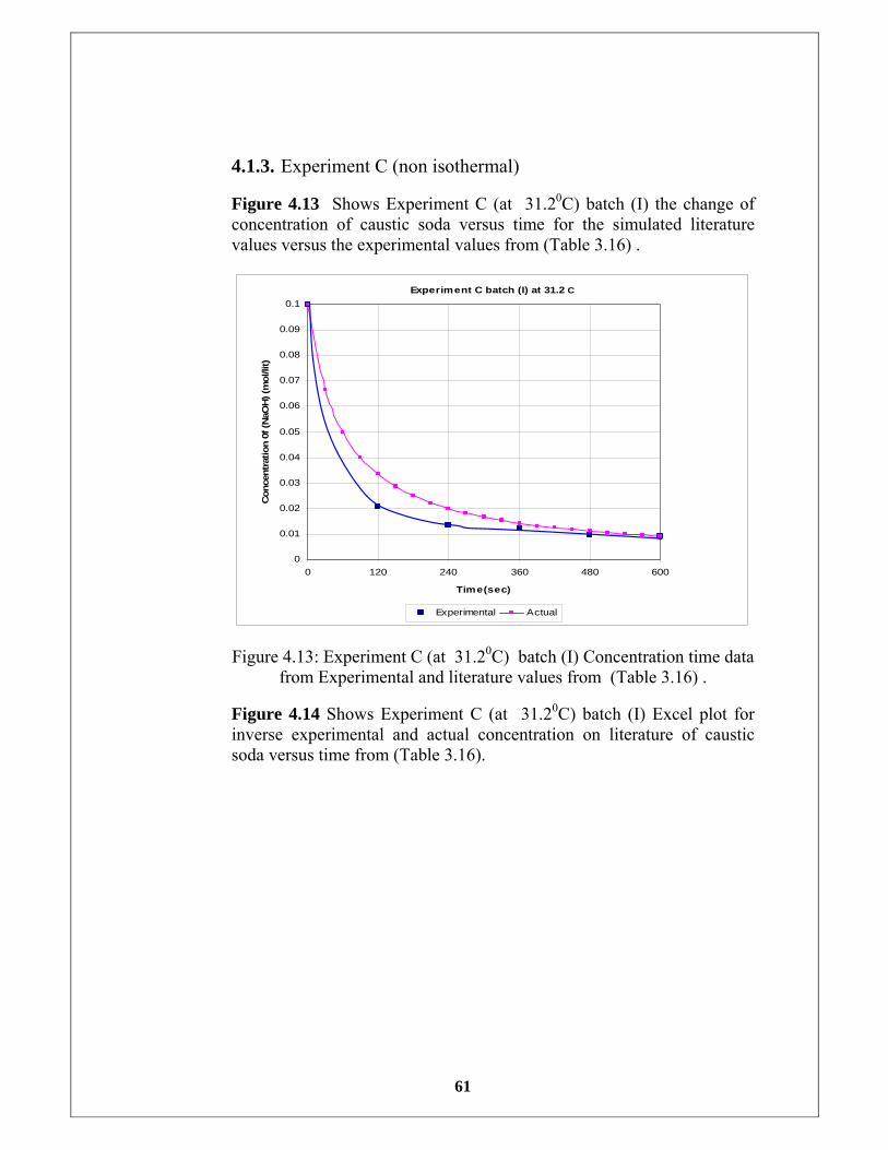
61
4.1.3. Experiment C (non isothermal)
Figure 4.13 Shows Experiment C (at 31.20C) batch (I) the change of concentration of caustic soda versus time for the simulated literature values versus the experimental values from (Table 3.16) .
Experiment C batch (I) at 31.2 C
0
0.01
0.02
0.03
0.04
0.05
0.06
0.07
0.08
0.09
0.1
0 120 240 360 480 600
Time(sec)
Con
cent
ratio
n 0f
(NaO
H) (
mol
/lit)
Experimental Actual
Figure 4.13: Experiment C (at 31.20C) batch (I) Concentration time data from Experimental and literature values from (Table 3.16) .
Figure 4.14 Shows Experiment C (at 31.20C) batch (I) Excel plot for inverse experimental and actual concentration on literature of caustic soda versus time from (Table 3.16).
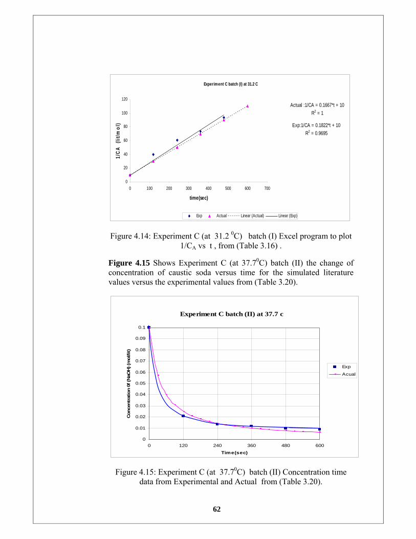
62
Experiment C batch (I) at 31.2 C
Actual :1/CA = 0.1667*t + 10R2 = 1
Exp:1/CA = 0.1822*t + 10R2 = 0.9695
0
20
40
60
80
100
120
0 100 200 300 400 500 600 700
time(sec)
1/C
A (l
it/m
ol)
Exp Actual Linear (Actual) Linear (Exp)
Figure 4.14: Experiment C (at 31.2 0C) batch (I) Excel program to plot 1/CA vs t , from (Table 3.16) .
Figure 4.15 Shows Experiment C (at 37.70C) batch (II) the change of concentration of caustic soda versus time for the simulated literature values versus the experimental values from (Table 3.20).
Experiment C batch (II) at 37.7 c
0
0.01
0.02
0.03
0.04
0.05
0.06
0.07
0.08
0.09
0.1
0 120 240 360 480 600Time(sec)
Con
cent
ratio
n 0f
(NaO
H) (
mol
/lit)
Exp
Acual
Figure 4.15: Experiment C (at 37.70C) batch (II) Concentration time data from Experimental and Actual from (Table 3.20).
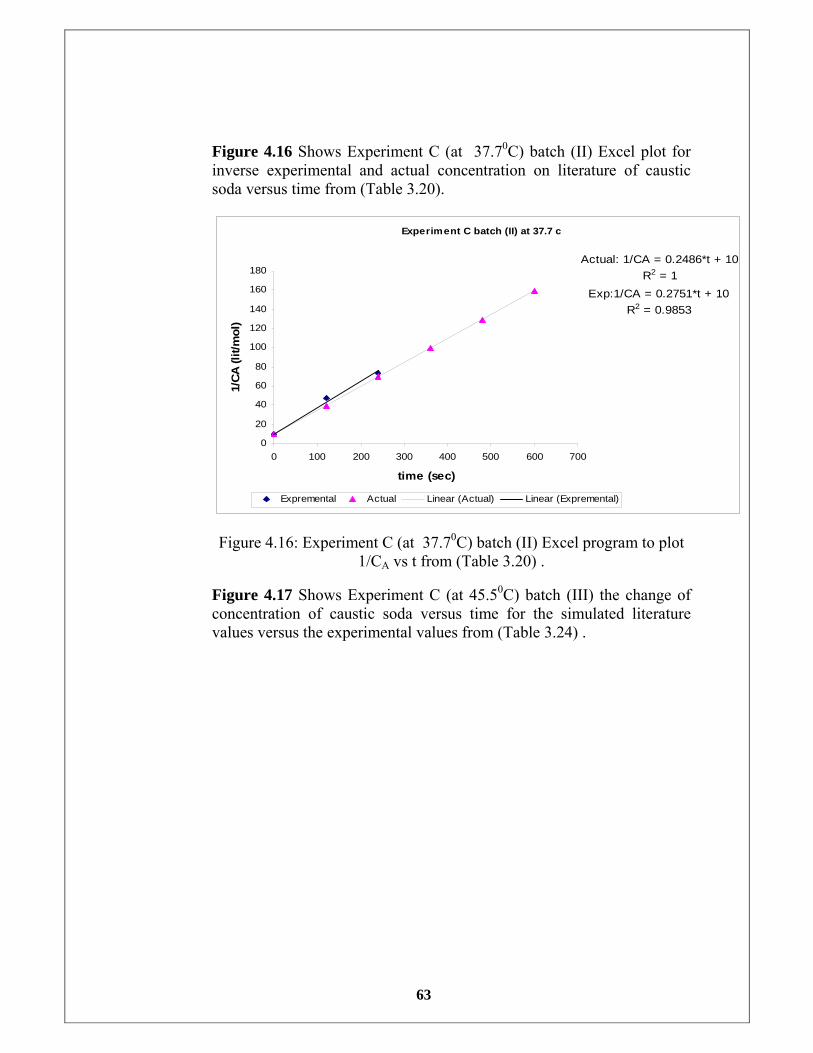
63
Figure 4.16 Shows Experiment C (at 37.70C) batch (II) Excel plot for inverse experimental and actual concentration on literature of caustic soda versus time from (Table 3.20).
Experiment C batch (II) at 37.7 c
Actual: 1/CA = 0.2486*t + 10R2 = 1
Exp:1/CA = 0.2751*t + 10R2 = 0.9853
0
20
40
60
80
100
120
140
160
180
0 100 200 300 400 500 600 700
time (sec)
1/CA
(lit/
mol
)
Expremental Actual Linear (Actual) Linear (Expremental)
Figure 4.16: Experiment C (at 37.70C) batch (II) Excel program to plot 1/CA vs t from (Table 3.20) .
Figure 4.17 Shows Experiment C (at 45.50C) batch (III) the change of concentration of caustic soda versus time for the simulated literature values versus the experimental values from (Table 3.24) .
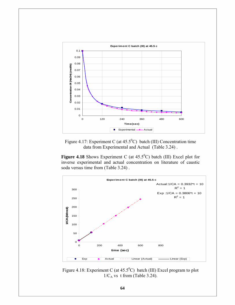
64
Experiment C batch (III) at 45.5 c
0
0.01
0.02
0.03
0.04
0.05
0.06
0.07
0.08
0.09
0.1
0 120 240 360 480 600
Time(sec)
Con
cent
ratio
n 0f
(NaO
H) (
mol
/lit)
Experimental Actual
Figure 4.17: Experiment C (at 45.50C) batch (III) Concentration time data from Experimental and Actual (Table 3.24) .
Figure 4.18 Shows Experiment C (at 45.50C) batch (III) Excel plot for inverse experimental and actual concentration on literature of caustic soda versus time from (Table 3.24) .
Experiment C batch (III) at 45.5 c
Actual:1/CA = 0.3932*t + 10R2 = 1
Exp :1/CA = 0.3806*t + 10R2 = 1
0
50
100
150
200
250
300
0 200 400 600 800
time (sec)
1/CA
(lit/
mol
)
Exp Actual Linear (Actual) Linear (Exp)
Figure 4.18: Experiment C (at 45.50C) batch (III) Excel program to plot 1/CA vs t from (Table 3.24).
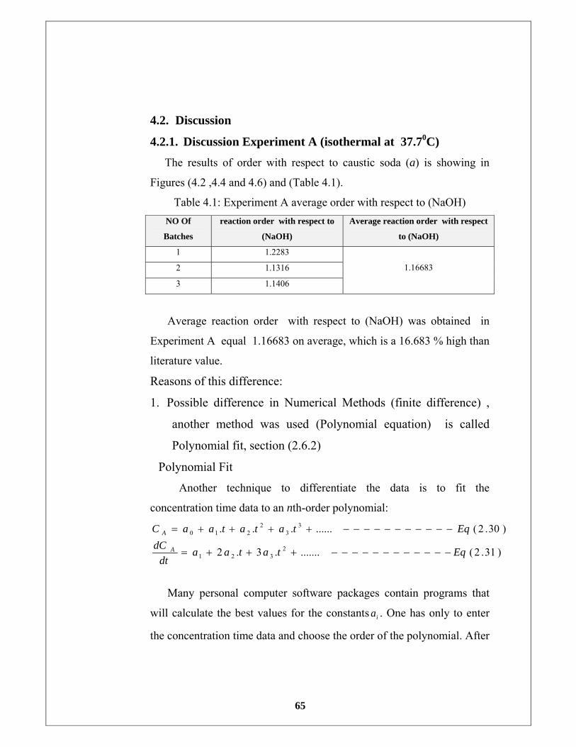
65
4.2. Discussion
4.2.1. Discussion Experiment A (isothermal at 37.70C)
The results of order with respect to caustic soda (a) is showing in
Figures (4.2 ,4.4 and 4.6) and (Table 4.1).
Table 4.1: Experiment A average order with respect to (NaOH) NO Of
Batches
reaction order with respect to
(NaOH)
Average reaction order with respect
to (NaOH)
1 1.2283
2 1.1316
3 1.1406
1.16683
Average reaction order with respect to (NaOH) was obtained in
Experiment A equal 1.16683 on average, which is a 16.683 % high than
literature value.
Reasons of this difference:
1. Possible difference in Numerical Methods (finite difference) ,
another method was used (Polynomial equation) is called
Polynomial fit, section (2.6.2)
Polynomial Fit
Another technique to differentiate the data is to fit the
concentration time data to an nth-order polynomial:
)31.2(........3.2
)30.2(.........
2321
33
2210
Eqtataadt
dCEqtatataaC
A
A
−−−−−−−−−−−−+++=
−−−−−−−−−−−++++=
Many personal computer software packages contain programs that
will calculate the best values for the constants ia . One has only to enter
the concentration time data and choose the order of the polynomial. After
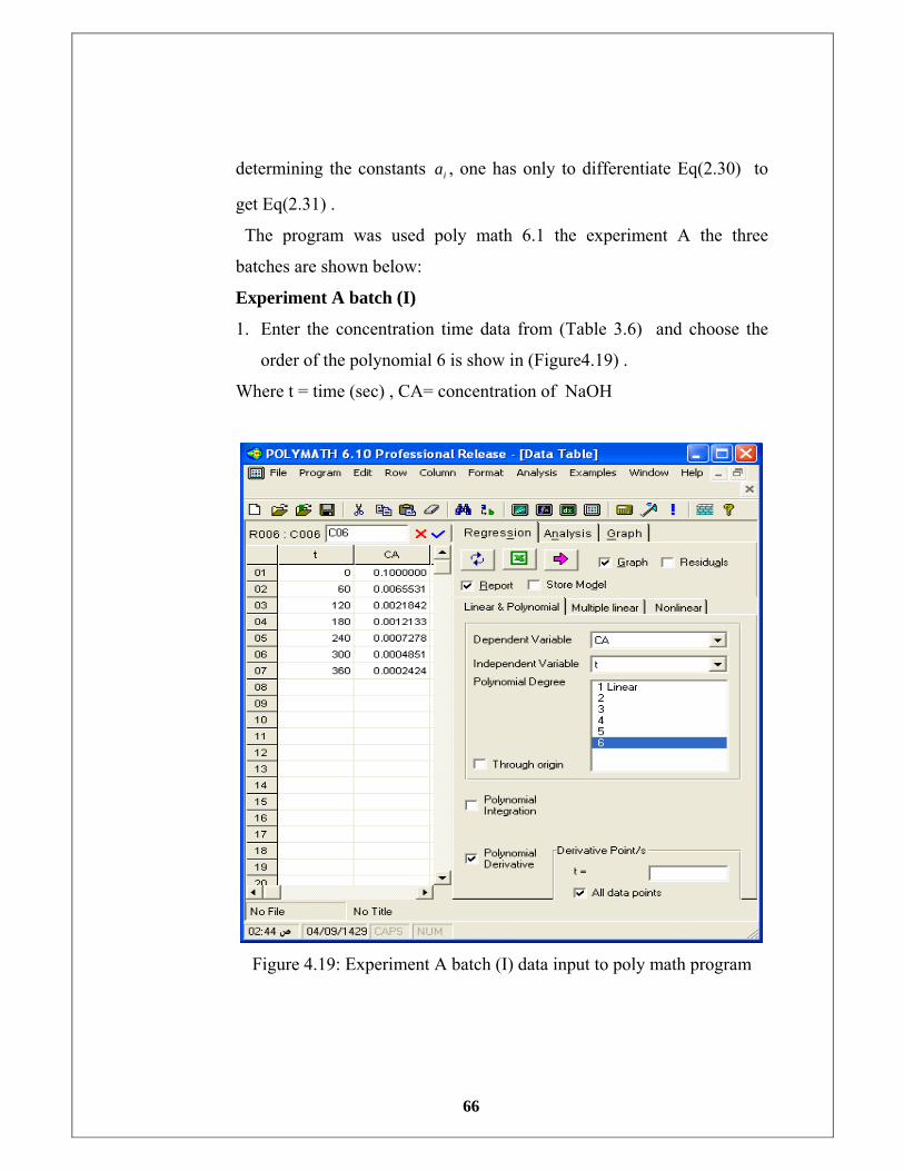
66
determining the constants ia , one has only to differentiate Eq(2.30) to
get Eq(2.31) .
The program was used poly math 6.1 the experiment A the three
batches are shown below:
Experiment A batch (I)
1. Enter the concentration time data from (Table 3.6) and choose the
order of the polynomial 6 is show in (Figure4.19) .
Where t = time (sec) , CA= concentration of NaOH
Figure 4.19: Experiment A batch (I) data input to poly math program
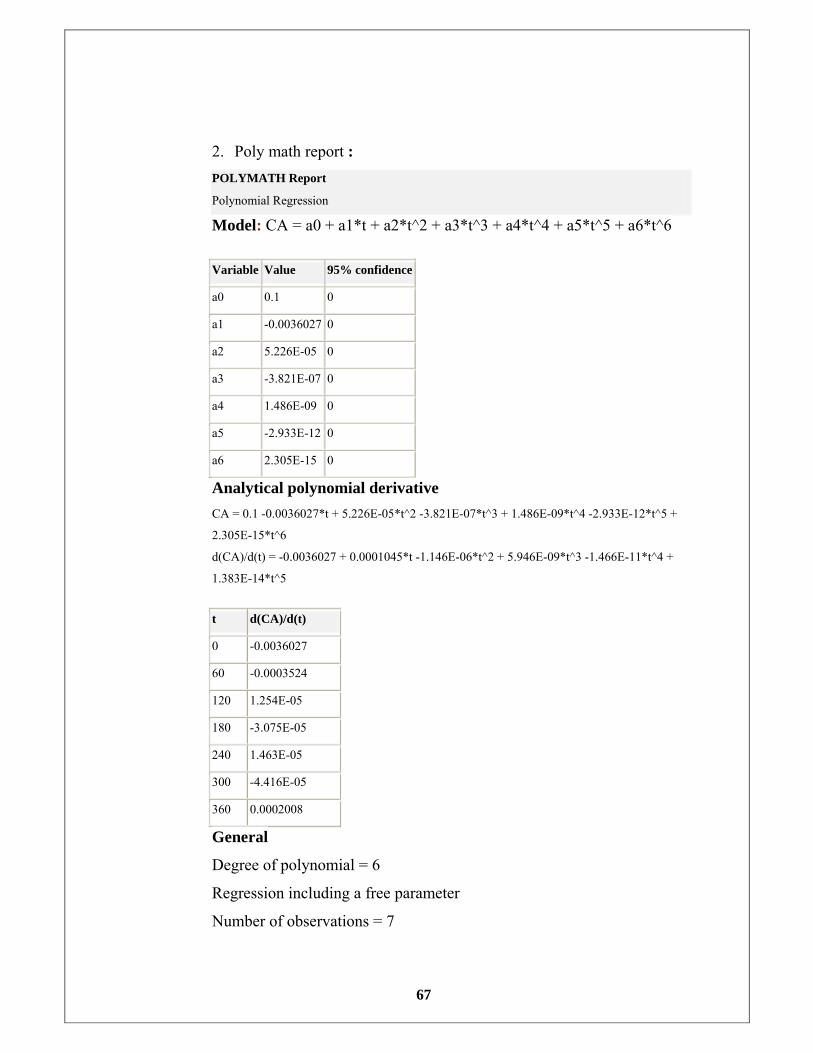
67
2. Poly math report : POLYMATH Report
Polynomial Regression
Model: CA = a0 + a1*t + a2*t^2 + a3*t^3 + a4*t^4 + a5*t^5 + a6*t^6
Variable Value 95% confidence
a0 0.1 0
a1 -0.0036027 0
a2 5.226E-05 0
a3 -3.821E-07 0
a4 1.486E-09 0
a5 -2.933E-12 0
a6 2.305E-15 0
Analytical polynomial derivative CA = 0.1 -0.0036027*t + 5.226E-05*t^2 -3.821E-07*t^3 + 1.486E-09*t^4 -2.933E-12*t^5 +
2.305E-15*t^6
d(CA)/d(t) = -0.0036027 + 0.0001045*t -1.146E-06*t^2 + 5.946E-09*t^3 -1.466E-11*t^4 +
1.383E-14*t^5
t d(CA)/d(t)
0 -0.0036027
60 -0.0003524
120 1.254E-05
180 -3.075E-05
240 1.463E-05
300 -4.416E-05
360 0.0002008
General
Degree of polynomial = 6
Regression including a free parameter
Number of observations = 7

68
Statistics
R^2 1.
R^2adj 0
Rmsd 3.412E-12
Variance 1.0E+99
Source data points and calculated data points
t CA CA calc Delta CA
1 0 0.1 0.1 9.43E-13
2 60 0.0065531 0.0065531 -5.299E-12
3 120 0.0021842 0.0021842 1.257E-11
4 180 0.0012133 0.0012133 -1.548E-11
5 240 0.0007278 0.0007278 1.12E-11
6 300 0.0004851 0.0004851 -4.284E-12
7 360 0.0002424 0.0002424 -4.187E-13
Graph
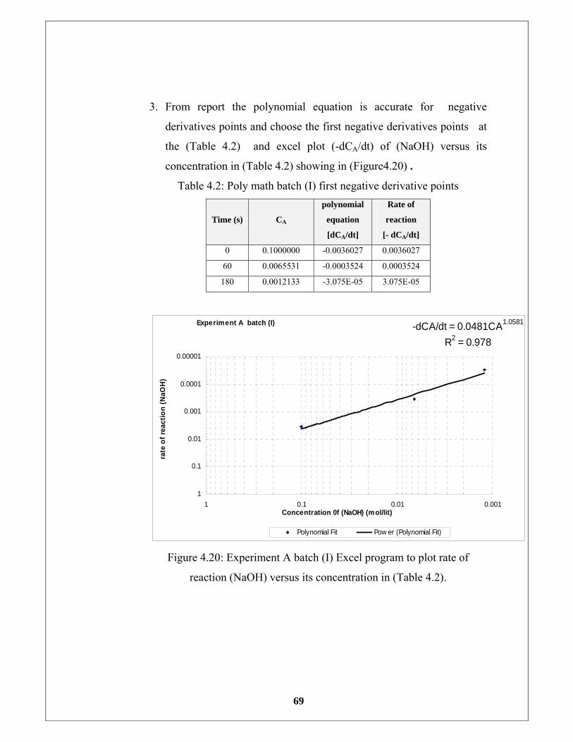
69
3. From report the polynomial equation is accurate for negative
derivatives points and choose the first negative derivatives points at
the (Table 4.2) and excel plot (-dCA/dt) of (NaOH) versus its
concentration in (Table 4.2) showing in (Figure4.20) .
Table 4.2: Poly math batch (I) first negative derivative points
Time (s) CA
polynomial
equation
[dCA/dt]
Rate of
reaction
[- dCA/dt]
0 0.1000000 -0.0036027 0.0036027
60 0.0065531 -0.0003524 0.0003524
180 0.0012133 -3.075E-05 3.075E-05
Experiment A batch (I) -dCA/dt = 0.0481CA1.0581
R2 = 0.9780.00001
0.0001
0.001
0.01
0.1
10.0010.010.11
Concentration 0f (NaOH) (mol/lit)
rate
of r
eact
ion
(NaO
H)
Polynomial Fit Pow er (Polynomial Fit)
Figure 4.20: Experiment A batch (I) Excel program to plot rate of
reaction (NaOH) versus its concentration in (Table 4.2).
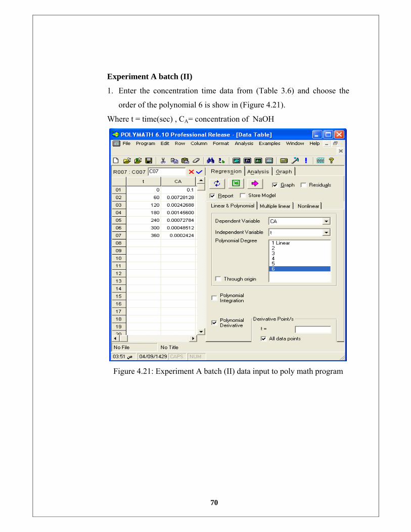
70
Experiment A batch (II)
1. Enter the concentration time data from (Table 3.6) and choose the
order of the polynomial 6 is show in (Figure 4.21).
Where t = time(sec) , CA= concentration of NaOH
Figure 4.21: Experiment A batch (II) data input to poly math program
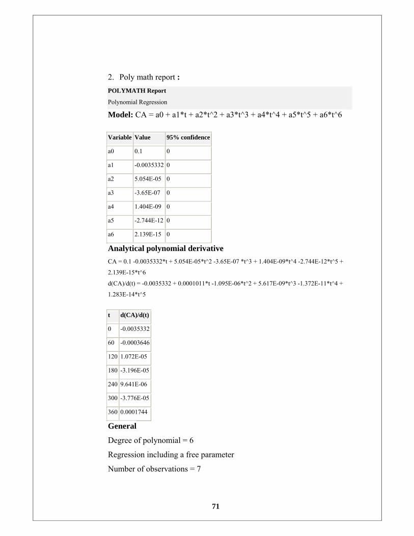
71
2. Poly math report : POLYMATH Report
Polynomial Regression
Model: CA = a0 + a1*t + a2*t^2 + a3*t^3 + a4*t^4 + a5*t^5 + a6*t^6
Variable Value 95% confidence
a0 0.1 0
a1 -0.0035332 0
a2 5.054E-05 0
a3 -3.65E-07 0
a4 1.404E-09 0
a5 -2.744E-12 0
a6 2.139E-15 0
Analytical polynomial derivative CA = 0.1 -0.0035332*t + 5.054E-05*t^2 -3.65E-07 *t^3 + 1.404E-09*t^4 -2.744E-12*t^5 +
2.139E-15*t^6
d(CA)/d(t) = -0.0035332 + 0.0001011*t -1.095E-06*t^2 + 5.617E-09*t^3 -1.372E-11*t^4 +
1.283E-14*t^5
t d(CA)/d(t)
0 -0.0035332
60 -0.0003646
120 1.072E-05
180 -3.196E-05
240 9.641E-06
300 -3.776E-05
360 0.0001744
General
Degree of polynomial = 6
Regression including a free parameter
Number of observations = 7
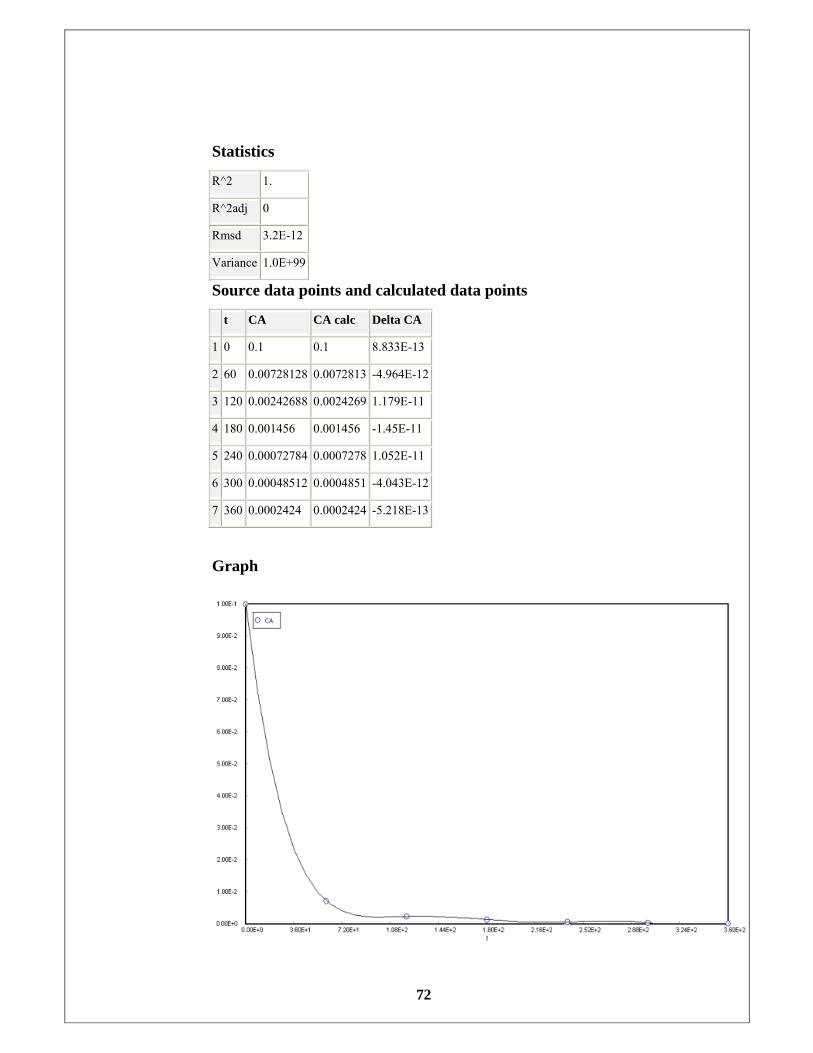
72
Statistics
R^2 1.
R^2adj 0
Rmsd 3.2E-12
Variance 1.0E+99
Source data points and calculated data points
t CA CA calc Delta CA
1 0 0.1 0.1 8.833E-13
2 60 0.00728128 0.0072813 -4.964E-12
3 120 0.00242688 0.0024269 1.179E-11
4 180 0.001456 0.001456 -1.45E-11
5 240 0.00072784 0.0007278 1.052E-11
6 300 0.00048512 0.0004851 -4.043E-12
7 360 0.0002424 0.0002424 -5.218E-13
Graph
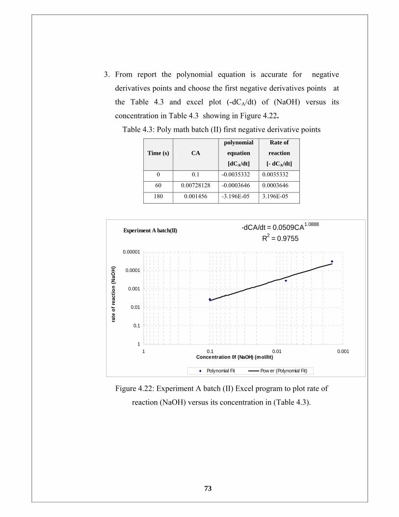
73
3. From report the polynomial equation is accurate for negative
derivatives points and choose the first negative derivatives points at
the Table 4.3 and excel plot (-dCA/dt) of (NaOH) versus its
concentration in Table 4.3 showing in Figure 4.22.
Table 4.3: Poly math batch (II) first negative derivative points
Time (s) CA
polynomial
equation
[dCA/dt]
Rate of
reaction
[- dCA/dt]
0 0.1 -0.0035332 0.0035332
60 0.00728128 -0.0003646 0.0003646
180 0.001456 -3.196E-05 3.196E-05
Experiment A batch(II) -dCA/dt = 0.0509CA1.0888
R2 = 0.9755
0.00001
0.0001
0.001
0.01
0.1
10.0010.010.11
Concentration 0f (NaOH) (mol/lit)
rate
of r
eact
ion
(NaO
H)
Polynomial Fit Pow er (Polynomial Fit)
Figure 4.22: Experiment A batch (II) Excel program to plot rate of
reaction (NaOH) versus its concentration in (Table 4.3).
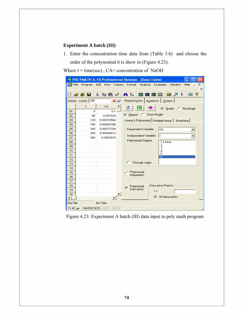
74
Experiment A batch (III)
1. Enter the concentration time data from (Table 3.6) and choose the
order of the polynomial 6 is show in (Figure 4.23).
Where t = time(sec) , CA= concentration of NaOH
Figure 4.23: Experiment A batch (III) data input to poly math program

75
2. Poly math report : POLYMATH Report
Polynomial Regression
Model: CA = a0 + a1*t + a2*t^2 + a3*t^3 + a4*t^4 + a5*t^5 + a6*t^6
Variable Value 95% confidence
a0 0.1 0
a1 -0.0036539 0
a2 5.481E-05 0
a3 -4.151E-07 0
a4 1.666E-09 0
a5 -3.375E-12 0
a6 2.71E-15 0
Analytical polynomial derivative CA = 0.1 -0.0036539*t + 5.481E-05*t^2 -4.151E-07*t^3 + 1.666E-09*t^4 -3.375E-12*t^5 +
2.71E-15 *t^6
d(CA)/d(t) = -0.0036539 + 0.0001096*t -1.245E-06*t^2 + 6.666E-09*t^3 -1.688E-11*t^4 +
1.626E-14*t^5
t d(CA)/d(t)
0 -0.0036539
60 -0.000326
120 8.765E-06
180 -4.045E-05
240 2.596E-05
300 -6.034E-05
360 0.000269
General
Degree of polynomial = 6
Regression including a free parameter
Number of observations = 7
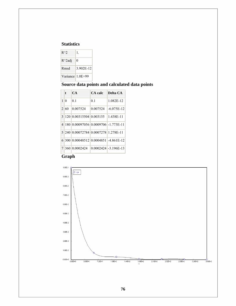
76
Statistics
R^2 1.
R^2adj 0
Rmsd 3.902E-12
Variance 1.0E+99
Source data points and calculated data points
t CA CA calc Delta CA
1 0 0.1 0.1 1.082E-12
2 60 0.007524 0.007524 -6.075E-12
3 120 0.00315504 0.003155 1.438E-11
4 180 0.00097056 0.0009706 -1.773E-11
5 240 0.00072784 0.0007278 1.278E-11
6 300 0.00048512 0.0004851 -4.861E-12
7 360 0.0002424 0.0002424 -3.196E-13
Graph
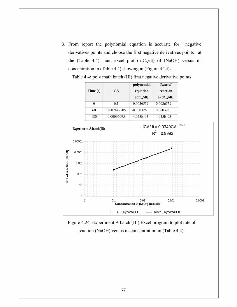
77
3. From report the polynomial equation is accurate for negative
derivatives points and choose the first negative derivatives points at
the (Table 4.4) and excel plot (-dCA/dt) of (NaOH) versus its
concentration in (Table 4.4) showing in (Figure 4.24).
Table 4.4: poly math batch (III) first negative derivative points
Time (s) CA
polynomial
equation
[dCA/dt]
Rate of
reaction
[- dCA/dt]
0 0.1 -0.0036539 0.0036539
60 0.007449505 -0.000326 0.000326
180 0.00096095 -4.045E-05 4.045E-05
Experiment A batch(III) -dCA/dt = 0.0349CA0.9678
R2 = 0.9993
0.00001
0.0001
0.001
0.01
0.1
10.00010.0010.010.11
Concentration 0f (NaOH) (mol/lit)
rate
of r
eact
ion
(NaO
H)
Polynomial Fit Pow er (Polynomial Fit)
Figure 4.24: Experiment A batch (III) Excel program to plot rate of
reaction (NaOH) versus its concentration in (Table 4.4).
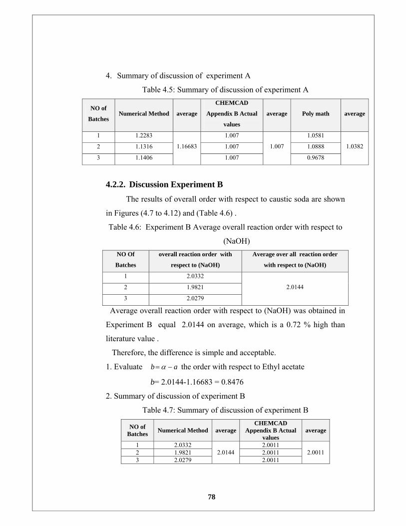
78
4. Summary of discussion of experiment A
Table 4.5: Summary of discussion of experiment A
NO of
Batches Numerical Method average
CHEMCAD
Appendix B Actual
values
average Poly math average
1 1.2283 1.007 1.0581
2 1.1316 1.007 1.0888
3 1.1406
1.16683
1.007
1.007
0.9678
1.0382
4.2.2. Discussion Experiment B
The results of overall order with respect to caustic soda are shown
in Figures (4.7 to 4.12) and (Table 4.6) .
Table 4.6: Experiment B Average overall reaction order with respect to
(NaOH) NO Of
Batches
overall reaction order with
respect to (NaOH)
Average over all reaction order
with respect to (NaOH)
1 2.0332
2 1.9821
3 2.0279
2.0144
Average overall reaction order with respect to (NaOH) was obtained in
Experiment B equal 2.0144 on average, which is a 0.72 % high than
literature value .
Therefore, the difference is simple and acceptable.
1. Evaluate ab −= α the order with respect to Ethyl acetate
b= 2.0144-1.16683 = 0.8476
2. Summary of discussion of experiment B
Table 4.7: Summary of discussion of experiment B
NO of Batches Numerical Method average
CHEMCAD Appendix B Actual
values average
1 2.0332 2.0011 2 1.9821 2.0011 3 2.0279
2.0144 2.0011
2.0011
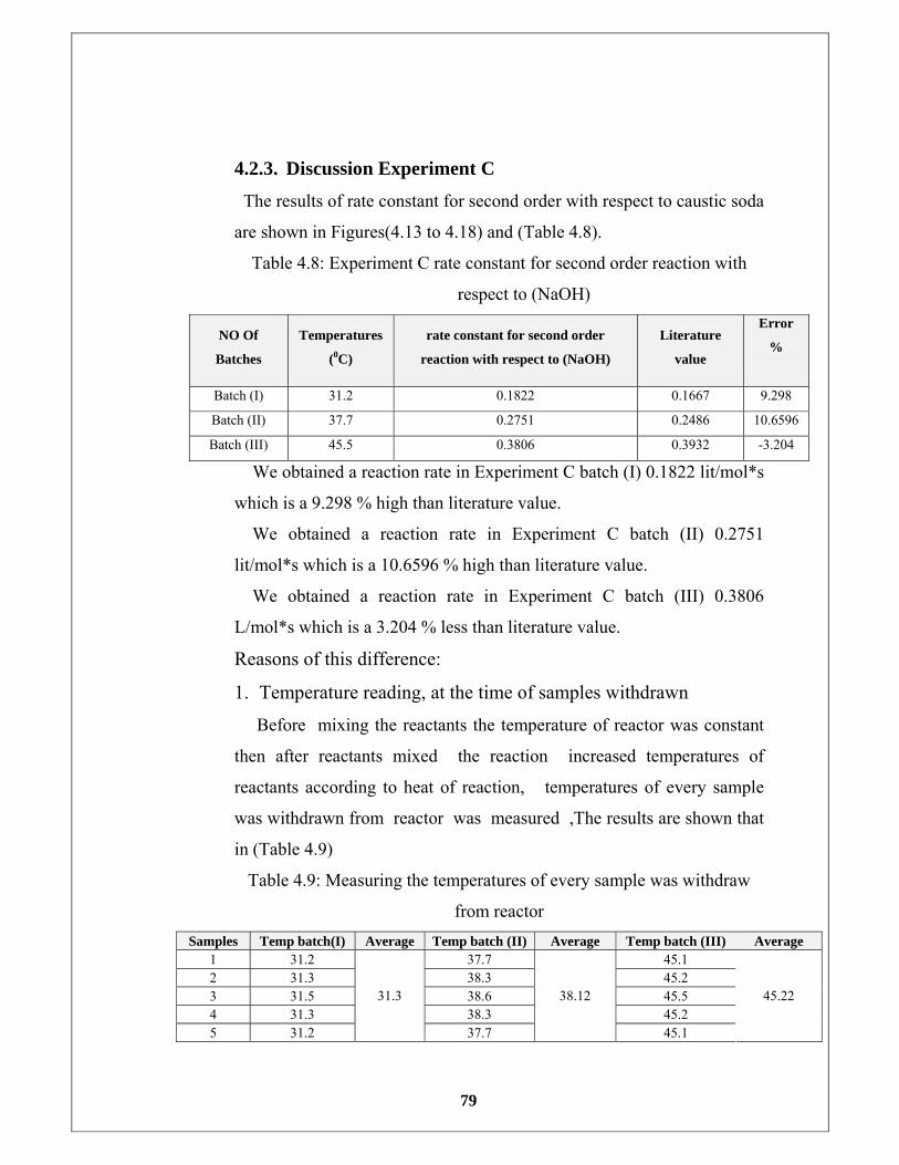
79
4.2.3. Discussion Experiment C
The results of rate constant for second order with respect to caustic soda
are shown in Figures(4.13 to 4.18) and (Table 4.8).
Table 4.8: Experiment C rate constant for second order reaction with
respect to (NaOH)
NO Of
Batches
Temperatures
(0C)
rate constant for second order
reaction with respect to (NaOH)
Literature
value
Error
%
Batch (I) 31.2 0.1822 0.1667 9.298
Batch (II) 37.7 0.2751 0.2486 10.6596
Batch (III) 45.5 0.3806 0.3932 -3.204
We obtained a reaction rate in Experiment C batch (I) 0.1822 lit/mol*s
which is a 9.298 % high than literature value.
We obtained a reaction rate in Experiment C batch (II) 0.2751
lit/mol*s which is a 10.6596 % high than literature value.
We obtained a reaction rate in Experiment C batch (III) 0.3806
L/mol*s which is a 3.204 % less than literature value.
Reasons of this difference:
1. Temperature reading, at the time of samples withdrawn
Before mixing the reactants the temperature of reactor was constant
then after reactants mixed the reaction increased temperatures of
reactants according to heat of reaction, temperatures of every sample
was withdrawn from reactor was measured ,The results are shown that
in (Table 4.9)
Table 4.9: Measuring the temperatures of every sample was withdraw
from reactor Samples Temp batch(I) Average Temp batch (II) Average Temp batch (III) Average
1 31.2 37.7 45.1 2 31.3 38.3 45.2 3 31.5 38.6 45.5 4 31.3 38.3 45.2 5 31.2
31.3
37.7
38.12
45.1
45.22
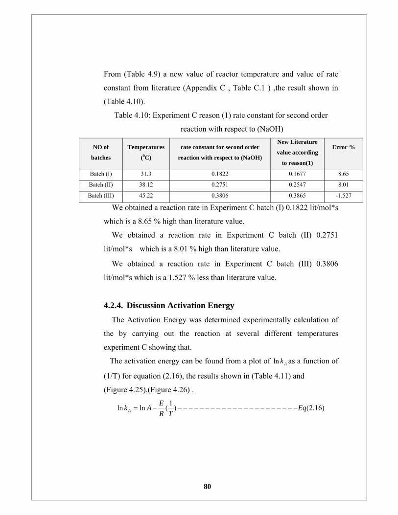
80
From (Table 4.9) a new value of reactor temperature and value of rate
constant from literature (Appendix C , Table C.1 ) ,the result shown in
(Table 4.10).
Table 4.10: Experiment C reason (1) rate constant for second order
reaction with respect to (NaOH)
NO of
batches
Temperatures
(0C)
rate constant for second order
reaction with respect to (NaOH)
New Literature
value according
to reason(1)
Error %
Batch (I) 31.3 0.1822 0.1677 8.65
Batch (II) 38.12 0.2751 0.2547 8.01
Batch (III) 45.22 0.3806 0.3865 -1.527
We obtained a reaction rate in Experiment C batch (I) 0.1822 lit/mol*s
which is a 8.65 % high than literature value.
We obtained a reaction rate in Experiment C batch (II) 0.2751
lit/mol*s which is a 8.01 % high than literature value.
We obtained a reaction rate in Experiment C batch (III) 0.3806
lit/mol*s which is a 1.527 % less than literature value.
4.2.4. Discussion Activation Energy
The Activation Energy was determined experimentally calculation of
the by carrying out the reaction at several different temperatures
experiment C showing that.
The activation energy can be found from a plot of Akln as a function of
(1/T) for equation (2.16), the results shown in (Table 4.11) and
(Figure 4.25),(Figure 4.26) .
)16.2()1(lnln EqTR
EAk A −−−−−−−−−−−−−−−−−−−−−−−=
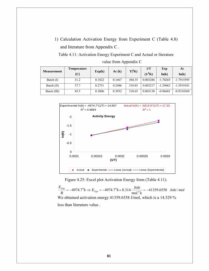
81
1) Calculation Activation Energy from Experiment C (Table 4.8)
and literature from Appendix C .
Table 4.11: Activation Energy Experiment C and Actual or literature
value from Appendix C
Measurement Temperature
[C] Exp(k) Ac (k) T(0K)
1/T
(1/0K)
Exp
ln(k)
Ac
ln(k)
Batch (I) 31.2 0.1822 0.1667 304.35 0.003286 -1.70265 -1.7915595
Batch (II) 37.7 0.2751 0.2486 310.85 0.003217 -1.29062 -1.3919101
Batch (III) 45.5 0.3806 0.3932 318.65 0.003138 -0.96601 -0.9334369
Activity Energy
Actual ln(K) = -5819.8*(1/T) + 17.33R2 = 1
Experimental ln(k) = -4974.7*(1/T) + 14.667R2 = 0.9884
-2
-1.5
-1
-0.5
00.0031 0.00315 0.0032 0.00325 0.0033
(1/T)
ln(K
)
Actual Experimental Linear (Actual) Linear (Experimental)
Figure 4.25: Excel plot Activation Energy form (Table 4.11).
molJolekmol
JolekEkR
EExp
Exp /6558.41359.
314.87.49747.4974 000 −=×−=⇒−=
We obtained activation energy 41359.6558 J/mol, which is a 14.529 %
less than literature value .
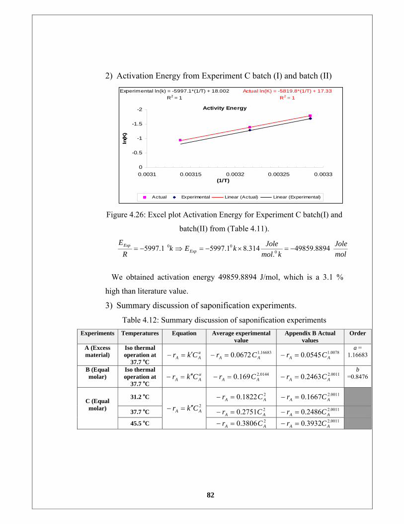
82
2) Activation Energy from Experiment C batch (I) and batch (II)
Activity Energy
Actual ln(K) = -5819.8*(1/T) + 17.33R2 = 1
Experimental ln(k) = -5997.1*(1/T) + 18.002R2 = 1
-2
-1.5
-1
-0.5
00.0031 0.00315 0.0032 0.00325 0.0033
(1/T)
ln(K
)
Actual Experimental Linear (Actual) Linear (Experimental)
Figure 4.26: Excel plot Activation Energy for Experiment C batch(I) and
batch(II) from (Table 4.11).
molJole
kmolJolekEk
RE
ExpExp 8894.49859
.314.81.59971.5997 0
00 −=×−=⇒−=
We obtained activation energy 49859.8894 J/mol, which is a 3.1 %
high than literature value.
3) Summary discussion of saponification experiments.
Table 4.12: Summary discussion of saponification experiments Experiments Temperatures Equation Average experimental
value Appendix B Actual
values Order
A (Excess material)
Iso thermal operation at
37.7 oC
aAA Ckr ′=− 16683.10672.0 AA Cr =− 0078.10545.0 AA Cr =−
a = 1.16683
B (Equal molar)
Iso thermal operation at
37.7 oC
αAA Ckr ′′=− 0144.2169.0 AA Cr =− 0011.22463.0 AA Cr =−
b =0.8476
31.2 oC 21822.0 AA Cr =− 0011.21667.0 AA Cr =−
37.7 oC 22751.0 AA Cr =− 0011.22486.0 AA Cr =− C (Equal molar)
45.5 oC
2AA Ckr ′′=−
23806.0 AA Cr =− 0011.23932.0 AA Cr =−
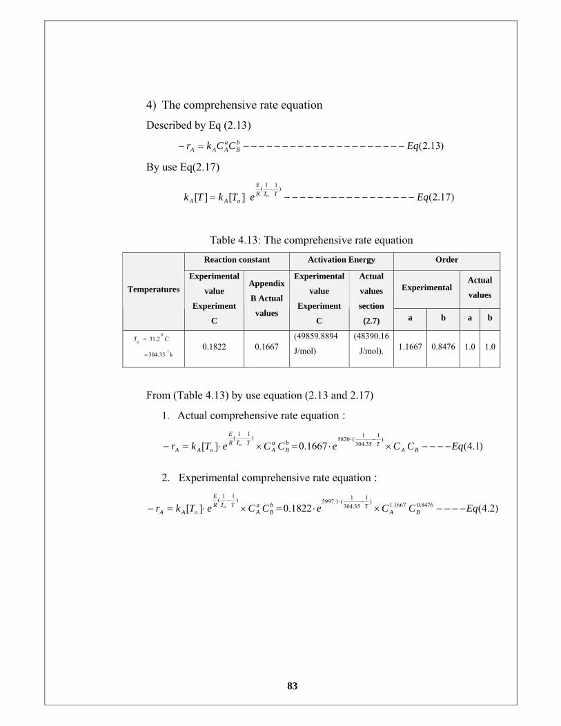
83
4) The comprehensive rate equation
Described by Eq (2.13)
)13.2(EqCCkr bB
aAAA −−−−−−−−−−−−−−−−−−−−−=−
By use Eq(2.17)
)17.2(][][)11(
EqeTkTk TTRE
oAAo −−−−−−−−−−−−−−−−−=−
Table 4.13: The comprehensive rate equation Reaction constant Activation Energy Order
Experimental Actual
values Temperatures Experimental
value
Experiment
C
Appendix
B Actual
values
Experimental
value
Experiment
C
Actual
values
section
(2.7) a b a b
k
CTo
o35.304
2.310
=
= 0.1822 0.1667 (49859.8894
J/mol)
(48390.16
J/mol). 1.1667 0.8476 1.0 1.0
From (Table 4.13) by use equation (2.13 and 2.17)
1. Actual comprehensive rate equation :
)1.4(1667.0][)1
35.3041(5820)11(
EqCCeCCeTkr BATb
BaA
TTRE
oAAo −−−−×⋅=×⋅=−
−⋅−
2. Experimental comprehensive rate equation :
)2.4(1822.0][ 8476.01667.1)135.304
1(1.5997)11(EqCCeCCeTkr BA
TbB
aA
TTRE
oAAo −−−−×⋅=×⋅=−
−⋅−
84
CHAPTER FIVE
CONCLUSION & RECOMMENDATION 5.1 Conclusion
1. The pilot - scale batch reactor has been refurbished with a minimal
cost.
2. Use of the unit with the water bath has provided better temperature
control compared with using the heater and cold water around the
jacket of reactor.
3. A saponification reaction provides a safe option for use as a case
study.
4. Reaction kinetics is in line with literature.
5. In experiment A access material (Three times the concentration) is
sufficient in this experiment. The use of the Polynomial Fit method
(poly math software) provided better than finite difference method.
6. In experiment B (equal molar) the use of finite difference method to
calculate the derivative is sufficient.
5.2 Recommendations
1. Automation for batch reactor through adding hardware and software
components such as lab view, Matlab.
2. To add experiment to fifth year undergraduate students to reinforce
their experimental skills.
85
REFERENCES 1. Fogler, S. H.; “Elements of Chemical Reaction Engineering,”
Prentice Hall, 4rd Edition (2006)
2. A. SARATH BABU,“BATCH REACTOR - Interpretation of rate
data”, (http://www.engin.umich.edu/3.Batch_reactor.ppt)
3. Tsujikawa, Hiroo, and Inoue, Hakuai. “The Reaction Rate of Alkaline
Hydrolysis of Ethyl Acetate”, Bulletin of the Chemical Society of
Japan, 39: 1837-1842
4. www.csupomona.edu/~tknguyen/che435/Notes/files_2Experiments_
Homogenuous_Batch_Reactor.pdf
5. UNIVERSITY OF MINNESOTA DULUTH - DEPARTMENT OF
CHEMICAL ENGINEERING- ChE 3211-4211,” BATCH
REACTOR “, exbatrea.pdf
86
APPENDIXES
Appendix A : Materials Safety Data Sheet (MSDS)
1. Chemical Safety Data: Sodium Hydroxide
Common
synonyms Caustic soda, soda lye
Formula NaOH
Physical
properties
Form: White semi-transparent solid, often supplied as pellets
weighing about 0.1g
Stability: Stable, but hygroscopic. Absorbs carbon dioxide
from the air.
Melting point: 318 C
Water solubility: high (dissolution is very exothermic)
Specific gravity: 2.12
Principal
hazards
Contact with the eyes can cause serious long-term damage
The solid and its solutions are corrosive.
Significant heat is released when sodium hydroxide dissolves
in water
Safe
handling
Always wear safety glasses. Do not allow solid or solution to
come into contact with your skin. When preparing solutions
swirl the liquid constantly to prevent "hot spots" developing.
87
Emergency
Eye contact: Immediately flush the eye with plenty of water.
Continue for at least ten minutes and call for immediate
medical help. Skin contact: Wash off with plenty of water.
Remove any contaminated clothing. If the skin reddens or
appears damaged, call for medical aid. If swallowed: If the
patient is conscious, wash out the mouth well with water. Do
not try to induce vomiting. Call for immediate medical help
Disposal
Small amounts of dilute sodium hydroxide can be flushed
down a sink with a large quantity of water, unless local rules
prohibit this. Larger amounts should be neutralised before
disposal.
Protective
equipment
ALWAYS wear safety glasses when handling sodium
hydroxide or its solutions. If you need gloves, neoprene,
nitrile or natural rubber are suitable for handling solutions at
concentrations of up to 70%
Table A.1 : Chemical Safety Data for Sodium Hydroxide
2. Chemical Safety Data : Ethyl acetate
Common
synonyms
Ethyl ethanoate , acetic acid ethyl ester, ethanoic acid ethyl
ester
Formula CH3COOC2H5
Physical
properties
Form: Colourless liquid with a sweet, fruity smell
Stability: Stable, but highly flammable
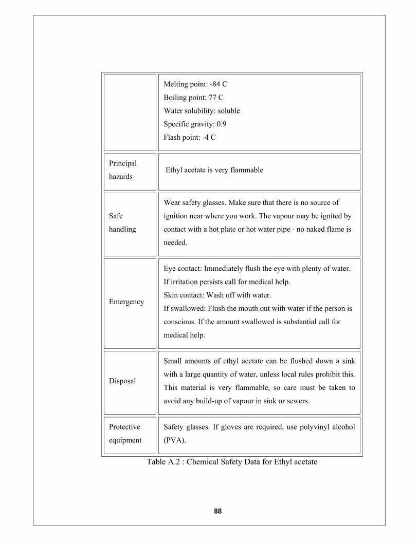
88
Melting point: -84 C
Boiling point: 77 C
Water solubility: soluble
Specific gravity: 0.9
Flash point: -4 C
Principal
hazards Ethyl acetate is very flammable
Safe
handling
Wear safety glasses. Make sure that there is no source of
ignition near where you work. The vapour may be ignited by
contact with a hot plate or hot water pipe - no naked flame is
needed.
Emergency
Eye contact: Immediately flush the eye with plenty of water.
If irritation persists call for medical help.
Skin contact: Wash off with water.
If swallowed: Flush the mouth out with water if the person is
conscious. If the amount swallowed is substantial call for
medical help.
Disposal
Small amounts of ethyl acetate can be flushed down a sink
with a large quantity of water, unless local rules prohibit this.
This material is very flammable, so care must be taken to
avoid any build-up of vapour in sink or sewers.
Protective
equipment
Safety glasses. If gloves are required, use polyvinyl alcohol
(PVA).
Table A.2 : Chemical Safety Data for Ethyl acetate
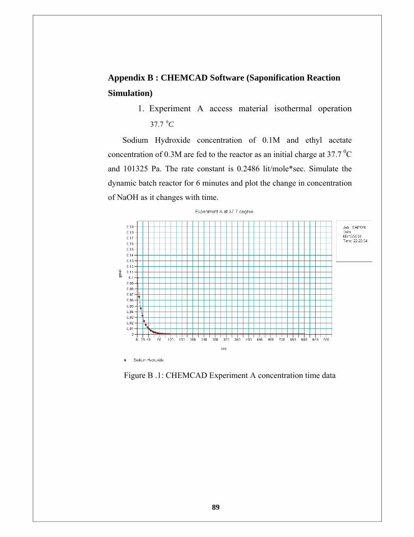
89
Appendix B : CHEMCAD Software (Saponification Reaction
Simulation)
1. Experiment A access material isothermal operation
C07.37
Sodium Hydroxide concentration of 0.1M and ethyl acetate
concentration of 0.3M are fed to the reactor as an initial charge at 37.7 0C
and 101325 Pa. The rate constant is 0.2486 lit/mole*sec. Simulate the
dynamic batch reactor for 6 minutes and plot the change in concentration
of NaOH as it changes with time.
Figure B .1: CHEMCAD Experiment A concentration time data
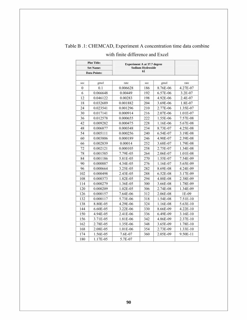
90
Table B .1: CHEMCAD, Experiment A concentration time data combine
with finite difference and Excel Plot Title:
Set Name:
Data Points:
Experiment A at 37.7 degree Sodium Hydroxide
61
sec gmol rate sec gmol rate
0 0.1 0.006628 186 8.76E-06 4.27E-07 6 0.066648 0.00449 192 6.57E-06 3.2E-07 12 0.046122 0.00283 198 4.92E-06 2.4E-07 18 0.032689 0.001882 204 3.69E-06 1.8E-07 24 0.023541 0.001296 210 2.77E-06 1.35E-07 30 0.017141 0.000914 216 2.07E-06 1.01E-07 36 0.012578 0.000655 222 1.55E-06 7.57E-08 42 0.009282 0.000475 228 1.16E-06 5.67E-08 48 0.006877 0.000348 234 8.73E-07 4.25E-08 54 0.005111 0.000256 240 6.54E-07 3.19E-08 60 0.003806 0.000189 246 4.90E-07 2.39E-08 66 0.002839 0.00014 252 3.68E-07 1.79E-08 72 0.002121 0.000105 258 2.75E-07 1.34E-08 78 0.001585 7.79E-05 264 2.06E-07 1.01E-08 84 0.001186 5.81E-05 270 1.55E-07 7.54E-09 90 0.000887 4.34E-05 276 1.16E-07 5.65E-09 96 0.000664 3.25E-05 282 8.69E-08 4.24E-09
102 0.000498 2.43E-05 288 6.52E-08 3.17E-09 108 0.000373 1.82E-05 294 4.88E-08 2.38E-09 114 0.000279 1.36E-05 300 3.66E-08 1.78E-09 120 0.000209 1.02E-05 306 2.74E-08 1.34E-09 126 0.000157 7.64E-06 312 2.06E-08 1E-09 132 0.000117 5.73E-06 318 1.54E-08 7.51E-10 138 8.80E-05 4.29E-06 324 1.16E-08 5.63E-10 144 6.60E-05 3.22E-06 330 8.66E-09 4.22E-10 150 4.94E-05 2.41E-06 336 6.49E-09 3.16E-10 156 3.71E-05 1.81E-06 342 4.86E-09 2.37E-10 162 2.78E-05 1.35E-06 348 3.65E-09 1.78E-10 168 2.08E-05 1.01E-06 354 2.73E-09 1.33E-10 174 1.56E-05 7.6E-07 360 2.05E-09 9.50E-11 180 1.17E-05 5.7E-07
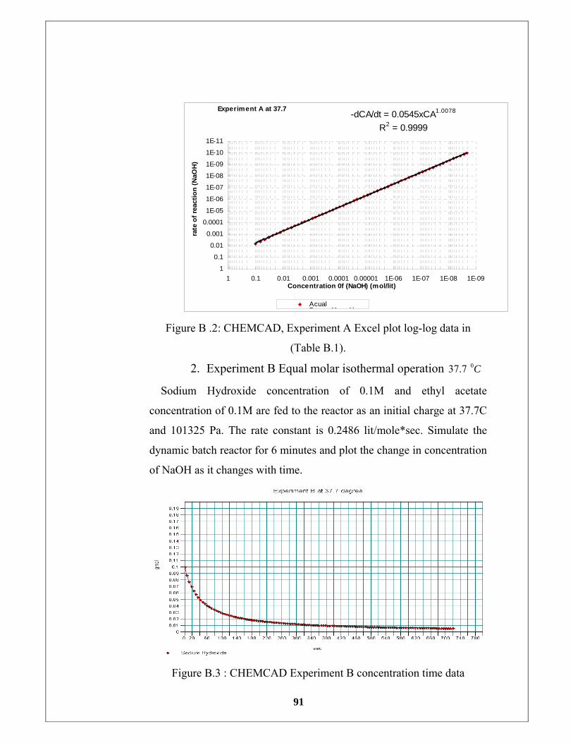
91
Experiment A at 37.7-dCA/dt = 0.0545xCA1.0078
R2 = 0.99991E-11
1E-10
1E-09
1E-08
1E-07
1E-06
1E-05
0.0001
0.001
0.01
0.1
11E-091E-081E-071E-060.000010.00010.0010.010.11
Concentration 0f (NaOH) (mol/lit)
rate
of r
eact
ion
(NaO
H)
Acual P (A l )
Figure B .2: CHEMCAD, Experiment A Excel plot log-log data in
(Table B.1).
2. Experiment B Equal molar isothermal operation C07.37
Sodium Hydroxide concentration of 0.1M and ethyl acetate
concentration of 0.1M are fed to the reactor as an initial charge at 37.7C
and 101325 Pa. The rate constant is 0.2486 lit/mole*sec. Simulate the
dynamic batch reactor for 6 minutes and plot the change in concentration
of NaOH as it changes with time.
Figure B.3 : CHEMCAD Experiment B concentration time data
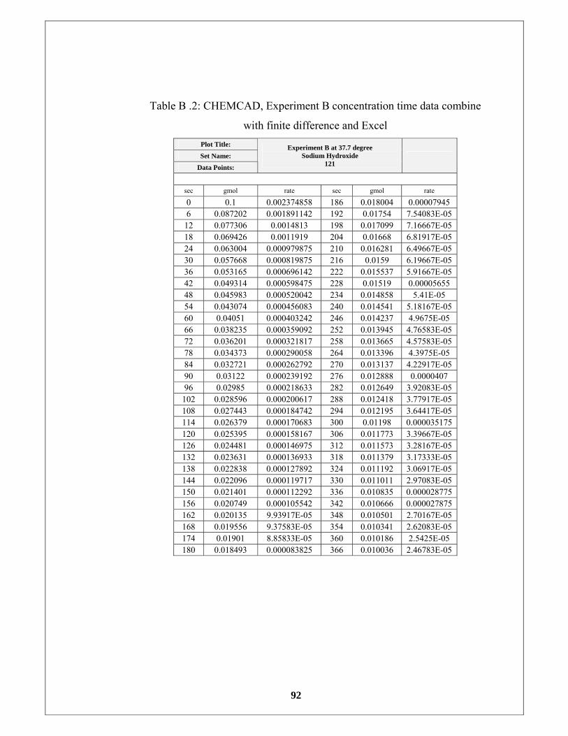
92
Table B .2: CHEMCAD, Experiment B concentration time data combine
with finite difference and Excel Plot Title:
Set Name:
Data Points:
Experiment B at 37.7 degree Sodium Hydroxide
121
sec gmol rate sec gmol rate
0 0.1 0.002374858 186 0.018004 0.00007945 6 0.087202 0.001891142 192 0.01754 7.54083E-05
12 0.077306 0.0014813 198 0.017099 7.16667E-05 18 0.069426 0.0011919 204 0.01668 6.81917E-05 24 0.063004 0.000979875 210 0.016281 6.49667E-05 30 0.057668 0.000819875 216 0.0159 6.19667E-05 36 0.053165 0.000696142 222 0.015537 5.91667E-05 42 0.049314 0.000598475 228 0.01519 0.00005655 48 0.045983 0.000520042 234 0.014858 5.41E-05 54 0.043074 0.000456083 240 0.014541 5.18167E-05 60 0.04051 0.000403242 246 0.014237 4.9675E-05 66 0.038235 0.000359092 252 0.013945 4.76583E-05 72 0.036201 0.000321817 258 0.013665 4.57583E-05 78 0.034373 0.000290058 264 0.013396 4.3975E-05 84 0.032721 0.000262792 270 0.013137 4.22917E-05 90 0.03122 0.000239192 276 0.012888 0.0000407 96 0.02985 0.000218633 282 0.012649 3.92083E-05 102 0.028596 0.000200617 288 0.012418 3.77917E-05 108 0.027443 0.000184742 294 0.012195 3.64417E-05 114 0.026379 0.000170683 300 0.01198 0.000035175 120 0.025395 0.000158167 306 0.011773 3.39667E-05 126 0.024481 0.000146975 312 0.011573 3.28167E-05 132 0.023631 0.000136933 318 0.011379 3.17333E-05 138 0.022838 0.000127892 324 0.011192 3.06917E-05 144 0.022096 0.000119717 330 0.011011 2.97083E-05 150 0.021401 0.000112292 336 0.010835 0.000028775 156 0.020749 0.000105542 342 0.010666 0.000027875 162 0.020135 9.93917E-05 348 0.010501 2.70167E-05 168 0.019556 9.37583E-05 354 0.010341 2.62083E-05 174 0.01901 8.85833E-05 360 0.010186 2.5425E-05 180 0.018493 0.000083825 366 0.010036 2.46783E-05
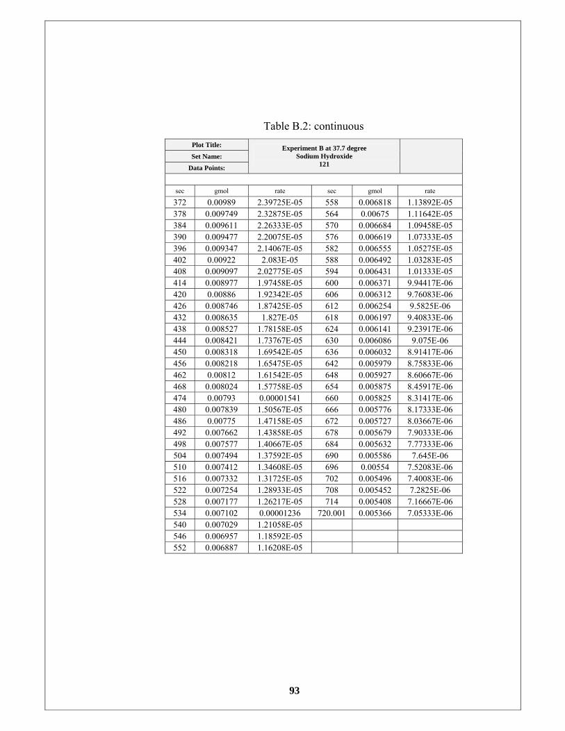
93
Table B.2: continuous Plot Title:
Set Name:
Data Points:
Experiment B at 37.7 degree Sodium Hydroxide
121
sec gmol rate sec gmol rate
372 0.00989 2.39725E-05 558 0.006818 1.13892E-05 378 0.009749 2.32875E-05 564 0.00675 1.11642E-05 384 0.009611 2.26333E-05 570 0.006684 1.09458E-05 390 0.009477 2.20075E-05 576 0.006619 1.07333E-05 396 0.009347 2.14067E-05 582 0.006555 1.05275E-05 402 0.00922 2.083E-05 588 0.006492 1.03283E-05 408 0.009097 2.02775E-05 594 0.006431 1.01333E-05 414 0.008977 1.97458E-05 600 0.006371 9.94417E-06 420 0.00886 1.92342E-05 606 0.006312 9.76083E-06 426 0.008746 1.87425E-05 612 0.006254 9.5825E-06 432 0.008635 1.827E-05 618 0.006197 9.40833E-06 438 0.008527 1.78158E-05 624 0.006141 9.23917E-06 444 0.008421 1.73767E-05 630 0.006086 9.075E-06 450 0.008318 1.69542E-05 636 0.006032 8.91417E-06 456 0.008218 1.65475E-05 642 0.005979 8.75833E-06 462 0.00812 1.61542E-05 648 0.005927 8.60667E-06 468 0.008024 1.57758E-05 654 0.005875 8.45917E-06 474 0.00793 0.00001541 660 0.005825 8.31417E-06 480 0.007839 1.50567E-05 666 0.005776 8.17333E-06 486 0.00775 1.47158E-05 672 0.005727 8.03667E-06 492 0.007662 1.43858E-05 678 0.005679 7.90333E-06 498 0.007577 1.40667E-05 684 0.005632 7.77333E-06 504 0.007494 1.37592E-05 690 0.005586 7.645E-06 510 0.007412 1.34608E-05 696 0.00554 7.52083E-06 516 0.007332 1.31725E-05 702 0.005496 7.40083E-06 522 0.007254 1.28933E-05 708 0.005452 7.2825E-06 528 0.007177 1.26217E-05 714 0.005408 7.16667E-06 534 0.007102 0.00001236 720.001 0.005366 7.05333E-06 540 0.007029 1.21058E-05 546 0.006957 1.18592E-05 552 0.006887 1.16208E-05
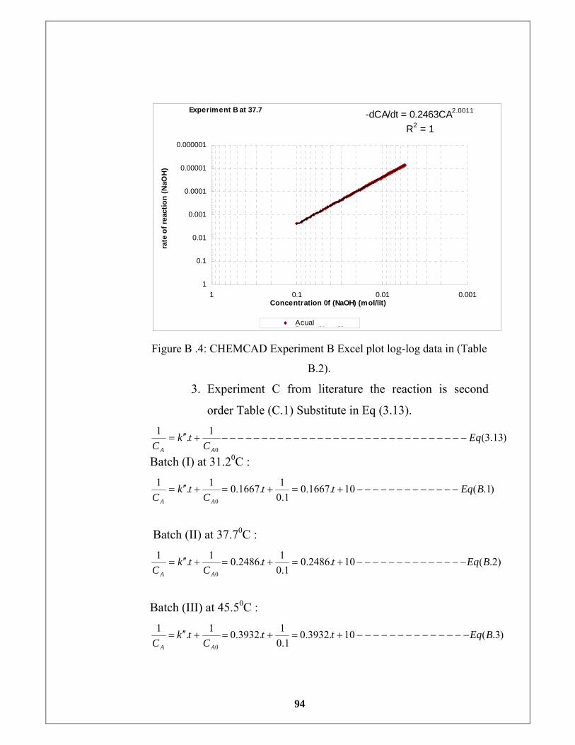
94
Experiment B at 37.7 -dCA/dt = 0.2463CA2.0011
R2 = 10.000001
0.00001
0.0001
0.001
0.01
0.1
10.0010.010.11
Concentration 0f (NaOH) (mol/lit)
rate
of r
eact
ion
(NaO
H)
Acual P (A l )
Figure B .4: CHEMCAD Experiment B Excel plot log-log data in (Table
B.2).
3. Experiment C from literature the reaction is second
order Table (C.1) Substitute in Eq (3.13).
)13.3(1.1
0
EqC
tkC AA
−−−−−−−−−−−−−−−−−−−−−−−−−−−−−−−+′′=
Batch (I) at 31.20C :
)1.(10.1667.01.0
1.1667.01.1
0
BEqttC
tkC AA
−−−−−−−−−−−−−+=+=+′′=
Batch (II) at 37.70C :
)2.(10.2486.01.0
1.2486.01.1
0
BEqttC
tkC AA
−−−−−−−−−−−−−−+=+=+′′=
Batch (III) at 45.50C :
)3.(10.3932.01.0
1.3932.01.1
0
BEqttC
tkC AA
−−−−−−−−−−−−−−+=+=+′′=
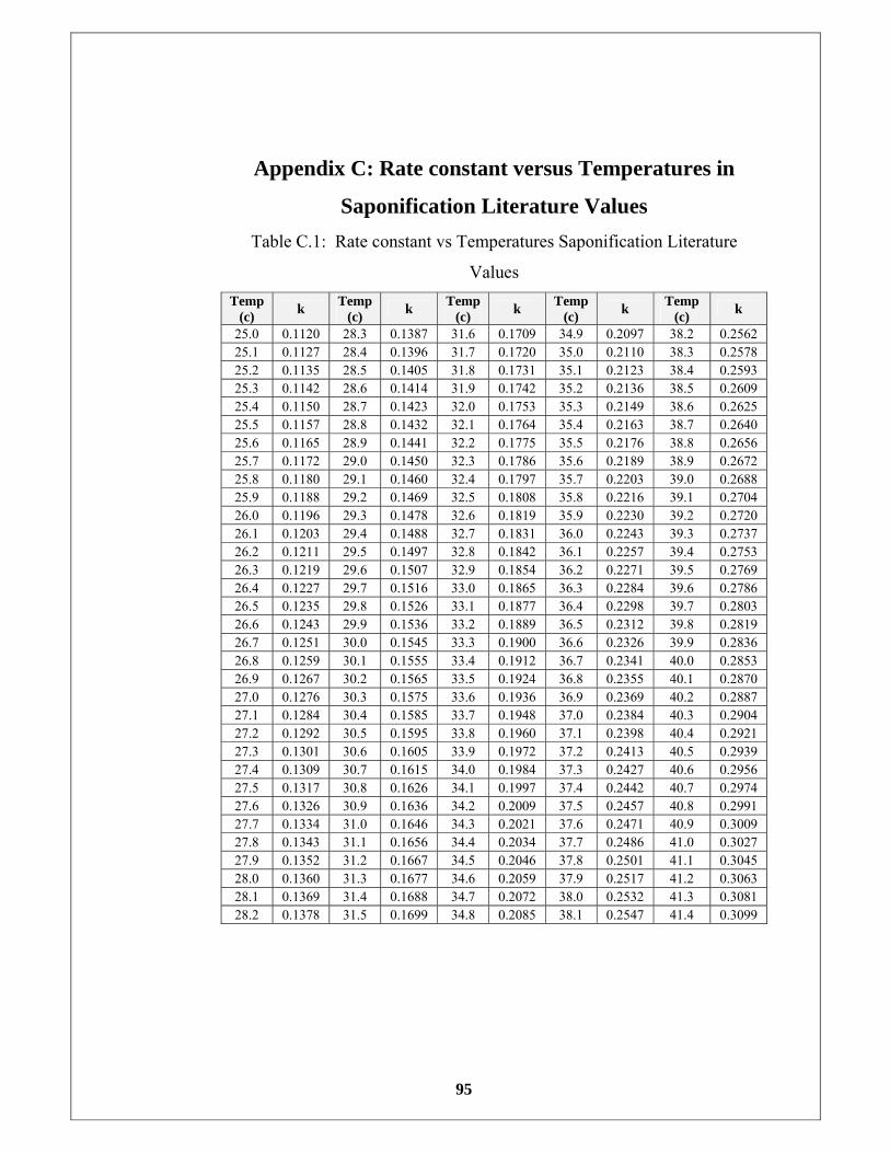
95
Appendix C: Rate constant versus Temperatures in
Saponification Literature Values Table C.1: Rate constant vs Temperatures Saponification Literature
Values Temp
(c) k Temp (c) k Temp
(c) k Temp (c) k Temp
(c) k
25.0 0.1120 28.3 0.1387 31.6 0.1709 34.9 0.2097 38.2 0.2562 25.1 0.1127 28.4 0.1396 31.7 0.1720 35.0 0.2110 38.3 0.2578 25.2 0.1135 28.5 0.1405 31.8 0.1731 35.1 0.2123 38.4 0.2593 25.3 0.1142 28.6 0.1414 31.9 0.1742 35.2 0.2136 38.5 0.2609 25.4 0.1150 28.7 0.1423 32.0 0.1753 35.3 0.2149 38.6 0.2625 25.5 0.1157 28.8 0.1432 32.1 0.1764 35.4 0.2163 38.7 0.2640 25.6 0.1165 28.9 0.1441 32.2 0.1775 35.5 0.2176 38.8 0.2656 25.7 0.1172 29.0 0.1450 32.3 0.1786 35.6 0.2189 38.9 0.2672 25.8 0.1180 29.1 0.1460 32.4 0.1797 35.7 0.2203 39.0 0.2688 25.9 0.1188 29.2 0.1469 32.5 0.1808 35.8 0.2216 39.1 0.2704 26.0 0.1196 29.3 0.1478 32.6 0.1819 35.9 0.2230 39.2 0.2720 26.1 0.1203 29.4 0.1488 32.7 0.1831 36.0 0.2243 39.3 0.2737 26.2 0.1211 29.5 0.1497 32.8 0.1842 36.1 0.2257 39.4 0.2753 26.3 0.1219 29.6 0.1507 32.9 0.1854 36.2 0.2271 39.5 0.2769 26.4 0.1227 29.7 0.1516 33.0 0.1865 36.3 0.2284 39.6 0.2786 26.5 0.1235 29.8 0.1526 33.1 0.1877 36.4 0.2298 39.7 0.2803 26.6 0.1243 29.9 0.1536 33.2 0.1889 36.5 0.2312 39.8 0.2819 26.7 0.1251 30.0 0.1545 33.3 0.1900 36.6 0.2326 39.9 0.2836 26.8 0.1259 30.1 0.1555 33.4 0.1912 36.7 0.2341 40.0 0.2853 26.9 0.1267 30.2 0.1565 33.5 0.1924 36.8 0.2355 40.1 0.2870 27.0 0.1276 30.3 0.1575 33.6 0.1936 36.9 0.2369 40.2 0.2887 27.1 0.1284 30.4 0.1585 33.7 0.1948 37.0 0.2384 40.3 0.2904 27.2 0.1292 30.5 0.1595 33.8 0.1960 37.1 0.2398 40.4 0.2921 27.3 0.1301 30.6 0.1605 33.9 0.1972 37.2 0.2413 40.5 0.2939 27.4 0.1309 30.7 0.1615 34.0 0.1984 37.3 0.2427 40.6 0.2956 27.5 0.1317 30.8 0.1626 34.1 0.1997 37.4 0.2442 40.7 0.2974 27.6 0.1326 30.9 0.1636 34.2 0.2009 37.5 0.2457 40.8 0.2991 27.7 0.1334 31.0 0.1646 34.3 0.2021 37.6 0.2471 40.9 0.3009 27.8 0.1343 31.1 0.1656 34.4 0.2034 37.7 0.2486 41.0 0.3027 27.9 0.1352 31.2 0.1667 34.5 0.2046 37.8 0.2501 41.1 0.3045 28.0 0.1360 31.3 0.1677 34.6 0.2059 37.9 0.2517 41.2 0.3063 28.1 0.1369 31.4 0.1688 34.7 0.2072 38.0 0.2532 41.3 0.3081 28.2 0.1378 31.5 0.1699 34.8 0.2085 38.1 0.2547 41.4 0.3099
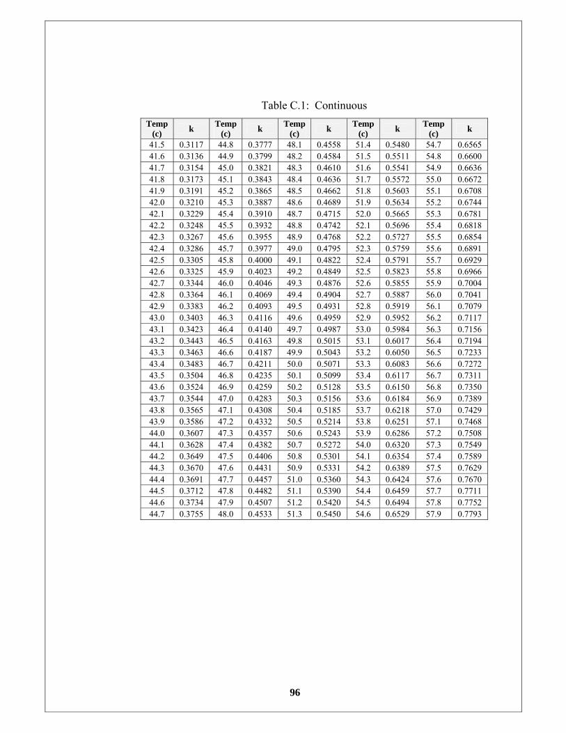
96
Table C.1: Continuous Temp
(c) k Temp (c) k Temp
(c) k Temp (c) k Temp
(c) k
41.5 0.3117 44.8 0.3777 48.1 0.4558 51.4 0.5480 54.7 0.6565 41.6 0.3136 44.9 0.3799 48.2 0.4584 51.5 0.5511 54.8 0.6600 41.7 0.3154 45.0 0.3821 48.3 0.4610 51.6 0.5541 54.9 0.6636 41.8 0.3173 45.1 0.3843 48.4 0.4636 51.7 0.5572 55.0 0.6672 41.9 0.3191 45.2 0.3865 48.5 0.4662 51.8 0.5603 55.1 0.6708 42.0 0.3210 45.3 0.3887 48.6 0.4689 51.9 0.5634 55.2 0.6744 42.1 0.3229 45.4 0.3910 48.7 0.4715 52.0 0.5665 55.3 0.6781 42.2 0.3248 45.5 0.3932 48.8 0.4742 52.1 0.5696 55.4 0.6818 42.3 0.3267 45.6 0.3955 48.9 0.4768 52.2 0.5727 55.5 0.6854 42.4 0.3286 45.7 0.3977 49.0 0.4795 52.3 0.5759 55.6 0.6891 42.5 0.3305 45.8 0.4000 49.1 0.4822 52.4 0.5791 55.7 0.6929 42.6 0.3325 45.9 0.4023 49.2 0.4849 52.5 0.5823 55.8 0.6966 42.7 0.3344 46.0 0.4046 49.3 0.4876 52.6 0.5855 55.9 0.7004 42.8 0.3364 46.1 0.4069 49.4 0.4904 52.7 0.5887 56.0 0.7041 42.9 0.3383 46.2 0.4093 49.5 0.4931 52.8 0.5919 56.1 0.7079 43.0 0.3403 46.3 0.4116 49.6 0.4959 52.9 0.5952 56.2 0.7117 43.1 0.3423 46.4 0.4140 49.7 0.4987 53.0 0.5984 56.3 0.7156 43.2 0.3443 46.5 0.4163 49.8 0.5015 53.1 0.6017 56.4 0.7194 43.3 0.3463 46.6 0.4187 49.9 0.5043 53.2 0.6050 56.5 0.7233 43.4 0.3483 46.7 0.4211 50.0 0.5071 53.3 0.6083 56.6 0.7272 43.5 0.3504 46.8 0.4235 50.1 0.5099 53.4 0.6117 56.7 0.7311 43.6 0.3524 46.9 0.4259 50.2 0.5128 53.5 0.6150 56.8 0.7350 43.7 0.3544 47.0 0.4283 50.3 0.5156 53.6 0.6184 56.9 0.7389 43.8 0.3565 47.1 0.4308 50.4 0.5185 53.7 0.6218 57.0 0.7429 43.9 0.3586 47.2 0.4332 50.5 0.5214 53.8 0.6251 57.1 0.7468 44.0 0.3607 47.3 0.4357 50.6 0.5243 53.9 0.6286 57.2 0.7508 44.1 0.3628 47.4 0.4382 50.7 0.5272 54.0 0.6320 57.3 0.7549 44.2 0.3649 47.5 0.4406 50.8 0.5301 54.1 0.6354 57.4 0.7589 44.3 0.3670 47.6 0.4431 50.9 0.5331 54.2 0.6389 57.5 0.7629 44.4 0.3691 47.7 0.4457 51.0 0.5360 54.3 0.6424 57.6 0.7670 44.5 0.3712 47.8 0.4482 51.1 0.5390 54.4 0.6459 57.7 0.7711 44.6 0.3734 47.9 0.4507 51.2 0.5420 54.5 0.6494 57.8 0.7752 44.7 0.3755 48.0 0.4533 51.3 0.5450 54.6 0.6529 57.9 0.7793


![Process Intensification - AIChE€¦ · Process Intensification Adam Harvey ... Case Study: A Saponification reaction in ... 375 m3 Batch Reactor [50 m fill]](https://img.pdfslide.net/doc/110x75/5ae67ea17f8b9a6d4f8ccd69/process-intensification-process-intensification-adam-harvey-case-study.jpg)