SANDIA REPORT SAND2006-5855 Unlimited Release Printed September 2006

SAR Processing with Stepped Chirps and Phased Array Antennas Armin W. Doerry Prepared by Sandia National Laboratories Albuquerque, New Mexico 87185 and Livermore, California 94550 Sandia is a multiprogram laboratory operated by Sandia Corporation, a Lockheed Martin Company, for the United States Department of Energy’s National Nuclear Security Administration under Contract DE-AC04-94AL85000. Approved for public release; further dissemination unlimited.

- 2 -

Issued by Sandia National Laboratories, operated for the United States Department of Energy by Sandia Corporation. NOTICE: This report was prepared as an account of work sponsored by an agency of the United States Government. Neither the United States Government, nor any agency thereof, nor any of their employees, nor any of their contractors, subcontractors, or their employees, make any warranty, express or implied, or assume any legal liability or responsibility for the accuracy, completeness, or usefulness of any information, apparatus, product, or process disclosed, or represent that its use would not infringe privately owned rights. Reference herein to any specific commercial product, process, or service by trade name, trademark, manufacturer, or otherwise, does not necessarily constitute or imply its endorsement, recommendation, or favoring by the United States Government, any agency thereof, or any of their contractors or subcontractors. The views and opinions expressed herein do not necessarily state or reflect those of the United States Government, any agency thereof, or any of their contractors. Printed in the United States of America. This report has been reproduced directly from the best available copy. Available to DOE and DOE contractors from U.S. Department of Energy Office of Scientific and Technical Information P.O. Box 62 Oak Ridge, TN 37831 Telephone: (865) 576-8401 Facsimile: (865) 576-5728 E-Mail: reports@adonis.osti.gov Online ordering: http://www.osti.gov/bridge Available to the public from U.S. Department of Commerce National Technical Information Service 5285 Port Royal Rd. Springfield, VA 22161 Telephone: (800) 553-6847 Facsimile: (703) 605-6900 E-Mail: orders@ntis.fedworld.gov Online order: http://www.ntis.gov/help/ordermethods.asp?loc=7-4-0#online

SAND2006-5855 Unlimited Release

Printed September 2006

SAR Processing with Stepped Chirps and Phased Array Antennas

Armin W. Doerry

SAR Applications Department

Sandia National Laboratories PO Box 5800

Albuquerque, NM 87185-1330

ABSTRACT Wideband radar signals are problematic for phased array antennas. Wideband radar signals can be generated from series or groups of narrow-band signals centered at different frequencies. An equivalent wideband LFM chirp can be assembled from lesser-bandwidth chirp segments in the data processing. The chirp segments can be transmitted as separate narrow-band pulses, each with their own steering phase operation. This overcomes the problematic dilemma of steering wideband chirps with phase shifters alone, that is, without true time-delay elements.

- 3 -

ACKNOWLEDGEMENTS This work was funded by the US DOE Office of Nonproliferation & National Security, Office of Research and Development, NA-22, under the Advanced Radar System (ARS) project.

Sandia is a multiprogram laboratory operated by Sandia Corporation, a Lockheed Martin Company, for the United States Department of Energy under Contract DE-AC04- 94AL85000.

- 4 -

CONTENTS FOREWORD.................................................................................................................................................. 6 1 Introduction & Background..................................................................................................................... 7 2 Overview & Summary............................................................................................................................. 9 3 Detailed Analysis .................................................................................................................................. 11

3.1 The video phase history data model ............................................................................................... 11 3.2 Stepped Chirps ............................................................................................................................... 17 3.3 Phased Array Limitations............................................................................................................... 21 3.4 Parameter Selection........................................................................................................................ 24

4 Conclusions ........................................................................................................................................... 25 REFERENCES............................................................................................................................................. 27 DISTRIBUTION.......................................................................................................................................... 30

- 5 -

FOREWORD The underlying problem addressed in this report is “How do we make a phased array antenna perform fine-resolution SAR in squinted geometries?” The hang-up is that steering wideband signals really requires true time-delay adjustments between antenna array elements, but phase shifters are much easier to implement.

Nevertheless, the advent of Sandia’s MiniSAR has sparked a new round of interest from multiple companies and agencies in marrying the MiniSAR to their phased array antenna system, which invariably employs phase shifters, and not true time-delay adjustments.

Herein we propose a solution that has its origins in another program, the DOE NA-22 funded Concealed Target SAR (CTSAR) project, where it was briefly investigated the concept of coherently combining data taken at different portions of the radar band that in the case of CTSAR needed to omit specific stay-out frequencies. Ultimately, however, this was not employed in the CTSAR project.

For the current phased array antenna effort, the bands are adjacent, but need to be transmitted separately for other reasons, namely to allow independent adjustment of phase shifters in the phased array antenna system.

- 6 -

1 Introduction & Background Conventional Synthetic Aperture Radar (SAR) achieves its range resolution from the bandwidth of its transmitted signal, and its azimuth resolution from the diversity of its viewing aspect angle. Typically, at any one location along its synthetic aperture, the radar transmits a pulse that exhibits the entire bandwidth of interest. Often this is a Linear Frequency Modulated (LFM) chirp signal, although other modulation schemes may also provide the bandwidth necessary to achieve the desired resolution.

The raw echo data that is collected by the radar is termed the Phase-History data, or just Phase Histories. LFM Phase History data that is dechirped, in a technique known as stretch processing,1 are effectively holograms of the scene being imaged, that is, samples of the Fourier Space of the scene. This data can be processed into an image using transform techniques. A common technique for fine resolution processing is the Polar Format Algorithm (PFA) processing technique, first presented by Walker,2 but since described by many others. Other algorithms and techniques also exist, and other waveforms may also be manipulated with relatively simple signal processing to represent the Fourier space of the scene.

Two recent technology developments have come on the scene with conflicting demands on the radar.

The first is the advent of extremely fine-resolution multi-mode SAR systems, often exhibiting resolutions on the order of 0.1 m or less. Operationally, these SAR systems are required to be able to squint substantially forward or aft of broadside to the aircraft, perhaps by 45 degrees or more. Nevertheless, the fine resolutions require transmitted signal bandwidths of many hundreds of MHz, even approaching 2 GHz for 0.1 m resolution after sidelobe filtering.

The second development that conflicts with the first is the advent of applications necessitating Active Electronically Steered [phased] Array (AESA) antenna technology. These systems rely on steering the antenna beam by adjusting the phase and/or delay of signals applied to individual radiating elements, or sometimes small groups of radiating elements. The ‘cleanest’ steering technique is to provide time delay between elements, but for relatively narrow-band signals this is approximated by adjusting the phase between elements. For narrow-band signals these are essentially equivalent techniques. Phase shifters are generally easier and less costly to implement than programmable true time-delay elements. The down-side is that phase shifters are problematic for steering wideband signals, such as those required by fine-resolution SAR systems.

Essentially, the required time delay requires a frequency-dependent phase shift. Approximating a time delay with a constant phase shift is tolerable for narrow-band signals, but not for wideband signals. Hence the conflicting demands for fine-resolution inexpensive AESA based SAR.

- 7 -

Skolnik3 presents a rule-of-thumb for the threshold of tolerance while employing only phase shifters is that at a 60 degree scan angle,

( ) ( )degbeamwidthboresight%Bandwidth ≈ .

The object of this report is to describe a technique whereby a wideband LFM chirp is broken into several segments, with each relatively narrow-band segment transmitted on a separate pulse, and capable of being adequately steered by phase shifters in an AESA.

Prior Art

Alberti, et al.,4 describe their MINISAR radar system that employs a stepped chirp signal for the purpose of adding “flexibility to the system that can be easily upgraded to transmit wider bandwidth,” and allowing “the use of more precise chirp generator devices able to assure high degree of phase linearity.” Their system is nevertheless fairly narrow-band in that it offers 280 MHz of resolution bandwidth at X-band, achieved in four 70 MHz consecutive chirp segments. Furthermore, while they employ an array antenna, it is not an AESA.

Schimpf, et al.,5 describe a short-range millimeter-wave SAR system that uses segmented LFM waveforms for the purpose of limiting chirp rate in spite of extremely short pulses used. No mention of phased array beam steering issues are made. This system is further described by Brehm, et al.6

Yunhua, et al.,7 discuss processing stepped chirp signals, but do not address phased array antennas at all.

Narayanan, et al.,8 also describe what they call a “stepped-chirp frequency modulation (SCFM) radar.” However this radar creates a single waveform that is chirped by applying a digitally sampled ramp to a Voltage Controlled Oscillator, creating that chirp in a stepped fashion. This is apparently done uniformly to each pulse. Furthermore, although an array antenna is used, it is not an AESA.

Some systems described as step-chirp systems in fact operate by synthesizing a chirp via transmitting a single frequency with each pulse, but varying that frequency on a pulse-to-pulse basis. Tuley, et al.,9 describe such a system.

Weiss, et al.,10 describe a wideband SAR employing an AESA. However, they observe “the need of true time delays to guarantee the aspired range resolution of one decimeter also for large squint angles.”

Pape and Goutzoulis11 describe a photonic true time-delay element for wideband phased array antennas, stating that such devices are required “[t]o satisfy the simultaneous requirements of wide bandwidth and large antenna scan angle.”

Loo, et al.,12 also describe using photonics to implement true time-delay for AESA beam steering to avoid “beam squint.”

- 8 -

Goutzoulis, et al.13, describe a hybrid electronic and fiber optic true time-delay circuit for AESA application, and in the process acknowledge that electronic solutions offer “economical advantages.”

Fischman, et al.,14 describe a hybrid approach to AESA beam steering that involves phase shifters, and both analog and digital true time-delay elements. This is for a large (50 m x 2 m) L-band antenna even with signals of only 80 MHz bandwidth.

Schuss & Hanfling15 were issued a patent where “[a] space fed antenna system is adapted to correct for beam pointing (squint) errors and collimation errors caused by frequency variations of the R.F. energy radiated by the antenna system.” Their technique requires time-delay elements for wideband signals.

Boe, et al.,16 were issued a patent in 2004 “for maintaining beam pointing (also known as stabilizing) for an Electronically Scanned Antenna (ESA) as its frequency is varied over a wide frequency bandwidth. The technique uses discrete phase shifters, a number of stored states, and a control methodology for rapidly switching among the states, e.g. within a pulse.” The concept of rapidly adjusting phase shifters within a chirped pulse requires overhead in circuitry that may be problematic to efficient low-cost system design and manufacture.

An interesting side-note is that the feature of scan angle changing with frequency is actually employed to advantage in a class of radars called “Frequency-Scan Arrays”, as noted by Skolnik.17

2 Overview & Summary Fine resolution SAR requires wideband signals to be transmitted and received. Electronically steered phased-array antennas have difficulty steering wideband signals without the use of expensive and cumbersome true time delay elements. More desirable phase shifters are by themselves inadequate to the task.

Wideband radar signals can be generated from series or groups of narrow-band signals centered at different frequencies. A wideband LFM chirp can be assembled from lesser-bandwidth chirp segments. The chirp segments can be transmitted as separate pulses, each with their own steering phase operation. The chirp segment bandwidth would essentially be narrow-band by itself. This overcomes the problematic dilemma of steering wideband chirps with phase shifters alone. True time-delay elements are not required.

- 9 -

“I have never let my schooling interfere with my education.”

Mark Twain

- 10 -

3 Detailed Analysis

3.1 The video phase history data model Consider a LFM transmitted signal of the form

( ) ( ) ( )⎭⎬⎫

⎩⎨⎧

−+−+⎟⎠⎞

⎜⎝⎛ −

= 2,,, 2

exprect, nnT

nnTnTn

TT ttttjT

ttAntX

γωφ (1)

where

TA = the amplitude of the transmitted pulse, = time, = index value of pulse number,

tn 22 NnN <≤− ,

= reference time of nth pulse, = transmitted pulse width,

ntT

nT ,φ = transmit waveform reference phase of nth pulse,

nT ,ω = transmit waveform reference frequency of nth pulse, and

nT ,γ = transmit waveform chirp rate of nth pulse. (2)

The received echo from a point scatterer is a delayed and attenuated version of this, namely

( ) ( nttXAA

ntX nsTT

RR ,, ,−= )

t

(3)

where

RA = the amplitude of the received pulse, = echo delay time of the received echo for the nth pulse. (4) ns,

This is expanded to

( ) ( ) ( )⎭⎬⎫

⎩⎨⎧

−−+−−+⎟⎟⎠

⎞⎜⎜⎝

⎛ −−= 2

,,

,,,,

2exprect, nsn

nTnsnnTnT

nsnRR ttttttj

Tttt

AntXγ

ωφ .

(5)

Employing stretch processing, and Quadrature demodulation, requires mixing this with a Local Oscillator (LO) signal of the form

- 11 -

( ) ( ) ( )⎭⎬⎫

⎩⎨⎧

−−+−−+⎟⎟⎠

⎞⎜⎜⎝

⎛ −−= 2

,,

,,,,

2exprect, nmn

nLnmnnLnL

L

nmnL ttttttj

Tttt

ntXγ

ωφ

(6)

where

nmt , = reference delay time of nth LO pulse, = LO pulse width, LT

nL,φ = LO waveform reference phase of nth LO pulse,

nL,ω = LO waveform reference frequency of nth LO pulse, and

nL,γ = LO waveform chirp rate of nth LO pulse. (7)

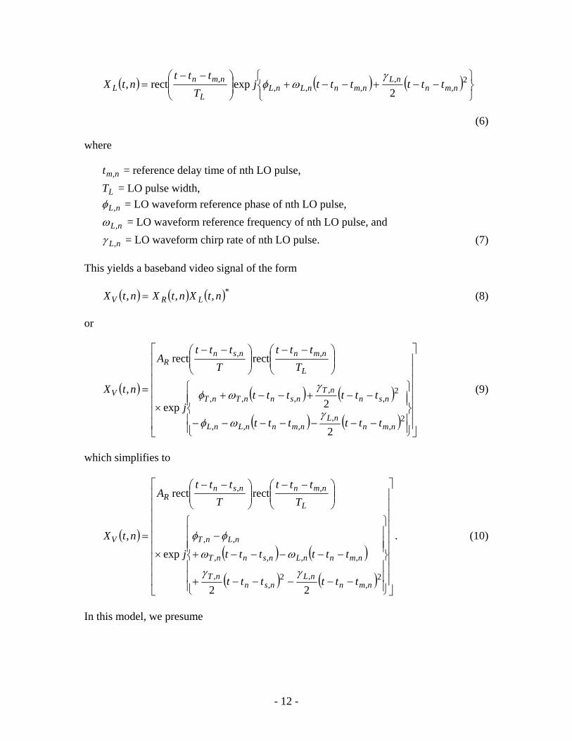
This yields a baseband video signal of the form

( ) ( ) ( )*,,, ntXntXntX LRV = (8)

or

( ) ( ) ( )

( ) ( ) ⎥⎥⎥⎥⎥⎥⎥

⎦

⎤

⎢⎢⎢⎢⎢⎢⎢

⎣

⎡

⎪⎪⎭

⎪⎪⎬

⎫

⎪⎪⎩

⎪⎪⎨

⎧

−−−−−−−

−−+−−+×

⎟⎟⎠

⎞⎜⎜⎝

⎛ −−⎟⎟⎠

⎞⎜⎜⎝

⎛ −−

=

2,

,,,,

2,

,,,,

,,

2

2exp

rectrect

,

nmnnL

nmnnLnL

nsnnT

nsnnTnT

L

nmnnsnR

V

tttttt

ttttttj

Tttt

Tttt

A

ntX

γωφ

γωφ (9)

which simplifies to

( )( ) ( )

( ) ( ) ⎥⎥⎥⎥⎥⎥⎥⎥⎥

⎦

⎤

⎢⎢⎢⎢⎢⎢⎢⎢⎢

⎣

⎡

⎪⎪⎪

⎭

⎪⎪⎪

⎬

⎫

⎪⎪⎪

⎩

⎪⎪⎪

⎨

⎧

−−−−−+

−−−−−+

−

×

⎟⎟⎠

⎞⎜⎜⎝

⎛ −−⎟⎟⎠

⎞⎜⎜⎝

⎛ −−

=

2,

,2,

,

,,,,

,,

,,

22

exp

rectrect

,

nmnnL

nsnnT

nmnnLnsnnT

nLnT

L

nmnnsnR

V

tttttt

ttttttj

Tttt

Tttt

A

ntX

γγ

ωω

φφ . (10)

In this model, we presume

- 12 -

nTnL ,, φφ = ,

nTnL ,, ωω = ,

nTnL ,, , (11) γγ =

which allows the reduction to

( )( )( )( ) ( )

⎥⎥⎥⎥⎥

⎦

⎤

⎢⎢⎢⎢⎢

⎣

⎡

⎭⎬⎫

⎩⎨⎧

−+−−−+×

⎟⎟⎠

⎞⎜⎜⎝

⎛ −−⎟⎠⎞

⎜⎝⎛ −−

=2,

,, 2exp

rectrect,

smnT

smmnnTnT

L

mnsnR

V

tttttttj

Tttt

TtttA

ntXγ

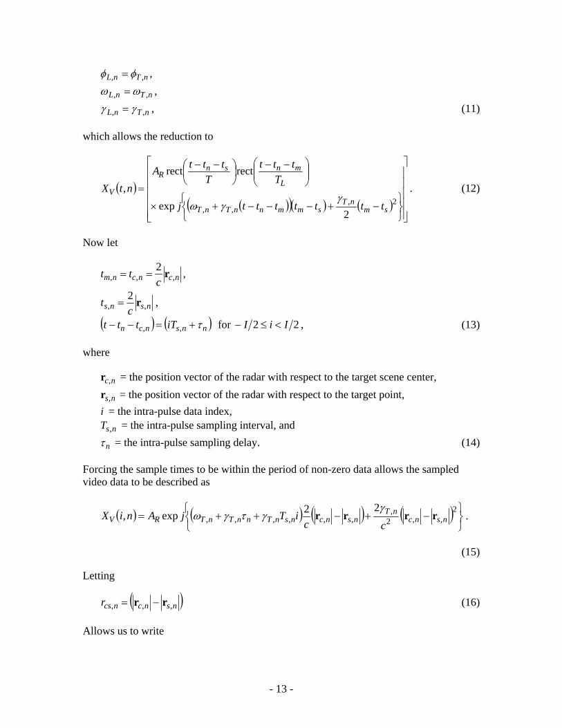
γω. (12)

Now let

ncncnm ctt ,,,

2 r== ,

nsns ct ,, r=

2 ,

( ) ( )nnsncn iTttt τ+=−− ,, for 22 IiI <≤− , (13)

where

nc,r = the position vector of the radar with respect to the target scene center, = the position vector of the radar with respect to the target point,

= the intra-pulse data index, = the intra-pulse sampling interval, and

ns,ri

,nsT

nτ = the intra-pulse sampling delay. (14)

Forcing the sample times to be within the period of non-zero data allows the sampled video data to be described as

( ) ( ) ( ) ( )⎭⎬⎫

⎩⎨⎧

−+−++=2

,,2,

,,,,,,22exp, nsnc

nTnsncnsnTnnTnTRV cc

iTjAniX rrrrγ

γτγω .

(15)

Letting

( )nsncncsr ,,, rr −= (16)

Allows us to write

- 13 -

( ) ( )⎭⎬⎫

⎩⎨⎧

+++= 2,2

,,,,,,

22exp, ncsnT

ncsnsnTnnTnTRV rc

rc

iTjAniXγ

γτγω . (17)

It becomes convenient to constrain

( ) ( )iTiT snnsnTnnTnT 0,00,,,, γωκγτγω +=++ (18)

where

0ω = the nominal or reference frequency,

0γ = the nominal or reference chirp rate, and = the nominal or reference sample spacing, (19) 0,sT

which allows

( ) ( )⎭⎬⎫

⎩⎨⎧

++= 2,2

,,0,00

22exp, ncsnT

ncsnsRV rc

riTc

jAniXγ

κγω . (20)

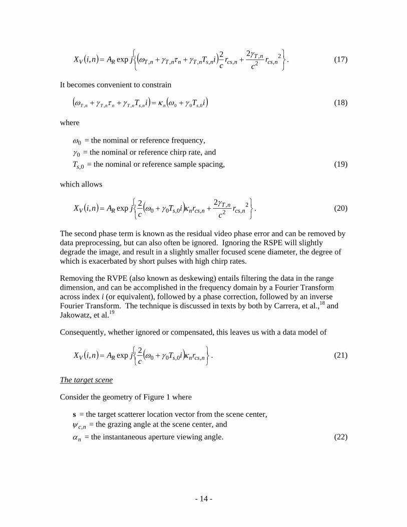
The second phase term is known as the residual video phase error and can be removed by data preprocessing, but can also often be ignored. Ignoring the RSPE will slightly degrade the image, and result in a slightly smaller focused scene diameter, the degree of which is exacerbated by short pulses with high chirp rates.

Removing the RVPE (also known as deskewing) entails filtering the data in the range dimension, and can be accomplished in the frequency domain by a Fourier Transform across index i (or equivalent), followed by a phase correction, followed by an inverse Fourier Transform. The technique is discussed in texts by both by Carrera, et al.,18 and Jakowatz, et al.19

Consequently, whether ignored or compensated, this leaves us with a data model of

( ) ( )⎭⎬⎫

⎩⎨⎧ += ncsnsRV riT

cjAniX ,0,00

2exp, κγω . (21)

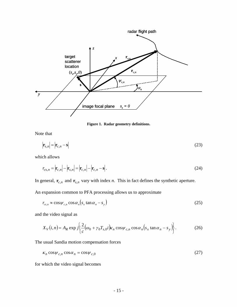
The target scene

Consider the geometry of Figure 1 where

s = the target scatterer location vector from the scene center, nc,ψ = the grazing angle at the scene center, and

nα = the instantaneous aperture viewing angle. (22)

- 14 -

radar flight path

rc,n

rs,n

s

target scattererlocation

(sx,sy,0)

x

z

y

image focal plane sz = 0

ψc,n

αn

radar flight path

rc,n

rs,n

s

target scattererlocation

(sx,sy,0)

x

z

y

image focal plane sz = 0

ψc,n

αn

Figure 1. Radar geometry definitions.

Note that

srr −= ncns ,, (23)

which allows

srrrr −−=−= ncncnsncncsr ,,,,, . (24)

In general, and vary with index n. This in fact defines the synthetic aperture. nc,r ns,r

An expansion common to PFA processing allows us to approximate

( )ynxnncncs ssr −≈ ααψ tancoscos ,, (25)

and the video signal as

( ) ( ) (⎭⎬⎫

⎩⎨⎧ −+= ynxnncnsRV ssiT

cjAniX ααψκγω tancoscos2exp, ,0,00 ) . (26)

The usual Sandia motion compensation forces

0,, coscoscos cnncn ψαψκ = (27)

for which the video signal becomes

- 15 -

( ) ( ) (⎭⎬⎫

⎩⎨⎧ −+= ynxcsRV ssiT

cjAniX αψγω tancos2exp, 0,0,00 ) . (28)

In more conventional systems, this is accomplished with data resampling and interpolation, but achieves the same result.

Spatial sample points are conveniently chosen at

ndn αα =tan (29)

so that the final model becomes

( ) ( ) (⎭⎬⎫

⎩⎨⎧ −+= yxcsRV sndsiT

cjAniX αψγω 0,0,00 cos2exp, ) . (30)

This is our generalized starting point, consistent with current Sandia data collection and processing techniques.

PFA Processing

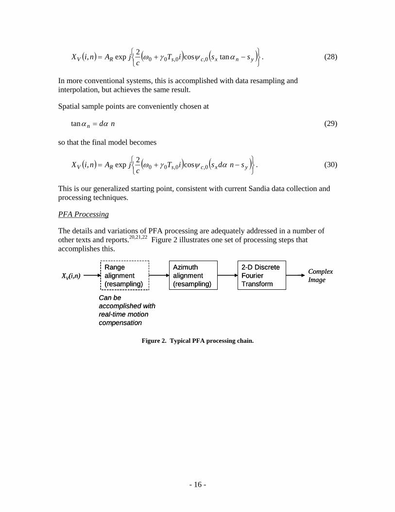
The details and variations of PFA processing are adequately addressed in a number of other texts and reports.20, ,21 22 Figure 2 illustrates one set of processing steps that accomplishes this.

Range alignment (resampling)

Azimuth alignment (resampling)

2-D Discrete Fourier Transform

XV(i,n) ComplexImage

Can be accomplished with real-time motion compensation

Range alignment (resampling)

Azimuth alignment (resampling)

2-D Discrete Fourier Transform

XV(i,n) ComplexImage

Can be accomplished with real-time motion compensation

Figure 2. Typical PFA processing chain.

- 16 -

3.2 Stepped Chirps The idea becomes to transmit only a small segment of the entire bandwidth on any one pulse, moving that segment’s center frequency on a pulse to pulse basis, thereby covering the entire resolution bandwidth with multiple pulses.

First we divide the sample set of index n into P subapertures or groups of width M pulses each, such that

pMmn += (31)

where

m = the segment intra-group azimuth index, 22 MmM <≤− , and = the inter-group azimuth index, p 22 PpP <≤− . (32)

Note that with no overlap, this implies that

MPN = . (33)

The concept of segmented chirps implies a constraint on the range of index i for particular segment positions m, such that

mKki += (34)

where

k = the segment range index, 22 KkK <≤− . (35)

That is, each pulse collects K samples using some lesser-bandwidth chirp.

With no overlap, this implies that

MKI = . (36)

The video signal model becomes

( ) ( )( ) ( )( )⎭⎬⎫

⎩⎨⎧ −+++= yxcsRV spMmdsmKkT

cjAmpkX αψγω 0,0,00 cos2exp,, (37)

which we manipulate to

( ) ( )( ) ⎪⎭

⎪⎬⎫

⎪⎩

⎪⎨⎧

−+×

++=

yxx

cssRV

smdsMpds

kTKmTcjAmpkX

αα

ψγγω 0,0,00,00 cos2exp,, . (38)

- 17 -

Some observations are worth noting.

For a specific pulse, that is, a particular chirp segment within a particular group, the values for indices p and m are constant. Consequently, for this particular pulse the transmitted center frequency is given by

( )mKT mpsmpmp ,0,0,0, κγκωω += . (39)

The transmitted bandwidth in Hz of this particular segment is given by

πκγ

2,0,0

,KT

B mpsmp = . (40)

The nominal resolution bandwidth in Hz of the radar remains

πγ

πγ

220,00,0 KMTIT

B ssresolution == (41)

which is approximately M times greater than the transmitted bandwidth of any one pulse. That is, each pulse exhibits only a fraction of the overall resolution bandwidth.

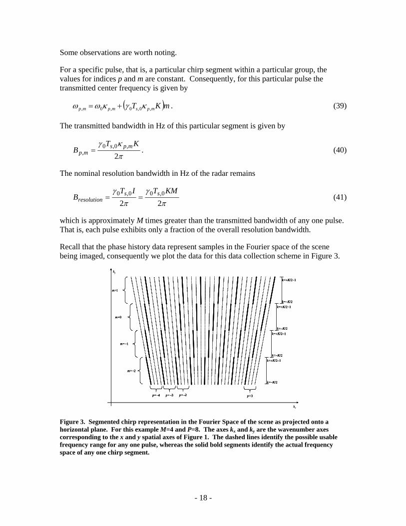
Recall that the phase history data represent samples in the Fourier space of the scene being imaged, consequently we plot the data for this data collection scheme in Figure 3.

m=−2

m=−1

m=0

m=1

p=−4 p=−3 p=−2 p=3

k=−K/2

k=+K/2−1

k=−K/2

k=+K/2−1

k=−K/2

k=+K/2−1

k=−K/2

k=+K/2−1

kx

ky

m=−2

m=−1

m=0

m=1

p=−4 p=−3 p=−2 p=3

k=−K/2

k=+K/2−1

k=−K/2

k=+K/2−1

k=−K/2

k=+K/2−1

k=−K/2

k=+K/2−1

m=−2

m=−1

m=0

m=1

p=−4 p=−3 p=−2 p=3

k=−K/2

k=+K/2−1

k=−K/2

k=+K/2−1

k=−K/2

k=+K/2−1

k=−K/2

k=+K/2−1

kx

ky

Figure 3. Segmented chirp representation in the Fourier Space of the scene as projected onto a horizontal plane. For this example M=4 and P=8. The axes kx and ky are the wavenumber axes corresponding to the x and y spatial axes of Figure 1. The dashed lines identify the possible usable frequency range for any one pulse, whereas the solid bold segments identify the actual frequency space of any one chirp segment.

- 18 -

Modified PFA Processing

Recall the model for the data

( ) ( )( ) ( )( )⎭⎬⎫

⎩⎨⎧ −+++= yxcsRV spMmdsmKkT

cjAmpkX αψγω 0,0,00 cos2exp,, . (42)

We write this now as

( )( )( ) ( )

( )( ) ⎪⎪⎭

⎪⎪⎬

⎫

⎪⎪⎩

⎪⎪⎨

⎧

++−

+++=

ycs

xcs

RV

smKkTc

pMmdsmKkTcjAmpkX

0,0,00

0,0,00

cos2

cos2

exp,,ψγω

αψγω. (43)

For a particular value of segment index m, data varies in azimuth with index p, and in range with index k. This data is on its own trapezoidal grid as shown in Figure 3, and can be processed accordingly.

Consistent with PFA processing, we require an azimuth resampling to a rectangular grid in the Fourier space projection. This is accomplished by interpolating the data such that

( ) ( ) npMmmKkTs ′=+⎟⎟

⎠

⎞⎜⎜⎝

⎛++

0

0,01ωγ

. (44)

The video signal data model thereby becomes

( )( )( ) ⎪

⎪⎭

⎪⎪⎬

⎫

⎪⎪⎩

⎪⎪⎨

⎧

++−

′=′

ycs

xc

RV

smKkTc

ndscjAmnkX

0,0,00

0,0

cos2

cos2

exp,,ψγω

αψω. (45)

At this point there is no reason to keep separate indices m and k anymore, and we can revert to the original fast-time index i. This yields

( )( ) ⎪

⎪⎭

⎪⎪⎬

⎫

⎪⎪⎩

⎪⎪⎨

⎧

+−

′=′

ycs

xc

RV

siTc

ndscjAniX

0,0,00

0,0

cos2

cos2

exp,ψγω

αψω (46)

which can be rewritten into the convenient and conventional form

- 19 -

( )

⎪⎪⎪

⎭

⎪⎪⎪

⎬

⎫

⎪⎪⎪

⎩

⎪⎪⎪

⎨

⎧

−

−

′

=′

yc

ycs

xc

RV

sc

isTc

ndsc

jAniX

0,0

0,0,0

0,0

cos2

cos2

cos2

exp,

ψω

ψγ

αψω

. (47)

This form has indices i and separated such that it exists on a rectangular grid, that is, it has been reformatted from the segmented trapezoidal grid of Figure 3 to a rectangular grid suitable for a conventional 2D DFT in the usual manner of image formation.

n′

Of course, the azimuth interpolation can be combined with the azimuth DFT in a variety of manners already reported in the literature.

Ramifications and Constraints

From Figure 3 we see that for any one frequency, only every Mth pulse contributes data. Consequently, to prevent aliasing, and all other things being equal, the minimum allowable Pulse Repetition Frequency (PRF) needs to increase by a factor of M from the non-segmented case.

Should pulse periods result that are less than echo delay time for the target scene of interest, then the minimum required PRF will cause “pulses in the air”.

From Figure 3 we also note that although N pulses are emitted, at any one frequency the data only spans pulses. This causes a very slight reduction in the achievable azimuth resolution. Of course this can be more than made up by collecting an additional

( )+− 1MN

M pulses.

- 20 -

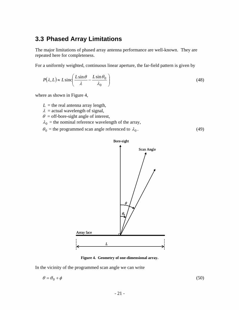
3.3 Phased Array Limitations The major limitations of phased array antenna performance are well-known. They are repeated here for completeness.

For a uniformly weighted, continuous linear aperture, the far-field pattern is given by

( ) ⎟⎟⎠

⎞⎜⎜⎝

⎛−≈

0

0sinsinsinc,λθ

λθλ

LLLLP (48)

where as shown in Figure 4,

L = the real antenna array length, λ = actual wavelength of signal, θ = off-bore-sight angle of interest,

0λ = the nominal reference wavelength of the array,

0θ = the programmed scan angle referenced to 0λ . (49)

L

Scan Angle

Bore-sight

Array face

θ

θ0

L

Scan Angle

Bore-sight

Array face

θ

θ0

Figure 4. Geometry of one-dimensional array.

In the vicinity of the programmed scan angle we can write

φθθ += 0 (50)

- 21 -

where φ is the deviation from the desired scan angle.

The peak response of the pattern is located when

( )0

00 sinsinλθ

λφθ

=+

. (51)

The nominal antenna beamwidth is approximately

0

0cosθλ

φLbeamwidth ≈ . (52)

The sensitivity of beam pointing to frequency or wavelength can be calculated as

000tan ff∂

−≈∂

≈∂

λλ

θφ (53)

where is the nominal center frequency in Hz. 0f

From this, the variation of pointing angle over signal bandwidth B is calculated as

00tan

fBθφ ≈∆ . (54)

Of course, we desire this to be much less than the beamwidth of the antenna, that is,

. beamwidthφφ <<∆ (55)

which becomes the constraint

0sinθLcB << . (56)

Interestingly, this is not dependent on wavelength, and can be further manipulated to the constraint on slant-range resolution as

2sin 0θρ

Lr >> . (57)

For these inequalities, one might presume that a factor of ten would suffice.

- 22 -

Radar PRF

We shall presume that the array is oriented with bore-sight oriented broadside to the radar flight path.

For broadside imaging, assuming the dimension L is the azimuth size of the array, the minimum radar PRF is calculated by Doerry23 as

Lvk

f xap

2≈ (58)

where

xv = the tangential velocity of the radar (forward velocity for the broadside case), and = the Doppler oversampling factor (typically on the order of 1.5 to 2.0). ak

(59)

In a squinted mode, the tangential velocity and the effective aperture size both reduce by a factor of cos 0θ , leaving the net relationship

Lvk

f xap

2≈ . (60)

As a side note, this suggests that an Exoclutter Ground Moving Target Indicator (GMTI) radar employing an AESA oriented to broadside derives no benefit to Minimum Detectable Velocity (MDV) by squinting forward or aft, as would a gimbaled antenna.

- 23 -

3.4 Parameter Selection For SAR operation, geometric parameters, including scan angle, are defined by the radar’s flight path and the target scene of interest.

Radar nominal frequency (or wavelength) are defined by the hardware of the system. Where choice is had, a frequency is chosen based on the phenomenology desired to be observed.

The phased-array antenna dimension is a function of the hardware as built.

Radar bandwidth is determined by the desired resolution with which the scene is to be rendered, by the well-known formula

rresolution

cBρ2

= . (61)

This ignores any sidelobe filtering effects.

Using a nominal factor of ten, the array usable bandwidth is calculated as

0sin101

θLcBarray ⎟

⎠⎞

⎜⎝⎛= . (62)

The number of chirp segments required then becomes bounded by their ratio, that is

array

resolutionB

BM ≥ . (63)

The minimum PRF is calculated to be

Lvk

Mf xap

2≈ . (64)

Design Example

Consider a Ku-band (16.8 GHz) SAR desiring to operate at a 45 degree scan angle with an AESA of width 0.3 m, and achieve 0.1 m resolution.

Using the above formulas, we calculate at this scan angle

resolutionB = 1.5 GHz, = 141 MHz, and arrayB

M = 11.

- 24 -

4 Conclusions The following principal conclusions should be drawn from this report.

• A phased array antenna steered by phase shifters alone has a finite bandwidth that depends on scan angle and array size.

• A chirp waveform can be divided into segments where the bandwidth of each segment is less than the limit imposed by the phased array antenna.

• Each chirp segment can be transmitted in a separate pulse. Doing so allows each pulse to be steered by phase shifters alone.

• The Phase History data can then be processed in a manner to reconstruct the image by combining all pulses with all chirp segments. In this manner the image will exhibit resolution consistent with the entire resolution bandwidth, which can be much larger than any segment’s chirp bandwidth.

- 25 -

“Fiction is obliged to stick to possibilities. Truth isn't.”

Mark Twain

- 26 -

REFERENCES

1 William J. Caputi, Jr., “Stretch: A Time-Transformation Technique”, IEEE Transactions on Aerospace and Electronic Systems, Vol. AES-7, No. 2, pp 269-278, March 1971.

2 J. L. Walker, “Range-Doppler Imaging of Rotating Objects,” IEEE Trans. on Aerospace and Electronic Systems, AES-16 (1), pp. 23-52, (1980).

3 M. Skolnik, Radar Handbook, second edition, ISBN 0-07-057913-X, McGraw-Hill, Inc., 1990.

4 G. Alberti, L . Citarella, L. Ciofaniello, R . Fusco, G. Galiero, A. Minoliti, A. Moccia, M. Sacchettino, G. Salzillo, “Current status about the development of an Italian airborne SAR system (MINISAR)”, Proceedings of the SPIE, Conference on SAR Image Analysis, Modeling and Techniques VI, Vol. 5236, pp 53-59, Barcelona, Spain, Sep. 08, 2003.

5 H. Schimpf, A. Wahlen, H. Essen, “High range resolution by means of synthetic bandwidth generated by frequency-stepped chirps”, IEE Electronics Letters, vol. 39, no. 18, pp 1346-8, 4 Sept. 2003.

6 T. Brehm, A.Wahlen, H. Essen, “High resolution millimeterwave SAR”, Conference Proceedings of the 1st European Radar Conference, pp 217-19, Amsterdam, Netherlands, 14-15 Oct. 2004.

7 Z. Yunhua, W. Jie, L. Haibin, “Two Simple and Efficient Approaches for Compressing Stepped Chirp Signals”, Proceedings of the 2005 Asia-Pacific Microwave Conference APMC2005, Vols 1-5, pp 690-693, Suzhou, China, 4-7 Dec. 2005.

8 R. Narayanan, P. C. Cantu, Xu Xiaojian, “An airborne low-cost SAR for remote sensing: hardware design and development”, Proceedings of IEEE International Geoscience and Remote Sensing Symposium IGARSS 2002, vol. 5, pp 2669-71, Toronto, Ont., Canada, 24-28 June 2002.

9 Michael T. Tuley, David M. Sheen, H. D. Collins, Earl V. Sager, and A. C. Schultheis, “Ultrawideband radar clutter measurements and analysis”, Proceedings of the SPIE, Conference on Ultrahigh Resolution Radar, Vol. 1875, pp. 124-133, Los Angeles, CA, USA, 20 January 1993.

- 27 -

10 M. Weiss, O. Saalmann, J. H. G. Ender, “A wideband phased array antenna for SAR application”, Conference Proceedings - 33rd European Microwave Conference, Vols 1-3, pp 511-514, Munich, Germany, Oct. 07-09, 2003.

11 D. R. Pape, A. P. Goutzoulis, “Wavelength Division Multiplexing Delay Broadcasting True-Time-Delay Network For Wideband Phased Array Antennas”, Proceedings of the SPIE, Optics in Computing 98 Meeting, Vol. 3490, pp 262-265., Brugge, Belgium, Jun 17-20, 1998.

12 R. Y. Loo, G. L. Tangonan, H. W. Yen, V. L. Jones, W. W. Ng, J. B. Lewis, “Photonics for Phased Array Antennas”, Proceedings of the SPIE, Conference on Photonics and Radio Frequency, vol. 2844, pp 234-240, Denver, CO, USA, 7-8 Aug. 1996.

13 A. P. Goutzoulis, D. K. Davies, J. M. Zomp, “Hybrid electronic fiber optic wavelength-multiplexed system for true time-delay steering of phased array antennas”, Optical Engineering, Vol. 31, No. 11, pp 2312-2322, November 1992.

14 M. A. Fischman, C. Le, P. A. Rosen, “A digital beamforming processor for the joint DoD/NASA space based radar mission”, Proceedings of the 2004 IEEE Radar Conference, pp 9-14, Philadelphia, PA, USA, 26-29 April 2004.

15 Jack J. Schuss, Jerome D. Hanfling, “Space fed antenna system with squint error correction”, US Patent 4,743,914, May 10, 1988.

16 Eric N. Boe, Robert E. Shuman, Richard D. Young, Hoyoung C. Choe, Adam C. Von, “Digital beam stabilization techniques for wide-bandwidth electronically scanned antennas”, US Patent 6,693,589, February 17, 2004.

17 M. I. Skolnik, Introduction to Radar Systems, second edition, ISBN 0-07-057909-1, McGraw-Hill, Inc., 1980.

18 Walter G. Carrara, Ron S. Goodman, Ronald M. Majewski, Spotlight Synthetic Aperture Radar, Signal Processing Algorithms, ISBN 0-89006-728-7, Artech House Publishers, 1995.

19 C. V. Jakowatz Jr., D. E. Wahl, P. H. Eichel, D. C. Ghiglia, P. A. Thompson, Spotlight-Mode Synthetic Aperture Radar: A Signal Processing Approach, ISBN 0-7923-9677-4, Kluwer Academic Publishers, 1996.

20 Grant D. Martin, Armin W. Doerry, Michael W. Holzrichter, “A Novel Polar Format Algorithm for SAR Images Utilizing Post Azimuth Transform Interpolation”, Sandia Report SAND2005-5510, Unlimited Release, September 2005.

- 28 -

21 Grant D. Martin, Armin W. Doerry, “SAR Polar Format Implementation with MATLAB”, Sandia Report SAND2005-7413, Unlimited Release, November 2005.

22 Doerry, Armin W., “Real-time Polar-Format Processing for Sandia’s Testbed Radar Systems”, Sandia Internal Memorandum SAND2001-1644P, Internal Distribution Only, June 2001.

23 A. W. Doerry, “Performance Limits for Synthetic Aperture Radar – second edition”, Sandia Report SAND2006-0821, Unlimited Release, February 2006.

- 29 -

DISTRIBUTION Unlimited Release

1 MS 1330 B. L. Remund 5340 1 MS 1330 B. L. Burns 5340

1 MS 1330 W. H. Hensley 5342 1 MS 1330 T. P. Bielek 5342 1 MS 1330 A. W. Doerry 5342 1 MS 1330 S. S. Kawka 5342 1 MS 1330 D. G. Thompson 5342 1 MS 1330 K. W. Sorensen 5345 1 MS 1330 S. E. Allen 5345 1 MS 0529 K. C. Branch 5345 1 MS 0529 B. C. Brock 5345 1 MS 1330 D. F. Dubbert 5345 1 MS 1330 G. R. Sloan 5345 1 MS 1330 B. H. Strassner 5345 1 MS 1330 S. M. Becker 5348 1 MS 1330 M. W. Holzrichter 5348 1 MS 1330 D. C. Sprauer 5348 1 MS 1330 A. D. Sweet 5348 1 MS 1330 O. M. Jeromin 5348 1 MS 0519 D. L. Bickel 5354 1 MS 0519 J. T. Cordaro 5354 1 MS 0519 J. DeLaurentis 5354 2 MS 9018 Central Technical Files 8944 2 MS 0899 Technical Library 4536

- 30 -