Operations Research Letters 38 (2010) 51–56

Contents lists available at ScienceDirect

Operations Research Letters

journal homepage: www.elsevier.com/locate/orl

Scheduling Markovian PERT networks to maximize the net present valueStefan Creemers a, Roel Leus b,∗, Marc Lambrecht aa Research Center for Operations Management, Faculty of Business and Economics, Katholieke Universiteit Leuven, Belgiumb Research Center for Operations Research & Business Statistics (ORSTAT), Faculty of Business and Economics, Katholieke Universiteit Leuven, Belgium

a r t i c l e i n f o

Article history:Received 9 May 2008Accepted 7 October 2009Available online 24 October 2009

Keywords:Project schedulingNet present valueStochastic activity durationsExponential distribution

a b s t r a c t

Weexamine project schedulingwith net present value objective and exponential activity durations, usinga continuous-time Markov decision chain. On the basis of a judicious partitioning of the state space, weachieve a significant performance improvement as compared to the existing algorithms.

© 2009 Elsevier B.V. All rights reserved.

1. Introduction

A project consists of a set of activities (or tasks) N = 0, 1,. . . , n, which are to be processed without interruption. The du-ration Di of each activity i is a random variable; the vector(D0,D1, . . . ,Dn) is denoted by D. The set A is a strict order on N ,i.e. an irreflexive and transitive relation, which represents tech-nological precedence constraints. The activities 0 and n representthe start and end of the project, respectively, and are the (unique)smallest and largest elements of the partially ordered set (N, A).We use lower-case vector d = (d0, d1, . . . , dn) to represent oneparticular realization (or sample, or scenario) of D. Alternatively,when each duration Di is a constant, we use the same notation d.For a given realization d, we can produce a schedule s, i.e., a vec-tor of starting times (s0, s1, . . . , sn) with si ≥ 0 for all i ∈ N . Theschedule s is feasible if si + di ≤ sj for all (i, j) ∈ A.In the absence of resource constraints, theminimum-makespan

objective requires no real scheduling effort: all activities arestarted as soon as their predecessors are completed. The literatureon this so-called PERT problem is usually concerned withthe computation of certain characteristics of the minimumproject makespan (earliest project completion) when the activitydurations are random variables, mainly with exact computation,approximation and bounding of the distribution function andthe expected value [1,4,7]. A Markovian PERT network is a PERTnetwork with independent and exponentially distributed activity

∗ Corresponding address: Department of Decision Sciences and InformationManagement, Katholieke Universiteit Leuven, Naamsestraat 69, 3000 Leuven,Belgium. Tel.: +32 16 32 69 67; fax: +32 16 32 66 24.E-mail address: Roel.Leus@econ.kuleuven.be (R. Leus).

0167-6377/$ – see front matter© 2009 Elsevier B.V. All rights reserved.doi:10.1016/j.orl.2009.10.006

durations. For such Markovian PERT networks, Kulkarni andAdlakha [6] describe an exact method for deriving the distributionand moments of the earliest project completion time usingContinuous-Time Markov Chains (CTMCs).In this article, we focus on project scheduling with NPV (net

present value) objective and exponential durations [2,9]. Eachactivity i ∈ N generates a cash flow ci, which is a rational numberthat may be positive or negative; this quantity is received or paidat the start of the activity. In order to account for the time valueof money, we define r to be the applicable continuous discountrate: the present value of a cash flow c incurred at time t equalsce−rt . Both Sobel et al. [9] and Buss and Rosenblatt [2] use theCTMC described in [6] as a starting point for their algorithm.Buss and Rosenblatt always start all eligible activities as soon aspossible (but after a delay period, which is individually chosenfor each activity), and so they make no further decisions once theproject is in progress. We study the same problem as Sobel et al.,in which activities are only started at the end of other activities(see the next section for a detailed problem statement). On thebasis of a judicious partitioning of the state space, we achieve asignificant performance improvement compared to Sobel et al.,both on running times as well as on memory usage.

2. Problem statement

The execution of a project with stochastic durations can best beseen as a dynamic decision process. A solution is a policyΠ , whichdefines actions at decision times. Decision times are typically t = 0(the start of the project) and the completion times of activities; atentative next decision time can also be specified by the decisionmaker. An action can entail the start of a set of activities that is‘feasible’, meaning that a feasible schedule is constructed gradually

52 S. Creemers et al. / Operations Research Letters 38 (2010) 51–56

through time. Besides the input data of the problem instance, adecision at time t can only use information (on activity-durationrealizations) that has become available before or at time t; thisrequirement is often referred to as the non-anticipativity constraint.As soon as all activities are completed, the activity durations are

known, yielding a realization d of D. Consequently, every policyΠmay alternatively be interpreted [5] as a function Rn+1

≥7→ Rn+1

≥

that maps given samples d of activity durations to vectors s(d;Π)of feasible activity starting times (schedules). For a given scenariod and policy Π , sn(d;Π) denotes the makespan of the schedule.The earlier-mentioned PERT problem aims at characterizing therandom variable sn(D;ΠES), where policy ΠES starts all activitiesas early as possible. Contrary to e.g. the expected makespan,however, NPV is a non-regular measure of performance: startingactivities as early as possible is not necessarily optimal, since the cimay be negative.We investigate the determination of an optimal scheduling

policy for the expected-NPV objective. In the special case wherethe durations have constant values d, the objective functioncorresponding with a schedule s is the following:

max g(s, d) =n∑i=0

cie−rsi

subject to

si + di ≤ sj ∀(i, j) ∈ A.

Our goal is to select a policy Π∗ within a specific class thatmaximizes E[g(s(D;Π),D)], with E[·] the expectation operatorwith respect to D. The generality of this problem statementsuggests that optimization over the class of all policies willprobably turn out to be computationally intractable. We thereforerestrict our attention to a subclass that has a simple combinatorialrepresentation and where decision points are limited in number:our solution space consists of all policies that start activities onlyat the end of other activities (activity 0 is started at time 0).

3. The algorithm

We assume the durations of the activities i ∈ N \ 0, n to bemutually independent exponentially distributed random variableswith mean 1

µi, µi > 0. Section 3.1 briefly presents the state space

of our search procedure, Section 3.2 discusses how we partitionthis state space in order to facilitatememorymanagement, and thestochastic dynamic-programming (SDP) algorithm that producesan optimal policy is the subject of Section 3.3.

3.1. State space

At any time instant t , each activity’s status is either idle (= un-started), active (= in the process of being executed) or finished; wewrite Ωi(t) = 0, 1 or 2, respectively, for i ∈ N . The state of thesystem is defined by the status of the individual activities and isrepresented by vector Ω(t) = (Ω0(t),Ω1(t), . . . ,Ωn(t)). Statetransitions take place each time an activity finishes and are deter-mined by the policy at hand. The project’s starting and finishingconditions are ∀i ∈ N : Ωi(0) = 0 and ∀i ∈ N : Ωi(t) = 2, ∀t ≥ ω,respectively, where ω indicates the project completion time. Theproblemof finding an optimal scheduling policy corresponds to op-timizing a discounted criterion in a Continuous-TimeMarkovDeci-sion Chain (CTMDC) on the state space Q , with Q containing all thestates of the system that canbe visited by the transitions (which arecalled feasible states); the decision set is described in Section 3.3.An upper bound on |Q | is 3n. Enumerating all these 3n states

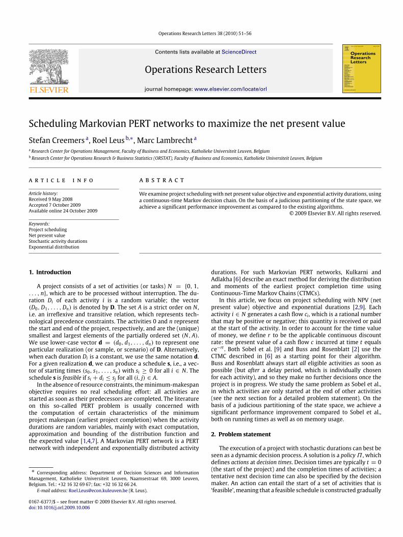
is not recommended, because typically the majority of the statesdo not satisfy the precedence constraints. Sobel et al. [9] develop

Fig. 1. Example project network.

a simple yet efficient algorithm for producing a set of possiblestates; this set contains Q but may be strictly larger. Additionally,to the best of our knowledge, all related studies in the literaturereserve memory space for storing the entire state space of theCTMDC; Buss and Rosenblatt [2] point out that some method ofdecomposition for reducing these memory requirements wouldallow for considerable efficiency enhancements. In what follows,we present an algorithm that considerably improves upon thestorage and computational requirements of earlier algorithms bymeans of efficient creation of Q and decomposition of the networkof state transitions.

3.2. Uniformly directed cuts

Our algorithm consists of two main steps. This subsectiondiscusses the first step, which is the generation of all inclusion-maximal antichains of A (sets of activities that can be executed inparallel). Kulkarni and Adlakha [6] refer to these sets as uniformlydirected cuts or UDCs, and we will retain this term (althoughwe work with activity-on-the-node instead of activity-on-the-arcrepresentation). In the second step of the algorithm, we applya backward SDP recursion to determine optimal decisions; thisrecursion is the subject of Section 3.3.Let U =

U1,U2, . . . ,U|U|

denote the set of UDCs. Formally,

U is themaximum-size subset of the power set 2N whose elementsU satisfy the following conditions:

(1) ∀i, j ⊂ U : (i, j) 6∈ A ∧ (j, i) 6∈ A,(2) @u ∈ N \ U : U ∪ u satisfies condition (1).

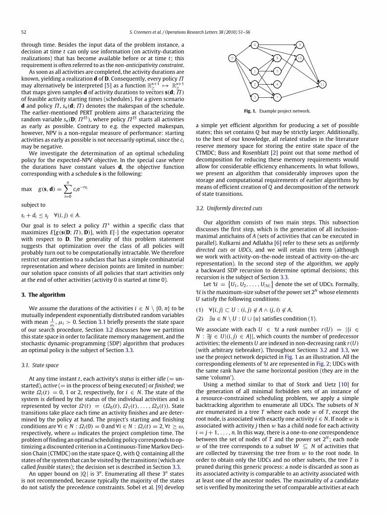
We associate with each U ∈ U a rank number r(U) = |i ∈N : ∃j ∈ U|(i, j) ∈ A|, which counts the number of predecessoractivities; the elementsU are indexed in non-decreasing rank r(U)(with arbitrary tiebreaker). Throughout Sections 3.2 and 3.3, weuse the project network depicted in Fig. 1 as an illustration. All thecorresponding elements ofU are represented in Fig. 2; UDCs withthe same rank have the same horizontal position (they are in thesame ‘column’).Using a method similar to that of Stork and Uetz [10] for

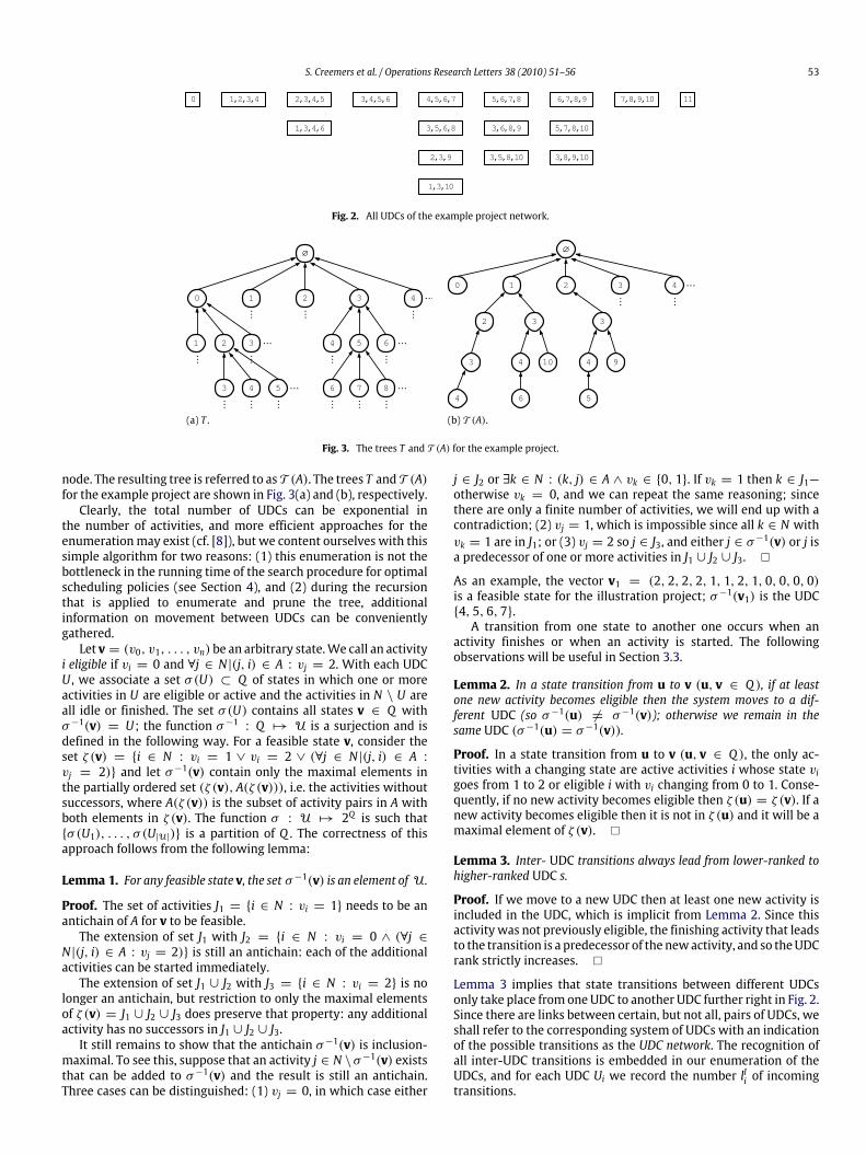
the generation of all minimal forbidden sets of an instance ofa resource-constrained scheduling problem, we apply a simplebacktracking algorithm to enumerate all UDCs. The subsets of Nare enumerated in a tree T where each node w of T , except theroot node, is associated with exactly one activity i ∈ N . If nodew isassociated with activity j then w has a child node for each activityi = j+ 1, . . . , n. In this way, there is a one-to-one correspondencebetween the set of nodes of T and the power set 2N ; each nodew of the tree corresponds to a subset W ⊆ N of activities thatare collected by traversing the tree from w to the root node. Inorder to obtain only the UDCs and no other subsets, the tree T ispruned during this generic process: a node is discarded as soon asits associated activity is comparable to an activity associated withat least one of the ancestor nodes. The maximality of a candidateset is verified bymonitoring the set of comparable activities at each

S. Creemers et al. / Operations Research Letters 38 (2010) 51–56 53

Fig. 2. All UDCs of the example project network.

(a) T . (b) T (A).

Fig. 3. The trees T and T (A) for the example project.

node. The resulting tree is referred to as T (A). The trees T and T (A)for the example project are shown in Fig. 3(a) and (b), respectively.Clearly, the total number of UDCs can be exponential in

the number of activities, and more efficient approaches for theenumerationmay exist (cf. [8]), but we content ourselves with thissimple algorithm for two reasons: (1) this enumeration is not thebottleneck in the running time of the search procedure for optimalscheduling policies (see Section 4), and (2) during the recursionthat is applied to enumerate and prune the tree, additionalinformation on movement between UDCs can be convenientlygathered.Let v = (v0, v1, . . . , vn) be an arbitrary state.We call an activity

i eligible if vi = 0 and ∀j ∈ N|(j, i) ∈ A : vj = 2. With each UDCU , we associate a set σ(U) ⊂ Q of states in which one or moreactivities in U are eligible or active and the activities in N \ U areall idle or finished. The set σ(U) contains all states v ∈ Q withσ−1(v) = U; the function σ−1 : Q 7→ U is a surjection and isdefined in the following way. For a feasible state v, consider theset ζ (v) = i ∈ N : vi = 1 ∨ vi = 2 ∨ (∀j ∈ N|(j, i) ∈ A :vj = 2) and let σ−1(v) contain only the maximal elements inthe partially ordered set (ζ (v), A(ζ (v))), i.e. the activities withoutsuccessors, where A(ζ (v)) is the subset of activity pairs in A withboth elements in ζ (v). The function σ : U 7→ 2Q is such thatσ(U1), . . . , σ (U|U|) is a partition of Q . The correctness of thisapproach follows from the following lemma:

Lemma 1. For any feasible state v, the set σ−1(v) is an element of U.

Proof. The set of activities J1 = i ∈ N : vi = 1 needs to be anantichain of A for v to be feasible.The extension of set J1 with J2 = i ∈ N : vi = 0 ∧ (∀j ∈

N|(j, i) ∈ A : vj = 2) is still an antichain: each of the additionalactivities can be started immediately.The extension of set J1 ∪ J2 with J3 = i ∈ N : vi = 2 is no

longer an antichain, but restriction to only the maximal elementsof ζ (v) = J1 ∪ J2 ∪ J3 does preserve that property: any additionalactivity has no successors in J1 ∪ J2 ∪ J3.It still remains to show that the antichain σ−1(v) is inclusion-

maximal. To see this, suppose that an activity j ∈ N \σ−1(v) existsthat can be added to σ−1(v) and the result is still an antichain.Three cases can be distinguished: (1) vj = 0, in which case either

j ∈ J2 or ∃k ∈ N : (k, j) ∈ A ∧ vk ∈ 0, 1. If vk = 1 then k ∈ J1—otherwise vk = 0, and we can repeat the same reasoning; sincethere are only a finite number of activities, we will end up with acontradiction; (2) vj = 1, which is impossible since all k ∈ N withvk = 1 are in J1; or (3) vj = 2 so j ∈ J3, and either j ∈ σ−1(v) or j isa predecessor of one or more activities in J1 ∪ J2 ∪ J3.

As an example, the vector v1 = (2, 2, 2, 2, 1, 1, 2, 1, 0, 0, 0, 0)is a feasible state for the illustration project; σ−1(v1) is the UDC4, 5, 6, 7.A transition from one state to another one occurs when an

activity finishes or when an activity is started. The followingobservations will be useful in Section 3.3.

Lemma 2. In a state transition from u to v (u, v ∈ Q ), if at leastone new activity becomes eligible then the system moves to a dif-ferent UDC (so σ−1(u) 6= σ−1(v)); otherwise we remain in thesame UDC (σ−1(u) = σ−1(v)).

Proof. In a state transition from u to v (u, v ∈ Q ), the only ac-tivities with a changing state are active activities i whose state vigoes from 1 to 2 or eligible i with vi changing from 0 to 1. Conse-quently, if no new activity becomes eligible then ζ (u) = ζ (v). If anew activity becomes eligible then it is not in ζ (u) and it will be amaximal element of ζ (v).

Lemma 3. Inter- UDC transitions always lead from lower-ranked tohigher-ranked UDC s.

Proof. If we move to a new UDC then at least one new activity isincluded in the UDC, which is implicit from Lemma 2. Since thisactivity was not previously eligible, the finishing activity that leadsto the transition is a predecessor of the newactivity, and so theUDCrank strictly increases.

Lemma 3 implies that state transitions between different UDCsonly take place from one UDC to another UDC further right in Fig. 2.Since there are links between certain, but not all, pairs of UDCs, weshall refer to the corresponding system of UDCs with an indicationof the possible transitions as the UDC network. The recognition ofall inter-UDC transitions is embedded in our enumeration of theUDCs, and for each UDC Ui we record the number lIi of incomingtransitions.

54 S. Creemers et al. / Operations Research Letters 38 (2010) 51–56

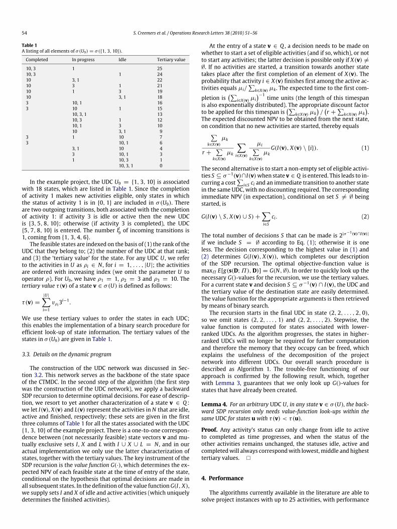
Table 1A listing of all elements of σ(U9) = σ(1, 3, 10).

Completed In progress Idle Tertiary value

10, 3 1 2510, 3 1 2410 3, 1 2210 3 1 2110 1 3 1910 3, 1 183 10, 1 163 10 1 15

10, 3, 1 1310, 3 1 1210, 1 3 1010 3, 1 9

3 1 10 73 10, 1 6

3, 1 10 43 10, 1 31 10, 3 1

10, 3, 1 0

In the example project, the UDC U9 = 1, 3, 10 is associatedwith 18 states, which are listed in Table 1. Since the completionof activity 1 makes new activities eligible, only states in whichthe status of activity 1 is in 0, 1 are included in σ(U9). Thereare two outgoing transitions, both associated with the completionof activity 1: if activity 3 is idle or active then the new UDCis 3, 5, 8, 10; otherwise (if activity 3 is completed), the UDC5, 7, 8, 10 is entered. The number lI9 of incoming transitions is1, coming from 1, 3, 4, 6.The feasible states are indexed on the basis of (1) the rank of the

UDC that they belong to; (2) the number of the UDC at that rank;and (3) the ‘tertiary value’ for the state. For any UDC U , we referto the activities in U as ρi ∈ N , for i = 1, . . . , |U|; the activitiesare ordered with increasing index (we omit the parameter U tooperator ρ). For U9, we have ρ1 = 1, ρ2 = 3 and ρ3 = 10. Thetertiary value τ(v) of a state v ∈ σ(U) is defined as follows:

τ(v) =|U|∑i=1

vρi3i−1.

We use these tertiary values to order the states in each UDC;this enables the implementation of a binary search procedure forefficient look-up of state information. The tertiary values of thestates in σ(U9) are given in Table 1.

3.3. Details on the dynamic program

The construction of the UDC network was discussed in Sec-tion 3.2. This network serves as the backbone of the state spaceof the CTMDC. In the second step of the algorithm (the first stepwas the construction of the UDC network), we apply a backwardSDP recursion to determine optimal decisions. For ease of descrip-tion, we resort to yet another characterization of a state v ∈ Q :we let I(v), X(v) and L(v) represent the activities in N that are idle,active and finished, respectively; these sets are given in the firstthree columns of Table 1 for all the states associated with the UDC1, 3, 10 of the example project. There is a one-to-one correspon-dence between (not necessarily feasible) state vectors v and mu-tually exclusive sets I , X and L with I ∪ X ∪ L = N , and in ouractual implementation we only use the latter characterization ofstates, together with the tertiary values. The key instrument of theSDP recursion is the value function G(·), which determines the ex-pected NPV of each feasible state at the time of entry of the state,conditional on the hypothesis that optimal decisions are made inall subsequent states. In the definition of the value functionG(I, X),we supply sets I and X of idle and active activities (which uniquelydetermines the finished activities).

At the entry of a state v ∈ Q , a decision needs to be made onwhether to start a set of eligible activities (and if so, which), or notto start any activities; the latter decision is possible only if X(v) 6=∅. If no activities are started, a transition towards another statetakes place after the first completion of an element of X(v). Theprobability that activity i ∈ X(v) finishes first among the active ac-tivities equals µi/

∑k∈X(v) µk. The expected time to the first com-

pletion is(∑

i∈X(v) µi)−1 time units (the length of this timespan

is also exponentially distributed). The appropriate discount factorto be applied for this timespan is

(∑k∈X(v) µk

)/(r +

∑k∈X(v) µk

).

The expected discounted NPV to be obtained from the next state,on condition that no new activities are started, thereby equals∑k∈X(v)

µk

r +∑k∈X(v)

µk

∑i∈X(v)

µi∑k∈X(v)

µkG(I(v), X(v) \ i). (1)

The second alternative is to start a non-empty set of eligible activi-ties S ⊆ σ−1(v)∩I(v)when state v ∈ Q is entered. This leads to in-curring a cost

∑i∈S ci and an immediate transition to another state

in the same UDC, with no discounting required. The correspondingimmediate NPV (in expectation), conditional on set S 6= ∅ beingstarted, is

G(I(v) \ S, X(v) ∪ S)+∑i∈S

ci. (2)

The total number of decisions S that can be made is 2|σ−1(v)∩I(v)|

if we include S = ∅ according to Eq. (1); otherwise it is oneless. The decision corresponding to the highest value in (1) and(2) determines G(I(v), X(v)), which completes our descriptionof the SDP recursion. The optimal objective-function value ismaxΠ E[g(s(D;Π),D)] = G(N,∅). In order to quickly look up thenecessary G()-values for the recursion, we use the tertiary values.For a current state v and decision S ⊆ σ−1(v) ∩ I(v), the UDC andthe tertiary value of the destination state are easily determined.The value function for the appropriate arguments is then retrievedby means of binary search.The recursion starts in the final UDC in state (2, 2, . . . , 2, 0),

so we omit states (2, 2, . . . , 1) and (2, 2, . . . , 2). Stepwise, thevalue function is computed for states associated with lower-ranked UDCs. As the algorithm progresses, the states in higher-ranked UDCs will no longer be required for further computationand therefore the memory that they occupy can be freed, whichexplains the usefulness of the decomposition of the projectnetwork into different UDCs. Our overall search procedure isdescribed as Algorithm 1. The trouble-free functioning of ourapproach is confirmed by the following result, which, togetherwith Lemma 3, guarantees that we only look up G()-values forstates that have already been created.

Lemma 4. For an arbitrary UDC U, in any state v ∈ σ(U), the back-ward SDP recursion only needs value-function look-ups within thesame UDC for states u with τ(v) < τ(u).

Proof. Any activity’s status can only change from idle to activeto completed as time progresses, and when the status of theother activities remains unchanged, the statuses idle, active andcompletedwill always correspondwith lowest,middle and highesttertiary values.

4. Performance

The algorithms currently available in the literature are able tosolve project instances with up to 25 activities, with performance

S. Creemers et al. / Operations Research Letters 38 (2010) 51–56 55

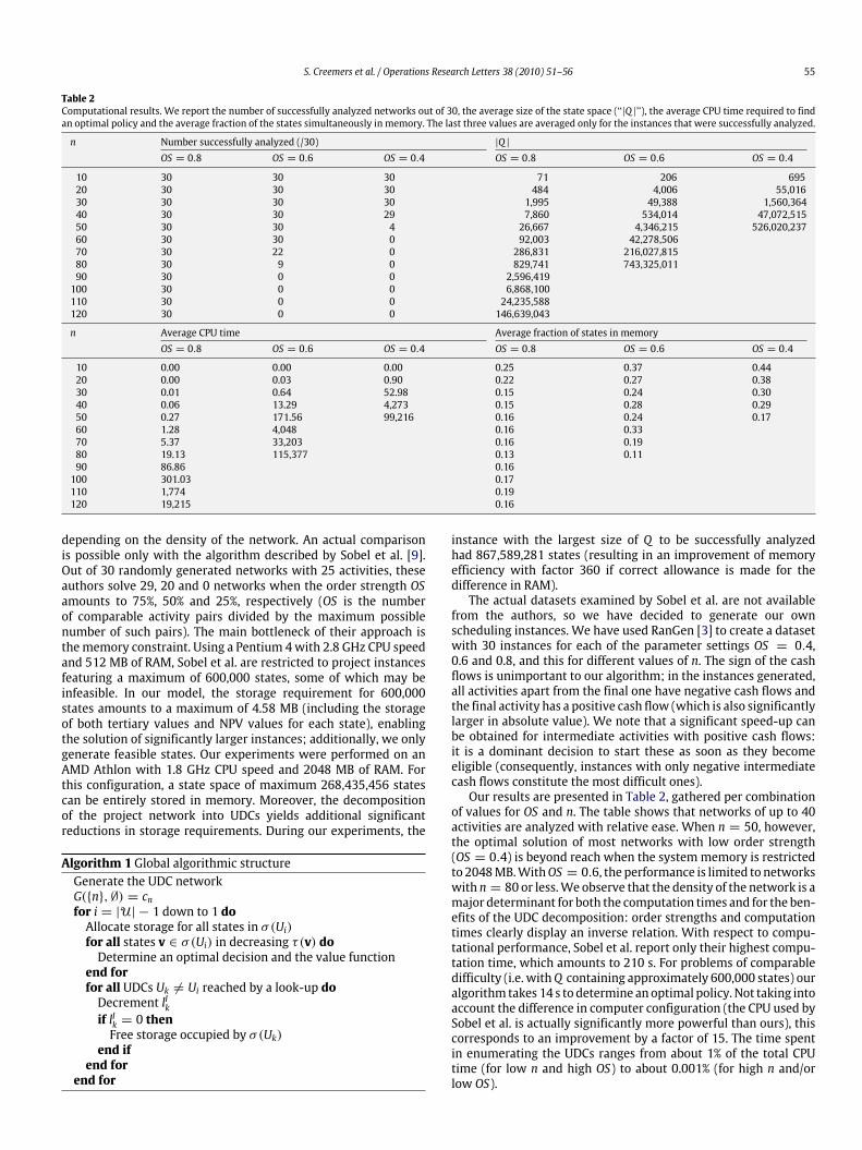
Table 2Computational results. We report the number of successfully analyzed networks out of 30, the average size of the state space (‘‘|Q |’’), the average CPU time required to findan optimal policy and the average fraction of the states simultaneously in memory. The last three values are averaged only for the instances that were successfully analyzed.

n Number successfully analyzed (/30) |Q |OS = 0.8 OS = 0.6 OS = 0.4 OS = 0.8 OS = 0.6 OS = 0.4

10 30 30 30 71 206 69520 30 30 30 484 4,006 55,01630 30 30 30 1,995 49,388 1,560,36440 30 30 29 7,860 534,014 47,072,51550 30 30 4 26,667 4,346,215 526,020,23760 30 30 0 92,003 42,278,50670 30 22 0 286,831 216,027,81580 30 9 0 829,741 743,325,01190 30 0 0 2,596,419100 30 0 0 6,868,100110 30 0 0 24,235,588120 30 0 0 146,639,043

n Average CPU time Average fraction of states in memoryOS = 0.8 OS = 0.6 OS = 0.4 OS = 0.8 OS = 0.6 OS = 0.4

10 0.00 0.00 0.00 0.25 0.37 0.4420 0.00 0.03 0.90 0.22 0.27 0.3830 0.01 0.64 52.98 0.15 0.24 0.3040 0.06 13.29 4,273 0.15 0.28 0.2950 0.27 171.56 99,216 0.16 0.24 0.1760 1.28 4,048 0.16 0.3370 5.37 33,203 0.16 0.1980 19.13 115,377 0.13 0.1190 86.86 0.16100 301.03 0.17110 1,774 0.19120 19,215 0.16

depending on the density of the network. An actual comparisonis possible only with the algorithm described by Sobel et al. [9].Out of 30 randomly generated networks with 25 activities, theseauthors solve 29, 20 and 0 networks when the order strength OSamounts to 75%, 50% and 25%, respectively (OS is the numberof comparable activity pairs divided by the maximum possiblenumber of such pairs). The main bottleneck of their approach isthememory constraint. Using a Pentium 4with 2.8 GHz CPU speedand 512 MB of RAM, Sobel et al. are restricted to project instancesfeaturing a maximum of 600,000 states, some of which may beinfeasible. In our model, the storage requirement for 600,000states amounts to a maximum of 4.58 MB (including the storageof both tertiary values and NPV values for each state), enablingthe solution of significantly larger instances; additionally, we onlygenerate feasible states. Our experiments were performed on anAMD Athlon with 1.8 GHz CPU speed and 2048 MB of RAM. Forthis configuration, a state space of maximum 268,435,456 statescan be entirely stored in memory. Moreover, the decompositionof the project network into UDCs yields additional significantreductions in storage requirements. During our experiments, the

Algorithm 1 Global algorithmic structureGenerate the UDC networkG(n,∅) = cnfor i = |U| − 1 down to 1 doAllocate storage for all states in σ(Ui)for all states v ∈ σ(Ui) in decreasing τ(v) doDetermine an optimal decision and the value function

end forfor all UDCs Uk 6= Ui reached by a look-up doDecrement lIkif lIk = 0 thenFree storage occupied by σ(Uk)

end ifend for

end for

instance with the largest size of Q to be successfully analyzedhad 867,589,281 states (resulting in an improvement of memoryefficiency with factor 360 if correct allowance is made for thedifference in RAM).The actual datasets examined by Sobel et al. are not available

from the authors, so we have decided to generate our ownscheduling instances. We have used RanGen [3] to create a datasetwith 30 instances for each of the parameter settings OS = 0.4,0.6 and 0.8, and this for different values of n. The sign of the cashflows is unimportant to our algorithm; in the instances generated,all activities apart from the final one have negative cash flows andthe final activity has a positive cash flow (which is also significantlylarger in absolute value). We note that a significant speed-up canbe obtained for intermediate activities with positive cash flows:it is a dominant decision to start these as soon as they becomeeligible (consequently, instances with only negative intermediatecash flows constitute the most difficult ones).Our results are presented in Table 2, gathered per combination

of values for OS and n. The table shows that networks of up to 40activities are analyzed with relative ease. When n = 50, however,the optimal solution of most networks with low order strength(OS = 0.4) is beyond reach when the systemmemory is restrictedto 2048MB.WithOS = 0.6, the performance is limited to networkswith n = 80 or less.We observe that the density of the network is amajor determinant for both the computation times and for the ben-efits of the UDC decomposition: order strengths and computationtimes clearly display an inverse relation. With respect to compu-tational performance, Sobel et al. report only their highest compu-tation time, which amounts to 210 s. For problems of comparabledifficulty (i.e. withQ containing approximately 600,000 states) ouralgorithm takes 14 s to determine anoptimal policy. Not taking intoaccount the difference in computer configuration (the CPU used bySobel et al. is actually significantly more powerful than ours), thiscorresponds to an improvement by a factor of 15. The time spentin enumerating the UDCs ranges from about 1% of the total CPUtime (for low n and high OS) to about 0.001% (for high n and/orlow OS).

56 S. Creemers et al. / Operations Research Letters 38 (2010) 51–56

Acknowledgement

We are grateful to Prof. Bert De Reyck for some insightful sug-gestions. This work was supported by research projects G.0578.07and G.0547.09 of the Research Foundation – Flanders (FWO) (Bel-gium).

References

[1] V.G. Adlakha, V.G. Kulkarni, A classified bibliography of research on stochasticPERT networks: 1966–1987, INFOR 27 (1989) 272–296.

[2] A.H. Buss, Rosenblatt. Activity delay in stochastic project networks, OperationsResearch 45 (1997) 126–139.

[3] E. Demeulemeester, M. Vanhoucke, W. Herroelen, A random network genera-tor for activity-on-the-node networks, Journal of Scheduling 6 (2003) 13–34.

[4] S.E. Elmaghraby, Activity Networks: Project Planning and Control by NetworkModels, Wiley, 1977.

[5] G. Igelmund, F.J. Radermacher, Preselective strategies for the optimization ofstochastic project networks under resource constraints, Networks 13 (1983)1–28.

[6] V.G. Kulkarni, V.G. Adlakha, Markov andMarkov-regenerative PERT networks,Operations Research 34 (1986) 769–781.

[7] A. Ludwig, R.H. Möhring, F. Stork, A computational study on bounding themakespan distribution in stochastic project networks, Annals of OperationsResearch 102 (2001) 49–64.

[8] D.R. Shier, D.E. Whited, Iterative algorithms for generating minimal cutsets indirected graphs, Networks 16 (1986) 133–147.

[9] M.J. Sobel, J.G. Szmerekovsky, V. Tilson, Scheduling projects with stochasticactivity duration to maximize expected net present value, European Journalof Operational Research 198 (2009) 697–705.

[10] F. Stork, M. Uetz, On the generation of circuits and minimal forbidden sets,Mathematical Programming 102 (2005) 185–203.