Scheduling parallel machines with a single server: some solvable cases and heuristics

Computers & Operations Research 29 (2002) 295}315

Scheduling parallel machines with a single server:some solvable cases and heuristics

Amir H. Abdekhodaee, Andrew Wirth*

Department of Mechanical and Manufacturing Engineering, The University of Melbourne, Vic 3010, Australia

Received 1 October 1998; received in revised form 1 April 1999

Abstract

This paper considers the problem of scheduling two identical parallel machines with a single server whichis required to carry out the job setups. Job processing can then be carried out in parallel. The objective is tominimise maximum completion time, that is makespan. The problem is NP-complete in the strong sense.An integer program formulation is presented. Two special cases: short processing times and equal length jobsare solved. Two simple but e!ective O(n log n) heuristics for the general case are given and their performanceis tested.

Scope and purpose

A common problem in manufacturing is the need to share a common server, for example a robot, bya number of machines to carry out machine setups. Job processing is then executed automatically andindependently by the individual machines. Sharing the server resource results in machine idle time. Theobjective is to "nd the schedule which minimises the makespan. This paper solves exactly the special case ofequal length jobs and provides e$cient and e!ective heuristics for the general problem. � 2001 ElsevierScience Ltd. All rights reserved.

Keywords: Scheduling; Parallel machines; Server

1. Introduction

Problems dealing with parallel machines for which each job requires a setup to be carried out,immediately prior to its processing, by a single server, with the processing executed unattended,

* Corresponding author. Tel.: #61-3-8344-4852; fax: #61-3-9347-8784.E-mail address: [email protected] (A. Wirth).

0305-0548/01/$ - see front matter � 2001 Elsevier Science Ltd. All rights reserved.PII: S 0 3 0 5 - 0 5 4 8 ( 0 0 ) 0 0 0 7 4 - 5

have received scant attention in the literature. In fact, we are aware of only four papers onthe subject, Koulamas and Smith [1], Hall et al. [2], Koulamas [3] and Kravchenko and Werner[4] most of which have been published recently and include some complementary results. Thesepapers mainly discuss the complexity of the makespan minimisation problem and its counterpartmachine interference time (the time machines are idle due to unavailability of the server, ona machine after all of its processing is completed, is ignored). They provide no computationalanalysis for the makespan problem nor do they discuss the exact solution of the special caseconsidered below.

The above issue was motivated by a problem in the manufacture of automobile components.Bourland and Carl [5] reported work on a similar problem, however they assumed that more thanone machine may be served at the one time, the fractional operator problem. The literature onresource constrained scheduling, for example that found in Blazewicz et al. [6] or Lawler et al. [7]assumes that the resources are required throughout the processing of each job. Morton andPentico [8] considered the problem of an external but common server. Sahney [9] analyseda model of two parallel machines each dedicated to one type of job, for which an operator isrequired for the processing and a cost is incurred each time the operator changes machines. This isequivalent to processing two families of jobs on one machine, with family setups. Aronson [10]discussed the problem of sequencing machines given a single operator and predetermined jobsequences for each machine.

2. The model

Assume that we have n jobs with setup times s�

and processing times p�

for i"1,2, n. Let t�

bethe start time of job i and c

�its completion time. So c

�"t

�#s

�#p

�. Denote the length of job i by

a�"s

�#p

�. Assume also that we have two identical parallel machines and a single operator to

carry out the setups. In the notation of Kravchenko and Werner our problem is P2, S1�s��C

��(two identical parallel machines, one common server, arbitrary setups, makespan minimisation).(Fig. 1).

As stated earlier processing does not require the server. We also introduce the convention thatuppercase terms shall refer to the set of jobs after it has been scheduled, thus C

�shall refer to the

completion time of the ith scheduled job and S�

is the setup time of the job that is scheduled "rst.We assume that no job is unnecessarily delayed. We say a set of jobs is regular if p

�)a

�for all i, j.

Until further notice we make the weaker assumption that the jobs are processed alternately on themachines. It will be convenient to consider "ve dummy jobs, in positions !1, 0, n#1, n#2 andn#3 which have zero setup and processing times:

P��

"P�"P

��"P

��"P

��"S

��"S

�"S

��"S

��"S

��"0

with ¹��

"¹�"0,

¹��

"max(C��

, ¹�#S

�), ¹

��"C

�and ¹

��"¹

��.

It is generally impossible to avoid both machine idle time and server wait time. We wish tominimise makespan, that is max�

��C

�. Let I

�, the ith machine idle time, be the time the machine

296 A.H. Abdekhodaee, A. Wirth / Computers & Operations Research 29 (2002) 295}315

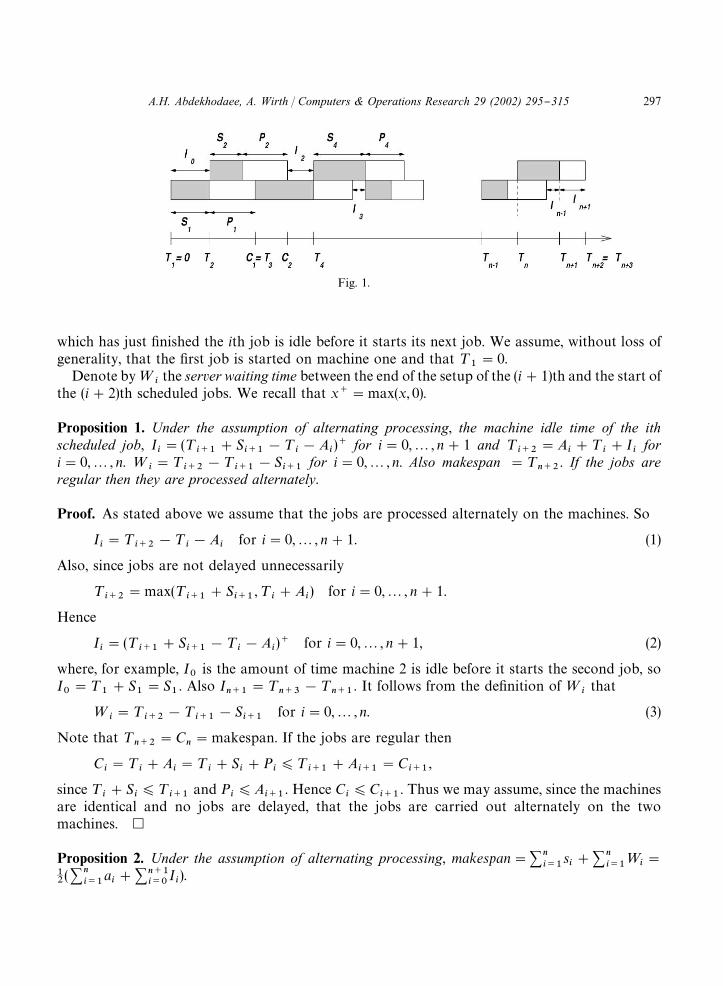
Fig. 1.

which has just "nished the ith job is idle before it starts its next job. We assume, without loss ofgenerality, that the "rst job is started on machine one and that ¹

�"0.

Denote by=�

the server waiting time between the end of the setup of the (i#1)th and the start ofthe (i#2)th scheduled jobs. We recall that x�"max(x, 0).

Proposition 1. Under the assumption of alternating processing, the machine idle time of the ithscheduled job, I

�"(¹

��#S

��!¹

�!A

�)� for i"0,2, n#1 and ¹

��"A

�#¹

�#I

�for

i"0,2, n. =�"¹

��!¹

��!S

��for i"0,2, n. Also makespan "¹

��. If the jobs are

regular then they are processed alternately.

Proof. As stated above we assume that the jobs are processed alternately on the machines. So

I�"¹

��!¹

�!A

�for i"0,2, n#1. (1)

Also, since jobs are not delayed unnecessarily

¹��

"max(¹��

#S��

, ¹�#A

�) for i"0,2, n#1.

Hence

I�"(¹

��#S

��!¹

�!A

�)� for i"0,2, n#1, (2)

where, for example, I�

is the amount of time machine 2 is idle before it starts the second job, soI�"¹

�#S

�"S

�. Also I

��"¹

��!¹

��. It follows from the de"nition of =

�that

=�"¹

��!¹

��!S

��for i"0,2, n. (3)

Note that ¹��

"C�"makespan. If the jobs are regular then

C�"¹

�#A

�"¹

�#S

�#P

�)¹

��#A

��"C

��,

since ¹�#S

�)¹

��and P

�)A

��. Hence C

�)C

��. Thus we may assume, since the machines

are identical and no jobs are delayed, that the jobs are carried out alternately on the twomachines. �

Proposition 2. Under the assumption of alternating processing, makespan"��

s�#��

��=

�"

��

(��

a�#��

��I�).

A.H. Abdekhodaee, A. Wirth / Computers & Operations Research 29 (2002) 295}315 297

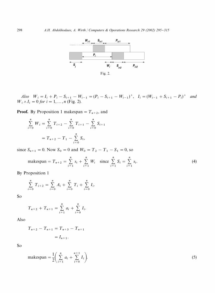
Fig. 2.

Also =�"I

�#P

�!S

��!=

��"(P

�!S

��!=

��)�, I

�"(=

��#S

��!P

�)� and

=��I

�"0 for i"1,2, n (Fig. 2).

Proof. By Proposition 1 makespan"¹��

, and

��

=�"

��

¹��

!

��

¹��

!

��

S��

"¹��

!¹�!

��

S�,

since S��

"0. Now S�"0 and =

�"¹

�!¹

�!S

�"0, so

makespan"¹��

"

��

s�#

��

=�

since��

S�"

��

s�. (4)

By Proposition 1

��

¹��

"

��

A�#

��

¹�#

��

I�.

So

¹��

#¹��

"

��

a�#

��

I�.

Also

¹��

!¹��

"¹��

!¹��

"I��

.

So

makespan"

12�

��

a�#

��

I��. (5)


Now

=�"¹

��!¹

��!S

��for i"0,2, n.

Hence

=��

"¹��

!¹�!S

�for i"1,2, n.

So

=�#=

��"¹

��!¹

�!S

��!S

�

"A�#I

�!S

��!S

�by Proposition 1

"I�#P

�!S

��.

Hence

=�"I

�#P

�!S

��!=

��for i"1,2, n. (6)

Now =��I

�"[¹

��!(¹

��#S

��)]�[¹

��!(¹

�#A

�)]"(¹

�#A

�!¹

��!S

��)��

(¹��

#S��

!¹�!A

�)�"0.

So

=�"(P

�!S

��!=

��)� and I

�"(=

��#S

��!P

�)�. �

Note that the above makespan results are intuitively clear. The makespan is the total amountof time the server spends setting up the jobs plus the sum of the server waiting times. Also,the makespan is the sum of the lengths of the jobs and the machine idle times for eachmachine.

3. Integer programming formulation

By Proposition 2, in order to minimise makespan we must minimise ��=

�.

By Proposition 2

=�"(P

�!S

��!=

��)�*P

�!S

��!=

��for i"1,2, n.

Let

x��

"�1 if job j is in the ith place in the schedule,

0 otherwise.


So the following is an integer programming formulation of the makespan minimisation problem

min��

=�

s.t.��

x��

"1, i"1,2, n,

�

��

x��

"1, j"1,2, n,

=�*

��

x��p�!

��

x��

s�!=

��i"1,2, n!1,

=�"0,

=�*

��

x��

p�!=

��,

=�*0 i"1,2, n,

x��

"0 or 1 for i, j"1,2, n.

It is clear that at the optimum =�"(P

�!S

��!=

��)� since otherwise job i#2 would be

unnecessarily delayed.We used this formulation to solve small-size problems (up to 12 jobs) with CPLEX. The

computation time proved excessive for larger problems. Nevertheless the procedure was useful innumerically verifying the correctness of the polynomial time algorithm for the equal length jobproblem.

4. Computational complexity

It is well known that the two identical parallel machine makespan minimisation problem isbinary, but not unary(strongly), NP-complete, see for example Blazewicz et al. [6]. We now showthat our problem is unary NP-complete even if we assume alternate allocation to the two machines.Since obtaining this result we learnt that Hall et al. [2] have shown the problem, P2, S1�s

�"s�C

��(all the setup times are equal) to be unary NP-complete. Kravchenko and Werner [4] showedP, S1�s

�"1�C

��is unary NP-complete (arbitrary number of identical parallel machines.) Further-

more, P2, S1�s�"1�C

��is binary NP-complete (Hall et al. [2]) and P2�s

��

��I�

is unary NP-complete (Koulamas [3]). Note that ��

��I�"2C

��!��

��a�!I

��. However, in none of the

other papers is the optimal allocation alternating.

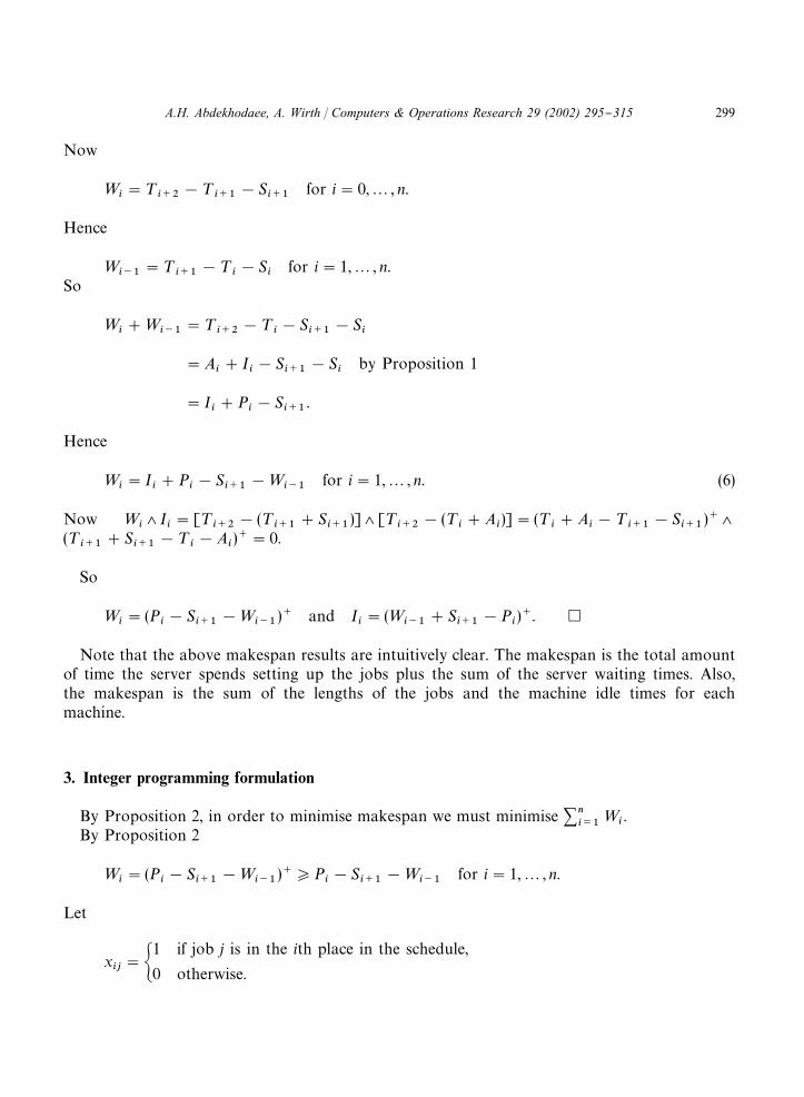
Proposition 3. The decision version of the makespan minimisation problem is NP-complete in thestrong sense.


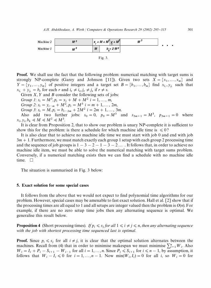
Fig. 3.

Proof. We shall use the fact that the following problem: numerical matching with target sums isstrongly NP-complete (Garey and Johnson [11]). Given two sets X"�x

�,2, x

�� and

>"�y�

,2, y�� of positive integers and a target set B"�b

�,2, b

�� "nd x

��, y

��such that

x��#y

��"b

�for each r and i

�Oi

�, j�Oj

�if rOs.

Given X,> and B consider the following sets of jobs:Group 1: s

�"M�, p

�"x

�#M#M� i"1,2, m,

Group 2: s�"y

��#M�, p

�"M� i"m#1,2, 2m,

Group 3: s�"M, p

�"b

��#2M� i"2m#1,2, 3m.

Also add two further jobs: s�"0, p

�"M� and s

��"M�, p

��"0 where

x�, y

�, b

�;M;M�;M�.

It is clear from Proposition 2, that to show our problem is unary NP-complete it is su$cient toshow this for the problem: is there a schedule for which machine idle time is )0 ?

It is also clear that to achieve no machine idle time we must start with job 0 and end with job3m#1. Furthermore, we must match exactly each group 1 setup with each group 2 processing timeand the sequence of job groups is 1!3!2!1!3!22 . It follows that, in order to achieve nomachine idle item, we must be able to solve the numerical matching with target sums problem.Conversely, if a numerical matching exists then we can "nd a schedule with no machine idletime. �

The situation is summarised in Fig. 3 below:

5. Exact solution for some special cases

It follows from the above that we would not expect to "nd polynomial time algorithms for ourproblem. However, special cases may be amenable to fast exact solution. Hall et al. [2] show that ifthe processing times are all equal to 1 and all setups are integer valued then the problem is O(n). Forexample, if there are no zero setup time jobs then any alternating sequence is optimal. Wegeneralise this result below.

Proposition 4 (Short processing times). If p�)s

�for all 1)iOj)n, then any alternating sequence

with the job with shortest processing time sequenced last is optimal.

Proof. Since p�)s

�for all iOj, it is clear that the optimal solution alternates between the

machines. Recall from (4) that in order to minimise makespan we must minimise ��=

�. Also

=�"I

�#P

�!S

��!=

��for all i"1,2, n. Since P

�)S

��for i)n!1, by assumption, it

follows that =�!I

�)0 for i"1,2, n!1. Now min(=

�, I

�)"0 for all i, so =

�"0 for


i"1,2, n!1. Hence we must minimise =�"I

�#P

�!S

��!=

��"I

�#P

�. Since

min(I�,=

�)"0 it follows that=

�"P

�. Hence any alternating sequence with the job with shortest

processing time sequenced last is optimal. �

We now consider the important special case of equal length jobs. That is, the case when a�"a for

all i. Assume further that n"2k for some k. The jobs are clearly regular and we seek to minimise��

��I�. That is, for the rest of this section we assume n"2k and a

�"a for all i.

We proceed by a series of lemmas to "nally show that an optimal solution to the equal job lengthproblem is given by S

��)S

��)2)S

�)S

�)S

�)S

�)S

)2)S

��)S

��.

Firstly we deal with the special case of short setups (s�)a/2 for all i.)

Proposition 5.

(I)��

I�)

��

��S��

!(S��

#S��

!a)�!S��

�#(S��

#S��

!a)��,�. (7)

(II) ��

�S��

!S��

�)�)

��

��S��

!S��

�#2(S��

#S��

!a)��. (8)

(III) ��

�S��

!S��

�, that is, �0!S��#�S

�!S

��#2#�S

��!0� is minimised by hav-

ing �S�

, S�

,2, S��

��-shaped (that is S�)S

�)2)S

��, S

��*S

��2*S

��)

and S��

)S��

for all i, j.

(IV) ��

I�*2

�max��

S��

. (9)

(V) If s�)a/2 for all i (short setups) then ��

��I�

(that is makespan) is minimised if�S

�, S

�,2, S

�� is �-shaped and S

��)S

��for all i, j, that is, S

��)S

��, for all odd

and even jobs.

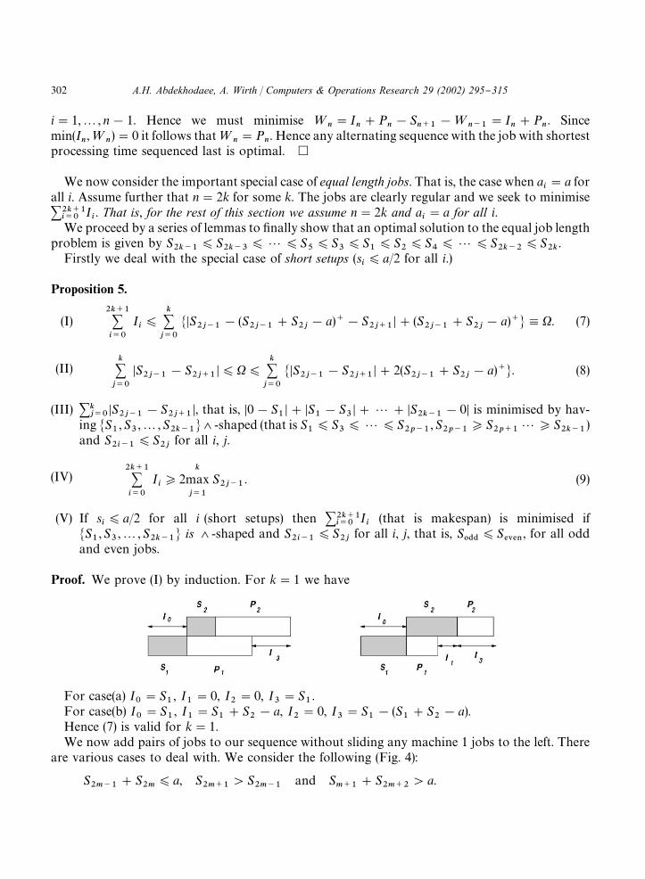
Proof. We prove (I) by induction. For k"1 we have

For case(a) I�"S

�, I

�"0, I

�"0, I

�"S

�.

For case(b) I�"S

�, I

�"S

�#S

�!a, I

�"0, I

�"S

�!(S

�#S

�!a).

Hence (7) is valid for k"1.We now add pairs of jobs to our sequence without sliding any machine 1 jobs to the left. There

are various cases to deal with. We consider the following (Fig. 4):

S��

#S��

)a, S��

'S��

and S��

#S��

'a.


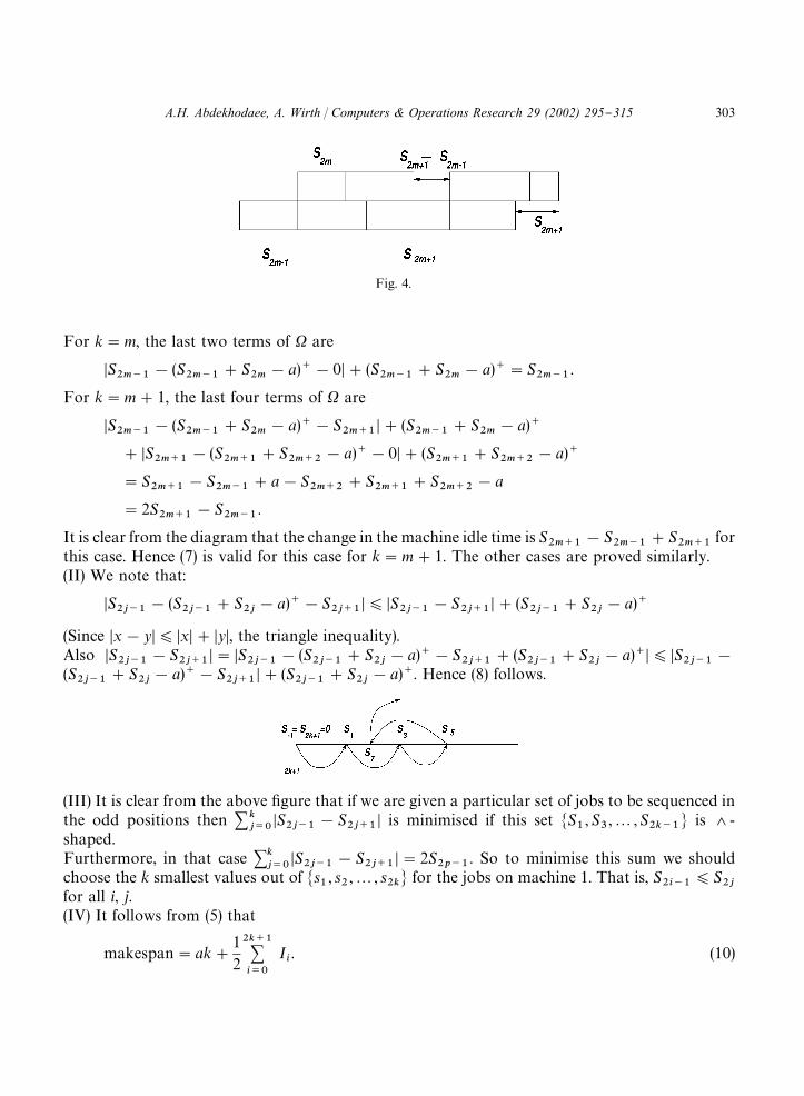
Fig. 4.

For k"m, the last two terms of � are

�S��

!(S��

#S��

!a)�!0�#(S��

#S��

!a)�"S��

.

For k"m#1, the last four terms of � are

�S��

!(S��

#S��

!a)�!S��

�#(S��

#S��

!a)�

#�S��

!(S��

#S��

!a)�!0�#(S��

#S��

!a)�

"S��

!S��

#a!S��

#S��

#S��

!a

"2S��

!S��

.

It is clear from the diagram that the change in the machine idle time is S��

!S��

#S��

forthis case. Hence (7) is valid for this case for k"m#1. The other cases are proved similarly.(II) We note that:

�S��

!(S��

#S��

!a)�!S��

�)�S��

!S��

�#(S��

#S��

!a)�

(Since �x!y�)�x�#�y�, the triangle inequality).Also �S

��!S

��"�S

��!(S

��#S

��!a)�!S

��#(S

��#S

��!a)��)�S

��!

(S��

#S��

!a)�!S��

�#(S��

#S��

!a)�. Hence (8) follows.

(III) It is clear from the above "gure that if we are given a particular set of jobs to be sequenced inthe odd positions then ��

��S

��!S

�� is minimised if this set �S

�, S

�,2, S

�� is �-

shaped.Furthermore, in that case ��

��S

��!S

��"2S

��. So to minimise this sum we should

choose the k smallest values out of �s�

, s�

,2, s��

� for the jobs on machine 1. That is, S��

)S��

for all i, j.(IV) It follows from (5) that

makespan"ak#

12��

I�. (10)


Now suppose that S��

*S��

for j"1,2, k. Also (p!1) jobs precede job 2p!1 on machine1. So

¹�

*a(p!1)#S��

. (11)

Further, (k!p#1) jobs start at or after ¹��

on machine 2. So

makespan*¹�

#(k!p#1)a. (12)

It follows from (10)}(12) that

ak#

12��

I�*ak#S

��.

So

��

I�*2S

��.

(V) If s�)a/2 for all i then (S

��#S

��!a)�"0 for all j. So �"��

��S

��!S

�� by (8).

Furthermore, � is minimised under condition of (III) with value 2S��

. Hence, by (I), (IV) andthe proof of (III):

2S��

)min��

I�)min �"2 min

��

�S��

!S��

�"2S��

.

Thus ��

I�

is minimised when �S�

, S�

,2, S��

� is �-shaped and S��

)S��

for all i, j andequals to 2s

�. �

Now we turn to the general equal job length problem.

Lemma 6. For the equal length job problem, suppose that jobs on machine one are arranged indecreasing order of setup time. That is we have S

�*S

�*S

�*2*S

��. Then

makespan"S�#(S

�#S

�!a)�#2#(S

��#S

��!a)�#ka.

Proof. By Proposition 2 =�"(P

�!S

��!=

��)�"(a!S

�!S

��!=

��)�. If S

�*S

�*

S�*2*S

��then

=�"(a!S

�!S

�)� (since =

�"0, see proof of Proposition 2).

Now I�"(=

��#S

��#S

�!a)� by Proposition 2

/I�"�

(S�#S

�!a)� if =

�"0,

(S�#S

�!a#a!S

�!S

�)�"(S

�!S

�)�"0 if =

�'0.

So, in both cases I�"(S

�#S

�!a)� (since, if =

�'0 then 0*I

�*(S

�#S

�!a)�*0).

Similarly

I"�

(S#S

�!a)� if =

�"0,

(S#S

�!a#a!S

!S

�!=

�)�)(S

�!S

�)�"0 if =

�'0,


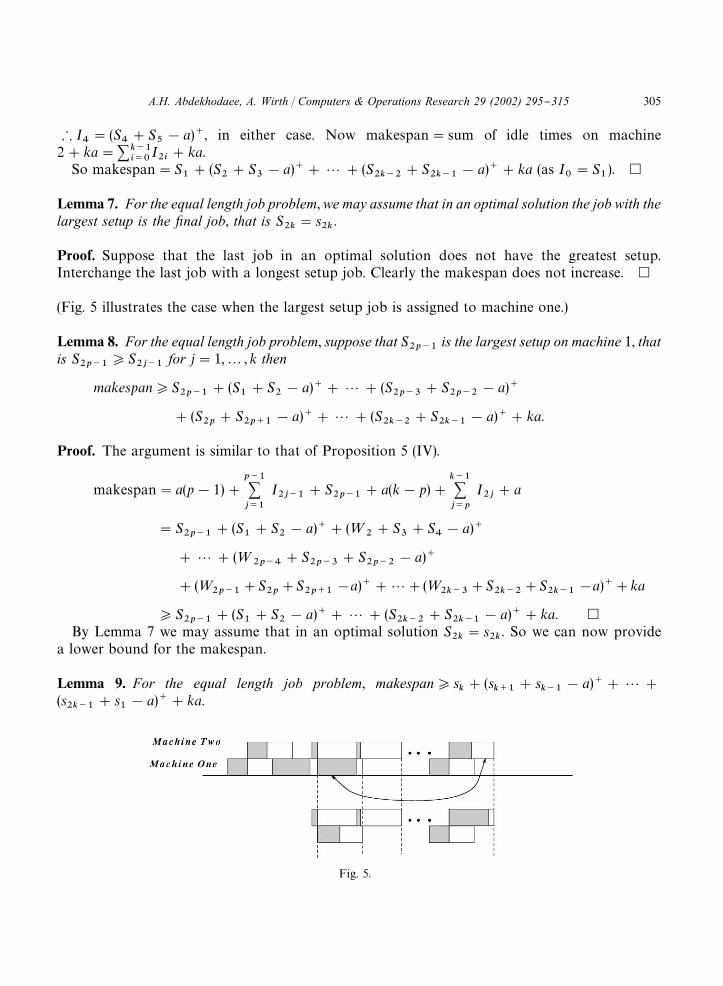
Fig. 5.

/I"(S

#S

�!a)�, in either case. Now makespan"sum of idle times on machine

2#ka"��

I��

#ka.So makespan"S

�#(S

�#S

�!a)�#2#(S

��#S

��!a)�#ka (as I

�"S

�). �

Lemma 7. For the equal length job problem,we may assume that in an optimal solution the job with thelargest setup is the xnal job, that is S

��"s

��.

Proof. Suppose that the last job in an optimal solution does not have the greatest setup.Interchange the last job with a longest setup job. Clearly the makespan does not increase. �

(Fig. 5 illustrates the case when the largest setup job is assigned to machine one.)

Lemma 8. For the equal length job problem, suppose that S��

is the largest setup on machine 1, thatis S

��*S

��for j"1,2, k then

makespan*S��

#(S�#S

�!a)�#2#(S

��#S

��!a)�

#(S�

#S��

!a)�#2#(S��

#S��

!a)�#ka.

Proof. The argument is similar to that of Proposition 5 (IV).

makespan"a(p!1)#��

I��

#S��

#a(k!p)#��

I��

#a

"S��

#(S�#S

�!a)�#(=

�#S

�#S

!a)�

#2#(=��

#S��

#S��

!a)�

#(=��

#S�

#S��

!a)�#2#(=��

#S��

#S��

!a)�#ka

*S��

#(S�#S

�!a)�#2#(S

��#S

��!a)�#ka. �

By Lemma 7 we may assume that in an optimal solution S��

"s��

. So we can now providea lower bound for the makespan.

Lemma 9. For the equal length job problem, makespan*s�#(s

��#s

��!a)�#2#

(s��

#s�!a)�#ka.


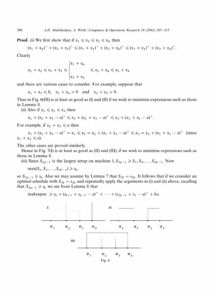
Fig. 6.

Proof. (i) We "rst show that if ��)�

�)�

�)�

then

(��#�

)�#(�

�#�

�)�)(�

�#�

�)�#(�

�#�

)�)(�

�#�

�)�#(�

�#�

)�.

Clearly

��#�

�)�

�#�

�)�

��#�

)�

�#�

)�

�#�

��#�

�

and there are various cases to consider. For example, suppose that

��#�

�)0, �

�#�

'0 and �

�#�

�'0.

Thus in Fig. 6(III) is at least as good as (I) and (II) if we wish to minimise expressions such as thosein Lemma 8.

(ii) Also if ��)�

�)�

�then

��#(�

�#�

�!a)�)�

�#(�

�#�

�!a)�)�

�#(�

�#�

�!a)�.

For example, if ��#�

�)a then

��#(�

�#�

�!a)�"�

�)�

�"�

�#(�

�#�

�!a)�)�

�"�

�#(�

�#�

�!a)� (since

��#�

�)a).

The other cases are proved similarly.Hence in Fig. 7(I) is at least as good as (II) and (III), if we wish to minimise expressions such as

those in Lemma 8.(iii) Since S

��is the largest setup on machine 1, S

��*S

�, S

�,2, S

��. Now

max(S�

, S�

,2, S��

)*s�,

so S��

*s�. Also we may assume by Lemma 7 that S

��"s

��. It follows that if we consider an

optimal schedule with S��

"s��

and repeatedly apply the arguments in (i) and (ii) above, recallingthat S

��*s

�we see from Lemma 8 that

makespan *s�#(s

��#s

��!a)�#2#(s

��#s

�!a)�#ka.


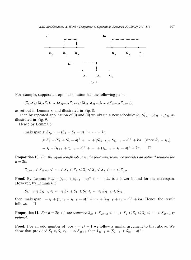
Fig. 7.

For example, suppose an optimal solution has the following pairs:

(S�

, S�

), (S�

, S

),2, (S��

, S��

), (S�

, S��

),2, (S��

, S��

),

as set out in Lemma 8, and illustrated in Fig. 8.Then by repeated application of (i) and (ii) we obtain a new schedule: S�

�, S�

�,2, S�

��, S�

��as

illustrated in Fig. 9.Hence by Lemma 8

makespan*S��

#(S�#S

�!a)�#2#ka

*S��#(S�

�#S�

�!a)�#2#(S�

��#S

��!a)�#ka (since S�

�"s

��)

"s�#(s

��#s

��!a)�#2#(s

��#s

�!a)�#ka. �

Proposition 10. For the equal length job case, the following sequence provides an optimal solution forn"2k:

S��

)S��

)2)S�)S

�)S

�)S

�)S

)2)S

��.

Proof. By Lemma 9 s�#(s

��#s

��!a)�#2#ka is a lower bound for the makespan.

However, by Lemma 6 if

S��

)S��

)2)S�)S

�)S

�)2)S

��)S

��,

then makespan "s�#(s

��#s

��!a)�#2#(s

��#s

�!a)�#ka. Hence the result

follows. �

Proposition 11. For n"2k#1 the sequence S��

)S��

)2)S�)S

�)S

�)2)S

��is

optimal.

Proof. For an odd number of jobs n"2k#1 we follow a similar argument to that above. Weshow that provided S

�)S

�)2)S

��then I

��"(S

��#S

��!a)�.


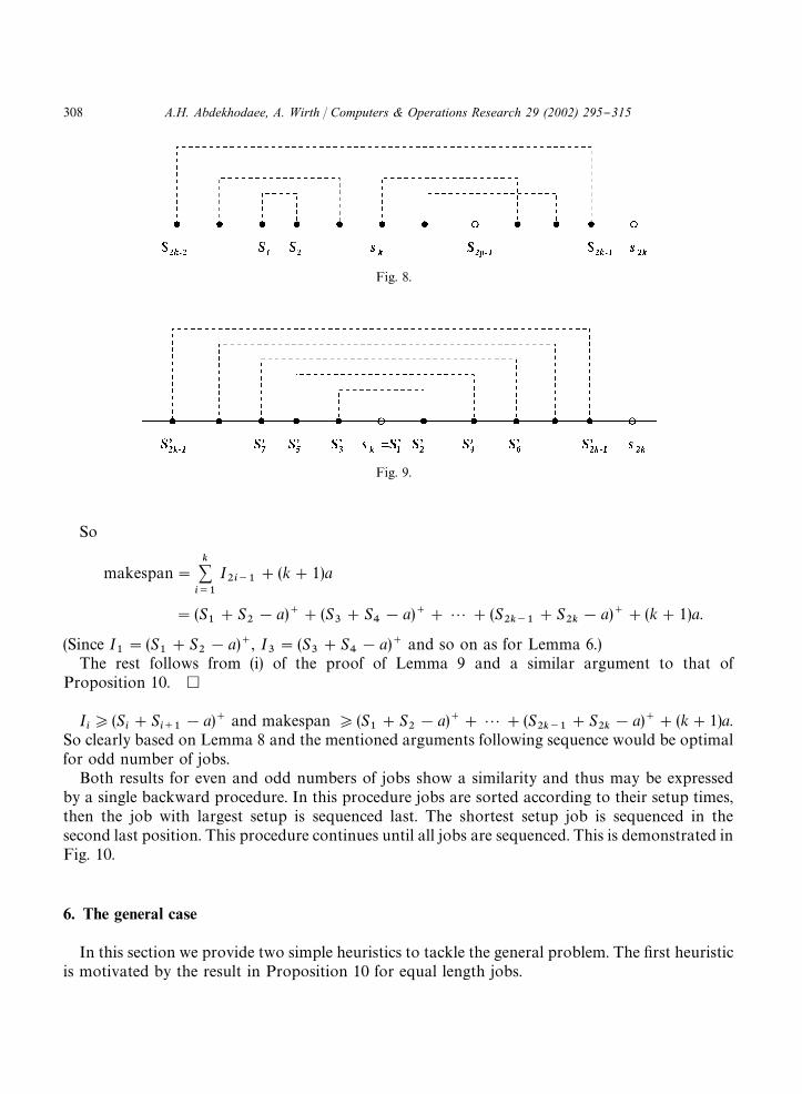
Fig. 8.

Fig. 9.

So

makespan"

��

I��

#(k#1)a

"(S�#S

�!a)�#(S

�#S

!a)�#2#(S

��#S

��!a)�#(k#1)a.

(Since I�"(S

�#S

�!a)�, I

�"(S

�#S

!a)� and so on as for Lemma 6.)

The rest follows from (i) of the proof of Lemma 9 and a similar argument to that ofProposition 10. �

I�*(S

�#S

��!a)� and makespan *(S

�#S

�!a)�#2#(S

��#S

��!a)�#(k#1)a.

So clearly based on Lemma 8 and the mentioned arguments following sequence would be optimalfor odd number of jobs.

Both results for even and odd numbers of jobs show a similarity and thus may be expressedby a single backward procedure. In this procedure jobs are sorted according to their setup times,then the job with largest setup is sequenced last. The shortest setup job is sequenced in thesecond last position. This procedure continues until all jobs are sequenced. This is demonstrated inFig. 10.

6. The general case

In this section we provide two simple heuristics to tackle the general problem. The "rst heuristicis motivated by the result in Proposition 10 for equal length jobs.


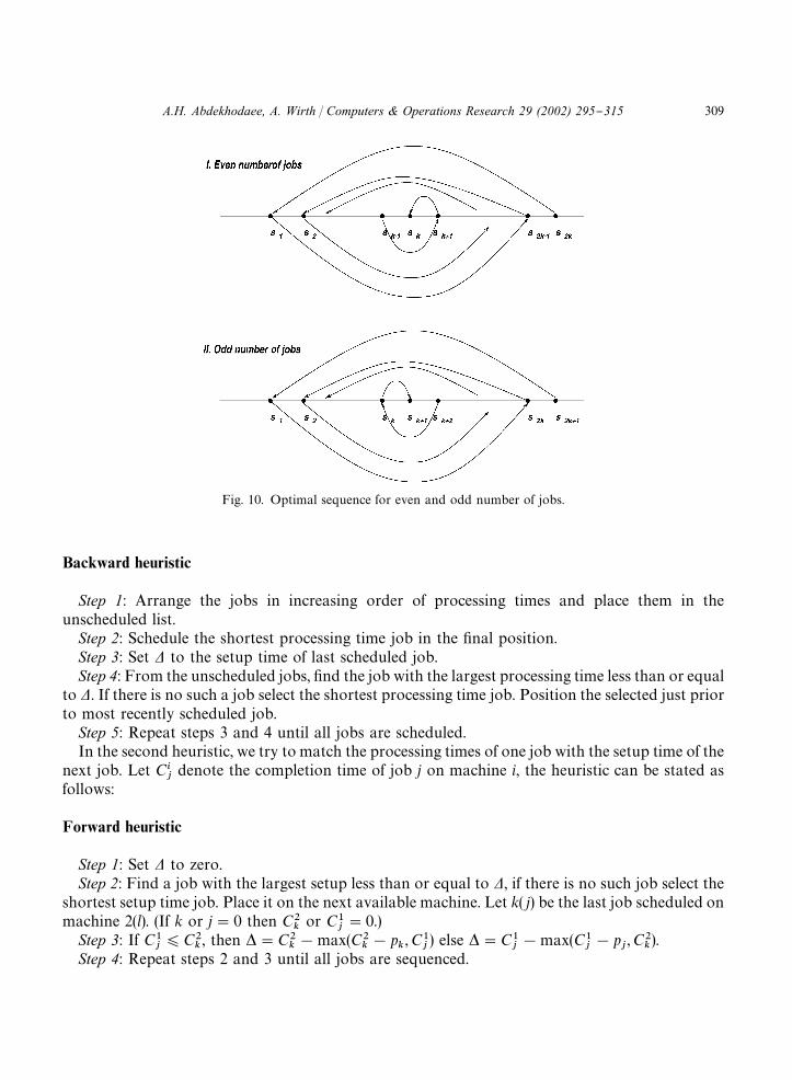
Fig. 10. Optimal sequence for even and odd number of jobs.

Backward heuristic

Step 1: Arrange the jobs in increasing order of processing times and place them in theunscheduled list.Step 2: Schedule the shortest processing time job in the "nal position.Step 3: Set � to the setup time of last scheduled job.Step 4: From the unscheduled jobs, "nd the job with the largest processing time less than or equal

to �. If there is no such a job select the shortest processing time job. Position the selected just priorto most recently scheduled job.Step 5: Repeat steps 3 and 4 until all jobs are scheduled.In the second heuristic, we try to match the processing times of one job with the setup time of the

next job. Let C��

denote the completion time of job j on machine i, the heuristic can be stated asfollows:

Forward heuristic

Step 1: Set � to zero.Step 2: Find a job with the largest setup less than or equal to �, if there is no such job select the

shortest setup time job. Place it on the next available machine. Let k( j) be the last job scheduled onmachine 2(l). (If k or j"0 then C�

�or C�

�"0.)

Step 3: If C��)C�

�, then �"C�

�!max(C�

�!p

�, C�

�) else �"C�

�!max(C�

�!p

�, C�

�).

Step 4: Repeat steps 2 and 3 until all jobs are sequenced.


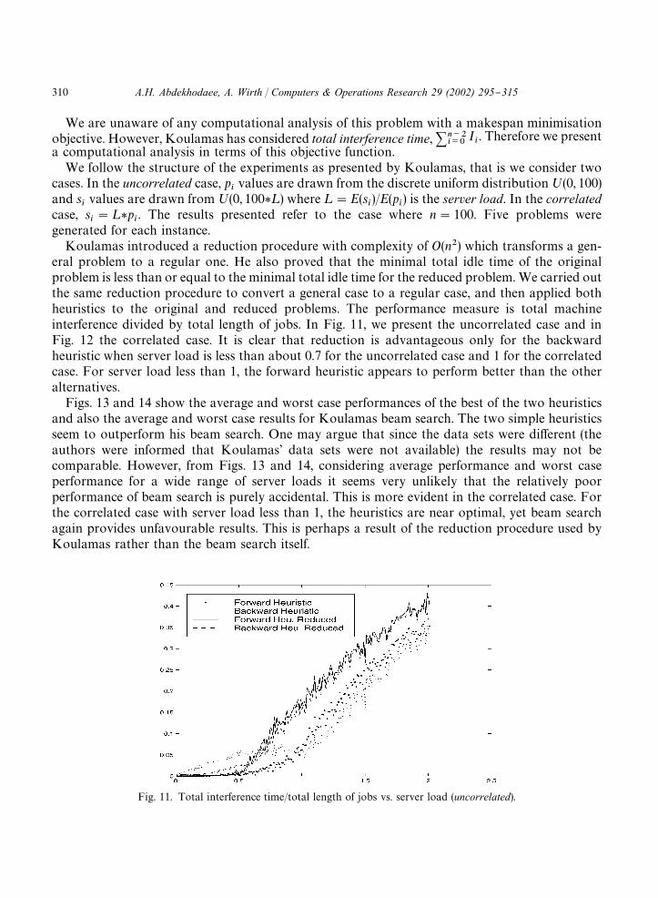
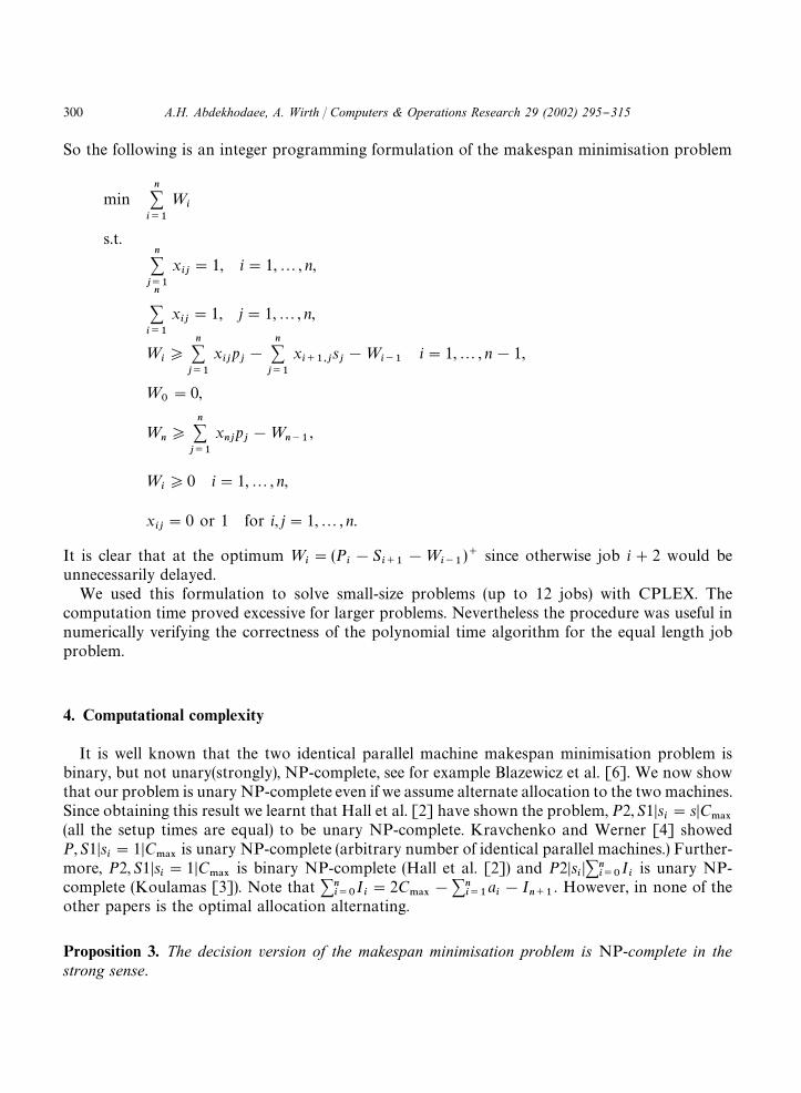
Fig. 11. Total interference time/total length of jobs vs. server load (uncorrelated).

We are unaware of any computational analysis of this problem with a makespan minimisationobjective. However, Koulamas has considered total interference time, ��

��I�. Therefore we present

a computational analysis in terms of this objective function.We follow the structure of the experiments as presented by Koulamas, that is we consider two

cases. In the uncorrelated case, p�

values are drawn from the discrete uniform distribution;(0, 100)and s

�values are drawn from;(0, 100*¸) where ¸"E(s

�)/E(p

�) is the server load. In the correlated

case, s�"¸*p�

. The results presented refer to the case where n"100. Five problems weregenerated for each instance.

Koulamas introduced a reduction procedure with complexity of O(n�) which transforms a gen-eral problem to a regular one. He also proved that the minimal total idle time of the originalproblem is less than or equal to the minimal total idle time for the reduced problem. We carried outthe same reduction procedure to convert a general case to a regular case, and then applied bothheuristics to the original and reduced problems. The performance measure is total machineinterference divided by total length of jobs. In Fig. 11, we present the uncorrelated case and inFig. 12 the correlated case. It is clear that reduction is advantageous only for the backwardheuristic when server load is less than about 0.7 for the uncorrelated case and 1 for the correlatedcase. For server load less than 1, the forward heuristic appears to perform better than the otheralternatives.

Figs. 13 and 14 show the average and worst case performances of the best of the two heuristicsand also the average and worst case results for Koulamas beam search. The two simple heuristicsseem to outperform his beam search. One may argue that since the data sets were di!erent (theauthors were informed that Koulamas' data sets were not available) the results may not becomparable. However, from Figs. 13 and 14, considering average performance and worst caseperformance for a wide range of server loads it seems very unlikely that the relatively poorperformance of beam search is purely accidental. This is more evident in the correlated case. Forthe correlated case with server load less than 1, the heuristics are near optimal, yet beam searchagain provides unfavourable results. This is perhaps a result of the reduction procedure used byKoulamas rather than the beam search itself.


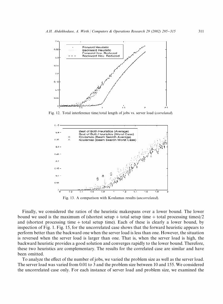
Fig. 12. Total interference time/total length of jobs vs. server load (correlated).

Fig. 13. A comparison with Koulamas results (uncorrelated).

Finally, we considered the ratios of the heuristic makespans over a lower bound. The lowerbound we used is the maximum of (shortest setup#total setup time#total processing times)/2and (shortest processing time#total setup time). Each of these is clearly a lower bound, byinspection of Fig. 1. Fig. 15, for the uncorrelated case shows that the forward heuristic appears toperform better than the backward one when the server load is less than one. However, the situationis reversed when the server load is larger than one. That is, when the server load is high, thebackward heuristic provides a good solution and converges rapidly to the lower bound. Therefore,these two heuristics are complementary. The results for the correlated case are similar and havebeen omitted.

To analyze the e!ect of the number of jobs, we varied the problem size as well as the server load.The server load was varied from 0.01 to 3 and the problem size between 10 and 155. We consideredthe uncorrelated case only. For each instance of server load and problem size, we examined the


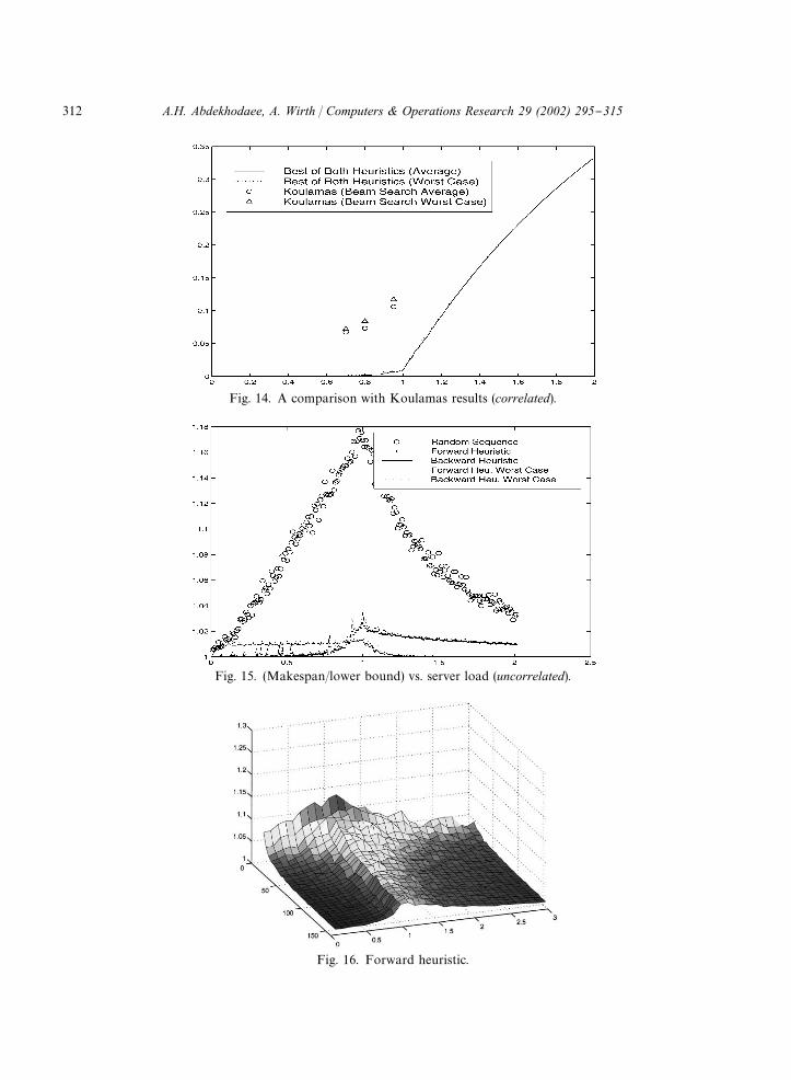
Fig. 14. A comparison with Koulamas results (correlated).

Fig. 15. (Makespan/lower bound) vs. server load (uncorrelated).

Fig. 16. Forward heuristic.


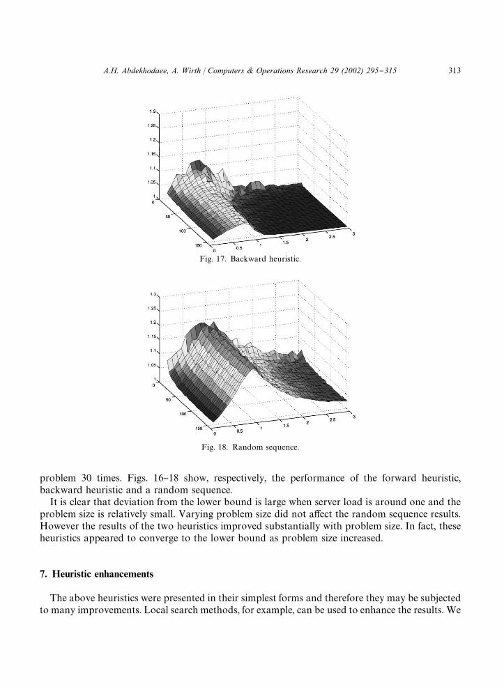
Fig. 17. Backward heuristic.

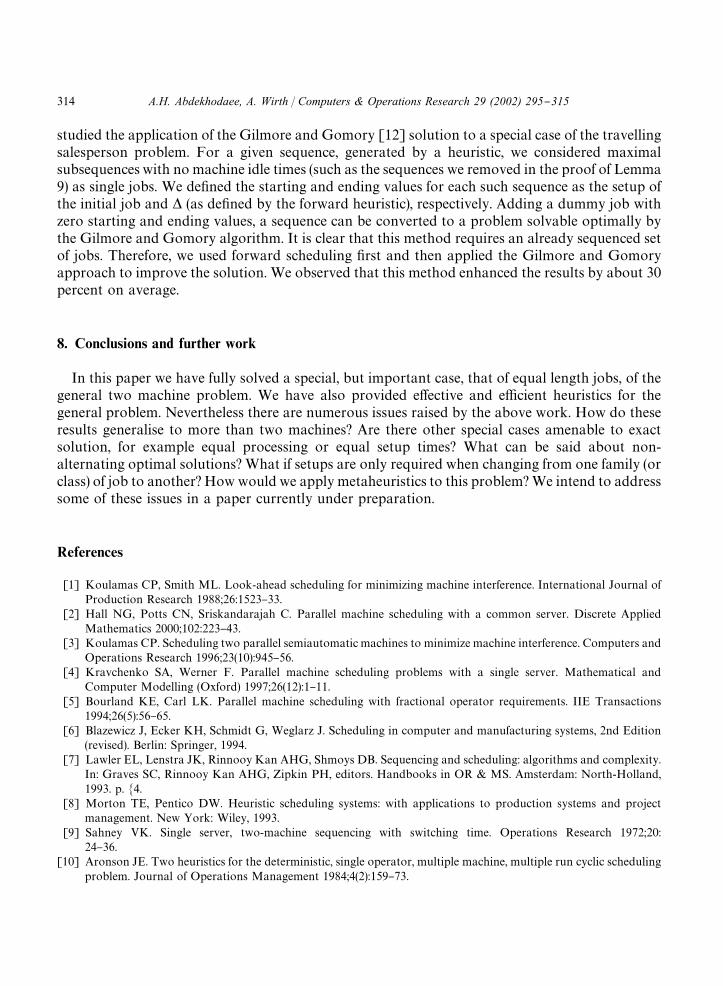
Fig. 18. Random sequence.

problem 30 times. Figs. 16}18 show, respectively, the performance of the forward heuristic,backward heuristic and a random sequence.

It is clear that deviation from the lower bound is large when server load is around one and theproblem size is relatively small. Varying problem size did not a!ect the random sequence results.However the results of the two heuristics improved substantially with problem size. In fact, theseheuristics appeared to converge to the lower bound as problem size increased.

7. Heuristic enhancements

The above heuristics were presented in their simplest forms and therefore they may be subjectedto many improvements. Local search methods, for example, can be used to enhance the results. We


studied the application of the Gilmore and Gomory [12] solution to a special case of the travellingsalesperson problem. For a given sequence, generated by a heuristic, we considered maximalsubsequences with no machine idle times (such as the sequences we removed in the proof of Lemma9) as single jobs. We de"ned the starting and ending values for each such sequence as the setup ofthe initial job and � (as de"ned by the forward heuristic), respectively. Adding a dummy job withzero starting and ending values, a sequence can be converted to a problem solvable optimally bythe Gilmore and Gomory algorithm. It is clear that this method requires an already sequenced setof jobs. Therefore, we used forward scheduling "rst and then applied the Gilmore and Gomoryapproach to improve the solution. We observed that this method enhanced the results by about 30percent on average.

8. Conclusions and further work

In this paper we have fully solved a special, but important case, that of equal length jobs, of thegeneral two machine problem. We have also provided e!ective and e$cient heuristics for thegeneral problem. Nevertheless there are numerous issues raised by the above work. How do theseresults generalise to more than two machines? Are there other special cases amenable to exactsolution, for example equal processing or equal setup times? What can be said about non-alternating optimal solutions? What if setups are only required when changing from one family (orclass) of job to another? How would we apply metaheuristics to this problem? We intend to addresssome of these issues in a paper currently under preparation.

References

[1] Koulamas CP, Smith ML. Look-ahead scheduling for minimizing machine interference. International Journal ofProduction Research 1988;26:1523}33.

[2] Hall NG, Potts CN, Sriskandarajah C. Parallel machine scheduling with a common server. Discrete AppliedMathematics 2000;102:223}43.

[3] Koulamas CP. Scheduling two parallel semiautomatic machines to minimize machine interference. Computers andOperations Research 1996;23(10):945}56.

[4] Kravchenko SA, Werner F. Parallel machine scheduling problems with a single server. Mathematical andComputer Modelling (Oxford) 1997;26(12):1}11.

[5] Bourland KE, Carl LK. Parallel machine scheduling with fractional operator requirements. IIE Transactions1994;26(5):56}65.

[6] Blazewicz J, Ecker KH, Schmidt G, Weglarz J. Scheduling in computer and manufacturing systems, 2nd Edition(revised). Berlin: Springer, 1994.

[7] Lawler EL, Lenstra JK, Rinnooy Kan AHG, Shmoys DB. Sequencing and scheduling: algorithms and complexity.In: Graves SC, Rinnooy Kan AHG, Zipkin PH, editors. Handbooks in OR & MS. Amsterdam: North-Holland,1993. p. �4.

[8] Morton TE, Pentico DW. Heuristic scheduling systems: with applications to production systems and projectmanagement. New York: Wiley, 1993.

[9] Sahney VK. Single server, two-machine sequencing with switching time. Operations Research 1972;20:24}36.

[10] Aronson JE. Two heuristics for the deterministic, single operator, multiple machine, multiple run cyclic schedulingproblem. Journal of Operations Management 1984;4(2):159}73.


[11] Garey MR, Johnson DS. Computers and intractability: a guide to the theory of NP-completeness. San Francisco:W.H. Freeman, 1979.

[12] Gilmore PC, Gomory RE. Sequencing a one state variable machine: a solvable case of the travelling salesmanproblem. Operations Research 1964;12:655}79.

Amir H. Abdekhodaee received his bachelor degree in Industrial Engineering from Amirkabir University, Tehran, Iran.He obtained a Master of Engineering Science degree from the University of New South Wales, Sydney, Australia. He hasrecently completed his Ph.D. at the University of Melbourne. His areas of interest are scheduling, combinatorialoptimization and computer simulation.AndrewWirth is a member of the Department of Mechanical and Manufacturing Engineering and the Mathematics for

Engineers program at the University of Melbourne. His current research interests are in scheduling and networksurvivability. His publications include articles in the Proceedings of the American Mathematical Society, Journal of theLondon Mathematical Society, Zeitschrift fur Operations Research, Omega, Decision Support Systems, Journal of BusinessFinance and Accounting, Engineering Costs and Production Economics, International Journal of Production Research,Journal of the Operation Research Society and the European Journal of Operational Research.


Documents

Scheduling parallel machines with a single server: some solvable cases and heuristics