Ann Oper Res (2012) 196:491–516DOI 10.1007/s10479-012-1098-1

Scheduling problems with position dependent jobprocessing times: computational complexity results

Radosław Rudek

Published online: 29 February 2012© The Author(s) 2012. This article is published with open access at Springerlink.com

Abstract In this paper, we analyse single machine scheduling problems with learning andaging effects to minimize one of the following objectives: the makespan with release dates,the maximum lateness and the number of late jobs. The phenomena of learning and aging aremodeled by job processing times described by non-increasing (learning) or non-decreasing(aging) functions dependent on the number of previously processed jobs, i.e., a job positionin a sequence. We prove that the considered problems are strongly NP-hard even if job pro-cessing times are described by simple linear functions dependent on a number of processedjobs. Additionally, we show a property of equivalence between problems with learning andaging models. We also prove that if the function describing decrease/increase of a job pro-cessing time is the same for each job then the problems with the considered objectives arepolynomially solvable even if the function is arbitrary. Therefore, we determine the bound-ary between polynomially solvable and strongly NP-hard cases.

Keywords Scheduling · Learning effect · Aging effect · Computational complexity

1 Introduction

Changeability is a characteristic feature of many real-life systems (e.g., manufacturing, in-dustrial, computer, etc.) that in general can be classified as an improvement or a degradationof such a system. The improvement was for the first time discovered and described in aquantitative form in aircraft industry by Wright (1936). He observed that the total hours toassemble an aircraft decreases as the number of assembled aircrafts increases due to theincreasing experience of workers (the learning effect). Therefore, the same resources allowto produce more units in a shorter period of time. On this basis, Wright (1936) formulateda relation, called learning curve, where the time p(v) required to produce the vth unit wasdefined as follows:

R. Rudek (�)Wrocław University of Economics, Komandorska 118/120, 53-345 Wrocław, Polande-mail: radoslaw.rudek@ue.wroc.pl

492 Ann Oper Res (2012) 196:491–516

p(v) = avα, (1)

where a is the time required to produce the first unit and α ≤ 0 is the learning index.It is not surprising that the learning effect has attracted particular attention in the aircraft

industry earlier than in any other on account of the high cost of aircrafts (Kerzner 1998).The benefits following the theory of the learning effect were soon recognized by USA WarProduction Board and the methodology proposed by Wright was used to plan the produc-tion of airplanes for the World War II needs (see Roberts 1983). Further empirical studieson the learning effect carried out within the last 60 years horizon proved its significant im-pact on productivity in manufacturing systems specialized in Hi-Tech electronic equipment(Adler and Clark 1991), memory chips and circuit boards (Webb 1994), electronic guid-ance systems (Kerzner 1998) and in many others (e.g. Carlson and Rowe 1976; Cochran1960; Holzer and Riahi-Belkaoui 1986; Jaber and Bonney 1999; Lien and Rasch 2001;Yelle 1979). Most of these investigations confirmed the high accuracy of (1), however, theyalso revealed that some systems are more precisely described by other characteristics (learn-ing curves), e.g., S-shaped, Stanford-B or DeJong (see Holzer and Riahi-Belkaoui 1986;Jaber and Bonney 1999; Lien and Rasch 2001).

In general the learning effect takes place in typical human activity environments or in au-tomatized manufacturing, where a human support for machines is needed during activitiessuch as operating, controlling, setup, cleaning, maintaining, failure removal, etc. Althoughlearning can cease with time, it is often aroused by such factors as new inexperienced em-ployees, extension of an assortment, new machines, more refined equipment, software up-date or general changes of the production environment (Biskup 2008).

However, the learning effect is not limited to the areas dominated by human. For instance,highly automatized manufacturing systems may benefit on the fact that if a machine doesthe same job repetitively, then the knowledge from the previous iterations can be used toimprove the performance of a system when the job is processed the next time. An exampleof such method is iterative learning control that compensates a repetitive error in a robotmotion control (see Arimoto et al. 1984).

The learning effect also occurs in machine learning and artificial intelligence. Forinstance, reinforcement learning algorithms, that usually learn and operate on-line (seeWhiteson and Stone 2004), improve their efficiency on the basis of interactions withan environments (learning-by-doing). Thus, the performances of the systems optimizedby such algorithms improve in their succeeding iterations (e.g., Busoniu et al. 2008;Janiak and Rudek 2011).

The described learning effect that is a result of repeating similar operations (learning-by-doing) is called an autonomous learning (e.g., Yelle 1979). The theory of the learn-ing effect enables (based on (1)) for efficient estimation of the variable production timeand/or cost caused by learning. Thus, it allows to improve lot-sizes, worker manage-ment, energy/resource consumption, etc. (e.g., Keachie and Fontana 1966; Kerzner 1998;Li and Cheng 1994; Webb 1994). Nevertheless, it is not possible to optimize time and/orcost objectives beyond reductions resulting from learning-by-doing (Biskup 2008). It fol-lows from the innate nature of autonomous learning and from an assumption of identicalproducts, therefore, control (management) abilities provided by the theory of the learningeffect are significantly limited.

However, in many manufacturing systems jobs (e.g., products) are not identical, but sim-ilar and the time required to process each of them can differ. This rigorous constraint onidentical jobs was relaxed by Biskup (1999). Based on (1), he assumed that the time pj (v)

required to process job (e.g., to produce unit) j decreases as the number v of processed

Ann Oper Res (2012) 196:491–516 493

similar (not necessarily identical) jobs increases and this relation was described as follows:

pj (v) = ajvα, (2)

where aj is the time required to process job j if no learning exists (i.e., it is processed as thefirst one). On this basis, a new model was obtained that offers an additional control variable,i.e., sequence of processed jobs. Thus, it became possible to optimize production objectivessuch as the maximum completion time of jobs, the maximum lateness or the number of latejobs (e.g. Bachman and Janiak 2004; Cheng and Wang 2000; Cheng et al. 2008; Lee and Lai2011; Lee et al. 2010; Wu et al. 2007; Wang and Wang 2011; Yang and Kuo 2009; Zhanget al. 2011), which were beyond control using the theory of the learning effect. Therefore,fundamental for this approach is that control decisions (schedule) do not influence learning(that anyway in many cases is impossible), but they allow to efficiently utilize learningabilities of the system to optimize given objectives. Thus, not surprisingly, this directionof research has attracted particular attention in the scheduling theory, especially in issuesdevoted to manufacturing systems (for survey see Biskup 2008).

On the other hand, degradation of a system can be caused by deterioration/aging of ma-chines (understood as lathe machines, chemical cleaning baths, etc.) or fatigue of humanworkers that affects the production parameters such as time/cost required to produce a sin-gle unit (e.g. Dababneh et al. 2001; Eilon 1964; Mandich 2003; Stanford and Lister 2004).Similarly as for learning systems, the objectives of deteriorating systems can also be con-trolled (in a specified range) by a schedule of processed jobs. In the scheduling theory thereare two approaches to model deterioration. Although both of them describe the dependencybetween job processing times and deteriorating factors, for each of them the deterioratingfactor is represented by different parameters. Namely, the first approach, called deterio-rating effect, assumes that the job processing times are non-decreasing functions of theirstarting times and it has been extensively studied in the last decade (see Cheng et al. 2004and Gawiejnowicz 2008).

However, scheduling models consistent with this approach are not relevant to manyreal-life industrial problems. It is especially significant for environments, where deterio-ration does not take place (or is negligible) during idle times of machines (workers), e.g.,caused by different release dates of jobs. Such inconveniences are absent in the secondapproach, called aging/fatigue effect, in which job processing times are described by non-decreasing functions dependent on the actual condition (fatigue) of machines affected by al-ready processed jobs (e.g., Cheng et al. 2010; Janiak and Rudek 2010; Kuo and Yang 2008;Rudek and Rudek 2011; Yang et al. 2010). Similarity of jobs usually allows to assumethat each of them has the same impact on the fatigue of a machine (e.g. Cheng et al. 2008;Gawiejnowicz 1996; Mosheiov 2001; Yang and Yang 2010). Therefore, we will focus on thisapproach, where the time pj (v) required to process job j increases together with the num-ber v of processed jobs. This relation can be described by (2), where α ≥ 0 (see Mosheiov2001).

In this paper, we analyse computational complexity of single machine scheduling prob-lems with linear models of learning/aging and the following minimization objectives: themaximum lateness, the makespan with release dates and additionally the number of late jobs.The main theoretical result of this paper is to prove that the considered problems are stronglyNP-hard with linear functions of job processing times. Although the maximum lateness min-imization scheduling problems with position dependent job processing times are broadlydiscussed (e.g., Bachman and Janiak 2004; Cheng and Wang 2000; Cheng et al. 2008;Lee and Lai 2011), their computational complexity is not fully determined. Therefore, to

494 Ann Oper Res (2012) 196:491–516

complement these results and to make their analysis coherent, we will determine their com-putational complexity. Namely, we will prove that the problems even with the simplestpossible (nontrivial) mathematical models of job processing times are strongly NP-hard.Moreover, it will be shown that if the models are simpler (then trivial) the related problemsare polynomially solvable. Thus, we will determine the boundary between the polynomialsolvability of the problems and their strong NP-hardness. Thereby, we will complement theresults provided inter alia by Bachman and Janiak (2004) and Cheng and Wang (2000) andforemost complete the results concerning the maximum lateness minimization with positiondependent job processing times. Since, any NP-hardness proof is more significant if it isdone for the simplest possible problem as it is done in this paper.

On the other hand, the practical aspect of this research is to show that the maximumacceptable simplification of job processing time functions (by their linearization) does notlead to decreasing complexity of the considered problems. Therefore, it does not lead todecreasing effort required to obtain optimal control decisions but rather to decreasing theiraccuracy. Additionally, we also prove that the considered problems with an arbitrary func-tions describing decreasing/increasing of a job processing time are polynomially solvable ifthe functions are the same for each job.

The remainder of this paper is organized as follows. Section 2 contains problem formu-lation. Computational complexity of the considered problems is determined in Sect. 3 andsome polynomially solvable cases are provided in Sect. 4. Finally Sect. 5 concludes thepaper.

2 Problem formulation and notation

In this section, we will formulate scheduling problems with two phenomenon: aging (fa-tigue) and learning.

There is given a single machine and a set J = {1, . . . , n} of n jobs (e.g., tasks, products,cleaned items) that have to be processed by a machine; there are no precedence constraintsbetween jobs. The machine is continuously available and can process at most one job at atime. Once it begins processing a job it will continue until this job is finished. Each job ischaracterized by its aging/learning curve pj (v) that describes increasing/decreasing of thetime required to process this job depending on the number of jobs completed before it. Inother words, we will say that pj (v) is a processing time of job j if it is processed as thevth job in a sequence. Moreover, each job j is also characterized by the normal processingtime aj that is the time required to process the job if the machine is not influenced byaging/learning (i.e., aj � pj (1)). Other job parameters are the release date rj that is the timeat which the job is available for processing and the due-date dj when it should be completed.

For the aging effect, the processing time (aging/fatigue curve) of job j is described by alinear function of its position v in a sequence:

pj (v) = ajv. (3)

On the other hand, for the learning effect the processing time (learning curve) is given asfollows:

pj (v) = a − bjv, (4)

where a is the normal processing time common for all jobs (aj = a for i = 1, . . . , n) and bj

is a learning ratio of job j . Thus, we consider the simplest linear aging/learning models forprocessing non-identical jobs (parameters are not common for all jobs).

Ann Oper Res (2012) 196:491–516 495

We also consider problems where learning/aging curves are identical for all jobs. Theprocessing times of such jobs are described as follows:

pj (v) = aj + f (v), (5)

where f (v) is an arbitrary function of a job position in a sequence, such that f (1) = 0 andaj + f (v) > 0 for j, v = 1, . . . , n. Note that f (v) models both learning (f (v) < 0) andaging (f (v) > 0) for v = 1, . . . , n.

As it was mentioned in the previous section, the objectives of the considered ag-ing/learning systems can be controlled by the sequence (schedule) of processed jobs (e.g.manufactured products). Therefore, let us define control variables (schedule) formally.

Let π = 〈π(1), . . . , π(i), . . . , π(n)〉 denote the sequence of jobs (permutation of the el-ements of the set J ), where π(i) is the job processed in position i in this sequence. By �

we will denote the set of all such permutations. For the given sequence (permutation) π , wecan easily determine the completion time Cπ(i) of a job placed in the ith position in π fromthe following recursive formulae:

Cπ(i) = max{Cπ(i−1), rπ(i)} + pπ(i)(i), (6)

where Cπ(0) = 0 and the lateness Lπ(i) is defined as follows:

Lπ(i) = Cπ(i) − dπ(i). (7)

We will say that job π(i) is late if Lπ(i) > 0. The objective is to find such an optimal con-trol, i.e., sequence (schedule) π∗ ∈ � of jobs on the single machine, which minimizes oneof the following objective functions: the maximum completion time (makespan) Cmax �maxi=1,...,n{Cπ∗(i)} (i.e., Cmax � Cπ∗(n)), the maximum lateness Lmax � maxi=1,...,n{Lπ∗(i)}and the number of late jobs

∑n

i=1 Uπ∗(i), where

Uπ∗(i) ={

0, Cπ∗(i) ≤ dπ∗(i)

1, Cπ∗(i) > dπ∗(i)

and Uπ∗(i) = 1 means that job π∗(i) is late.Formally the optimal control (schedule) π∗ ∈ � for the considered minimization objec-

tives is defined as follows π∗ � argminπ∈�{Cπ(n)}, π∗ � argminπ∈�{maxi=1,...,n{Lπ(i)}}, andπ∗ � argminπ∈�{∑n

i=1 Uπ(i)}, respectively.For convenience and to keep an elegant description of the considered problems we will

use the three field notation scheme X|Y |Z (see Graham et al. 1979), where X describes themachine environment, Y describes job characteristics and constraints and Z represents theminimization objectives. According to this notation, the problems will be denoted as fol-lows: 1|rj ,ALE|Cmax, 1|ALE|Lmax and 1|ALE|∑Uj , where ALE ∈ {pj (v) = ajv, pj (v) =a − bjv, pj (v) = aj + f (v)}. If rj = 0 for j = 1, . . . , n, then it is omitted in the givennotation.

3 Computational complexity

In this section, we will prove that the considered problems are strongly NP-hard. First,we will determine the computational complexity of the maximum lateness minimizationproblem with the aging effect and next with the learning effect. The strong NP-hardness

496 Ann Oper Res (2012) 196:491–516

proofs for both problems are similar and based on the same idea. However, the problemwith aging is simpler, thus, it is analyzed in the first order. From the results for the maximumlateness minimization problems follows the strong NP-hardness of the minimization of thenumber of late jobs with aging/learning. Next we will prove, on the basis of a problemequivalency, the makespan minimization with release dates is also strongly NP-hard withaging/learning models.

3.1 Aging effect

At first note that the problem 1|pj (v) = a′j + b′

j v|Lmax (where a′j is the normal process-

ing time of job j and b′j is its aging ratio) was proved to be strongly NP-hard (Bachman

and Janiak 2004). However, we will show that the simplest (nontrivial) problem 1|pj (v) =ajv|Lmax is strongly NP-hard. To do it, we will provide the pseudopolynomial time transfor-mation from the strongly NP-complete problem 3-PARTITION (Garey and Johnson 1979) tothe decision version of the considered scheduling problem, 1|pj (v) = ajv|Lmax.

3-Partition (3PP) (Garey and Johnson 1979) There are given positive integers m, B andx1, . . . , x3m of 3m positive integers satisfying

∑3m

q=1 xq = mB and B4 < xq < B

2 for q =1, . . . ,3m. Does there exist a partition of the set Y = {1, . . . ,3m} into m disjoint subsetsY1, . . . , Ym such that

∑q∈Yi

xq = B for i = 1, . . . ,m?

The decision version of the problem 1|pj (v) = ajv|Lmax (DAEL) is given as follows:Does there exist such a schedule π of jobs on the machine for which Lmax ≤ y?

At first, we will present the main idea of the proof. There are given 3m partition jobs(constructed on the basis of the elements from the set Y of 3PP) and mN enforcer jobs(where N = mB). The instances of DAEL are constructed such that the optimal scheduleshave the following properties: the enforcer jobs are partitioned into m subsets E1, . . . ,Em

such that each consists of N jobs, partition jobs are partitioned into m subsets X1, . . . ,Xm

such that each consists of exactly 3 jobs and the optimal schedule has the following form(E1,X1,E2,X2,E3, . . . ,Ei,Xi,Ei+1, . . . ,Xm−1,Em,Xm), where jobs within each subsetare scheduled arbitrary. If a schedule is not consistent with these properties, then the criterionvalue Lmax is always greater than a given value y (i.e., it cannot be optimal). On this basis,we will show that the answer for the constructed instances of DAEL is yes (i.e., Lmax ≤ y)if and only if it is yes for 3PP (i.e.,

∑q∈Yi

xq = B for i = 1, . . . ,m).The formal transformation from 3PP to DAEL is given as follows. The instance of DAEL

contains the set X = {1, . . . ,3m} of 3m partition jobs (constructed on the basis of the el-ements from the set Y of 3PP) and the set E = {e1, . . . ,EmN } of mN enforcer jobs. Theenforcer jobs can be partitioned into m sets Ei = {eN(i−1)+1, . . . , eNi} for i = 1, . . . ,m, suchthat jobs within each set Ei have the same parameters, i.e., ak = al and dk = dl for k, l ∈ Ei

for i = 1, . . . ,m.The parameters of the enforcer jobs are defined as follows:

aeN(i−1)+1 = · · · = aeNi= aEi

= aE = 1

m(N + 3),

deN(i−1)+1 = · · · = deNi= dEi

=i−1∑

l=1

(Wl + Vl) + Wi,

for i = 1, . . . ,m where

Ann Oper Res (2012) 196:491–516 497

N = mB,

M = (m + 1)2(N + 3)B,

Vi = 3M(i(N + 3) − 1

) + i(N + 3)B − 3

4B, (8)

Wi = aE

(

(i − 1)N(N + 3) +N∑

l=1

l

)

, (9)

for i = 1, . . . ,m and the parameters of the partition jobs are

aj = (M + xj ),

dj = D =m∑

i=1

(Wi + Vi),

for j = 1, . . . ,3m and y = 0.Observe that each parameter of DAEL can be calculated in a time bounded by the poly-

nomial dependent on m and B . Moreover, the maximum value of DAEL does not increaseexponentially in reference to 3PP (i.e., D is O(m6B3)) and the problem size does not de-crease exponentially in reference to 3PP (i.e., n = O(m2B)). Thus, the transformation from3PP to DAEL is pseudopolynomial.

Let Xi denote the set of the partition jobs that are processed just after jobs from theset Ei (for i = 1, . . . ,m). Define a schedule π∗, where jobs are scheduled as follows:(E1,X1,E2,X2,E3, . . . ,Ei,Xi,Ei+1, . . . ,Xm−1,Em,Xm), where Xi = {3i − 2,3i − 1,3i}for i = 1, . . . ,m, if it is not a case we can always renumber the partition jobs. Let V (Xi) andWi denote the sum of processing times of the partition jobs from Xi and the enforcer jobsfrom Ei , respectively, for the schedule π∗. Based on the transformation V (Xi) is defined as:

V (Xi) = 3M(i(N + 3) − 1

) + i(N + 3)∑

q∈Xi

xq − 2x3i−2 − x3i−1,

for i = 1, . . . ,m and it can be estimated as follows:

3M(i(N + 3) − 1

) + i(N + 3)∑

q∈Xi

xq − 3

2B

< V (Xi) < 3M(i(N + 3) − 1

) + i(N + 3)∑

q∈Xi

xq − 3

4B. (10)

It is easy to observe that the sum of processing times of the enforcer jobs from the set Ei ,i.e., Wi , (i = 1, . . . ,m) in schedule π∗ is given by (9). The completion time of the last jobin Ei is CEi

and of the last job in Xi is CXifor i = 1, . . . ,m.

Let us also define useful inequalities:

V (Xi) > Vi − i(N + 3)B − 3

4B, (11)

Wi < aEN

(

(m − 1)(N + 3) + N + 1

2

)

< aEmN(N + 3) = N, (12)

498 Ann Oper Res (2012) 196:491–516

M > m(m + 1)(N + 3)B + mB + N >

m∑

l=1

(

l(N + 3)B + 3

4B

)

+ Wi, (13)

for i = 1, . . . ,m. Note also that the processing times of the partition jobs can be estimatedas follows pj (v) > M for j = 1, . . . ,3m and v = 1, . . . ,m(N + 3).

On this basis, we will provide properties of an optimal solution for DAEL.

Lemma 1 The optimal sequence of jobs for the problem 1|pj (v) = av, dj = d|Lmax is ar-bitrary.

Proof Trivial. �

Lemma 2 The problem 1|pj (v) = av|Lmax can be solved in O(n logn) steps by schedulingjobs according to the non-decreasing order of their due dates (the EDD rule).

Proof Trivial. �

Lemma 3 The problem 1|pj (v) = ajv|Cmax can be solved in O(n logn) steps by schedulingjobs according to the non-increasing order of their normal processing times (LPT rule).

Proof Trivial. �

Based on the above lemmas we will prove the following.

Lemma 4 There is an optimal schedule π , for the given instance of DAEL, in which, beforethe enforcer jobs form Ei (i = 1, . . . ,m) at last 3(i − 1) partition jobs can be scheduled.

Proof See Appendix. �

Lemma 5 Jobs in each block Ei are processed one after another and between Ei and Ei+1

exactly 3 partition jobs are scheduled for i = 1, . . . ,m − 1.

Proof See Appendix. �

Based on the above lemmas, we will prove the following theorem.

Theorem 1 The problem 1|pj (v) = ajv|Lmax is strongly NP-hard.

Proof Based on the given transformation from 3PP to DAEL and on Lemma 5 we constructa schedule π for DAEL, that is given as follows: (E1,X1,E2,X2,E3, . . . ,Ei,Xi,Ei+1, . . . ,

Xm−1,Em,Xm). Recall that blocks of the enforcer jobs are scheduled according to the EDDrule and the schedule of jobs within each Ei is immaterial and the sequence of jobs withineach set Xi is arbitrary. To make the calculations easier, renumber the jobs in these sets, i.e.,Xi = {3i − 2,3i − 1,3i} for i = 1, . . . ,m.

Now we will show that the answer for DAEL is yes (i.e., Lmax ≤ y) if and only if it is yesfor 3PP (i.e.,

∑q∈Yi

xq = B for i = 1, . . . ,m).“Only if.” Assume that the answer for 3PP is yes. Thus, for each subset Yi (i = 1, . . . ,m)

holds∑

q∈Yixq = B , thereby, for each Xi also holds

∑q∈Xi

xq = B . Therefore, V (Xi) < Vi

Ann Oper Res (2012) 196:491–516 499

for i = 1, . . . ,m. Obviously, CE1 = dE1 for schedule π regardless of a solution of 3PP. Thecompletion times of the enforcer jobs for the schedule π are as follows:

CE2 = W1 + V (X1) + W2 < W1 + V1 + W2 = dE2 ,

CE3 =2∑

l=1

(Wl + V (Xl)

) + W3 <

2∑

l=1

(Wl + Vl) + W3 = dE3 ,

CEi=

i−1∑

l=1

(Wl + V (Xl)

) + Wi <

i−1∑

l=1

(Wl + Vl) + Wi = dEi.

Thus, CEi< dEi

for i = 1, . . . ,m and

CXm = CEm + V (Xm) < CEm + Vm <

m∑

i=1

(Wi + Vi) = D.

Thus, Lmax(π) ≤ y = 0, thereby DAEL has the answer yes.“If.” Assume now that the answer for 3PP is no. Therefore, there is no partition of the set

Y such that∑

q∈Yixq = B holds for all i = 1, . . . ,m, thereby

∑q∈Xi

xq = B does not holdfor i = 1, . . . ,m. Note that |Xi | = 3 for i = 1, . . . ,m (follows from Lemma 5) regardless ofthe partition of 3PP.

Let∑

q∈Xixq = B + λi for i = 1, . . . ,m and from the assumption of 3PP B

4 < xq < B2

(for q = 1, . . . ,3m) follows that 34B <

∑q∈Xi

xq < 32B , thereby λi ∈ (−B

4 , B2 ).

Thus, for any partition of the set {1, . . . ,3m} into disjoint subsets X1, . . . ,Xm, theremust exist at least two subsets Xu and Xw (u = w) such that

∑q∈Xu

xq = ∑q∈Xw

xq foru,w ∈ {1, . . . ,m} and u < w. For this proof, it is sufficient to consider only two cases, sinceany distribution of λi (following the partition of jobs) can be represented by these cases.They are given as follows:

(a) λu > 0 and λw < 0, such that∑u−1

i=1 λi = 0 and w is the index of the first set Xw forwhich

∑w

l=u λl ≤ 0, i.e.,∑i

l=u λl > 0 for i = u, . . . ,w − 1,(b) λu < 0 and λw > 0, such that

∑u−1i=1 λi = 0 and w is the index of the first set Xw for

which∑w

l=u λl ≥ 0, i.e.,∑i

l=u λl < 0 for i = u, . . . ,w − 1,

where u,w ∈ {1, . . . ,m} and u < w. Consider case (a) and assume that Xw is the first onesuch that

∑w

i=u λi ≤ 0 and if∑w

i=u λi +λw+1 < 0 (i.e., λw+1 < 0), then there must exist suchk > w + 1, for which λk > 0 and

∑k

i=w+1 λi ≥ 0, but this is represented by case (b). Thus,without loss of generality, we assume that λi = 0 for i ∈ {1, . . . , u − 1} ∪ {w + 1, . . . ,m}.

Based on (8) and (10) for i = 1, . . . , u−1 (λi = 0) we have V (Xi) > Vi − 34 B . Following

this, we can estimate the completion time of the last job in job Eu+1:

CEu+1 =u−1∑

l=1

(Wl + V (Xl)

) + Wu + V (Xu) + Wu+1

>

u−1∑

l=1

(

Wl + Vl − 3

4B

)

+ Wu + Wu+1

+ 3M(u(N + 3) − 1

) + u(N + 3)(B + λu) − 3

2B

500 Ann Oper Res (2012) 196:491–516

=u∑

l=1

(Wl + Vl) + Wu+1 + u(N + 3)λu − 3

4Bu

= dEu+1 + (N + 3)uλu − 3

4Bu.

Since λu ∈ [1, B2 ) and N = mB > 3

4B , then CEu+1 > dEu+1 , thereby Lmax > y = 0.Consider now case (b). The completion time of the last job in Eu+1 can be estimated as

follows:

CEu+1 > dEu+1 + (N + 3)uλu − 3

4Bu.

Following this way the completion time of the last job in Ei for i = u + 1, . . . ,w + 1 (andw ≤ m − 1) can be estimated:

CEi> dEi

+ (N + 3)

i−1∑

l=u

lλl − 3

4B(i − 1).

On this basis and taking into consideration∑w

i=u iλi = w∑w

i=u λi − ∑w−1i=u

∑i

l=u λl , thecompletion time of the last job in Ew+1 (where w ≤ m − 1) can be estimated:

CEw+1 > dEw+1 + (N + 3)

w∑

i=u

iλi − 3

4Bw

= dEw+1 + (N + 3)

(

w

w∑

i=u

λi −w−1∑

i=u

i∑

l=u

λl

)

− 3

4Bw.

Since∑w

i=u λi = 0 and∑i

l=u λl < 0 for u ≤ i < w, then∑w−1

i=u

∑i

l=u λl < 0, thereby

CEw+1 > dEw+1 + (N + 3) − 3

4Bw > dEw+1 ,

for w ≤ m − 1. If w = m, then the completion time of the last scheduled job in Xm can beestimated as follows:

CXm >

m∑

i=1

(Wi + Vi) + (N + 3)

m∑

i=u

iλi − 3

4Bm

= D + (N + 3)

(

w

m∑

i=u

λi −m−1∑

i=u

i∑

l=u

λl

)

− 3

4Bm

> D + (N + 3) − 3

4Bm > D.

Therefore, for all the cases the criterion value Lmax(π) is greater than y.We hereby showed that DAEL has an answer yes if and only if the answer for 3PP is

also yes, which means DAEL is strongly NP-complete, thereby the considered schedulingproblem 1|pj (v) = ajv|Lmax is strongly NP-hard. �

Note that any further relaxation of the problem 1|pj (v) = ajv|Lmax is polynomially solv-able, namely 1|pj (v) = av|Lmax (the EDD rule, see Lemma 2) and 1|pj (v) = ajv, dj =

Ann Oper Res (2012) 196:491–516 501

d|Lmax that is equivalent to 1|pj (v) = ajv|Cmax (see Lemma 3). Therefore, we also deter-mine the boundary between polynomially solvable and NP-hard cases.

Since 1|pj (v) = ajv|Lmax is strongly NP-hard, thereby 1|pj (v) = ajv|∑Uj is not lesscomplex.

3.2 Learning effect

Cheng and Wang (2000) proved that the problem 1|pj (v) = aj − bj min{v − 1, gj }|Lmax

is strongly NP-hard. However, we will show that even the significantly simpler problem1|pj (v) = a − bjv|Lmax (with linear job processing times) is strongly NP-hard. Thus, wedecrease the boundary between polynomially solvable and NP-hard cases of the maximumlateness minimization problems with position dependent job processing times.

The strong NP-hardness of 1|pj (v) = a − bjv|Lmax will be proved in the similar manneras in the case of the problem 1|pj (v) = ajv|Lmax and the main idea of the proof is exactlythe same.

At first, we will provide the pseudopolynomial time transformation from the stronglyNP-complete problem 3-PARTITION (Garey and Johnson 1979) to the decision version ofthe considered scheduling problem, 1|pj (v) = a − bjv|Lmax.

The decision version of the problem 1|pj (v) = a −bjv|Lmax (DLEL) is given as follows:Does there exist such a schedule π of jobs on the machine for which Lmax ≤ y?

The pseudopolynomial time transformation from 3PP to DLEL is given. The constructedinstance of DLEL contains the set X = {1, . . . ,3m} of 3m partition jobs (constructedon the basis of the elements from the set Y of 3PP) and the set E = {e1, . . . ,EmN } ofmN enforcer jobs, where N = mB . The enforcer jobs can be partitioned into m setsEi = {eN(i−1)+1, . . . , eNi} for i = 1, . . . ,m, such that jobs within each set Ei have the sameparameters, i.e., bk = bl and dk = dl for k, l ∈ Ei for i = 1, . . . ,m.

Similarly as in the proof of Theorem 1, the parameters of the enforcer jobs are defined asfollows:

aeN(i−1)+1 = · · · = aeNi= aEi

= a = 2mM(N + 3) + 2mN(N + 3)bE,

beN(i−1)+1 = · · · = beNi= bEi

= bE = M(N + 1),

deN(i−1)+1 = · · · = deNi= dEi

=i−1∑

l=1

(Wl + Vl) + Wi,

for i = 1, . . . ,m, where

N = mB,

M = (m + 1)2(N + 3)B,

Vi = 3a − 3M(i(N + 3) − 1

) + i(N + 3)B − 3

4B, (14)

Wi = aN − bE

(

(i − 1)N(N + 3) +N∑

l=1

l

)

, (15)

for i = 1, . . . ,m and of the partition jobs

aj = a,

502 Ann Oper Res (2012) 196:491–516

bj = (M − xj ),

dj = D =m∑

i=1

(Wi + Vi),

for j = 1, . . . ,3m and y = 0.Observe that each parameter of DLEL can be calculated in a time bounded by the poly-

nomial dependent on m and B . Moreover, the maximum value of DLEL does not increaseexponentially in reference to 3PP (i.e., D is O(m9B6)) and the problem size does not de-crease exponentially in reference to 3PP (i.e., n = O(m2B)). Thus, the transformation from3PP to DLEL is pseudopolynomial.

Let Xi denote the set of the partition jobs that are processed just after jobs from theset Ei (for i = 1, . . . ,m). Define a schedule π∗, where jobs are scheduled as follows:(E1,X1,E2,X2,E3, . . . ,Ei,Xi,Ei+1, . . . ,Xm−1,Em,Xm), where Xi = {3i − 2,3i − 1,3i}for i = 1, . . . ,m, if it is not a case we can always renumber the partition jobs. Let V (Xi) andWi denote the sum of processing times of the partition jobs from Xi and the enforcer jobsfrom Ei , respectively, for the schedule π∗. Based on the transformation V (Xi) is defined as:

V (Xi) = 3a − 3M(i(N + 3) − 1

) + i(N + 3)∑

q∈Xi

xq − 2x3i−2 − x3i−1,

for i = 1, . . . ,m and it can be estimated as follows:

3a − 3M(i(N + 3) − 1

) + i(N + 3)∑

q∈Xi

xq − 3

2B

< V (Xi) < 3a − 3M(i(N + 3) − 1

) + i(N + 3)∑

q∈Xi

xq − 3

4B. (16)

It is easy to observe that the sum of processing times of the enforcer jobs from the set Ei ,i.e., Wi (i = 1, . . . ,m) in schedule π∗ is given by (15). The completion time of the last jobin Ei is CEi

and of the last job in Xi is CXifor i = 1, . . . ,m.

Let us also define useful inequalities:

V (Xi) > Vi − i(N + 3)B − 3

4B, (17)

M >

m∑

l=1

(

l(N + 3)B + 3

4B

)

, (18)

a > bEmN(N + 3) + MmN(N + 3) +m∑

l=1

(

l(N + 3)B + 3

4B

)

, (19)

for i = 1, . . . ,m.On this basis, we will provide properties of an optimal solution for DLEL.

Lemma 6 The optimal sequence of jobs for the problem 1|pj (v) = a − bv, dj = d|Lmax isarbitrary.

Proof Trivial. �

Ann Oper Res (2012) 196:491–516 503

Lemma 7 The problem 1|pj (v) = a−bv|Lmax can be solved in O(n logn) steps by schedul-ing jobs according to the non-decreasing order of their due dates (the EDD rule).

Proof Trivial. �

Lemma 8 The problem 1|pj (v) = a − bjv|Cmax can be solved in O(n logn) steps byscheduling jobs according to the non-decreasing order of bj parameters.

Proof Trivial. �

Based on the above lemmas we will prove the following.

Lemma 9 There is an optimal schedule π , for the given instance of DLEL, in which, beforethe enforcer jobs from Ei (i = 1, . . . ,m) at last 3(i − 1) partition jobs can be scheduled.

Proof See Appendix. �

Lemma 10 Jobs in each block Ei are processed one after another and between Ei and Ei+1

exactly 3 partition jobs are scheduled for i = 1, . . . ,m − 1.

Proof See Appendix. �

Based on the above considerations, we will prove the following theorem.

Theorem 2 The problem 1|pj (v) = a − bjv|Lmax is strongly NP-hard.

Proof Based on the given transformation from 3PP to DLEL and on Lemma 10 we constructa schedule π for DLEL, that is given as follows: (E1,X1,E2,X2,E3, . . . ,Ei,Xi,Ei+1, . . . ,

Xm−1,Em,Xm). Recall that blocks of the enforcer jobs are scheduled according to the EDDrule and the schedule of jobs within each Ei is immaterial and the sequence of jobs withineach set Xi is arbitrary. To make the calculations easier, renumber the jobs in these sets, i.e.,Xi = {3i − 2,3i − 1,3i} for i = 1, . . . ,m.

The further part of the proof is exactly the same as for Theorem 1. �

Note that any further relaxation of the problem 1|pj (v) = a − bjv|Lmax is polynomiallysolvable, namely 1|pj (v) = a − bv|Lmax (the EDD rule, see Lemma 7) and 1|pj (v) = a −bjv, dj = d|Lmax that is equivalent to 1|pj (v) = a − bjv|Cmax (see Lemma 8). Therefore,we also determine the boundary between polynomially solvable and NP-hard cases.

Since 1|pj (v) = a − bjv|Lmax is strongly NP-hard, thereby 1|pj (v) = a − bjv|∑Uj isnot less complex.

3.3 Problem equivalency

In the classical scheduling theory, the following problems 1||Lmax and 1|rj |Cmax are equiv-alent with respect to the criterion value. Moreover, an algorithm solving problem 1||Lmax

can be taken as an algorithm solving the problem 1|rj |Cmax. Now, we will show that thisequivalency still holds in the presence of learning and aging, but if the corresponding jobprocessing times are symmetric for the both phenomena.

504 Ann Oper Res (2012) 196:491–516

Theorem 3 The problems 1|pj (v)|Lmax and 1|r ′j ,p

′j (v)|C ′

max are equivalent in the fol-lowing sense: the optimal schedules are inverse and the criterion values differ only by aconstant, if pj (v) is a positive function of a job position and p′

j (v) = pj (n − v + 1) forv, j = 1, . . . , n.

Proof First, a transformation from 1|pj (v)|Lmax (LP) to 1|r ′j ,p

′j (v)|C ′

max (CP) is given:

n′ = n; r ′j = D − dj ; j = 1, . . . , n,

where D = maxj=1,...,n dj . It is trivial to show that the transformation can be done in poly-nomial time.

Given a schedule π for the problem LP construct a schedule π ′ for the problemCP viewed from the reverse direction. It means that for a given permutation π =〈π(1),π(2), . . . , π(n)〉, the corresponding permutation π ′ is defined as π ′(v) = π(n−v+1)

for v = 1, . . . , n. Since p′j (v) = pj (n− v + 1) for v, j = 1, . . . , n, then the processing times

of the jobs placed in the vth position in π ′ and in the (n − v + 1)th position in π are equal,i.e., p′

π ′(v)(v) = pπ(n−v+1)(n − v + 1) for v = 1, . . . , n.

Let S ′j denote the starting time of job j . First, we show that if for the given permutation

π of the problem LP the following equality Lπ(n−k+1) = Lmax holds for job π(n − k + 1),then in the corresponding permutation π ′ of the problem CP, job π ′(k) starts at its releasedate (i.e., S ′

π ′(k)= r ′

π ′(k)), k = 1, . . . , n.

Observe that for the given job π(n − k + 1) the following equality Lmax = Lπ(n−k+1) ≥Lπ(n) = Cπ(n) − dπ(n) ≥ Cπ(n) − D holds, thus Cπ(n−k+1) − dπ(n−k+1) ≥ Cπ(n) − D. Note alsothat Cπ(n) − Cπ(n−k+1) = ∑n

i=n−k+2 pπ(i)(i) and on this basis:

D − dπ(n−k+1) ≥ Cπ(n) − Cπ(n−k+1) =n∑

i=n−k+2

pπ(i)(i),

r ′π(n−k+1) ≥

n∑

i=n−k+2

p′π(i)(i),

r ′π ′(k) ≥

k−1∑

i=1

p′π ′(i)(i) = C ′

π ′(k−1).

Since S ′π ′(k)

= max{r ′π ′(k)

,C ′π ′(k−1)

}, job π ′(k) starts at its release date.On this basis, we prove that for the constructed permutations π and π ′ the optimal

criterion values for the corresponding problems differ only by a constant. Thus, assumethat n − i + 1 denotes a position of the first job in π for which the following equalityLmax = Lπ(n−i+1) holds. Therefore, we have S ′

π ′(i) ≥ r ′π ′(i) for i = k, . . . , n. Thus, the crite-

rion value calculated for CP is equal to

C ′max = r ′

π ′(k) +n∑

i=k

p′π ′(i)(i) = D − dπ(n−k+1) +

n∑

i=k

pπ(n−i+1)(n − i + 1)

= D +n−k+1∑

i=1

pπ(i)(i) − dπ(n−k+1) = D + Cπ(n−k+1) − dπ(n−k+1) = D + Lmax.

Since the processing times of the jobs placed in appropriate positions in both schedules areequal, the criterion values calculated for both problems differ only by the constant D. Thus,we proved that both problems are equivalent. �

Ann Oper Res (2012) 196:491–516 505

On this basis, we can easily prove the complexity of the following problems.

Corollary 1 The problem 1|rj ,pj (v) = aj (n + 1 − v)|Cmax is strongly NP-hard.

Proof The problem 1|pj (v) = ajv|Lmax is strongly NP-hard (Theorem 1), thus, on the basisof Theorem 3, the considered problem 1|rj ,pj (v) = aj (n + 1 − v)|Cmax is not less com-plex. �

Corollary 2 The problem 1|rj ,pj (v) = a′j + ajv, a′

j = (c − aj (n + 1)), c > ajn|Cmax isstrongly NP-hard.

Proof On the basis of Theorem 2 and Theorem 3, in the similar manner as the previousproof. �

Note that we prove the strong NP-hardness of the problems with models that are evensimpler than analyzed by Bachman and Janiak (2004).

4 Polynomially solvable cases

The problems defined in Sect. 2 are strongly NP-hard even if job processing times are de-scribed by simple linear functions, where the decreasing/increasing of a job processing timeis different for each job. However, in this section, we prove that if the decrease/increase of ajob processing time is the same for each job (i.e., pj (v) = aj + f (v)), then the consideredproblems can be solved optimally in polynomial time even if the function f (v) is arbitrary.Therefore, we will determine the boundary between polynomially solvable and NP-hardcases.

The algorithms presented in this section solve the problems with the learning effect aswell as with the aging effect.

Property 1 The problem 1|rj ,pj (v) = aj +f (v)|Cmax can be solved optimally in O(n logn)

by scheduling jobs according to the non-decreasing order of their release dates (Earliest Re-lease Dates—the ERD rule).

Property 2 The problem 1|pj (v) = aj + f (v)|Lmax can be solved optimally in O(n logn)

steps by scheduling jobs according to the non-decreasing order of their due dates (EarliestDue Date—the EDD rule).

Since Property 1 and Property 2 can be proved by simple job interchanging technique theproofs are omitted.

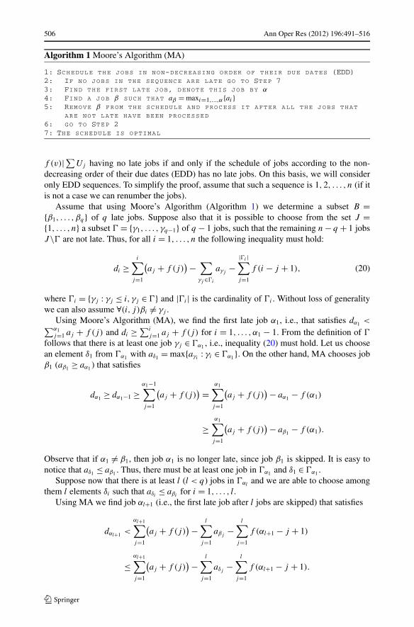
It is well known that the problem 1||∑Uj (with constant job processing times) can besolved optimally by Moore’s Algorithm (Moore 1968). We will prove that this algorithm isstill optimal for the problem 1|pj (v) = aj + f (v)|∑Uj .

Property 3 The problem 1|pj (v) = aj + f (v)|∑Uj can be solved optimally in O(n logn)

steps by Moore’s Algorithm.

Proof The proof will be done using the inductive method in the similar manner as by Sturm(1970). Based on Property 2, we can note that there exists a schedule for 1|pj (v) = aj +

506 Ann Oper Res (2012) 196:491–516

Algorithm 1 Moore’s Algorithm (MA)

1: SCHEDULE THE JOBS IN NON-DECREASING ORDER OF THEIR DUE DATES (EDD)2: IF NO JOBS IN THE SEQUENCE ARE LATE GO TO STEP 73: FIND THE FIRST LATE JOB, DENOTE THIS JOB BY α

4: FIND A JOB β SUCH THAT aβ = maxi=1,...,α{ai }5: REMOVE β FROM THE SCHEDULE AND PROCESS IT AFTER ALL THE JOBS THAT

ARE NOT LATE HAVE BEEN PROCESSED

6: GO TO STEP 27: THE SCHEDULE IS OPTIMAL

f (v)|∑Uj having no late jobs if and only if the schedule of jobs according to the non-decreasing order of their due dates (EDD) has no late jobs. On this basis, we will consideronly EDD sequences. To simplify the proof, assume that such a sequence is 1,2, . . . , n (if itis not a case we can renumber the jobs).

Assume that using Moore’s Algorithm (Algorithm 1) we determine a subset B ={β1, . . . , βq} of q late jobs. Suppose also that it is possible to choose from the set J ={1, . . . , n} a subset � = {γ1, . . . , γq−1} of q − 1 jobs, such that the remaining n − q + 1 jobsJ\� are not late. Thus, for all i = 1, . . . , n the following inequality must hold:

di ≥i∑

j=1

(aj + f (j)

) −∑

γj ∈�i

aγj−

|�i |∑

j=1

f (i − j + 1), (20)

where �i = {γj : γj ≤ i, γj ∈ �} and |�i | is the cardinality of �i . Without loss of generalitywe can also assume ∀(i, j)βi = γj .

Using Moore’s Algorithm (MA), we find the first late job α1, i.e., that satisfies dα1 <∑α1

j=1 aj + f (j) and di ≥ ∑i

j=1 aj + f (j) for i = 1, . . . , α1 − 1. From the definition of �

follows that there is at least one job γj ∈ �α1 , i.e., inequality (20) must hold. Let us choosean element δ1 from �α1 with aδ1 = max{aγi

: γi ∈ �α1}. On the other hand, MA chooses jobβ1 (aβ1 ≥ aα1 ) that satisfies

dα1 ≥ dα1−1 ≥α1−1∑

j=1

(aj + f (j)

) =α1∑

j=1

(aj + f (j)

) − aα1 − f (α1)

≥α1∑

j=1

(aj + f (j)

) − aβ1 − f (α1).

Observe that if α1 = β1, then job α1 is no longer late, since job β1 is skipped. It is easy tonotice that aδ1 ≤ aβ1 . Thus, there must be at least one job in �α1 and δ1 ∈ �α1 .

Suppose now that there is at least l (l < q) jobs in �αland we are able to choose among

them l elements δi such that aδi ≤ aβifor i = 1, . . . , l.

Using MA we find job αl+1 (i.e., the first late job after l jobs are skipped) that satisfies

dαl+1 <

αl+1∑

j=1

(aj + f (j)

) −l∑

j=1

aβj−

l∑

j=1

f (αl+1 − j + 1)

≤αl+1∑

j=1

(aj + f (j)

) −l∑

j=1

aδj −l∑

j=1

f (αl+1 − j + 1).

Ann Oper Res (2012) 196:491–516 507

From (20) follows that there must be at least l + 1 jobs in �αl+1 to satisfy

dαl+1 ≥αl+1∑

j=1

(aj + f (j)

) −∑

γj ∈�αl+1

aγj−

|�αl+1 |∑

j=1

f (αl+1 − j + 1),

and δi ∈ �αl+1 , i = 1, . . . , l. Thus, we find the (l + 1)th element with aδl+1 = max{aγi: γi ∈

�αl+1\{δj }, j = 1, . . . , l}. On the other hand, MA finds βl+1 (i.e., the (l + 1)th late job) withaβl+1 = max{ aβi

: i = 1, . . . , αl+1, i = β1, . . . , βl} and it is easy to notice that aδl+1 ≤ aβl+1 .Therefore, there must be at least l + 1 jobs in �αl+1 and among them l + 1 jobs δi withaδi ≤ aβi

for i = 1, . . . , l + 1. Concluding in the same way, we can show that when MAfinds job αq , then there must be at least q jobs in �αq and it contradicts the assumption|�| = q − 1. Thus MA finds the minimum number of late jobs for the considered schedulingproblem. Note that the complexity of MA is O(n logn) if the algorithm is implemented witha special data structure. �

5 Conclusions

In this paper, we proved that the minimization of the maximum lateness or of the makespanwith release dates is strongly NP-hard even if job processing times are described by simplelinear functions dependent on a number of processed jobs (i.e., a job position in a sequence).Moreover, we showed that the minimization of the makespan with release dates is equiva-lent to the minimization of the maximum lateness if job processing times are described byfunctions dependent on the number of processed jobs and the functions are monotonicallyopposite for these problems.

The main conclusion concerning the proved strong NP-hardness of the considered prob-lems is that the maximum acceptable simplification of job processing time functions (bytheir linearization) does not decrease the complexity of the considered problems. There-fore, it does not decrease the effort required to obtain optimal control decisions but it ratherdecreases their accuracy.

Finally, we also proved that the considered problems with an arbitrary functions describ-ing decrease/increase of a job processing time are polynomially solvable if the functions arethe same for each job. The proper algorithms were provided.

The future research will concern on the analysis of the scheduling problems with posi-tion dependent job processing times under additional constraints and different criteria (e.g.,Leung et al. 2008; Shabtay and Steiner 2008; Steiner and Zhang 2011; Xu et al. 2010).

Acknowledgement This work was financially supported by the Polish Ministry of Science and HigherEducation in years 2012–2013.

Open Access This article is distributed under the terms of the Creative Commons Attribution Licensewhich permits any use, distribution, and reproduction in any medium, provided the original author(s) and thesource are credited.

Appendix

Proof of Lemma 4 The proof will be done using the inductive method. At first observe thatin the optimal schedule the blocks of the enforcer jobs are scheduled according to the EDDrule (Lemma 2) and the sequence of jobs within each block is immaterial (Lemma 1).

508 Ann Oper Res (2012) 196:491–516

Let SEidenote the start time of the first job in the set Ei (for i = 1, . . . ,m). Obviously

if before jobs in E1 any partition job is scheduled, then SE1 > dE1 . Now, we will show thatif more than 3 jobs are scheduled before E2, then all jobs from E2 are late. Assume thatat least 4 partition jobs are scheduled before E2, then based on (11)–(13) and taking intoconsideration that q ∈ X2 and pq(N + 4) > M , we have

CE2 > SE2 > W1 + V (X1) + pq(N + 4) > W1 + V1 − (N + 3)B − 3

4B + pq(N + 4)

= W1 + V1 + W2 + pq(N + 4) − (N + 3)B − 3

4B − W2

> W1 + V1 + W2 + M − (N + 3)B − 3

4B − W2 > W1 + V1 + W2 = dE2 .

Since SE2 > dE2 , then all jobs in E2 are late. Thus, we conclude that in the optimal solutionof DAEL the number of the partition jobs before E2 cannot be greater than 3.

Now we will show that if before E3 more than 6 partition jobs are scheduled, then alljobs in E3 are late. Assume we have at least 7 partition jobs scheduled before the enforcerjobs from E3. From Lemma 3 follows that CE3 is minimal if jobs are scheduled accordingto LPT rule. Thus, CE3 is minimal if the partition jobs are scheduled first. However, fromthe previous considerations follows that the number of the partition jobs before E2 cannotexceed 3 otherwise jobs from E2 are always late. Therefore, jobs are scheduled as follows(E1,X1,E2,X2, q,E3, . . .), where q ∈ X3, then we have

CE3 > SE3 >

2∑

l=1

(Wl + V (Xl)

) + pq

(2(N + 3) + 1

)

>

2∑

l=1

(

Wl + Vl − l(N + 3)B − 3

4B

)

+ W3 + M − W3

>

2∑

l=1

(Wl + Vl) + W3 + M −2∑

l=1

(

l(N + 3)B + 3

4B

)

− W3

>

2∑

l=1

(Wl + Vl) + W3 = dE3 .

Since SE3 > dE3 , then all jobs from E3 are late. Thus, in the optimal solution of DAEL, thenumber of the partition jobs before E3 cannot be greater than 6.

In order to proceed inductively, consider the set Ei . Suppose that before each set El

3(l − 1) partition jobs are scheduled (for l = 1, . . . , i − 1) and before Ei more than 3(i − 1)

jobs are scheduled (i = 2, . . . ,m). On this basis and taking into consideration (11)–(13), wehave

CEi> SEi

>

i−1∑

l=1

(Wl + V (Xl)

) + pq

((i − 1)(N + 3) + 1

)

>

i−1∑

l=1

(Wl + Vl) + Wi + M −i−1∑

l=1

(

l(N + 3)B + 3

4B

)

− WEi

Ann Oper Res (2012) 196:491–516 509

>

i−1∑

l=1

(Wl + Vl) + Wi = dEi,

for i = 2, . . . ,m and q ∈ Xi+1. Thus, we conclude that the number of the partition jobsbefore Ei (for i = 1, . . . ,m) cannot be greater than 3(i − 1) otherwise all jobs in Ei arelate. �

Proof of Lemma 5 From Lemma 3 follows that the completion time of a job is minimalif before it jobs are scheduled according to LPT rule. On the other hand from Lemma 4follows that in the optimal solution the number of the partition jobs before Ei cannot begreater than 3(i − 1) for i = 1, . . . ,m, otherwise all jobs from Ei are late. Under this as-sumption the completion time CXm of the last job in the set Xm is minimal if the schedule ofjobs π∗ is as follows: (E1,X1,E2,X2,E3, . . . ,Ei,Xi,Ei+1, . . . ,Xm−1,Em,Xm). Thus, thecompletion time of the last job in Xm for π∗ is equal to:

CXm

(π∗) =

m∑

l=1

(Wl + V (Xl)

).

Now we will show that the optimal schedule is in the form of π∗. To prove it we will usethe inductive principle.

Obviously before E1 no partition jobs are scheduled. First assume that before an enforcerjob from E2 at last 2 partition jobs are scheduled (i.e., E1,1,2, eN+1,3, eN+2, . . . , e2N, . . .).Note that jobs from Ei are indistinguishable (i = 1, . . . ,m). Observe that in this case thevalue V (X1) (where X1 = {1,2,3}) increases by a3 and W2 (where E2 = {eN+1, eN+2, . . . ,

e2N }) decreases by aE . On this basis and taking into consideration (11) and (13), the com-pletion time of the last job in E2 can be estimated as follows:

CE2 > W1 + V (X1) + a3 + W2 − aE

> W1 + V1 + W2 + M − (N + 3)B − 3

4B − N

> W1 + V1 + W2 = dE2 .

Since CE2 > dE2 , then the last scheduled job in E2 is late. Observe that this value is greaterif more enforcer jobs from E2 are moved before job 3. Thus, E2 is not late if jobs from E2

are scheduled one after another, i.e., (E1,1,2,E2,3, . . .). However, if before E2 at last 2partition jobs are scheduled, then CXm can be estimated as follows:

CXm > CXm

(π∗) + a3 − NaE

>

m∑

l=1

(Wl + Vl) + M −m∑

l=1

(

l(N + 3)B + 3

4B

)

− N

>

m∑

l=1

(Wl + Vl) = D.

Since CXm > D, then Lmax > 0. Taking it into consideration and based on Lemma 4, weconclude that in the optimal solution jobs from E2 are processed one after another and 3partition jobs are scheduled between E1 and E2, otherwise Lmax > 0.

510 Ann Oper Res (2012) 196:491–516

Now we will show that if before E3 less than 6 partition jobs are scheduled, thenLmax > 0. Assume we have at last 5 partition jobs scheduled before an enforcer job fromE3. First we will show that in the optimal solution of DAEL jobs from E3 have to be pro-cessed one after another. From the previous considerations follows that the schedule is givenas follows: (E1,X1,E2,4,5, e2N+1,6, e2N+2, . . . , e3N, . . .). Thus, the completion time of thelast job in E3 is equal to:

CE3 =2∑

l=1

(Wl + V (Xl)

) + a6 + W2 − aE

>

2∑

l=1

(Wl + Vl) + W3 + M −2∑

l=1

(

l(N + 3)B + 3

4B

)

− N

>

2∑

l=1

(Wl + Vl) + W3 = dE3 .

Since CE3 > dE3 , then the last scheduled job in E3 is late. Observe that this value is greaterif more enforcer jobs from E3 are moved before job 6. Thus, E3 is not late if jobs from E3

are scheduled one after another, i.e., (E1,X1,E2,4,5,E3,6, . . .). However, if before E3 atlast 5 jobs are scheduled, then CXm can be estimated as follows:

CXm > CXm

(π∗) + a6 − NaE

>

m∑

l=1

(Vl + Wl) + M −m∑

l=1

(

l(N + 3)B + 3

4B

)

− N

>

m∑

l=1

(Vl + Wl) = D.

Taking it into consideration and based on Lemma 4, we conclude that in the optimal solutionjobs from E3 are processed one after another and 3 partition jobs are scheduled between E2

and E3, otherwise Lmax > 0.In order to proceed inductively consider the set Ei . Suppose that between El and

El+1 exactly 3 partition jobs are scheduled (l = 1, . . . , i − 2). Assume that before Ei

at last 3(i − 1) − 1 partition jobs are scheduled. From the previous considerations fol-lows that the schedule is given as follows: (E1,X1,E2,X2,E3, . . . ,Ei−1,3(i − 1) −2,3(i − 1) − 1, eiN+1,3(i − 1), eiN+2, . . . , e(i+1)N , . . .). On this basis and taking into con-sideration (11) and (13), the completion time of the last job in Ei can be estimated as fol-lows:

CEi>

i−1∑

l=1

(Wl + V (Xl)

) + a3(i−1) + Wi − NaE

>

i−1∑

l=1

(Wl + Vl) + Wi + M −i−1∑

l=1

(

l(N + 3)B + 3

4B

)

− N

>

i−1∑

l=1

(Wl + Vl) + Wi = dEi,

Ann Oper Res (2012) 196:491–516 511

for i = 2, . . . ,m. Thus, jobs from Ei must be scheduled one after another, i.e., (E1,X1, . . . ,

Ei−1,3(i − 1) − 2,3(i − 1) − 1,Ei,3(i − 1), . . .), otherwise the last job in Ei is late (fori = 1, . . . ,m). However, if before Ei at last 3(i − 1) jobs are scheduled, then CXm can beestimated as follows:

CXm > CXm

(π∗) + a3(i−1) − NaE

>

m∑

l=1

(Vl + Wl) + M −m∑

l=1

(

l(N + 3)B + 3

4B

)

− N

>

m∑

l=1

(Vl + Wl) = D.

for i = 1, . . . ,m − 1.Thus, we conclude that in the optimal solution jobs from the set Ei are scheduled

one after another and between Ei and Ei+1 exactly 3 partition jobs are scheduled (fori = 1, . . . ,m − 1), otherwise Lmax > 0. �

Proof of Lemma 9 The proof will be done using the inductive method in the similar manneras the proof of Lemma 4.

At first observe that in the optimal schedule the blocks of the enforcer jobs are scheduledaccording to the EDD rule (Lemma 7) and the sequence of jobs within each block is immate-rial (Lemma 6). Note also that CEi

is minimal if before Ei partition jobs are scheduled first,since bj < bE for j = 1, . . . ,3m and i = 1, . . . ,m (Lemma 8). However, the sum of pro-cessing times of the enforcer jobs Ei for an arbitrary schedule π (denoted as W ′

i ) is alwaysgreater than the sum of processing times of the enforcer jobs Ei for schedule π∗ (denotedas Wi ) decreased by bEmN(N + 3), i.e., W ′

i > Wi − bEmN(N + 3) for i = 1, . . . ,m. Notethat m(N + 3) is the maximum possible position in a schedule for DLEL.

Assume that before E1 at least one partition job is scheduled. Thus, based on (19), thecompletion time of the last job in E1 can be estimated as follows:

CE1 > pq(1) + W1 − mN(N + 3)bE > W1 + a − M − mN(N + 3)bE > W1 = dE1 .

Therefore, we conclude that in the optimal solution of DLEL any partition job can be sched-uled before E1, otherwise Lmax > 0.

Now, we will show that if more than 3 jobs are scheduled before E2, then the last jobfrom E2 is late. Assume that at least 4 partition jobs are scheduled before E2. Based on (17)and (19), we have

CE2 > W1 + V (X1) + pq(N + 4) + W2 − mN(N + 3)bE

> W1 + V1 − (N + 3)B − 3

4B + W2 + a − M(N + 4) − mN(N + 3)bE

> W1 + V1 + W2 + a − M(N + 4) − mN(N + 3)bE − (N + 3)B − 3

4B

> W1 + V1 + W2 = dE2 ,

where q ∈ X2. Since CE2 > dE2 , then the last job in E2 is late. Thus, we conclude that inthe optimal solution of DLEL the number of the partition jobs before E2 cannot be greaterthan 3.

512 Ann Oper Res (2012) 196:491–516

Now we will show that if before E3 more than 6 partition jobs are scheduled, then alljobs in E3 are late. Assume we have at least 7 partition jobs scheduled before the enforcerjobs from E3. From Lemma 8 follows that CE3 is minimal if the partition jobs are scheduledfirst. However, from the previous considerations follows that the number of the partition jobsbefore E2 cannot exceed 3 otherwise Lmax > 0. Therefore, jobs are scheduled as follows(E1,X1,E2,X2, q,E3, . . .) (where q ∈ X3 = {7,8,9}) and we have

CE3 >

2∑

l=1

(Wl + V (Xl)

) + pq

(2(N + 3) + 1

) + W3 − mN(N + 3)bE

>

2∑

l=1

(Wl + Vl) + W3 + a − M(2(N + 3) + 1

) − mN(N + 3)bE

−2∑

l=1

(

l(N + 3)B + 3

4B

)

>

2∑

l=1

(Wl + Vl) + W3 = dE3 ,

Thus, in the optimal solution of DAEL, the number of the partition jobs before E3 cannotbe greater than 6.

In order to proceed inductively, consider the set Ei . Suppose that before each set El

3(l − 1) partition jobs are scheduled (for l = 1, . . . , i − 1) and before Ei more than 3(i − 1)

jobs are scheduled (i = 2, . . . ,m). On this basis and taking into consideration (17) and (19),we have

CEi>

i−1∑

l=1

(Wl + V (Xl)

) + pq

((i − 1)(N + 3) + 1

) + Wi − mN(N + 3)bE

>

i−1∑

l=1

(Wl + Vl) + Wi + a − M((i − 1)(N + 3) + 1

) − mN(N + 3)bE

−i−1∑

l=1

(

l(N + 3)B + 3

4B

)

>

i−1∑

l=1

(Wl + Vl) + Wi = dEi,

for i = 2, . . . ,m and q ∈ Xi . Thus, we conclude that the number of the partition jobs beforeEi (for i = 1, . . . ,m) cannot be greater than 3(i − 1) otherwise all jobs in Ei are late. �

Proof of Lemma 10 The proof will be done in the similar manner as the proof of Lemma 5.From Lemma 8 follows the completion time of a job is minimal if jobs before it are

scheduled according to the non-decreasing order of bj . On the other hand from Lemma 9follows that in the optimal solution the number of the partition jobs before Ei cannot begreater than 3(i − 1) for i = 1, . . . ,m, otherwise at last one job in Ei is late. Under thisassumption the completion time CXm of the last job in the set Xm is minimal if the scheduleof jobs π∗ is as follows: (E1,X1,E2,X2,E3, . . . ,Ei,Xi,Ei+1, . . . ,Xm−1,Em,Xm). Thus,the completion time of the last job in Xm for π∗ is equal to:

CXm

(π∗) =

m∑

i=1

(Wl + V (Xl)

).

Now we will show that the optimal schedule is in the form of π∗. To prove it we will usethe inductive principle.

Ann Oper Res (2012) 196:491–516 513

From Lemma 9 follows that before E1 no partition jobs are scheduled. First as-sume that before an enforcer job from E2 at last 2 partition jobs are scheduled (i.e.,E1,1,2, eN+1,3, eN+2, . . . , e2N, . . .). Note that jobs from Ei are indistinguishable (i =1, . . . ,m). Observe that in this case the value V (X1) decreases by b3 (q ∈ X1 = {1,2,3})and W2 increases by bE , where E2 = {eN+1, eN+2, . . . , e2N }. On this basis and taking intoconsideration (17)–(19), the completion time of the last job in E2 can be estimated as fol-lows:

CE2 = W1 + V (X1) − b3 + W2 + bE

> W1 + V1 + W2 + MN − (N + 3)B − 3

4B

> W1 + V1 + W2 = dE2 .

Since CE2 > dE2 , then the last scheduled job in E2 is late. Observe that CE2 is greater ifmore enforcer jobs from E2 are moved before job 3. Thus knowing that V (Xi) < Vi +i(N + 3)B , any job from E2 is not late if jobs from E2 are scheduled one after another, i.e.,(E1,1,2,E2,3, . . .):

CE2 = W1 + V (X1) − (a − (N + 3)b3

) + W2 + NbE

< W1 + V1 + (N + 3)B − a + (N + 3)b3 + W2 + NbE

= dE − a + (N + 3)bE < dE2 .

However, if before E2 at last 2 partition jobs are scheduled, then CXm can be estimated asfollows:

CXm = CXm

(π∗) − Nb3 + NbE

>

m∑

l=1

(Wl + Vl) + MN2 −m∑

l=1

(

l(N + 3)B + 3

4B

)

>

m∑

l=1

(Wl + Vl) = D.

Since CXm > D, then Lmax > 0. Taking it into consideration and based on Lemma 9, weconclude that in the optimal solution jobs from E2 are processed one after another and 3partition jobs are scheduled between E1 and E2, otherwise Lmax > 0.

Now we will show that if before E3 less than 6 partition jobs are scheduled, thenLmax > 0. Assume we have at last 5 partition jobs scheduled before an enforcer job fromE3. First we will show that in the optimal solution of DLEL jobs from E3 have to be pro-cessed one after another. From the previous considerations follows that the schedule is givenas follows: (E1,X1,E2,4,5, e2N+1,6, e2N+2, . . . , e3N, . . .). Thus, the completion time of thelast job in E3 can be estimated as follows:

CE3 =2∑

l=1

(Wl + V (Xl)

) − b6 + W3 + bE

>

2∑

l=1

(Wl + Vl) + W3 + MN −2∑

l=1

(

l(N + 3)B + 3

4B

)

> dE3 .

514 Ann Oper Res (2012) 196:491–516

Since CE3 > dE3 , then the last scheduled job in E3 is late. Observe that this value is greaterif more enforcer jobs from E3 are moved before job 6. Thus, E3 is not late if jobs from E3

are scheduled one after another, i.e., (E1,X1,E2,4,5,E3,6, . . .). However, if before E3 atlast 5 jobs are scheduled, then CXm can be estimated as follows:

CXm = CXm

(π∗) − Nb6 + NbE

>

m∑

l=1

(Vl + Wl) + MN2 −m∑

l=1

(

l(N + 3)B + 3

4B

)

>

m∑

l=1

(Vl + Wl) = D.

Taking it into consideration and based on Lemma 9, we conclude that in the optimal solutionjobs from E3 are processed one after another and 3 partition jobs are scheduled between E2

and E3, otherwise Lmax > 0.In order to proceed inductively consider the set Ei . Suppose that between El and El+1 ex-

actly 3 partition jobs are scheduled (l = 1, . . . , i−2). Assume that before Ei at last 3(i−1)−1 partition jobs are scheduled. From the previous considerations follows that the schedule isgiven as follows: (E1,X1,E2,X2,E3, . . . ,Ei−1,3(i − 1) − 2,3(i − 1) − 1, eiN+1,3(i − 1),

eiN+2, . . . , e(i+1)N , . . .). On this basis and taking into consideration (17)–(19), the comple-tion time of the last job in Ei can be estimated as follows:

CEi=

i−1∑

l=1

(Wl + V (Xl)

) − b3(i−1) + Wi + bE

>

i−1∑

l=1

(Wl + Vl) + Wi + MN −i−1∑

l=1

(

l(N + 3)B + 3

4B

)

> dEi,

for i = 2, . . . ,m. Thus, jobs from Ei must be scheduled one after another, i.e., (E1,X1, . . . ,

Ei−1,3(i − 1) − 2,3(i − 1) − 1,Ei,3(i − 1), . . .), otherwise the last job in Ei is late (fori = 1, . . . ,m). However, if before Ei at last 3(i − 1) jobs are scheduled, then CXm can beestimated as follows:

CXm = CXm

(π∗) − Nb3(i−1) + NbE

>

m∑

l=1

(Vl + Wl) + MN2 −m∑

l=1

(

l(N + 3)B + 3

4B

)

> D,

for i = 1, . . . ,m − 1.Thus, we conclude that in the optimal solution jobs from the set Ei are scheduled

one after another and between Ei and Ei+1 exactly 3 partition jobs are scheduled (fori = 1, . . . ,m − 1), otherwise Lmax > 0. �

References

Adler, P. S., & Clark, K. B. (1991). Behind the learning curve: a sketch of the learning process. ManagementScience, 37, 267–281.

Ann Oper Res (2012) 196:491–516 515

Arimoto, S., Kawamura, S., & Miyazaki, F. (1984). Bettering operations of robots by learning. Journal ofRobotic Systems, 1, 123–140.

Bachman, A., & Janiak, A. (2004). Scheduling jobs with position dependent processing times. The Journalof the Operational Research Society, 55, 257–264.

Biskup, D. (1999). Single-machine scheduling with learning considerations. European Journal of Opera-tional Research, 115, 173–178.

Biskup, D. (2008). A state-of-the-art review on scheduling with learning effects. European Journal of Oper-ational Research, 188, 315–329.

Busoniu, L., Babuška, R., & De Schutter, B. (2008). A comprehensive survey of multiagent reinforcementlearning. IEEE Transactions on Systems, Man and Cybernetics. Part C, Applications and Reviews, 38,156–172.

Carlson, J. G., & Rowe, R. G. (1976). How much does forgetting cost? Industrial Engineering, 8, 40–47.Cheng, T. C. E., Ding, Q., & Lin, B. M. T. (2004). A concise survey of scheduling with time-dependent

processing times. European Journal of Operational Research, 152, 1–13.Cheng, T. C. E., Lee, W.-C., & Wu, C.-C. (2010). Single-machine scheduling with deteriorating functions for

job processing times. Applied Mathematical Modelling, 34, 4171–4178.Cheng, T. C. E., & Wang, G. (2000). Single machine scheduling with learning effect considerations. Annals

of Operations Research, 98, 273–290.Cheng, T. C. E., Wu, C.-C., & Lee, W.-C. (2008). Some scheduling problems with deteriorating jobs and

learning effects. Computers & Industrial Engineering, 54, 972–982.Cochran, E. B. (1960). New concepts of the learning curve. The Journal of Industrial Engineering, 11, 317–

327.Dababneh, A. J., Swanson, N., & Shell, R. L. (2001). Impact of added rest breaks on the productivity and

well being of workers. Ergonomics, 44, 164–174.Eilon, S. (1964). On a mechanistic approach to fatigue and rest periods. International Journal of Production

Research, 3, 327–332.Garey, M. R., & Johnson, D. S. (1979). Computers and intractability: a guide to the theory of NP-

completeness. San Francisco: Freeman.Gawiejnowicz, S. (1996). A note on scheduling on a single processor with speed dependent on a number of

executed jobs. Information Processing Letters, 57, 297–300.Gawiejnowicz, S. (2008). Time-dependent scheduling. Berlin: Springer.Graham, R. L., Lawler, E. L., Lenstra, J. K., & RinnooyKan, A. H. G. (1979). Optimization and approxima-

tion in deterministic sequencing and scheduling: a survey. Annals of Discrete Mathematics, 5, 287–326.Holzer, H. P., & Riahi-Belkaoui, A. (1986). The learning curve: a management accounting tool. Westport:

Quorum Books.Jaber, Y. M., & Bonney, M. (1999). The economic manufacture/order quantity (EMQ/EOQ) and the learning

curve: Past, present, and future. International Journal of Production Economics, 59, 93–102.Janiak, A., & Rudek, R. (2010). Scheduling jobs under an aging effect. The Journal of the Operational

Research Society, 61, 1041–1048.Janiak, A., & Rudek, R. (2011). A note on the learning effect in multi-agent optimization. Expert Systems

With Applications, 38, 5974–5980.Keachie, E. C., & Fontana, R. J. (1966). Production lot sizing under a learning effect. Management Science,

13, 102–108.Kerzner, H. (1998). Project management: a system approach to planning, scheduling, and controlling. New

York: Wiley.Kuo, W.-H., & Yang, D.-L. (2008). Minimizing the makespan in a single-machine scheduling problem with

the cyclic process of an aging effect. The Journal of the Operational Research Society, 59, 416–420.Lee, W.-C., & Lai, P.-J. (2011). Scheduling problems with general effects of deterioration and learning.

Information Sciences, 181, 1164–1170.Lee, W.-C., Wu, C.-C., & Hsu, P.-H. (2010). A single-machine learning effect scheduling problem with

release times. Omega, 38, 3–11.Leung, J. Y.-T., Li, H., & Pinedo, M. (2008). Scheduling orders on either dedicated or flexible machines in

parallel to minimize total weighted completion time. Annals of Operations Research, 159, 107–123.Li, C.-L., & Cheng, T. C. E. (1994). An economic production quantity model with learning and forgetting

considerations. Production and Operations Management, 3, 118–132.Lien, T. K., & Rasch, F. O. (2001). Hybrid automatic-manual assembly systems. Annals of the CIRP, 50,

21–24.Mandich, N. V. (2003). Overview of surface preparation of metals prior to finishing: Part 2. Metal Finishing,

101, 33–58.Moore, J. M. (1968). An n jobs, one machine sequencing algorithm for minimizing the number of late jobs.

Management Science, 15, 102–109.

516 Ann Oper Res (2012) 196:491–516

Mosheiov, G. (2001). Parallel machine scheduling with a learning effect. The Journal of the OperationalResearch Society, 52, 1–5.

Roberts, P. (1983). A theory of the learning process. The Journal of the Operational Research Society, 34,71–79.

Rudek, A., & Rudek, R. (2011). A note on optimization in deteriorating systems using scheduling problemswith the aging effect and resource allocation models. Computers & Mathematics With Applications, 62,1870–1878.

Shabtay, D., & Steiner, G. (2008). The single-machine earliness-tardiness scheduling problem with due dateassignment and resource-dependent processing times. Annals of Operations Research, 159, 25–40.

Steiner, G., & Zhang, R. (2011). Minimizing the weighted number of tardy jobs with due date assignmentand capacity-constrained deliveries. Annals of Operations Research, 191, 171–181.

Stanford, M., & Lister, P. M. (2004). Investigation into the relationship between tool-wear and cutting envi-ronments when turning EN32 steel. Industrial Lubrication and Tribology, 56, 114–121.

Sturm, L. B. J. M. (1970). A simple optimality proof of Moore’s sequencing algorithm. Management Science,17, 116–118.

Wang, J.-B., & Wang, M.-Z. (2011). Worst-case behavior of simple sequencing rules in flow shop schedulingwith general position-dependent learning effects. Annals of Operations Research. 191, 155–169.

Webb, G. K. (1994). Integrated circuit (IC) pricing. High Technology Management Research, 5, 247–260.Whiteson, S., & Stone, P. (2004). Adaptive job routing and scheduling. Engineering Applications of Artificial

Intelligence, 17, 855–869.Wright, T. P. (1936). Factors affecting the cost of airplanes. Journal of the Aeronautical Sciences, 3, 122–128.Wu, C.-C., Lee, W.-C., & Chen, T. (2007). Heuristic algorithms for solving the maximum lateness scheduling

problem with learning considerations. Computers & Industrial Engineering, 52, 124–132.Xu, K., Feng, Z., & Ke, L. (2010). A branch and bound algorithm for scheduling jobs with controllable

processing times on a single machine to meet due dates. Annals of Operations Research, 181, 303–324.Yang, D.-L., & Kuo, W.-H. (2009). Single-machine scheduling with both deterioration and learning effects.

Annals of Operations Research, 172, 315–327.Yang, S.-J., & Yang, D.-L. (2010). Minimizing the makespan on single-machine scheduling with aging effect

and variable maintenance activities. Omega, 38, 528–533.Yang, S.-J., Yang, D.-L., & Cheng, T. C. E. (2010). Single-machine due-window assignment and scheduling

with job-dependent aging effects and deteriorating maintenance. Computers & Operations Research,37, 1510–1514.

Yelle, L. E. (1979). The learning curve: historical review and comprehensive study. Decision Sciences, 10,302–328.

Zhang, X., Yan, G., Huang, W., & Tang, G. (2011). Single-machine scheduling problems with time andposition dependent processing times. Annals of Operations Research, 186, 345–356.