Scheduling sports competitions at multiple venues—Revisited

European Journal of Operational Research 175 (2006) 171–186

www.elsevier.com/locate/ejor

Discrete Optimization

Scheduling sports competitions at multiple venues—Revisited

A. Lim a, B. Rodrigues b,*, X. Zhang a

a Department of IEEM, Hong Kong University of Science and Technology, Clearwater Bay, Kowloon, Hong Kongb School of Business, Singapore Management University, 469 Bukit Timah Road, Singapore 259756, Singapore

Received 11 September 2003; accepted 16 March 2005Available online 23 June 2005

Abstract

In this work, we study scheduling sports competitions at multiple venues, a problem recently introduced by Urbanand Russell [T.L. Urban, R.A. Russell, Scheduling sports competitions on multiple venues, European Journal of Oper-ational Research 148 (2003) 302–311]. The distinguishing feature of the problem is that venues come into play whenscheduling. We develop beam search and simulated annealing approaches to the problem and its extension. Computa-tional experiments were conducted and algorithms compared and analyzed. We found that the simulated annealingalgorithm with specialized neighborhood moves achieved superior solutions in significantly shorter times than themethod of Urban and Russell.� 2005 Elsevier B.V. All rights reserved.

Keywords: Scheduling; Sports management; Beam search; Meta-heuristic

1. Introduction

Sports competition scheduling has attractedmuch interest among researchers. In a number ofstudies, including Ball and Webster [3], De Werra,Jacot-Descombes and Masson [17], Russell andLeung [15], Nemhauser and Trick [12] and Henz[6], each team to be scheduled is assumed to have

0377-2217/$ - see front matter � 2005 Elsevier B.V. All rights reservdoi:10.1016/j.ejor.2005.03.029

* Corresponding author. Fax: +65 68220777.E-mail address: [email protected] (B. Rodrigues).

its own competition venue. Recently, motivatedby the request from a head coach of a major col-lege football team to have teams participate at ven-ues twice and compete against each other at leastonce, where any two teams should not competetwice at the same venue and where all teams com-pete at all times, Urban and Russell [16] proposeda multi-venue problem where ‘‘venue comes intoplay as part of the scheduling process’’.

In Urban and Russell�s model, given N (i =1, 2, . . . , N, N is even) teams, T(t = 1, 2, . . . , T) peri-ods of time and S(s = 1, 2, . . . , S) venues, whereN = T = 2S, N/2 competitions are played ineach period and each competition takes place at a

ed.

mailto:[email protected]

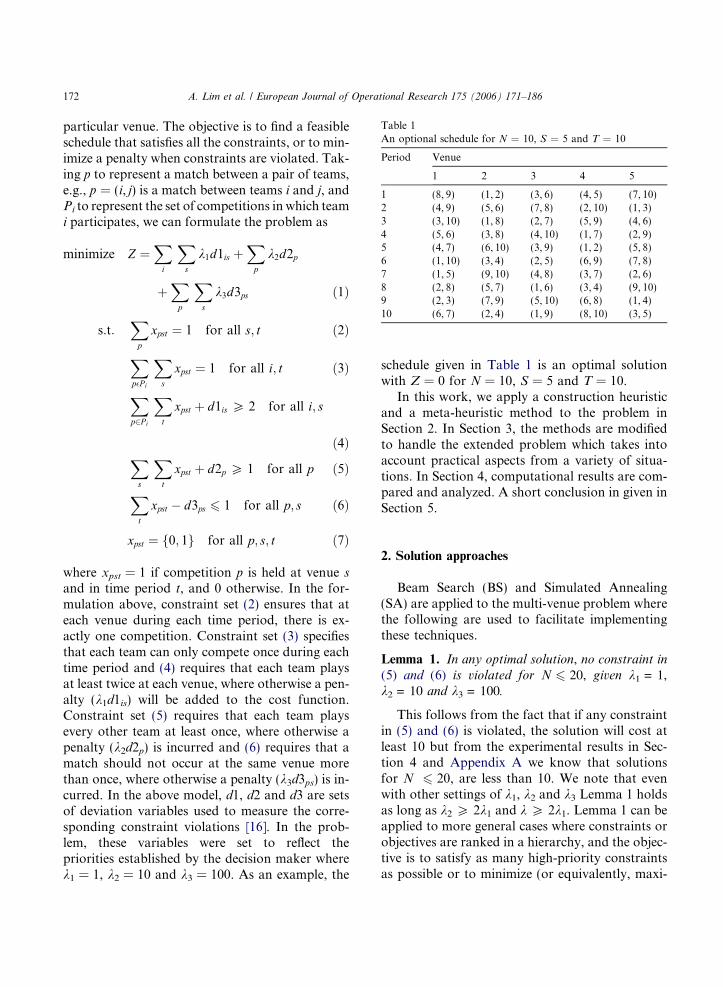
Table 1An optional schedule for N = 10, S = 5 and T = 10

Period Venue

1 2 3 4 5

1 (8, 9) (1, 2) (3, 6) (4, 5) (7, 10)2 (4, 9) (5, 6) (7, 8) (2, 10) (1, 3)3 (3, 10) (1, 8) (2, 7) (5, 9) (4, 6)4 (5, 6) (3, 8) (4, 10) (1, 7) (2, 9)5 (4, 7) (6, 10) (3, 9) (1, 2) (5, 8)6 (1, 10) (3, 4) (2, 5) (6, 9) (7, 8)7 (1, 5) (9, 10) (4, 8) (3, 7) (2, 6)8 (2, 8) (5, 7) (1, 6) (3, 4) (9, 10)9 (2, 3) (7, 9) (5, 10) (6, 8) (1, 4)10 (6, 7) (2, 4) (1, 9) (8, 10) (3, 5)

172 A. Lim et al. / European Journal of Operational Research 175 (2006) 171–186

particular venue. The objective is to find a feasibleschedule that satisfies all the constraints, or to min-imize a penalty when constraints are violated. Tak-ing p to represent a match between a pair of teams,e.g., p = (i, j) is a match between teams i and j, andPi to represent the set of competitions in which teami participates, we can formulate the problem as

minimize Z ¼X

i

Xs

k1d1is þX

p

k2d2p

þX

p

Xs

k3d3ps ð1Þ

s:t:X

p

xpst ¼ 1 for all s; t ð2Þ

Xp�P i

Xs

xpst ¼ 1 for all i; t ð3Þ

Xp2P i

Xt

xpst þ d1is P 2 for all i; s

ð4ÞX

s

Xt

xpst þ d2p P 1 for all p ð5Þ

Xt

xpst � d3ps 6 1 for all p; s ð6Þ

xpst ¼ f0; 1g for all p; s; t ð7Þ

where xpst = 1 if competition p is held at venue sand in time period t, and 0 otherwise. In the for-mulation above, constraint set (2) ensures that ateach venue during each time period, there is ex-actly one competition. Constraint set (3) specifiesthat each team can only compete once during eachtime period and (4) requires that each team playsat least twice at each venue, where otherwise a pen-alty (k1d1is) will be added to the cost function.Constraint set (5) requires that each team playsevery other team at least once, where otherwise apenalty (k2d2p) is incurred and (6) requires that amatch should not occur at the same venue morethan once, where otherwise a penalty (k3d3ps) is in-curred. In the above model, d1, d2 and d3 are setsof deviation variables used to measure the corre-sponding constraint violations [16]. In the prob-lem, these variables were set to reflect thepriorities established by the decision maker wherek1 = 1, k2 = 10 and k3 = 100. As an example, the

schedule given in Table 1 is an optimal solutionwith Z = 0 for N = 10, S = 5 and T = 10.

In this work, we apply a construction heuristicand a meta-heuristic method to the problem inSection 2. In Section 3, the methods are modifiedto handle the extended problem which takes intoaccount practical aspects from a variety of situa-tions. In Section 4, computational results are com-pared and analyzed. A short conclusion in given inSection 5.

2. Solution approaches

Beam Search (BS) and Simulated Annealing(SA) are applied to the multi-venue problem wherethe following are used to facilitate implementingthese techniques.

Lemma 1. In any optimal solution, no constraint in

(5) and (6) is violated for N 6 20, given k1 = 1,k2 = 10 and k3 = 100.

This follows from the fact that if any constraintin (5) and (6) is violated, the solution will cost atleast 10 but from the experimental results in Sec-tion 4 and Appendix A we know that solutionsfor N 6 20, are less than 10. We note that evenwith other settings of k1, k2 and k3 Lemma 1 holdsas long as k2 P 2k1 and k P 2k1. Lemma 1 can beapplied to more general cases where constraints orobjectives are ranked in a hierarchy, and the objec-tive is to satisfy as many high-priority constraintsas possible or to minimize (or equivalently, maxi-

A. Lim et al. / European Journal of Operational Research 175 (2006) 171–186 173

mize) high-priority objectives first. Thus, Lemma 1can be used if the primary objective is to minimizethe number of violated constraints in set (6), whilethe secondary objective is to minimize the numberof violated constraints in set (5), and lastly to min-imize those violated in set (4). This is the underlin-ing reason why penalty coefficients were set to bek1 = 1, k2 = 10 and k3 = 100.

From Lemma 1, it is easy to derive the follow-ing lemmas:

Lemma 2. In any optimal solution, all competitions

(i, j) with i < j occur once in the solution, and the

remaining N/2 competitions are in {(i, i + 1)ji is odd,

1 6 i 6 N}.

Lemma 3. There exists an optimal solution such

that the competition played at Venue 1 in Period 1is p = (1, 2) where competitions played at Venues 1

to S in Period 1 can be sorted in lexicographic order.

Lemma 4. There exists an optimal solution with the

following property: competitions in the first period

are generated from one of 2S�2 sequences by

exchanging 2x with 2x + l(2 6 x 6 S � 1) from

the original sequence (1, 2, 3, 4, 5, . . . , N � 2, N �1, N).

Lemma 3 is derived by swapping competitionsbetween two periods or two venues. Lemma 4 re-sults from Lemma 3 and renumbering takingadvantage of symmetries between teams. WithLemma 4, the possible choices of competitionsfor Period 1 are reduced from N!/2S to 2S�2. Forthe case N = 6, the reduction is from 90 = 720/8to 2 = 23�2. The two sequences are (1, 2, 3, 4, 5, 6)and (1, 2, 3, 5, 4, 6), which correspond to the twoschedules {(1, 2), (3, 4), (5, 6)} and {(1, 2), (3, 5),(4, 6)}, respectively.

2.1. Using beam search

BS [11,14] expands only the p most promisingnodes at each depth level of Breadth First Search(BFS) and thus avoids the combinatorial explosionproblem of BFS. For the multi-venue problem,each of the T · S games Gt,s ordered by the periodnumber t and, in case of ties, the venue number s,corresponds to a depth level of BS. Initially, the

beam search procedure assigns (1, 2) to the firstgame G1,1, i.e. the competition at Venue 1 duringPeriod 1, and thus generates the initial parent.For every subsequent step, the procedure expandsat most b children from each parent of the previ-ous step. At this time, the b children are simplythose matches with the smallest local evaluationcost, L = hv, �f, sdi, in the lexicographic order.

In the definition of L, m is the objective value ofthe partial schedule, i.e. the penalties specified bythe problem definition. However, with only thevalue of m the algorithm is unable to distinguishmore promising child nodes, especially in earlystages of the BS procedure when most nodes havea m value of 0. Hence, f and sd are used to furtherdifferentiate nodes. For each venue s, fs is the differ-ence between the number of competitions that maytake place at s in future time periods and the num-ber of required competitions at s. For example, ifcompetitions {(1, 3), (2, 4), (3, 4)} are allowed totake place at Venue 1 and one more competitionis required at Venue 1, f1 is thus 2 (i.e. 3 � 1).The overall f of the partial schedule is then takento be the smallest fs for all s (1 6 s 6 S). Next, letvisiti,s denote the number of times team i has playedat venue s, and let remaini,s = max(2 � visiti,s, 0).For each venue s, sds is the standard deviation ofremaini,s for all i (1 6 i 6 N). The overall standarddeviation, sd, of the partial schedule is then definedas sum of sds for all s.

The rationale behind using �f in L is to maxi-mize possible choices of future competitions ateach venue, and thus to increase the chance offinding better complete schedules. Meanwhile,the aim in using sd is to distribute teams moreevenly among venues so that final schedules aremore balanced. In addition, the L of a child nodecan be efficiently computed from its parent nodewith a time complexity of O(N).

The at most p · b children of the current step, de-noted as the cth step, are then sorted according totheir overall evaluation cost, O, and only the best p

are retained which, in turn, serve as parent nodesin the (c + 1)th step. In view of the tight constraintsof the multi-venue problem, a look-ahead procedureis necessary both to ensure the feasibility of resultingsolutions and to improve their quality. More pre-cisely, when calculating the overall evaluation cost

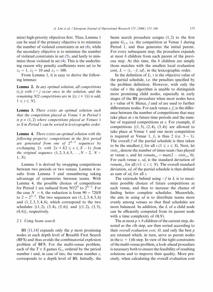
Step 5(1,2) (3,4) (5,6) (7,8)(7,8)

(1,2) (3,4) (5,6) (7,8)(7,8) (5,6)

(1,2) (3,4) (5,6) (7,8)(7,8) (1,2)

Step 1(1,2)

(1,2) (3,4) (5,6) (7,8)(6,8)

Step 6

Fig. 2. The beam search tree.


of an expanded child, the procedure greedily con-structs at most d more games forward from the cthstep. The overall evaluation cost O is a function ofL�s at the cth and (c + d)th-depth levels, denotedLc and Lc+d, respectively. A simple way to calculateO is by the formula O = w1 · Lc + w2 · Lc+d

where w1 + w2 = 1. The underlining rationale is totake into account estimated future costs of currentchoices, instead of depending entirely on the Lc atthe current depth. In our experiments, the para-meters p, b, d, w1 and w2 were set as 2000, 10, 5, 0.5and 0.5, respectively.

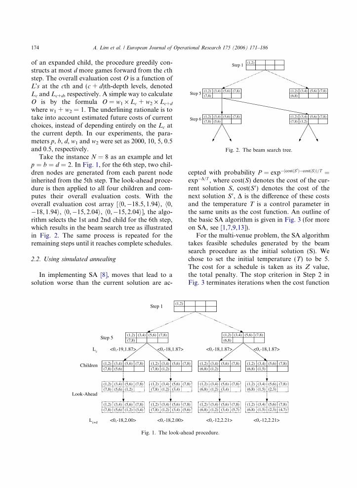
Take the instance N = 8 as an example and letp = b = d = 2. In Fig. 1, for the 6th step, two chil-dren nodes are generated from each parent nodeinherited from the 5th step. The look-ahead proce-dure is then applied to all four children and com-putes their overall evaluation costs. With theoverall evaluation cost array [h0,�18.5, 1.94i, h0,�18, 1.94i, h0,�15, 2.04i, h0,�15, 2.04i], the algo-rithm selects the 1st and 2nd child for the 6th step,which results in the beam search tree as illustratedin Fig. 2. The same process is repeated for theremaining steps until it reaches complete schedules.

2.2. Using simulated annealing

In implementing SA [8], moves that lead to asolution worse than the current solution are ac-

Children

Step 5

<0,-18,2.00>Lc+d

Look-Ahead

(1,2) (3,4) (5,6) (7,8)(7,8)

(1,2) (3,4) (5,6) (7,8)(7,8) (5,6)

(1,2) (3,4) (5,6) (7,(7,8) (1,2)

(1,2) (3,4) (5,6) (7,8)(7,8) (5,6) (1,2)

(1,2) (3,4) (5,6) (7,(7,8) (1,2) (3,4)

(1,2) (3,4) (5,6) (7,8)(7,8) (5,6) (1,2) (3,4)

(1,2) (3,4) (5,6) (7,(7,8) (1,2) (3,4) (5,

Step 1(1,2)

<0,-18,2.00>

<0,-19,1.87>Lc <0,-18,1.87>

Fig. 1. The look-ahe

cepted with probability P ¼ exp�ðcostðS0Þ�costðSÞÞ=T ¼exp�D=T , where cost(S) denotes the cost of the cur-rent solution S, cost(S 0) denotes the cost of thenext solution S 0, D is the difference of these costsand the temperature T is a control parameter inthe same units as the cost function. An outline ofthe basic SA algorithm is given in Fig. 3 (for moreon SA, see [1,7,9,13]).

For the multi-venue problem, the SA algorithmtakes feasible schedules generated by the beamsearch procedure as the initial solution (S). Wechose to set the initial temperature (T) to be 5.The cost for a schedule is taken as its Z value,the total penalty. The stop criterion in Step 2 inFig. 3 terminates iterations when the cost function

8)

8)

8)6)

<0,-12,2.21>

(1,2) (3,4) (5,6) (7,8)(6,8)

(1,2) (3,4) (5,6) (7,8)(6,8) (1,2)

(1,2) (3,4) (5,6) (7,8)(6,8) (1,5)

(1,2) (3,4) (5,6) (7,8)(6,8) (1,2) (3,4)

(1,2) (3,4) (5,6) (7,8)(6,8) (1,5) (2,3)

(1,2) (3,4) (5,6) (7,8)(6,8) (1,2) (3,4) (5,7)

(1,2) (3,4) (5,6) (7,8)(6,8) (1,5) (2,3) (4,7)

<0,-12,2.21>

<0,-18,1.87> <0,-18,1.87>

ad procedure.

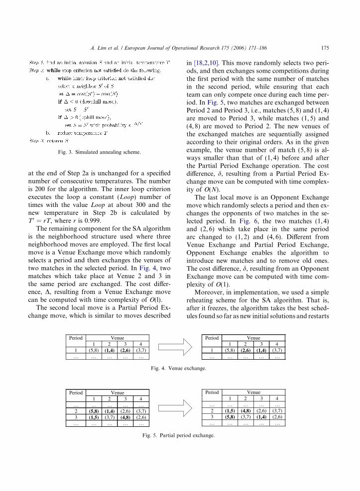
Fig. 3. Simulated annealing scheme.


at the end of Step 2a is unchanged for a specifiednumber of consecutive temperatures. The numberis 200 for the algorithm. The inner loop criterionexecutes the loop a constant (Loop) number oftimes with the value Loop at about 300 and thenew temperature in Step 2b is calculated byT 0 = rT, where r is 0.999.

The remaining component for the SA algorithmis the neighborhood structure used where threeneighborhood moves are employed. The first localmove is a Venue Exchange move which randomlyselects a period and then exchanges the venues oftwo matches in the selected period. In Fig. 4, twomatches which take place at Venue 2 and 3 inthe same period are exchanged. The cost differ-ence, D, resulting from a Venue Exchange movecan be computed with time complexity of O(l).

The second local move is a Partial Period Ex-change move, which is similar to moves described

VenuePeriod1 2 3 4

1 (5,8) (1,4) (2,6) (3,7)… … … … …

Fig. 4. Venue e

VenuePeriod1 2 3 4

… … … … … 2 (5,8) (1,4) (2,6) (3,7)3 (1,5) (3,7) (4,8) (2,6)

… … … … …

Fig. 5. Partial peri

in [18,2,10]. This move randomly selects two peri-ods, and then exchanges some competitions duringthe first period with the same number of matchesin the second period, while ensuring that eachteam can only compete once during each time per-iod. In Fig. 5, two matches are exchanged betweenPeriod 2 and Period 3, i.e., matches (5, 8) and (1, 4)are moved to Period 3, while matches (1, 5) and(4, 8) are moved to Period 2. The new venues ofthe exchanged matches are sequentially assignedaccording to their original orders. As in the givenexample, the venue number of match (5, 8) is al-ways smaller than that of (1, 4) before and afterthe Partial Period Exchange operation. The costdifference, d, resulting from a Partial Period Ex-change move can be computed with time complex-ity of O(N).

The last local move is an Opponent Exchangemove which randomly selects a period and then ex-changes the opponents of two matches in the se-lected period. In Fig. 6, the two matches (1, 4)and (2, 6) which take place in the same periodarc changed to (1, 2) and (4, 6). Different fromVenue Exchange and Partial Period Exchange,Opponent Exchange enables the algorithm tointroduce new matches and to remove old ones.The cost difference, d, resulting from an OpponentExchange move can be computed with time com-plexity of O(1).

Moreover, in implementation, we used a simplereheating scheme for the SA algorithm. That is,after it freezes, the algorithm takes the best sched-ules found so far as new initial solutions and restarts

VenuePeriod1 2 3 4

1 (5,8) (2,6) (1,4) (3,7)… … … … …

xchange.

VenuePeriod1 2 3 4

… … … … … 2 (1,5) (4,8) (2,6) (3,7)3 (5,8) (3,7) (1,4) (2,6)

… … … … …

od exchange.

VenuePeriod1 2 3 4

1 (5,8) (1,2) (4,6) (3,7)… … … … …

VenuePeriod1 2 3 4

1 (5,8) (1,4) (2,6) (3,7)… … … … …

Fig. 6. Opponent exchange.


the search process with initial parameter settings, aslong as the number of reheatings do not exceed aprescribed value, which was set as 200.

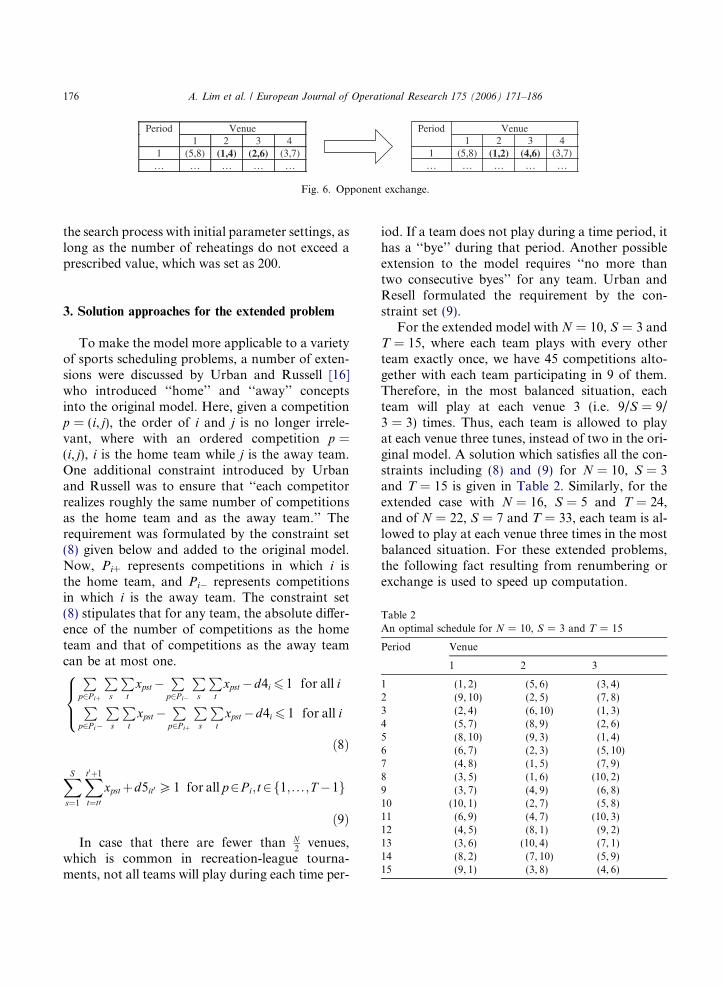
Table 2An optimal schedule for N = 10, S = 3 and T = 15

Period Venue

1 2 3

1 (1, 2) (5, 6) (3, 4)2 (9, 10) (2, 5) (7, 8)3 (2, 4) (6, 10) (1, 3)4 (5, 7) (8, 9) (2, 6)5 (8, 10) (9, 3) (1, 4)6 (6, 7) (2, 3) (5, 10)7 (4, 8) (1, 5) (7, 9)8 (3, 5) (1, 6) (10, 2)9 (3, 7) (4, 9) (6, 8)10 (10, 1) (2, 7) (5, 8)11 (6, 9) (4, 7) (10, 3)12 (4, 5) (8, 1) (9, 2)13 (3, 6) (10, 4) (7, 1)14 (8, 2) (7, 10) (5, 9)15 (9, 1) (3, 8) (4, 6)

3. Solution approaches for the extended problem

To make the model more applicable to a varietyof sports scheduling problems, a number of exten-sions were discussed by Urban and Russell [16]who introduced ‘‘home’’ and ‘‘away’’ conceptsinto the original model. Here, given a competitionp = (i, j), the order of i and j is no longer irrele-vant, where with an ordered competition p =(i, j), i is the home team while j is the away team.One additional constraint introduced by Urbanand Russell was to ensure that ‘‘each competitorrealizes roughly the same number of competitionsas the home team and as the away team.’’ Therequirement was formulated by the constraint set(8) given below and added to the original model.Now, Pi+ represents competitions in which i isthe home team, and Pi� represents competitionsin which i is the away team. The constraint set(8) stipulates that for any team, the absolute differ-ence of the number of competitions as the hometeam and that of competitions as the away teamcan be at most one.P

p2P iþ

Ps

Pt

xpst�P

p2P i�

Ps

Pt

xpst�d4i6 1 for all i

Pp2P i�

Ps

Pt

xpst�P

p2P iþ

Ps

Pt

xpst�d4i6 1 for all i

8><>:

ð8Þ

XS

s¼1

Xt0þ1

t¼t0xpstþd5it0 P1 for all p2P i;t2f1; . . . ;T �1g

ð9ÞIn case that there are fewer than N

2venues,

which is common in recreation-league tourna-ments, not all teams will play during each time per-

iod. If a team does not play during a time period, ithas a ‘‘bye’’ during that period. Another possibleextension to the model requires ‘‘no more thantwo consecutive byes’’ for any team. Urban andResell formulated the requirement by the con-straint set (9).

For the extended model with N = 10, S = 3 andT = 15, where each team plays with every otherteam exactly once, we have 45 competitions alto-gether with each team participating in 9 of them.Therefore, in the most balanced situation, eachteam will play at each venue 3 (i.e. 9/S = 9/3 = 3) times. Thus, each team is allowed to playat each venue three tunes, instead of two in the ori-ginal model. A solution which satisfies all the con-straints including (8) and (9) for N = 10, S = 3and T = 15 is given in Table 2. Similarly, for theextended case with N = 16, S = 5 and T = 24,and of N = 22, S = 7 and T = 33, each team is al-lowed to play at each venue three times in the mostbalanced situation. For these extended problems,the following fact resulting from renumbering orexchange is used to speed up computation.


Fact 5. There exists an optimal solution with the

following property: competitions at Venue 1 to S

during the first period are (1, 2), (3, 4), . . .(2S � 1, 2S), respectively.

Theorem 6. For any schedule C which satisfies all

constraints except those in the constraint set (8),

the algorithm SWITCH generates a schedule which

satisfies all constraints in (8) without violating any

constraints in the other constraint sets.

Given an ordered competition p = (i, j), algo-rithm SWITCH exchanges i and j if the circulardistance from j to i is less than or equal to(N � 1)/2. The circular distance from team j toteam i is (i � j) if it is non-negative, (i � j + N)otherwise. For example, if N = 10, the circular dis-tance from 8 to 2 is 4 (i.e. 2 � 8 + 10). AlgorithmSWITCH ensures that for any team x, when x

plays team y such that the circular distance fromx to y is not larger than (N � 1)/2, x is alwaysthe home team. There are altogether (N � 1)/2such y�s. SWITCH also ensures that for any teamx, when x plays with team y such that the circulardistance from y to x is not larger than (N � 1)/2, x

is always the away team.Again, there are altogether (N � 1)/2 such y�s.

Therefore, for any team x, the absolute differenceof the number of competitions as the home teamand that of competitions as the away team willbe at most one. For example, in the case N = 10,Team 8 is away when it plays with any team inthe set {4, 5, 6, 7}. Meanwhile, it is home whenplaying with any team in the set {9, 10, 1, 2}. Theorder of 3 and 8 is arbitrary, since the absolute dif-ference will be at most 1 no matter what the orderis. Therefore, SWITCH generates a schedule whichsatisfies all constraints in set (8) without violatingany additional constraint in other constraint setssince none of them is defined by the home/awayrules.

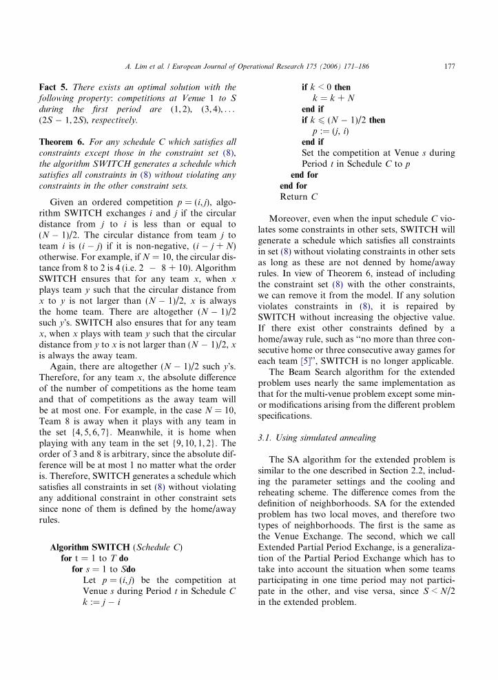
Algorithm SWITCH (Schedule C)
for t = 1 to T do
for s = 1 to Sdo
Let p = (i, j) be the competition atVenue s during Period t in Schedule C
k := j � i

if k < 0 then

k = k + N

end if

if k 6 (N � 1)/2 then

p := (j, i)end if

Set the competition at Venue s duringPeriod t in Schedule C to p

end for

end for

Return C

Moreover, even when the input schedule C vio-lates some constraints in other sets, SWITCH willgenerate a schedule which satisfies all constraintsin set (8) without violating constraints in other setsas long as these are not denned by home/awayrules. In view of Theorem 6, instead of includingthe constraint set (8) with the other constraints,we can remove it from the model. If any solutionviolates constraints in (8), it is repaired bySWITCH without increasing the objective value.If there exist other constraints defined by ahome/away rule, such as ‘‘no more than three con-secutive home or three consecutive away games foreach team [5]’’, SWITCH is no longer applicable.

The Beam Search algorithm for the extendedproblem uses nearly the same implementation asthat for the multi-venue problem except some min-or modifications arising from the different problemspecifications.

3.1. Using simulated annealing

The SA algorithm for the extended problem issimilar to the one described in Section 2.2, includ-ing the parameter settings and the cooling andreheating scheme. The difference comes from thedefinition of neighborhoods. SA for the extendedproblem has two local moves, and therefore twotypes of neighborhoods. The first is the same asthe Venue Exchange. The second, which we callExtended Partial Period Exchange, is a generaliza-tion of the Partial Period Exchange which has totake into account the situation when some teamsparticipating in one time period may not partici-pate in the other, and vise versa, since S < N/2in the extended problem.

VenuePeriod1 2 3

… … … …2 (1,2) (3,4) (5,6)3 (7,8) (9,10) (2,4)

… … … …

VenuePeriod1 2 3

… … … …2 (7,8) (2,4) (5,6)3 (1,2) (9,10) (3,4)

… … … …

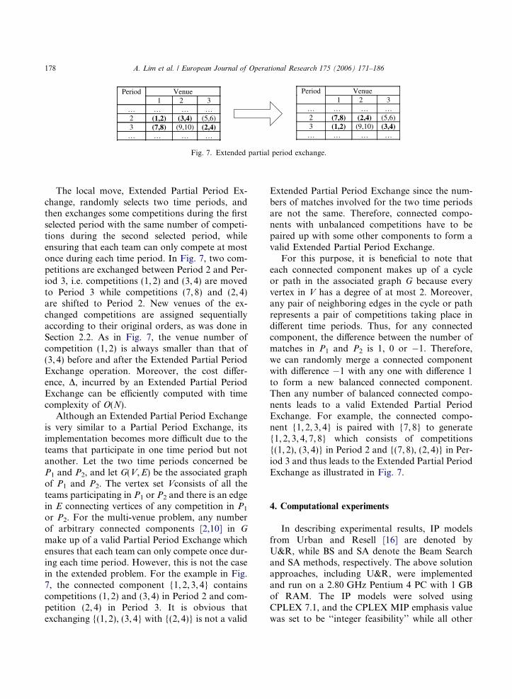
Fig. 7. Extended partial period exchange.


The local move, Extended Partial Period Ex-change, randomly selects two time periods, andthen exchanges some competitions during the firstselected period with the same number of competi-tions during the second selected period, whileensuring that each team can only compete at mostonce during each time period. In Fig. 7, two com-petitions are exchanged between Period 2 and Per-iod 3, i.e. competitions (1, 2) and (3, 4) are movedto Period 3 while competitions (7, 8) and (2, 4)are shifted to Period 2. New venues of the ex-changed competitions are assigned sequentiallyaccording to their original orders, as was done inSection 2.2. As in Fig. 7, the venue number ofcompetition (1, 2) is always smaller than that of(3, 4) before and after the Extended Partial PeriodExchange operation. Moreover, the cost differ-ence, D, incurred by an Extended Partial PeriodExchange can be efficiently computed with timecomplexity of O(N).

Although an Extended Partial Period Exchangeis very similar to a Partial Period Exchange, itsimplementation becomes more difficult due to theteams that participate in one time period but notanother. Let the two time periods concerned beP1 and P2, and let G(V, E) be the associated graphof P1 and P2. The vertex set Vconsists of all theteams participating in P1 or P2 and there is an edgein E connecting vertices of any competition in P1

or P2. For the multi-venue problem, any numberof arbitrary connected components [2,10] in G

make up of a valid Partial Period Exchange whichensures that each team can only compete once dur-ing each time period. However, this is not the casein the extended problem. For the example in Fig.7, the connected component {1, 2, 3, 4} containscompetitions (1, 2) and (3, 4) in Period 2 and com-petition (2, 4) in Period 3. It is obvious thatexchanging {(1, 2), (3, 4} with {(2, 4)} is not a valid

Extended Partial Period Exchange since the num-bers of matches involved for the two time periodsare not the same. Therefore, connected compo-nents with unbalanced competitions have to bepaired up with some other components to form avalid Extended Partial Period Exchange.

For this purpose, it is beneficial to note thateach connected component makes up of a cycleor path in the associated graph G because everyvertex in V has a degree of at most 2. Moreover,any pair of neighboring edges in the cycle or pathrepresents a pair of competitions taking place indifferent time periods. Thus, for any connectedcomponent, the difference between the number ofmatches in P1 and P2 is 1, 0 or �1. Therefore,we can randomly merge a connected componentwith difference �1 with any one with difference 1to form a new balanced connected component.Then any number of balanced connected compo-nents leads to a valid Extended Partial PeriodExchange. For example, the connected compo-nent {1, 2, 3, 4} is paired with {7, 8} to generate{1, 2, 3, 4, 7, 8} which consists of competitions{(1, 2), (3, 4)} in Period 2 and {(7, 8), (2, 4)} in Per-iod 3 and thus leads to the Extended Partial PeriodExchange as illustrated in Fig. 7.

4. Computational experiments

In describing experimental results, IP modelsfrom Urban and Resell [16] are denoted byU&R, while BS and SA denote the Beam Searchand SA methods, respectively. The above solutionapproaches, including U&R, were implementedand run on a 2.80 GHz Pentium 4 PC with 1 GBof RAM. The IP models were solved usingCPLEX 7.1, and the CPLEX MIP emphasis valuewas set to be ‘‘integer feasibility’’ while all other


parameters were set as their default values wherepreliminary results revealed that the IP modelsachieved better results when the MIP emphasiswas ‘‘integer feasibility’’. For example, the runningtime of U&R was 117.24 seconds when MIP was‘‘integer feasibility’’ and 1130.17 seconds whenMIP was ‘‘optimality’’ for the case N = 10. Lastly,the BS and SA algorithms were implemented inC++. The running time limit was 86 400 seconds(24 hours) for U&R. The SA algorithm was run10 times due to its randomized nature. Moreover,the running time of SA includes the BS runningtime since the initial solutions of SA were gener-ated by the beam search algorithm.

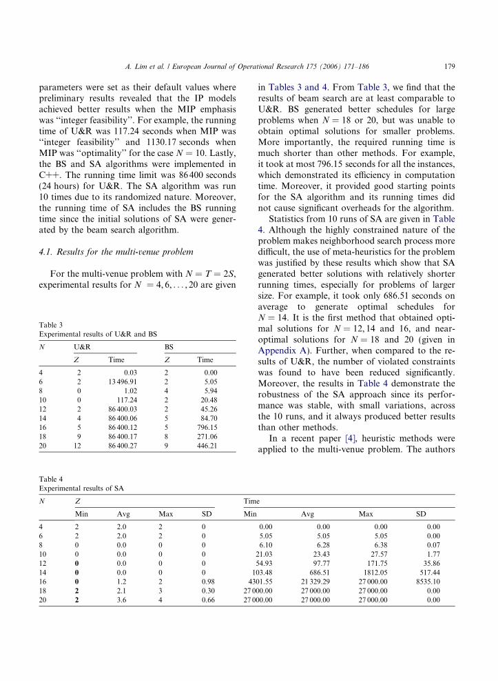
4.1. Results for the multi-venue problem

For the multi-venue problem with N = T = 2S,experimental results for N = 4, 6, . . . , 20 are given

Table 3Experimental results of U&R and BS

N U&R BS

Z Time Z Time

4 2 0.03 2 0.006 2 13 496.91 2 5.058 0 1.02 4 5.9410 0 117.24 2 20.4812 2 86 400.03 2 45.2614 4 86 400.06 5 84.7016 5 86 400.12 5 796.1518 9 86 400.17 8 271.0620 12 86 400.27 9 446.21

Table 4Experimental results of SA

N Z Tim

Min Avg Max SD Min

4 2 2.0 2 06 2 2.0 2 08 0 0.0 0 010 0 0.0 0 012 0 0.0 0 014 0 0.0 0 0 116 0 1.2 2 0.98 4318 2 2.1 3 0.30 27 020 2 3.6 4 0.66 27 0

in Tables 3 and 4. From Table 3, we find that theresults of beam search are at least comparable toU&R. BS generated better schedules for largeproblems when N = 18 or 20, but was unable toobtain optimal solutions for smaller problems.More importantly, the required running time ismuch shorter than other methods. For example,it took at most 796.15 seconds for all the instances,which demonstrated its efficiency in computationtime. Moreover, it provided good starting pointsfor the SA algorithm and its running times didnot cause significant overheads for the algorithm.

Statistics from 10 runs of SA are given in Table4. Although the highly constrained nature of theproblem makes neighborhood search process moredifficult, the use of meta-heuristics for the problemwas justified by these results which show that SAgenerated better solutions with relatively shorterrunning times, especially for problems of largersize. For example, it took only 686.51 seconds onaverage to generate optimal schedules forN = 14. It is the first method that obtained opti-mal solutions for N = 12, 14 and 16, and near-optimal solutions for N = 18 and 20 (given inAppendix A). Further, when compared to the re-sults of U&R, the number of violated constraintswas found to have been reduced significantly.Moreover, the results in Table 4 demonstrate therobustness of the SA approach since its perfor-mance was stable, with small variations, acrossthe 10 runs, and it always produced better resultsthan other methods.

In a recent paper [4], heuristic methods wereapplied to the multi-venue problem. The authors

e

Avg Max SD

0.00 0.00 0.00 0.005.05 5.05 5.05 0.006.10 6.28 6.38 0.07

21.03 23.43 27.57 1.7754.93 97.77 171.75 35.8603.48 686.51 1812.05 517.4401.55 21 329.29 27 000.00 8535.1000.00 27 000.00 27 000.00 0.0000.00 27 000.00 27 000.00 0.00


stated that ‘‘We have carried out experiments . . .for problems up to N = 20. The algorithm is capa-ble of producing perfectly balanced schedules forproblems of size N equal to 8, 10 and 12. It alsofinds the optimal solutions for the cases where Nequals 4 and 6. For the rest of the cases, so far,the algorithm is able to generate feasible scheduleswith low cost (between 8 and 18).’’ It is clear thatthe SA results here are superior than those in [4].With the SA algorithm, the penalty, Z, is 0 for in-stances with 8 to 16 teams and at most 2 for in-stances with up to 20 teams.

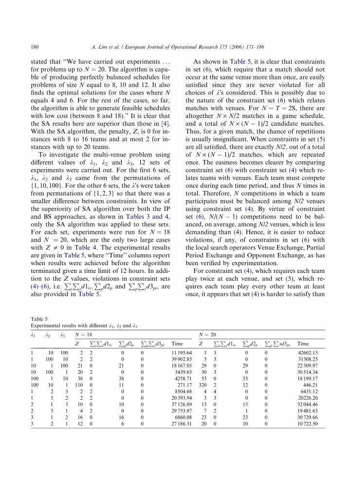
To investigate the multi-venue problem usingdifferent values of k1, k2 and k3, 12 sets ofexperiments were carried out. For the first 6 sets,k1, k2 and k3 came from the permutations of{1, 10, 100}. For the other 6 sets, the k�s were takenfrom permutations of {1, 2, 3} so that there was asmaller difference between constraints. In view ofthe superiority of SA algorithm over both the IPand BS approaches, as shown in Tables 3 and 4,only the SA algorithm was applied to these sets.For each set, experiments were run for N = 18and N = 20, which are the only two large caseswith Z 5 0 in Table 4. The experimental resultsare given in Table 5, where ‘‘Time’’ columns reportwhen results were achieved before the algorithmterminated given a time limit of 12 hours. In addi-tion to the Z values, violations in constraint sets(4)–(6), i.e.

Pi

Psd1is;

Ppd2p and

Pp

Psd3ps, are

also provided in Table 5.

Table 5Experimental results with different k1, k2 and k3

k1 k2 k3 N = 18

ZP

i

Psd1is

Ppd2p

Pp

Psd3ps Time

1 10 100 2 2 0 0 11 1951 100 10 2 2 0 0 39 90210 1 100 21 0 21 0 18 16710 100 1 20 2 0 0 5439100 1 10 38 0 38 0 4258100 10 1 110 0 11 0 2711 2 3 2 2 0 0 85041 3 2 2 2 0 0 20 3932 1 3 10 0 10 0 37 1262 3 1 4 2 0 0 29 7533 1 2 16 0 16 0 68603 2 1 12 0 6 0 27 186

As shown in Table 5, it is clear that constraintsin set (6), which require that a match should notoccur at the same venue more than once, are easilysatisfied since they are never violated for allchoices of k�s considered. This is possibly due tothe nature of the constraint set (6) which relatesmatches with venues. For N = T = 2S, there arealtogether N · N/2 matches in a game schedule,and a total of N · (N � 1)/2 candidate matches.Thus, for a given match, the chance of repetitionsis usually insignificant. When constraints in set (5)are all satisfied, there are exactly N/2, out of a totalof N · (N � 1)/2 matches, which are repeatedonce. The easiness becomes clearer by comparingconstraint set (6) with constraint set (4) which re-lates teams with venues. Each team must competeonce during each time period, and thus N times intotal. Therefore, N competitions in which a teamparticipates must be balanced among N/2 venuesusing constraint set (4). By virtue of constraintset (6), N/(N � 1) competitions need to be bal-anced, on average, among N/2 venues, which is lessdemanding than (4). Hence, it is easier to reduceviolations, if any, of constraints in set (6) withthe local search operators Venue Exchange, PartialPeriod Exchange and Opponent Exchange, as hasbeen verified by experimentation.

For constraint set (4), which requires each teamplay twice at each venue, and set (5), which re-quires each team play every other team at leastonce, it appears that set (4) is harder to satisfy than

N = 20

ZP

i

Psd1is

Ppd2p

Pp

Psd3ps Time

.64 3 3 0 0 42602.13

.85 3 3 0 0 31308.25

.05 29 0 29 0 22 309.97

.65 30 3 0 0 30 514.34

.71 53 0 53 0 18 199.17

.17 320 2 12 0 446.21

.68 4 4 0 0 6431.12

.94 3 3 0 0 20226.20

.89 13 0 13 0 32 044.46

.97 7 2 1 0 19 481.63

.08 23 0 23 0 30 729.66

.31 20 0 10 0 10 722.50

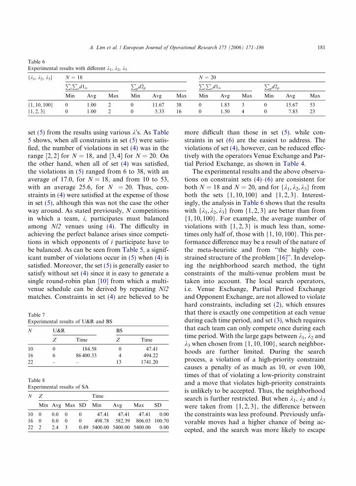
Table 6Experimental results with different k1, k2, k3

{k1, k2, k3} N = 18 N = 20P

i

Psd1is

Ppd2p

Pi

Psd1is

Ppd2p

Min Avg Max Min Avg Max Min Avg Max Min Avg Max

{1, 10, 100} 0 1.00 2 0 11.67 38 0 1.83 3 0 15.67 53{1, 2, 3} 0 1.00 2 0 5.33 16 0 1.50 4 0 7.83 23


set (5) from the results using various k�s. As Table5 shows, when all constraints in set (5) were satis-fied, the number of violations in set (4) was in therange [2, 2] for N = 18, and [3, 4] for N = 20. Onthe other hand, when all of set (4) was satisfied,the violations in (5) ranged from 6 to 38, with anaverage of 17.0, for N = 18, and from 10 to 53,with an average 25.6, for N = 20. Thus, con-straints in (4) were satisfied at the expense of thosein set (5), although this was not the case the otherway around. As stated previously, N competitionsin which a team, i, participates must balancedamong N/2 venues using (4). The difficulty inachieving the perfect balance arises since competi-tions in which opponents of i participate have tobe balanced. As can be seen from Table 5, a signif-icant number of violations occur in (5) when (4) issatisfied. Moreover, the set (5) is generally easier tosatisfy without set (4) since it is easy to generate asingle round-robin plan [10] from which a multi-venue schedule can be derived by repeating N/2

matches. Constraints in set (4) are believed to be

Table 7Experimental results of U&R and BS

N U&R BS

Z Time Z Time

10 0 184.58 0 47.4116 6 86 400.33 4 494.2222 – – 13 1741.20

Table 8Experimental results of SA

N Z Time

Min Avg Max SD Min Avg Max SD

10 0 0.0 0 0 47.41 47.41 47.41 0.0016 0 0.0 0 0 498.78 582.39 806.03 100.7022 2 2.4 3 0.49 5400.00 5400.00 5400.00 0.00

more difficult than those in set (5). while con-straints in set (6) are the easiest to address. Theviolations of set (4), however, can be reduced effec-tively with the operators Venue Exchange and Par-tial Period Exchange, as shown in Table 4.

The experimental results and the above observa-tions on constraint sets (4)–(6) are consistent forboth N = 18 and N = 20, and for {k1,k2,k3} fromboth the sets {1, 10, 100} and {1, 2, 3}. Interest-ingly, the analysis in Table 6 shows that the resultswith {k1,k2,k3} from {1, 2, 3} are better than from{1, 10, 100}. For example, the average number ofviolations with {1, 2, 3} is much less than, some-times only half of, those with {1, 10, 100}. This per-formance difference may be a result of the nature ofthe meta-heuristic and from ‘‘the highly con-strained structure of the problem [16]’’. In develop-ing the neighborhood search method, the tightconstraints of the multi-venue problem must betaken into account. The local search operators,i.e. Venue Exchange, Partial Period Exchangeand Opponent Exchange, are not allowed to violatehard constraints, including set (2), which ensuresthat there is exactly one competition at each venueduring each time period, and set (3), which requiresthat each team can only compete once during eachtime period. With the large gaps between k1, k2 andk3 when chosen from {1, 10, 100}, search neighbor-hoods are further limited. During the searchprocess, a violation of a high-priority constraintcauses a penalty of as much as 10, or even 100,times of that of violating a low-priority constraintand a move that violates high-priority constraintsis unlikely to be accepted. Thus, the neighborhoodsearch is further restricted. But when k1, k2 and k3

were taken from {1, 2, 3}, the difference betweenthe constraints was less profound. Previously unfa-vorable moves had a higher chance of being ac-cepted, and the search was more likely to escape


poor solution regions thus improving the final solu-tion quality as can be seen from the results in Ta-bles 5 and 6. Therefore, if the problem allows,narrower gaps between penalty coefficients are pre-ferred to larger ones when neighborhood searchmethods are applied to the highly-constrainedsports scheduling problem.

4.2. Results for the extended problem

For the extended problem where each team isallowed to play at each venue three times, exper-

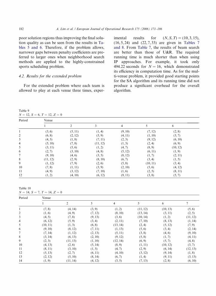
Table 9N = 12, S = 6, T = 12, Z = 0

Period Venue

1 2 3

1 (3, 6) (5, 11) (1, 4)2 (6, 8) (2, 12) (5, 9)3 (4, 5) (1, 8) (7, 11)4 (5, 10) (7, 8) (11, 12)5 (3, 11) (5, 6) (1, 2)6 (2, 7) (3, 10) (4, 8)7 (9, 10) (4, 6) (3, 5)8 (11, 12) (2, 9) (8, 10)9 (1, 12) (7, 9) (2, 6)10 (7, 8) (1, 11) (3, 9)11 (4, 9) (3, 12) (7, 10)12 (1, 2) (4, 10) (6, 12)

Table 10N = 14, S = 7, T = 14, Z = 0

Period Venue

1 2 3

1 (7, 8) (4, 14) (3, 9)2 (1, 6) (4, 9) (7, 12)3 (4, 5) (7, 8) (9, 13)4 (6, 12) (5, 9) (3, 4)5 (10, 11) (1, 3) (6, 8)6 (9, 10) (8, 12) (7, 11)7 (7, 14) (1, 12) (2, 13)8 (3, 14) (6, 13) (2, 10)9 (2, 3) (11, 13) (1, 10)10 (4, 13) (2, 6) (5, 14)11 (8, 11) (3, 10) (1, 5)12 (5, 13) (2, 7) (6, 11)13 (2, 12) (5, 10) (8, 14)14 (1, 9) (11, 14) (4, 12)

imental results for (N, S, T) = (10, 3, 15),(16, 5, 24) and (22, 7, 33) are given in Tables 7and 8. From Table 7, the results of beam searchare better than those of U&R. The requiredrunning time is much shorter than when usingIP approaches. For example, it took only494.22 seconds for N = 16, which demonstratedits efficiency in computation time. As for the mul-ti-venue problem, it provided good starting pointsfor the SA algorithm and its running time did notproduce a significant overhead for the overallalgorithm.

4 5 6

(9, 10) (7, 12) (2, 8)(4, 11) (1, 10) (3, 7)(2, 3) (9, 12) (6, 10)(1, 3) (2, 4) (6, 9)(4, 7) (8, 9) (10, 12)(5, 12) (6, 11) (1, 9)(8, 12) (1, 7) (2, 11)(6, 7) (3, 4) (1, 5)(5, 8) (10, 11) (3, 4)(2, 10) (5, 6) (4, 12)(1, 6) (2, 5) (8, 11)(9, 11) (3, 8) (5, 7)

4 5 6 7

(1, 2) (11, 12) (10, 13) (5, 6)(8, 10) (13, 14) (3, 11) (2, 5)(3, 6) (10, 14) (1, 2) (11, 12)(2, 11) (7, 10) (8, 13) (1, 14)

(13, 14) (2, 4) (5, 12) (7, 9)(1, 13) (5, 6) (3, 4) (2, 14)(5, 11) (3, 8) (4, 6) (9, 10)(9, 12) (5, 8) (1, 7) (4, 11)

(12, 14) (6, 9) (5, 7) (4, 8)(8, 9) (1, 11) (10, 12) (3, 7)(4, 7) (2, 9) (6, 14) (12, 13)(4, 10) (3, 12) (9, 14) (1, 8)(6, 7) (1, 4) (9, 11) (3, 13)(3, 5) (7, 13) (2, 8) (6, 10)

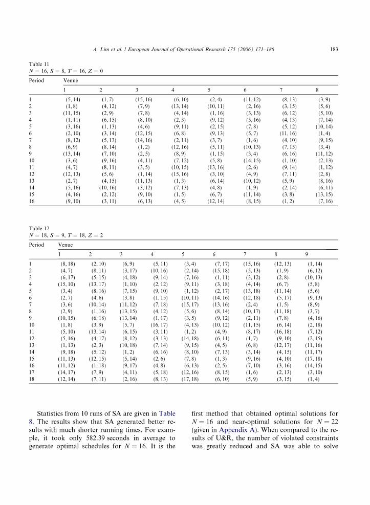
Table 11N = 16, S = 8, T = 16, Z = 0

Period Venue

1 2 3 4 5 6 7 8

1 (5, 14) (1, 7) (15, 16) (6, 10) (2, 4) (11, 12) (8, 13) (3, 9)2 (1, 8) (4, 12) (7, 9) (13, 14) (10, 11) (2, 16) (3, 15) (5, 6)3 (11, 15) (2, 9) (7, 8) (4, 14) (1, 16) (3, 13) (6, 12) (5, 10)4 (1, 11) (6, 15) (8, 10) (2, 3) (9, 12) (5, 16) (4, 13) (7, 14)5 (3, 16) (1, 13) (4, 6) (9, 11) (2, 15) (7, 8) (5, 12) (10, 14)6 (2, 10) (3, 14) (12, 15) (6, 8) (9, 13) (5, 7) (11, 16) (1, 4)7 (8, 12) (5, 13) (14, 16) (2, 11) (3, 7) (1, 6) (4, 10) (9, 15)8 (6, 9) (8, 14) (1, 2) (12, 16) (5, 11) (10, 13) (7, 15) (3, 4)9 (13, 14) (7, 10) (2, 5) (8, 9) (1, 15) (3, 4) (6, 16) (11, 12)10 (3, 6) (9, 16) (4, 11) (7, 12) (5, 8) (14, 15) (1, 10) (2, 13)11 (4, 7) (8, 11) (3, 5) (10, 15) (13, 16) (2, 6) (9, 14) (1, 12)12 (12, 13) (5, 6) (1, 14) (15, 16) (3, 10) (4, 9) (7, 11) (2, 8)13 (2, 7) (4, 15) (11, 13) (1, 3) (6, 14) (10, 12) (5, 9) (8, 16)14 (5, 16) (10, 16) (3, 12) (7, 13) (4, 8) (1, 9) (2, 14) (6, 11)15 (4, 16) (2, 12) (9, 10) (1, 5) (6, 7) (11, 14) (3, 8) (13, 15)16 (9, 10) (3, 11) (6, 13) (4, 5) (12, 14) (8, 15) (1, 2) (7, 16)

Table 12N = 18, S = 9, T = 18, Z = 2

Period Venue

1 2 3 4 5 6 7 8 9

1 (8, 18) (2, 10) (6, 9) (5, 11) (3, 4) (7, 17) (15, 16) (12, 13) (1, 14)2 (4, 7) (8, 11) (3, 17) (10, 16) (2, 14) (15, 18) (5, 13) (1, 9) (6, 12)3 (6, 17) (5, 15) (4, 18) (9, 14) (7, 16) (1, 11) (3, 12) (2, 8) (10, 13)4 (15, 10) (13, 17) (1, 10) (2, 12) (9, 11) (3, 18) (4, 14) (6, 7) (5, 8)5 (3, 4) (8, 16) (7, 15) (9, 10) (1, 12) (2, 17) (13, 18) (11, 14) (5, 6)6 (2, 7) (4, 6) (3, 8) (1, 15) (10, 11) (14, 16) (12, 18) (5, 17) (9, 13)7 (3, 6) (10, 14) (11, 12) (7, 18) (15, 17) (13, 16) (2, 4) (1, 5) (8, 9)8 (2, 9) (1, 16) (13, 15) (4, 12) (5, 6) (8, 14) (10, 17) (11, 18) (3, 7)9 (10, 15) (6, 18) (13, 14) (1, 17) (3, 5) (9, 12) (2, 11) (7, 8) (4, 16)10 (1, 8) (3, 9) (5, 7) (16, 17) (4, 13) (10, 12) (11, 15) (6, 14) (2, 18)11 (5, 10) (13, 14) (6, 15) (3, 11) (1, 2) (4, 9) (8, 17) (16, 18) (7, 12)12 (5, 16) (4, 17) (8, 12) (3, 13) (14, 18) (6, 11) (1, 7) (9, 10) (2, 15)13 (1, 13) (2, 3) (10, 18) (7, 14) (9, 15) (4, 5) (6, 8) (12, 17) (11, 16)14 (9, 18) (5, 12) (1, 2) (6, 16) (8, 10) (7, 13) (3, 14) (4, 15) (11, 17)15 (11, 13) (12, 15) (5, 14) (2, 6) (7, 8) (1, 3) (9, 16) (4, 10) (17, 18)16 (11, 12) (1, 18) (9, 17) (4, 8) (6, 13) (2, 5) (7, 10) (3, 16) (14, 15)17 (14, 17) (7, 9) (4, 11) (5, 18) (12, 16) (8, 15) (1, 6) (2, 13) (3, 10)18 (12, 14) (7, 11) (2, 16) (8, 13) (17, 18) (6, 10) (5, 9) (3, 15) (1, 4)


Statistics from 10 runs of SA are given in Table8. The results show that SA generated better re-sults with much shorter running times. For exam-ple, it took only 582.39 seconds in average togenerate optimal schedules for N = 16. It is the

first method that obtained optimal solutions forN = 16 and near-optimal solutions for N = 22(given in Appendix A). When compared to the re-sults of U&R, the number of violated constraintswas greatly reduced and SA was able to solve

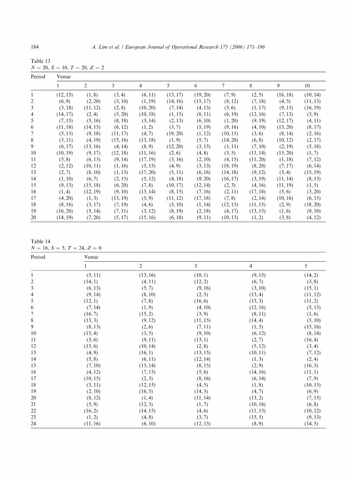
Table 13N = 20, S = 10, T = 20, Z = 2

Period Venue

1 2 3 4 5 6 7 8 9 10

1 (12, 15) (1, 8) (3, 4) (6, 11) (13, 17) (19, 20) (7, 9) (2, 5) (16, 18) (10, 14)2 (6, 9) (2, 20) (3, 10) (1, 19) (14, 16) (15, 17) (8, 12) (7, 18) (4, 5) (11, 13)3 (3, 18) (11, 12) (2, 8) (10, 20) (7, 14) (4, 13) (5, 6) (1, 17) (9, 15) (16, 19)4 (14, 17) (2, 4) (5, 20) (10, 18) (1, 15) (8, 11) (6, 19) (12, 16) (7, 13) (3, 9)5 (7, 15) (5, 16) (8, 18) (3, 14) (2, 13) (6, 10) (1, 20) (9, 19) (12, 17) (4, 11)6 (11, 18) (14, 15) (6, 12) (1, 2) (3, 7) (5, 19) (9, 16) (4, 10) (13, 20) (8, 17)7 (5, 13) (9, 18) (11, 17) (4, 7) (19, 20) (1, 12) (10, 15) (3, 6) (8, 14) (2, 16)8 (3, 11) (4, 19) (15, 16) (13, 18) (1, 9) (5, 7) (14, 20) (6, 8) (10, 12) (2, 17)9 (6, 17) (13, 16) (4, 14) (8, 9) (12, 20) (3, 15) (1, 11) (7, 10) (2, 19) (5, 18)10 (10, 19) (9, 17) (12, 18) (11, 16) (2, 6) (4, 8) (3, 5) (13, 14) (15, 20) (1, 7)11 (5, 8) (6, 13) (9, 14) (17, 19) (3, 16) (2, 10) (4, 15) (11, 20) (1, 18) (7, 12)12 (2, 12) (10, 11) (1, 16) (5, 15) (4, 9) (3, 13) (18, 19) (8, 20) (7, 17) (6, 14)13 (2, 7) (8, 10) (1, 13) (17, 20) (5, 11) (6, 16) (14, 18) (9, 12) (3, 4) (15, 19)14 (1, 10) (6, 7) (2, 15) (5, 12) (4, 18) (9, 20) (16, 17) (3, 19) (11, 14) (8, 13)15 (9, 13) (15, 18) (6, 20) (7, 8) (10, 17) (12, 14) (2, 3) (4, 16) (11, 19) (1, 5)16 (1, 4) (12, 19) (9, 10) (13, 14) (8, 15) (7, 16) (2, 11) (17, 18) (5, 6) (3, 20)17 (4, 20) (1, 3) (13, 19) (5, 9) (11, 12) (17, 18) (7, 8) (2, 14) (10, 16) (6, 15)18 (8, 16) (3, 17) (7, 19) (4, 6) (5, 10) (1, 14) (12, 13) (11, 15) (2, 9) (18, 20)19 (16, 20) (5, 14) (7, 11) (3, 12) (8, 19) (2, 18) (4, 17) (13, 15) (1, 6) (9, 10)20 (14, 19) (7, 20) (5, 17) (15, 16) (6, 18) (9, 11) (10, 13) (1, 2) (3, 8) (4, 12)

Table 14N = 16, S = 5, T = 24, Z = 0

Period Venue

1 2 3 4 5

1 (5, 11) (13, 16) (10, 1) (9, 15) (14, 2)2 (14, 1) (4, 11) (12, 2) (6, 7) (3, 8)3 (6, 13) (5, 7) (9, 16) (3, 10) (15, 1)4 (9, 14) (8, 10) (2, 5) (13, 4) (11, 12)5 (12, 1) (7, 8) (16, 6) (15, 3) (11, 2)6 (7, 14) (1, 9) (4, 10) (12, 16) (5, 13)7 (16, 7) (15, 2) (3, 9) (8, 11) (1, 6)8 (13, 3) (9, 12) (11, 15) (14, 4) (5, 10)9 (8, 13) (2, 6) (7, 11) (1, 5) (15, 16)10 (15, 4) (3, 5) (9, 10) (6, 12) (8, 14)11 (3, 6) (9, 11) (13, 1) (2, 7) (16, 4)12 (15, 6) (10, 14) (2, 8) (5, 12) (3, 4)13 (4, 9) (16, 1) (13, 15) (10, 11) (7, 12)14 (5, 8) (6, 11) (12, 14) (1, 3) (2, 4)15 (7, 10) (13, 14) (8, 15) (2, 9) (16, 3)16 (4, 12) (7, 13) (5, 6) (14, 16) (11, 1)17 (10, 15) (2, 3) (8, 16) (6, 14) (7, 9)18 (3, 11) (12, 15) (4, 5) (1, 8) (10, 13)19 (2, 10) (16, 5) (14, 3) (4, 7) (6, 9)20 (8, 12) (1, 4) (11, 14) (13, 2) (7, 15)21 (5, 9) (12, 3) (1, 7) (10, 16) (6, 8)22 (16, 2) (14, 15) (4, 6) (11, 13) (10, 12)23 (1, 2) (4, 8) (3, 7) (15, 5) (9, 13)24 (11, 16) (6, 10) (12, 13) (8, 9) (14, 5)


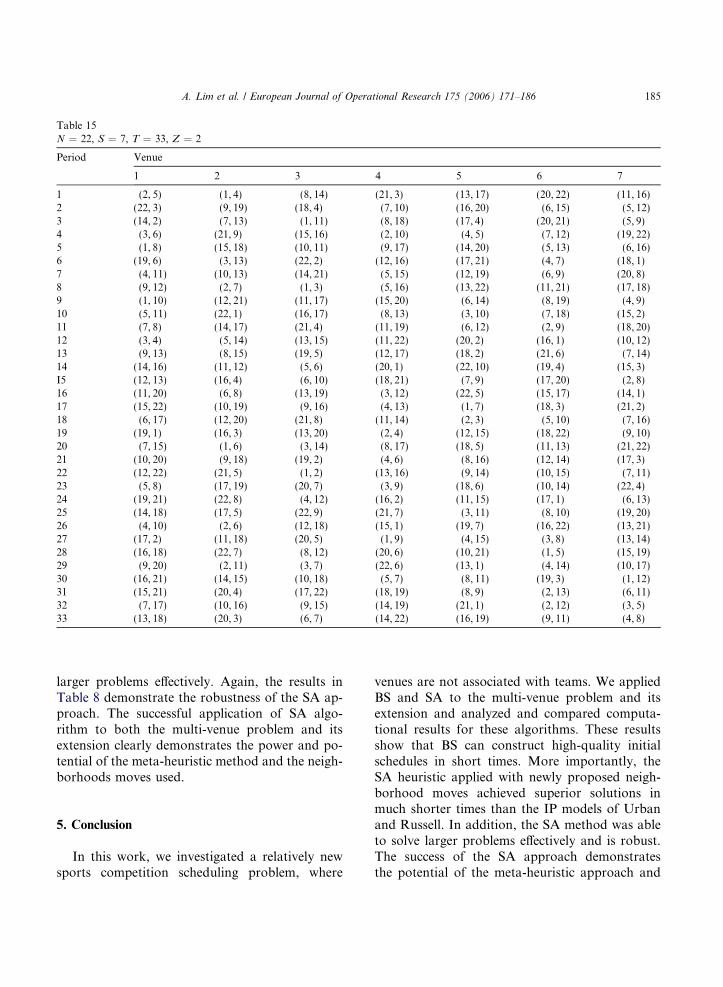
Table 15N = 22, S = 7, T = 33, Z = 2

Period Venue

1 2 3 4 5 6 7

1 (2, 5) (1, 4) (8, 14) (21, 3) (13, 17) (20, 22) (11, 16)2 (22, 3) (9, 19) (18, 4) (7, 10) (16, 20) (6, 15) (5, 12)3 (14, 2) (7, 13) (1, 11) (8, 18) (17, 4) (20, 21) (5, 9)4 (3, 6) (21, 9) (15, 16) (2, 10) (4, 5) (7, 12) (19, 22)5 (1, 8) (15, 18) (10, 11) (9, 17) (14, 20) (5, 13) (6, 16)6 (19, 6) (3, 13) (22, 2) (12, 16) (17, 21) (4, 7) (18, 1)7 (4, 11) (10, 13) (14, 21) (5, 15) (12, 19) (6, 9) (20, 8)8 (9, 12) (2, 7) (1, 3) (5, 16) (13, 22) (11, 21) (17, 18)9 (1, 10) (12, 21) (11, 17) (15, 20) (6, 14) (8, 19) (4, 9)10 (5, 11) (22, 1) (16, 17) (8, 13) (3, 10) (7, 18) (15, 2)11 (7, 8) (14, 17) (21, 4) (11, 19) (6, 12) (2, 9) (18, 20)12 (3, 4) (5, 14) (13, 15) (11, 22) (20, 2) (16, 1) (10, 12)13 (9, 13) (8, 15) (19, 5) (12, 17) (18, 2) (21, 6) (7, 14)14 (14, 16) (11, 12) (5, 6) (20, 1) (22, 10) (19, 4) (15, 3)I5 (12, 13) (16, 4) (6, 10) (18, 21) (7, 9) (17, 20) (2, 8)16 (11, 20) (6, 8) (13, 19) (3, 12) (22, 5) (15, 17) (14, 1)17 (15, 22) (10, 19) (9, 16) (4, 13) (1, 7) (18, 3) (21, 2)18 (6, 17) (12, 20) (21, 8) (11, 14) (2, 3) (5, 10) (7, 16)19 (19, 1) (16, 3) (13, 20) (2, 4) (12, 15) (18, 22) (9, 10)20 (7, 15) (1, 6) (3, 14) (8, 17) (18, 5) (11, 13) (21, 22)21 (10, 20) (9, 18) (19, 2) (4, 6) (8, 16) (12, 14) (17, 3)22 (12, 22) (21, 5) (1, 2) (13, 16) (9, 14) (10, 15) (7, 11)23 (5, 8) (17, 19) (20, 7) (3, 9) (18, 6) (10, 14) (22, 4)24 (19, 21) (22, 8) (4, 12) (16, 2) (11, 15) (17, 1) (6, 13)25 (14, 18) (17, 5) (22, 9) (21, 7) (3, 11) (8, 10) (19, 20)26 (4, 10) (2, 6) (12, 18) (15, 1) (19, 7) (16, 22) (13, 21)27 (17, 2) (11, 18) (20, 5) (1, 9) (4, 15) (3, 8) (13, 14)28 (16, 18) (22, 7) (8, 12) (20, 6) (10, 21) (1, 5) (15, 19)29 (9, 20) (2, 11) (3, 7) (22, 6) (13, 1) (4, 14) (10, 17)30 (16, 21) (14, 15) (10, 18) (5, 7) (8, 11) (19, 3) (1, 12)31 (15, 21) (20, 4) (17, 22) (18, 19) (8, 9) (2, 13) (6, 11)32 (7, 17) (10, 16) (9, 15) (14, 19) (21, 1) (2, 12) (3, 5)33 (13, 18) (20, 3) (6, 7) (14, 22) (16, 19) (9, 11) (4, 8)


larger problems effectively. Again, the results inTable 8 demonstrate the robustness of the SA ap-proach. The successful application of SA algo-rithm to both the multi-venue problem and itsextension clearly demonstrates the power and po-tential of the meta-heuristic method and the neigh-borhoods moves used.

5. Conclusion

In this work, we investigated a relatively newsports competition scheduling problem, where

venues are not associated with teams. We appliedBS and SA to the multi-venue problem and itsextension and analyzed and compared computa-tional results for these algorithms. These resultsshow that BS can construct high-quality initialschedules in short times. More importantly, theSA heuristic applied with newly proposed neigh-borhood moves achieved superior solutions inmuch shorter times than the IP models of Urbanand Russell. In addition, the SA method was ableto solve larger problems effectively and is robust.The success of the SA approach demonstratesthe potential of the meta-heuristic approach and


the usefulness of the neighborhood moves for thehighly-constrained sports scheduling problem.

Appendix A

See Tables 9–15.

References

[1] E. Aarts, J. Korst, Simulated Annealing and BoltzmannMachines: A Stochastic Approach to Combinatorial Opti-mization and Neural Computing, Wiley, Chichester, 1989.

[2] A. Anagnostopoulos, L. Michel, P. Van Hentenryck, Y.Vergados. A simulated annealing approach to the travelingtournament problem, in: Proceedings of CPAIOR�03,2003.

[3] B.C. Ball, D.B. Webster, Optimal scheduling for even-numbered team Athletic Conference, AITE Transactions 9(1977) 161–169.

[4] E.K. Burke, D. de Werra, J.D. Landa Silva, C. Raess,Applying heuristic methods to schedule sports competi-tions on multiple venues, in: Proceedings PATAT�04,Pittsburgh, USA, 2004.

[5] K. Easton, G. Nemhauser, M. Trick, The travelingtournament problem description and benchmarks, in:Proceedings of the 7th International Conference on Prin-ciples and Practice of Constraint Programming, CP 2001,Paphos, Cyprus, 2001, pp. 580–584.

[6] M. Henz, Scheduling a major College Basketball Confer-ence: Revisited, Operations Research 49 (2000) 163–168.

[7] D.S. Johnson, C.R. Aragon, L.A. McGeoch, C. Schevon,Optimization by simulated annealing: An experimental

evaluation; Part I, graph partitioning, Operations Research37 (1989) 865–892.

[8] S. Kirkpatrick Jr., C.D. Gelatt, M.P. Vecchi, Optimizationby simulated annealing, Science 220 (1983) 671–680.

[9] P.J.M. Laarhoven, E.H.L. Aarts, Simulated Annealing:Theory and Applications, Reidel, Dordrecht, 1987.

[10] A. Lim, B. Rodrigues, X. Zhang, A simulated annealingand hill-climbing algorithm for the traveling tournamentproblem, Working Paper, Departmet of IEEM, HongKong University of Science and Technology, Hong Kong,2004.

[11] B.T. Lowerre, The HARPY Speech Recognition Sys-tem, PhD thesis, Carnegie-Mellon University, USA, April1976.

[12] G. Nemhauser, M. Trick, Scheduling a major CollegeBasketball Conference, Operations Research 46 (1998)1–8.

[13] K.J. Nurmela, P.R.J. Ostergard, Constructing coveringdesigns by simulated annealing. Technical report, DigitalSystems Laboratory, Helsinki University of Technology,Otaniemi, Finland, 1993.

[14] S. Rubin, The ARGOS Image Understanding System. PhDthesis, Carnegie-Mellon University, USA, April 1978.

[15] R.A. Russell, J.M. Lcung, Devising a cost effectiveschedule for a baseball league, Operations Research 42(1994) 614–625.

[16] T.L. Urban, R.A. Russell, Scheduling sports competitionson multiple venues, European Journal of OperationalResearch 148 (2003) 302–311.

[17] D. De Werra, L. Jacot-Descombes, P. Masson, A con-strained sports scheduling problem, Discrete AppliedMathematics 26 (1990) 41–49.

[18] X. Zhang, Constraint programming, simulated annealingand hill-climbing algorithm for traveling tournamentproblems, Technical report, School of Computing,National University of Singapore, 2002.

Documents

Scheduling sports competitions at multiple venues—Revisited