SCIENTIFIC VISUALIZATION

Lecture 3 part 1

Scientific Visualization GroupVisual Information Technology and ApplicationsLinköping University

CONTENTS

• Color mapping

• Contouring

– Marching Cubes in detail

– Effective searching

– Other algorithms

• Scalar generationInsight!

VISUALIZATION

RenderingArchive

Experiment

Computation

Computer-representation

Transformation

Image control

Process steering

Computational steering

TRANSFORMATIONS

• Structure

– Effects that the transformation has on the topology and geometry of the dataset

• Type

– The kind of data set the transformation is operating on

STRUCTURAL CLASSIFICATION

• Geometric transformations

– Alter input geometry but not topology

• Topological transformations

– Alter topology but not geometry and attribute

• Attribute transformations

– Converts attribute data or creates new attributes

• Combined transformations

– Changes both dataset structure and attributes

TYPE CLASSIFICATION

•Scalar algorithms

•Vector algorithms

•Tensor algorithms

•Modelling algorithms

COLOR MAPPPING

• Maps the scalar to a color (1D technique)

• Implemented using lookup tables indexed with the scalar value

• Lookup table specifies RGB or HSVA components

TRANSFER FUNCTIONS

• Instead of using a lookup table we could specify a “transfer function” mapping scalar values to RGB components

Red

value

I

Green

value

I

Blue

value

I

A VTK LOOKUP TABLE

• Insert values in table to enhance features

• Make sure you know the difference between colormaps and actorproperties

VtkLookupTable *lut=vtkLookupTable::New(); lut->SetHueRange(0.6667, 0.0); lut->SetSaturationRange(1.0, 1.0); lut->SetValueRange(1.0, 1.0) lut->SetNumberOfColors(256) lut->Build();

vtkPolyDataMapper *mapper=vtkPolyDataMapper::New();

mapper->SetLookupTable(lut); mapper->SetScalarRange(min,max)

COLOR MAPPING

See VTK book page 153!

CONTOURING

• A quadric function

• Constant function value defines surfaces in 3D

• Shows 3 isosurfaces

• Isosurface value used to map colors

CONTOURING

• Gives contours in 2D

• Gives iso-surfaces in 3D

• Several different methods exists

– We will deal with two for iso-surfaces

•Marching Cubes (Lorensen & Cline 1987)

•Surface reconstruction from planar contours (Fuchs et al 1977)

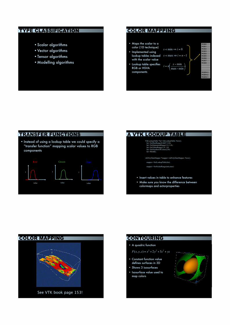
MARCHING CUBES

• Consider a cube (voxel) in the dataset

• We have three cases:

– All vertices above the iso-value

– All vertices below the iso-value

– Mixed above and below

• Binary label each node (above/below)

• Examine all possible cases of above or below for each vertex

• 8 vertices implies 256 possible cases

+

+

+

+

+ +

+

-

STEP 1:

• Consider a cube defined by eight data values

– four from slice K, and four from slice K+1

(i,j,k)

(i,j+1,k+1)

(i+1,j,k)

(i,j,k+1)

(i,j+1,k)(i+1,j+1,k)

(i+1,j+1,k+1)

(i+1,j,k+1)

Create Cube STEP 2:

• Binary classification of each vertex of the cube as to whether it lies

– Outside the surface (vertex value < iso-surface value)

– Inside the surface (vertex value >= iso-surface value)

8

10

8

5

108

10

5

T=9

T=7

Outside

Inside

Classify each voxel

STEP 3:

• Use the binary labeling of each vertex an 8-bit index. (256 cases)

8

10

8

5

108

10

5

T=9

T=7

11010000

11110011

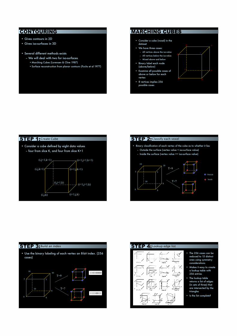
Build an index STEP 4: Lookup edge list

• The 256 cases can be reduced to 15 distinct ones using symmetry considerations

• Makes it easy to create a lookup table with 256 entries

• The lookup table returns a list of edges (in sets of three) that are intersected by the triangles

• Is the list complete?

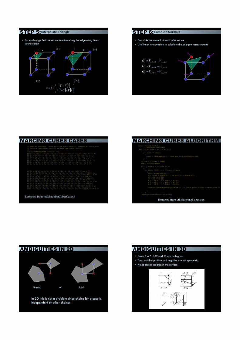
STEP 5:

• For each edge find the vertex location along the edge using linear interpolation

Interpolate Triangle Vertices

T=5 T=8

i i+1xi x i+1

STEP 6:

• Calculate the normal at each cube vertex

• Use linear interpolation to calculate the polygon vertex normal

Compute Normals

MARCING CUBES CASES// Edges to intersect. Three at a time form a triangle. Comments at end of line// indicate case number (0->255) and base case number (0->15).//static TRIANGLE_CASES triCases[] = { {{-1, -1, -1, -1, -1, -1, -1, -1, -1, -1, -1, -1, -1, -1, -1, -1}}, /* 0 0 */{{ 0, 3, 8, -1, -1, -1, -1, -1, -1, -1, -1, -1, -1, -1, -1, -1}}, /* 1 1 */{{ 0, 9, 1, -1, -1, -1, -1, -1, -1, -1, -1, -1, -1, -1, -1, -1}}, /* 2 1 */{{ 1, 3, 8, 9, 1, 8, -1, -1, -1, -1, -1, -1, -1, -1, -1, -1}}, /* 3 2 */{{ 1, 11, 2, -1, -1, -1, -1, -1, -1, -1, -1, -1, -1, -1, -1, -1}}, /* 4 1 */{{ 0, 3, 8, 1, 11, 2, -1, -1, -1, -1, -1, -1, -1, -1, -1, -1}}, /* 5 3 */{{ 9, 11, 2, 0, 9, 2, -1, -1, -1, -1, -1, -1, -1, -1, -1, -1}}, /* 6 2 */

.

.

.

{{ 3, 9, 0, 3, 10, 9, 1, 9, 2, 2, 9, 10, -1, -1, -1, -1}}, /* 245 3 */{{ 0, 10, 2, 8, 10, 0, -1, -1, -1, -1, -1, -1, -1, -1, -1, -1}}, /* 246 2 */{{ 3, 10, 2, -1, -1, -1, -1, -1, -1, -1, -1, -1, -1, -1, -1, -1}}, /* 247 1 */{{ 2, 8, 3, 2, 11, 8, 11, 9, 8, -1, -1, -1, -1, -1, -1, -1}}, /* 248 5 */{{ 9, 2, 11, 0, 2, 9, -1, -1, -1, -1, -1, -1, -1, -1, -1, -1}}, /* 249 2 */{{ 2, 8, 3, 2, 11, 8, 0, 8, 1, 1, 8, 11, -1, -1, -1, -1}}, /* 250 3 */{{ 1, 2, 11, -1, -1, -1, -1, -1, -1, -1, -1, -1, -1, -1, -1, -1}}, /* 251 1 */{{ 1, 8, 3, 9, 8, 1, -1, -1, -1, -1, -1, -1, -1, -1, -1, -1}}, /* 252 2 */{{ 0, 1, 9, -1, -1, -1, -1, -1, -1, -1, -1, -1, -1, -1, -1, -1}}, /* 253 1 */{{ 0, 8, 3, -1, -1, -1, -1, -1, -1, -1, -1, -1, -1, -1, -1, -1}}, /* 254 1 */{{-1, -1, -1, -1, -1, -1, -1, -1, -1, -1, -1, -1, -1, -1, -1, -1}}}; /* 255 0 */

Extracted from vtkMarchingCubesCases.h

MARCHING CUBES ALGORITHM value = values[contNum]; // Build the case table for ( ii=0, index = 0; ii < 8; ii++) { if ( s[ii] >= value ) { index |= CASE_MASK[ii]; // CASE_MASK {1,2,4,8,16,32,64,128} } } triCase = triCases + index; edge = triCase->edges;

for ( ; edge[0] > -1; edge += 3 ) { for (ii=0; ii<3; ii++) //insert triangle { vert = edges[edge[ii]]; t = (value - s[vert[0]]) / (s[vert[1]] - s[vert[0]]); x1 = pts[vert[0]]; x2 = pts[vert[1]]; x[0] = x1[0] + t * (x2[0] - x1[0]); x[1] = x1[1] + t * (x2[1] - x1[1]); x[2] = x1[2] + t * (x2[2] - x1[2]);

locator->InsertUniquePoint(x,PtIds[ii]) // Insert point in list & return point ID

} } newPolys->InsertNextCell(3,ptIds);

Extracted from vtkMarchingCubes.cxx

AMBIGUITIES IN 2D

Break! or Join!

In 2D this is not a problem since choice for a case is independent of other choices!

AMBIGUITIES IN 3D

• Cases 3,6,7,10,12 and 13 are ambigous

• Turns out that positive and negative are not symmetric

• Holes can be created in the surface!

SOLUTIONS

• Use marching tetrehedra

– Requires more trigangles

– Can create artificial bumps in iso-surfaces

• Use asymptotic decider

– looks at the variation of the scalar across the surface

• Use other complimentary cases (see paper by Montani et. al.)

MODIFIED COMPLIMENTARY

Can you find them in the lookup table?

MARCHING CUBES Summary

•Create a cube

•Classify each voxel

•Build an index

•Lookup edge list

• Interpolate triangle vertices

•Calculate and interpolate normals

NICE EXAMPLE

Now we deserve a nice example of Marching Cubes at work.

fMRI under meditation

Mantra-övningSpråktest

Mixed Reality for Surgery

fMRI demonstrator

• Use state of the art Canonical Correlation Analysis developed by CMIV (Friman et. al.)

• Improve methods to achieve real-time responses

• New approaches to data processing are needed.

• Realtime visualization and interaction

• Study bio feedback through visualization of a square which follows the point of focus of the eyes.

Experimental setup

SCIENTIFIC VISUALIZATION

Lecture 3 part 2

Scientific Visualization GroupVisual Information Technology and ApplicationsLinköping University

EFFICIENT SEARCHING

• With < 10% of the voxels contributing to the surface, it is a waste to look at every voxel

• A voxel can be specified in terms of its interval, its minimum and maximum values

• Define the span space!

SPAN SPACE

Plot each voxel according to maximum and minimum value

MA

XIM

UM

MINIMUMIso-value

Low gradient

High gradient

SPAN SPACE REPRESENTATION

•Kd-Trees

MA

XIM

UM

MINIMUM Split max axis

Split min axis

CONTOUR STITCHING

• Given: 2 two-dimensional closed curves

– Curve #1 has m points

– Curve #2 has n points

• Which point(s) does vertex j on curve one correspond to on curve two

j

?

?

A SOLUTION: • Fuchs, et al.

– Optimization problem

– Nice paper (graph

theory)

– 1 stitch consists of:

• 2 spans between

curves

• 1 contour segment

• Triangles

• Consistent normal directions

or

Fuchs et. al. Fuchs et. al.

• Left span

– P(i)Q(j) =>go up

• Right span (either)

– P(i+1) Q(j) => go down

– P(i)Q(j+1)=> go down

• Constraints

– Each contour segement is used once and only once

– If a span appears as a left span, then it must also appear as a right span

– If a span appears as a right span, then it must also appear as a left span

This produces an optimal surface from a topological point of view, i.e. no holes.

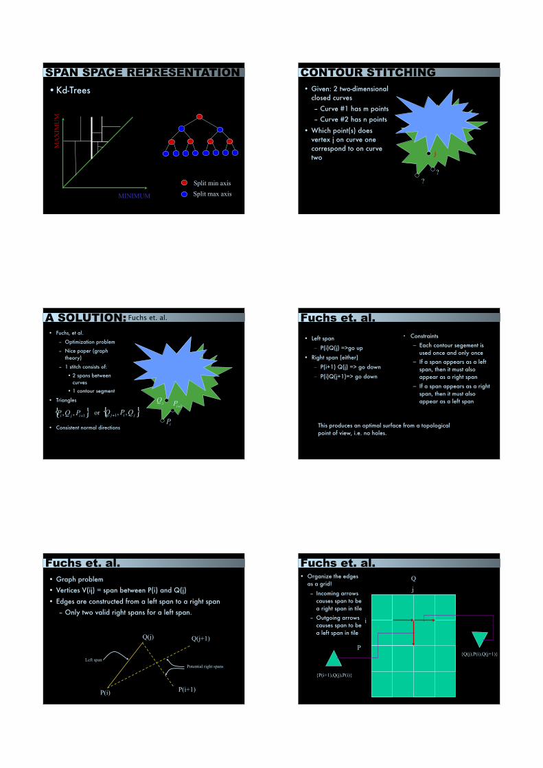
Fuchs et. al.

• Graph problem

• Vertices V(ij) = span between P(i) and Q(j)

• Edges are constructed from a left span to a right span

– Only two valid right spans for a left span.

P(i)

Q(j) Q(j+1)

P(i+1)

Left span

Potential right spans

Fuchs et. al.

P

Q

i

j

{Q(j),P(i),Q(j+1)}

{P(i+1),Q(j),P(i)}

• Organize the edges as a grid!

– Incoming arrows causes span to be a right span in tile

– Outgoing arrows causes span to be a left span in tile

Fuchs et. al.

• Acceptable graphs

– Exactly one vertical arc between P(i) and P(i+1)

– Exactly one horizontal arc between Q(j) and Q(j+1)

– Either

•Indegree(V(ij))= Outdegree (V(ij)) = 0

•both > 0

–(if a right also has to be a left)

Fuchs et. al.

• Claim:

– An acceptable graph, S, is weakly connected

• Lemma

– Only 0 or 1 vertex of S has indegree =2

•E.g. two cones touching in the center

– All other vertices in the graph have indegree=1

– (recall indegree = outdegree)

Fuchs et. al.

• Theorem: S is an acceptable surface if and only if:

– S has one and only one horizontal arc between adjacent columns

– S has one and only one vertical arc between adjacent rows

– S is Eulerian (possible to perform closed walk with every arc only used only once)

Fuchs et. al.

• Number of arcs is thus m+n (number of vertices in P + number of vertices in Q)

• Still many possible solutions

• Associate costs with each edge

– Area of resulting triangle

– Aspect ratio of triangle

Fuchs et. al.

• Note that V(i0) is in S for some i

• Note that V(0j) is in S form some j

• With the weights (costs) we can compute the minimum path from a starting node V(i0)

– Since we do not know which V(i0) we compute the pats for all of them and take the minimum

– Easy, uh?