SciQL, Bridging the Gap between Science and RelationalDBMS

Ying Zhang Martin Kersten Milena Ivanova Niels NesCentrum Wiskunde & Informatica

Amsterdam, The NetherlandsYing.Zhang, Martin.Kersten, Milena.Ivanova, Niels.Nes@cwi.nl

ABSTRACTScientific discoveries increasingly rely on the ability to efficientlygrind massive amounts of experimental data using database tech-nologies. To bridge the gap between the needs of the Data-IntensiveResearch fields and the current DBMS technologies, we proposeSciQL (pronounced as ‘cycle’), the first SQL-based query languagefor scientific applications with both tables and arrays as first classcitizens. It provides a seamless symbiosis of array-, set- and sequence-interpretations. A key innovation is the extension of value-basedgrouping of SQL:2003 with structural grouping, i.e., fixed-sizedand unbounded groups based on explicit relationships between el-ements positions. This leads to a generalisation of window-basedquery processing with wide applicability in science domains. Thispaper describes the main language features of SciQL and illustratesit using time-series concepts.

Categories and Subject DescriptorsE.1 [Data Structures]: Arrays; H.2.3 [Languages]: Query lan-guages; H.2.8 [Database Applications]: Scientific databases

General TermsLanguage

KeywordsSciQL, array query language, array database, scientific databases,time series

1. INTRODUCTIONThe array computational paradigm is prevalent in most sciences

and it has drawn attention from the database research communityfor many years. The object-oriented database systems of the ’90sallowed any collection type to be used recursively [4] and multi-dimensional database systems took it as the starting point for theirdesign [21]. The hooks provided in relational systems for user de-fined functions and data types create a stepping stone towards inter-action with array-based libraries, i.e. RasDaMan [6] is one of the

Permission to make digital or hard copies of all or part of this work forpersonal or classroom use is granted without fee provided that copies arenot made or distributed for profit or commercial advantage and that copiesbear this notice and the full citation on the first page. To copy otherwise, torepublish, to post on servers or to redistribute to lists, requires prior specificpermission and/or a fee.IDEAS11 2011, September 21-23, Lisbon [Portugal]Editors: Bernardino, Cruz, DesaiCopyright c©2011 ACM 978-1-4503-0627-0/11/09 ...$10.00.

few systems in this area that have matured beyond the laboratorystage. Nevertheless, the array paradigm taken in isolation is insuf-ficient to create a full-fledged scientific information system. Sucha system should blend measurements with static and derived meta-data about the instruments and observations. It therefore calls fora strong symbiosis of the relational paradigm and array paradigm.The SciQL language presented in this paper fills this gap.

The mismatch between application needs and database technol-ogy has a long history, e.g., [22, 8, 55, 20, 23, 21]. The main prob-lems encountered with relational systems in science can be summedup as i) the impedance mismatch between query language and ar-ray manipulation, ii) the difficulty to write complex array-basedexpressions in SQL, iii) ARRAYs are not first class citizens, and iv)ingestion of terabytes of data is too slow. The traditional DBMSsimply carries too much overhead. Moreover, much of the scienceprocessing involves use of standard libraries, e.g., LINPACK, andstatistics tools, e.g., R. Their interaction with a database is oftenconfined to a simplified data import/export facility. The proposedstandard for management of external data (SQL3/MED) [42] hasnot materialised as a component in contemporary system offerings.

A query language is needed that achieves a true symbiosis of theTABLE and ARRAY semantics in the context of existing externalsoftware libraries. This led to the design of SciQL, where arraysare made first class citizens by enhancing the SQL:2003 frameworkalong three innovative lines:

• Seamless integration of array-, set-, and sequence- seman-tics.

• Named dimensions with constraints as a declarative meansfor indexed access to array cells.

• Structural grouping to generalize the value-based groupingtowards selective access to groups of cells based on posi-tional relationships for aggregation.

A TABLE and an ARRAY differ semantically in a straightforwardmanner. A TABLE denotes a (multi-) set of tuples, while an AR-RAY denotes a (sparsely) indexed collection of tuples called cells.All cells covered by an array’s dimensions always exist conceptu-ally and their non-dimensional attributes are initialised to a defaultvalue, while in a TABLE tuples only come into existence after anexplicit insert operation. Arrays may appear wherever tables areallowed in an SQL expression, producing an array if the columnlist of a SELECT statement contains dimensional expressions. TheSQL iterator semantics associated with TABLEs carry over to AR-RAYs, but iteration is confined to cells whose non-dimensional at-tributes are not NULL.

An important operation is to carve out an array slab for furtherprocessing. The windowing scheme in SQL:2003 is a step into this

0.0 0.0 0.0 0.00.0 0.0 0.0 0.00.0 0.0 0.0 0.00.0 0.0 0.0 0.00 1

null

nullnull

null

0

1

2 3

2

3

x

y

(a) matrix

0.0 0.0 0.0 0.0null null null null0.0 0.0 0.0 0.0null null null null0 1

null

null

null

null

0

1

2 3

2

3

x

y

(b) stripes

null null null 0.0null null 0.0 nullnull 0.0 null null0.0 null null null0 1

null

null

null

null

0

1

2 3

2

3

x

y

(c) diagonal (d) sparse

0.0 0.0 0.0 0.00.0 0.0 0.0 0.00.0 0.0 0.0 0.00.0 0.0 0.0 0.00 1

null

null

null

null

0

1

2 3

2

3

x

y

Figure 1: SciQL fixed arrays with different forms

-3.0 -2.0 -1.0 0.0-2.0 -1.0 0.0 5.0-1.0 0.0 3.0 4.00.0 1.0 2.0 3.00 1

null

null

null

null

0

1

2 3

2

3

x

y

(a) matrix

3.0 4.0 5.0 6.0null null null null1.0 2.0 3.0 4.0null null null null0 1

null

null

null

null

0

1

2 3

2

3

x

y

(b) stripes

null null null 10.0null null 10.0 nullnull 10.0 null null10.0 null null null0 1

null

null

null

null

0

1

2 3

2

3

x

y

(c) diagonal (d) sparse

6.0 7.0 4.0 0.00.0 1.0 4.0 1.02.0 6.0 0.0 5.09.0 0.0 3.0 8.00 1

null

null

null

null

0

1

2 3

2

3

x

y

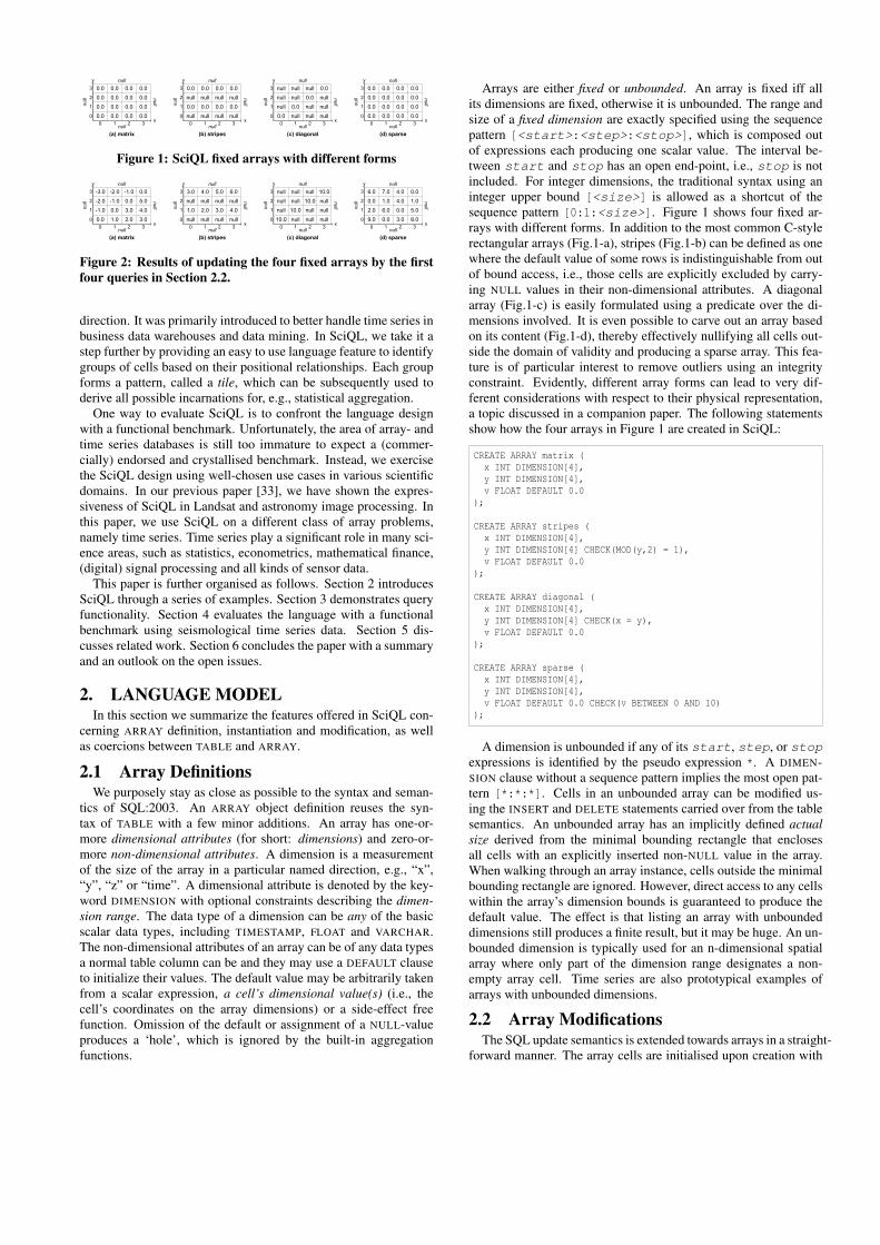
Figure 2: Results of updating the four fixed arrays by the firstfour queries in Section 2.2.

direction. It was primarily introduced to better handle time series inbusiness data warehouses and data mining. In SciQL, we take it astep further by providing an easy to use language feature to identifygroups of cells based on their positional relationships. Each groupforms a pattern, called a tile, which can be subsequently used toderive all possible incarnations for, e.g., statistical aggregation.

One way to evaluate SciQL is to confront the language designwith a functional benchmark. Unfortunately, the area of array- andtime series databases is still too immature to expect a (commer-cially) endorsed and crystallised benchmark. Instead, we exercisethe SciQL design using well-chosen use cases in various scientificdomains. In our previous paper [33], we have shown the expres-siveness of SciQL in Landsat and astronomy image processing. Inthis paper, we use SciQL on a different class of array problems,namely time series. Time series play a significant role in many sci-ence areas, such as statistics, econometrics, mathematical finance,(digital) signal processing and all kinds of sensor data.

This paper is further organised as follows. Section 2 introducesSciQL through a series of examples. Section 3 demonstrates queryfunctionality. Section 4 evaluates the language with a functionalbenchmark using seismological time series data. Section 5 dis-cusses related work. Section 6 concludes the paper with a summaryand an outlook on the open issues.

2. LANGUAGE MODELIn this section we summarize the features offered in SciQL con-

cerning ARRAY definition, instantiation and modification, as wellas coercions between TABLE and ARRAY.

2.1 Array DefinitionsWe purposely stay as close as possible to the syntax and seman-

tics of SQL:2003. An ARRAY object definition reuses the syn-tax of TABLE with a few minor additions. An array has one-or-more dimensional attributes (for short: dimensions) and zero-or-more non-dimensional attributes. A dimension is a measurementof the size of the array in a particular named direction, e.g., “x”,“y”, “z” or “time”. A dimensional attribute is denoted by the key-word DIMENSION with optional constraints describing the dimen-sion range. The data type of a dimension can be any of the basicscalar data types, including TIMESTAMP, FLOAT and VARCHAR.The non-dimensional attributes of an array can be of any data typesa normal table column can be and they may use a DEFAULT clauseto initialize their values. The default value may be arbitrarily takenfrom a scalar expression, a cell’s dimensional value(s) (i.e., thecell’s coordinates on the array dimensions) or a side-effect freefunction. Omission of the default or assignment of a NULL-valueproduces a ‘hole’, which is ignored by the built-in aggregationfunctions.

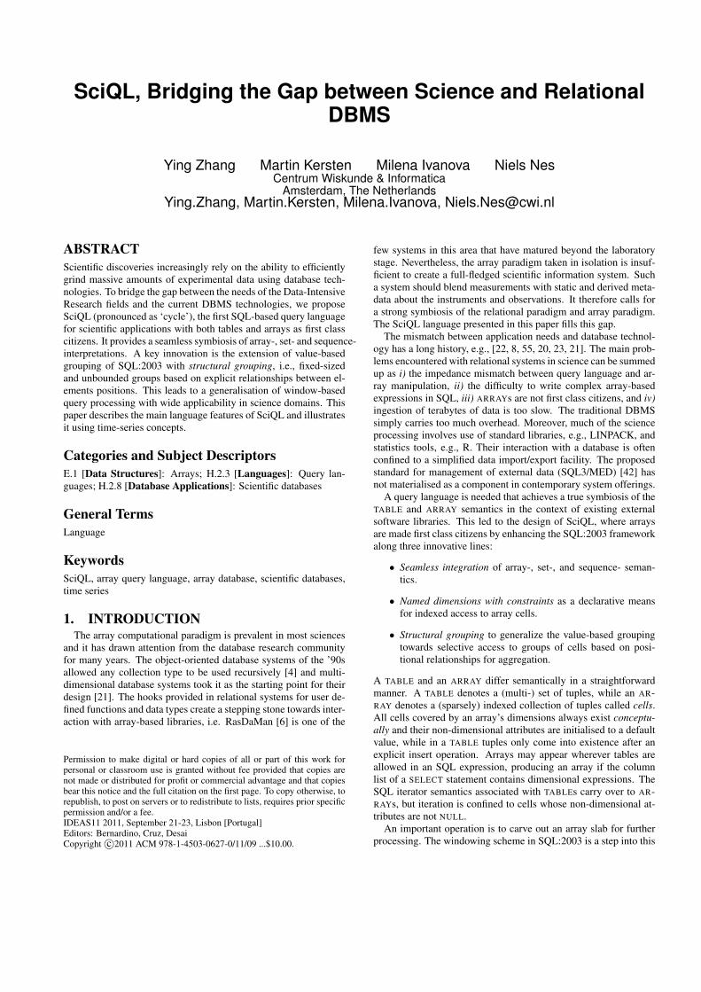
Arrays are either fixed or unbounded. An array is fixed iff allits dimensions are fixed, otherwise it is unbounded. The range andsize of a fixed dimension are exactly specified using the sequencepattern [<start>:<step>:<stop>], which is composed outof expressions each producing one scalar value. The interval be-tween start and stop has an open end-point, i.e., stop is notincluded. For integer dimensions, the traditional syntax using aninteger upper bound [<size>] is allowed as a shortcut of thesequence pattern [0:1:<size>]. Figure 1 shows four fixed ar-rays with different forms. In addition to the most common C-stylerectangular arrays (Fig.1-a), stripes (Fig.1-b) can be defined as onewhere the default value of some rows is indistinguishable from outof bound access, i.e., those cells are explicitly excluded by carry-ing NULL values in their non-dimensional attributes. A diagonalarray (Fig.1-c) is easily formulated using a predicate over the di-mensions involved. It is even possible to carve out an array basedon its content (Fig.1-d), thereby effectively nullifying all cells out-side the domain of validity and producing a sparse array. This fea-ture is of particular interest to remove outliers using an integrityconstraint. Evidently, different array forms can lead to very dif-ferent considerations with respect to their physical representation,a topic discussed in a companion paper. The following statementsshow how the four arrays in Figure 1 are created in SciQL:

CREATE ARRAY matrix (x INT DIMENSION[4],y INT DIMENSION[4],v FLOAT DEFAULT 0.0

);

CREATE ARRAY stripes (x INT DIMENSION[4],y INT DIMENSION[4] CHECK(MOD(y,2) = 1),v FLOAT DEFAULT 0.0

);

CREATE ARRAY diagonal (x INT DIMENSION[4],y INT DIMENSION[4] CHECK(x = y),v FLOAT DEFAULT 0.0

);

CREATE ARRAY sparse (x INT DIMENSION[4],y INT DIMENSION[4],v FLOAT DEFAULT 0.0 CHECK(v BETWEEN 0 AND 10)

);

A dimension is unbounded if any of its start, step, or stopexpressions is identified by the pseudo expression *. A DIMEN-SION clause without a sequence pattern implies the most open pat-tern [*:*:*]. Cells in an unbounded array can be modified us-ing the INSERT and DELETE statements carried over from the tablesemantics. An unbounded array has an implicitly defined actualsize derived from the minimal bounding rectangle that enclosesall cells with an explicitly inserted non-NULL value in the array.When walking through an array instance, cells outside the minimalbounding rectangle are ignored. However, direct access to any cellswithin the array’s dimension bounds is guaranteed to produce thedefault value. The effect is that listing an array with unboundeddimensions still produces a finite result, but it may be huge. An un-bounded dimension is typically used for an n-dimensional spatialarray where only part of the dimension range designates a non-empty array cell. Time series are also prototypical examples ofarrays with unbounded dimensions.

2.2 Array ModificationsThe SQL update semantics is extended towards arrays in a straight-

forward manner. The array cells are initialised upon creation with

the default values. A cell is given a new value through an ordinarySQL UPDATE statement. A dimension can be used as a bound vari-able, which takes on all its dimension values (i.e., valid values ofthis dimension) successively. A convenient shortcut is to combinemultiple updates into a single guarded statement. The evaluationorder ensures that the first predicate that holds dictates the cell val-ues. The refinement of the array matrix is shown in the first querybelow. The cells receive a zero only in the case x = y. The remain-ing queries demonstrate setting cell values in the arrays stripes,diagonal and sparse, respectively. The results are shown in Fig-ure 2.

UPDATE matrix SET v =CASE WHEN x > y THEN x + y WHEN x < y THEN x - y ELSE 0 END;

UPDATE stripes SET v = x + y;

UPDATE diagonal SET v = v + 10;

UPDATE sparse SET v = MOD(RAND(),16);

Assignment of a NULL value to an array cell leads to a ‘hole’in the array, a place indistinguishable from the out of bounds area.Such assignments overrule any predefined DEFAULT clause attachedto the array definition. For convenience, the built-in array aggregateoperations SUM(), COUNT(), AVG(), MIN() and MAX() are appliedto non-NULL values only.

-3.0 -2.0 0.0 0.0-2.0 -1.0 5.0 0.0-1.0 0.0 4.0 0.00.0 1.0 3.0 0.00 1

null

null

null

null

0

1

2 3

2

3

x

y

Figure 3: Result of shift-ing and zero filling thelast column of matrix.

Arrays can also be updated us-ing INSERT and DELETE state-ments. Since all cells seman-tically exists by definition, bothoperations effectively turn intoupdate statements. The DELETEstatement creates holes by assign-ing a NULL value for all qualifiedcells. The INSERT statement sim-ply overwrites the cells at posi-tions as specified by the input columns with new values. Notethat although the UPDATE, INSERT and DELETE statements do notchange the existence of array cells, for unbounded arrays they mayresult in scaling the minimal bounding rectangle up/down. Thethree queries below together illustrate how to delete a column inthe array matrix where x = 2, then shift the remaining columns,and (manually) set the last column of matrix to its default value.In the second and third queries, the x and y dimensions of the arraymatrix are matched against the projection columns of the SELECTstatements. Cells at matching positions are assigned new values(see Figure 3).

DELETE FROM matrix WHERE x = 2;

INSERT INTO matrix SELECT x-1, y, v FROM matrix WHERE x > 2;

INSERT INTO matrix SELECT x, y, 0 FROM matrix WHERE x = 3;

2.3 Array and Table CoercionsOne of the strong features of SciQL is to switch easily between

a TABLE and an ARRAY perspective. Any array is turned into acorresponding table by simply selecting its attributes. The dimen-sions then form a compound primary key. For example, the matrixdefined earlier becomes a table using the expression SELECT x,y, v FROM matrix or using a CAST operation like CAST(matrixAS TABLE). Note, that the semantics of an array leads to materi-alisation of all cells within the dimension bounds (or the minimalbounding rectangle for unbounded arrays), even if their values were

set to a non-NULL default. A selection excluding the user specifieddefault values may solve this problem.

An arbitrary table can be coerced into an array if the columnlist of the SELECT statement contains the dimension qualifiers ‘[’and ‘]’ around a projection column, i.e., [<expr>]. Here, the<expr> is a <column name> or a value expression. For in-stance, let mtable be the table produced by casting the array matrixto a table. It can be turned into an array by picking the columnsforming the primary key in the column list as follows: SELECT[x], [y], v FROM mtable, or using the reverse cast operationCAST(mtable AS ARRAY(x,y)). The result is an unbounded ar-ray with actual size derived from the dimension column expressions[x] and [y]. The default values of all non-dimensional attributesare inherited from the default values in the original table.

3. QUERY MODELFrom a query’s perspective, querying a TABLE and an ARRAY

are much alike. In both cases elements are selected based on pred-icates, joins, and groupings. The result of any query expression isa table unless the column list contains the dimension qualifiers (‘[’and ‘]’). A novel way to use GROUP BY, called tiling, is introducedto improve structure based querying.

3.1 Cell Selections

SELECT x, y, v FROM matrix WHERE v >2;

SELECT [x], [y], v FROM matrix WHERE v >2;

SELECT [T.k], [y], v FROM matrix JOIN T ON matrix.x = T.i;

The examples above illustrate a few simple array queries. Thefirst query extracts values from the array matrix into a table. Thesecond one constructs a sparse array from the selection, whose di-mensional properties are inherited from the result set. The dimen-sion qualifiers introduce a new dimension range, i.e., a minimalbounding box is derived from the result set, such that the answersfall within its bounds. The last query shows how elements of inter-est can be obtained from both arrays and tables using an ordinaryjoin expression. It assumes a table T with two (or more) columns,where the column i is of a numeric type and the column k may be ofany scalar type. The expression extracts the subarray from matrixand sets the bounds to the smallest enclosing bounding box definedby the values of the columns T.k and y. The actual bounds of anarray can always be obtained from the built-in functions MIN() andMAX() over the dimensions.

3.2 Array SlicingAn ARRAY object can be considered an array of records in pro-

gramming language terms. Therefore, the language supports po-sitional index access conforming to the order the dimensions areintroduced in the array definition. All attributes (dimensional andnon-dimensional) of interest should be explicitly identified. A rangepattern, borrowed from the programming language arena, supportseasy slicing over individual dimensions using the aforementionedsequence pattern [<start>:<step>:<stop>]. The range pat-tern is allowed in both the FROM and GROUP BY clauses. To illus-trate this, we show a few slicing expressions over the arrays definedearlier (results are computed based on Fig. 2-a).

SELECT * FROM matrix[3][2];-- yields: (3, 2, 5.0)

SELECT v FROM matrix[*][1:3];-- yields: (-1.0), (-2.0), (0.0), (-1.0), (3.0), (0.0),(4.0),(5.0)

SELECT v FROM matrix[0:2:4][0:2:4];-- yields: (0.0), (-2.0), (2.0), (0.0)

The SQL UPDATE statement is extended to take array expres-sions directly. This leads to a more convenient and compact nota-tion in many situations. The bounds of the subarray are specified bya sequence pattern of literals. Again, a sequence of updates act asa guarded function. The array dimensions are used as bound vari-ables that run over all valid dimension values. This is illustratedusing the queries below:

UPDATE matrix SET matrix[0:2][*].v = v * 1.19;

UPDATE matrix SET matrix[x][*].v =CASE WHEN v < 0 THEN x WHEN v >10 THEN 10 * x ELSE 0 END;

3.3 Array ViewsA common case is to embed an array into a larger one, such that

a zero initialised bounding border is created, or to shift a vector be-fore moving averages are calculated. To avoid possible significantdata movements, the array VIEW constructor can be used instead.The first two queries below illustrate an embedding, i.e., to trans-pose and shift an array, respectively. In the SELECT clause, the xand y columns are used to identify the cells in the vmatrix to beupdated. The last example illustrates how the aforementioned ex-ample of shift with zero fill of a column (see Section 2.2, secondquery group) can be modelled as a view. Note that the results ofall SELECT statements in the examples below are tables, thus in thethird query, the ordinary SQL UNION semantics applies.

CREATE VIEW ARRAY vmatrix (x INT DIMENSION[-1:1:5],y INT DIMENSION[-1:1:5],w FLOAT DEFAULT 0.0

) ASSELECT y, x, v FROM matrix;

CREATE VIEW ARRAY vector (x INT DIMENSION[-1:1:5],w FLOAT DEFAULT 0.0

) ASSELECT A.x, (A.v+B.v)/2FROM matrix AS A JOIN (SELECT x+1 AS x, v FROM matrix) AS B

ON A.x = B.x;

CREATE VIEW ARRAY vmatrix2 (x INT DIMENSION[-1:1:5],y INT DIMENSION[-1:1:5],w FLOAT DEFAULT 0.0

) ASSELECT x, y, v FROM matrix WHERE x < 2 UNIONSELECT x-1, y, v FROM matrix WHERE x > 2 UNIONSELECT x, y, 0.0 FROM matrix WHERE x = 3;

3.4 Aggregate TilingA key operation in science applications is to perform statistics

on groups. They are commonly identified by an attribute or ex-pression list in a GROUP BY clause. This value-based grouping canbe extended to structural grouping for ARRAYs in a natural way.Large arrays are often broken into smaller pieces before being ag-gregated or overlaid with a structure to calculate, e.g., a Gaussiankernel function. SciQL supports fine-grained control over break-ing an array into possibly overlapping tiles using a slight variationof the SQL GROUP BY clause semantics. Therefore, the attributelist is replaced by a parametrised series of array elements, calledtiles. Tiling starts with an anchor point identified by its dimensionalvalue(s), which is extended with a list of cell denotations relative

(a)

0.6 0.7 0.4 0.20.3 0.1 0.4 0.10.2 0.6 0.7 0.50.9 0.2 0.3 0.80 1

null

null

null

null

0

1

2 3

2

3

x

y

Anchor point(b)

0.6 0.7 0.4 0.20.3 0.1 0.4 0.10.2 0.6 0.7 0.50.9 0.2 0.3 0.80 1

null

null

null

null

0

1

2 3

2

3

x

y

Anchor point(c)

0.6 0.7 0.4 0.20.3 0.1 0.4 0.10.2 0.6 0.7 0.50.9 0.2 0.3 0.80 1

null

null

null

0

1

2 3

2

3

x

y

Anchor point null

(d)

0.6 0.7 0.4 0.20.3 0.1 0.4 0.10.2 0.6 0.7 0.50.9 0.2 0.3 0.80 1

null

null

null

null

0

1

2 3

2

3

x

y Anchor point

Figure 4: SciQL Array Tiling

(a)

0.650 0.550 0.300 0.200

0.425 0.400 0.275 0.150

0.300 0.450 0.425 0.300

0.475 0.450 0.575 0.650

0 1

null

null

null

null

0

1

2 3

2

3

x

y

(b)

null null null null

0.425 null 0.275 null

null null null null

0.475 null 0.575 null

0 1

null

null

null

null

0

1

2 3

2

3

x

y

(c)

0.450 0.425 0.400 0.275

0.250 0.300 0.450 0.425

0.550 0.475 0.450 0.575

0.900 0.550 0.250 0.550

0 1

null

null

null

null

0

1

2 3

2

3

x

y

(d)

null 0.425 null

null null null

0.360 null null

0 1

null

null

null

null

0

1

2 3

2

3

x

y

Figure 5: Results of computing AVG() over the tiles.

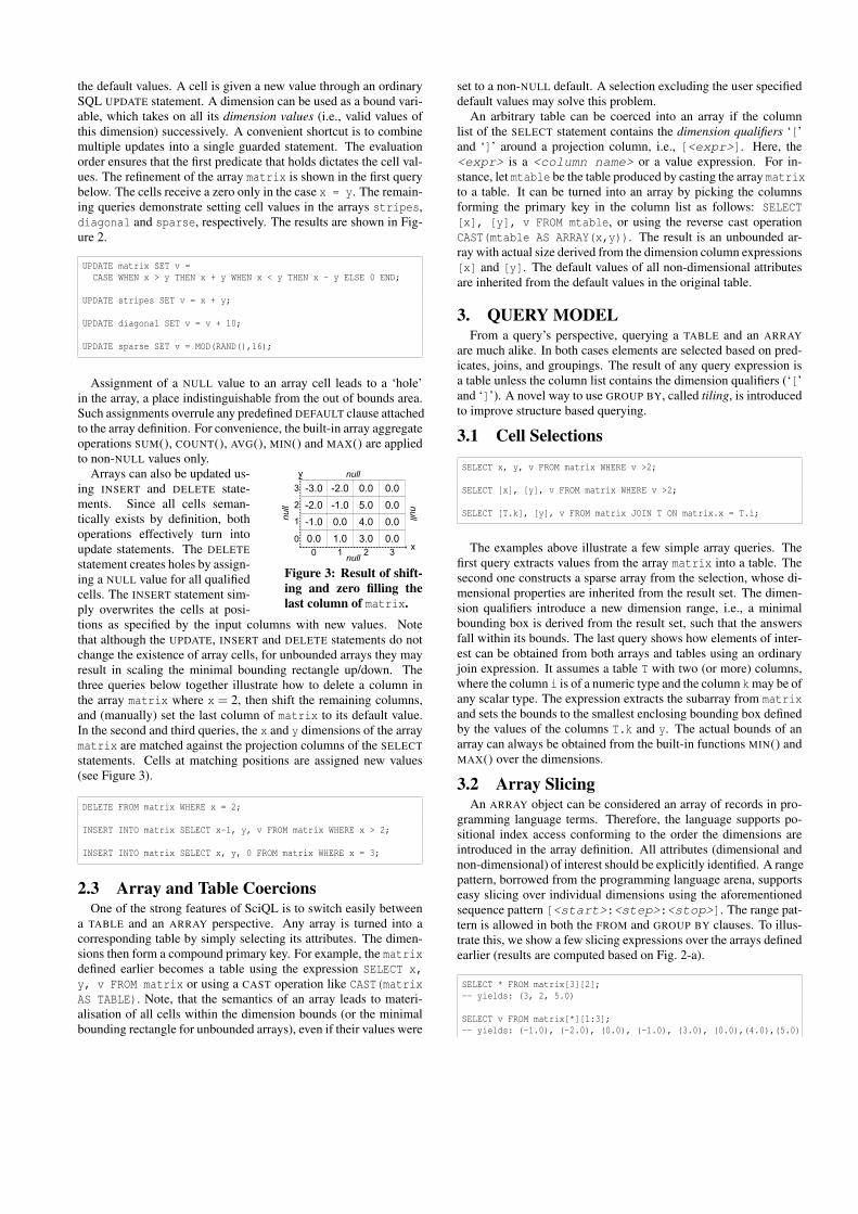
to the anchor point. The value derived from a group aggregation isassociated with the dimensional value(s) of the anchor point.

Consider a 4× 4 matrix and tiling it with a 2× 2 matrix by ex-tending the anchor point matrix[x][y] with structure elementsmatrix[x+1][y], matrix[x][y+1], and matrix[x+1][y+1]. Thetiling operation performs a grouping for every valid anchor pointon the actual array dimensions. Figure 4-a shows the first four tilescreated. The individual elements of a group need not belong to thedomain of the array dimensions, but then their values are assumedto be the outer NULL value, which are ignored in the statistical ag-gregate operations. This way we break the matrix array into 16overlapping tiles. The number can be reduced by explicitly callingfor DISTINCT tiles. This leads to considering each cell for one tileonly, leaving a hole behind for the next candidate tile. Furthermore,in this case all tiles with holes do not participate in the result set.This means that for irregularly formed tiles there is no guaranteethat all array cells are taking part in the grouping. The dimensionrange sequence pattern can be used to concisely define all valuesof interest. The following queries create the tiles on matrix as de-picted in Figure 4 (in the order from left to right). The query resultsare shown in Figure 5.

SELECT [x], [y], AVG(v)FROM matrixGROUP BY matrix[x:x+2][y:y+2];

SELECT [x], [y], AVG(v)FROM matrixGROUP BY DISTINCT matrix[x:x+2][y:y+2];

SELECT [x], [y], AVG(v)FROM matrixGROUP BY matrix[x-1:x+1][y-1:y+1];

SELECT [x], [y], AVG(v)FROM matrix[1:*][1:*]GROUP BY DISTINCT matrix[x][y], matrix[x-1][y], matrix[x+1][y],

matrix[x][y-1], matrix[x][y+1];

A recurring operation is to derive check sums over array slabs.In SciQL this can be achieved with a simple tiling on, e.g., the xdimension. In this case, the anchor point is the value of x. Forexample:

SELECT [x], SUM(v) FROM matrix GROUP BY matrix[x][*];

A discrete convolution operation is only slightly more complex.For, consider each element to be replaced by the average of itsneighboring elements. The extended matrix vmatrix is used tocalculate the convolution, because it ensures a zero value for allboundary elements. The aggregates outside the bounds [0:4][0:4]are not calculated by using an array slicing in the FROM clause.

SELECT [x], [y], AVG(v)FROM vmatrix[0:4][0:4]GROUP BY vmatrix[x-1:1:x+2][y-1:1:y+2];

Value based selection and structure based selection can be com-bined. An example is the nearest neighbor search, where the struc-ture dictates the context over which a metric function is evaluated.Most systems dealing with feature vectors deploy a default metric,e.g., the Euclidean distance. The example below assumes such adistance function that takes an argument ?V as the reference vector.It generates a listing of all columns with the distance from the refer-ence vector. Ranking the result produces the K-nearest neighbors.

SELECT x, distance(matrix, ?V) AS distFROM matrixGROUP BY matrix[x][*] ORDER BY dist LIMIT 10;

Using the dimension values in the grouping clause permits complexstructures to be defined. It generalises the SQL:2003 windowingfunctions, which are limited to aggregations over sliding windowswith static bounds and shift count over a sequence. The SciQL ap-proach can be generalised to support the equivalent of mask-basedtile selections. For this we simply need a table with dimension val-ues, which are used within the GROUP BY clause as a pattern tosearch for.

4. TIME SERIES DATA PROCESSINGAfter introducing the main features of SciQL, we continue with

illustrating its expressiveness as a time series language. Generallyspeaking, a time series is a sequence of data points with each pointattached a time stamp. A time series can be regular or irregular.The data points in a regular time series are measured at successivetimes spaced at uniform time intervals. In the sciences, sensor data(e.g., temperature, ground motion and strain gauges) is often a reg-ular time series, as it comes in as a continuous stream at a fixedrate. An irregular time series contains data points at successivetimes spaced at arbitrary time intervals. Sensor data with gaps isan irregular time series, in which the gaps typically indicate mal-functioning sensors. In the time series domain there does not exista standardised functional test of expressiveness. Since the primarytarget of SciQL is the scientific domains, we take the data fromseismology (an important scientific domain with a huge amount oftime series data) as a yardstick. In this section, we first discuss howtime series are supported by SciQL. Then we demonstrate how thetypical operations of seismic signal processing can be easily andconcisely phrased in SciQL.

4.1 Time Series

4.1.1 Fixed Time SeriesIf experiments are conducted at regular intervals, it is helpful to

represent them as arrays indexed by the time stamps with a fixedstride. The SciQL language constructs allow for easy subsequentmanipulations, such as interpolation and computing moving aver-ages, without the need to resort to self-joins. The following queryshows how SciQL is turned into a time series supporting languageby simply choosing a temporal domain for at least one dimension:

CREATE ARRAY ts1 (time TIMESTAMP DIMENSION[TIMESTAMP ‘2011-01-01 09:00:00’ :

INTERVAL ‘1’ MINUTE :TIMESTAMP ‘2011-01-01 10:00:00’],

data FLOAT DEFAULT 0.0);

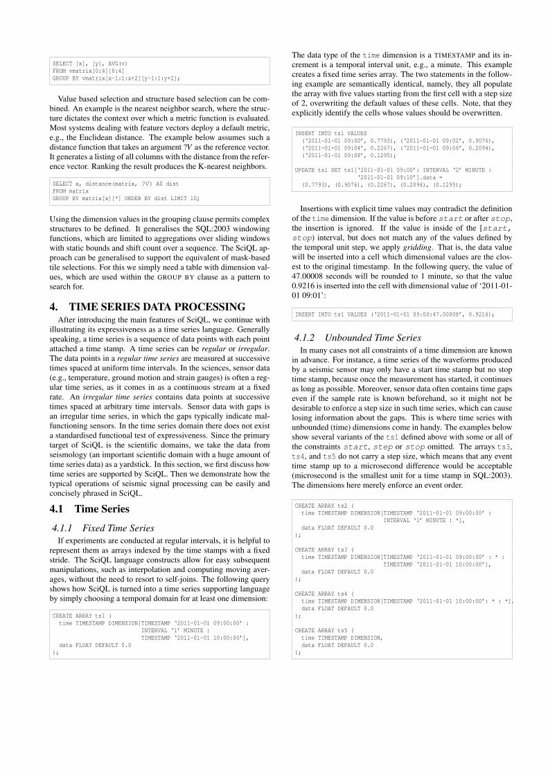
The data type of the time dimension is a TIMESTAMP and its in-crement is a temporal interval unit, e.g., a minute. This examplecreates a fixed time series array. The two statements in the follow-ing example are semantically identical, namely, they all populatethe array with five values starting from the first cell with a step sizeof 2, overwriting the default values of these cells. Note, that theyexplicitly identify the cells whose values should be overwritten.

INSERT INTO ts1 VALUES(‘2011-01-01 09:00’, 0.7793), (‘2011-01-01 09:02’, 0.9076),(‘2011-01-01 09:04’, 0.2267), (‘2011-01-01 09:06’, 0.2094),(‘2011-01-01 09:08’, 0.1295);

UPDATE ts1 SET ts1[‘2011-01-01 09:00’: INTERVAL ‘2’ MINUTE :‘2011-01-01 09:10’].data =

(0.7793), (0.9076), (0.2267), (0.2094), (0.1295);

Insertions with explicit time values may contradict the definitionof the time dimension. If the value is before start or after stop,the insertion is ignored. If the value is inside of the [start,stop) interval, but does not match any of the values defined bythe temporal unit step, we apply gridding. That is, the data valuewill be inserted into a cell which dimensional values are the clos-est to the original timestamp. In the following query, the value of47.00008 seconds will be rounded to 1 minute, so that the value0.9216 is inserted into the cell with dimensional value of ‘2011-01-01 09:01’:

INSERT INTO ts1 VALUES (‘2011-01-01 09:00:47.00008’, 0.9216);

4.1.2 Unbounded Time SeriesIn many cases not all constraints of a time dimension are known

in advance. For instance, a time series of the waveforms producedby a seismic sensor may only have a start time stamp but no stoptime stamp, because once the measurement has started, it continuesas long as possible. Moreover, sensor data often contains time gapseven if the sample rate is known beforehand, so it might not bedesirable to enforce a step size in such time series, which can causelosing information about the gaps. This is where time series withunbounded (time) dimensions come in handy. The examples belowshow several variants of the ts1 defined above with some or all ofthe constraints start, step or stop omitted. The arrays ts3,ts4, and ts5 do not carry a step size, which means that any eventtime stamp up to a microsecond difference would be acceptable(microsecond is the smallest unit for a time stamp in SQL:2003).The dimensions here merely enforce an event order.

CREATE ARRAY ts2 (time TIMESTAMP DIMENSION[TIMESTAMP ‘2011-01-01 09:00:00’ :

INTERVAL ‘1’ MINUTE : *],data FLOAT DEFAULT 0.0

);

CREATE ARRAY ts3 (time TIMESTAMP DIMENSION[TIMESTAMP ‘2011-01-01 09:00:00’ : * :

TIMESTAMP ‘2011-01-01 10:00:00’],data FLOAT DEFAULT 0.0

);

CREATE ARRAY ts4 (time TIMESTAMP DIMENSION[TIMESTAMP ‘2011-01-01 10:00:00’: * : *],data FLOAT DEFAULT 0.0

);

CREATE ARRAY ts5 (time TIMESTAMP DIMENSION,data FLOAT DEFAULT 0.0

);

Compared with fixed time series, inserting values into an un-bounded time series without explicitly specifying the cell indiceshas several semantic differences. Basically, the values can be in-serted at any positions satisfying the partial constraints of the timedimension in the array definition, as long as the relative order amongthe values is preserved. However, this operation can be made moredeterministic by using the available constraints. Unbounded timeseries can be divided into the following classes, based on the ab-sent dimension constraint(s): i) one end of the dimension range(i.e., start or stop); ii) both ends of the dimension range; iii)the step size; iv) one end of the dimension range and the step size;and v) all constraints. The first class is easy to handle. Consider thequery:

INSERT INTO ts2 VALUES(0.7793), (0.9076), (0.2267), (0.2094), (0.1295);

Since the array ts2 has a start and step for its time dimen-sion, the values are inserted into the first five cells of the array (ifthe start was omitted, the last five cells are chosen), i.e., at thetimestamps ‘2011-01-01 09:00’, ‘2011-01-01 09:01’, . . . , ‘2011-01-01 09:04’, overwriting any existing values at these positions. Ifboth ends of the dimension ranges are omitted (class ii)), we takethe current time now(), rounded to the granularity of the step size,as the starting position for insertions. When the step size is omitted(class iii)), we use the smallest unit of the dimension data type asthe default step size. In case of timestamp, it is the microsecond.Thus, the query:

INSERT INTO ts3 VALUES(0.7793), (0.9076), (0.2267), (0.2094), (0.1295);

produces the time series ((‘2011-01-01 09:00:00.000000’, 0.7793),. . . , (‘2011-01-01 09:00:00.000004’, 0.1295)). To handle the un-bounded time series of the classes iv) and v), we combine the rulesused for the first three classes. For instance, to handle the query:

INSERT INTO ts5 VALUES(0.7793), (0.9076), (0.2267), (0.2094), (0.1295);

we take the value of now() as the start position and microsecond asthe step size.

4.1.3 InterpolationApplications often assume values at regular time intervals, while

the available measurement time series may have gaps of missingvalues or values taken at irregular time intervals. In such cases in-terpolation can be used to provide approximate values at regulartime steps. Consider the irregular time series ts4 set by the follow-ing query:

INSERT INTO ts4 VALUES(‘2011-01-01 09:00’, 0.28), (‘2011-01-01 09:02’, 0.36),(‘2011-01-01 09:05’, 0.52);

The interpolation can be formulated in SciQL as follows. First,we create a fixed time series with the desired regular step, for in-stance 1 minute:

CREATE ARRAY heartbeat (time TIMESTAMP DIMENSION[TIMESTAMP ‘2011-01-01 09:00’ :

INTERVAL ‘1’ MINUTE :TIMESTAMP ‘2011-01-01 10:00’],

data FLOAT DEFAULT NULL);

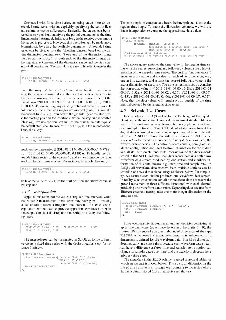
The next step is to compute and insert the interpolated values at theregular time steps. To make the discussion concrete, we will uselinear interpolation to compute the approximate data values:

INSERT INTO heartbeatSELECT hb.time,

irr.data + (hb.time - irr.time) *(irr[NEXT(irr, irr.time)].data - irr.data) /(NEXT(irr, irr.time) - irr.time)

FROM heartbeat AS hb, ts4 AS irrWHERE hb.time >= irr.time AND hb.time <= NEXT(irr, irr.time);

The above query matches the time value in the regular time se-ries with the nearest preceding and following values in the time di-mension of the irregular time series. The built-in function NEXT()takes an array name and a value for each of its dimension, onlyone in this example, and returns the nearest following value in themajor dimension of the array. The time series heartbeat containsthe non-NULL values: ((‘2011-01-01 09:00’, 0.28), (‘2011-01-0109:01’, 0.32), (‘2011-01-01 09:02’, 0.36), (‘2011-01-01 09:03’,0.413), (‘2011-01-01 09:04’, 0.466), (‘2011-01-01 09:05’, 0.52)).Note, that the data values will remain NULL outside of the timeinterval covered by the irregular time series.

4.2 Seismic Use CasesIn seismology, SEED (Standard for the Exchange of Earthquake

Data) [48] is the most widelyÂaused international standard file for-mat for the exchange of waveform data among global broadbandseismograph networks. The SEED standard defines a format fordigital data measured at one point in space and at equal intervalsof time. A SEED volume consists of a number of ASCII con-trol headers followed by a number of binary data records, i.e., thewaveform time series. The control headers contain, among others,all the configuration and identification information for the stationand all its instruments, and meta information of the data recordsstored in this SEED volume. Each data record contains both a rawwaveform data stream produced by one station and auxiliary in-formation of this data stream, e.g., start time and sample rate. InSciQL, all waveform data streams from multiple stations can bestored in one two-dimensional array, as shown below. For simplic-ity, we assume each station produces one waveform data stream.In reality, a seismic station contains three channels (to measure theground movement in three different directions) with each channelproducing one waveform data stream. Separating data streams fromdifferent channels merely adds one more integer dimension in thearray MSeed.

CREATE ARRAY MSeed (station VARCHAR(5) DIMENSION[‘0’ : * : ‘ZZZZZ’],time TIMESTAMP DIMENSION,data FLOAT

);

Since each seismic station has an unique identifier consisting ofup to five characters (upper case letters and the digits 0 – 9), thestation IDs is denoted using an unbounded dimension of the typeVARCHAR, which uses the lexical order. Finally, an unbounded timedimension is defined for the waveform data. The time dimensiondoes not carry any constraints, because each waveform data streamcan have a different start/stop time and sample rate, a station canchange its sampling rate over time, and the waveform data can havearbitrary time gaps.

The meta data in the SEED volume is stored in normal tables, ofwhich an excerpt is shown below. The station dimension in theMSeed array also acts as foreign keys pointing to the tables wherethe meta data is stored (not all attributes are shown):

(1)n = -3m = 3

f ★ g = 2

(2)n = -2

m = 2, 3f ★ g = 16

(3)n = -1

m = 1, 2, 3f ★ g = 47

(4)n = 0

m = 0, 1, 2f ★ g = 61

(5)n = 1

m = 0, 1f ★ g = 41

(6)n = 2m = 0

f ★ g = 28

f 4 3 6 2

g 1 5 7

f 4 3 6 2

g 1 5 7

f 4 3 6 2

g 1 5 7

f 4 3 6 2

g 1 5 7

f 4 3 6 2

g 1 5 7

f 4 3 6 2

g 1 5 7

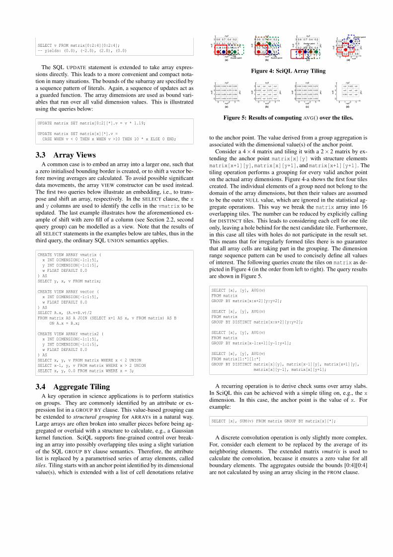
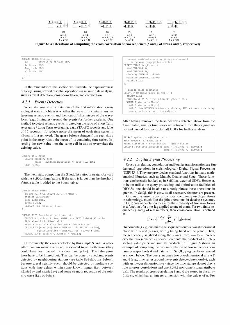
Figure 6: All iterations of computing the cross-correlation of two sequences f and g of sizes 4 and 3, respectively

CREATE TABLE Station (id VARCHAR(5) PRIMARY KEY,latitude DEC,longitude DEC,altitude DEC,...

);

In the remainder of this section we illustrate the expressivenessof SciQL using several essential operations in seismic data analysis,such as event detection, cross-correlation, and convolution.

4.2.1 Events DetectionWhen studying seismic data, one of the first information a seis-

mologist wants to obtain is whether the waveform contains any in-teresting seismic events, and then cut off short pieces of the wave-form (e.g., 3 minutes) around the events for further analysis. Onemethod to detect seismic events is based on the ratio of Short TermAveraging / Long Term Averaging, e.g., STA of 2 seconds and LTAof 15 seconds. To reduce noise the mean of each time series inMSeed is first removed. The query below subtracts from each datapoint in the array MSeed the mean of its containing time series. In-serting the new value into the same cell in MSeed overwrites theexisting value.

INSERT INTO MSeedSELECT station, time,

(data - AVG(MSeed[station][*].data)) AS dataFROM MSeed;

The next step, computing the STA/LTA ratio, is straightforwardwith the SciQL tiling feature. If the ratio is larger than the thresholddelta, a tuple is added to the Event table:

CREATE TABLE Event (id INT NOT NULL UNIQUE AUTO_INCREMENT,station VARCHAR(5),time TIMESTAMP,ratio FLOAT,PRIMARY KEY (station, time)

);

INSERT INTO Event(station, time, ratio)SELECT A.station, A.time, AVG(A.data)/AVG(B.data) AS ratioFROM MSeed AS A, MSeed AS BWHERE A.station = B.station AND A.time = B.timeGROUP BY A[station][time - INTERVAL ‘2’ SECOND : time],

B[station][time - INTERVAL ‘15’ SECOND : time]HAVING AVG(A.data)/AVG(B.data) > ?delta;

Unfortunately, the events detected by this simple STA/LTA algo-rithm contain many events not associated to an earthquake (theycould have been caused by a cow passing by). The false posi-tives have to be filtered out. This can be done by checking eventsdetected by neighbouring stations (see table Neighbours below),because a real seismic event should be detected by multiple sta-tions with time delays within some known ranges (i.e., betweenmindelay and maxdelay) and some strength reduction of the seis-mic wave (i.e., weight).

-- detect isolated errors by direct environment-- using wave propagation staticsCREATE TABLE Neighbours (

sta1 VARCHAR(5),sta2 VARCHAR(5),mindelay INTERVAL SECOND,maxdelay INTERVAL SECOND,weight FLOAT

);

-- detect false positives:DELETE FROM Event WHERE id NOT IN (

SELECT A.idFROM Event AS A, Event AS B, Neighbours AS NWHERE A.station = N.sta1

AND B.station = N.sta2AND B.time BETWEEN A.time + N.mindelay AND A.time + N.maxdelayAND A.ratio > B.ratio * N.weight);

After having removed the false positives detected above from theEvent table, smaller time series are retrieved from the original ar-ray and passed to some (external) UDFs for further analysis:

SELECT myfunction(A[station].*)FROM MSeed AS A, Event AS BWHERE A.station = B.station AND A.time = B.timeGROUP BY DISTINCT A[station][time - INTERVAL ‘1’ MINUTE :

time + INTERVAL ‘2’ MINUTE];

4.2.2 Digital Signal ProcessingCross-correlation, convolution and Fourier transformation are fun-

damental operations in (seismological) Digital Signal Processing(DSP) [54]. They are provided as standard functions in many math-ematical libraries, such as Matlab, Octave and Sage. Those func-tions can be easily hooked up in SciQL as external UDFs. However,to better utilise the query processing and optimisation facilities ofDBMSs, one should be able to directly phrase these operations inqueries. In SciQL this is easy, as all necessary features are present.

Cross-correlation is one of the most commonly used operationsin seismology, much like the join operations in database systems.In DSP, cross-correlation measures the similarity of two waveformsas a function of a time-lag applied to one of them. For two finite se-quences f and g of real numbers, their cross-correlation is definedas:

( f ?g)[n]de f=

∞

∑m=−∞

f [n]g[n+m]

To compute f ?g, one maps the sequences onto a two-dimensionalplane with x- and y- axes, with g being fixed on the plane. Then,the sequence f is slided along the x axes from −∞ to ∞. Wher-ever the two sequences intersect, compute the product of all inter-secting value pairs and sum all products up. Figure 6 shows anexample of computing the cross-correlation of two sequences con-taining respectively 4 and 3 items. In SciQL, f ?g can be expressedas shown below. The query assumes two one-dimensional arrays Fand G (e.g., time series around the events detected previously), eachwith an integer dimension pos (since the time stamps do not play arole in cross-correlation) and one FLOAT non-dimensional attributeval. The results of cross-correlating F and G are stored in the arrayCrCorr, which has an integer dimension with the values of n. For

each cell of CrCorr, the query takes the intersecting slices of F andG (in the GROUP BY clause) to compute the products and sum. Thebuilt-in functions MIN() and MAX() return the smaller/larger valueof its two parameters, which are used to prevent array slicing fromgoing out of the dimension bounds.

DECLARE fmin INT, fmax INT, fcnt INT, gmin INT, gcnt INT, n INT;SET fmin = SELECT MIN(pos) FROM F;SET fmax = SELECT MAX(pos) FROM F;SET fcnt = SELECT COUNT(*) FROM F;SET gmin = SELECT MIN(pos) FROM G;SET gcnt = SELECT COUNT(*) FROM G;SET n = -fmax;

CREATE ARRAY CrCorr (idx INT DIMENSION[n:1:gcnt],val FLOAT DEFAULT 0.0

);

INSERT INTO CrCorrSELECT C.idx, SUM(F.val * G.val)FROM F, G, CrCorr AS CGROUP BY F[MAX(fmin, -C.idx) : MIN(fcnt, gcnt-C.idx)],

G[MAX(gmin, C.idx) : MIN(gcnt, fcnt+C.idx)];

Computing the convolution of two sequences f ∗ g is anotherimportant operation in seismology. It is used in, e.g., design andimplementation of Finite Impulse Response filters in DSP. Convo-lution differs from cross-correlation only in one step, namely, thesequence f is first reversed before it is slided. Sequence reversingin SciQL is captured by a slicing with negative step size, stored asan array view Fr. The following query computes the convolutionof F and G and stores the results in Conv (variables are borrowedfrom the cross-correlation example).

CREATE VIEW ARRAY Fr (pos INT DIMENSION[fmin:1:fmax],val FLOAT

) ASSELECT val FROM F[fmax:-1:fmin];

CREATE ARRAY Conv (idx INT DIMENSION[n:1:gcnt],val FLOAT DEFAULT 0.0

);

INSERT INTO ConvSELECT C.idx, SUM(Fr.val * G.val)FROM Fr, G, Conv AS CGROUP BY Fr[MAX(fmin, -C.idx) : MIN(fcnt, gcnt-C.idx)],

G[MAX(gmin, C.idx) : MIN(gcnt, fcnt+C.idx)];

The discrete Fourier transform (DFT) is a mathematical oper-ation that transforms a discrete sequence in the time domain intoits frequency domain representation. Since the output (sequence)of a DFT always contains complex numbers, a data type not sup-ported by SQL:2003, we discuss here how the real DFT can bewritten in SciQL. The real DFT is a version of the discrete Fouriertransform that uses real numbers to represent both the input andoutput signals. Given a sequence of N real numbers x[i], wherei = 0, · · · ,N − 1, the real DFT transforms it into two sequencesof N/2 real numbers ReX [k] and ImX [k], where k = 0, · · · ,N/2.ReX [k] and ImX [k] are computed as the following:

ReX [k] =N−1

∑i=0

x[i]cos(2πki/N) ImX [k] =−N−1

∑i=0

x[i]sin(2πki/N)

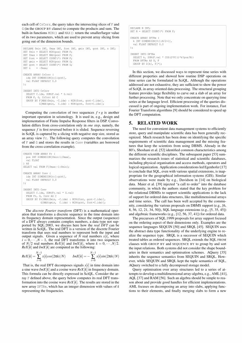
That is, the real DFT decomposes signals x[i] in time domain intoa sine wave ImX [k] and a cosine wave ReX [k] in frequency domain.This formula can be directly expressed in SciQL. Consider the ar-ray F defined above, the query below computes its real DFT trans-formation into the cosine wave ReX [k]. The results are stored in thenew array DFTRe, which has an integer dimension with values of krepresenting the frequencies.

DECLARE N INT;SET N = SELECT COUNT(*) FROM F;

CREATE ARRAY DFTRe (k INT DIMENSION[0:1:N/2+1],val FLOAT DEFAULT 0.0

);

INSERT INTO DFTReSELECT k, SUM(F.val * COS(2*PI()*k*pos/N))FROM DFTRe AS D, FGROUP BY D[k], F[*];

In this section, we discussed ways to represent time series withdifferent properties and showed how routine DSP operations ontime series can be formulated in SciQL. Although the operationsaddressed are not exhaustive, they are sufficient to show the powerof SciQL in array oriented data processing. The structural groupingfeature provides large flexibility to carve out a slab of an array forfurther processing. Note that we only concentrate on querying timeseries at the language level. Efficient processing of the queries dis-cussed is part of ongoing implementation work. For instance, FastFourier Transform algorithms [9] should be considered to speed upthe DFT computation.

5. RELATED WORKThe need for convenient data management systems to efficiently

store, query and manipulate scientific data has been generally rec-ognized. Much research has been done on identifying the specificrequirements of scientific data management and the missing fea-tures that keep the scientists from using DBMS. Already in the80’s, Shoshani et al. [52] identified common characteristics amongthe different scientific disciplines. The subsequent paper [53] sum-marizes the research issues of statistical and scientific databases,including physical organisation and access methods, operators andlogical organization. Application considerations led Egenhofer [17]to conclude that SQL, even with various spatial extensions, is inap-propriate for the geographical information systems (GIS). Similarobservations were made by e.g., Davidson in [14] on biologicaldata. Maier et al. [39] injected “a call to order” into the databasecommunity, in which the authors stated that the key problem forthe relational DBMSs to support scientific applications is the lackof support for ordered data structures, like multidimensional arraysand time series. The call has been well accepted by the commu-nity, considering the various proposals on DBMS support (e.g., [6,8, 56, 12, 21, 34, 50]), SQL language extensions (e.g., [5, 35, 45])and algebraic frameworks (e.g., [12, 56, 37, 41]) for ordered data.

The precursors of SQL:1999 proposals for array support focusedon the ordering aspect of their dimensions only. Examples are thesequence languages SEQUIN [50] and SRQL [45]. SEQUIN usesthe abstract data type functionality of the underlying engine to re-alize the sequence type. SRQL is a successor of SEQUIN whichtreated tables as ordered sequences. SRQL extends the SQL FROMclauses with GROUP BY and SEQUENCE BY to group by and sortthe input relations. Both systems did not consider the shape bound-aries in their semantics and optimisation schemes. AQuery [35]inherits the sequence semantics from SEQUIN and SRQL. How-ever, while SEQUIN and SRQL kept the tuple semantics of SQL,AQuery switched to a fully decomposed storage model.

Query optimisation over array structures led to a series of at-tempts to develop a multidimensional array-algebra, e.g., AML [41],AQL [37] and RAM [56]. Such an algebra should be simple to rea-son about and provide good handles for efficient implementations.AML focuses on decomposing an array into slabs, applying func-tions to their elements, and finally merging slabs to form a new

array. AQL is an algebraic language with low-level array manip-ulation primitives. Four array-related primitives (two for creation,one for subscripting and one for determining shapes) plus auxil-iary features, e.g., conditionals and arithmetic operations, allowapplication-specific array operations to be defined within AQL. Theuser specifies an algebraic tree with embedded UDF calls. NeitherAML nor AQL provides a declarative mechanism to define the or-der the queries manipulate data. Comparing with array algebras,SciQL has a much more intuitive approach where the user focuseson the final structure.

RAM [56] is a proposal for flexible representation of informationretrieval models in a single multidimensional array framework. Itintroduces an array algebra language on top of MonetDB [7] andis used as the “gluing layer” for DB+IR applications. RAM de-fines a set of basic array algebra operators, including MAP, APPLY,AGGREGATE, CONCAT, etc. Queries in RAM are compiled by thefront-end into an execution plan to be executed by the MonetDBkernel. RAM does not support a declarative language such as SQL.SRAM [12] is a following up of RAM that pays special attention toefficient storing and querying of sparse arrays in relational DBMS.

Despite the abundance of research effort, few systems can han-dle sizable arrays efficiently. A good example is RasDaMan [6],which is a domain-independent array DBMS for multidimensionalarrays of arbitrary size and structure. It has completely been de-signed in an object-oriented manner. It follows the classical two-tier client/server architecture with query processing done completelywithin the server. Arrays are decomposed into chunks, which formthe unit of storage and access. The chunks are stored as BLOBS,so (theoretically) it can be ported to any DBMS supporting BLOBs.The RasDaMan server acts as a middleware, mapping the array se-mantics to a simple “set of BLOB” semantics. RasDaMan providesan SQL-92 based query language RasQL [5] to manipulate rasterimages using foreign function implementations. It defines a com-pact set of operators, e.g., MARRAY creates an array and fills it byevaluating a given expression at each cell; CONDENSE aggregatescell values into one scalar value; SORT slices an array along one ofits axes and reorders the slices. RasQL queries are executed by theRasDaMan server, after the necessary BLOBs have been retrievedfrom the underlying DBMS.

The approaches taken by RAM and RasDaMan have a com-mon drawback: arrays are black boxes to the underlying DBMS.This means that RAM and RasDaMan cannot fully benefit fromthe query execution facilities provided by the underlying DBMS.Contrary, the underlying DBMS is not aware of the specific arrayproperties, missing opportunities for query optimization.

A recent attempt to develop an array database system from scratchis undertaken by the SciDB group [55]. Its mission is the closest toSciQL, namely, building an array DBMS with tailored features tofit exactly the need of the science community. The work of SciDBhas focused on an efficient distributed architecture for array queryprocessing ([13], [8]), in which arrays are vertically partitioned anddivided into overlapping chunks (or slabs). At the language level,SciDB (version 0.75) supports both a declarative Array Query Lan-guage (AQL) and an Array Functional Language (AFL) [46](notethat SciDB’s AQL is unrelated with the earlier work on the alge-braic language AQL [37]). AQL supports a subset of SQL featureswith extensions allowing creating arrays with named dimensions.Only integer typed dimensions are supported and the users shouldspecify how the array should be divided into chunks when creatingan array. Most array manipulation features are defined in the AFLby means of functional operators, e.g., SLICE, SUBSAMPLE, SJOIN,FILTER and APPLY. Compared with AQL and AFL, SciQL takeslanguage design a step further by proposing a seamless integration

with SQL:2003 syntax and semantics.Various database researchers have embarked on scientific ap-

plications that call for an array query language. PostgreSQL al-lows columns of a table to be defined as variable-length multidi-mensional array. Arrays of built-in type, enum type, compositetype and user-defined base type can all be created. Basic arith-metic operators on arrays and simple slicing, i.e., integer indexesalways increased by 1, are supported. Unfortunately, PostgreSQLhas followed the SQL standard to use anonymous dimensions, alimitation that has been disputed by the science community [47].AQuery [35] integrates table and array semantics into one kind ofordered entities arrables, a.k.o column store where the index iskept. An arrable’s ordering can be defined at creation time usingan ORDERED BY clause, which can be also altered per query, usingan ASSUMING ORDER clause. Array access is supported with a fewfunctions, e.g., first(<N>, <col>) and last(<N>,<col>).

Much research work has been done on time series data process-ing in the areas such as financial statistics [40, 18], (multimedia)image processing [30] and data mining [2, 30, 29]. Existing re-search work has been focused on algorithms for, e.g., similaritysearching (using distance algorithms) [10, 25, 57, 11, 16, 1], pat-tern detection or matching [44, 19, 59, 28, 24], classification [58,3, 36, 26], indexing [51, 31, 57] and compressing [18, 27, 32]. Ourwork at the language level is orthogonal to the existing techniquesfor, e.g., similarity searching, pattern matching and classification,while we might benefit from existing work on indexing and com-pressing when implementing SciQL. Nevertheless, many issues arestill left open. Very little work has been done on using DBMSs fortime series data processing, because it has been generally realisedthat scientific operations are difficult to be expressed in SQL andinefficient to evaluate [15, 49]. Existing techniques have in generalonly shown their usefulness for small time series [38]. [51] mightbe the only work that tries to tackle time series towards terabytes(up to 750GB). Thus, it is unknown how well the existing tech-niques will perform when dealing with terabytes and larger scaleof time series.

6. SUMMARY AND FUTURE WORKIn this paper we have introduced SciQL, a query language for

scientific applications and its use in querying time series. SciQLhas been designed to lower the entry fee for scientific applicationsto use a database system. The language stands on the shouldersof many earlier attempts. SciQL preserves the SQL:2003 flavorusing a minimal enhancements to the language syntax and seman-tics. Convenient syntax shortcuts are provided to express array ex-pressions using a conventional programming style. We illustratedthe needs for array-based query capabilities in the seismic wave-form data processing. The concise description in SciQL bringsrelational and array processing symbiosis one step closer to real-ity. Future work includes development of a formal semantics forthe array extensions, development of an adaptive storage schemeand exploration of the performance on functionally complete sci-ence applications. A prototype implementation of SciQL withinthe MonetDB [43] framework is being under development.

AcknowledgementsThe work reported here is partly funded by the EU-FP7-ICT projectsPlanetData (http://www.planet-data.eu/) and TELEIOS (http://www.earthobservatory.eu/).

7. REFERENCES[1] R. Agrawal et al. Fast similarity search in the presence of noise,

scaling, and translation in time-series databases. In VLDB ’95, pages490–501, San Francisco, CA, USA, 1995.

[2] C. M. Antunes and A. L. Oliveira. Temporal data mining: anoverview. In Proceedings of the EPIA 2001 Workshop on ArtificialIntelligence for Financial Time Series Analysis, 2001.

[3] A. J. Bagnall and G. J. Janacek. Clustering time series from armamodels with clipped data. In SIGKDD, pages 49–58, 2004.

[4] F. Bancilhon et al., editors. Building an Object-Oriented DatabaseSystem, The Story of O2. Morgan Kaufmann, 1992.

[5] P. Baumann. A database array algebra for spatio-temporal data andbeyond. In NGITS’2003, pages 76–93, 1999.

[6] P. Baumann et al. The multidimensional database systemRasDaMan. SIGMOD Rec., 27(2):575–577, 1998.

[7] P. Boncz. Monet: A Next-Generation DBMS Kernel ForQuery-Intensive Applications. PhD thesis, UVA, Amsterdam, TheNetherlands, May 2002.

[8] P. G. Brown. Overview of SciDB: large scale array storage,processing and analysis. In SIGMOD, pages 963–968, New York,NY, USA, 2010. ACM.

[9] C. Burrus, editor. Fast Fourier Transforms. Connexions, April 2009.http://cnx.org/content/col10550/1.21/.

[10] J. P. Caraça-Valente and I. López-Chavarrías. Discovering similarpatterns in time series. In SIGKDD, KDD ’00, pages 497–505, 2000.

[11] L. Chen, M. T. Özsu, and V. Oria. Robust and fast similarity searchfor moving object trajectories. In SIGMOD, pages 491–502, 2005.

[12] R. Cornacchia et al. Flexible and efficient IR using Array Databases.VLDB Journal, special issue on IR&DB integration, 17(1):151–168,January 2008.

[13] P. Cudre-Mauroux et al. A demonstration of SciDB: ascience-oriented DBMS. PVLDB, 2(2):1534–1537, 2009.

[14] S. B. Davidson. Tale of two cultures: Are there database researchissues in bioinformatics? In SSDBM’02, page 3, Washington, DC,USA, 2002.

[15] Dennis Shasha. Time series in finance: the array database approach.http://cs.nyu.edu/shasha/papers/jagtalk.html.

[16] H. Ding et al. Querying and mining of time series data: experimentalcomparison of representations and distance measures. Proc. VLDBEndow., 1:1542–1552, August 2008.

[17] M. J. Egenhofer. Why not SQL! International Journal ofGeographical Information Systems, 6(2):71–85, 1992.

[18] M. Falk et al. A First Course on Time Series Analysis. Chair ofStatistics, University of Würzburg, 2006.

[19] X. Ge and P. Smyth. Deformable markov model templates fortime-series pattern matching. In SIGKDD, pages 81–90, 2000.

[20] J. Gray, D. T. Liu, M. A. Nieto-Santisteban, A. S. Szalay, D. J.DeWitt, and G. Heber. Scientific data management in the comingdecade. SIGMOD Record, 34(4):34–41, 2005.

[21] M. Gyssens and L. V. S. Lakshmanan. A foundation formulti-dimensional databases. In VLDB, pages 106–115, 1997.

[22] T. Hey, S. Tansley, and K. Tolle, editors. The Fourth Paradigm:Data-Intensive Scientific Discoveries. Microsoft Research, 2009.http://research.microsoft.com/en-us/collaboration/fourthparadigm/.

[23] B. Howe and D. Maier. Algebraic manipulation of scientific datasets.VLDB J., 14(4):397–416, 2005.

[24] D. Jiang et al. Interactive exploration of coherent patterns intime-series gene expression data. In SIGKDD, pages 565–570, 2003.

[25] X. Jin, Y. Lu, and C. Shi. Similarity measure based on partialinformation of time series. In SIGKDD, pages 544–549, 2002.

[26] V. Kavitha and M. Punithavalli. Clustering time series data stream -a literature survey. CoRR, abs/1005.4270, 2010.

[27] E. Keogh et al. Dimensionality reduction for fast similarity search inlarge time series databases. Journal of Knowledge and InformationSystems, 3(3):263–286, 2001.

[28] E. Keogh et al. Finding surprising patterns in a time series databasein linear time and space. In SIGKDD, pages 550–556, 2002.

[29] E. Keogh and S. Kasetty. On the need for time series data miningbenchmarks: a survey and empirical demonstration. In SIGKDD,pages 102–111, New York, NY, USA, 2002. ACM.

[30] E. J. Keogh. A decade of progress in indexing and mining large timeseries databases. In VLDB, page 1268, 2006.

[31] E. J. Keogh and M. J. Pazzani. An indexing scheme for fastsimilarity search in large time series databases. In SSDBM, pages56–, Washington, DC, USA, 1999. IEEE Computer Society.

[32] E. J. Keogh and M. J. Pazzani. A simple dimensionality reductiontechnique for fast similarity search in large time series databases. InPADKK ’00, pages 122–133, London, UK, 2000. Springer-Verlag.

[33] M. Kersten, Y. Zhang, M. Ivanova, and N. Nes. Sciql, a querylanguage for science applications. In Proceedings of the EDBT/ICDT2011 Workshop on Array Databases, AD ’11, pages 1–12, 2011.

[34] P. J. Killion et al. The longhorn array database (lad): Anopen-source, miame compliant implementation of the stanfordmicroarray database (smd). BMC Bioinformatics, 4:32, 2003.

[35] A. Lerner and D. Shasha. Aquery: query language for ordered data,optimization techniques, and experiments. In vldb’2003, pages345–356. VLDB Endowment, 2003.

[36] T. W. Liao. Clustering of time series data - a survey. PatternRecognition, 38:1857–1874, 2005.

[37] L. Libkin, R. Machlin, and L. Wong. A query language formultidimensional arrays: design, implementation, and optimizationtechniques. SIGMOD Rec., 25(2):228–239, 1996.

[38] J. Lin et al. Visually mining and monitoring massive time series. InSIGKDD, pages 460–469. ACM, 2004.

[39] D. Maier and B. Vance. A call to order. In PODS, pages 1–16, NewYork, NY, USA, 1993. ACM.

[40] S. Makridakis. A survey of time series. International StatisticalReview, 44:29–70, April 1976.

[41] A. P. Marathe and K. Salem. Query processing techniques for arrays.VLDB J., 11(1):68–91, 2002.

[42] J. Melton, J. E. Michels, V. Josifovski, K. Kulkarni, and P. Schwarz.SQL/MED: a status report. SIGMOD Rec., 31:81–89, September2002.

[43] MonetDB. http://monetdb.cwi.nl/.[44] A. Mueen and E. Keogh. Online discovery and maintenance of time

series motifs. In SIGKDD, pages 1089–1098, 2010.[45] R. Ramakrishnan, D. Donjerkovic, A. Ranganathan, K. S. Beyer, and

M. Krishnaprasad. Srql: Sorted relational query language. InSSDBM, pages 84–95, 1998.

[46] SciDB Documentation. http://trac.scidb.org/wiki/LatestRelease.[47] SciDB Use Cases. http://www.scidb.org/use/.[48] SEED. Standard for the exchange of earthquake data, May 2010.

http://www.iris.edu/manuals/SEEDManual_V2.4.pdf.[49] P. Seshadri et al. Sequence query processing. In SIGMOD, pages

430–441, New York, NY, USA, 1994. ACM.[50] P. Seshadri, M. Livny, and R. Ramakrishnan. The design and

implementation of a sequence database system. In VLDB, pages99–110. Morgan Kaufmann, 1996.

[51] J. Shieh and E. Keogh. iSAX: indexing and mining terabyte sizedtime series. In SIGKDD, pages 623–631, 2008.

[52] A. Shoshani, F. Olken, and H. K. T. Wong. Characteristics ofscientific databases. In VLDB’84, pages 147–160, 1984.

[53] A. Shoshani and H. K. T. Wong. Statistical and scientific databaseissues. IEEE Trans. Softw. Eng., 11(10):1040–1047, 1985.

[54] S. W. Smith. The Scientist and Engineer’s Guide to Digital SignalProcessing. California Technical Publishing, 1997.

[55] M. Stonebraker, J. Becla, D. J. DeWitt, K.-T. Lim, D. Maier,O. Ratzesberger, and S. B. Zdonik. Requirements for science databases and SciDB. In CIDR. www.crdrdb.org, 2009.

[56] A. R. van Ballegooij et al. Distribution Rules for Array DatabaseQueries. In Proceedings of the International Workshop on Databaseand Expert Systems Application, pages 55–64, Copenhagen,Denmark, August 2005.

[57] M. Vlachos et al. Indexing multidimensional time-series. The VLDBJournal, 15:1–20, January 2006.

[58] L. Wei and E. Keogh. Semi-supervised time series classification. InSIGKDD, pages 748–753, 2006.

[59] J. Yang, W. Wang, and P. S. Yu. Mining asynchronous periodicpatterns in time series data. In SIGKDD, pages 275–279, 2000.