SEA 6 Technical report: Underwater ambient noise - Gov.uk

UNCLASSIFIED UNLIMITED

Crown Copyright, all rights reserved UNCLASSIFIED UNLIMITED

This document was produced by QinetiQ as part of the UK Department of Trade and Industry’s offshore energy Strategic Environmental Assessment programme. The SEA programme is funded and managed by the DTI and coordinated on their behalf by Geotek Ltd and Hartley Anderson Ltd

SEA 6 Technical report: Underwater ambient noise

E J Harland S A S Jones T Clarke QINETIQ/S&E/MAC/CR050575


QINETIQ/S&E/MAC/CR050575 Page 2


Administration page Customer Information

Customer reference number SEA6_Noise_QinetiQ

Project title SEA 6 Technical report: Underwater ambient noise

Customer Organisation Geotek Ltd

Customer contact Quentin Huggett

Contract number SEA6_Noise_QinetiQ

Milestone number N/A

Date due 15th March 2005

Authors

E J Harland 01305 212522

QinetiQ, Winfrith Technology Park,

Dorchester, Dorset. DT2 8XJ

[email protected]

S A S Jones 01305 212680

T Clarke 01305 212306

Release Authority

Name C F Fox

Post Project Manager

Date of issue 15th March 2005

Record of changes

Issue Date Detail of Changes

1.0 8/3/2005 Initial issue

1.1 15/3/2005 Minor amendments following review

1.2 13/5/2005 Copyright statement amended




Abstract This report has been prepared by QinetiQ as part of the UK Department of Trade and Industry (Dti) offshore energy Strategic Environmental Assessment (SEA) programme. This technical report is part of the SEA 6 process which covers the area from Milford Haven northwards through St Georges Channel, the Irish Sea, The North Channel and up into the outer Clyde Estuary. This report looks at the sources of underwater noise that combine to provide the background ambient noise levels in the shallow waters of the SEA 6 area, considers the mechanisms by which the sound is generated and may then be modified by the environment. Options for characterising ambient noise levels in the SEA 6 area are presented.




List of contents 1 Introduction 7

1.1 Background 7 1.2 This report 7

2 Underwater ambient noise 8 2.1 What is ambient noise 8 2.2 Noise generation processes 10

3 Sources of ambient noise 12 3.1 Wind-sea noise 12 3.2 Precipitation noise 13 3.3 Shore/surf noise 13 3.3.1 Beach profile and beach face sediment 14 3.3.2 Noise sources in the surf zone 14 3.3.3 Sound propagation from the surf zone 16 3.4 Sediment transport noise 17 3.5 Aggregate extraction 18 3.6 Commercial shipping 18 3.7 Leisure craft 19 3.8 Industrial noise – offshore 20 3.9 Industrial noise – onshore 21 3.10 Military noise 21 3.11 Sonar 22 3.12 Aircraft noise 23 3.13 Fishing activity 23 3.14 Biological noise 24 3.15 Thermal noise 24

4 Ambient noise field modifiers 26 4.1 Introduction 26 4.2 Acoustic propagation 26 4.3 Multi-path effects 26 4.4 Source and receiver depth 27 4.5 Tides 27

5 Dominant noise sources 28 6 Characterising sites for ambient noise levels 30

6.1 Current techniques 30 6.2 Options for characterising noise levels 31 6.3 Use of models to characterise ambient noise 31

7 Identified information shortfalls 37 7.1 Natural sounds 37




7.2 Anthropogenic sounds 37 8 Recommendations 39 9 Conclusions 40 10 References 41




Blank page




1 Introduction

1.1 Background

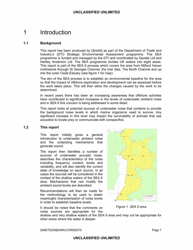
This report has been produced by QinetiQ as part of the Department of Trade and Industry’s (DTI) Strategic Environmental Assessment programme. The SEA programme is funded and managed by the DTI and coordinated by Geotek Ltd and Hartley Anderson Ltd. The SEA programme divides UK waters into eight areas. This report is part of the SEA 6 process which covers the area from Milford Haven northwards through St Georges Channel, the Irish Sea, The North Channel and up into the outer Clyde Estuary (see figure 1 for map).

The aim of the SEA process is to establish an environmental baseline for the area so that the impact of offshore exploration and development can be assessed before the work takes place. This will then allow the changes caused by the work to be determined.

In recent years there has been an increasing awareness that offshore activities have contributed to significant increases in the levels of underwater ambient noise and in SEA 6 this concern is being addressed in some detail.

This report looks at potential sources of underwater noise that combine to provide the background noise levels in which marine organisms need to survive. Any significant increase in this level may impact the survivability of animals that use acoustics to locate prey or communicate with conspecifics.

1.2 This report

This report initially gives a general introduction to underwater ambient noise and the underlying mechanisms that generate sound.

The report then identifies a number of sources of underwater acoustic noise, describes the characteristics of the noise including frequency content, levels and variability, and will also identify the current state of knowledge on each source. In all cases the sources will be considered in the context of the shallow waters of the SEA 6 area. Mechanisms that can modify the ambient sound levels are described.

Recommendations will then be made for the methodology to be used to obtain meaningful characterisation of noise levels in order to establish baseline levels.

It should be noted that the comments on noise sources are appropriate for the shallow and very shallow waters of the SEA 6 area and may not be appropriate for other areas where the water is deeper.

Figure 1. SEA 6 area




2 Underwater ambient noise

2.1 What is ambient noise

Ambient noise is that sound received by an omni-directional sensor which is not from the sensor itself or the manner in which it is mounted. Noise from the sensor or its mounting is termed self-noise. Ambient noise is made up of contributions from many sources, both natural and anthropogenic. These sounds combine to give the continuum of noise against which all acoustic receivers have to detect the signals they are looking for.

Some researchers define ambient noise as the residual when identifiable sources, such as passing shipping, are removed. For this document the definition used is all contributions of noise, both local and distant, since this is the level that impacts bioacoustic receivers.

Ambient noise is generally made up of three constituent types – wideband continuous noise, tonals and impulsive noise. Impulsive noise is transient in nature and is generally of wide bandwidth and short duration. It is best characterised by quoting the peak amplitude and repetition rate. Continuous wideband noise is normally characterised as a spectrum level, which is the level in a 1 Hz bandwidth. This level is usually given as intensity in decibels (dB) relative to a reference level of 1 micro Pascal (µPa). Tonals are very narrowband signals and are usually characterised as amplitude in dB re 1µPa and frequency. Ambient noise covers the whole acoustic spectrum from below 1 Hz, to well over 100 kHz. Above 100 kHz, the ambient noise level drops below thermal noise levels.

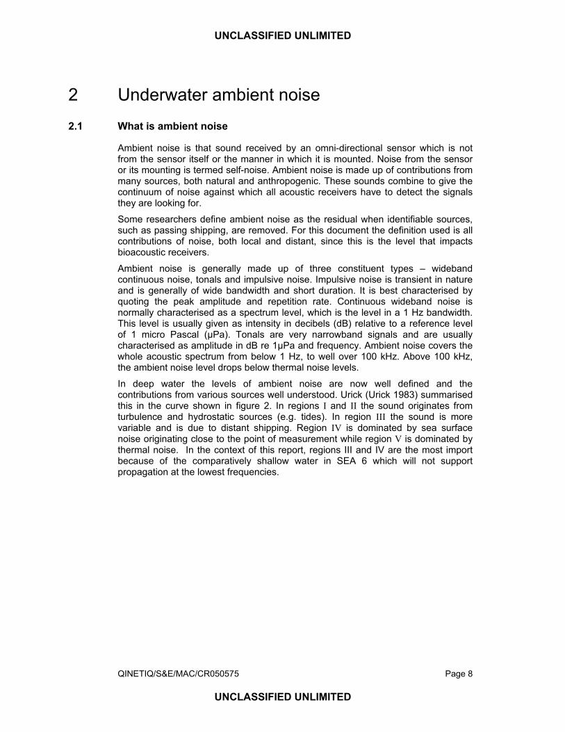
In deep water the levels of ambient noise are now well defined and the contributions from various sources well understood. Urick (Urick 1983) summarised this in the curve shown in figure 2. In regions I and II the sound originates from turbulence and hydrostatic sources (e.g. tides). In region III the sound is more variable and is due to distant shipping. Region IV is dominated by sea surface noise originating close to the point of measurement while region V is dominated by thermal noise. In the context of this report, regions III and IV are the most import because of the comparatively shallow water in SEA 6 which will not support propagation at the lowest frequencies.




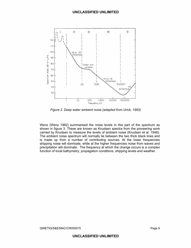
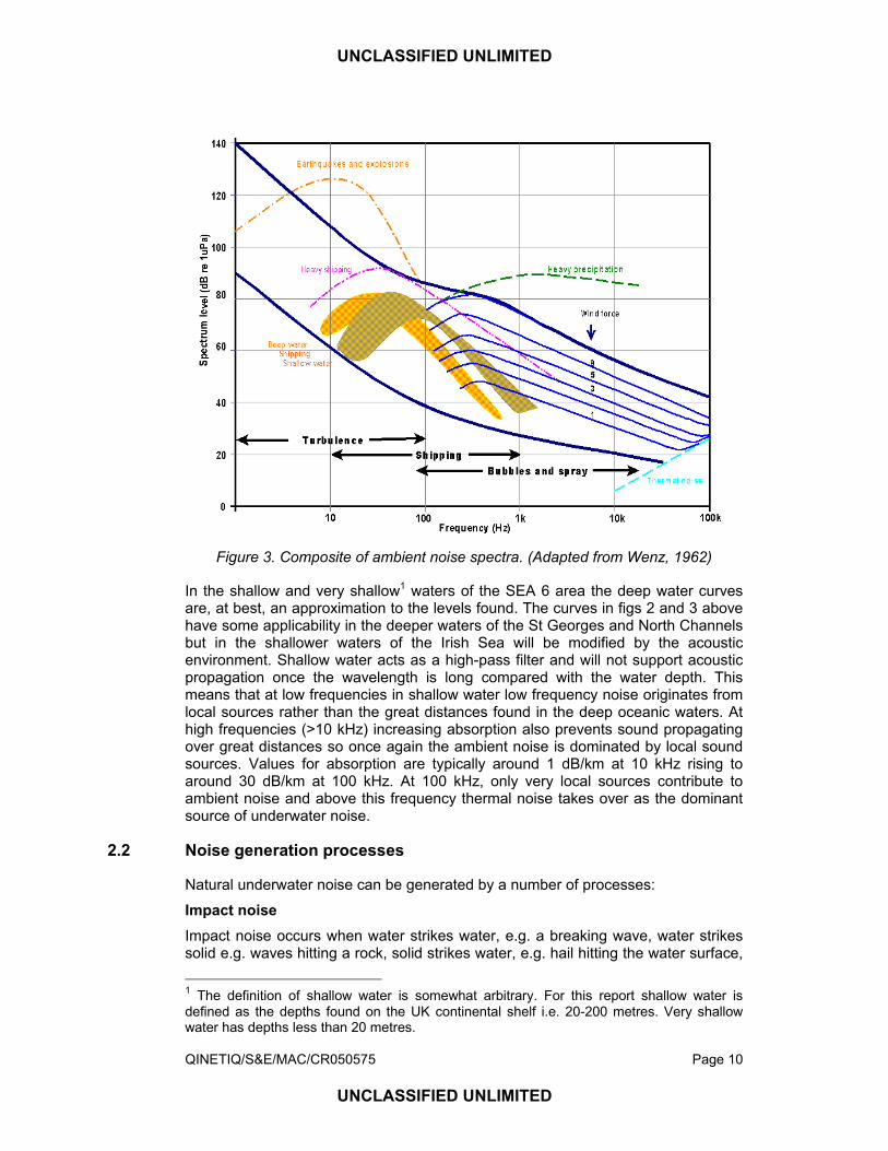
Wenz (Wenz 1962) summarised the noise levels in this part of the spectrum as shown in figure 3. These are known as Knudsen spectra from the pioneering work carried by Knudsen to measure the levels of ambient noise (Knudsen et al. 1948). The ambient noise spectrum will normally lie between the two thick black lines and is made up from a number of contributing sources. At the lower frequencies shipping noise will dominate, while at the higher frequencies noise from waves and precipitation will dominate. The frequency at which the change occurs is a complex function of local bathymetry, propagation conditions, shipping levels and weather.

Figure 2. Deep water ambient noise (adapted from Urick, 1983)




Figure 3. Composite of ambient noise spectra. (Adapted from Wenz, 1962)

In the shallow and very shallow1 waters of the SEA 6 area the deep water curves are, at best, an approximation to the levels found. The curves in figs 2 and 3 above have some applicability in the deeper waters of the St Georges and North Channels but in the shallower waters of the Irish Sea will be modified by the acoustic environment. Shallow water acts as a high-pass filter and will not support acoustic propagation once the wavelength is long compared with the water depth. This means that at low frequencies in shallow water low frequency noise originates from local sources rather than the great distances found in the deep oceanic waters. At high frequencies (>10 kHz) increasing absorption also prevents sound propagating over great distances so once again the ambient noise is dominated by local sound sources. Values for absorption are typically around 1 dB/km at 10 kHz rising to around 30 dB/km at 100 kHz. At 100 kHz, only very local sources contribute to ambient noise and above this frequency thermal noise takes over as the dominant source of underwater noise.

2.2 Noise generation processes

Natural underwater noise can be generated by a number of processes:

Impact noise Impact noise occurs when water strikes water, e.g. a breaking wave, water strikes solid e.g. waves hitting a rock, solid strikes water, e.g. hail hitting the water surface, 1 The definition of shallow water is somewhat arbitrary. For this report shallow water is defined as the depths found on the UK continental shelf i.e. 20-200 metres. Very shallow water has depths less than 20 metres.




or solid strikes solid underwater, e.g. sediment noise. It is usually a broadband, transient noise, possibly with resonant peaks if solids are involved.

Bubble noise There are several types of bubbles in sea water. Passive bubbles are quiescent and do not generate noise. Active bubbles are formed during an energetic process such as breaking waves or rain striking the surface. These bubbles oscillate and generate comparatively narrowband signals centred on the resonant frequency of the bubble.

Turbulence Turbulence associated with surface disturbance or turbulent tidal flow around an obstruction generates low frequency continuous noise.

Seismic Movement of the seabed can be coupled into the water column and generate very low frequency noise.

Anthropogenic noise can be generated by all of the above processes. As an example, a ship moving through the water will generate impact noise by wave slap, bubble noise from entrained bubbles due to the propulsion and passage through the water and turbulence noise due to the disturbed water. In addition a number of additional generation processes may be encountered:

Cavitation Propellers and other fast moving objects in the water can cause cavitation noise when the pressure in the flow around the moving object goes sufficiently negative. This causes cavitation bubbles which very quickly collapse, causing a loud transient sound. The resulting spectrum is wideband but generally has a peak between 100 Hz and 1 kHz.

Machinery noise Machinery generally produces a broadband continuous spectrum with tonals superimposed resulting from the rotation rates of the various parts of the machinery. There may also be impulsive sounds.

Tonals Some systems either deliberately, or as a by-product, generate high levels of tonal signals e.g. Sonar systems, seal scarers.




3 Sources of ambient noise

3.1 Wind-sea noise

A number of early observations of ambient noise suggested that between 500 Hz and 25 kHz the ambient noise levels were dependent on wind speed. Based on these observations the Knudsen spectra were defined relating noise level to wind speed/sea state as shown in figure 3. Later observations showed that that the noise level was dependant on wind speed in the vicinity of the receiver.

The dominant mechanism for the generation of wind-sea noise at the ocean surface is breaking waves, although this mechanism is still not fully understood. Laboratory measurements reported by Medwin et al (Medwin and Beaky 1989; Medwin and Daniel 1990) demonstrated that the characteristic 5dB/octave slope of the Knudsen wind-sea noise spectra results from the incoherent sum of the noise from individual resonant bubbles. At higher sea states, with vigorous breaking waves, large amounts of air are entrained and bubble oscillations may be coupled, leading to collective oscillation of bubbles in a plume (Prosperetti 1988). Melville (Melville et al. 1993) found that the sound radiated by breaking waves increases with sea state and is related to the volume of air entrained as a result of waves breaking.

The dependence on wind speed holds even below the speeds that produce breaking waves and this may be due to noise from flow noise as the wind passes over the sea surface and/or by bubbles induced from turbulence produced at the sea surface by the wind.

An approximate formula for estimating wave noise at wind speeds up to 30 mph and for frequencies in the range 1 to 35 kHz is:

( ) ( )Windspeedwindnoise 10Log*βαdB +=

where α and β are frequency dependant factors

The frequency dependence is caused by the resonance effects in the bubbles trapped below the sea surface and by frequency dependant absorption of noise by this bubble layer. A maximum noise level is reached at wind speeds of 25-30 mph because of increasing absorption of the sound by the bubble layer.

To determine wind-sea related ambient noise levels in a particular area a knowledge of the wind statistics are needed and from this an assessment of the contribution of wind-sea noise can be made. The contribution of wind-sea noise to ambient noise levels is made up of locally generated noise and noise that propagates from a distance by means of multiple surface and bottom reflections. The seabed therefore can have a significant influence on the propagation of wind-sea noise (Buckingham and Jones 1987) and information on seabed acoustic properties is required.

There is likely to be a diurnal and annual cycle in the contribution of wind noise to ambient noise levels due to seasonal and diurnal changes in the meteorological conditions and water column properties.




3.2 Precipitation noise

Precipitation in the form of rain or hail can cause significant elevation of ambient noise levels in the 1 to 100 kHz region. The noise is generated by a number of effects. These are impact noise as the rain/hail impacts the surface of the water, oscillation of the bubble entrained by the raindrop and large raindrops can cause a more complex multiple bubble and multiple impact noise. At low wind speeds bubble oscillation is the dominant noise source in UK waters while impact noise dominates at higher wind speeds.

A good approximate equation for noise from precipitation in the frequency range 1 – 15 kHz is:

( ) ( )RainrateδγRainnoise 10log*dB +=

where Rainrate is in mm/hr

and γ and δ are both frequency and wind speed dependant.

The wind speed dependence is caused by a reduced probability of bubble entrapment and an increase in impact noise as the wind speed increases.

Small rain drops (<1.1mm diameter) produce two sounds as they strike the surface of the sea (Medwin et al. 1990; Medwin et al. 1992). The initial impact produces a short broadband pulse while the oscillating microbubble produced by the impact generates a decaying signal centred near 15 kHz. Noise from rain with small drops in calm conditions has a spectral peak around 15 kHz with a slow fall off above this frequency and a fast drop off below this frequency. Between 2 and 10 kHz there is a flat region (Scrimger et al. 1987). As the wind speed increases the peak at 15 kHz becomes more rounded and fewer bubbles are produced. As the rain drop size increases (1.1 to 2.2 mm diamater) the microbubble is no longer formed and the noise is entirely due to impact noise. For large rain drops (>2.2mm diameter) a different type of bubble is formed and this produces a decaying signal with a centre frequency sweeping from 10 kHz to 30 kHz (Medwin et al. 1992).

Hail produces a broad peak in noise between 2 and 5 kHz, depending on particle size, and this peak frequency has little dependence on wind speed (Scrimger et al. 1987).

Heavy snow falling under calm conditions produces a rising spectra from 20 kHz to over 50 kHz. (Scrimger et al. 1987). It is likely that there is a spectral peak at some frequency above 50 kHz, determined by the snowflake size.

Instruments that measure rainfall rate by measuring the increase in level and spectral shape of ambient noise due to rain drops have recently been developed (e.g. Metocean Data Systems, NS, Canada). These measure the noise levels in a number of channels in the 500 Hz to 50 kHz region.

To estimate the contribution of precipitation noise to ambient noise, knowledge of the statistics of precipitation for the area of interest is needed. It is then possible to integrate the annual cycle to calculate the relative contribution of precipitation to ambient noise levels. There will be an annual cycle in the variation of the contribution of precipitation noise to ambient noise.

3.3 Shore/surf noise Surf noise can make a significant contribution to the ambient noise field in the near-shore region out to at least 9 km offshore (Wilson et al. 1985). The study of ambient




noise in the open ocean and in coastal waters is a well-established field, but few researchers have addressed the nature of the sources and the properties of ambient noise due to surf. Most of the published work on surf noise describes measurements made a few kilometres offshore (Wilson et al. 1985; Wilson et al. 1997), although some measurements have been made in the vicinity of the surf zone (Bass and Hay 1997; Deane 1997; Deane 1999; Deane 2000b; Deane 2000a). Assessment of the nature and scale of the contribution of surf noise to the ambient noise field offshore can be achieved by considering the aspects described in the following paragraphs.

3.3.1 Beach profile and beach face sediment

The beach profile and beach face material must be considered in an assessment of surf noise. The beach profile is required for surf prediction. The beach face material (specifically the grain size of the beach sediment) determines the magnitude and frequency content of noise produced by sediment disturbance in the surf zone. The beach profile depends on factors such as the grain size of the beach sediment, wave steepness, exposure of the beach to wave attack, and the tidal range. In addition almost all beaches are subject to large fluctuations in size and shape. Onshore sediment migration occurs during long-period waves, whilst large amplitude, short period waves cause beach erosion. There is therefore a seasonal cycle of beach profile which is related to the seasonal storm activity.

3.3.2 Noise sources in the surf zone

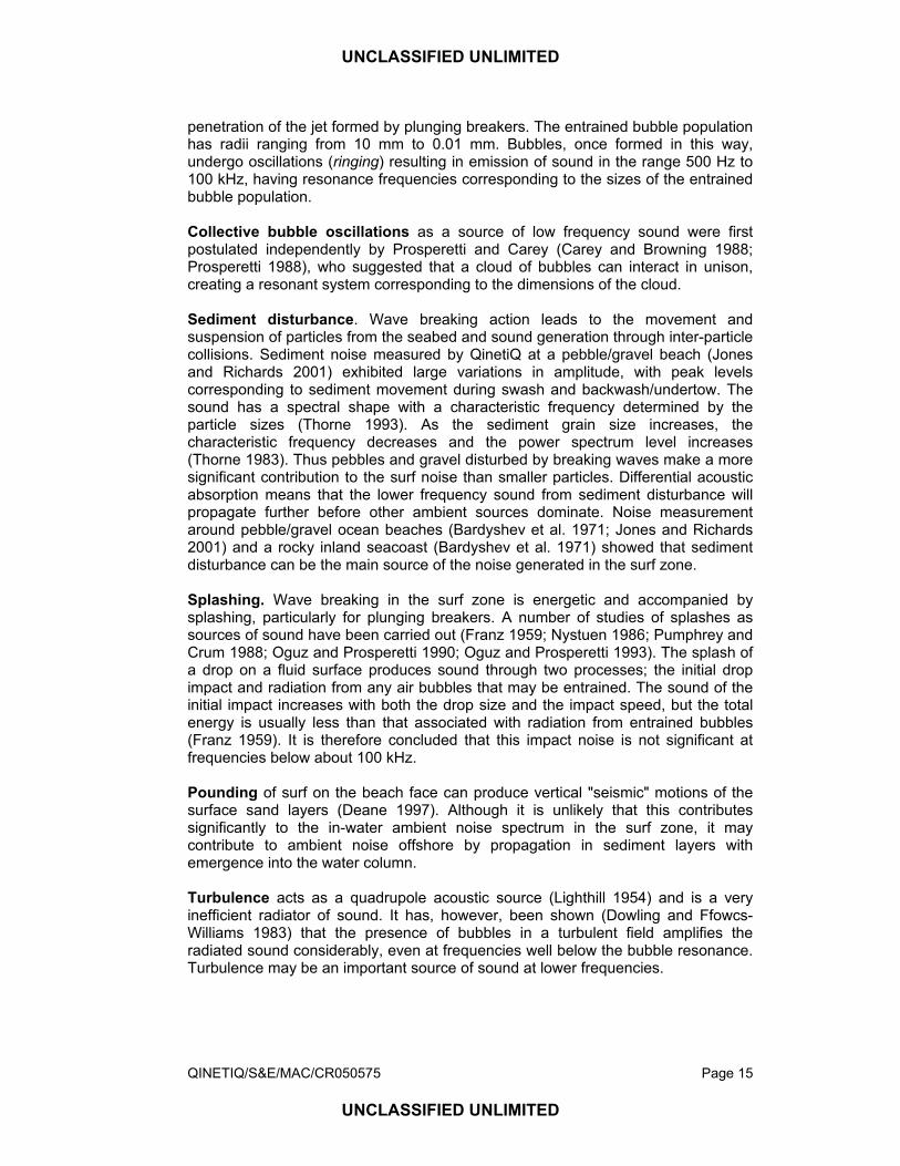
Breaking waves in the surf zone generate sound through a number of different mechanisms. The sound sources are all located in the breaking region and radiate from a few tens of Hz to 500 kHz or more. Figure 4 illustrates the various contributions to the surf noise spectrum. It is not possible to represent the contributions as amplitude spectra, since this depends on local wave and beach conditions.

1 10 100 1000 10000 100000 1000000Frequency (Hz)

Turbulence and surfseisms

Collective bubble oscillations Free bubble oscillations Splashing

Sediment noise - Saltation

Pebbles Sand

Figure 4. Contributions to surf noise spectrum

Free bubble oscillations. Large quantities of air are entrained into the water as a result of breaking waves in the surf zone. According to Melville (Melville 1996), after initial entrainment a volume of air is broken up into smaller and smaller bubbles. In addition, bubbles are formed by drops that impact on the water surface and by the




penetration of the jet formed by plunging breakers. The entrained bubble population has radii ranging from 10 mm to 0.01 mm. Bubbles, once formed in this way, undergo oscillations (ringing) resulting in emission of sound in the range 500 Hz to 100 kHz, having resonance frequencies corresponding to the sizes of the entrained bubble population. Collective bubble oscillations as a source of low frequency sound were first postulated independently by Prosperetti and Carey (Carey and Browning 1988; Prosperetti 1988), who suggested that a cloud of bubbles can interact in unison, creating a resonant system corresponding to the dimensions of the cloud. Sediment disturbance. Wave breaking action leads to the movement and suspension of particles from the seabed and sound generation through inter-particle collisions. Sediment noise measured by QinetiQ at a pebble/gravel beach (Jones and Richards 2001) exhibited large variations in amplitude, with peak levels corresponding to sediment movement during swash and backwash/undertow. The sound has a spectral shape with a characteristic frequency determined by the particle sizes (Thorne 1993). As the sediment grain size increases, the characteristic frequency decreases and the power spectrum level increases (Thorne 1983). Thus pebbles and gravel disturbed by breaking waves make a more significant contribution to the surf noise than smaller particles. Differential acoustic absorption means that the lower frequency sound from sediment disturbance will propagate further before other ambient sources dominate. Noise measurement around pebble/gravel ocean beaches (Bardyshev et al. 1971; Jones and Richards 2001) and a rocky inland seacoast (Bardyshev et al. 1971) showed that sediment disturbance can be the main source of the noise generated in the surf zone. Splashing. Wave breaking in the surf zone is energetic and accompanied by splashing, particularly for plunging breakers. A number of studies of splashes as sources of sound have been carried out (Franz 1959; Nystuen 1986; Pumphrey and Crum 1988; Oguz and Prosperetti 1990; Oguz and Prosperetti 1993). The splash of a drop on a fluid surface produces sound through two processes; the initial drop impact and radiation from any air bubbles that may be entrained. The sound of the initial impact increases with both the drop size and the impact speed, but the total energy is usually less than that associated with radiation from entrained bubbles (Franz 1959). It is therefore concluded that this impact noise is not significant at frequencies below about 100 kHz. Pounding of surf on the beach face can produce vertical "seismic" motions of the surface sand layers (Deane 1997). Although it is unlikely that this contributes significantly to the in-water ambient noise spectrum in the surf zone, it may contribute to ambient noise offshore by propagation in sediment layers with emergence into the water column. Turbulence acts as a quadrupole acoustic source (Lighthill 1954) and is a very inefficient radiator of sound. It has, however, been shown (Dowling and Ffowcs-Williams 1983) that the presence of bubbles in a turbulent field amplifies the radiated sound considerably, even at frequencies well below the bubble resonance. Turbulence may be an important source of sound at lower frequencies.




3.3.3 Sound propagation from the surf zone

Sound propagation out of the surf zone is initially through the dynamic inshore region, which presents a difficult analytical problem compared with open water propagation prediction. The main environmental features that affect acoustic propagation in the inshore region are the slope of the beach and seabed and the high concentrations of bubbles. Bubbles in the surf zone will influence propagation towards deeper water, as both individual bubbles and bubble plumes will strongly absorb and scatter the sound. In patches of high bubble concentration, the sound speed can be reduced to 500 ms-1 and acoustic absorption can be as high as 50 dBm-1 (Deane 2000b). Similarly the presence of sediment particles, suspended in the water column by wave and current action, have been shown to absorb and scatter sound, particularly at high frequencies (Richards et al. 1996). There are no models currently available that will represent the complexities of propagation in the surf zone and inshore region. An empirical approach is recommended, based on measurements published in the open literature. A wave refraction model for wave propagation inshore (WAVECALC) and a surf prediction tool (SURFtool) have been developed by QinetiQ (Li 1998a; Li 1998b; Jones 1999) and have been proposed as the first stages of a coupled ocean-acoustic modelling system for the prediction of surf noise (Jones et al. 2000; Jones and Richards 2001). WAVECALC requires information on incident swell conditions offshore, which may be forecast or obtained from a climatological database, and provides parameters required by SURFtool (i.e. significant wave height, period and direction). SURFtool predicts breaker type, height, period and number of lines of surf, which may be used to assess the spectral characteristics and temporal variations of noise sources in the surf zone. WAVECALC and SURFtool require detailed information on the bathymetry of the inshore region and beach profile respectively. Further offshore, the acoustic modelling may be undertaken using widely available wave-theory or ray-theory numerical simulations. It is possible to make some general comments on the nature of surf noise in the SEA 6 area. In coastal waters near sandy beaches e.g. Morecambe Bay, surf noise will be dominated by resonant bubble noise. Single bubble oscillations contribute to the radiated noise spectrum of surf noise from 500 Hz to 100 kHz. The higher frequencies (above 10 kHz) will be subject to acoustic absorption that increases with frequency. Collective bubble oscillations will generate sound below about 100 Hz, but this is unlikely to propagate in the water column, being below the cut-off frequency in the very shallow waters characteristic of slowly-shelving sandy beaches. On sandy beaches it is unlikely that sediment disturbance will contribute much below about 100 kHz. It should also be noted that the very shallow shelving angle means that there may not be a distinct surf zone. At the coast near cobble, pebble or coarse gravel beaches e.g. West Wales coast, surf noise will be dominated by sediment disturbance. The characteristic frequency and level of the sound depends on the sediment grain size – as the size increases, the frequency decreases and its level increases. Cobbles, pebbles and coarse gravel therefore make a more significant contribution to surf noise than fine gravel or sand. Sediment disturbance contributes to the radiated noise spectrum of surf noise from below 200 Hz with a peak at 1 to 2 kHz and a steep roll-off above 5 kHz. Bubble noise will also be present at higher frequencies. Beaches where sediment




disturbance is important are steeper than sandy beaches, but surf noise will nevertheless be subject to a low-frequency cut-off that varies on a timescale corresponding to that of the breaking wave period (Jones and Richards 2001). Little work has been carried out to measure noise from rocky shorelines, particularly the ultimate example of a vertical cliff. It is likely that there will be contributions from impact noise and from the impact of spray thrown back from the rock face. In summary, surf noise from sandy beaches will contribute to the offshore ambient noise spectrum at frequencies over the range 500 Hz to 10 kHz. Noise from steeper, cobble, pebble or gravel beaches will contribute over the range 200 Hz to 5 kHz. Surf noise may be detected and will contribute to the ambient noise spectrum to at least 9 km offshore. Rocky foreshores will have contributions from turbulence, bubble oscillation and impact, but there will be no sediment noise so noise levels will generally be lower in the 1-50 kHz region compared with sand or gravel shores.

3.4 Sediment transport noise

Under some circumstances it is possible for the sediment on the seabed surface to become highly mobile. The surf zone, described above, is perhaps the obvious example, but sediment transport can also occur away from the shoreline. Sediment transport occurs when the water is shallow (<10 metres), there is a current running and there is significant wave height to disturb the seabed. This occurs mostly with light sediments such as clays or fine sand. The sediment collides with itself and obstacles on the seabed and this generates high frequency noise. The noise is mostly above 10 kHz with peak frequencies at a few tens of kHz. The actual spectrum will depend on particle size and material. The effect has been observed in the English Channel (Pers Obs2), (Thorne 1985), the North Sea (Voglis and Cook 1970), and the Bristol Channel (Pers Obs3). The effect can last for periods of less than a minute up to periods greater than an hour, depending on the tidal conditions.

Measuring sediment transport noise is very difficult. Deploying a hydrophone can result in noise levels elevated up to 40 dB above ambient during major events, but most of this noise is caused by the particles hitting the hydrophone and its surrounds and it is then questionable whether one is measuring ambient noise or self noise. In terms of impact on a biological receptor, the impact noise is likely to be less because of the nature of flesh compared with metalwork or hard epoxy encapsulant. It is also likely that the receptor would choose to move out of the main sediment flow for a number of reasons. However, in some parts of the SEA 6 area, particularly the shallow sandy areas in the eastern Irish Sea, sediment transport is a common effect and the resulting noise should be characterised in order to fully understand the ambient noise levels in the area.

The noise contribution to ambient noise will vary with the tidal cycle, the lunar cycle and the annual cycle.

2 A hydrophone 1.5 metres above the mixed sand and broken shell seabed in Durlston Bay detected noise levels raised by 40 dB at 15-20 kHz during easterly gales and mid-tide. 3 A hydrophone deployed mid-water in the tidal rip off Bull Point detected noise levels raised by ~20 dB at 15-20 kHz for 30 minutes during the flood tide.




3.5 Aggregate extraction

The dredging of deep deposits of gravel is inherently a noisy operation. The resulting noise is a mixture of mechanical noise from operation of the dredge and a noise similar to sediment transport noise resulting from the disturbance of the gravel. Two areas are known to be licensed (Jones et al. 2004), One is 30 km offshore from Barrow in Furness, the other 25 km off Liverpool. A third, also off Liverpool has a licence pending.

No published information on noise levels from aggregate extraction in the SEA 6 area has been identified in the course of this study. There is some published information on aggregate extraction in the English Channel (CEFAS 2003) and dredging activity associated with oil field development (Greene 1987) but this is likely to have been carried out in different water depths, over different sediment types and with different types of dredgers. It is believed that a number of other acoustic measurements have been made of aggregate extraction activity but the information is in company reports and could not be obtained during this short study.

3.6 Commercial shipping

The SEA 6 area carries a considerable amount of shipping. This mostly originates from traffic to and from the major ports of Liverpool, Dublin and Belfast together with traffic moving north and south through the Irish Sea. The other major contributor to shipping movements is the ferry traffic between Britain and Ireland. Other shipping routes link the smaller ports to the main shipping lanes.

Shipping noise is the dominant contribution to ambient noise in shallow water areas close to shipping lanes and in deeper waters. Shipping noise is most evident in the 50-300 Hz frequency range. At longer ranges the sounds of individual ships merge into a background continuum. At higher frequencies the dominant noise source is likely to be locally-generated wind noise. Shallow water acts as a high pass filter, with the cut-off frequency increasing as the water get shallower. In very shallow coastal waters distant shipping noise makes little or no contribution to ambient noise. See section 6 for a discussion on shipping sound field modelling.

Close to ships under way the noise spectrum splits into a number of regions. At low frequencies below 1 kHz there is a continuous wideband spectrum of noise with a number of tonals originating from rotating machinery superimposed. Above 1 Khz the machinery noise diminishes and water displacement noise becomes dominant This drops below other sources of noise above 20 kHz. Additional noise may be caused by propeller cavitation and faulty machinery. Strong tonals can be generated by a singing propeller4, a faulty gearbox or by electrical generation machinery. As an example a recent set of measurements for an 11 metre workboat revealed a tonal on 800 Hz that was 40 dB stronger than the other noise sources on the boat. This was traced to a faulty gearbox (Wharam et al. 2004).

Different types of ships have different contributions from the different noise sources. For a fast ferry, the major noise sources are from displaced water in the 5-20 kHz

4 Propellers can oscillate strongly when the resonant blade is excited by vortex shedding from the blade tips. The tonal is usually in the 100-1000 Hz region. See Anon (2003) Singing propellers. Hydrocomp Inc, Report 138, Durham, NH, USA (www.hydrocompinc.com/knowledge/library.htm) for a more detailed explanation of the effect.




region plus strong tonals on a few hundred Hz from the machinery, while for a small coaster virtually all of the noise is from the propulsion machinery below 200 Hz.

Away from the main shipping lanes a major contribution is likely to come from fishing boats, particularly in the fishing grounds around the Isle of Man and the southern St Georges Channel. There is also likely to be fishing traffic around all of the smaller ports with fish landing facilities.

Shipping noise will vary on a diurnal cycle (ferry and coastal traffic) and an annual cycle (seasonal activity).

3.7 Leisure craft

Over a number of years there has been a steady increase in the numbers and types of leisure craft in use around the UK. There has also been a steady increase in the engine power available to such craft. This has resulted in a considerable increase in underwater noise levels produced by this class of sound source and in holiday areas this can be the dominant sound source through the summer months. A number of workers have attempted to gather statistics on leisure craft traffic, particularly with regard to environmental impact (Gibbons 2000; Haviland et al. 2001).

Leisure craft can generally be grouped into a number of classes:- • Sail powered craft • Slow motorboats • High-speed motorboats • Personal watercraft

Sail powered craft are generally very quiet with the only sound coming from flow noise, wave slap and rigging noise. Racing yachts produce higher noise levels because of their increased speed, but are still much quieter than motorboats travelling at the same speed. Slow motorboats generally produce low frequency noise from propulsion machinery containing broadband and tonal components, plus higher frequency broadband noise due to water impact and disturbance. High-speed motorboats use one or more high-powered engines to achieve planing speeds and generally cause considerable disturbance to the water surface. As well as the low frequency sounds, often with loud tonal components from the machinery, the high frequency sounds are enhanced by the disturbed water thrown up by the passage of the boat through the water impacting the surface of the water and generating broadband noise. This noise typically dominates the signature in the region 5-25 kHz. Personal watercraft, such as jet skis, are generally very small craft capable of carrying just one person, but fitted with a high power engine. The propeller is normally ducted and this reduces the noise output. The engines and impellers usually operate at high speeds so the predominant noise output is higher in frequency than other leisure craft. Leisure craft activity is highest around their home ports where they are used for day running. Other common activities include racing and port to port cruising. Because they generally use the smaller ports or purpose built marinas the main leisure craft routes are generally separated from the commercial shipping routes and are usually closer inshore.




Variations in leisure craft noise occur on a number of cycles. The diurnal cycle is generally bimodal with a morning peak as craft leave harbour and move out to whatever activity they are undertaking plus a second peak late afternoon as the craft return to harbour. These two peaks are superimposed on a broader day/night cycle with much reduced activity through the night. On a weekly basis there is a broad peak in noise corresponding to weekend activity. There is also an annual cycle with much increased activity through the summer months and very little activity through the winter months.

There is generally a good understanding of the noise levels produced by the different vessel classes but there appears to be little information on the numbers and distribution of such craft through the year. It is also not clear how the very different noise contributions from the different types of craft combine to contribute to the ambient noise levels and spectra.

3.8 Industrial noise – offshore

Offshore industrial noise includes the noise generated by the operation of offshore wind farms, oil and gas rigs and offshore construction noise.

Oil and Gas rigs generate noise by conduction of the noise from machinery on the platform into the water column. This is likely to comprise low frequency tonal noise from the rotating machinery (<1 kHz) and a wideband noise level made up of many individual contributions from all the noises sources on a typical rig. A literature search of peer-reviewed journals did not find any information on the noise fields around oil and gas rigs.

Wind farm operational noise is likely to originate from machinery noise coupling via the tower into the water column and/or substrate and also from the rotating blades coupling via air movement into the water surface. A likely third source will be noise from the power cables to the shore. When cables carry high alternating currents the magnetic field around each core causes alternate attraction and repulsion and this can result in physical movement and hence a signal in the water. As well as the cables to operational wind farms there are a number of power cables across the Irish Sea carrying power between the mainland and the Isle of Man and between Britain and Ireland. Again, a literature search failed to find any papers on the noise from wind farms in the peer-reviewed journals and only a very small number in the grey literature. (Koschinski et al. 2003; Danneskiold-Samsoe 2005).

The construction of offshore and near-shore facilities such as wind farms or harbours may involve pile driving and this is inherently a noisy operation. Nedwell recorded source levels as high as 262 dB re 1uPa@1m for piling associated with the construction of the North Hoyle and Scroby Sands wind farms (Nedwell et al. 2004). Sounds from harbour construction pile driving have been heard 50 miles away

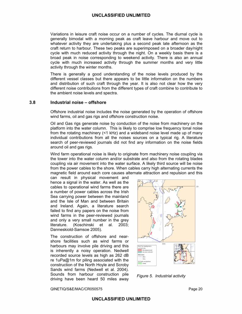
Figure 5. Industrial activity




(Pers Obs5). Attempts have been made to reduce the radiated noise by using bubble curtains around piling sites (Wursig et al. 2000) with limited success.

Within the SEA 6 area the main offshore activity is along the North Wales coast, past Liverpool and then northwards into the Morecambe Bay oil and gas production area. It is believed there may be some wind farm activity along the Irish coast north of Dublin. Noise from the oil and gas fields and wind farms will only show a weak dependence on the tidal cycle while wind farm noise will also be dependant on the annual cycle of wind strength variations. Figure 5 shows the location of present and planned oil and gas fields and wind farms in the SEA 6 area.

3.9 Industrial noise – onshore

Industrial activity onshore adjacent to the coastline can produce underwater noise by coupling through the substrate. Noise levels are only significant if the noise is intense e.g. quarry blasting6, or if there are a number of noise sources e.g. an area of heavy industry.

Transport systems close to the coastline e.g. motorways or railway lines can also couple noise into the underwater environment via the substrate.

The coupling through the substrate will generally only occur at very low frequencies (<100 Hz).

A literature search found no information on levels or spectra from this type of source.

3.10 Military noise

The military can generate underwater noise by the use of ships, aircraft, explosives and/or active sonar transmissions. Active sonar use within the SEA 6 area is confined to military exercises, see the next section for more details on sonar.

Military ships are generally very quiet and make only a small contribution to overall shipping noise. The sounds generated by explosives are very impulsive close to the event, but long-distance propagation smears the energy in time and frequency to give sounds above ambient for many seconds. There are a number of areas where military exercises may take place:

Lower Clyde exercise areas

Port Patrick range

Aberporth test range

All of these are believed to have a very low usage of explosives and although the event may have a major impact in the vicinity of the activity, the total contribution to ambient noise levels will be very low.

5 During a cruise in the Tyrrhenian Sea, pile driving in Monaco harbour was clearly heard on a hydrophone deployed off the north coast of Sardinia. 6 Quarry blasting in the Purbecks, Dorset, can be clearly heard on a hydrophone 400 metres offshore and 3 miles from the quarry.




3.11 Sonar

Sonar is widely used by leisure, fishing and commercial vessels and there is also some limited military usage within the SEA 6 area. Typical sonars currently in use are:

• Echosounders

• Fish-finding sonars

• Fishing net control sonars

• Acoustic modems

• Air guns for seismic surveys and reservoir monitoring

• Military sonar

By far the most prevalent of these is the ubiquitous echosounder. Most vessels from small leisure craft up to the largest commercial ships have at least one echosounder. These work on frequencies from 26 Khz to 300 kHz with source levels up to 220 dB re 1µPa@1m. These sonars direct their energy downwards into the seabed but there is significant energy travelling horizontally either from the sidelobes of the transducer or by scatter off the seabed. The higher frequencies are attenuated quickly by absorption, but the contribution to ambient noise is significant due to the high numbers of such units.

Commercial fishing sonars can also make a major contribution to ambient noise because of the lower frequencies, higher power and greater power directed horizontally . The contribution is mostly limited to the grounds favoured for fishing.

Acoustic modems are used to carry data from seabed installations to the surface and typically work in the range 2-20 kHz, depending on data rate and range required. They are generally omnidirectional and can generate high power levels. It is not known how many are in use in the SEA 6 area but it is likely that they will be in use around the oil and gas fields and also in use by scientific equipment deployed elsewhere in the area.

Air guns are used to generate very high level impulses of low frequency sound directed downwards into the seabed for geological survey work. Source levels may be as high as 250 dB re 1µPa@1m with a centre frequency between 50 and 100 Hz. It is believed that while they were regularly observed 10-15 years ago in the St Georges Channel, their use in the SEA 6 area and adjacent areas is now at a low level. Because of the low frequencies and very high powers in use they can be heard over large areas and, with a high repetition rate, they can make a very significant addition to ambient noise levels over a wide area.

Military sonars use high power transmitters to generate tonal signals in the range 1-10 kHz and with pulse lengths between 0.1 and 4 seconds, depending on mode of operation. When operating they can be heard up to 10 miles away, depending on the propagation conditions, even in the shallow waters typical of the SEA 6 area. The only part of the SEA 6 area where military sonar usage is likely to be significant is in the far north of the area where the lower Clyde exercise areas are occasionally used by frigates and submarines.

No published information has been identified by this study on the statistics of sonar usage. It is not clear how many civilian and military sonars are operating in the SEA 6 area at any one time so it is not possible to accurately judge the contribution to ambient noise levels.




3.12 Aircraft noise

Aircraft noise can couple through the sea surface when an aircraft flies low over the sea surface(Urick 1972). This can happen when fixed wing aircraft approach a runway located on the coast, or a helicopter operates low over the sea. No airports located directly on the coast have been identified within the SEA 6 area, but helicopters are likely to operate within the gas fields and will also be used to service all of the offshore and near-shore lighthouses within the area.

Helicopter noise originates from the disturbance of the sea surface by the down wash from the blades and by coupling of blade noise directly into the sea. The down wash noise is very similar to wind noise in frequency characteristics and is greatest in the 2-20 kHz region. Blade noise contains a number of components originating from the rotation of the blades and the machinery that drives the blades. There are a number of strong tonals in the 10-100 Hz region associated with rotor operation and a strong tonal component at the turbine blade rate which is typically around 10 kHz7.

Within the SEA 6 area, the only area likely to be affected by helicopter noise is around the gas rigs and even here other noise sources are likely to predominate. Noise caused by servicing lighthouses, while it is significant during the event, the events happen so infrequently that there is unlikely to be any major impact on the environment.

Desharnais (Desharnais and Chapman 2002) showed that sonic booms from aircraft can also penetrate into the water column, producing a low frequency pressure pulse. The only current source of such booms in the SEA 6 area is likely to be military aircraft and such booms happen so infrequently that their contribution to ambient noise levels is negligible.

3.13 Fishing activity

Commercial fishing can make a contribution to ambient noise in a number of ways. Apart from the contribution by the vessel noise and the use of sonar to find fish and monitor nets, the most significant contribution is trawl noise, particularly from bottom trawls. The sound of chains and rollers being dragged across the seabed can often be heard several miles from the activity.

The overall noise field from the fishing gear consists of low frequency noise from the rollers, mid and high frequency noise from the general disturbance of the seabed and high frequency noise from the chains. In the very shallow waters of the eastern Irish Sea there is also the possibility that trawling could trigger sediment transport and hence increase the noise levels produced. No published information on absolute levels or typical spectra has been found.

No appropriate statistics on fishing activity were available during the preparation of this report to judge the level of the impact of this noise source. Figure 5.7.2 in the environmental assessment of Irish waters (Anon 1999) suggests that the majority of trawling occurs in the shallow coastal waters northwards from Liverpool to the Solway Firth and in the western Irish Sea in the area northwards from Dundalk to the entrance to Belfast Lough. There is also a less used area extending westwards

7 Most information on helicopter noise is classified by the military. This information was derived from an opportunistic measurement of the Portland search & rescue Sea King helicopter.




from Fishguard in south-west Wales. The Irish Sea Pilot Study (Vincent et al. 2004) carried out by JNCC agrees that the predominant trawling area is to the west and east of the Isle of Man but suggests that the southern area is further south and outside the SEA 6 area. It also adds another high activity area to the south and east of Arran in the Clyde estuary.

Fishing noise is likely to vary on a diurnal cycle, a lunar cycle and an annual cycle.

3.14 Biological noise

Living organisms can make a major contribution to ambient noise levels. Deploying a hydrophone in very shallow waters around the southern and western UK coast will result in a loud random clicking sound being observed. The rate of clicking varies during the course of a day and on an annual basis. It has not been able to identify the organism causing the noise but current ‘best guess’ is the crustacean Alpheus glaber, one of the snapping shrimps. MARLIN (Rowley 2004) records this species as being found in the western English Channel and northwards to the North Channel while Smalldon (Smalldon et al. 1993) also agrees that this species occurs along the southern and western coasts of the UK, but also suggests it is only found in waters more than 30 metres deep. In recent years a small number have been caught in the very shallow waters of Weymouth Bay which suggests they may come into much shallower waters than previously thought. The observed clicks have energy content from around 1 kHz to over 100 kHz, with a peak around 7 kHz, and can occur at rates up to 2-3/sec. Source levels have been estimated to over 200 dB re 1µPa@1m (Pers. obs.8). The sound sources tend to be clumped, with a lower density of clicks between the hot spots.

Many fish can produce sound, particularly as part of the mating process. Although the UK does not have the highly vocal species to be found in tropical seas, many UK fish species can produce some sound.

The most vocal of marine species are the cetaceans and species to be found in the SEA 6 area can produce sounds over the range 2-200 kHz. With numbers low across the whole SEA 6 area due to a number of factors, these sounds only make a significant contribution to ambient noise levels in the southern part of the SEA 6 area and, to a lesser extent, the far north-west of the area.

Cetacean sounds are either tonal whistles in the range 2-25 kHz, or wideband echolocation clicks with maximum energy in the 40-140 kHz region. Source levels for the tonals sounds are around 170-180 dB re 1µPa@1m while echolocation clicks range from a source level of 170 dB re 1µPa@1m for the harbour porpoise (Phocoena phocoena) up to 226 dB re 1µPa@1m for the bottlenose dolphin (Tursiops truncatus).

Biological noise has been observed to vary on a diurnal cycle, a tidal cycle and an annual cycle.

3.15 Thermal noise

In the absence of all other sources of ambient and self noise, the underlying noise level is determined by thermal agitation of the molecules. This noise rises 8 This sound has been observed in hydrophones deployed along the Dorset coast and is most prevalent where there are fixed structures on the seabed, such as reefs or wrecks. It is much less prevalent over mobile sea beds such as sand or mud. Similar sounds have been heard from Gibraltar northwards along the European coastline to the Clyde Estuary.




proportionally with frequency and for real systems is only important above 100 kHz. Ambient noise generally falls with increasing frequency until thermal noise dominates when the slope changes to a 6 dB/octave rise with increasing frequency. The noise spectrum level from thermal noise is given by:

( )FrequencyNt 10hermal Log*2015 +=

Where Frequency is in kHz.




4 Ambient noise field modifiers

4.1 Introduction

Section 3 set out the variety of sources of ambient noise in the SEA 6 area. The sound field at any one site is a composite of many of these sources. In addition to the complicated sum of components there are additional effects which will modify the level and spectral content of the ambient sound field. This section will describe these effects and the sound field modification that may be observed.

4.2 Acoustic propagation

Sound produced by the various ambient noise sources propagates to a receiver through the very complex underwater environment. Because of variation in temperature, salinity and pressure the path followed by the sound waves can deviate markedly from a straight line. The structuring is most marked in the vertical plane, causing sound to be refracted upwards or downwards, depending on the temperature gradient, but horizontal structuring can also be encountered. As sound is refracted up or down it may interact with the surface and the sea bed by reflection and scattering. The level of signal arriving at a distant point is a complex sum of many paths that may or may not interact with the seabed and sea surface.

Variations of salinity are generally very small, except perhaps at the mouth of major rivers, and pressure variations are due entirely to depth so temperature variations have the major effect on sound propagation in shallow water.

Under some conditions, a mixed isothermal layer forms close to the sea surface that traps the acoustic signals and a source and receiver located within this surface duct experience significantly less propagation loss than when there is no surface duct. During the day the sea surface can heat up and introduce a temperature gradient close to the sea surface that causes downwards refraction and hence increased propagation loss.

Because the sound can interact strongly with the seabed, the sediment types and sea bed roughness can affect propagation loss. Similarly, waves on the surface can also affect propagation loss by scattering the sound interacting with the surface rather than just reflecting it.

Suspended sediments or bubbles can also cause additional propagation loss.

Propagation loss varies on a diurnal basis, particularly during the early summer, and on an annual cycle, as the air temperature variations through the year warm and cool the water. A period of sustained strong wind can also disrupt the temperature structuring.

4.3 Multi-path effects

Because of the surface and sea bed reflections sound can travel between a source and receiver by a multitude of paths. This has the effect of dispersing the arrived signal in time. This effect is particularly import for wideband impulsive sounds such as explosions, pile driving or seismic exploration air-guns. If any of the propagation effects are frequency sensitive then frequency dispersion will also occur. A common example of this is the sound of air guns operating at distances of 20-30 miles in




which the low frequencies travel more slowly than the high frequencies so the single impulse at the source turns into a pronounced frequency sweep at the receiver. The effect of time dispersion is to reduce the peak energy in the received signal. The integrated level is unchanged by time dispersion, but the peak levels can be significantly reduced. When considering the contribution to ambient noise levels this can be an important factor.

4.4 Source and receiver depth

The vertical temperature and pressure structure described above can lead to significant variations in the propagation loss between a sound source and the receiver as the depth of the source and/or the receiver is varied. The most extreme example is the surface duct where a shadow zone may form under the duct. Within the shadow zone levels from a distant sound source in the duct are much reduced compared with the level from the same source within the duct.

4.5 Tides

In the very shallow waters to be found in large parts of the SEA 6 area, the variations in depth due to tides cause a significant variation in the depth of water. This can make a significant difference to the ambient noise field in these areas due to changes in the propagation path. Areas of sand banks are particularly affected where low propagation loss paths at high tide can have much higher propagation loss at low tides, particularly at the lower frequencies.

Sand banks that dry at low water can also break acoustic paths so a receiver hearing a loud noise source across a sand bank at high tide may not receive it at low tide.




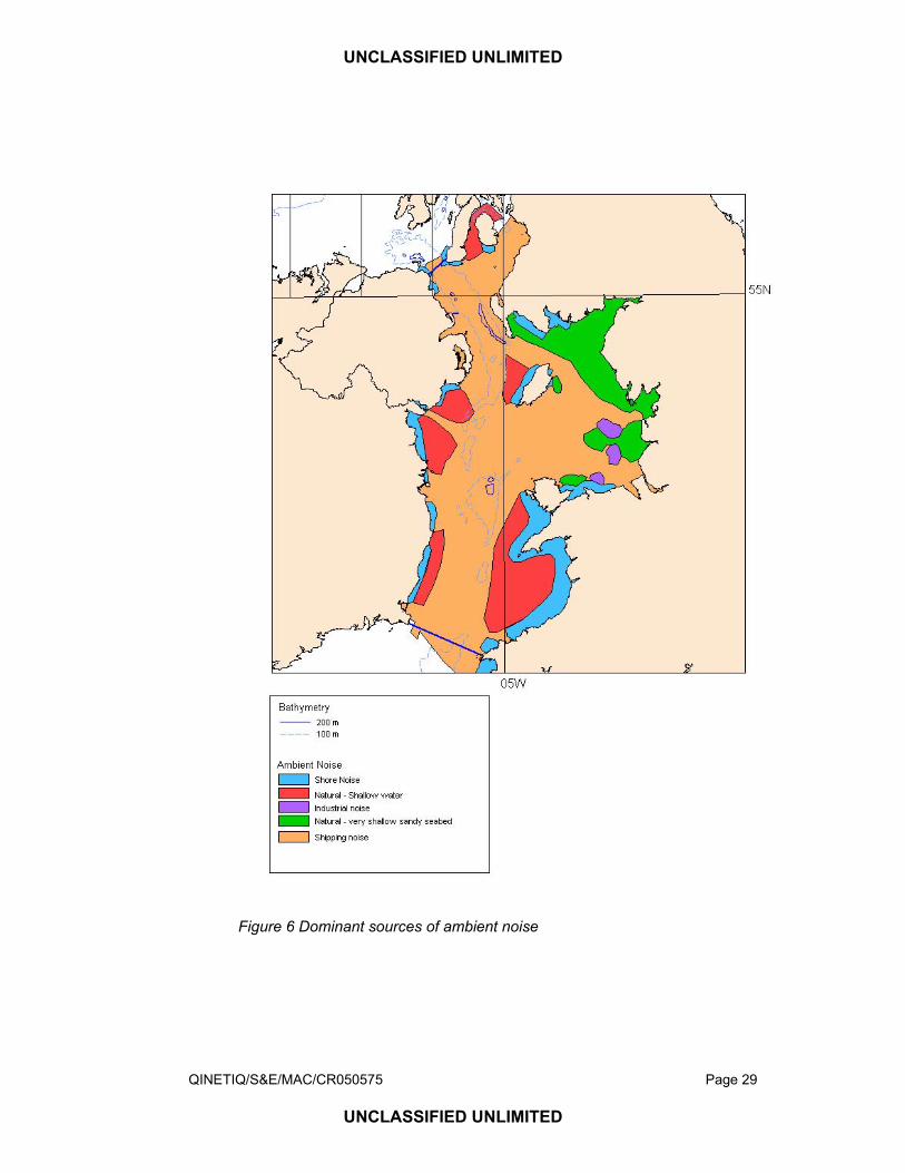
5 Dominant noise sources Section 3 listed the possible contributors to ambient noise within the SEA 6 area while section 4 showed how this sound can be modified by a number of environmental factors. In this section the most likely dominant noise sources across the area are mapped. This information is based on the information gleaned during this study, from the experience of the authors when working in the SEA 6 area and from a much wider experience of studying the various sources of ambient noise over many years of sonar trials.

Figure 6 is a map of the SEA 6 area showing what, in the opinion of the authors, will be the dominant noise sources across the area. Note that this map represents the situation at low wind speeds and no precipitation noise. When the weather deteriorates it is likely that wind and rain noise will dominate over large areas and that surf noise will dominate further offshore. It should also be noted, as shown in section 6 below, that the areas affected by different noise contributions will vary through the year as acoustic propagation loss varies through the seasons.

From figure 6, it can be seen that shipping noise is likely to dominate across large parts of the SEA 6 area. The shoreline is likely to be dominated by surf noise in those areas where there is a shoreline. For large areas of the eastern Irish Sea the angle of shelving is so shallow that, except at extreme low and high tide, there is no distinguishable shore line, so in these areas wind/precipitation/sediment transport noise will dominate. The area offshore of Liverpool is likely to be dominated by industrial noise from the oil and gas production facilities and wind farms.




Figure 6 Dominant sources of ambient noise




6 Characterising sites for ambient noise levels

6.1 Current techniques

When considering the location and impact of offshore developments, knowledge of the baseline ambient noise levels are required in order to be able to judge the likely impact of underwater noise resulting from construction work, the operational phase and decommissioning. The problem is defining what measurements are needed in order to characterise ambient noise levels over a wide geographic area such as the SEA 6 area, which encompasses many types of acoustic environment. The problem is compounded by the variations in ambient noise spectral content and levels on timescales varying from seconds to many years.

Early work used long time-constant averaging, typically with averaging periods measured in minutes. The majority of this early work was in deep water where there is much lower variability compared with shallow water noise levels and this work led to the reference curves shown in section 2.

More recently there has been renewed interest in characterising shallow water ambient noise and this has resulted in a number of specialised measuring systems that look not just at ambient noise spectra and levels, but also assess the anisotropy of the noise. Typical of these systems are the Ambient Noise Sonar (ANS) produced by the Florida Atlantic University (Glegg and Olivieri 1999; Glegg et al. 2000), Prototype Ambient Noise Directional Array (PANDA) produced by QinetiQ for the UK MoD (Clarke 2000) and the Pop-up Acoustic Noise Data Acquisition system (PANDA) produced by the National University of Singapore (NUS) (Koay et al. 2002). These arrays have been used to acquire data for periods up to 2-3 days to study the composition of shallow water ambient noise. These time series are still comparatively short compared with the annual cycle of noise variation, but they have started providing an insight into the significant contributors to shallow water ambient noise.

Measuring ambient noise is a very difficult process. Separating ambient noise from self noise problems such as cable strum, flow noise and own ship noise can be exceedingly difficult. Data quality control is also very challenging with problems of dynamic range and flat response across the full frequency range proving challenging. Modern systems using computer-based data collection systems can introduce a number of unwanted tonal components generated within the data collection system. Choice of measuring methodology is also important, depending on the eventual use of the collected data. Should the whole water column be sampled, what is the best averaging time, what frequency resolution is needed are all questions that need to be addressed.

In order to obtain true baseline data for a site it is necessary to collect data throughout all cycles that can affect ambient noise characteristics. For most sites this means monitoring through the annual cycle of variations. Sampling the data for short periods, even if that period is repeated a number of times through say a tidal cycle can miss important short-lived events. Measuring for, say, five minutes every hour could completely miss a ferry passing, a heavy shower or a sediment transport event.




6.2 Options for characterising noise levels

Measuring ambient noise for at least one year can only be achieved by autonomous data loggers deployed on or near the sea bed at the site of interest. It is not possible to record raw acoustic data with bandwidths up to 200 kHz for this period of time but, by processing the incoming data so that averaged spectrograms plus information on transient events are stored, it is possible to achieve three month deployments with current technology in a physically small unit. Longer deployments are feasible if unit size is increased to include larger batteries. Such a unit can also be programmed to search for specific acoustic events such as marine mammal tonal and echolocation calls, signals from sonars and local shipping noise. The authors believe that suitable units are currently under development and these should be capable of building the statistics of ambient noise and also classifying operator-selected sounds such as animal calls or sonar pulses.

Characterisation of a noise field as extensive and varied as the SEA 6 area will need a large number of measurement sites in order to adequately sample the ambient noise. Even if a 10 km grid is used, with additional units for some difficult areas, around 200 units would need to be deployed for at least a year. Data from such units would be put into a database which could be accessed by a Geographic Information System (GIS) to allow contour plots of noise levels to be obtained.

An alternative to large scale measurements is to attempt to understand the contributions of the various sound sources by specifically characterising each source, then using the statistics of occurrence of that source to estimate the contribution of that source to ambient noise levels across the area. Measurements would need to be made of source level and spectra for each source where data does not exist. These data could then be used with various computer models to calculate the ambient noise field.

Although this report does not recommend the large scale use of autonomous recorders, the authors do strongly recommend their use to characterise individual sound sources or individual construction sites.

6.3 Use of models to characterise ambient noise

An alternative to large scale measurements of the levels and spectra of ambient noise is to combine a number of models covering the various sources of sound and sound propagation and use these to predict the sound field in the area of interest. This has the advantage of being considerably lower cost than making real measurements and could be available in a much shorter timescale than could be achieved by a programme of measurements. There is also the possibility of trading computation time for resolution so that the user can work at a resolution/speed appropriate for their needs.

The main disadvantage of the use of models is that while current models are good, they do not achieve 100% accuracy, and in some areas, particularly very shallow water, can only achieve an approximation to the real noise field. Nevertheless, for looking across large complex areas they can give an excellent overview and provide an insight that may not be achievable by real measurements. They can also allow the data to be viewed in ways that would not be possible with data derived only from measurements.

Ambient noise models have been used by the military for some years as part of more complex models investigating the performance of active and passive sonars.




This has led to the development of a number of ambient noise models, each with their own strengths and weaknesses. Most models include directionality, as well as spectra and source levels. Directionality is important when considering the performance of sonars with directional receivers.

Ambient noise modelling can be separated into two categories, either complex models, which propagate sound from the noise source to the point of interest, or simple semi-empirical formula which, for example, would relate a wind speed to a noise level.

Complex Models

In complex ambient noise models, noise sources are defined at particular locations as a function of level and frequency. These sources are then propagated to the point of interest using a model of propagation. The models of propagation can be high fidelity or low fidelity depending on the application.

Modelling of ambient noise has developed over many years and different approaches have been adopted. Sophisticated models use wave model solutions of the wave equation whilst other models use ray theory. Each model has strengths and weaknesses in terms of complexity to run, fidelity of results, time to run and frequency/environment applicability. Some of the complex models recommended for use in the military sphere are: • RANDI-2 (Research Ambient Noise Directionality Model)

This model was developed by Naval Research Labs, USA. The model uses sophisticated wave propagation algorithms to produce directional noise from low/mid frequency sources.

• SANE (Synthetic Ambient Noise Environment)

Developed by QinetiQ (Formerly DERA) in conjunction with SEA Ltd to provide rapid estimation of the ambient noise field directionality and level. This model uses ray theory and has been validated against real data and CANARY.

• CANARY (Coherence and Ambient Noise for Arrays)

Developed by QinetiQ in conjunction with BAe Systems Ltd to provide rapid estimation of the ambient noise field level and directionality. This model uses ray theory and has been validated against real data and SANE.

• QUEST (Ambient Noise Map)

This model was developed by QinetiQ to provide a framework for generating ambient noise maps on a high resolution grid worldwide.

• ANPS (Ambient Noise Prediction System) This model was developed by SEA Ltd to provide worldwide ambient noise data.

Each of these models use input parameters for the noise sources and the acoustic environment and then propagates the noises through the environment model to the point of interest providing ambient noise as a function of frequency.

Semi-Empirical Formula

Formulae are available for the main sources of ambient noise that have received attention in the military domain, such as wind noise and rain noise. These formulae are generally available in the open literature. Less work has been performed on other coastal or shallow sources of ambient noise such as port noise.




To model ambient noise for the SEA 6 area, it is recommended that omni-directional levels should be used and that annual/lunar/diurnal/tidal variations be included. Environmental ambient noise (due to wind and rain) should be determined from the semi-empirical formulae given in the literature using local wind/rain conditions at the point of interest. Sources located away from the point of interest, but where sound is propagated to that point, should be modelled using expected propagation conditions. This is important since the source of noise may remain at a constant level but environmental conditions may or may not support propagation.

A number of organisations, including QinetiQ, have access to ambient noise models. None of the existing models is directly applicable to the characterising of the SEA 6 ambient noise. However a number of these models could be adapted/extended to make them directly applicable. These models can be used to provide predicted noise maps for the SEA 6 area throughout the annual cycle and for variable source and receiver depths.

One difficulty is providing data of adequate quality as input to the models. It would be useful to carry out a pre-assessment of expected contribution levels so that most effort is put into providing the data for the major contributors to ambient noise levels. The input data required includes:

• Characteristics of noise sources

• Statistics of source distributions

• Weather statistics

• Bathymetry

• Sea bed types

• Beach profile information

• Historic sound speed profile data

The military hold an extensive database of ship noise signature data obtained over many years of noise-ranging a variety of ships. Research work carried out by the military can also provide the information needed on wind-related noise, precipitation noise and surf noise to populate an ambient noise model.

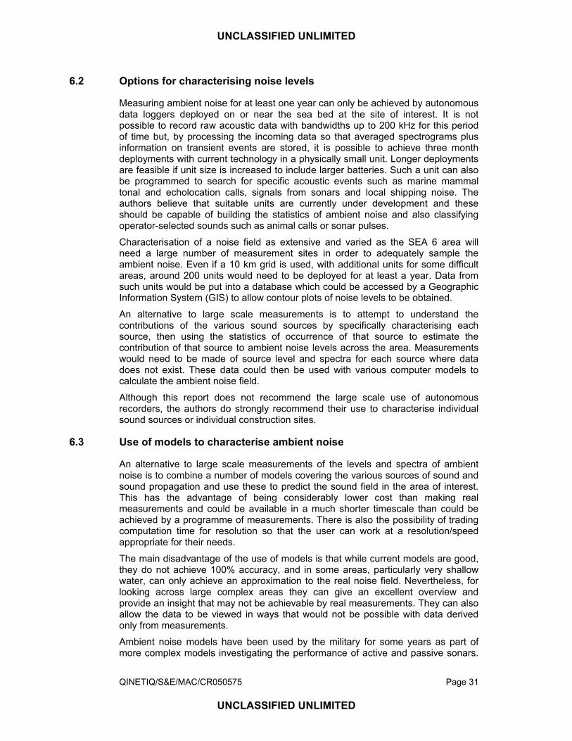
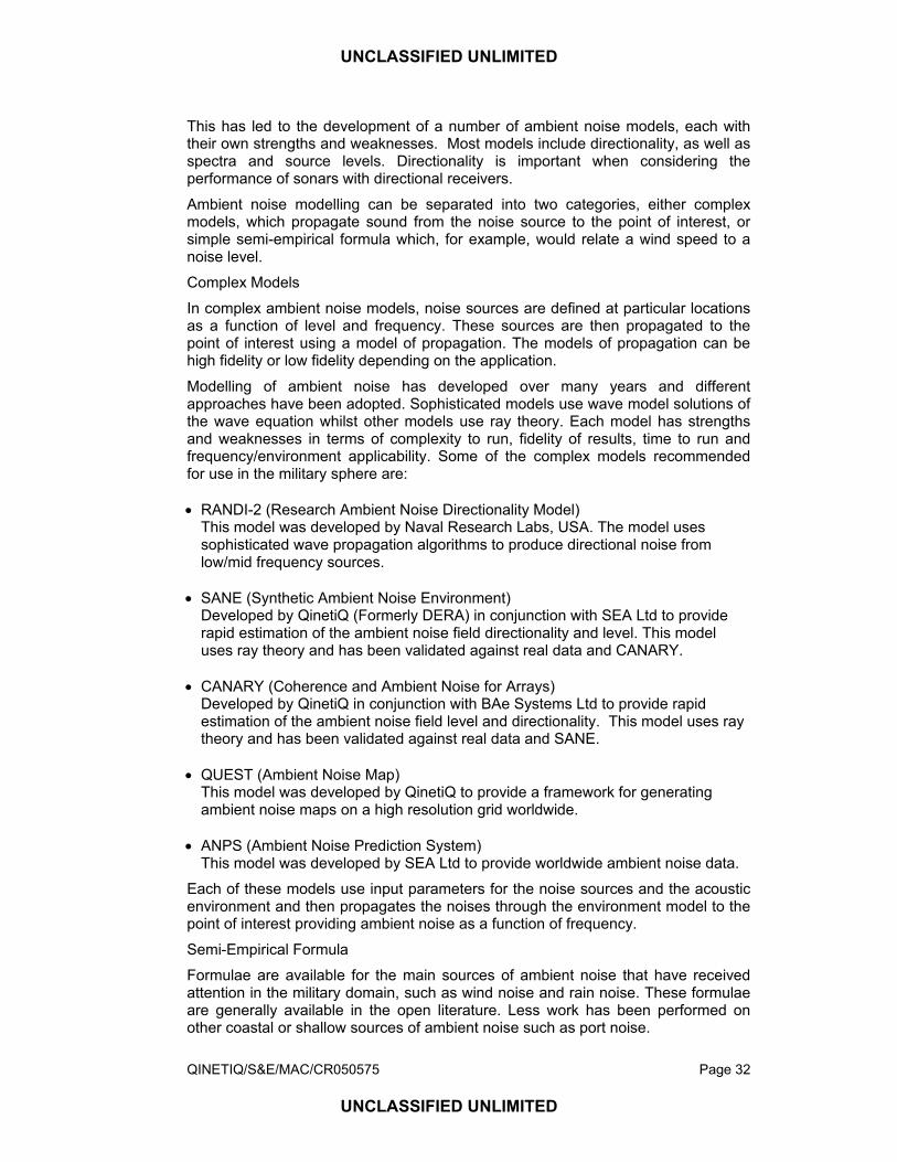
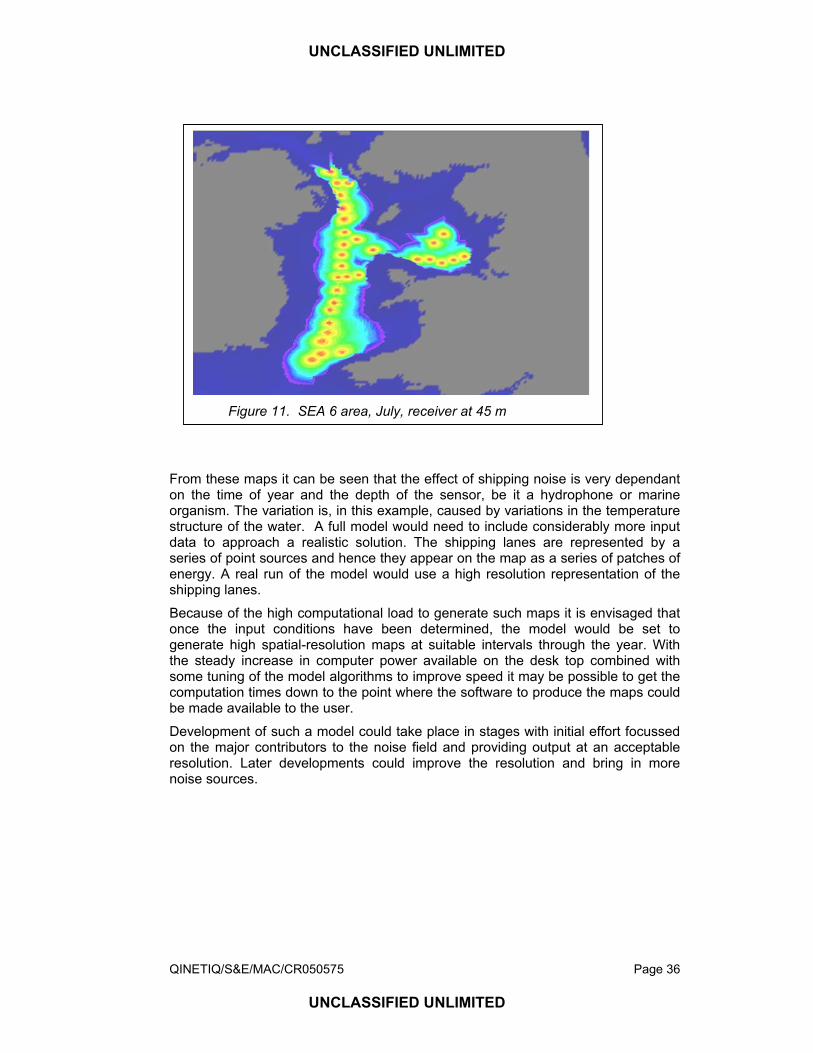
In order to demonstrate what could be achieved the QUEST model has been used to predict ambient noise maps for the SEA 6 area including shipping lanes through to Liverpool from the north and south of Ireland, gas rigs in Morecombe Bay and the Holyhead to Dublin Ferry route are shown in figures 7-10 for January, April, July and October respectively. For these figures the source is put at 5 metres depth and the receiver at 10 metres. In figure 11 the receiver is moved to 45 metres depth to give an indication of depth variation in the noise field. The red area is the highest ambient noise, while the blue area is the lowest level. It should be emphasised that these figures are to demonstrate what could be done with a noise model and not to provide accurate data. The sound field shapes at the extreme north and south are distorted by modelling artefacts.




Figure 7. SEA 6 area, January, receiver at 10 m

Figure 8.SEA 6 area, April, receiver at 10 m.




Figure 10. SEA 6 area, October, receiver at 10m

Figure 9. SEA 6 area, July, receiver at 10 m




From these maps it can be seen that the effect of shipping noise is very dependant on the time of year and the depth of the sensor, be it a hydrophone or marine organism. The variation is, in this example, caused by variations in the temperature structure of the water. A full model would need to include considerably more input data to approach a realistic solution. The shipping lanes are represented by a series of point sources and hence they appear on the map as a series of patches of energy. A real run of the model would use a high resolution representation of the shipping lanes.

Because of the high computational load to generate such maps it is envisaged that once the input conditions have been determined, the model would be set to generate high spatial-resolution maps at suitable intervals through the year. With the steady increase in computer power available on the desk top combined with some tuning of the model algorithms to improve speed it may be possible to get the computation times down to the point where the software to produce the maps could be made available to the user.

Development of such a model could take place in stages with initial effort focussed on the major contributors to the noise field and providing output at an acceptable resolution. Later developments could improve the resolution and bring in more noise sources.

Figure 11. SEA 6 area, July, receiver at 45 m




7 Identified information shortfalls

7.1 Natural sounds

Wind, waves and precipitation

Although there is still some doubt about the exact mechanisms by which noise is generated from these processes, there are a number of theoretical models available which give good agreement with measured levels and which can therefore be used to predict the level of contribution to ambient noise based on weather statistics.

A quick search for weather statistics for the SEA 6 area failed to find data with the level of detail needed to model the contribution of these sources.

Surf noise

The mechanics of noise generation in the surf zone are still not fully understood, but again there are a number of empirical models that give good agreement with measured levels and which can be used to predict sound levels. These models need weather statistics, sea and shore contour, and sediment information as input. There is also a need for a better understanding of the noise levels from rocky shorelines.

Sediment transport noise

Although the presence of sediment transport in the Eastern Irish Sea has been well documented, the contribution to ambient noise levels is not clear, and the presence of the noise source elsewhere in the SEA 6 area is also unclear.

Biological noise

No detailed maps of biological noise sources exist. Work is needed to identify the sound-producing species in the SEA 6 area. This should allow temporal and spatial distribution maps to be produced so that the level of contribution to ambient noise can be assessed. Since the sound-producing species are also likely to be the species most affected by increases in ambient noise levels this information will also assist later environmental impact studies.

7.2 Anthropogenic sounds

Aggregate extraction

There is no information on noise levels associated with this activity in the SEA 6 area. There is data for aggregate extraction in other areas but this needs to be obtained and collated. The limited time available to this study also prevented a full identification of all aggregate extraction activities within the SEA 6 area.

Shipping noise

This has been well studied over the years and shipping statistics for the SEA 6 area ports combined with acoustic propagation models will give a good assessment of noise fields within the SEA 6 area. Information on the tracks and numbers of ships using the smaller ports is needed to fully characterise shipping noise.




Leisure craft

No statistics exist for levels of leisure craft activity within the SEA 6 area. It may be possible to extrapolate the data gathered elsewhere by scaling for port size, but ideally a more controlled data gathering exercise is needed.

Industrial noise

Industrial noise has only been characterised in a very haphazard manner. Some aspects have been well documented, driven by specific environmental impact requirements, while others have not been documented at all. It would be particularly helpful to document the noise field around the SEA 6 area oil and gas fields and the operational wind farms. Power cable noise should be investigated, particularly with the growing number of wind farms likely to be operating in the area. Areas of high onshore industrial activity should be identified and measurements made of the noise coupled into the sea.

Military noise

It is unlikely that it will be possible to obtain information on military activities in the SEA 6 area. Acoustic data collection in the main exercise areas will give a good guide to the level of any contribution by such activities to ambient noise levels.

Sonar

No statistics on sonar usage exist for the SEA 6 area. This may well be a major contributor to ambient noise levels in some areas so a data gathering exercise could prove useful.

Aircraft noise

It has not been possible to identify aircraft movement statistics during this short study, but it is believed that fixed wing aircraft make a very small contribution to underwater ambient noise levels. However, the use of helicopters to service marine facilities is increasing and it would be useful to gather data on this activity in order to assess the level of the contribution this activity makes to ambient noise. The noise signature of the aircraft commonly in use also needs to be established.

Fishing activity

No information on trawl noise could be found during this study and it would be useful to make measurements of a range of trawls typical of those in use in the SEA 6 area. Detailed fishing statistics combined with information on sound levels would enable the contribution to ambient noise levels to be judged.




8 Recommendations It is recommended that the following method be used to characterise noise in the SEA 6 area:

a. Collect data on sound sources within the SEA 6 area in order to meet the shortfalls in information on these sources set out in section 7 above. Data should provide spectra, source levels and variability information for each source.

b. Collect information on the distribution and number of the sources to be included in a model of ambient noise.

c. Assemble the input data required to run the ambient noise model.

d. Modify an existing ambient noise model to operate in the required manner.

e. Run the model to provide the required noise field data. Depending on computation times this may be a set of pre-calculated plots or it may be on a ‘run as required’ basis.

f. Collect data from a selected number of sites within the SEA 6 area to validate the model.

g. Iterate the model to improve geographic resolution and include additional sources.

This programme of work will provide a good understanding of the ambient noise fields across a large proportion of the SEA 6 area. It will also provide information on how the field will vary with the different cycles affecting noise levels.

This work will complement the detailed measurements required to understand the ambient noise field at specific sites for possible construction activities. It is recommended that long term underwater acoustic monitoring of these specific construction sites, carried out to meet environmental impact requirements, be used to further refine the recommended modelling of the whole SEA 6 area noise field.




9 Conclusions This report has set out the sources of ambient noise likely to be found in the SEA 6 area. This information is based on the many years of experience built up within QinetiQ and its predecessor organisations while supporting research into military sonars.

Ambient noise is dependent on a wide range of physical, anthropogenic and natural sound sources. These sources add together in a complex manner resulting in significant spatial and temporal variations in the noise field. Thus short term measurements at a single location can only provide a snap-shot of the noise field and cannot be used to accurately extrapolate to other locations and times. To fully characterise the ambient noise field in the SEA 6 area requires multiple measurements at a large number of locations and across a period of a year.

A suggested alternative is to characterise each sound source and use this information with occurrence statistics for each source to model the ambient noise field across the SEA 6 area.




10 References Anon (1999) Ireland's marine and coastal areas and adjacent seas: An

environmental assessment. Marine Institute, Dublin.

Anon (2003) Singing propellers. Hydrocomp Inc, Report 138, Durham, NH, USA.

Bardyshev V., Velikanov A., Gershman S. (1971) Experimental studies of underwater noise in the ocean. Sov. Phys. Acoust. 16: 512-513.

Bass S., Hay A. (1997) Ambient noise in the natural surf zone: wave breaking frequencies. IEEE Journal of Oceanic Engineering 22: 411-424.

Buckingham M. J., Jones S. A. S. (1987) A new shallow-ocean technique for determining the critical angle of the seabed from the vertical directionality of the ambient noise in the water column. Journal of the Acoustic Society of America 81: 938-946.

Carey W., Browning D. (1988) Low frequency ocean ambient noise: Measurement and theory Natural mechanisms of surface generated noise in oceans. Kluwer Academic, Dordrecht, pp 361-376.

CEFAS (2003) Preliminary investigation of the sensitivity of fish to sound generated by aggregate dredging and marine construction. CEFAS, AE0914, Burnham-on-Crouch.

Clarke T. (2000) Prototype ambient noise directional array. UDT-2000

Danneskiold-Samsoe O. (2005) Offshore wind turbines: Underwater and airborne noise, Copenhagen, pp 1xA4.

Deane G. B. (1997) Sound generation and air entrainment by breaking waves in the surf zone. Journal of the Acoustic Society of America 102: 3151-3167.

Deane G. B. (1999) Acoustic hot-spots and breaking waves in the surf zone. Journal of the Acoustic Society of America 105: 3151-3167.

Deane G. B. (2000a) Long time-base observations of surf noise. Journal of the Acoustic Society of America 107: 758-770.

Deane G. B. (2000b) A model for the horizontal directionality of breaking wave noise in the surf zone. Journal of the Acoustic Society of America 107: 177-191

Desharnais F., Chapman D. F. M. (2002) Underwater measurements and modelling of a sonic boom. Journal of the Acoustic Society of America 111: 544-553.

Dowling A., Ffowcs-Williams J. (1983) Sound and sources of sound. Ellis Horwood, Chichester.

Franz G. (1959) Splashes as sources of sound in liquids. Journal of the Acoustic Society of America 31: 1080-1096.

Gibbons J. A. M. (2000) A review of the shipping traffic in the Durlston Marine Research Area 1997 to 2000. Durlston Marine Project, Swanage.

Glegg S. A. L., Olivieri M. P. (1999) Indian Rock Beach Experiment: Summary of results obtained with the Ambient Noise Sonar (ANS). Florida Atlantic University, Boca Raton, FL.




Glegg S. A. L., Pirie R., LaVigne A. (2000) A study of ambient noise in shallow water. Florida Atlantic University, Dania, FL.

Greene C. R., Jr. (1987) Characteristics of oil industry dredge and drilling sounds in the Beaufort Sea. Journal of the Acoustical Society of America 82: 1315-1324.

Haviland G. M., Sayigh L. S., Frankel A. S., Powell C. M., Bocconcelli A., Herman R. L. (2001) Mapping total environmental sound exposure of bottlenose dolphins, Tursiops truncatus, in the Wilmington, North Carolina Intracoastal Waterway. In: Holland RC (ed) OCEANS 2001. Marine Technology Society, Washington, pp 1392-1394.

Jones B. (1999) Raycalc and WAVECALC - A user guide. UCES, U99-8.

Jones L. A., Coyle M. D., Gilliland P. M., Larwood J. G., Murray A. R. (2004) The Irish Sea marine natural area profile: A contribution to regional planning and management of the seas around England. English Nature, Peterborough.

Jones S. A. S., Richards S. D. (2001) Ambient noise measurements in the surf zone. Proc IOA 23: 335-341.

Jones S. A. S., Richards S. D., Martin J. (2000) Ambient noise for surf zone characterisation Proceedings of the fifth European Conference on Underwater Acoustics, ECUA 2000. European Commission, Lyon, France, pp 717-722.

Knudsen V. O., Alford R. S., Emling J. W. (1948) Underwater ambient noise. Journal of Marine Research 7: 410.

Koay T. B., Potter J. R., Pallayil V., Tan E. T. (2002) PANDA; A rapidly deployable, self-recovering shallow water acquisition platform. MTS Sea Technology Magazine.

Koschinski S., Culik B. M., Henriksen O. D., Tregenza N., Ellis G., Jansen C., Kathe G. (2003) Behavioural reactions of free-ranging porpoises and seals to the noise of a simulated 2 MW windpower generator. Marine Ecology Progress Series 265: 263-273.

Li Z. (1998a) A practical method of surf forecasting. UCES, U98-10.

Li Z. (1998b) A three-dimensional numerical model of surface waves in the surf zone and longshore current generation over a plane beach. Estuarine, Coastal and Shelf Studies 47: 395-413.

Lighthill M. (1954) On sound generated aerodynamically II: Turbulence as a source of sound. Proc. R. Soc. London, Ser A. 222: 1-32.

Medwin H., Beaky M. M. (1989) Bubble sources of the Knudsen sea noise spectra. Journal of the Acoustic Society of America 86: 1124-1130.

Medwin H., Daniel A. C. (1990) Acoustical measurements of bubble production by spilling breakers. Journal of the Acoustic Society of America 88: 408-412.

Medwin H., Kurgan A., Nystuen J. A. (1990) Impact and bubble sound from raindrops at normal and oblique incidence. Journal of the Acoustic Society of America 88: 413-418.

Medwin H., Nystuen J. A., Jacobus P. W., Ostwald L. H., Snyder D. E. (1992) The anatomy of underwater rain noise. Journal of the Acoustic Society of America 92: 1613-1623.

Melville W. (1996) The role of surface-wave breaking in air-sea interaction. Annual Review of Fluid Mechanics 28: 279-321.




Melville W. K., loewen K., Lamarre E. (1993) Bubbles, noise and breaking waves: a review of laboratory experiments. In: Kerman BR (ed) Natural physical sources of underwater sound: sea surface sound. Kluwer Academic, pp 483-501.

Nedwell J., Langworthy J., Howell D. (2004) Assessment of sub-sea acoustic noise and vibration from offshore wind turbines and its impact on marine wildlife; initial measurements of underwater noise during the construction of offshore windfarms, and comparison with background noise. Subacoustech Ltd, 544 R 0424, Southampton.

Nystuen J. (1986) Rainfall measurements using underwater ambient noise. Journal of the Acoustic Society of America 74: 972-982.

Oguz H., Prosperetti A. (1990) Bubble entrainment by the impact of drops on liquid surfaces. Journal of fluid mechanics 219: 143-179.

Oguz H., Prosperetti A. (1993) Drop impact and the underwater noise of rain Natural physical sources of underwater sound. Kluwer Academic, Dordrecht, pp 669-682.

Prosperetti A. (1988) Bubble-related ambient noise in the ocean. Journal of the Acoustic Society of America 84: 1042-1054.

Pumphrey H., Crum L. (1988) Acoustic emission associated with drop impacts: Sea surface sound. Kluwer Academic, Dordrecht, pp 463-483.

Richards S., Heathershaw A., Thorne P. D. (1996) The effect of suspended particulate matter on sound attenuation in seawater. Journal of the Acoustic Society of America 100: 1447-1450.

Rowley S. J. (2004) Alpheus glaber. Pistol shrimp. Marine Life Information Network: Biology and sensitivity key information sub-programme. MARLIN web site. Marine Biological Association of the UK, Plymouth. www.marlin.ac.uk/species/Alpheusglaber.htm.

Scrimger J. A., Evans D. J., McBean G. A., Farmer D. M., Kerman B. R. (1987) Underwater noise due to rain, hail, and snow. Journal of the Acoustical Society of America 81: 79-86.

Smalldon G., Holthuis L. B., Fransen C. H. J. M. (1993) Coastal shrimps and prawns. Field Studies Council, Shrewsbury.

Thorne P. D. (1983) Laboratory and marine measurements on the acoustic detection of sediment transport. Journal of the Acoustic Society of America 80: 899-910.

Thorne P. D. (1985) The measurement of acoustic noise generated by moving artificial sediments. Journal of the Acoustic Society of America 78: 1013-1023.

Thorne P. D. (1993) Seabed saltation noise Natural physicsal sources of underwater sound. Kluwer Academic, Dordrecht, pp 721-744.

Urick R. J. (1972) Noise signature of an aircraft in level flight over a hydrophone in the sea. Journal of the Acoustical Society of America 52: 993-999.

Urick R. J. (1983) Principles of underwater sound. McGraw-Hill, New York.

Vincent M. A., Atkins S. M., Lumb C. M., Golding N., Liberknecht L. M., Webster M. (2004) Marine nature conservation and sustainable development - the Irish Sea Pilot. Joint Nature Conservation Committee, Peterborough.




Voglis G. M., Cook J. C. (1970) A New Source of Acoustic Noise observed in the North Sea. ULTRASONICS 8: 100-101.

Wenz G. M. (1962) Acoustic ambient noise in the ocean: Spectra and sources. Journal of the Acoustic Society of America 34: 1936-1955.

Wharam J. C., Gibbons J. A. M., Harland E. J. (2004) Potential impact of underwater noise on small cetaceans within the Durlston Marine Research Area 18th Annual conference of the European Cetacean Society. European Cetacean Society, Kolmarden, Sweden.

Wilson O. B., Stewart M. S., Wilson J. H., Bourke, R.H. (1997) Noise source level density due to surf - Part 1: Monterey Bay, CA. IEEE Journal of Oceanic Engineering 22: 425-433.

Wilson O. B., Wolf S. N., Ingenito F. (1985) Measurements of acoustic ambient noise in shallow water due to breaking surf. Journal of the Acoustic Society of America 78: 190-195.

Wursig B., Greene C. R., Jefferson T. A. (2000) Development of an air bubble curtain to reduce underwater noise of percussive piling. Marine Environmental Research 49: 79-93.




Initial distribution list External

Quentin Huggett Geotek Ltd

QinetiQ

Information Resources

T Clarke

C Fox

S G Healy

E J Harland

S A S Jones




Blank page




Report documentation page Originator’s Report Number QINETIQ/S&E/MAC/CR050575

Originator’s Name and Location E J Harland

QinetiQ, Winfrith

Customer Contract Number and Period Covered SEA6_Noise_QinetiQ, February-April 2005

Customer Sponsor’s Post/Name and Location

N/A

Report Protective Marking and any other markings

Date of issue Pagination No. of references

Unclassified Unlimited 15th March 2005 Cover + 47 59

Report Title

SEA 6 Technical report: Underwater ambient noise

Translation / Conference details (if translation give foreign title / if part of conference then give conference particulars)

N.A.

Title Protective Marking UNCLASSIFIED UNLIMITED

Authors E J Harland, S A S Jones & T Clarke

Downgrading Statement None

Secondary Release Limitations None

Announcement Limitations None

Keywords / Descriptors Ambient noise, SEA 6

Abstract

This report has been prepared by QinetiQ as part of the UK Department of Trade and Industry (Dti) offshore energy Strategic Environmental Assessment (SEA) programme. This technical report is part of the SEA 6 process which covers the area from Milford Haven northwards through St Georges Channel, the Irish Sea, The North Channel and up into the outer Clyde Estuary. This report looks at the sources of underwater noise that combine to provide the background ambient noise levels in the shallow waters of the SEA 6 area, considers the mechanisms by which the sound is generated and may then be modified by the environment. Options for characterising ambient noise levels in the SEA 6 area are presented.

Abstract Protective Marking: UNCLASSIFIED UNLIMITED

This form meets DRIC-SPEC 1000 issue 7




Blank page

Documents

SEA 6 Technical report: Underwater ambient noise - Gov.uk