i

National Snow and Ice Data Center ADVANCING KNOWLEDGE OF EARTH'S FROZEN REGIONS

Sea Ice In the Climate System A Russian View Special Report #16 13 March 2013

V.F. Zakharov State Research Center of the Russian Federation-Arctic and Antarctic Research Institute Federal Service for Hydrometeorology and Environment Monitoring St. Petersburg, Russian Federation

National Snow and Ice Data Center Cooperative Institute for Research in Environmental Sciences University of Colorado, Boulder, Colorado, USA

ii

iii

Contents

Contents ................................................................................................................................................................. iii Citation ............................................................................................................................................................... iii

Foreward ................................................................................................................................................................. v

Introduction ............................................................................................................................................................. 1

Geographical Distribution ....................................................................................................................................... 3

Horizontal Dimensions ........................................................................................................................................... 5

Thickness ................................................................................................................................................................ 9

Concentration ........................................................................................................................................................ 13

Age Categories ...................................................................................................................................................... 16

Intrasecular Ice Area Changes in the 20th Century. ............................................................................................. 19

Relationship of Thermal Conditions in the Atmosphere with the Development of Sea Ice ................................. 26

On Some Features of the Horizontal Development of Sea Ice Cover .................................................................. 32

Factors of Ice Formation and Melting .................................................................................................................. 35

Conditions in the Ocean and Sea Ice Development .............................................................................................. 37

Ice Cover Stability ................................................................................................................................................ 41

Sea Ice as a Factor of Climate Change ................................................................................................................. 45

Causes for Change in the Halocline Horizontal Dimensions ................................................................................ 50

Effect of the Arctic Ice on Atmospheric Circulation ............................................................................................ 56

Self-oscillation as a Moving Force for the Development of Natural Processes ................................................... 58

On the Nature of "Polar Forcing" ......................................................................................................................... 60

Conclusion ............................................................................................................................................................ 67

References ............................................................................................................................................................. 68

Citation

V.F. Zakharov. 1997. Sea Ice in the Climate System: A Russian View. NSIDC Special Report 16. Boulder CO, USA: National Snow and Ice Data Center. http://nsidc.org/pubs/special/nsidc_special_report_15.pdf.

iv

v

Forward

This report was distributed in 2000 as part of the EWG Sea Ice Atlas on CD-ROM [http://nsidc.org/data/g01962.html]. It is being re-published as an NSIDC Special Report in order to help ensure its preservation and broaden its distribution. It is presented here as it was published on the original Atlas, with only minor edits where the original translation was confusing and the correct meaning could be easily inferred.

The Environmental Working Group Arctic Atlases on CD-ROM resulted from an unprecedented U.S. – Russian collaboration [http://nsidc.org/noaa/ewg/index.html] that released military and other scientifically important data.

The full Atlas series contains information on the history of Russian and Western research in the Arctic; important, previously unavailable data for polar research; and several Russian language scientific papers translated into English.

- Florence Fetterer and Ann Windnagel, NSIDC, February 2013

1

Introduction

The cover of the Earth which includes the atmosphere, hydrosphere, upper layer of the lithosphere, cryosphere, and biosphere, in other words everything in the climate system that is in a constant state of development. An analysis of the changes occurring in all these spheres demonstrates their mutual relationships plus temporal and spatial consistency. Transformations of natural conditions on the Earth, beginning with comparatively small and ending with the enormous glacial-interglacial transformations of the Pleistocene, appear to be a direct result of the development of these processes.

The conditions necessary for the existence of the entire living world are very closely connected with these transformations. That is why it is extremely important to know in what direction and with what intensity the situation will develop in the near and more distant future. What factors are responsible for the occurring changes; what is their relative role and it is preserved with time? No answers to these questions have yet been found, and this cannot be ascertained without investigating the laws of climate system development, the moving force of the physical-geographical process. Numerous attempts to learn this have failed so far. The efforts have, however, contributed to a firm opinion on the leading role of climate in the physical-geographical process. The answers to the question on its nature were mainly sought through causes of climate change. The focus of investigators looking into these causes was directed to the factors, which could, in some or other way, change a thermodynamic state of the atmosphere. The changes in these properties, which occur constantly, can enhance or attenuate the solar radiation influx to the Earth’s surface and its loss of energy in the process of long-wave radiation. The dust content of the atmosphere an carbon dioxide level are among the primary factors which are able to noticeably affect the energy conducting properties of the atmosphere and, hence, the climate.

The certainty that CO2 and stratospheric aerosols affect thermal conditions contributed to their recognition as the most probable causes of climate change. However, it appeared that these factors were too insufficient to account for observed climate changes [30]. Lately, the most common belief is that the internal processes in the climate system can also be a cause of climate fluctuations.

In this case, the answer to what can be considered as the most probable regulator of the physical-geographical process can be found from analysis of the relationships between the components of the climate system. It is not necessary to investigate the cause-effect relationships between all these components in succession. It is sufficient to choose one of them, let us say sea ice, and consider its direct interaction with the atmosphere and the ocean – in the climate system and the significance of internal mechanisms in the natural process.

It should be noted that sea ice, which up to recently attracted the attention of only a narrow range of specialists, has become of wide scientific interest. It appears that among the physical elements constituting the climate system, sea ice and snow cover experience the most significant changes in time. This particular sensitivity of sea ice to comparatively small changes in the climate system in combination with the ease of tracking them with the help of modern space observation means has allowed us to choose it as a reliable indicator of climate change. By investigating how ice extent in the world’s oceans changes over time, we gain insight into the tendencies of global climate, i.e. the direction and intensity of the development of natural conditions on the Earth.

2

The climate significance of sea ice not, of course, only in its being a good indicator of climate change. Suffice it to say that the disappearance of ice in the Arctic, if it were possible, would result in an increase of mean annual temperature in its central regions by 15° C as compared with the current temperatures [7].

Sea ice appears to be the youngest component of the cryosphere. As is known, the first signs of the Cenozoic glaciation epoch appeared only about 38-26 million years ago in some regions of Antarctica. The formation of the Antarctic ice sheet began in the early Miocene, i.e. about 25-20 million years ago. As to the Northern Hemisphere, continental glaciation occurred much later. The earliest traces are found in the high mountains of Alaska, dated at 10 million (mln.) years (yr.). Although clear direct evidence about the time of the beginning of the development of the Greenland Ice Sheet is absent, it is believed that it also refers to the mid-Miocene. This sheet reached the dimensions, close to modern ones, about 3.5 mln. yr. It is from this time that the signs of glacial deposits appeared in deep marine sediments around Greenland. Sea ice appeared even later, about 0.7 mln. yr. ago, just yesterday from the geological viewpoint. It is of exceptional importance that this coincides with the beginning of glacial-interglacial fluctuations that accompanied the enormous transformations of nature on our planet. This coincidence only enhances an interest in sea ice and indicates a connection between these phenomena. Could it be that sea ice served as a last link, joining the elements into one whole chain and providing for the conversion of the climate system into the self-oscillation regime?

The work is devoted to the study of the Arctic climate system. In spite of the paucity of actual data, certain progress has been achieved over the last 10-15 years on the solution of this acute scientific problem, as indicated in publication [1,2,11,24,25,29,36,37] and numerous articles of scientists from the Institute (AARI). It should be remembered that these articles, for the first time, proved the importance of the disturbances not only of the current climate but also of the climate and natural conditions existing during the Pleistocene, the focus of attention of many scientists.

3

Geographical Distribution

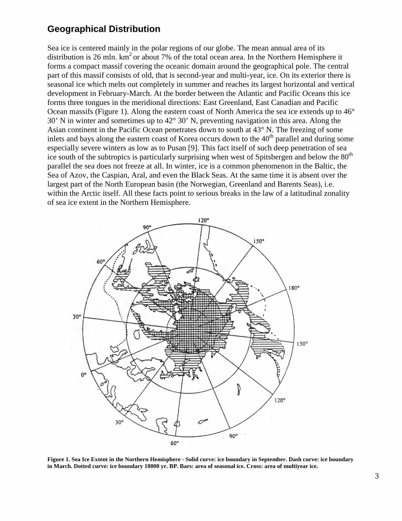
Sea ice is centered mainly in the polar regions of our globe. The mean annual area of its distribution is 26 mln. km2 or about 7% of the total ocean area. In the Northern Hemisphere it forms a compact massif covering the oceanic domain around the geographical pole. The central part of this massif consists of old, that is second-year and multi-year, ice. On its exterior there is seasonal ice which melts out completely in summer and reaches its largest horizontal and vertical development in February-March. At the border between the Atlantic and Pacific Oceans this ice forms three tongues in the meridional directions: East Greenland, East Canadian and Pacific Ocean massifs (Figure 1). Along the eastern coast of North America the sea ice extends up to 46° 30’ N in winter and sometimes up to 42° 30’ N, preventing navigation in this area. Along the Asian continent in the Pacific Ocean penetrates down to south at 43° N. The freezing of some inlets and bays along the eastern coast of Korea occurs down to the 40th parallel and during some especially severe winters as low as to Pusan [9]. This fact itself of such deep penetration of sea ice south of the subtropics is particularly surprising when west of Spitsbergen and below the 80th parallel the sea does not freeze at all. In winter, ice is a common phenomenon in the Baltic, the Sea of Azov, the Caspian, Aral, and even the Black Seas. At the same time it is absent over the largest part of the North European basin (the Norwegian, Greenland and Barents Seas), i.e. within the Arctic itself. All these facts point to serious breaks in the law of a latitudinal zonality of sea ice extent in the Northern Hemisphere.

Figure 1. Sea Ice Extent in the Northern Hemisphere - Solid curve: ice boundary in September. Dash curve: ice boundary in March. Dotted curve: ice boundary 18000 yr. BP. Bars: area of seasonal ice. Cross: area of multiyear ice.

4

In March, with an increase of solar energy, ice begins to destruct. The melting wave extends from the south, covering newer regions and reaching the North Pole in June. The exterior boundary retreats further north, the ice tongues become shorter, and the meridian typical of winter becomes weakly manifested by the end of summer. This indicates that the conditions inducing and maintaining the meridian in sea ice extent over the hemisphere are mainly pronounced during the coldest part of the year.

It should be noted that general features of the geographical ice distribution in the Northern Hemisphere correlate well with the character of surface oceanic circulation in polar and temperature latitudes. Its extent is southernmost along the eastern shores of Greenland, North America, and Asia where cold sea currents pass: the East Greenland, Labrador, and Oya-Shio. In the regions subjected to the effect of warm currents and, in particular some branches of the North Atlantic and Kuro-shio, the ice boundary retreats northward. This results in a strong asymmetry in the distribution of water temperature, salinity, and sea ice between the western and eastern Atlantic and Pacific Oceans. The formation of ice tongues is most often attributed to an automatic effect of sea currents and their ability to transport ice from one region to another, forgetting that the main ice mass composing these tongues has been formed at the place. Advection plays an insignificant role in the ice mass budget of the East Canadian and Pacific Ocean tongues. Ice transfer by cold sea currents cannot, therefore, be considered as the only or even the main factor of the meridian of ice extent in the Northern Hemisphere. A decisive condition necessary for ice formation in the regions subjected to the effect of cold currents appears, as will be shown below, to have the same thermohaline water structure which accompanies these currents.

Most of the Northern Hemisphere ice mass is drifting ice driven by wind and sea currents. The exception is the ice formed in shallow water areas near the shores which is attached and stationary. This is fast ice. In March, when this fast ice is most developed, its area from rough estimates is 1.8 mln. km2 in the Arctic Ocean alone. Fast ice is developed mostly in two regions: in the straits of the Canadian Arctic Archipelago and in shallow water surrounding the New Siberian Islands. The data from the end of the 1970s allow for a basic understanding of the development of shore fast ice in different parts of the ocean. According to these data, the area of stationary ice in spring reached the straits of the Canadian Arctic Archipelago- 0.809, around Greenland – 0.144, Spitsbergen – 0.038, Franz Josef Land – 0.033, Novaya Zemlya – 0.013, in the Kara Sea – 0.202, in the Laptev Sea – 0.208, in the East Siberian Sea – 0.254 mln. km2. Taking into account the fast ice surrounding the islands and the coast outside the Arctic Ocean, the total area of stationary ice in the hemisphere can be estimated to be approximately 2 mln. km2 which constitute 12% of the entire sea ice area during the annual maximum development. However, from this time, the fast ice area begins to steadily reduce. By the end of summer it is practically destroyed everywhere, either melting out on the spot or transformed into drifting ice.

5

Horizontal Dimensions

A very important parameter of sea ice appears to be its area. With time this area experiences changes, most global of which are seasonal, inter-annual and multi-year. The study of the changes themselves and the causes inducing them are considered to be one of the most important and interesting areas of sea ice research.

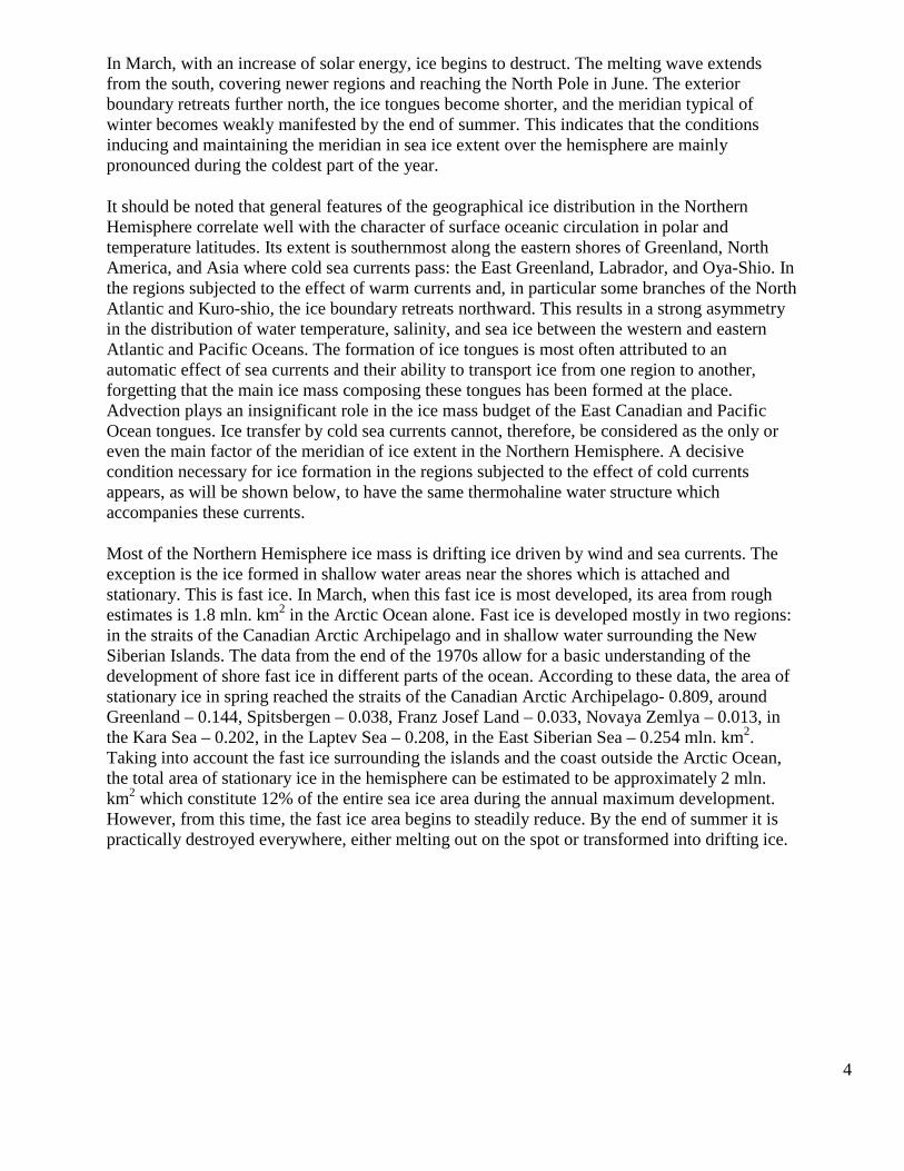
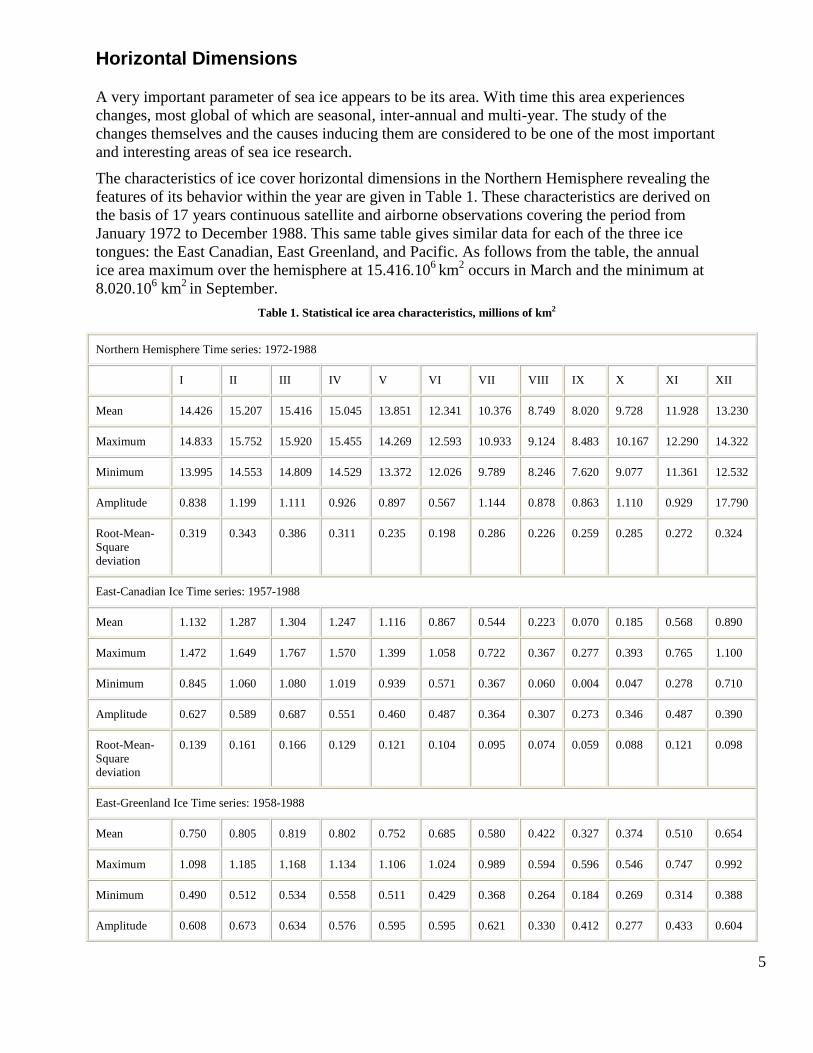
The characteristics of ice cover horizontal dimensions in the Northern Hemisphere revealing the features of its behavior within the year are given in Table 1. These characteristics are derived on the basis of 17 years continuous satellite and airborne observations covering the period from January 1972 to December 1988. This same table gives similar data for each of the three ice tongues: the East Canadian, East Greenland, and Pacific. As follows from the table, the annual ice area maximum over the hemisphere at 15.416.106 km2 occurs in March and the minimum at 8.020.106 km2 in September.

Table 1. Statistical ice area characteristics, millions of km2

Northern Hemisphere Time series: 1972-1988

I II III IV V VI VII VIII IX X XI XII

Mean 14.426 15.207 15.416 15.045 13.851 12.341 10.376 8.749 8.020 9.728 11.928 13.230

Maximum 14.833 15.752 15.920 15.455 14.269 12.593 10.933 9.124 8.483 10.167 12.290 14.322

Minimum 13.995 14.553 14.809 14.529 13.372 12.026 9.789 8.246 7.620 9.077 11.361 12.532

Amplitude 0.838 1.199 1.111 0.926 0.897 0.567 1.144 0.878 0.863 1.110 0.929 17.790

Root-Mean-Square deviation

0.319 0.343 0.386 0.311 0.235 0.198 0.286 0.226 0.259 0.285 0.272 0.324

East-Canadian Ice Time series: 1957-1988

Mean 1.132 1.287 1.304 1.247 1.116 0.867 0.544 0.223 0.070 0.185 0.568 0.890

Maximum 1.472 1.649 1.767 1.570 1.399 1.058 0.722 0.367 0.277 0.393 0.765 1.100

Minimum 0.845 1.060 1.080 1.019 0.939 0.571 0.367 0.060 0.004 0.047 0.278 0.710

Amplitude 0.627 0.589 0.687 0.551 0.460 0.487 0.364 0.307 0.273 0.346 0.487 0.390

Root-Mean-Square deviation

0.139 0.161 0.166 0.129 0.121 0.104 0.095 0.074 0.059 0.088 0.121 0.098

East-Greenland Ice Time series: 1958-1988

Mean 0.750 0.805 0.819 0.802 0.752 0.685 0.580 0.422 0.327 0.374 0.510 0.654

Maximum 1.098 1.185 1.168 1.134 1.106 1.024 0.989 0.594 0.596 0.546 0.747 0.992

Minimum 0.490 0.512 0.534 0.558 0.511 0.429 0.368 0.264 0.184 0.269 0.314 0.388

Amplitude 0.608 0.673 0.634 0.576 0.595 0.595 0.621 0.330 0.412 0.277 0.433 0.604

6

Root-Mean-Square deviation

0.142 0.156 0.167 0.148 0.127 0.123 0.119 0.088 0.088 0.075 0.114 0.154

Pacific Ice Time series: 1960-1989

Mean 1.443 1.909 2.071 1.749 0.822 0.197 0.030 0 0 0.003 0.173 0.699

Maximum 1.770 2.159 2.323 2.023 1.165 0.503 0.203 0 0 0.070 0.327 0.903

Minimum 1.125 1.536 1.782 1.290 0.543 0.038 0 0 0 0 0.079 0.532

Amplitude 0.645 0.623 0.541 0.733 0.622 0.465 0.203 0 0 0.070 0.248 0.371

Root-Mean-Square deviation

0.286 0.263 0.264 0.262 0.242 0.130 0.058 0 0 0.013 0.085 0.141

These and other values presented in the table differ a little from those obtained earlier data, were respectively 16.11⋅106 and 7.95⋅106 km2. Some data discrepancy appears, due to the use of different data series in calculations of mean values. Also excluded were the ice of the Baltic Sea, Sea of Azov, Caspian and Aral Seas which are isolated from the main massif. It should be noted that there are discrepancies in the data in foreign references. The reason is that different authors use different exterior boundary limits of the ice cover.

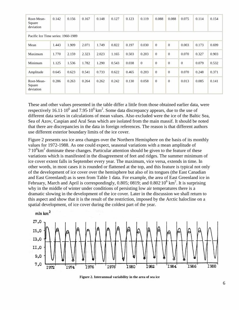
Figure 2 presents sea ice area changes over the Northern Hemisphere on the basis of its monthly values for 1972-1988. As one could expect, seasonal variations with a mean amplitude of 7.106km2 dominate these changes. Particular attention should be given to the feature of these variations which is manifested in the disagreement of feet and ridges. The summer minimum of ice cover extent falls in September every year. The maximum, vice versa, extends in time. In other words, in most cases it is rounded or flattened at the top, and this feature is typical not only of the development of ice cover over the hemisphere but also of its tongues (the East Canadian and East Greenland) as is seen from Table 1 data. For example, the area of East Greenland ice in February, March and April is correspondingly, 0.805; 0819; and 0.802.106 km2. It is surprising why in the middle of winter under conditions of persisting low air temperatures there is a dramatic slowing in the development of the ice cover. Later in the discussion we shall return to this aspect and show that it is the result of the restriction, imposed by the Arctic halocline on a spatial development, of ice cover during the coldest part of the year.

Figure 2. Interannual variability in the area of sea ice

7

In the same figure, circles denote seasonal maxima and minima of ice cover extent over the hemisphere form the Nimbus satellite data. One can see that these maxima in almost all cases appear to be a little less than our data. The variances in the minima are noticeably less. The reason of this is, probably, that the United States data do not take into account the ice of 1.5/10 concentration and less, usually confined to the marginal zone.

Table 1 also contains data which characterize the main features of spatial development of the East Canadian, East Greenland and Pacific ice tongues in the annual cycle. They are based on time scales of practically the same duration, covering approximately the last 30 years. One can see that the Pacific tongue, which includes ice of the Bering Sea and the Sea of Okhotsk, does not exist during the whole year. By the end of July ice in these seas melts out completely, appearing again only in October. Thus, the ice season along the Asian coast of our country lasts, on a average, about 10 months. The East Canadian ice tongue melts out almost completely by the end of summer. A small ice amount is preserved in the very north of Baffin Bay on the border with the straits. The East Greenland ice from winter to summer is reduced almost by 2.5 times, but it never melts out completely. This is the result of a constant ice supply exported from the Arctic basin. The picture of seasonal changes in the ice cover development in the Northern Hemisphere is supplemented and made more detailed by mean multiyear data on ice area in the marginal Arctic and ice infested seas given in Table 2. It does not include the seas, the ice of which appears to be a composite part of the ice tongues. It should also be remembered that the length of the series used for the calculations of the means is different, which is related more often with the discrepancies in the timing of the beginning of regular ice observations in different water reservoirs. Still, the data in a table form allow an understanding of the most important features of the annual cycle of ice development in the seas in all its diversity.

The time series used for the histograms have the same length as for the calculation of statistical characteristics in Table 1 and cover approximately the last 25 years.

Table 2. Mean ice area in the seas of the Northern Hemisphere, mln.km2

Sea Area I II III IV V VI VII VIII IX X XI XII

Barents 1.388 0.686 0.796 0.855 0.822 0.780 0.596 0.343 0.163 0.128 0.233 0.383 0.544

White 0.090 0.060 0.076 0.071 0.052 0.018 0 0 0 0 0 0 0.017

Kara 0.830 0.830 0.830 0.830 0.830 0.830 0.765 0.670 0.431 0.266 0.565 0.830 0.830

Laptev 0.536 0.536 0.536 0.536 0.536 0.536 0.482 0.423 0.281 0.196 0.510 0.536 0.536

East-Siberian 0.770 0.770 0.770 0.770 0.770 0.770 0.750 0.724 0.622 0.516 0.733 0.770 0.770

Chukchi 0.595 0.595 0.595 0.595 0.595 0.580 0.488 0.357 0.232 0.196 0.399 0.589 0.595

Beaufort 0.481 0.481 0.481 0.481 0.481 0.476 0.433 0.395 0.361 0.346 0.471 0.481 0.481

Hudson Bay 0.848 0.848 0.848 0.848 0.848 0.848 0.632 0.120 0 0 0.073 0.654 0.848

Azov 0.039 0.020 0.025 0.014 0.002 0 0 0 0 0 0 0 0.003

Caspian 0.394 0.068 0.065 0.049 0.017 0 0 0 0 0 0.005 0.018 0.046

8

Aral 0.066 0.040 0.052 0.041 0.010 0 0 0 0 0 0 0 0.011

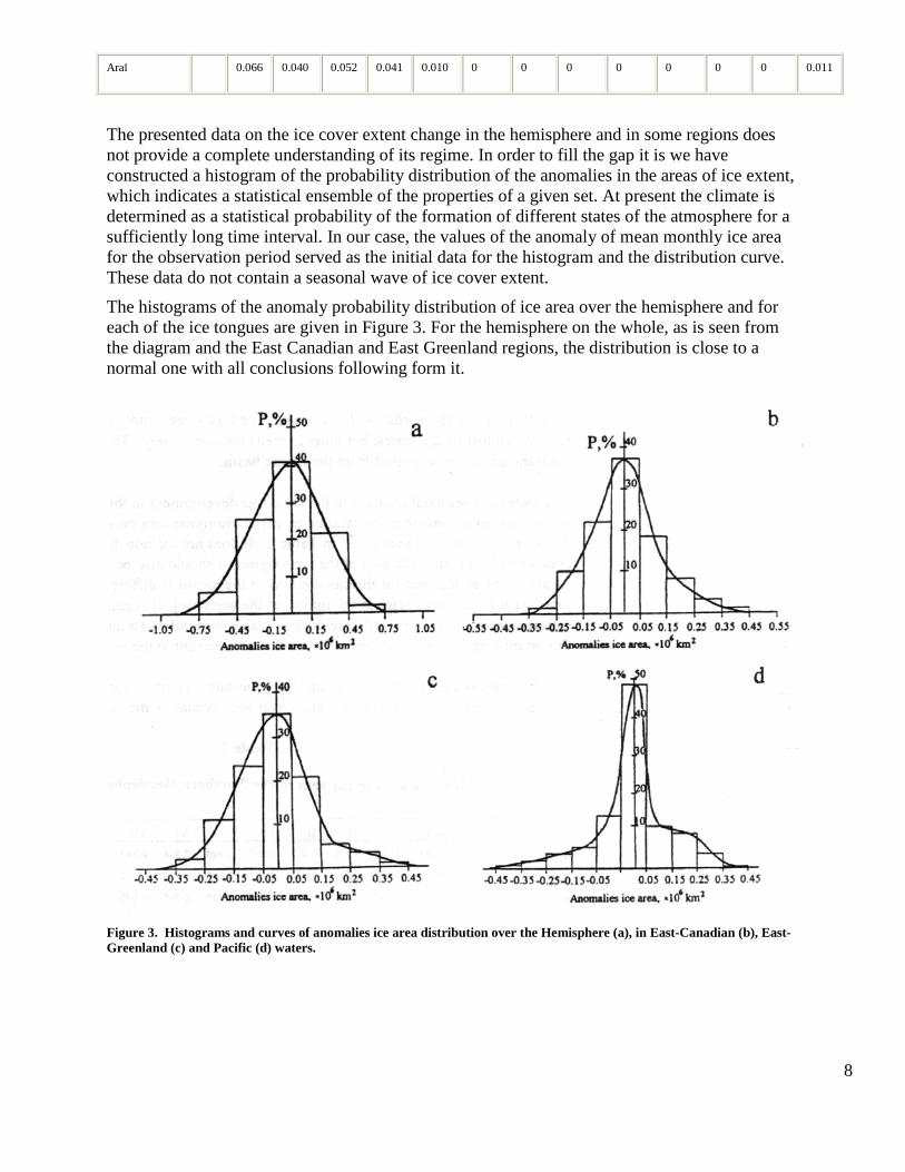
The presented data on the ice cover extent change in the hemisphere and in some regions does not provide a complete understanding of its regime. In order to fill the gap it is we have constructed a histogram of the probability distribution of the anomalies in the areas of ice extent, which indicates a statistical ensemble of the properties of a given set. At present the climate is determined as a statistical probability of the formation of different states of the atmosphere for a sufficiently long time interval. In our case, the values of the anomaly of mean monthly ice area for the observation period served as the initial data for the histogram and the distribution curve. These data do not contain a seasonal wave of ice cover extent.

The histograms of the anomaly probability distribution of ice area over the hemisphere and for each of the ice tongues are given in Figure 3. For the hemisphere on the whole, as is seen from the diagram and the East Canadian and East Greenland regions, the distribution is close to a normal one with all conclusions following form it.

Figure 3. Histograms and curves of anomalies ice area distribution over the Hemisphere (a), in East-Canadian (b), East-Greenland (c) and Pacific (d) waters.

9

Thickness

Thickness is considered to be the second most important characteristic of ice cover. Our knowledge about it has been inadequate in spite of much and steady interest from scientists and practical workers. This is partly due to a strong horizontal inhomogeneity in the thickness distribution and technical difficulties in measurement of its mass. The situation started to change quickly with the appearance of nuclear submarines equipped with sonars for searching the bottom ice surface. The first under ice voyage of such a submarine in the late 1950’s opened opportunities for the study of sea ice thickness for from the shores and was of primary importance. It served as a basis for the present day understanding of ice distribution over the Arctic Ocean. Since that time, it has become possible not only to collect a vast set of actual data, but also to create literature covering the aspects of methods for its processing and analysis and the scientific results proper on the ice thickness distribution in the routes of submarines. Data of contact measurements of fast ice thickness in the region of coastal stations and expeditions on drifting ice such as the Soviet "North Pole" stations or the British Transarctic expedition of 1969 have served as a basis for our present knowledge of the Arctic ice cover thickness. One should not forget that point measurements are, as a rule, not very much representative due to thickness variability. The reason for such thickness inhomogeneity even within a restricted area appears to be the amount of hummocking and an extreme diversity of floating ice with regard to the development stages.

With such a scattering of ice thickness, mass measurement by profile or area is required to obtain a statistically significant mean value. The length of such a profile for drifting ice, according to Wadhams [65], is from 50 to 100km.

In 1987 Bourke and Garrett published a work based on the data of underwater profiles northward of 65° N for 1960-1982 made by 17 submarines, which presents a generalized distribution pattern of mean thickness of the Arctic sea ice on the whole over the ocean in different seasons of the year. The total length of the underwater profiles used was about 200,000 km with the draft recorded every 1.5m. The accuracy of mean draft at the segments of 50 and 100 km was 0.3 – 0.5 m [51]. Let us use some results of this work to discuss large-scale ice distribution by thickness. Remember that the data in the work refer to the draft, i.e. part of the ice below water showed the draft to constitute 80-95% of its thickness. To pass from the draft to ice thickness, Wadhams suggests the use of an empirical coefficient of 1.12 [65].

It should also be remembered that the data by Bourke and Garrett on the draft were obtained without taking into account open water area in the ice cover. Due to this and some other reasons, the variations of ice thickness in the Arctic basin within a year do not reflect the change of its mass. At first glance and of a paradoxical nature, ice thickness in summer turns out to be thicker than in winter. Mean ice thickness for the Arctic Ocean in the fall (16.X – 15.I) was equal to 3.0, in winter (16.I – 15. IV) – 2.8m, in spring (16. IV – 15 VII) – 2.4 m and in summer (16. VII – 15.X) – 3.3. m. The increase of mean thickness from winter to summer from 2.8 to 3.3 m occurs due to the melting of young thin ice a persistence of thick old ice in the summer.

Mean annual draft on the whole for the Arctic Ocean is 2.9 m and the standard deviation is 1.8 m. The draft varies significantly from one region to another. This is illustrated by the data in Table 3. The thickest ice, as is seen from this table, is located in the Central Arctic, the Beaufort Sea and it the northern part of the straits of the Canadian Arctic Archipelago. The Kara sea and Baffin Bay, which become ice free in summer over a considerable area, are characterized by smaller thickness.

10

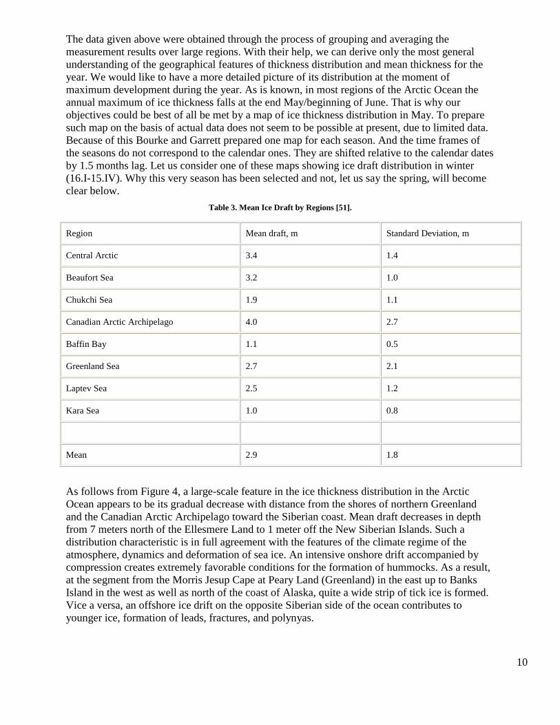
The data given above were obtained through the process of grouping and averaging the measurement results over large regions. With their help, we can derive only the most general understanding of the geographical features of thickness distribution and mean thickness for the year. We would like to have a more detailed picture of its distribution at the moment of maximum development during the year. As is known, in most regions of the Arctic Ocean the annual maximum of ice thickness falls at the end May/beginning of June. That is why our objectives could be best of all be met by a map of ice thickness distribution in May. To prepare such map on the basis of actual data does not seem to be possible at present, due to limited data. Because of this Bourke and Garrett prepared one map for each season. And the time frames of the seasons do not correspond to the calendar ones. They are shifted relative to the calendar dates by 1.5 months lag. Let us consider one of these maps showing ice draft distribution in winter (16.I-15.IV). Why this very season has been selected and not, let us say the spring, will become clear below.

Table 3. Mean Ice Draft by Regions [51].

Region Mean draft, m Standard Deviation, m

Central Arctic 3.4 1.4

Beaufort Sea 3.2 1.0

Chukchi Sea 1.9 1.1

Canadian Arctic Archipelago 4.0 2.7

Baffin Bay 1.1 0.5

Greenland Sea 2.7 2.1

Laptev Sea 2.5 1.2

Kara Sea 1.0 0.8

Mean 2.9 1.8

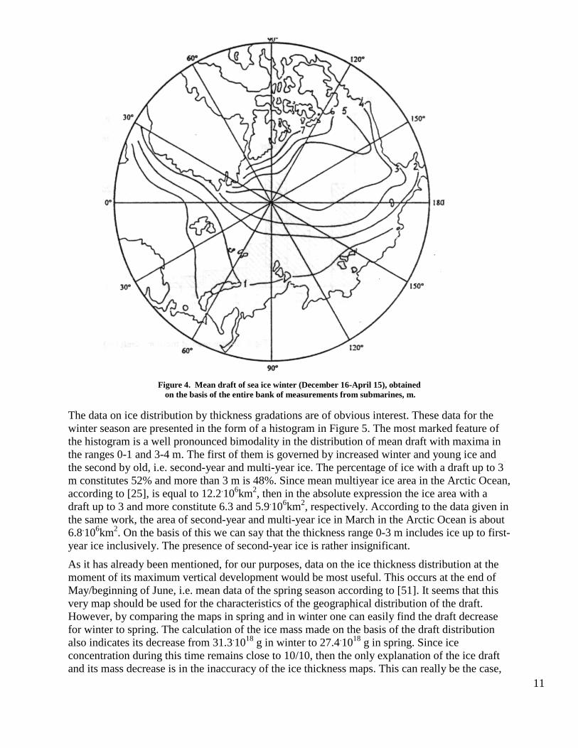
As follows from Figure 4, a large-scale feature in the ice thickness distribution in the Arctic Ocean appears to be its gradual decrease with distance from the shores of northern Greenland and the Canadian Arctic Archipelago toward the Siberian coast. Mean draft decreases in depth from 7 meters north of the Ellesmere Land to 1 meter off the New Siberian Islands. Such a distribution characteristic is in full agreement with the features of the climate regime of the atmosphere, dynamics and deformation of sea ice. An intensive onshore drift accompanied by compression creates extremely favorable conditions for the formation of hummocks. As a result, at the segment from the Morris Jesup Cape at Peary Land (Greenland) in the east up to Banks Island in the west as well as north of the coast of Alaska, quite a wide strip of tick ice is formed. Vice a versa, an offshore ice drift on the opposite Siberian side of the ocean contributes to younger ice, formation of leads, fractures, and polynyas.

11

Figure 4. Mean draft of sea ice winter (December 16-April 15), obtained

on the basis of the entire bank of measurements from submarines, m.

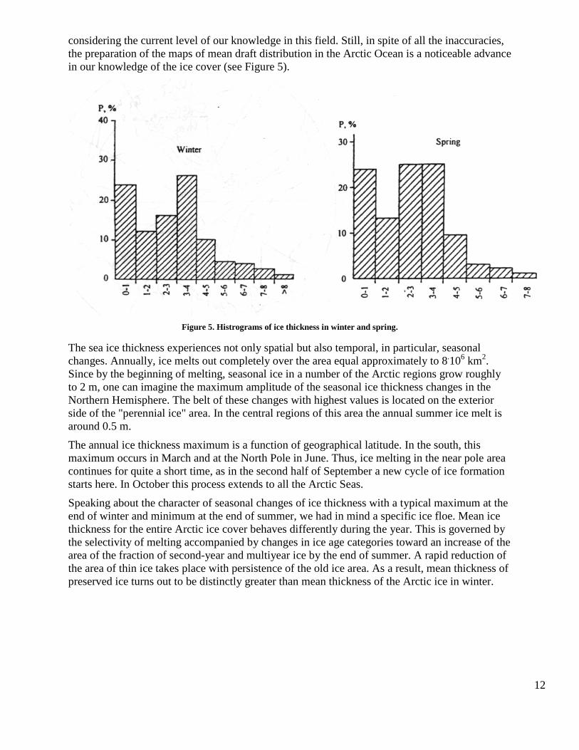
The data on ice distribution by thickness gradations are of obvious interest. These data for the winter season are presented in the form of a histogram in Figure 5. The most marked feature of the histogram is a well pronounced bimodality in the distribution of mean draft with maxima in the ranges 0-1 and 3-4 m. The first of them is governed by increased winter and young ice and the second by old, i.e. second-year and multi-year ice. The percentage of ice with a draft up to 3 m constitutes 52% and more than 3 m is 48%. Since mean multiyear ice area in the Arctic Ocean, according to [25], is equal to 12.2.106km2, then in the absolute expression the ice area with a draft up to 3 and more constitute 6.3 and 5.9.106km2, respectively. According to the data given in the same work, the area of second-year and multi-year ice in March in the Arctic Ocean is about 6.8.106km2. On the basis of this we can say that the thickness range 0-3 m includes ice up to first-year ice inclusively. The presence of second-year ice is rather insignificant. As it has already been mentioned, for our purposes, data on the ice thickness distribution at the moment of its maximum vertical development would be most useful. This occurs at the end of May/beginning of June, i.e. mean data of the spring season according to [51]. It seems that this very map should be used for the characteristics of the geographical distribution of the draft. However, by comparing the maps in spring and in winter one can easily find the draft decrease for winter to spring. The calculation of the ice mass made on the basis of the draft distribution also indicates its decrease from 31.3.1018 g in winter to 27.4.1018 g in spring. Since ice concentration during this time remains close to 10/10, then the only explanation of the ice draft and its mass decrease is in the inaccuracy of the ice thickness maps. This can really be the case,

12

considering the current level of our knowledge in this field. Still, in spite of all the inaccuracies, the preparation of the maps of mean draft distribution in the Arctic Ocean is a noticeable advance in our knowledge of the ice cover (see Figure 5).

Figure 5. Histrograms of ice thickness in winter and spring.

The sea ice thickness experiences not only spatial but also temporal, in particular, seasonal changes. Annually, ice melts out completely over the area equal approximately to 8.106 km2. Since by the beginning of melting, seasonal ice in a number of the Arctic regions grow roughly to 2 m, one can imagine the maximum amplitude of the seasonal ice thickness changes in the Northern Hemisphere. The belt of these changes with highest values is located on the exterior side of the "perennial ice" area. In the central regions of this area the annual summer ice melt is around 0.5 m.

The annual ice thickness maximum is a function of geographical latitude. In the south, this maximum occurs in March and at the North Pole in June. Thus, ice melting in the near pole area continues for quite a short time, as in the second half of September a new cycle of ice formation starts here. In October this process extends to all the Arctic Seas.

Speaking about the character of seasonal changes of ice thickness with a typical maximum at the end of winter and minimum at the end of summer, we had in mind a specific ice floe. Mean ice thickness for the entire Arctic ice cover behaves differently during the year. This is governed by the selectivity of melting accompanied by changes in ice age categories toward an increase of the area of the fraction of second-year and multiyear ice by the end of summer. A rapid reduction of the area of thin ice takes place with persistence of the old ice area. As a result, mean thickness of preserved ice turns out to be distinctly greater than mean thickness of the Arctic ice in winter.

13

Concentration

Concentration is also considered to be one of the most important ice cover characteristics. A large practical interest in it is quite reasonable because concentration, probably, governs to a greater extent than any other characteristic ice navigation conditions. However, it is similarly interesting in terms of pure science. The energy exchange between the ocean and the atmosphere in high latitudes in the regions of the usual ice cover extent depends to a great extent on its concentration. During the short summer open water areas appear to be "windows" through which solar energy penetrates the ocean and warms its upper layer. In winter there are also "windows" but for the heat flux in the opposite direction. In order to estimate these fluxes correctly and understand the importance of the Polar Ocean in the formation of the thermal atmospheric regime, it is necessary to know not only general features of the geographical distribution of concentration but also its time changes.

The most important feature of the change in concentration area appears to be its rapid increase deep into the massif. Over a small distance, as compared with the overall extent of the ice cover, it increases form 1-2/10 to 9-10/10. That is why it is not exaggeration to say that the Arctic ice cover presents an extensive area of close ice surrounded on the outside by a narrow open ice periphery. Although during the year the width of this periphery does not remain constant, it expands distinctly in summer and contracts in winter; it does not change the overall pattern. From the ice edge to its geometrical center close ice prevails even in summer.

The general character of seasonal changes in the ice cover concentration in the Arctic Ocean and separately in its deep sea region is quite fully disclosed by the data of Table 4. Monthly concentration values are obtained by recalculation of the data of Vowinckel an Orvig about the quantity of open water in the ice, given in [50]. They show that seasonal concentration changes in the Arctic Ocean do not exceed 0.3/10. Closer to the ice cover margins these changes increase up to 3.1/10. More pronounced seasonal changes of concentration in the marginal ocean part are related, first of all, with the more favorable conditions due to ice divergence and secondly with the prevalence of ice of younger development stages, which has time to melt out partly or completely during the warmer period of the year.

The data in the table indicate open water area in the ice. Thus, in the Arctic Basin the open water area in winter from November to June occupies only 1% of the total area. In summer it increases up to 4%. It is interesting to note that during the voyage of the U.S. nuclear submarines "Sargo" and "Sidrogen" in the Arctic Basin in January-March these areas constituted in total only 2% [57].

Wittmann and Schule [66] give higher values of total areas of open water in the wintertime as 5%. Swithenbank, who processed the data of the voyage of the British nuclear submarine "Dreadnought" the North Pole in March of 1971, found that the area occupied by open water and ice up to 0.5m thick constituted 5%, and that open water proper composed only a small part of this area [63]. According to data of Gorbunov, Borodachev and Shil’nikov, based on the generalization of visual airborne observations of February-May in the region between the coast of Siberia and the Pole, the area of young ice and open water varies from 1.5 to 4%. Wadhams data gathered on the 4,000 km route of the nuclear submarine "Sovereign" made during October 18-29 of 1976, the area of open water and ice up to 0.5 m thick varied from 0.2 to 15.6% with a mean value of 3.6%. Taking into account that the fraction of young ice in the fall is a little les than in winter it should be recognized that the result is in good agreement with the estimates made earlier.

14

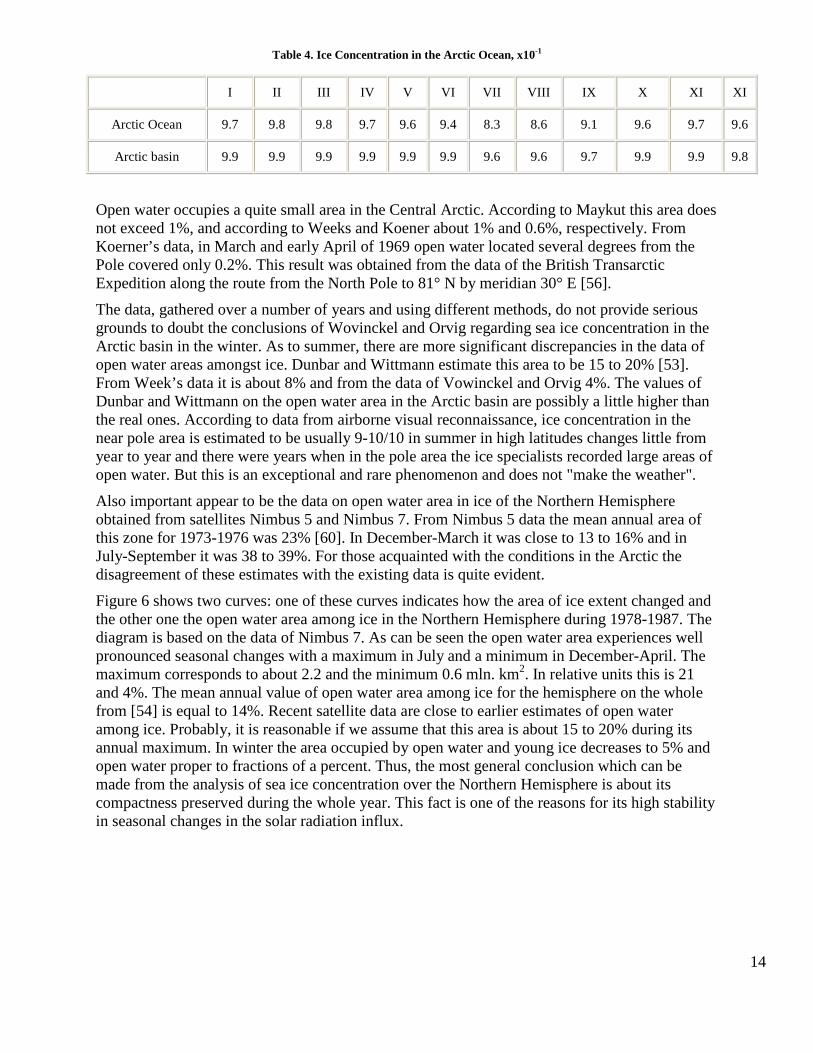
Table 4. Ice Concentration in the Arctic Ocean, x10-1

I II III IV V VI VII VIII IX X XI XI

Arctic Ocean 9.7 9.8 9.8 9.7 9.6 9.4 8.3 8.6 9.1 9.6 9.7 9.6

Arctic basin 9.9 9.9 9.9 9.9 9.9 9.9 9.6 9.6 9.7 9.9 9.9 9.8

Open water occupies a quite small area in the Central Arctic. According to Maykut this area does not exceed 1%, and according to Weeks and Koener about 1% and 0.6%, respectively. From Koerner’s data, in March and early April of 1969 open water located several degrees from the Pole covered only 0.2%. This result was obtained from the data of the British Transarctic Expedition along the route from the North Pole to 81° N by meridian 30° E [56].

The data, gathered over a number of years and using different methods, do not provide serious grounds to doubt the conclusions of Wovinckel and Orvig regarding sea ice concentration in the Arctic basin in the winter. As to summer, there are more significant discrepancies in the data of open water areas amongst ice. Dunbar and Wittmann estimate this area to be 15 to 20% [53]. From Week’s data it is about 8% and from the data of Vowinckel and Orvig 4%. The values of Dunbar and Wittmann on the open water area in the Arctic basin are possibly a little higher than the real ones. According to data from airborne visual reconnaissance, ice concentration in the near pole area is estimated to be usually 9-10/10 in summer in high latitudes changes little from year to year and there were years when in the pole area the ice specialists recorded large areas of open water. But this is an exceptional and rare phenomenon and does not "make the weather".

Also important appear to be the data on open water area in ice of the Northern Hemisphere obtained from satellites Nimbus 5 and Nimbus 7. From Nimbus 5 data the mean annual area of this zone for 1973-1976 was 23% [60]. In December-March it was close to 13 to 16% and in July-September it was 38 to 39%. For those acquainted with the conditions in the Arctic the disagreement of these estimates with the existing data is quite evident.

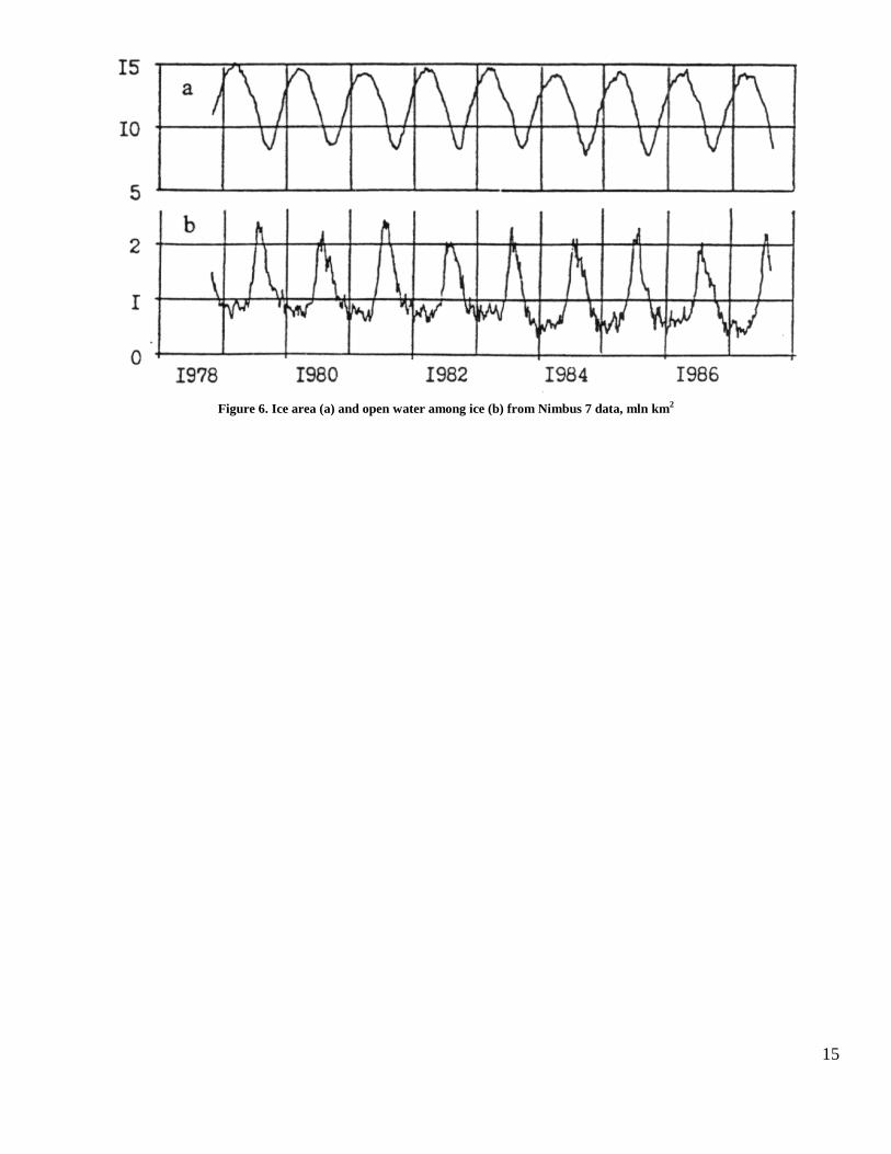
Figure 6 shows two curves: one of these curves indicates how the area of ice extent changed and the other one the open water area among ice in the Northern Hemisphere during 1978-1987. The diagram is based on the data of Nimbus 7. As can be seen the open water area experiences well pronounced seasonal changes with a maximum in July and a minimum in December-April. The maximum corresponds to about 2.2 and the minimum 0.6 mln. km2. In relative units this is 21 and 4%. The mean annual value of open water area among ice for the hemisphere on the whole from [54] is equal to 14%. Recent satellite data are close to earlier estimates of open water among ice. Probably, it is reasonable if we assume that this area is about 15 to 20% during its annual maximum. In winter the area occupied by open water and young ice decreases to 5% and open water proper to fractions of a percent. Thus, the most general conclusion which can be made from the analysis of sea ice concentration over the Northern Hemisphere is about its compactness preserved during the whole year. This fact is one of the reasons for its high stability in seasonal changes in the solar radiation influx.

15

Figure 6. Ice area (a) and open water among ice (b) from Nimbus 7 data, mln km2

16

Age Categories

The sea ice cover is rather non uniform by age category. This is due to recently formed or new ice, so called nilas; young and first-year ice of different development stages; and old including multiyear ice. A relative amount of each ice type changes over time and from region to region. In the ice cover melting phase ice of later formation disappears completely and melts out. The most stable part of the ice cover appears to be multiyear and second-year ice and is centered mainly in the central Arctic Ocean. This is the core of the polar cap of our hemisphere. Its mean multiyear area constitutes about 6.8 mln. km2 or 42% of the total ice area in March. Please note that in this section we speak about ice of 10/10 concentration. Such data characterize the amount of ice at different age categories, rather than the dimensions of the location area.

On the edges of the core there is first-year ice. Its formation starts among the remaining ice in September. In October, ice formation extends into the regions of open water and then from month to month it extends further southward, forming a belt of first-year ice (Figure 1). It exceeds that of old ice as early as March.

First-year ice is replaced by young ice at the boundary with open water. According to the existing nomenclature [39] this ice includes nilas, grey and grey-white ice not more than 30 cm thick. Since at such a thickness the vertical ice growth is quite intensive, young ice extends to the polar cap edge, contouring it over the entire perimeter in the form of a narrow band.

Thus, the general feature of the geographical distribution of sea ice by age categories is that it becomes younger the greater the distance from the core. Since the age categories indirectly indicate the thickness of the ice cover, it means that this cover is like a gigantic lens with the center in the Arctic basin.

Of course, the real pattern of sea ice distribution by age over the hemisphere is more complex. As a result of the wind and current driven ice displacement, the contours of the region, where the ice of a given age is centralized, attain features corresponding to the prevailing drift system. Due to this, multiyear ice is observed not only in the Arctic basin itself, but also the eastern coast of Greenland up to Farvel Cape, i.e. far from the region of its formation.

In the seas of the Far East where the ice age limit is one year, the ice thickness increases not only in the northern but also in the western direction. Near the shores of Asia ice formation begins earlier and more intensively than in the open sea. In the Arctic seas, extensive zones of young ice can sometimes be encountered among older ice, etc. However, all this complicates the pictures but does not obscure the main point of the increase of ice age with latitude.

Table 5 presents quantitative data on the development of ice different age categories at the maximum extent of the ice cover (March). The details of the age category proper of first-year ice are given by the formation time and not by thickness.

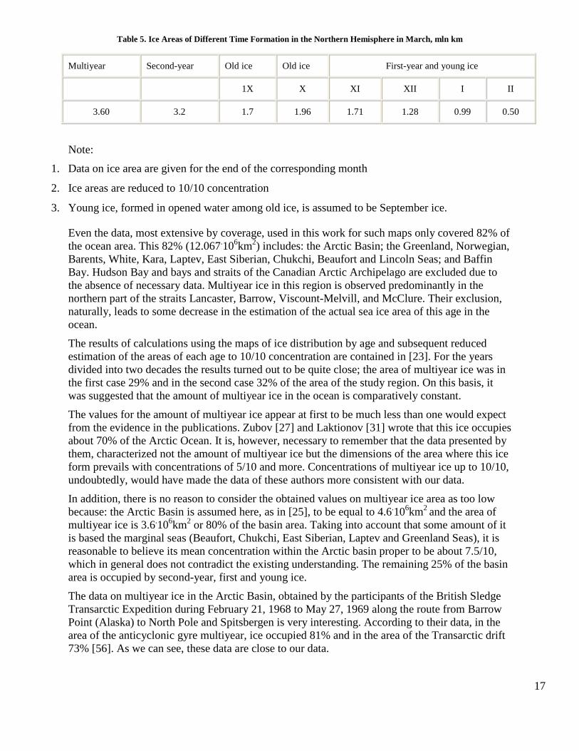
The area of multiyear ice, equal to 3.6.106km2 is obtained from two maps of ice conditions in the Arctic basin and marginal seas referring to the mid 50’s and 70’s of this century. The ice observations were carried out sufficiently regularly, mainly in the coastal ocean area which was important in terms of navigation. As to the observations over the remaining region, they are not only extremely irregular but too incomplete to compile maps of ice distribution by age categories.

17

Table 5. Ice Areas of Different Time Formation in the Northern Hemisphere in March, mln km

Multiyear Second-year Old ice Old ice First-year and young ice

1X X XI XII I II

3.60 3.2 1.7 1.96 1.71 1.28 0.99 0.50

Note:

1. Data on ice area are given for the end of the corresponding month

2. Ice areas are reduced to 10/10 concentration

3. Young ice, formed in opened water among old ice, is assumed to be September ice.

Even the data, most extensive by coverage, used in this work for such maps only covered 82% of the ocean area. This 82% (12.067.106km2) includes: the Arctic Basin; the Greenland, Norwegian, Barents, White, Kara, Laptev, East Siberian, Chukchi, Beaufort and Lincoln Seas; and Baffin Bay. Hudson Bay and bays and straits of the Canadian Arctic Archipelago are excluded due to the absence of necessary data. Multiyear ice in this region is observed predominantly in the northern part of the straits Lancaster, Barrow, Viscount-Melvill, and McClure. Their exclusion, naturally, leads to some decrease in the estimation of the actual sea ice area of this age in the ocean.

The results of calculations using the maps of ice distribution by age and subsequent reduced estimation of the areas of each age to 10/10 concentration are contained in [23]. For the years divided into two decades the results turned out to be quite close; the area of multiyear ice was in the first case 29% and in the second case 32% of the area of the study region. On this basis, it was suggested that the amount of multiyear ice in the ocean is comparatively constant.

The values for the amount of multiyear ice appear at first to be much less than one would expect from the evidence in the publications. Zubov [27] and Laktionov [31] wrote that this ice occupies about 70% of the Arctic Ocean. It is, however, necessary to remember that the data presented by them, characterized not the amount of multiyear ice but the dimensions of the area where this ice form prevails with concentrations of 5/10 and more. Concentrations of multiyear ice up to 10/10, undoubtedly, would have made the data of these authors more consistent with our data.

In addition, there is no reason to consider the obtained values on multiyear ice area as too low because: the Arctic Basin is assumed here, as in [25], to be equal to 4.6.106km2 and the area of multiyear ice is 3.6.106km2 or 80% of the basin area. Taking into account that some amount of it is based the marginal seas (Beaufort, Chukchi, East Siberian, Laptev and Greenland Seas), it is reasonable to believe its mean concentration within the Arctic basin proper to be about 7.5/10, which in general does not contradict the existing understanding. The remaining 25% of the basin area is occupied by second-year, first and young ice.

The data on multiyear ice in the Arctic Basin, obtained by the participants of the British Sledge Transarctic Expedition during February 21, 1968 to May 27, 1969 along the route from Barrow Point (Alaska) to North Pole and Spitsbergen is very interesting. According to their data, in the area of the anticyclonic gyre multiyear, ice occupied 81% and in the area of the Transarctic drift 73% [56]. As we can see, these data are close to our data.

18

In addition to what has already been said above the amount of multiyear ice in the Arctic Ocean one can add the following. From the estimate of Borodachev ( 1978) this amount in the areal expression for summertime is 3.6.106km2, not including the straits of the Canadian Arctic Archipelago. From Lebedev’s data of 1981 it constituted 3.4.106km2. According to calculations of Mironov (1984) the area of multiyear ice in the Arctic basin and the marginal seas, with the exception of the Greenland Sea, from September to June changes from 3.63 to 3.08.106km2. All of these estimates are quite consistent with each other, which indicate a sufficient level of our knowledge on the development of multiyear ice in the Arctic Ocean at present time.

According to Table 5, the area of second-year ice in the Arctic Ocean, reduced to 10/10 concentration, constitutes 3.2.106km2. This value is obtained from actual data by means of calculations based on the following. Obviously, the old ice area in the hemisphere in winter generally corresponds to the area of the so called remaining ice at the beginning of the new ice formation cycle, i.e.in September. From data in Table 1, this area is 8 mln. km2. Taking into account a concentration of remaining ice equal to 8.6/10, its reduced area will be 6.8.106km2. During winter the area of this ice due to the absence of melting remains constant, there is only regrouping. With known area of multiyear ice, it will not be difficult to determine the amount of second-year ice. The value, found in this way, is given in Table 5. It should be mentioned that it quite evidently differs from the one given by Mironov (1.47-1.27.106km2).

Thus, the ice cover of the Northern Hemisphere during the period of its maximum development, i.e. in March, consists of 22% of multiyear ice, 20% of second-year ice and 58% of first-year and young ice. Taking into account a rapid growth of ice of small thicknesses, we believe that the young ice share in the total mass balance is not significant. We also state that the high level of present day knowledge on seasonal variability of the ice cover development in the hemisphere allows us to consider as quite reliable the date on the total amount of old and first-year ice formed during current winter. As to the portion of second-year ice, its estimation is possible by means of a more accurate assessment of ice concentration at the beginning of the new ice formation cycle.

Multiyear ice, undoubtedly, is the most vivid feature of the ice cover of the Arctic Ocean. It is centered in the near pole area, however the source of its formation is shifted toward Greenland and the Canadian Arctic Archipelago, being related to area of the anticyclonic gyre of surface water and ice. The eye of this gyre is located approximately at the point of 78° N, 150° W. The ice involved in this gyre cannot be exported out to the Arctic basin for many years. According to the calculations of Vowinckel [50] about 2% of the area of this basin is occupied by ice, the age category of which is about 19 years. Naturally this ice differs distinctly from multiyear ice north of the coast of Siberia, even in appearance.

At the periphery of the anticyclonic gyre and in the system of the Transarctic Current crossing the Arctic Ocean from the Chukchi Sea across the North Pole to Fram Stait multiyear ice by thickness is less than the Canadian one. In accordance with the features of surface water and ice circulation, it either has branches in the southern direction and approaches the coast, as in the East Siberian Sea, or vice versa retreats far from the shores. In the first case, it creates considerable difficulties for navigation even during the most favorable time of the year. That is why any shift of the multiyear ice boundary to the southern direction affects not only ice conditions but navigation as well.

19

Intrasecular Ice Area Changes in the 20th Century.

For a long monitoring of the Arctic ice cover as one whole body was impossible due to its vast dimensions, comparable with those of some mainlands. Observation on the volume meeting the interest and focus of each separate Arctic State were carried out in some parts of the marginal zone of the gigantic ice "pancake". Yet by the early 1960s the observations extended to the marginal zone over practically the entire perimeter of the ice cover of the Northern Hemisphere, covering the largest part of the annual cycle of its development. Since the synchronization of the observations was rather unsatisfactory, the data on the horizontal dimensions of this cover could be obtained only with a monthly interval. With the onset of the "satellite epoch" the data obtained from meteorological satellites became an important information source on sea ice. The data from the second half of the 1960s supplemented the ice data obtained by traditional methods and, on the whole, increased the quality of ice data. However, a strong dependence of the first satellites on cloud and illumination conditions governed the irregularity of satellite ice information. It was possible to overcome this shortcoming in the 1970s when satellites were launched into the Earth’s orbit making ice observations independent of these conditions. The possibility to obtain ice information on a global scale with time interval of several days appeared. And science for the first time was able to trace polar ice development in the far north and south or our planet almost simultaneously.

Up to the early 1960s data collected from aircraft, ships, and coastal stations. They were of a regional character. The quality of these data is different, on the whole less reliable the older it is. The wide use of aviation for ice observations north of the coast of Siberia began in the late 30s and the North American Arctic waters in mid 1950s. Up to that time the observations from a few stations, fishing, transport and expedition vessels served as the source of evidence on the ice in the Arctic. The observations of ice extent in the seas of the Siberian shelf constitute the longest data series (from 1924) characterizing ice conditions over an extensive area (from Novozemel’sky straits to Bering Strait). Up to 1932, however, it covers only a narrow interval of the seasonal cycle, the second half of August. Since 1932, i.e. since the voyage of the "Sibiryakov" which started the epoch of transport exploration of the Northern Sea Route, the ice observations extended to July, August and September and since 1946 to the entire summer navigation with a detailed description by 10 day periods. The reliability of the series is not consistent: the data from 1924-1931 can arbitrarily be considered as rough data, those from 1932-1945 as sufficiently reliable and the remaining portion as quite reliable.

The data on the ice state in the Atlantic sector of the Arctic (Davis Strait, the Labrador Sea, the eastern Greenland waters and the Barents Sea) were systematized and generalized by the Danish Meteorological Institute in the form of monthly maps for April-August of 1901-1956 [55]. The data can be considered as approximate data as they are based on shipborne observations recording the geographical position of some points of sea ice limits in different days of the month. However, one should not underestimate their significance as only they present a real picture of ice conditions of the first half of the 20th century.

A systematic study of ice conditions in the North American Arctic waters started in the second half of the 1950’s. The same can be said about ice jammed seas of the northern Pacific Ocean (the Bering, Okhotsk Seas and in the northernmost regions of the Sea of Japan). In winter the Pacific Ocean ice joins in the narrow Bering Strait with the Arctic ice, forming one extended ice cover of a complicated configuration. In summer the Pacific ice melts out completely and the need to trace it disappears. Completing the characteristics of initial data on the Arctic sea ice

20

extent during 20th century, it should be admitted that these data are rather inconsistent both in quantity and quality.

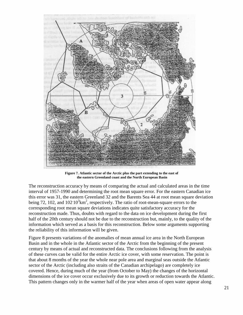
The duration of the series of data on mean annual areas of the Arctic sea ice is restricted to the last 30 to 35 years. This is only one third of the period of instrumental observations of surface air temperature in the hemisphere. Taking this into account it seems natural to attempt to reconstruct the mean annual values of the area of the Arctic ice on the basis of incomplete data. There is possibility for such a reconstruction from the beginning of the current century for a number of the regions of the Arctic Ocean: East Canadian region (Baffin Bay, Labrador Sea and Davis Strait), East Greenland region (south of 80° N parallel up to Farvel Cape), and the Norwegian and Barents Seas. All this area will be further called the Atlantic sector of the Arctic plus the part extending to the east of the eastern Greenland coast and the North European Basin (Figure 7). The reconstruction of the mean annual ice areas in each of the regions listed is based on the areas averaged for April-August from the observation data. The calculation equations for the transition from the mean seasonal to the mean annual area are found from data for 1960-1989, that is for the period with a full data set covering the entire annual evolution cycle.

East Canadian region Y1 = 0.78 X1 + 163, r = 0.90 + 0.03;

East Greenland region Y1 = 0.90 X2 + 163, r = 0.96 + 0.01;

And the Barents Sea Y3 = 0.96 X3 + 91, r = 0.92 + 0.02.

where: Y1, Y2, Y3 respectively represent mean annual ice areas in the East Canadian, East Greenland regions and the Barents Sea; X1, X2 = mean ice area for April-August in the East Canadian and the East Greenland regions, X3 = mean ice area for May-August in the Barents Sea.

21

Figure 7. Atlantic sector of the Arctic plus the part extending to the east of

the eastern Greenland coast and the North European Basin

The reconstruction accuracy by means of comparing the actual and calculated areas in the time interval of 1957-1990 and determining the root mean square error. For the eastern Canadian ice this error was 31, the eastern Greenland 32 and the Barents Sea 44 at root mean square deviation being 72, 102, and 102.103km2, respectively. The ratio of root-mean-square errors to the corresponding root mean square deviations indicates quite satisfactory accuracy for the reconstruction made. Thus, doubts with regard to the data on ice development during the first half of the 20th century should not be due to the reconstruction but, mainly, to the quality of the information which served as a basis for this reconstruction. Below some arguments supporting the reliability of this information will be given.

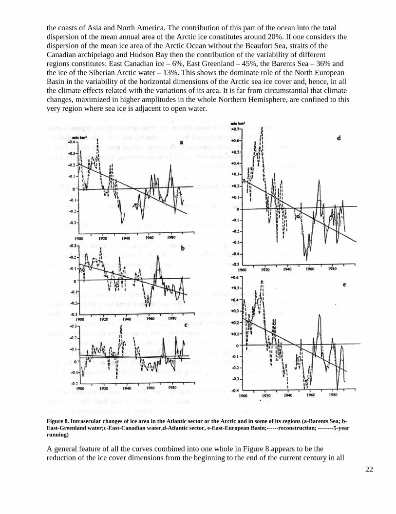
Figure 8 presents variations of the anomalies of mean annual ice area in the North European Basin and in the whole in the Atlantic sector of the Arctic from the beginning of the present century by means of actual and reconstructed data. The conclusions following from the analysis of these curves can be valid for the entire Arctic ice cover, with some reservation. The point is that about 8 months of the year the whole near pole area and marginal seas outside the Atlantic sector of the Arctic (including also straits of the Canadian archipelago) are completely ice covered. Hence, during much of the year (from October to May) the changes of the horizontal dimensions of the ice cover occur exclusively due to its growth or reduction towards the Atlantic. This pattern changes only in the warmer half of the year when areas of open water appear along

22

the coasts of Asia and North America. The contribution of this part of the ocean into the total dispersion of the mean annual area of the Arctic ice constitutes around 20%. If one considers the dispersion of the mean ice area of the Arctic Ocean without the Beaufort Sea, straits of the Canadian archipelago and Hudson Bay then the contribution of the variability of different regions constitutes: East Canadian ice – 6%, East Greenland – 45%, the Barents Sea – 36% and the ice of the Siberian Arctic water – 13%. This shows the dominate role of the North European Basin in the variability of the horizontal dimensions of the Arctic sea ice cover and, hence, in all the climate effects related with the variations of its area. It is far from circumstantial that climate changes, maximized in higher amplitudes in the whole Northern Hemisphere, are confined to this very region where sea ice is adjacent to open water.

Figure 8. Intrasecular changes of ice area in the Atlantic sector or the Arctic and in some of its regions (a-Barents Sea; b-East-Greenland water;c-East-Canadian water,d-Atlantic sector, e-East-European Basin;------reconstruction; --------5-year running)

A general feature of all the curves combined into one whole in Figure 8 appears to be the reduction of the ice cover dimensions from the beginning to the end of the current century in all

23

regions of the Atlantic sector of the Arctic. This is manifested, in particular, by the negative angle coefficients of the linear trends of the secular variations of ice area. The intensity of the process strongly depends, however, on the geographical position of the region. In the East Canadian region the mean rate of the ice area reduction constituted only 0.004.106km2, respectively. The assessment of the parameters of linear trends was carried out on the basis of the least square method on independent observations.

A more detailed description of the character of temporal changes of sea ice area is given by a segmented linear approximation of its secular variations. With regard to the given case, these variations in the Atlantic sector of the Arctic and the North European basin can be described by three straight lines within the following time intervals: 1900-1956, 1957-1968, and 1969-1991. The parameters of these trends are presented in the table below.

Table 6. Estimates of the Parameters of a Linear Trend of Mean Annual Ice Area in the North-European Basin and the Atlantic Sector of the Arctic, mln km/10 years

Region 1900-1991 1900-1956 1956-1968 1968-1993

North-European basin -0.054 -0.123 +0.305 -0.113

Atlantic sector of the Arctic -0.056 -0.110 -0.197 -0.066

It is important to note that due to the break in observations during World War II it was not possible to determine the timing of the secular minimum of the Arctic ice area from the available observation series. It was referred to in 1956, although in accordance with surface temperature variations in the Arctic, its position on the chronological scale falls rather late in the 30s or early 40s. A strong time shift between the ice area change and the surface air temperature cannot be explained in terms of physics.

In connection with the atmospheric temperature mentioned, a few words should be said with regard to its secular variations. The assessment of the linear trend of mean annual surface temperature for 1881-1983, made by Vinnikov [16] for various latitudinal belts of the Northern Hemisphere indicates atmospheric heating everywhere, increasing toward the geographical pole. The trend parameters: the latitudinal belt for 17.5 to 37.5ºN is 0.030, for 37.5 to 57.5ºN is 0.046, for 57.5 to 72.5ºN is 0.077, for 72.5 to 87.5ºN is 0.082, and for the entire extra-equatorial part of the hemisphere at 17.5 to 87.5ºN is 0.046ºC over 10 years. A segmented linear approximation of secular temperature variations of the extra-equatorial part is represented by three segments of the line: 1881-1940, 1940-1964, and 1964-1983. A mean segment characterizes the cooling process, two extreme ones – the warming process in the atmosphere. Note that the boundaries of the periods of secular air temperature variations and sea ice area are a little shifted relative to each other, rather than being coincident they begin earlier. Obviously, this conclusion following from the first comparison is rather preliminary and needs a more detailed justification.

The question of the quality of the data used is of primary importance. It is impossible to draw a correct conclusion on the basis of faulty evidence. As it has been mentioned above, the ice charts of the Atlantic sector of the Arctic covering the first half of the 20th century appear to be the generalizations of occasional ship-borne observations. The attitude of specialists as to the reliability of the data obtained on the basis of these charts is rather skeptical. Sometimes the data are undeservedly ignored. That is why the question of the reliability of the curves, given in Figure 8 becomes especially important in our case.

24

The possibility for verification as to the reliability of ice extent data in the area we are interested in is rather limited. One way is to investigate the relationship between sea ice and other components of the climate system the development of which occurs parallel to or with a small time shift. There are long series of instrumental observations of surface air temperature. As the development of sea ice and thermal conditions in the atmosphere are mutually governed, it is possible on the basis of one of them to conclude the other, in particular, to verify the reliability of the reconstructed ice data referring to the first half of the current century.

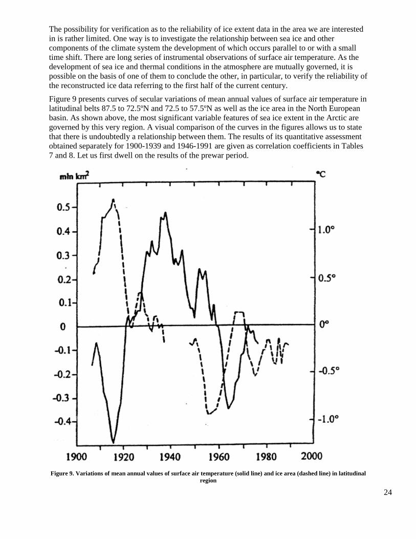
Figure 9 presents curves of secular variations of mean annual values of surface air temperature in latitudinal belts 87.5 to 72.5ºN and 72.5 to 57.5ºN as well as the ice area in the North European basin. As shown above, the most significant variable features of sea ice extent in the Arctic are governed by this very region. A visual comparison of the curves in the figures allows us to state that there is undoubtedly a relationship between them. The results of its quantitative assessment obtained separately for 1900-1939 and 1946-1991 are given as correlation coefficients in Tables 7 and 8. Let us first dwell on the results of the prewar period.

Figure 9. Variations of mean annual values of surface air temperature (solid line) and ice area (dashed line) in latitudinal

region

25

It seems that the first of the indicated periods is characterized by the closet correlation relationship between thermal conditions in the atmosphere and sea ice development, which reaches a maximum at a zero shift in time. It is 0.93 for the latitudinal belt 87.5 to 72.5ºN over 5 year smoothed series. Since high coefficient values are also preserved for the other belts the result should not be considered to be a random. Hence, a conclusion was made that the data of the Danish Meteorological Institute and mean annual sea ice areas reconstructed on their basis for the North European Basin and on the whole in the Atlantic sector of the Arctic present a real picture of the dynamics of marine glaciation in the first half of the 20th century.

Table 7. Correlation coefficients between mean annual ice areas in the North European Basin and surface air temperatures (smoothed by 5 year running periods) synchronously and with a time shift for the period of 1900-1939.

Annual shift -3 -2 -1 -0 +1 +2 +3

87.5-72.5° N -0.64 -0.74 -0.85 -0.93 -0.86 -0.77 -0.68

72.5-57.5° N -0.61 -0.72 -0.82 -0.91 -0.85 -0.79 -0.70

57.5-37.5° N -0.63 -0.62 -0.68 -0.71 -0.62 -0.53 -0.41

Note: a positive shift means temperature lag, a negative one – vice versa.

Table 8.Correlation coefficients between mean annual sea ice area in the North European Basin and surface air temperatures (smoothed by 5 year running periods)

Shift, year -3 -2 -1 -0 +1 +2 +3

87.5-72.5° N -0.91 -0.87 -0.78 -0.62 -0.42 -0.22 -0.05

72.5-57.5° N -0.55 -0.58 -0.60 -0.60 -0.56 -0.50 -0.46

57.5-37.5° N -0.08 -0.10 -0.34 -0.34 -0.56 -0.73 -0.83

It can be concluded from Table 8 that the relationship between thermal conditions in the atmosphere and ice area in the North European Basin was unexpectedly broken in the prewar period. The possible causes of this phenomenon will be discussed when we consider the relationship between the development of sea ice and the physical state of the atmosphere.

26

Relationship of Thermal Conditions in the Atmosphere with the Development of Sea Ice

The first convincing evidence of a close relationship between the Arctic sea ice extent and climate and natural conditions was collected by Toroddsen with regard to Iceland at the beginning of this century. The author has shown by numerous examples that ice appearances off the northern and eastern coast of this island resulted in a sharp air temperature decrease accompanied by an increase of snow fall and fog. Since the vegetation development including fodder grass is governed to a great extent by weather conditions, the appearance and persistence of ice near the shores of Iceland eventually resulted in mass death of cattle and starvation among the population. The situation was aggravated as, due to ice in coastal waters, fishing which always played an important role I the diet of the inhabitants of Iceland [64] reduced dramatically.

The cold summer of 1934 in Japan, which caused a large loss of the rice harvest, took place after a severe winter off the northern coast of Hokkaido Island, according to analysis. This fact led to a theory about the coming summer’s weather conditions dependence on the ice state the previous winter [61]. And examples of this kind are many. The population inhabiting the shores of the ice covered seas knew about the relationship between the ice situation and weather at the coast and, probably used this knowledge in practical activities long before science paid attention to it.

The publication of Toroddsen’s book coincided with the development of the most significant climate fluctuation for the last several centuries. This fluctuation, called at first the warming of the Arctic, was accompanied by a wide spectrum of changes in all spheres of the geographical cover. The analysis of these changes confirmed that the most important moments in the development of the Arctic sea ice cover show close agreement in time and space with variations in the processes in the atmosphere, hydrosphere, cryosphere, and biosphere. Thus, the ice area reduction from the beginning of its systematic observations in the mid 1920’s paralleled the warming development in the atmosphere, heating of the upper ocean layer, rise of its level, reduction of the Arctic and mountain glaciers, and degradation of multi-frozen rocks accompanied by the shift to the north of the boundaries of distribution of marine fish, birds, mammals and vegetation. In the 1940’s these processes reached the limit of development. Gradually, tendencies directly opposite to those which dominated before started to increase and attain a stable character. Simultaneously with the increase of the ice area the cooling in the atmosphere the temperature at sea surface decreased, the rates of the retreat of the glaciers and the rate of the level drop of the World Ocean became slower. In other words, natural processes during this time interval attained a reverse character. In the 1970’s these processes, although not yet demonstrating a pronounced tendency in their development, occurred in accordance with ice cover changes [22, 25].

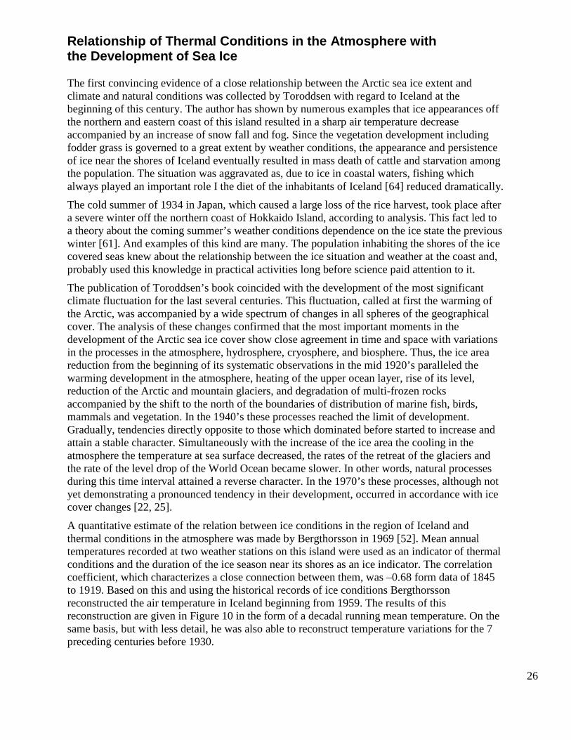
A quantitative estimate of the relation between ice conditions in the region of Iceland and thermal conditions in the atmosphere was made by Bergthorsson in 1969 [52]. Mean annual temperatures recorded at two weather stations on this island were used as an indicator of thermal conditions and the duration of the ice season near its shores as an ice indicator. The correlation coefficient, which characterizes a close connection between them, was –0.68 form data of 1845 to 1919. Based on this and using the historical records of ice conditions Bergthorsson reconstructed the air temperature in Iceland beginning from 1959. The results of this reconstruction are given in Figure 10 in the form of a decadal running mean temperature. On the same basis, but with less detail, he was also able to reconstruct temperature variations for the 7 preceding centuries before 1930.

27

Figure 10. Historical records of ice conditions and

Bergthorsson reconstructed air temperature in Iceland beginning from 1959

The investigation of the relationship between sea ice and thermal conditions in the atmosphere was continued in [26]. We used more generalized indicators of their state and, in particular, ice area in the Arctic Ocean* in July, August and September for 1937-1976 and mean annual air temperatures in the extra-tropical portion of the Northern Hemisphere (87.5 to 17.5° N) and in some latitudinal zones. The correlation coefficient between them turned out to be: for July 0.59 and for September 0.37, when the temperature was taken for the entire extra-equatorial part of

28

the hemisphere. In as much as a close connection between annual data on ice extent in July and mean annual temperature in some latitudinal zones exists, it turned out that the ice extent in the Arctic correlates most closely with the thermal state of the atmosphere of the northernmost zone (85 to 65° N). In this ease the correlation coefficient between these variables was –062. Let us point out a well known feature of this zone: Here the thermal regime change is more and earlier manifested than anywhere else. This feature is more evident during the colder period of the year. In connection with this and particular interest were the correlation coefficient values between total ice extent in each summer month and anomalies of mean half year air temperatures during the cold and warm periods of the year.

*Part of the Arctic Ocean with an area of 10.7 mln km2 Table 9. Correlation coefficients between air temperature anomalies in the latitudinal zone of 85 to 65 N and ice area in the Arctic Ocean

Air temperature anomalies Ice cover extent in

July August September

Cold period of the year -0.66 -0.58 -0.47

Warm period of the year -0.57 -0.64 -0.53

Average over the year -0.60 -0.57 -0.41

As is seen from Table 9, the coefficient values differ a little for cold and warmer periods of the year. But these are small. It is obvious that the polar ice area in summer depends not only on the thermal regime of the summer half of the year. This is confirmed by the coefficients of a multiple linear correlation between the ice cover extent in each of the three summer months and temperature anomalies of both parts of the year. The indicated coefficients constitute –0.71 for the ice cover extent in July and August and –0.58 – in September. And in July, when the Arctic ice area is still close to its annual maximum, it correlated more closely with the anomalies of air temperatures of the colder half a year, while in August and September, i..e. during intensive ice melting with the temperature anomalies of the warm half of the year.

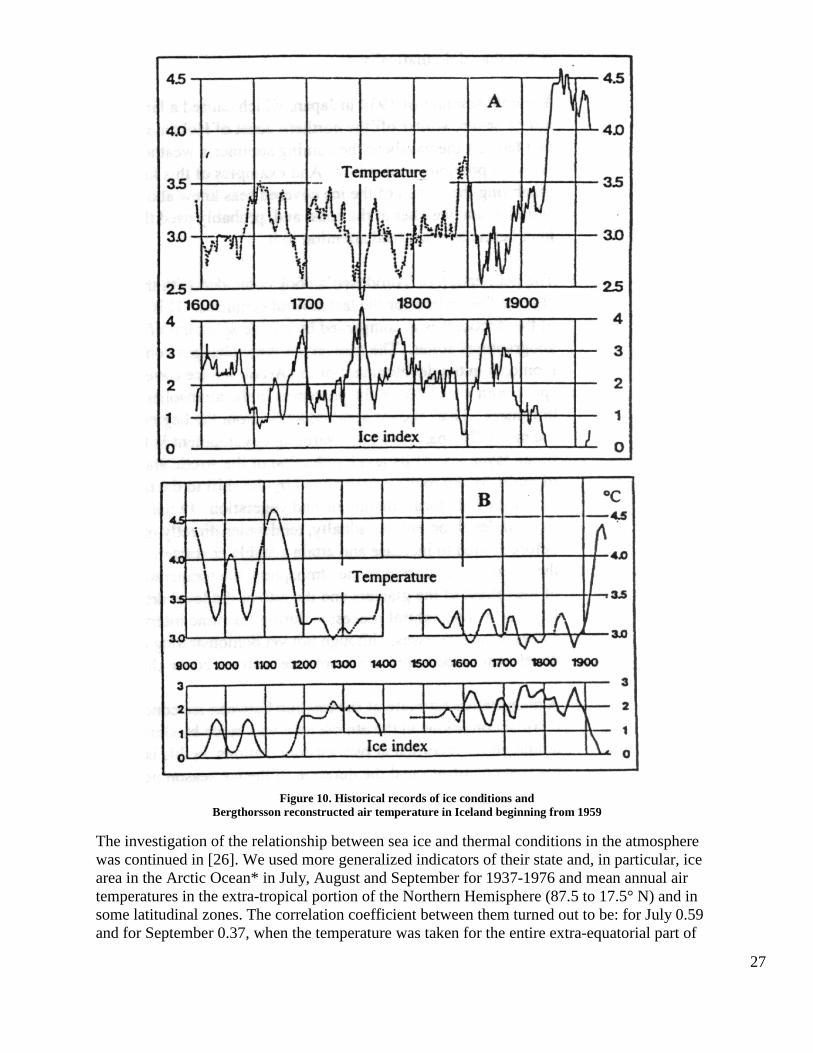
Figure 11 presents multiyear variations of air temperature anomalies in the latitudinal zone 85 to 65° N in the cold and warm parts of the year and ice area in the Arctic Ocean in July and August. We can indicate the presence of an obvious relationship in the variations of temperature anomalies with the ice cover extent changes. The air temperature decrease in the coldest part of the year from five year periods of 1936-1940 to 1965-1969, which was –2.2° C, had a corresponding increase of the ice cover in July of 9.1%. With regard to a mean value over the whole multiyear period and the temperature increase after the period of 19650-1969 by 1.0° C there was corresponding ice area decrease of 5.5%. The amplitude of temperature changes during the warmer half of the year is distinctly less than in the colder one. Thus, in August the temperature drop form 1936-1940 to 1962-1966 was only 0.9° C and the warming of the last period (up to 1972-1976) was expressed by a temperature increase of only 0.3° C. However, the ice area changes in August, corresponding to these changes, were 10.3 and 6.8% from the mean over a multiyear period.

29

Figure 11. Multiyear variations of air temperature

anomalies in the latitudinal zone 85 to 65° N

A more detailed quantitative assessment of the relationship of sea ice with air temperature in the Northern Hemisphere was mad in [3]. The work investigates the dependence between the ice area in the North European Basin, which mainly governs the major features of temporal variability of the ice cover extent for the whole Arctic Ocean, and air temperature at weather stations. The location of most of these stations was selected considering that the ice effect to this basin should be strongest in the so-called zone of the Atlantic influence. The total number of the stations used for the analysis was a little more than 200. The duration of time series for mutual correlation was 30 years in the time interval from 1946 to 1975. The series were not subjected to smoothing.

Figure 12 gives the map of isolines of equal correlations which characterize a close connection between the mean annual ice cover extent to the Northern European Basin and mean annual air temperature north of 40° N. It follows that the area with a negative correlation relationship includes the North Atlantic, part of Western Europe, all European Russia, West Siberia, and the Atlantic sector of the Arctic. The core of the correlation dependence of this sign the coefficient values 0.6-0.7 and a little more is located in the North European Basin and its contours repeat, in a way, sea ice limits in this region.

The geographical location of this core and high coefficient values allow us to assume that the most significant features of the surface temperature regime in the North European Basin are connected in a definite way with the variability in sea ice cover extent here or with the

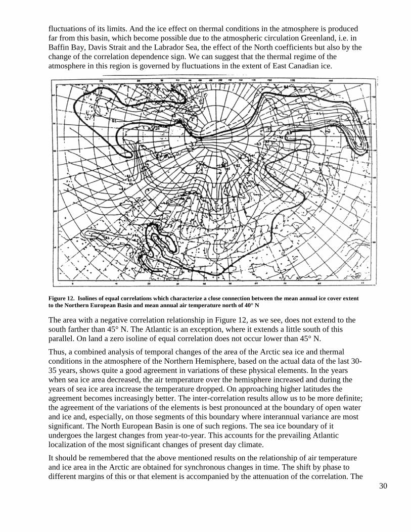
30

fluctuations of its limits. And the ice effect on thermal conditions in the atmosphere is produced far from this basin, which become possible due to the atmospheric circulation Greenland, i.e. in Baffin Bay, Davis Strait and the Labrador Sea, the effect of the North coefficients but also by the change of the correlation dependence sign. We can suggest that the thermal regime of the atmosphere in this region is governed by fluctuations in the extent of East Canadian ice.

Figure 12. Isolines of equal correlations which characterize a close connection between the mean annual ice cover extent to the Northern European Basin and mean annual air temperature north of 40° N

The area with a negative correlation relationship in Figure 12, as we see, does not extend to the south farther than 45° N. The Atlantic is an exception, where it extends a little south of this parallel. On land a zero isoline of equal correlation does not occur lower than 45° N.

Thus, a combined analysis of temporal changes of the area of the Arctic sea ice and thermal conditions in the atmosphere of the Northern Hemisphere, based on the actual data of the last 30-35 years, shows quite a good agreement in variations of these physical elements. In the years when sea ice area decreased, the air temperature over the hemisphere increased and during the years of sea ice area increase the temperature dropped. On approaching higher latitudes the agreement becomes increasingly better. The inter-correlation results allow us to be more definite; the agreement of the variations of the elements is best pronounced at the boundary of open water and ice and, especially, on those segments of this boundary where interannual variance are most significant. The North European Basin is one of such regions. The sea ice boundary of it undergoes the largest changes from year-to-year. This accounts for the prevailing Atlantic localization of the most significant changes of present day climate.

It should be remembered that the above mentioned results on the relationship of air temperature and ice area in the Arctic are obtained for synchronous changes in time. The shift by phase to different margins of this or that element is accompanied by the attenuation of the correlation. The

31

published statements that sea ice development is, probably, delayed as compared with the atmospheric processes should be put aside once and for all. It is impossible to logically explain how the air temperature anomaly of a specific year will affect the ice cover extent in several years or decades.

The recognition of the temporal consistency in air temperature and ice cover extent variations in the Arctic does not give an answer to the central question: what are the cause-effect relationships between them? Are variations in the extent of the Arctic sea ice, as is usually believed, really caused by changes of the thermal state of the atmosphere and not vice versa?

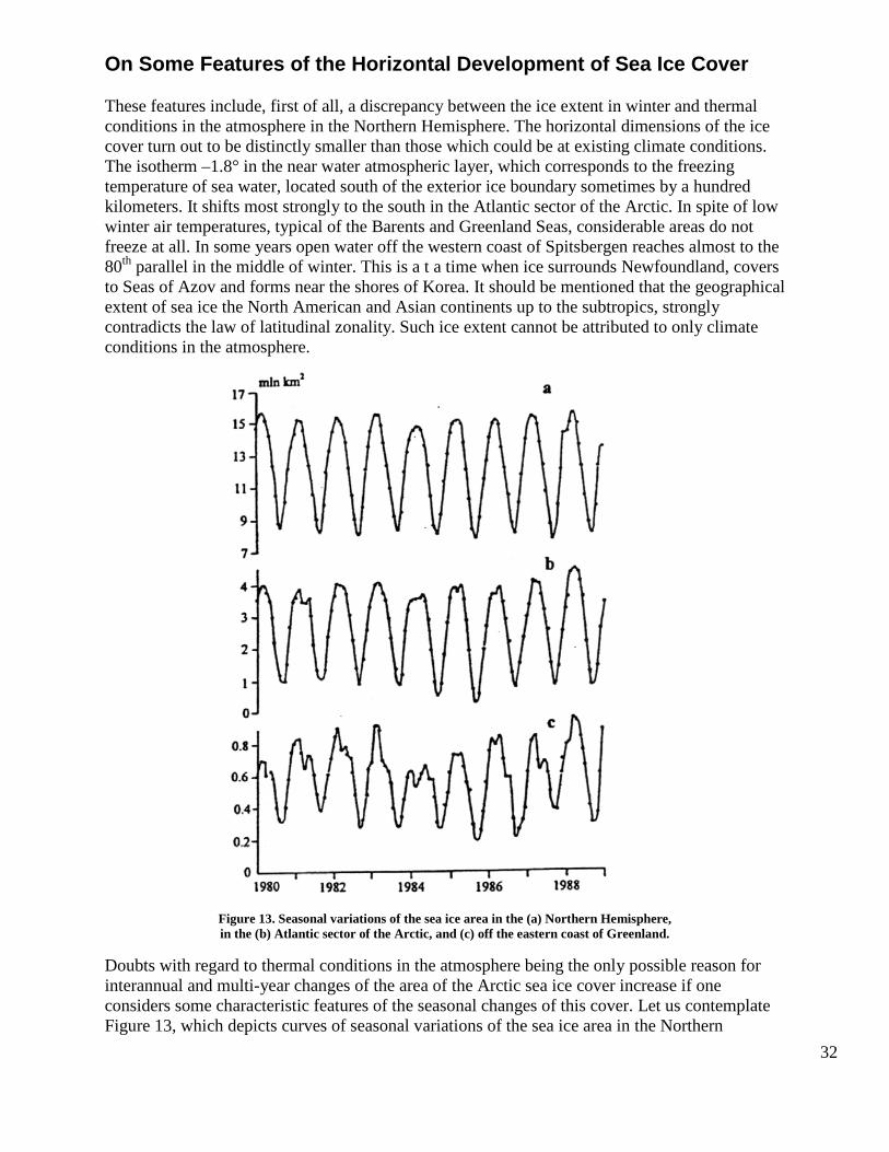
32

On Some Features of the Horizontal Development of Sea Ice Cover

These features include, first of all, a discrepancy between the ice extent in winter and thermal conditions in the atmosphere in the Northern Hemisphere. The horizontal dimensions of the ice cover turn out to be distinctly smaller than those which could be at existing climate conditions. The isotherm –1.8° in the near water atmospheric layer, which corresponds to the freezing temperature of sea water, located south of the exterior ice boundary sometimes by a hundred kilometers. It shifts most strongly to the south in the Atlantic sector of the Arctic. In spite of low winter air temperatures, typical of the Barents and Greenland Seas, considerable areas do not freeze at all. In some years open water off the western coast of Spitsbergen reaches almost to the 80th parallel in the middle of winter. This is a t a time when ice surrounds Newfoundland, covers to Seas of Azov and forms near the shores of Korea. It should be mentioned that the geographical extent of sea ice the North American and Asian continents up to the subtropics, strongly contradicts the law of latitudinal zonality. Such ice extent cannot be attributed to only climate conditions in the atmosphere.

Figure 13. Seasonal variations of the sea ice area in the (a) Northern Hemisphere, in the (b) Atlantic sector of the Arctic, and (c) off the eastern coast of Greenland.

Doubts with regard to thermal conditions in the atmosphere being the only possible reason for interannual and multi-year changes of the area of the Arctic sea ice cover increase if one considers some characteristic features of the seasonal changes of this cover. Let us contemplate Figure 13, which depicts curves of seasonal variations of the sea ice area in the Northern

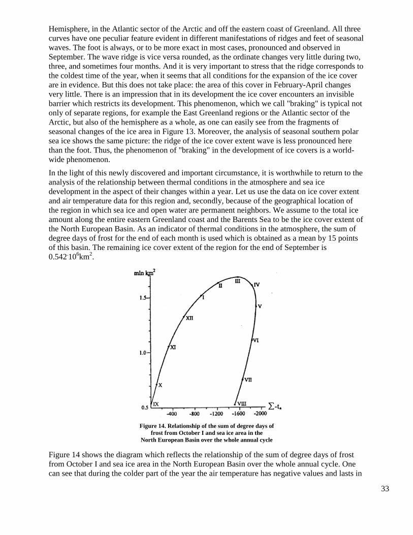
33

Hemisphere, in the Atlantic sector of the Arctic and off the eastern coast of Greenland. All three curves have one peculiar feature evident in different manifestations of ridges and feet of seasonal waves. The foot is always, or to be more exact in most cases, pronounced and observed in September. The wave ridge is vice versa rounded, as the ordinate changes very little during two, three, and sometimes four months. And it is very important to stress that the ridge corresponds to the coldest time of the year, when it seems that all conditions for the expansion of the ice cover are in evidence. But this does not take place: the area of this cover in February-April changes very little. There is an impression that in its development the ice cover encounters an invisible barrier which restricts its development. This phenomenon, which we call "braking" is typical not only of separate regions, for example the East Greenland regions or the Atlantic sector of the Arctic, but also of the hemisphere as a whole, as one can easily see from the fragments of seasonal changes of the ice area in Figure 13. Moreover, the analysis of seasonal southern polar sea ice shows the same picture: the ridge of the ice cover extent wave is less pronounced here than the foot. Thus, the phenomenon of "braking" in the development of ice covers is a world-wide phenomenon.

In the light of this newly discovered and important circumstance, it is worthwhile to return to the analysis of the relationship between thermal conditions in the atmosphere and sea ice development in the aspect of their changes within a year. Let us use the data on ice cover extent and air temperature data for this region and, secondly, because of the geographical location of the region in which sea ice and open water are permanent neighbors. We assume to the total ice amount along the entire eastern Greenland coast and the Barents Sea to be the ice cover extent of the North European Basin. As an indicator of thermal conditions in the atmosphere, the sum of degree days of frost for the end of each month is used which is obtained as a mean by 15 points of this basin. The remaining ice cover extent of the region for the end of September is 0.542.106km2.

Figure 14. Relationship of the sum of degree days of

frost from October I and sea ice area in the North European Basin over the whole annual cycle

Figure 14 shows the diagram which reflects the relationship of the sum of degree days of frost from October I and sea ice area in the North European Basin over the whole annual cycle. One can see that during the colder part of the year the air temperature has negative values and lasts in

34

this basin from the end of September to the end of May. During the period June-September the air temperatures here are positive. In accordance with this the development of the ice cover is divided into two phases quite different in their duration: expansion, which lasts 8 months and reduction which is half as long. The curve is open: the sum of negative air temperatures prevails quite distinctly over the sum of positive temperatures. The heat deficit, which forms in such a way in the basin, is compensated due to the ocean heat.

The relationship between the sea ice area and the sum of degree days of frost is characterized by the following features. It can be assumed to be linear only at the first stage of the ice cover expansion, which lasts from the end of September to mid-January in the best case. In the subsequent 4.5-5 months, i.e. up to the end of the expansion phase, there is a progressive braking of the ice area increase. Thus, if during December at degree days of frost -297, the ice area growth was 0.272-106 km2, then in January at the sum of degree days -325 it was 0. 195, in February at the sum of degree days -3 10 the growth decreased to 0.114, and renewed only with the phase of the ice cover reduction, i.e. from early June and lasts till the end of September.

35

Factors of Ice Formation and Melting

Let us consider in more detail the factors which govern ice formation and melting in the sea and account for the "strange" development of ice cover within a year. An impressive picture of the development of sea ice cover within time frames of glacial, interglacial, seasonal, and multiyear fluctuations is associated with the processes of formation and melting. These processes are, in turn, governed by a number of physical factors. Without a clear understanding of these one cannot understand the connection between the conditions in the atmosphere and sea ice. Let us look at them, beginning with the ice formation process. We shall use the dependent relationship found between the date of the onset of ice formation and the hydro-meteorological factors governing it [21].

and

Where τ = time in days from the initial moment the water reaches freezing temperature; tw = initial water temperature in degrees of the active layer; tc = water freezing temperature in degrees of a given salinity; h = initial thickness of the active layer in meters; ∆S = horizontal salinity gradient % per 100 km by the direction of the prevailing water mass transfer; µ= vertical salinity gradient in the halocline, degrees per meter; v = wind speed, meters per second; ta air temperature degrees averaged over the period; tao= degrees air temperature at the initial moment; ta1 = degrees air temperature at the moment ice formation begins; Ro and R1= radiation balance at the beginning and end of the time frame, calculated in cm2 per day.

The numerator of this formula represents the heat content of the convection layer, and the denominator represents the loss intensity as a result of radiative and turbulent heat exchange and moisture turnover with the atmosphere. Based on this dependence we conclude that ice formation is governed not only by meteorological factors regulating the cooling of the upper ocean layer but also by temperature and thickness of the latter. This important finding should be remembered when discussing the effect of climate changes on sea ice extent. It is not difficult to imagine the conditions at which the ocean effect and, in particular, its thermal state can be decisive for its freezing or, vice versa, the preservation of open water.

Of course, this effect is limited only to the colder part of the year when vertical stability of the layers in the ocean is attenuated and heat fluxes from the depths to the surface are enhanced. With the beginning of melting and the outflow of melt waters, there forms under the ice a blocking layer which attenuates the heat input from below up to values which can be neglected. The dominate role during the period of ice melting is played by radiation and meteorological factors. This includes air temperature which is expressed, for example, in the formula for the determination of the ice melt value [20].

36

where: ∆H= ice thickness, melted from above for N days; Ri = radiation balance of the underlying surface for i days; pc and ps density of snow and ice; vi = relative air humidity at the level of the meteorological both during i days; Ti = temperature at the level of the meteorological booth during i days; 4j = 0.4 + 0.48 n; and n = wind speed measured at the weathervane height.

Thus, we can say that the role of atmospheric factors in the sea ice extent does not remain constant during the year. While inter-annual and multi-year ice area summer variations can be entirely attributed to the variability of atmospheric factors, this cannot be done with regard to winter. Ice area fluctuations during the colder period of the year, as it has been mentioned, are not necessarily governed by meteorological factors alone. They can also be induced by the changes in the heat content and thickness of the layer participating in the energy exchange with the atmosphere. The phenomenon of braking, which was mentioned in the previous section, is most probably related to the effect of the ocean on sea ice extent during the colder period of the year.

37

Conditions in the Ocean and Sea Ice Development

Ice formation begins when the heat flux to the atmosphere from the surface of the water reservoir exceeds its income from deep water layers. The heat deficit which forms is compensated for by the crystallization heat at the water transition from the liquid state to the solid one. Obviously, where annual ocean heat losses exceed the amount of solar energy to it, in winter, the necessary conditions are created for sea ice formation. The so-called areas of the energy outflow meet these conditions. They cover not only Polar Regions, but also significant zones of temperate latitudes in both hemispheres. Figure 16 [editor’s note: missing graphic] shows the heat budget at the surface of the world's ocean from the equator to the poles. The latitudinal belt between 30' N and 20' S is the domain of energy accumulation: the amount of absorbed heat here exceeds the losses due to evaporation and turbulent heat exchange. The regions north and south of the boundaries of this belt are the regions of the energy outflow: the amount of the incoming solar energy is here less than its loss. In the absence of the horizontal heat transfer from low to higher latitudes, there would be heating of the equatorial belt and cooling of extra-equatorial latitudes.

However, the conditions for sea ice formation present in the energy outflow domains are not fulfilled in all cases. Suffice it to say that at least the North European Basin which is located deep in the area of the energy discharge does not freeze over much of its territory. The reason for this is that in the energy exchange with the atmosphere in addition to the heat accumulated annually in this basin the advective heat, centered in the ocean depths and continuously supplemented by the currents, participates (Figure 15). When this heat has direct access to the ocean surface, ice is not formed. When this condition is not fulfilled and the outflow of advective heat is not possible or attenuated to such extent that it cannot fully compensate for the heat outflow to the atmosphere, ice formation becomes inevitable. In other words, the existence of the ice or ice free regimes in the energy outflow domain depends on the extent of the advective heat participation in the energy exchange with the atmosphere. The role played by advective heat in the energy outflow domain in the maintenance of the ice free regime makes it necessary to exclude the factors regulating its transfer to the ocean surface. This is because the currents which transport the heat in the direction of the poles lie in the depths and do, not have direct contact with the atmosphere.

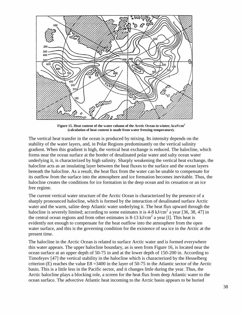
38

Figure 15. Heat content of the water column of the Arctic Ocean in winter, kcaVcm2

(calculation of heat content is made from water freezing temperature).

The vertical heat transfer in the ocean is produced by mixing. Its intensity depends on the stability of the water layers, and, in Polar Regions predominantly on the vertical salinity gradient. When this gradient is high, the vertical heat exchange is reduced. The halocline, which forms near the ocean surface at the border of desalinated polar water and salty ocean water underlying it, is characterized by high salinity. Sharply weakening the vertical heat exchange, the halocline acts as an insulating layer between the heat fluxes to the surface and the ocean layers beneath the halocline. As a result, the heat flux from the water can be unable to compensate for its outflow from the surface into the atmosphere and ice formation becomes inevitable. Thus, the halocline creates the conditions for ice formation in the deep ocean and its cessation or an ice free regime.

The current vertical water structure of the Arctic Ocean is characterized by the presence of a sharply pronounced halocline, which is formed by the interaction of desalinated surface Arctic water and the warm, saline deep Atlantic water underlying it. The heat flux upward through the halocline is severely limited; according to some estimates it is 4-8 kJ/cm2 a year [36, 38, 47] in the central ocean regions and from other estimates is 8-13 kJ/cm2 a year [l]. This heat is evidently not enough to compensate for the heat outflow into the atmosphere from the open water surface, and this is the governing condition for the existence of sea ice in the Arctic at the present time.

The halocline in the Arctic Ocean is related to surface Arctic water and is formed everywhere this water appears. The upper halocline boundary, as is seen from Figure 16, is located near the ocean surface at an upper depth of 50-75 in and at the lower depth of 150-200 in. According to Timofeyev [47] the vertical stability in the halocline which is characterized by the Hesselberg criterion (E) reaches the value E8 =3400 in the layer of 50-75 in the Atlantic sector of the Arctic basin. This is a little less in the Pacific sector, and it changes little during the year. Thus, the Arctic halocline plays a blocking role, a screen for the heat flux from deep Atlantic water to the ocean surface. The advective Atlantic heat incoming to the Arctic basin appears to be buried

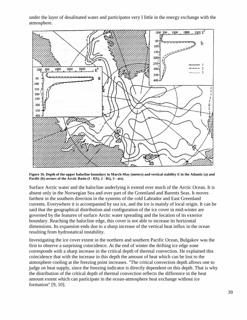
39

under the layer of desalinated water and participates very I little in the energy exchange with the atmosphere.

Figure 16. Depth of the upper halocline boundary in March-May (meters) and vertical stability E in the Atlantic (a) and Pacific (b) sectors of the Arctic Basin (I - f(S); 2 - Rt), 3 - ats).

Surface Arctic water and the halocline underlying it extend over much of the Arctic Ocean. It is absent only in the Norwegian Sea and over part of the Greenland and Barents Seas. It moves farthest in the southern direction in the systems of the cold Labrador and East Greenland currents. Everywhere it is accompanied by sea ice, and the ice is mainly of local origin. It can be said that the geographical distribution and configuration of the ice cover in mid-winter are governed by the features of surface Arctic water spreading and the location of its exterior boundary. Reaching the halocline edge, this cover is not able to increase its horizontal dimensions. Its expansion ends due to a sharp increase of the vertical heat influx in the ocean resulting from hydrostatical instability.

Investigating the ice cover extent in the northern and southern Pacific Ocean, Bulgakov was the first to observe a surprising coincidence. At the end of winter the drifting ice edge zone corresponds with a sharp increase in the critical depth of thermal convection. He explained this coincidence that with the increase in this depth the amount of heat which can be lost to the atmosphere cooling at the freezing point increases. "The critical convection depth allows one to judge on heat supply, since the freezing indicator is directly dependent on this depth. That is why the distribution of the critical depth of thermal convection reflects the difference in the heat amount extent which can participate in the ocean-atmosphere heat exchange without ice formation" [9, 10].

40

A similar picture is typical of the Southern Ocean too. Treshnikov, Shpaikher, and Gindysh noticed a close correlation between the isoline of the 100 m convection depth and the maximum boundary of the Antarctic sea ice [48].

The interdependence of the halocline and sea ice allows us to also understand the reason for violation of the law of latitudinal zonality in the sea ice extent in the Northern hemisphere and explains the "braking" phenomenon. It is in the features of the geographical distribution of the halocline which, like a gigantic screen, blocks the heat flux from the depths to the ocean surface and, thus, creates the necessary conditions for ice formation. These conditions are fulfilled when the air temperature in winter drops below the sea water freezing temperature for quite a long time. As a result, by the end of winter and in some regions even earlier, the ice cover extends over the whole domain of the polar halocline. ne sea ice edge becomes stable at its exterior boundary and even the persisting cold is not able to shift it. These conditions are most evident in the North European basin in the contact zone of cold and warm currents and desalinated and salty waters. The ice edge in this basin reaches the halocline boundary, the limit of its development in the horizontal direction in February.

A natural analogue of the phenomenon which characterized the sea ice dependence on the halocline is very interesting. We mean the formation of ice at positive water and air temperatures which has been publicized many times. Among the investigators were Scorsby, Nordenskjold, Amold-Alyabyev, and Zubov. We observed this phenomenon in August of 1958 in the vicinity of the New Siberian Islands. When the sun was low on the horizon in open water in clear and windless weather we observed in the fractures dim dark patches of newly formed ice, to be more exact an ice film. These patches, as a rule, were isolated from each other by narrow areas of open water. Small in size - not more than 1.5 m in diameter and very thin - they were destroyed by a weak ship wave and disappeared rapidly. The water temperature measured at the surface at this time was equal to +0.9 and the air temperature was +0.3'C. As it has been found, the formation of ice patches on sea surface at positive water and air temperatures becomes possible during the combination of some favorable circumstances. One of them is a thin film of fresh water on the sea surface. In the Arctic Seas such a film can form during windless weather in fractures due to a slow spreading of fresh water from melting ice. In the absence of wind and currents and at a temperature close to the freezing point, this fresh water does not mix with sea water, being stratified in a stable way. At low angles over the horizon the amount of incoming solar energy to the sea surface is small. Under an open sky the heat emission can prevail over its income from the Sun. The fresh water film is cooled up to the freezing temperature and patches of very thin ice appear on the surface. However, small amounts of mixing can induce warm water up to the surface and this is enough to make the formed ice disappear at once.

Surface Arctic water, which vertically occupies less than 2% of the ocean water column and which is under constant cooling during the long polar night, is essentially the same thin film of light water which results in ice formation at a positive temperature. Thus, the resulting conclusion to the questions set forth in this section is that the cause-effect relationship between sea ice and thermal conditions in the atmosphere are of a more complicated character than is usually believed. An understanding that sea ice only responds to climate changes, i.e. being a result of the change of the latter, is only partly true. The ice area changes in summer and fall can be considered to be climatically governed, mainly when radiation and meteorological factors have a decisive importance in the changes of the ice cover state. For example, in the North European basin this period is 7-7.5 months, from early June to early mid-January. During the rest of the year the ice cover development is mainly restricted by the conditions in the ocean, depending on the development of the Arctic halocline.

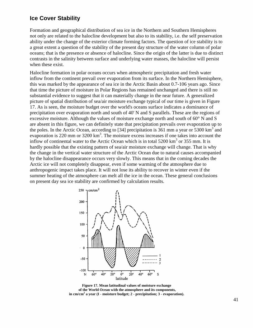
41

Ice Cover Stability

Formation and geographical distribution of sea ice in the Northern and Southern Hemispheres not only are related to the halocline development but also to its stability, i.e. the self preservation ability under the change of the exterior climate forming factors. The question of ice stability is to a great extent a question of the stability of the present day structure of the water column of polar oceans; that is the presence or absence of halocline. Since the origin of the latter is due to distinct contrasts in the salinity between surface and underlying water masses, the halocline will persist when these exist.

Halocline formation in polar oceans occurs when atmospheric precipitation and fresh water inflow from the continent prevail over evaporation from its surface. In the Northern Hemisphere, this was marked by the appearance of sea ice in the Arctic Basin about 0.7-106 years ago. Since that time the picture of moisture in Polar Regions has remained unchanged and there is still no substantial evidence to suggest that it can materially change in the near future. A generalized picture of spatial distribution of sea/air moisture exchange typical of our time is given in Figure 17. As is seen, the moisture budget over the world's oceans surface indicates a dominance of precipitation over evaporation north and south of 40' N and S parallels. These are the regions of excessive moisture. Although the values of moisture exchange north and south of 60° N and S are absent in this figure, we can definitely state that precipitation prevails over evaporation up to the poles. In the Arctic Ocean, according to [34] precipitation is 361 mm a year or 5300 km3 and evaporation is 220 mm or 3200 km3. The moisture excess increases if one takes into account the inflow of continental water to the Arctic Ocean which is in total 5200 km3 or 355 mm. It is hardly possible that the existing pattern of sea/air moisture exchange will change. That is why the change in the vertical water structure of the Arctic Ocean due to natural causes accompanied by the halocline disappearance occurs very slowly. This means that in the coming decades the Arctic ice will not completely disappear, even if some warming of the atmosphere due to anthropogenic impact takes place. It will not lose its ability to recover in winter even if the summer heating of the atmosphere can melt all the ice in the ocean. These general conclusions on present day sea ice stability are confirmed by calculation results.

Figure 17. Mean latitudinal values of moisture exchange

of the World Ocean with the atmosphere and its components, in cm/cm2 a year (I - moisture budget; 2 - precipitation; 3 - evaporation).

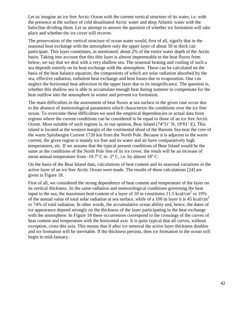
42

Let us imagine an ice free Arctic Ocean with the current vertical structure of its water, i.e. with the presence at the surface of cold desalinated Arctic water and deep Atlantic water with the halocline dividing them. Let us attempt to answer the question of whether ice formation will take place and whether the ice cover will recover.

The preservation of the vertical structure of ocean water would, first of all, signify that in the seasonal heat exchange with the atmosphere only the upper layer of about 50 m thick can participate. This layer constitutes, as mentioned, about 2% of the entire water depth of the Arctic basin. Taking into account that this thin layer is almost impermeable to the heat fluxes from below, we say that we deal with a very shallow sea. The seasonal heating and cooling of such a sea depends entirely on its heat exchange with the atmosphere. These can be calculated on the basis of the heat balance equation, the components of which are solar radiation absorbed by the sea, effective radiation, turbulent heat exchange and heat losses due to evaporation. One can neglect the horizontal heat advection in the upper layer due to its insignificance. The question is, whether this shallow sea is able to accumulate enough heat during summer to compensate for the heat outflow into the atmosphere in winter and prevent ice formation.

The main difficulties in the assessment of heat fluxes at sea surface in the given case occur due to the absence of meteorological parameters which characterize the conditions over the ice free ocean. To overcome these difficulties we used the empirical dependencies or actual data from regions where the current conditions can be considered to be equal to those of an ice free Arctic Ocean. Most suitable of such regions is, in our opinion, Bear Island (74º31’ N, 19º01’ E). This island is located at the western margin of the continental shoal of the Barents Sea near the core of the warm Spitsbergen Current 1720 km from the North Pole. Because it is adjacent to the warm current, the given region is mainly ice free and its water and air have comparatively high temperatures, etc. If we assume that the typical present conditions of Bear Island would be the same as the conditions of the North Pole free of its ice cover, the result will be an increase of mean annual temperature from -19.7º C to -2º C, i.e. by almost 18º C.

On the basis of the Bear Island data, calculations of heat content and its seasonal variations in the active layer of an ice free Arctic Ocean were made. The results of these calculations [24] are given in Figure 18.

First of all, we considered the strong dependence of heat content and temperature of the layer on its vertical thickness. At the same radiation and meteorological conditions governing the heat input to the sea, the maximum heat content of a layer of 10 in constitutes 11.5 kcal/cm2 or 19% of the annual value of total solar radiation at sea surface, while of a 100 m layer it is 45 kcal/cm2 or 74% of total radiation. In other words, the accumulative ocean ability and, hence, the dates of ice appearance depend strongly on the thickness of the layer participating in the heat exchange with the atmosphere. In Figure 18 these occurrences correspond to the crossings of the curves of heat content and temperature with the horizontal axis. It is quite typical that all curves, without exception, cross this axis. This means that if after ice removal the active layer thickness doubles and ice formation will be inevitable. If the thickness persists, then ice formation in the ocean will begin in mid-January.

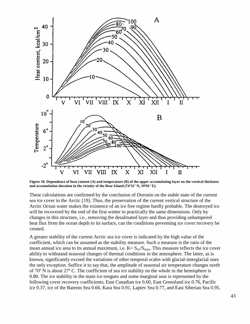
43

Figure 18. Dependence of heat content (A) and temperature (B) of the upper accumulating layer on the vertical thickness and accumulation duration in the vicinity of the Bear Island (74º31’ N, 19º01’ E).

These calculations are confirmed by the conclusion of Doronin on the stable state of the current sea ice cover in the Arctic [19]. Thus, the preservation of the current vertical structure of the Arctic Ocean water makes the existence of an ice free regime hardly probable. The destroyed ice will be recovered by the end of the first winter in practically the same dimensions. Only by changes in this structure, i.e., removing the desalinated layer and thus providing unhampered heat flux from the ocean depth to its surface, can the conditions preventing ice cover recovery be created.

A greater stability of the current Arctic sea ice cover is indicated by the high value of the coefficient, which can be assumed as the stability measure. Such a measure is the ratio of the mean annual ice area to its annual maximum, i.e. K= Sav/Smax. This measure reflects the ice cover ability to withstand seasonal changes of thermal conditions in the atmosphere. The latter, as is known, significantly exceed the variations of other temporal scales with glacial-interglacial ones the only exception. Suffice it to say that, the amplitude of seasonal air temperature changes north of 70º N is about 27º C. The coefficient of sea ice stability on the whole in the hemisphere is 0.80. The ice stability in the main ice tongues and some marginal seas is represented by the following cover recovery coefficients; East Canadian ice 0.60, East Greenland ice 0.76, Pacific ice 0.37, ice of the Barents Sea 0.66, Kara Sea 0.91, Laptev Sea 0.77, and East Siberian Sea 0.95.

44

A stable state of sea ice in the Arctic is an important factor to climate conditions in the Northern Hemisphere. Sharp variations of these conditions, inducing a cardinal change in the environment, are simply impossible during short time intervals. This is confirmed by distinct but rather limited climate changes over the historical period. Maybe the most convincing evidence of the Arctic sea ice stability is its preservation during the last 0.7 ml. years despite vast glacial- interglacial fluctuations. The surface air temperature in the Arctic during the interglacial periods was higher by several degrees than present day temperatures.

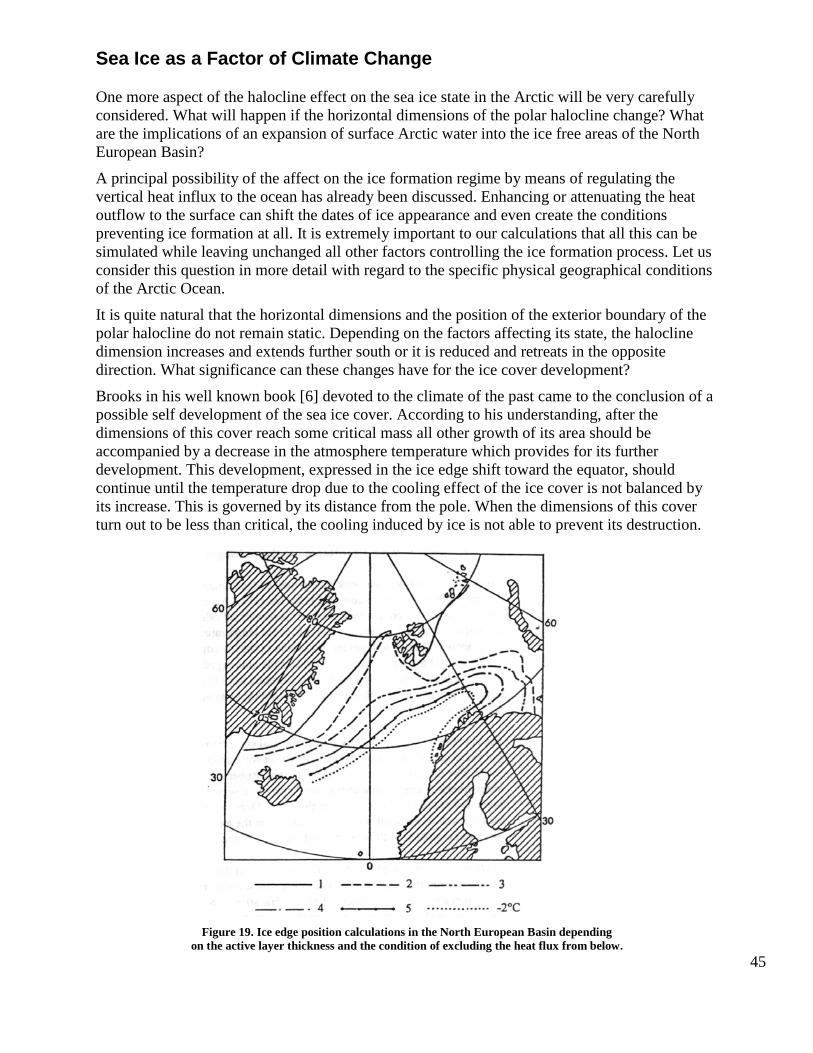
45

Sea Ice as a Factor of Climate Change

One more aspect of the halocline effect on the sea ice state in the Arctic will be very carefully considered. What will happen if the horizontal dimensions of the polar halocline change? What are the implications of an expansion of surface Arctic water into the ice free areas of the North European Basin?

A principal possibility of the affect on the ice formation regime by means of regulating the vertical heat influx to the ocean has already been discussed. Enhancing or attenuating the heat outflow to the surface can shift the dates of ice appearance and even create the conditions preventing ice formation at all. It is extremely important to our calculations that all this can be simulated while leaving unchanged all other factors controlling the ice formation process. Let us consider this question in more detail with regard to the specific physical geographical conditions of the Arctic Ocean.

It is quite natural that the horizontal dimensions and the position of the exterior boundary of the polar halocline do not remain static. Depending on the factors affecting its state, the halocline dimension increases and extends further south or it is reduced and retreats in the opposite direction. What significance can these changes have for the ice cover development?

Brooks in his well known book [6] devoted to the climate of the past came to the conclusion of a possible self development of the sea ice cover. According to his understanding, after the dimensions of this cover reach some critical mass all other growth of its area should be accompanied by a decrease in the atmosphere temperature which provides for its further development. This development, expressed in the ice edge shift toward the equator, should continue until the temperature drop due to the cooling effect of the ice cover is not balanced by its increase. This is governed by its distance from the pole. When the dimensions of this cover turn out to be less than critical, the cooling induced by ice is not able to prevent its destruction.

Figure 19. Ice edge position calculations in the North European Basin depending

on the active layer thickness and the condition of excluding the heat flux from below.

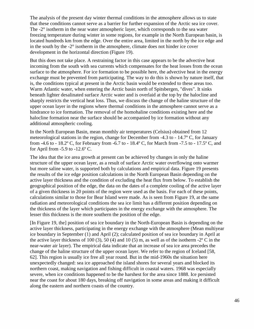
46

The analysis of the present day winter thermal conditions in the atmosphere allows us to state that these conditions cannot serve as a barrier for further expansion of the Arctic sea ice cover. The -2° isotherm in the near water atmospheric layer, which corresponds to the sea water freezing temperature during winter in some regions, for example in the North European basin, is located hundreds km from the edge. Over the entire area, limited in the north by the ice edge and in the south by the -2° isotherm in the atmosphere, climate does not hinder ice cover development in the horizontal direction (Figure 19).

But this does not take place. A restraining factor in this case appears to be the advective heat incoming from the south with sea currents which compensates for the heat losses from the ocean surface to the atmosphere. For ice formation to be possible here, the advective heat in the energy exchange must be prevented from participating. The way to do this is shown by nature itself, that is, the conditions typical at present in the Arctic basin would be extended to these areas too. Warm Atlantic water, when entering the Arctic basin north of Spitsbergen, "dives". It sinks beneath lighter desalinated surface Arctic water and is overlaid at the top by the halocline and sharply restricts the vertical heat loss. Thus, we discuss the change of the haline structure of the upper ocean layer in the regions where thermal conditions in the atmosphere cannot serve as a hindrance to ice formation. The removal of the homohaline conditions existing here and the halocline formation near the surface should be accompanied by ice formation without any additional atmospheric cooling.

In the North European Basin, mean monthly air temperatures (Celsius) obtained from 12 meteorological stations in the region, change for December from -4.3 to - 14.7º C, for January from -4.6 to - 18.2º C, for February from -6.7 to - 18.4º C, for March from -7.5 to - 17.5º C, and for April from -5.9 to -12.6º C.

The idea that the ice area growth at present can be achieved by changes in only the haline structure of the upper ocean layer, as a result of surface Arctic water overflowing onto warmer but more saline water, is supported both by calculations and empirical data. Figure 19 presents the results of the ice edge position calculations in the North European Basin depending on the active layer thickness and the condition of excluding the heat flux from below. To establish the geographical position of the edge, the data on the dates of a complete cooling of the active layer of a given thickness in 20 points of the region were used as the basis. For each of these points, calculations similar to those for Bear Island were made. As is seen from Figure 19, at the same radiation and meteorological conditions the sea ice limit has a different position depending on the thickness of the layer which participates in the energy exchange with the atmosphere. The lesser this thickness is the more southern the position of the edge.

[In Figure 19, the] position of sea ice boundary in the North-European Basin is depending on the active layer thickness, participating in the energy exchange with the atmosphere (Mean multiyear ice boundary in September (1) and April (2); calculated position of sea ice boundary in April at the active layer thickness of 100 (3), 50 (4) and 10 (5) m, as well as of the isotherm -2º C in the near-water air layer). The empirical data indicate that an increase of sea ice area precedes the change of the haline structure of the upper ocean layer. We refer to the region of Iceland [58, 62]. This region is usually ice free all year round. But in the mid-1960s the situation here unexpectedly changed: sea ice approached the island shores for several years and blocked its northern coast, making navigation and fishing difficult in coastal waters. 1968 was especially severe, when ice conditions happened to be the harshest for the area since 1888. Ice persisted near the coast for about 180 days, breaking off navigation in some areas and making it difficult along the eastern and northern coasts of the country.

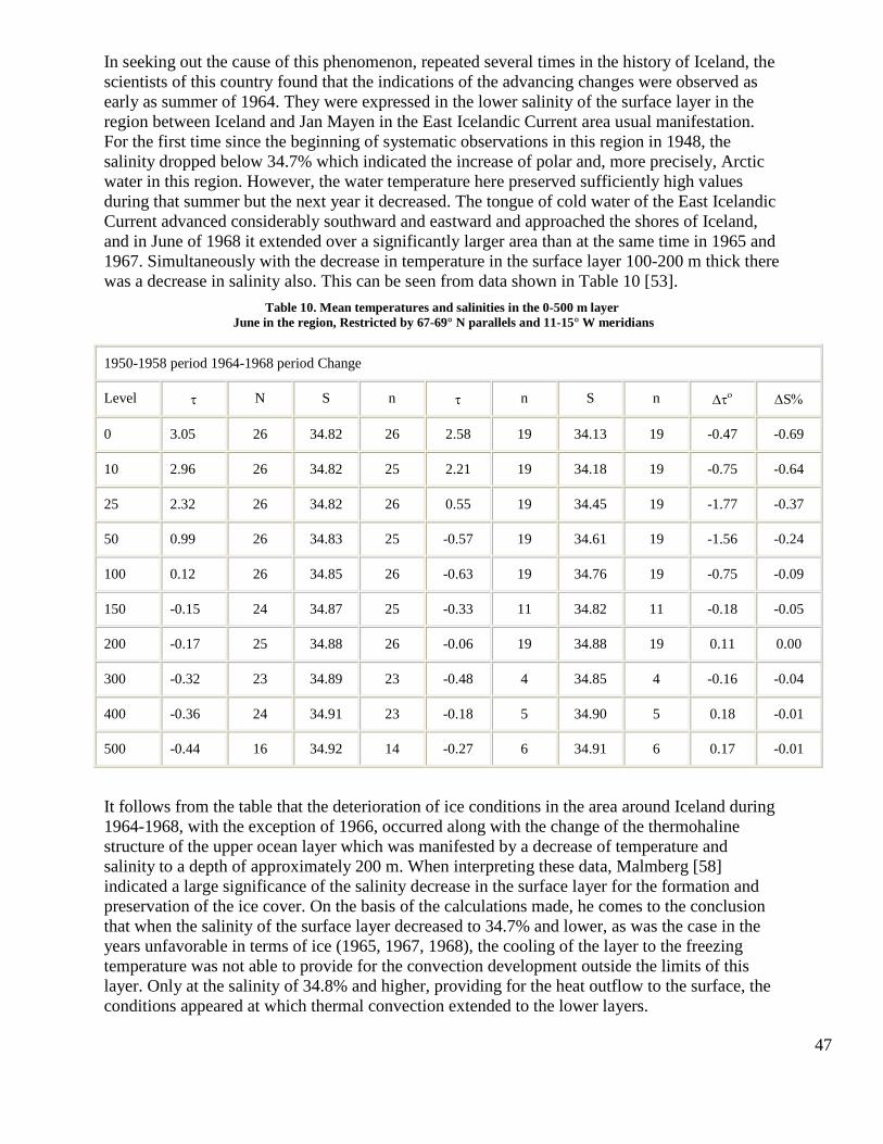
47

In seeking out the cause of this phenomenon, repeated several times in the history of Iceland, the scientists of this country found that the indications of the advancing changes were observed as early as summer of 1964. They were expressed in the lower salinity of the surface layer in the region between Iceland and Jan Mayen in the East Icelandic Current area usual manifestation. For the first time since the beginning of systematic observations in this region in 1948, the salinity dropped below 34.7% which indicated the increase of polar and, more precisely, Arctic water in this region. However, the water temperature here preserved sufficiently high values during that summer but the next year it decreased. The tongue of cold water of the East Icelandic Current advanced considerably southward and eastward and approached the shores of Iceland, and in June of 1968 it extended over a significantly larger area than at the same time in 1965 and 1967. Simultaneously with the decrease in temperature in the surface layer 100-200 m thick there was a decrease in salinity also. This can be seen from data shown in Table 10 [53].

Table 10. Mean temperatures and salinities in the 0-500 m layer June in the region, Restricted by 67-69° N parallels and 11-15° W meridians

1950-1958 period 1964-1968 period Change

Level τ N S n τ n S n ∆το ∆S%

0 3.05 26 34.82 26 2.58 19 34.13 19 -0.47 -0.69

10 2.96 26 34.82 25 2.21 19 34.18 19 -0.75 -0.64

25 2.32 26 34.82 26 0.55 19 34.45 19 -1.77 -0.37

50 0.99 26 34.83 25 -0.57 19 34.61 19 -1.56 -0.24

100 0.12 26 34.85 26 -0.63 19 34.76 19 -0.75 -0.09

150 -0.15 24 34.87 25 -0.33 11 34.82 11 -0.18 -0.05

200 -0.17 25 34.88 26 -0.06 19 34.88 19 0.11 0.00

300 -0.32 23 34.89 23 -0.48 4 34.85 4 -0.16 -0.04

400 -0.36 24 34.91 23 -0.18 5 34.90 5 0.18 -0.01

500 -0.44 16 34.92 14 -0.27 6 34.91 6 0.17 -0.01

It follows from the table that the deterioration of ice conditions in the area around Iceland during 1964-1968, with the exception of 1966, occurred along with the change of the thermohaline structure of the upper ocean layer which was manifested by a decrease of temperature and salinity to a depth of approximately 200 m. When interpreting these data, Malmberg [58] indicated a large significance of the salinity decrease in the surface layer for the formation and preservation of the ice cover. On the basis of the calculations made, he comes to the conclusion that when the salinity of the surface layer decreased to 34.7% and lower, as was the case in the years unfavorable in terms of ice (1965, 1967, 1968), the cooling of the layer to the freezing temperature was not able to provide for the convection development outside the limits of this layer. Only at the salinity of 34.8% and higher, providing for the heat outflow to the surface, the conditions appeared at which thermal convection extended to the lower layers.

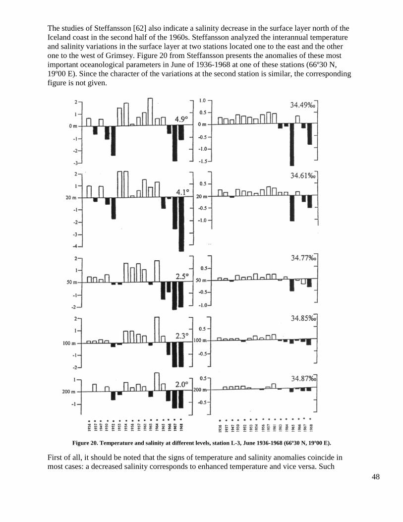
48

The studies of Steffansson [62] also indicate a salinity decrease in the surface layer north of the Iceland coast in the second half of the 1960s. Steffansson analyzed the interannual temperature and salinity variations in the surface layer at two stations located one to the east and the other one to the west of Grimsey. Figure 20 from Steffansson presents the anomalies of these most important oceanological parameters in June of 1936-1968 at one of these stations (66º30 N, 19º00 E). Since the character of the variations at the second station is similar, the corresponding figure is not given.

Figure 20. Temperature and salinity at different levels, station L-3, June 1936-1968 (66º30 N, 19º00 E).

First of all, it should be noted that the signs of temperature and salinity anomalies coincide in most cases: a decreased salinity corresponds to enhanced temperature and vice versa. Such

49

similarity in the change of these parameters is impossible to explain from the point of view of the governing role of thermal conditions in the atmosphere with regard to the ocean, as the air temperature increase and decrease can result only in the change of the thermal state of sea surface layer not its salinity.

The temperature and salinity changes mainly occur in the upper 200 in layer. At the lower boundary of this layer the salinity deviations from its mean value for 1936-1969 did not exceed 0.2% in both directions. This fact indicates that the most significant change of the thermohaline structure takes place in the upper ocean layer.

The deterioration of ice conditions in the area of Iceland coincides with the desalination of the sea surface layer and its temperature decrease. This result is fully consistent with the conclusions of Malmberg about the existence of a close relationship between ice conditions in Icelandic waters in spring of 1965, 1967 and 1968 and oceanographic conditions in the upper layer. It appears there is no reason not to agree with Malmberg on the existence of a close relationship between ice conditions and oceanographic conditions in the upper layer in Icelandic waters in spring of 1965, 1967 and 1968. It also appears that there are no grounds not to agree with Malmberg on the character of this relationship: the surface layer cooling up to the freezing temperature and ice formation (only part of it came to Iceland from adjacent regions, the main mass being formed on the spot) could not occur without stable water stratification in these years [59].

The data presented allow us to state that the change of the haline structure of the upper ocean layer in Icelandic waters is accompanied by serious ice and climate consequences. The deterioration of these conditions occurs as a result of surface layer desalination, increase of the vertical stability, and attenuation of heat fluxes from deep layers to the ocean surface. Of course, this conclusion has a widespread character and can be valid without restriction for the other regions of the world's oceans.

Thus, the presented facts suggest that the most significant cause of changes in the ice cover extent are the changes in the vertical water structure in the upper ocean layer, rather than the changes of thermal conditions in the atmosphere. These changes are induced by fluctuations in the horizontal dimensions of the halocline, which are governed in turn by the expansion or reduction of the surface Arctic water mass. Now it is important to understand the immediate causes for the spatial development of this water mass.

50

Causes for Change in the Halocline Horizontal Dimensions

The role which the polar halocline plays in the formation, distribution, and stability of Arctic sea ice brings us to consider the range of natural factors which govern its development. What are the reasons for the changes of the halocline horizontal dimensions over time? Is it possible to regulate them? Can man interfere with the natural process and change its natural variations in a desired direction? These are the questions we will try to answer.

The halocline development in the horizontal direction, as already shown, is restricted by the area of the surface Arctic water extent which has a lower salinity compared with that of the ocean. If this area expands, the halocline horizontal dimensions and sea ice area increase too and vice versa. That is why it is important to have a clear understanding of those natural factors which regulate the development of the surface Arctic water mass. Most significant among these factors, we believe, appear to be those which can induce changes in either the volume of the water mass itself or its vertical column. Under real conditions both factors act together, inducing complicated changes in the spreading of surface Arctic water. Let us consider them in more detail.

The surface Arctic water mass forms as a result of the mixing of oceanic water proper and fresh water coming in the form of atmospheric precipitation and continental runoff. Glacial ice discharge and inflow of desalinated water from the northern Bering Sea also has some influence on the state of this water mass. It is obvious that the higher the fresh water inflow in the ocean from these sources, the larger the volume of the surface Arctic water mass. That is why areal variations of surface Arctic water mass can be considered to be a result of the disturbance of the freshwater balance of the Arctic Ocean.

The equation of the freshwater balance of the Arctic Ocean has the following form:

P + Qm + QT = E + Qa

Where: P = atmospheric precipitation; Qm = continental outflow; QT = fresh water inflow from the Pacific Ocean to the Arctic Ocean through Bering Strait; E = evaporation; Qa fresh water and ice outflow from the Arctic Ocean to the Atlantic.

At present the numerical values of each of these components for mean multiyear conditions are found more or less accurately as: P = 5428 km3, Qm = 5135 km2, QT = 1800 km3, E = 3337 km3, Qa =9026 km3. The values of the first, second and fourth components are taken from Ivanov [28]. The value of the freshwater equivalent of Pacific water incoming through the Bering Strait into the Arctic Ocean is obtained by its known salinity (32%) and annual volume (30,000 km3). It was assumed that sea water proper in the Arctic Ocean has a salinity equal to 34%. Finally, the volume of fresh water transported from the Arctic Ocean to the Atlantic in the systems of the East Greenland and East Canadian Currents is used as the remaining term in the fresh water balance equation.

The presented values of some components are valid, of course, for the balance conditions of the incoming and outgoing parts. It is clear that all balance components experience significant temporal variations with time which are of a chaotic character. The nonobservance of a balance over a more or less long time affects the extent of surface Arctic water over the area it occupies. Time, according to an expression from the Scottish natural scientist and mathematician Pleyfer, fulfills the operation of integrating infinitely small values. The insignificant, unnoticeable to the eye uni-axial changes in the fresh water balance over sufficiently long intervals should appreciably affect the horizontal dimensions of the surface water mass and, hence, the area of the Arctic sea ice. This process should be particularly evident on glacial-interglacial fluctuation

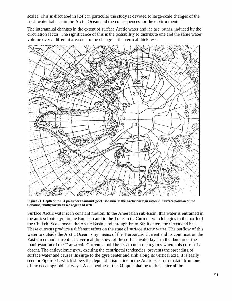
51

scales. This is discussed in [24]; in particular the study is devoted to large-scale changes of the fresh water balance in the Arctic Ocean and the consequences for the environment.

The interannual changes in the extent of surface Arctic water and ice are, rather, induced by the circulation factor. The significance of this is the possibility to distribute one and the same water volume over a different area due to the change in the vertical thickness.

Figure 21. Depth of the 34 parts per thousand (ppt) isohaline in the Arctic basin,in meters; Surface position of the isohaline; multiyear mean ice edge in March.

Surface Arctic water is in constant motion. In the Amerasian sub-basin, this water is entrained in the anticyclonic gyre in the Eurasian and in the Transarctic Current, which begins in the north of the Chukchi Sea, crosses the Arctic Basin, and through Fram Strait enters the Greenland Sea. These currents produce a different effect on the state of surface Arctic water. The outflow of this water to outside the Arctic Ocean is by means of the Transarctic Current and its continuation the East Greenland current. The vertical thickness of the surface water layer in the domain of the manifestation of the Transarctic Current should be less than in the regions where this current is absent. The anticyclonic gyre, exciting the centripetal tendencies, prevents the spreading of surface water and causes its surge to the gyre center and sink along its vertical axis. It is easily seen in Figure 21, which shows the depth of a isohaline in the Arctic Basin from data from one of the oceanographic surveys. A deepening of the 34 ppt isohaline to the center of the

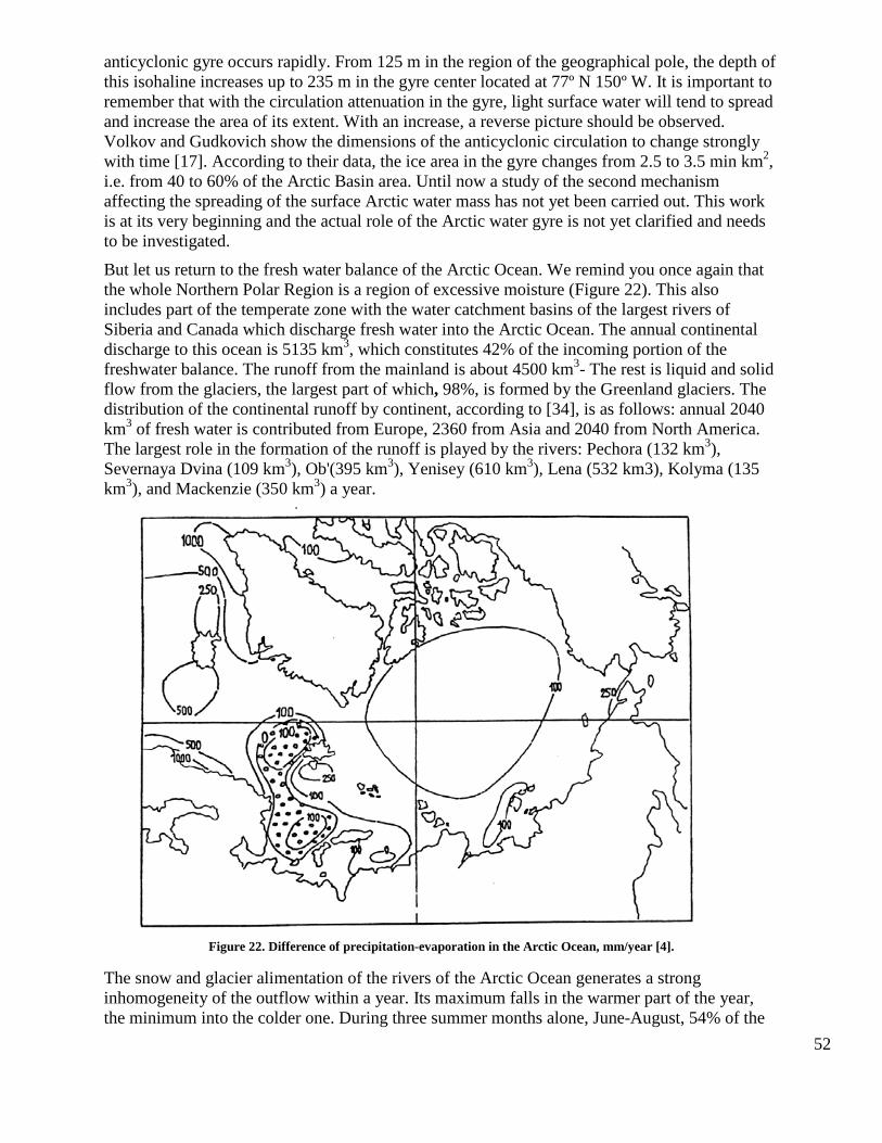
52

anticyclonic gyre occurs rapidly. From 125 m in the region of the geographical pole, the depth of this isohaline increases up to 235 m in the gyre center located at 77º N 150º W. It is important to remember that with the circulation attenuation in the gyre, light surface water will tend to spread and increase the area of its extent. With an increase, a reverse picture should be observed. Volkov and Gudkovich show the dimensions of the anticyclonic circulation to change strongly with time [17]. According to their data, the ice area in the gyre changes from 2.5 to 3.5 min km2, i.e. from 40 to 60% of the Arctic Basin area. Until now a study of the second mechanism affecting the spreading of the surface Arctic water mass has not yet been carried out. This work is at its very beginning and the actual role of the Arctic water gyre is not yet clarified and needs to be investigated.

But let us return to the fresh water balance of the Arctic Ocean. We remind you once again that the whole Northern Polar Region is a region of excessive moisture (Figure 22). This also includes part of the temperate zone with the water catchment basins of the largest rivers of Siberia and Canada which discharge fresh water into the Arctic Ocean. The annual continental discharge to this ocean is 5135 km3, which constitutes 42% of the incoming portion of the freshwater balance. The runoff from the mainland is about 4500 km3- The rest is liquid and solid flow from the glaciers, the largest part of which, 98%, is formed by the Greenland glaciers. The distribution of the continental runoff by continent, according to [34], is as follows: annual 2040 km3 of fresh water is contributed from Europe, 2360 from Asia and 2040 from North America. The largest role in the formation of the runoff is played by the rivers: Pechora (132 km3), Severnaya Dvina (109 km3), Ob'(395 km3), Yenisey (610 km3), Lena (532 km3), Kolyma (135 km3), and Mackenzie (350 km3) a year.

Figure 22. Difference of precipitation-evaporation in the Arctic Ocean, mm/year [4].

The snow and glacier alimentation of the rivers of the Arctic Ocean generates a strong inhomogeneity of the outflow within a year. Its maximum falls in the warmer part of the year, the minimum into the colder one. During three summer months alone, June-August, 54% of the

53

ocean annual value is contributed to it, while during the winter months, January-March - 7%. This feature is particularly distinct in the surface outflow from the Arctic islands. Here 80% falls during the three most water abundant months, and 3% in the months with the lowest water input. This strong irregularity in the income of fresh water during the year appreciably increases the seasonal rhythm of hydro-meteorological conditions in the marginal ocean domain.

The continental outflow into the Arctic Ocean also experiences noticeable interannual and multiyear changes. This is shown by the data of the annual outflow for the period of 1918-1967, given in [34]. One should remember that these data are derived by means of calculations and are not measured water transports. The calculations were made separately for each of the outflow components, and the mean multiyear values are obtained as the difference between precipitation and evaporation. The annual outflow values from the mainland were determined by multiplying the outflow norm by a modular precipitation coefficient of each year. The latter is found by one or several stations with long-term observation series in the regions with synchronous phase fluctuations. The annual values of the glacier outflow were based on the assumption that the iceberg discharge did not change during the entire time interval under study, which is equal to the mean multiyear value. The liquid outflow from the glaciers was found from the equation, which used air temperature in July-August as an argument.

Of course, the calculated outflow components derived at all these assumptions cannot be considered final, especially when one speaks about the pre war period with its sparse observation network. As to the other components of the freshwater balance of the Arctic Ocean, the situation here is even worse. This fact makes it impossible to demonstrate by means of the actual data the dependence of polar halocline on the freshwater balance in this ocean. Regretfully, due to the insurmountable technical difficulties such a possibility will not, probably, appear in the near future either. However, hoping to obtain at least preliminary evidence of the relationship between sea ice development and freshwater inflow to the Arctic Ocean on the basis of actual data, we investigated this relationship with regard to one of the freshwater balance components. This is the water inflow from the continents and its effect on the sea ice state. Let us remind you that the continental outflow comprises less than half (42%) of the incoming portion of the freshwater balance.

Figure 23 presents two curves: the upper curve is the continental outflow to the Arctic Ocean from Asia and North America from 1940 to 1968 while the lower curve is the ice cover extent in the North European Basin for 1946 to 197 1. Both curves are plotted from mean annual data. A dashed line shows the 5 years running means of the natural characteristics.

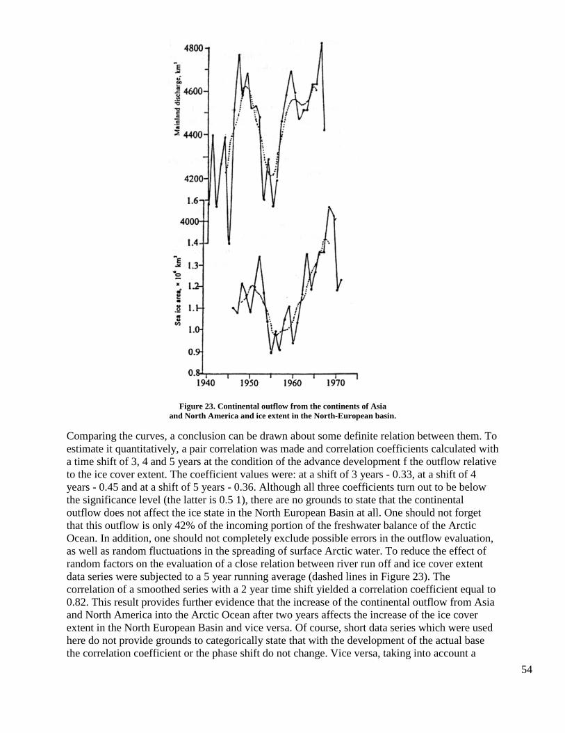
54

Figure 23. Continental outflow from the continents of Asia

and North America and ice extent in the North-European basin.

Comparing the curves, a conclusion can be drawn about some definite relation between them. To estimate it quantitatively, a pair correlation was made and correlation coefficients calculated with a time shift of 3, 4 and 5 years at the condition of the advance development f the outflow relative to the ice cover extent. The coefficient values were: at a shift of 3 years - 0.33, at a shift of 4 years - 0.45 and at a shift of 5 years - 0.36. Although all three coefficients turn out to be below the significance level (the latter is 0.5 1), there are no grounds to state that the continental outflow does not affect the ice state in the North European Basin at all. One should not forget that this outflow is only 42% of the incoming portion of the freshwater balance of the Arctic Ocean. In addition, one should not completely exclude possible errors in the outflow evaluation, as well as random fluctuations in the spreading of surface Arctic water. To reduce the effect of random factors on the evaluation of a close relation between river run off and ice cover extent data series were subjected to a 5 year running average (dashed lines in Figure 23). The correlation of a smoothed series with a 2 year time shift yielded a correlation coefficient equal to 0.82. This result provides further evidence that the increase of the continental outflow from Asia and North America into the Arctic Ocean after two years affects the increase of the ice cover extent in the North European Basin and vice versa. Of course, short data series which were used here do not provide grounds to categorically state that with the development of the actual base the correlation coefficient or the phase shift do not change. Vice versa, taking into account a

55

spatial extent of the continental outflow over the ocean perimeter, its asynchronous fluctuations and disagreement in the lag time of the outflow anomalies one can expect that the shift in time between the water inflow from continents and the ice state in the North European Basin will change within 2-4 years. Of principal importance is, however, the fact that the changes in the ice state at the Arctic Ocean border with the Atlantic occur several years after the changes in the continental water inflow. This conclusion, made from available actual data and which is, makes it difficult to disprove, appears to be extremely important both in terms of practice and science. The presence of a distinct time lag between the cause and effect has an obvious prognostic value. From a scientific standpoint this conclusion is of exceptional interest, as it establishes the order existing in nature or the order of the events and thus answers a very important question: which phenomenon is the cause and which is the effect.

Physical explanations of the order of the events in the climate system attempted in this section do not convince as well as a simple fact found from the observations. The fact that the freshwater inflow into the Arctic Ocean is the cause for the changes in sea ice extent at the border with the Atlantic, leaves no doubt about the direction of the climate signal. On the basis of this fact and a physical understanding discussed in the previous paragraphs, one can imagine the order of the signal transfer in the climate system in the following generalized form: atmosphere - ocean - sea ice - atmosphere. The water turnover in nature or to be more exact the polar branch of the hydrological cycle appears to be a specific expression of this signal.

56

Effect of the Arctic Ice on Atmospheric Circulation

It follows from the above that, under present day conditions, the changes in the area of the Arctic sea ice during the colder period of the year can be induced only by the change in the haline structure of the upper ocean layer. Indirectly, this change will also affect the thermal state of the atmosphere. In this light, the statement that sea ice can act as an active climate forming factor, generally speaking, does not appear paradoxical.

It is important to note that the ice effect on the atmosphere is not limited to the thermal effect. That it can produce a significant effect on atmospheric circulation is already evident from the fact that the Arctic anticyclone, considered by Viese [13] as a regulator of atmospheric processes in the Northern polar region, could form as a pressure formation only in the conditions of the ice regime in the Arctic. These ice conditions change with time and continue to influence the state of this anticyclone, in particular its horizontal dimensions and pressure in the centre. It is well known, for example, that during the period of sea ice area reduction and climate warming the atmospheric pressure in high latitudes decreases considerably. This was pointed out as early as 1936 by Sherhag. According to Sherhag the area of the negative pressure anomaly during this period covered the polar and subpolar areas and in some places also the zone of temperate latitudes. Villett [14] showed a pressure decrease over a significant area of the Arctic Basin, Alaska and the Canadian Arctic archipelago from 1900-1919 and 1920-1939 to reach 4 mb and more. It was less significant to the south. This process was accompanied by an increase in the speed of the western zonal flow in high latitudes: between 60º and 80º N it was at sea level for the winter season - 0.98 and for the summer - 0.6 m/s.

Also, it is known that the Arctic climate front in the atmosphere separating cold Arctic and warm polar sea air is essentially related to the ice edge. Naturally, the changes in the geographical position of this edge should induce similar changes in the position of the Arctic front and associated cyclonic activity. During the Arctic warming when ice retreated to the north, the Atlantic cyclones extended along more northern trajectories than before and after the epoch. As observed by Viese [12], data indicate that during the warming of the Arctic the cyclones coming from the north of the Atlantic shift in the Arctic and subarctic along the trajectories located much more to the north of their trajectories before the warming. This shift of cyclonic tracks to the north constitutes many hundreds and even thousands of kilometers. This conclusion was later confirmed by Vitel [15]. By comparing the indices of the pressure calculation regime of four decades (1900-1919 and 1920-1939), he found that the largest changes in the intensity of the anticyclonic circulation took place in the middle latitudes and the cyclonic circulation in the high latitudes and some in the region of the Azores. The most significant changes of the cyclonic activity occurred in the Kara Sea are. This sea is also characterized by the most appreciable ice cover extent fluctuations of a climate scale. As a result of the deviation of the trajectories to the north, the number of cyclones passing through Europe decreased by about 10% while those crossing the northern seas increased.

An important consequence of such a development of events was a decrease of atmospheric precipitation in the basins of Volga and Kama and a drop of the Caspian Sea level. This important geographical feature, relating the ice cover extent of the polar seas with the Caspian Sea level was discovered by Berg [5] after investigating the information referring to the warming epoch. However, it was possible to check its viability by the data of the climate cooling, which began at the beginning of the 1930s and 1940s. The increase of the ice cover extent in the Arctic was accompanied by atmospheric precipitation in the Barents, Kara, Leptev Seas and over much

57

of the East Siberian Sea and by increased transports at all sections of the rivers of the Volga basin [45].

Of course, neither Viese nor Vitel explained the deviations of the trajectories of the Atlantic cyclones via the effect of sea ice, as no one believed in the governing role of atmospheric circulation in the development of natural conditions. However, when new facts appeared and the understanding of the physical causes of interannual and multiyear variability of the ice area in the Arctic improved, there were grounds to consider variations of trajectories of the Atlantic cyclones as a result of the changes in sea ice distribution in the North European Basin. At least the existence of a dependence between the horizontal development of the halocline and sea ice extent during the colder part of the year makes such statement convincing enough.

Sea ice influences not only the character of atmospheric circulation but its intensity too. The most significant features of the changes of the latter during the present were widely discussed in scientific publications. As has already been mentioned, the main feature of the spatial structure of current changes in the thermal regime of the atmosphere is a distinct attenuation of the amplitude of these changes toward the equator. During climate warmings over the hemisphere thermal contrasts between high and low latitudes should decrease and zonal atmospheric circulation should increase and zonality enhance, due to this, i.e. during the coolings. Such dependence is confirmed by actual data and, in particular, by variations of the meridional temperature gradient in the latitudinal zone of 25-70º N during the present century [8].

There are also quite convincing data indicating an increase of atmospheric circulation in the Arctic during its warming (13, 14, etc.) and a decrease during the subsequent cooling [22]. In other words, in the background of the general attenuation of zonal air transports over the hemisphere during the climate warmings, there is an increase in the Arctic. The circulation increase in the Arctic becomes possible due to the shift of the trajectories of the Atlantic cyclones following the sea ice edge retreat to the north. During cooling when the edge shifts to the south there is an attenuation of the cyclonic activity in the Arctic over a background of increasing air transports on the whole over the hemisphere. Some studies have shown the regime of atmospheric precipitation, in particular in inland regions, to be closely connected with the intensity of zonal air transports. In this light, we can speak about the increase of the amount of this precipitation in the Arctic region during climate warmings and its decrease during coolings. However, for the time being it does not seem to be possible to say anything definite about the consequences of this for the ocean and its freshwater balance. It is not clear how the other components of this balance behave in the conditions of the changing moisture regime. In the meantime, clarity of this question is very much needed. We can only suggest, based on some indirect data, that with the development of warming the freshwater balance of the Arctic Ocean becomes positive. The advance in this direction will result in the "braking" of the warming processes and the development of the tendency toward the return of the system into the initial position.

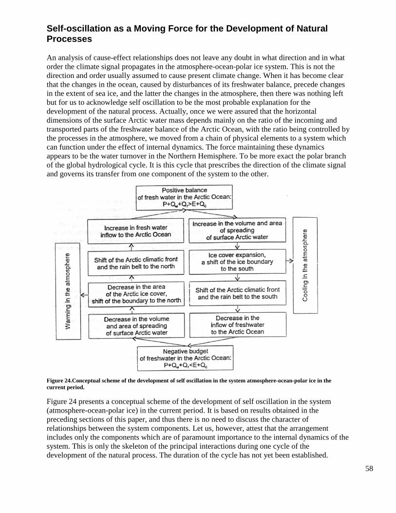
58

Self-oscillation as a Moving Force for the Development of Natural Processes

An analysis of cause-effect relationships does not leave any doubt in what direction and in what order the climate signal propagates in the atmosphere-ocean-polar ice system. This is not the direction and order usually assumed to cause present climate change. When it has become clear that the changes in the ocean, caused by disturbances of its freshwater balance, precede changes in the extent of sea ice, and the latter the changes in the atmosphere, then there was nothing left but for us to acknowledge self oscillation to be the most probable explanation for the development of the natural process. Actually, once we were assured that the horizontal dimensions of the surface Arctic water mass depends mainly on the ratio of the incoming and transported parts of the freshwater balance of the Arctic Ocean, with the ratio being controlled by the processes in the atmosphere, we moved from a chain of physical elements to a system which can function under the effect of internal dynamics. The force maintaining these dynamics appears to be the water turnover in the Northern Hemisphere. To be more exact the polar branch of the global hydrological cycle. It is this cycle that prescribes the direction of the climate signal and governs its transfer from one component of the system to the other.

Figure 24.Conceptual scheme of the development of self oscillation in the system atmosphere-ocean-polar ice in the current period.

Figure 24 presents a conceptual scheme of the development of self oscillation in the system (atmosphere-ocean-polar ice) in the current period. It is based on results obtained in the preceding sections of this paper, and thus there is no need to discuss the character of relationships between the system components. Let us, however, attest that the arrangement includes only the components which are of paramount importance to the internal dynamics of the system. This is only the skeleton of the principal interactions during one cycle of the development of the natural process. The duration of the cycle has not yet been established.

59

Depending on the form of freshwater as it returns to the Arctic Ocean - mainly in the form of atmospheric precipitation over this ocean, iceberg, or surface runoff from Eurasia and North America - this duration can vary from several months to several years. Also, it is necessary to mention that the relationship between separate components of the system (atmosphere-ocean-polar ice) has been investigated only at the qualitative level. Possibly, this is the maximum of what can be done today, considering the state of the observation base. For the same reason, the interaction between some of the system components has been investigated today only approximately at a qualitative level. This concerns, particularly, the dependence of the freshwater balance of the Arctic Ocean on the character of atmospheric circulation. At the same time, it is difficult to argue that during the periods of sea ice cover expansion and atmospheric coolings, when there is a southward shift of the belt of west winds and intensive rains, the reduction of moisture inflow to the Arctic Ocean occurs. During the reduction of the ice area and atmospheric warming, the moisture inflow to the Arctic is, vice versa, increased. That is why the block in the conceptual system, which reflects the change in the fresh water inflow to the polar ocean, does not appear to be purely theoretical.

The ability of the atmosphere-ocean-polar ice system to function in a self contained regime does not exclude the effect of exterior factors. The changes of carbon dioxide and aerosols in the atmosphere, solar insulation, and solar activity levels can affect the thermodynamical state of the atmosphere and, hence, the regime of self oscillation. They can enhance, draw out, and in general distort the character of these oscillations itself. But these external factors can appreciably influence the development of sea ice and cause the effect of polar forcing only through this system. They are incorporated in it and go through a number of successive transformations.

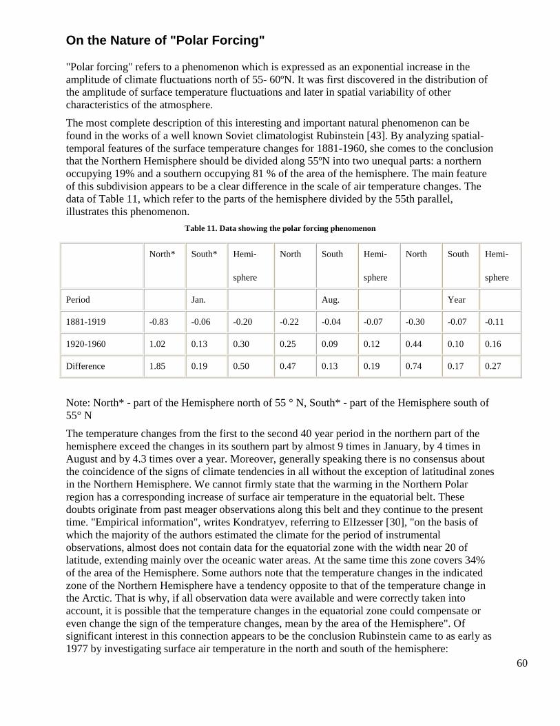
60

On the Nature of "Polar Forcing"

"Polar forcing" refers to a phenomenon which is expressed as an exponential increase in the amplitude of climate fluctuations north of 55- 60ºN. It was first discovered in the distribution of the amplitude of surface temperature fluctuations and later in spatial variability of other characteristics of the atmosphere.

The most complete description of this interesting and important natural phenomenon can be found in the works of a well known Soviet climatologist Rubinstein [43]. By analyzing spatial-temporal features of the surface temperature changes for 1881-1960, she comes to the conclusion that the Northern Hemisphere should be divided along 55ºN into two unequal parts: a northern occupying 19% and a southern occupying 81 % of the area of the hemisphere. The main feature of this subdivision appears to be a clear difference in the scale of air temperature changes. The data of Table 11, which refer to the parts of the hemisphere divided by the 55th parallel, illustrates this phenomenon.

Table 11. Data showing the polar forcing phenomenon

North* South* Hemi-

sphere

North South Hemi-

sphere

North South Hemi-

sphere

Period Jan. Aug. Year

1881-1919 -0.83 -0.06 -0.20 -0.22 -0.04 -0.07 -0.30 -0.07 -0.11

1920-1960 1.02 0.13 0.30 0.25 0.09 0.12 0.44 0.10 0.16

Difference 1.85 0.19 0.50 0.47 0.13 0.19 0.74 0.17 0.27

Note: North* - part of the Hemisphere north of 55 ° N, South* - part of the Hemisphere south of 55° N

The temperature changes from the first to the second 40 year period in the northern part of the hemisphere exceed the changes in its southern part by almost 9 times in January, by 4 times in August and by 4.3 times over a year. Moreover, generally speaking there is no consensus about the coincidence of the signs of climate tendencies in all without the exception of latitudinal zones in the Northern Hemisphere. We cannot firmly state that the warming in the Northern Polar region has a corresponding increase of surface air temperature in the equatorial belt. These doubts originate from past meager observations along this belt and they continue to the present time. "Empirical information", writes Kondratyev, referring to ElIzesser [30], "on the basis of which the majority of the authors estimated the climate for the period of instrumental observations, almost does not contain data for the equatorial zone with the width near 20 of latitude, extending mainly over the oceanic water areas. At the same time this zone covers 34% of the area of the Hemisphere. Some authors note that the temperature changes in the indicated zone of the Northern Hemisphere have a tendency opposite to that of the temperature change in the Arctic. That is why, if all observation data were available and were correctly taken into account, it is possible that the temperature changes in the equatorial zone could compensate or even change the sign of the temperature changes, mean by the area of the Hemisphere". Of significant interest in this connection appears to be the conclusion Rubinstein came to as early as 1977 by investigating surface air temperature in the north and south of the hemisphere:

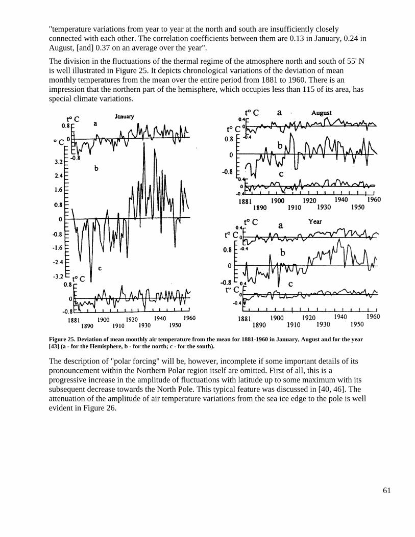
61

"temperature variations from year to year at the north and south are insufficiently closely connected with each other. The correlation coefficients between them are 0.13 in January, 0.24 in August, [and] 0.37 on an average over the year".

The division in the fluctuations of the thermal regime of the atmosphere north and south of 55' N is well illustrated in Figure 25. It depicts chronological variations of the deviation of mean monthly temperatures from the mean over the entire period from 1881 to 1960. There is an impression that the northern part of the hemisphere, which occupies less than 115 of its area, has special climate variations.

Figure 25. Deviation of mean monthly air temperature from the mean for 1881-1960 in January, August and for the year [43] (a - for the Hemisphere, b - for the north; c - for the south).

The description of "polar forcing" will be, however, incomplete if some important details of its pronouncement within the Northern Polar region itself are omitted. First of all, this is a progressive increase in the amplitude of fluctuations with latitude up to some maximum with its subsequent decrease towards the North Pole. This typical feature was discussed in [40, 46]. The attenuation of the amplitude of air temperature variations from the sea ice edge to the pole is well evident in Figure 26.

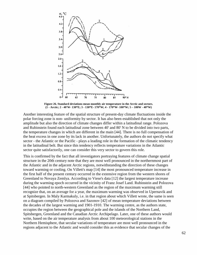
62

Figure 26. Standard deviations mean monthly air temperature in the Arctic and sectors. (1 - Arctic; 2 - 40'W- 130*E; 3 - 130*E- 170*W; 4 - 170*W- 100*W; 5 – 100W - 40*W)

Another interesting feature of the spatial structure of present-day climate fluctuations inside the polar forcing zone is non- uniformity by sector. It has also been established that not only the amplitude but also the direction of climate changes differ within a latitudinal range. Polozova and Rubinstein found each latitudinal zone between 40' and 80' N to be divided into two parts, the temperature changes in which are different in the main [44]. There is no full compensation of the heat excess in one zone by its lack in another. Unfortunately, the authors do not specify what sector - the Atlantic or the Pacific - plays a leading role in the formation of the climatic tendency in the latitudinal belt. But since this tendency reflects temperature variations in the Atlantic sector quite satisfactorily, one can consider this very sector to govern this role.

This is confirmed by the fact that all investigators portraying features of climate change spatial structure in the 20th century note that they are most well pronounced in the northernmost part of the Atlantic and in the adjacent Arctic regions, notwithstanding the direction of these changes toward warming or cooling. On Villett's map [14] the most pronounced temperature increase in the first half of the present century occurred in the extensive region from the western shores of Greenland to Novaya Zemlya. According to Viese's data [12] the largest temperature increase during the warming epoch occurred in the vicinity of Franz Josef Land. Rubinstein and Polozova [44] who pointed to north-western Greenland as the region of the maximum warming still recognize that, on an average for a year, the maximum warming was observed in Upernavik and at Spitsbergen. In Maly Karmakuly, i.e. in that region about which Villett wrote, the same is seen on a diagram compiled by Polozova and Sazonov [42] of mean temperature deviations between the decades of the largest warming and 1901-1910. The warming centre, as the authors state, occupies the region between the geographical pole and the islands of the Northern Land, Spitsbergen, Greenland and the Canadian Arctic Archipelago. Later, one of these authors would write, based on the air temperature analysis from about 100 meteorological stations in the Northern Hemisphere, that secular variations of temperature are most well pronounced in the regions adjacent to the Atlantic and would consider this as evidence that secular changes of the

63

atmosphere thermal regime are connected in some way with the ocean. Le Roi Laduri probably had the same in mind when he wrote that the warming of the first half of the 20th century occurred mainly in the countries of the North Atlantic coasts [32]. There are many quotations of such, indicating a special sensitivity of the North Atlantic and the Atlantic sector of the Arctic to climate changes. They all vary a little, indicating that while high latitudes play a special role in climate changes over the hemisphere, the Atlantic sector of the Arctic plays a special role in these latitudes themselves. This important aspect of the spatial structure of polar forcing should not, of course, be omitted when explaining the causes of the present day climate changes.

Palaeographic data referring to the Quaternary Period indicate that the localization of this source changed little in the main, at least over the last 0.7 m1n. years. This was the time when the gigantic ice sheets appeared and were dissolved on the continents of Europe and North America, when the entire physical-geographical situation on the Earth experienced radical rhythmical changes, extreme by scales. The character of these changes on the Earth's surface is quite well studied now. The scales of the current changes and the changes during the glacial period are incomparable, but the extent of inhomogeneities in space remains mainly constant.

The description of these inhomogeneities in climate development and in general of natural conditions in the Pleistocene, based on the analysis of vast palaeogeographical material, is contained in the fundamental work of Markov and Velichko [33]. We present, without great detail, the conclusions of these authors. There were, first of all, comparatively small changes in natural conditions from the glacial to interglacial periods along the equatorial belt of the Earth. Secondly, there was an increase in the amplitude of fluctuations toward the centers of ancient ice sheets located in high and temperate latitudes on both sides of the Atlantic. Thirdly, irregular latitudinal variability was augmented and complicated by irregular sector variability and the sector variances were most pronounced in these latitudes. "In the European sector they reached 50° C, and in the East Siberian one - only 5° C, i.e. were 10 fold less" [33].

These conclusions, as we see it, repeat all that has already been said with regard to spatial inhomogeneities of the current climate changes over the Northern Hemisphere. Of course, during the glacial epochs when the shift and deformation involved practically all climate belts, the belt of maximum climate changes shifted from the Arctic to the temperate latitudes. But it is important that the North Atlantic and the Atlantic sector of the Arctic in general preserve importance as the center of climate disturbances of some kind over the hemisphere during the entire last stage of the glacial period. This circumstance suggests that the causes for the vast climate changes in the Pleistocene possibly preserved its significance in our days too.

Another circumstance, very important in our opinion for the understanding of the "polar forcing" nature, is the extent of synchronization of climate fluctuations within the forcing area itself and outside it. Is the time lag in the development of some or other climate oscillation in the hemisphere real?

Polozova and Rubinstein, who studied the character of the "Arctic warming" manifestation, came to the conclusion that "on an average for a year the maximum warming was noted in Upernavik, at Spitsbergen and in Maly Karmakuly and extended to the east and south and west with decreasing intensity". They formulate this conclusion more definitely. "Thus, they write, "the warming probably extended mainly from west to east with a significant inertia of 5- 10 years. This inertia increased in the process of the warming spreading southward: the warming peak shifts to later years with a decrease of latitude…". It is important to note that the cooling, which replaced the warming process again according to their data, began in the region where the warming was most intensive. East, west, and south of this region the onset of cooling shifted to later years.

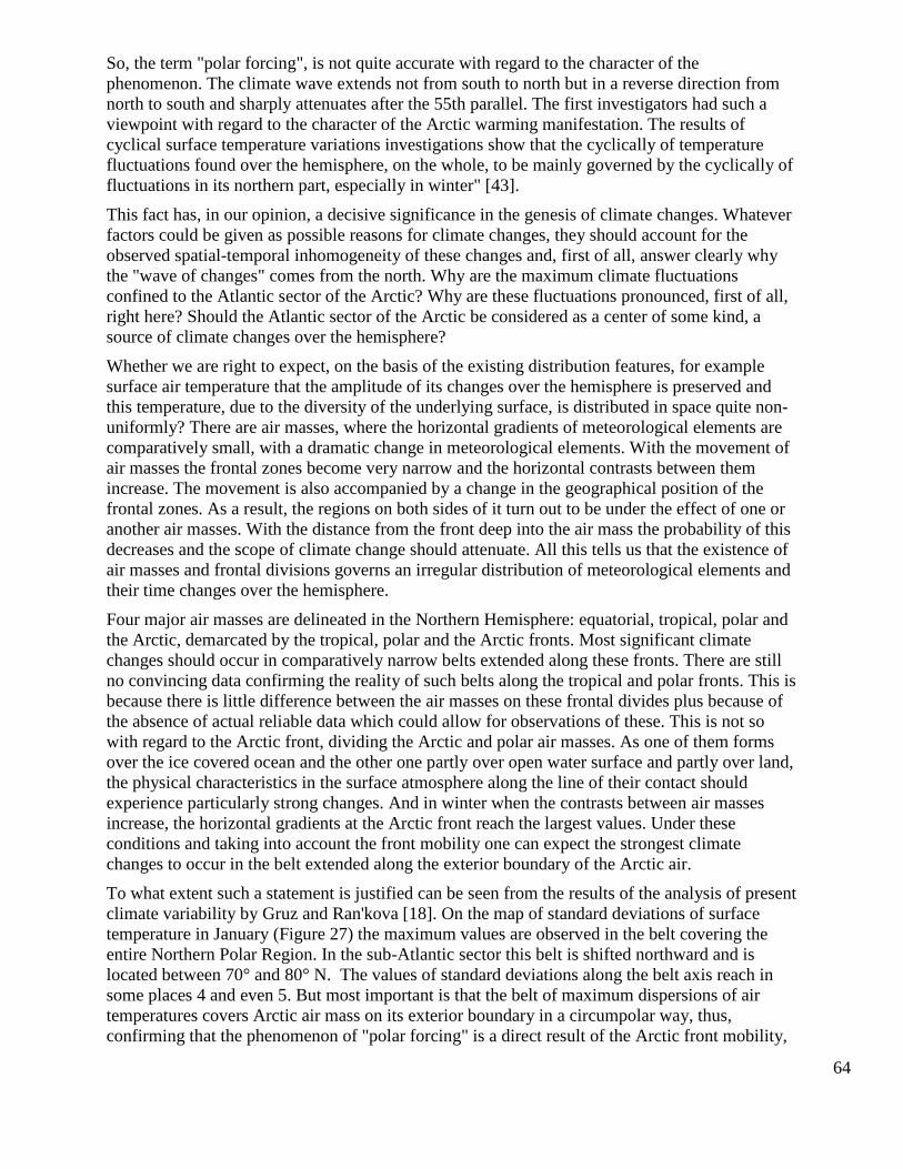
64

So, the term "polar forcing", is not quite accurate with regard to the character of the phenomenon. The climate wave extends not from south to north but in a reverse direction from north to south and sharply attenuates after the 55th parallel. The first investigators had such a viewpoint with regard to the character of the Arctic warming manifestation. The results of cyclical surface temperature variations investigations show that the cyclically of temperature fluctuations found over the hemisphere, on the whole, to be mainly governed by the cyclically of fluctuations in its northern part, especially in winter" [43].

This fact has, in our opinion, a decisive significance in the genesis of climate changes. Whatever factors could be given as possible reasons for climate changes, they should account for the observed spatial-temporal inhomogeneity of these changes and, first of all, answer clearly why the "wave of changes" comes from the north. Why are the maximum climate fluctuations confined to the Atlantic sector of the Arctic? Why are these fluctuations pronounced, first of all, right here? Should the Atlantic sector of the Arctic be considered as a center of some kind, a source of climate changes over the hemisphere?

Whether we are right to expect, on the basis of the existing distribution features, for example surface air temperature that the amplitude of its changes over the hemisphere is preserved and this temperature, due to the diversity of the underlying surface, is distributed in space quite non-uniformly? There are air masses, where the horizontal gradients of meteorological elements are comparatively small, with a dramatic change in meteorological elements. With the movement of air masses the frontal zones become very narrow and the horizontal contrasts between them increase. The movement is also accompanied by a change in the geographical position of the frontal zones. As a result, the regions on both sides of it turn out to be under the effect of one or another air masses. With the distance from the front deep into the air mass the probability of this decreases and the scope of climate change should attenuate. All this tells us that the existence of air masses and frontal divisions governs an irregular distribution of meteorological elements and their time changes over the hemisphere.

Four major air masses are delineated in the Northern Hemisphere: equatorial, tropical, polar and the Arctic, demarcated by the tropical, polar and the Arctic fronts. Most significant climate changes should occur in comparatively narrow belts extended along these fronts. There are still no convincing data confirming the reality of such belts along the tropical and polar fronts. This is because there is little difference between the air masses on these frontal divides plus because of the absence of actual reliable data which could allow for observations of these. This is not so with regard to the Arctic front, dividing the Arctic and polar air masses. As one of them forms over the ice covered ocean and the other one partly over open water surface and partly over land, the physical characteristics in the surface atmosphere along the line of their contact should experience particularly strong changes. And in winter when the contrasts between air masses increase, the horizontal gradients at the Arctic front reach the largest values. Under these conditions and taking into account the front mobility one can expect the strongest climate changes to occur in the belt extended along the exterior boundary of the Arctic air.

To what extent such a statement is justified can be seen from the results of the analysis of present climate variability by Gruz and Ran'kova [18]. On the map of standard deviations of surface temperature in January (Figure 27) the maximum values are observed in the belt covering the entire Northern Polar Region. In the sub-Atlantic sector this belt is shifted northward and is located between 70° and 80° N. The values of standard deviations along the belt axis reach in some places 4 and even 5. But most important is that the belt of maximum dispersions of air temperatures covers Arctic air mass on its exterior boundary in a circumpolar way, thus, confirming that the phenomenon of "polar forcing" is a direct result of the Arctic front mobility,

65

its temporal fluctuations. Let us note that the most significant features in the distribution of standard deviations, typical of January, are clearly observed during the eight cold months from October to May. That is why we see the same picture on the map, referring to the year on the whole, The region of maximum deviation is extended latitudinally between 60° and 80° N from Baffin Land in the west to the New Siberian Islands in the east with the values of 1.0, and in some places 1.5° C. The other, smaller area of the maximum temperature variability is located in the Pacific coast of Alaska. Together they form a belt of enhanced climate variability at the exterior boundary of the Arctic air mass.

Figure 27. Maps of standard deviations of surface air temperature north of 20° N on the whole for the year (a) and in January (b), according to Gruza and Ran'kova [18].

In light of the above discussions on the nature of polar forcing, is it possible to explain the main features of the current climate change over the hemisphere and, in particular, the localization of the most significant changes in the Atlantic sector of the Arctic?

As compared with the Southern Hemisphere, where the sea ice boundary contacts open water surface everywhere, the Arctic sea ice has such contact only in the Atlantic sector. North of Siberia, Alaska, and the islands of the Arctic Archipelago it approaches very closely the shore during 9- 10 months and is located near it the remaining time. Naturally, in these conditions the Arctic front which forms at the conjunction of polar sea air and Arctic air cannot be continuous. It should break in those regions where sea ice is adjacent to the shore. Within the Atlantic sector of the Arctic, the Arctic front has two branches: the Atlantic beginning south of Greenland extending through the Norwegian and Barents Seas to the Kara Sea and the North American one, going from the southern tip of Greenland to north west of Baffin Land. The Atlantic branch breaks in the Kara Sea and the North American one in the Boothia Peninsula area. Thus, an enhanced sensitivity of the Atlantic sector of the Arctic to climate changes is attributed to the

66

presence of the mobile Arctic front here, dividing two contrasting air masses: the Arctic and the Polar Sea. If the front line were continuous and not broken, then instead of a separate although vast area in the Atlantic sector of the Arctic one could find a belt of strong climate fluctuations covering the entire high latitudinal zone.

67

Conclusion

There is a deep internal relationship between the formation, extent, and stability of ice in deep sea and its upper layer structure. This relationship suggests the possibility for two typical regimes in the Arctic, ice free and ice regimes. The transition from the first regime to the second one occurs as a result of a change in the vertical water column structure accompanied by the halocline formation near the ocean surface. Strongly restricting the vertical heat exchange, the halocline creates the necessary conditions for ice formation everywhere, where annual heat losses by the ocean exceed its income from the Sun, i.e. in the regions of energy discharge. And the development of the halocline mass governs the geographical distribution and the most significant features of the Arctic ice cover configuration. The transition from the ice regime to the ice free regime occurs when the halocline disappears. The advective heat, incoming to the Arctic Ocean in the system of the North Atlantic Current, attains in this case unrestrained energy exchange with the atmosphere and is capable not only of melting the existing ice but preventing new ice formation. Thus, the question of ice cover stability in the Arctic appears to be the question of stability of the current vertical structure of its water column, whether the halocline is present or absent. Since the latter results from distinct variances in the salinity of the surface and underlying water masses, the halocline will be preserved until these exist.

On the other hand, the changes of the halocline zone over time, induced by a disturbed freshwater balance of the Arctic Ocean, should be accompanied by corresponding sea ice area changes. For the ice to completely cover the Greenland and Barents Sea in winter, it is sufficient if desalinated Arctic water spreads over them. The present thermal conditions in the atmosphere cannot serve as a factor restraining the horizontal development of the ice cover. The reduction of the halocline dimensions with the dominance of the fresh water outflow from the Arctic Ocean over its income will be, vice versa, accompanied by a decrease of the Arctic ice area. Taking into account the presence of the correlation between sea ice development and thermal conditions in the atmosphere we can suggest that sea ice area variations were an immediate direct cause for the two largest climate fluctuations in the Arctic in the present century.

Among the factors causing the disturbance of the fresh water balance in the Arctic Ocean most important, undoubtedly, appears to be the change in the moisture turnover in the atmosphere, induced by the deviations of prevailing cyclone trajectories in connection with the dynamics of the exterior sea ice boundary. Most certainty reliable data disclosing the relation of moisture turnover in the atmosphere with the ice state in the Arctic are quite scarce. However, the order of the climate signal transfer in the climate system, when changes in the ocean induced by the disturbances of its freshwater balance precede changes in sea ice extent, and the latter precede changes in the atmosphere, suggests that self oscillation is the most probable cause for the development of natural processes at the present time. The idea, that the internal dynamics of the climate system are the main moving force in the development of the natural process, was used to account for vast glacial-interglacial fluctuations in the Pleistocene.

68

References

1. Aleksandrov, E.I., et. al. 1986. Climate structure and variability of the

Northern Polar region, Obninsk: VNIIGMI VIDC, 8, 64 p.p.

2. Alekseyev, G.V. and P.N. Svyashennikov. 1991. Natural variability of climate

characteristics of the Northern Polar Region and the Northern Hemisphere, L.,

Gidrometeoizdat, 160 p.p.

3. Abramov, B.A. and V.F. Zakharov. 1985. Dependence of thermal conditions in the

atmosphere on sea ice development in the Arctic, Proc.of the AARI, 400, 60-72.

4. 1980. Atlas of the oceans, The Arctic Ocean,. MO VMF

5. Berg, L.C. Climate and life. M., Gos. geograf. literatury, 356 p.p.

6. Brooks, Ch. 1947. Climates of the past, M., Inost-annaya literatura, 1952, 358 p.p.

7. Budyko, M.I. 1969. Polar ice and climate. L., Gidrometeoizdat 36 p.p.

8. Budyko, M.I. 1971. Climate and life. L., Gidrometeoizdat, 472 p.p.

9. Bulgakov, N.P. 1963. Ice. /fMe Pacific Ocean [Editor’s note: Illegible from the original]

10. Bulgakov, N.P. 1975. Convection in the ocean. M., Nauka, 272 p.p.

11. Burova, L.P. 1983. Moisture turnover in the Arctic atmosphere. L., Gidrometeoizdat, 128

p.p.

12. Viese, V. Yu. 1940. Climate of the seas of the Soviet Arctic. M. L., Glavsevmorput, 124

p.p.

13. Viese, V. Yu. 1944. Bases of long-term ice forecasts for the Arctic Seas. M.,

Glavsevmorput, 274 p.p.

14. Villett, H.K. 1966. Character of the relationship between solar and climate phenomena.

Solar activity and climate changes, L., Gidrometeoizdat, 23-43 p.p.

15. Vitel's, L.A. 1948. Multiyear changes of the pressure-circulation regime and their effect

on climate fluctuations. Proceedings of GGM. 8(70), 51-109.

16. Vinnikov, K.Ya. 1986. Climate sensitivity. L., Gidrometeoizdat, 224 p.p.

17. Volkov, N.A. and Z.M. Gudkovich. 1967. Main results of the ice drift studies in the

Arctic Basin. Problemy Arktiki i Antarktiki. 27, 55-64.

18. Gruza, G.V. and E. Ya Ran'kova. 1979. Data on the climate structure and variability. Air

temperature at sea level. The Northern Hemisphere. Obninsk,. 204 p.p.

19. Doronin, Yu. P. 1968. To the problem of removing the Arctic ice. Problemy Arktiki i

Antarktiki, 28, 21-28.

69

20. Doronin, Yu.P. 1969. Thermal interaction between atmosphere and hydrosphere in the

Arctic. L., Gidrometeoizdat, 300 p.p.

21. Doronin, Yu. P., Smetannikova A.V. 1967. Effect of meteorological factors on the dates

of ice formation. Proceedings of the AARI, 257, 45-56.

22. Zakharov, V.F. 1976. Cooling of the Arctic and the ice cover of the Arctic Seas.

Proceedings of the AARI, 337, 96 p.p.

23. Zakharov, V.F. 1977. Ice age categories of the Arctic Ocean. Proceedings of the AARI.

346, 118-121.

24. Zakharov. V.F. 1978. The World Ocean and glacial epochs of the Pleistocene. L.,

Gidrometeoizdat, 64 p.p.

25. Zakharov. V.F. 198 1. Ice of the Arctic and current natural processes. L.

Gidrometeoizdat, 136 p.p.

26. Zakharov. V.F. and L.A. Strokina. 1978. Present day changes of the ice cover of the

Arctic Ocean. Meteorologiia i Gidrologiia.7, 35-43.

27. Zubov. N.N. 1948. In the center of the Arctic. M.L., Glavsevmorput, 392 p.p.

28. Ivanov. V.V. 1976. Freshwater balance of the Arctic Ocean. Proceedings of the AARI.

323, 138-147.

29. Climate regime of the Arctic at the border of XX and = centuries. 1991. L.,

Gidrometeoizdat, 200 p.p.

30. Kondratyev, K.Ya. 1991. Global climate and its changes. L., Nauka, 1987, 232 p.p.

31. Laktionov, A.R. 1955. The North Pole. M., Morskoi transport, 472 p.p.

32. Le Roi Laduri, E. 1971. Climate history from 1000. L., Gidrometeoizdat, 280 p.p.

33. Markov, K.K. and A.A. Velichko. 1967. Quaternary period. M., Nedra,. V. Ill. 440 p.p.

34. 1974. The world water balance and water resources of the Earth. L., Gidrometeoizdat,

638 p.p.

35. Monitoring of the Arctic climate. 1988. L., Gidrometeoizdat, 224 p.p.

36. Nazintsev, Yu.L. 1961. Heat loss through the ice cover in the central Arctic. Problemy

Arktiki i Antarktiki, 8, 36-46.

37. Nikiforov, Ye.G. and A.O. Shpaikher. 1980. Typical formation features of large-scale

fluctuations of the hydrological regime of the Arctic Ocean. L., Gidrometeoizdat, 252

p.p.

38. Nikolayeva, A.Ya. and N.P. Shesterikov. 1970. Method for calculating ice conditions by

the example of the Laptev Sea. Proceedings of the AARI, 292, 143-217.

70

39. Sea Ice Nomenclature. 1974. L., Gidrometeoizdat, 76 p.p.

40. Unintentional impact on climate. 1974. L., Gidrometeoizdat, 260 p.p.

41. Panov, V.V. and A.O. Shpaikher. 1963. Effect of Atlantic water on some features of the

hydrological regime of the Arctic Basin and adjacent seas. HOceanology. V.3. 4, 579-

590.

42. Polozova, L.G. and B.I. Sazonov. 1968. On the possible cause of the modem warming of

the Arctic Izv. AN SSSR, ser. geograf., 4, 99-105.

43. Rubinstein, Ye. S. 1977. Structure of air temperature fluctuations over the Northern

Hemisphere. L., Gidrometeoizdat, P.1, 1973, P.11, 36 and 28 p.p.

44. Rubinstein, Ye. S. and L.G. Polozova. 1966. Currents climate change. L.,

Gidrometeoizdat, 268 p.p.

45. Sarukhanyan, E.I. and N.P. Smimov. 1971. Multiyear variations of the Volga outflow. L.,

Gidrometeoizdat, 166 p.p.

46. Smimov N.P., et. al. 1988. Monitoring of the thermal regime of the Arctic. Monitoring of

the Arctic climate, L., Gidrometeoizdat, 24-32 p.p.

47. Timofeyev, V.T. 1960. Water masses of the Arctic Basin.L.,Gidrometeoizdat,192p.p.

48. Treshnikov, et al. 1967. Heat exchange of the Southern Ocean with the atmosphere.

Problemy Arktiki i Antarktiki, 27,35-47.

49. Treshnikov, A.F. and G.I. Baranov. 1972. Water circulation structure in the Arctic Basin.

L., Gidrometeoizdat, 158 p.p.

50. Vowinkel, E. and C. Orvig. 1973. Climate of the Arctic Basin. Climate of polar regions,

L., Gidrometeoizdat, 170-317 p.p.

51. Bourke, R.H. and R.P. Garrett. 1987. Sea ice thickness distribution in the Arctic Ocean.

HCold Regions Science and Technology, V. 13, 3, 259- 280.

52. Bergthorsson, P. 1969. An estimate of drift ice and temperature of Iceland in 1000 Years.

Jokul 1, 19, 94- 10 1.

53. Dunbar, M. and W. Wittmann. 1962. Some features of ice movements in the Arctic

Basin. Proc. Arctic sympos., 90-108 p.p.

54. Gloersen, P. and W.J. Campbell. 1988. Variations in the Arctic, Antarctic and Global sea

ice covers during 1978-1987 as observed with the Nimbus scanning multichannel

microwave radiometer. J. of Geophysical Res. V.93, 9C, 10666-10674.

55. Isforholdene i de Arctiske Have (Ice conditions in the Arctic Ocean). 1898-1939.

19461956. Danish Meteorological Institute.

71

56. Koerner, P.M. 1971. Ice balance in the Arctic Ocean. IIAIDJEX Bull, 6,11-26.

57. Lyon, W. 1966. Under surface of sea ice observed from submarine. I/Physics of snow and

ice proceedings of the Conference. V.1, Part 1. Hokkaido Univ. 1967.

58. Malmberg, S. 1969. Hydrographic changes in the waters between Iceland and Jan Mayen

in the last decade. IIJokull, 19, 30-43.

59. Malmberg, S. 1971. Annual and seasonal hydrographic variations in the East Iceland

current between Iceland and Jan Mayen. IISea Ice, Proceedings of an International

Conference., Reykjavik, 42-54.

60. Parkinson, C.L. et al. 1987. Arctic sea ice, 1973-1976: Satellite passive microwave

observations, NASA Spec. Publ. SP-489, 296 p.p.

61. 1988. Report of 30 Years of Observation of Sea Ice by Marine Department, JMA, Tokyo,

96p.p.

62. Steffansson, V. 1969. Temperature variations in the North Icelandic coastal area during

recent decades.//Jokull, 19, 18-28.

63. Swithinbank, C. 1972. Arctic pack ice from below. II Sea Ice. Proceedings of an

International Conference, Reykjavik, May 10-13, 1971,246-254.

64. Thoroddsen, P. n.d. Arferdi a Islandi i 1000 ar. Copenhagen, 1916-1917.

65. Wadhams, P. 1981. The Ice Cover in the Greenland and Norwegian Seas. IlReviews of

Geophysics and Space Physics. V.19, 3, 345-393.

66. Wittmann, W.I. and J.J. Schule. 1966. Comments of the Mass Budget Arctic Pack Ice.

I/Processes of the Arctic Heat Budget and Atmospheric Circulation. The Rand

Corporation.