General rights Copyright and moral rights for the publications made accessible in the public portal are retained by the authors and/or other copyright owners and it is a condition of accessing publications that users recognise and abide by the legal requirements associated with these rights.

Users may download and print one copy of any publication from the public portal for the purpose of private study or research.

You may not further distribute the material or use it for any profit-making activity or commercial gain

You may freely distribute the URL identifying the publication in the public portal If you believe that this document breaches copyright please contact us providing details, and we will remove access to the work immediately and investigate your claim.

Downloaded from orbit.dtu.dk on: Dec 15, 2021

Second-order theory for coupling 2D numerical and physical wave tanks: Derivation,evaluation and experimental validation

Yang, Zhiwen; Liu, Shuxue; Bingham, Harry B.; Li, Jinxuan

Published in:Coastal Engineering

Link to article, DOI:10.1016/j.coastaleng.2012.07.003

Publication date:2013

Document VersionPublisher's PDF, also known as Version of record

Link back to DTU Orbit

Citation (APA):Yang, Z., Liu, S., Bingham, H. B., & Li, J. (2013). Second-order theory for coupling 2D numerical and physicalwave tanks: Derivation, evaluation and experimental validation. Coastal Engineering, 71, 37-51.https://doi.org/10.1016/j.coastaleng.2012.07.003

Coastal Engineering 71 (2013) 37–51

Contents lists available at SciVerse ScienceDirect

Coastal Engineering

j ourna l homepage: www.e lsev ie r .com/ locate /coasta leng

Second-order theory for coupling 2D numerical and physical wave tanks:Derivation, evaluation and experimental validation

Zhiwen Yang a,b,⁎, Shuxue Liu a,1, Harry B. Bingham b,2, Jinxuan Li a

a State Key Laboratory of Coastal and Offshore Engineering, Dalian University of Technology, Dalian 116023, Chinab Department of Mechanical Engineering, Technical University of Denmark, DK-2800 Kgs. Lyngby, Denmark

⁎ Corresponding author. Fax: +45 4588 4325.E-mail addresses: ouyangzhiwen@gmail.com (Z. Yan

hbb@dtu.mek.dk (H.B. Bingham), lijx@dlut.edu.cn (J. Li)1 Fax: +86 411 84708526.2 Fax: +45 4588 4325.

0378-3839/$ – see front matter © 2012 Elsevier B.V. Allhttp://dx.doi.org/10.1016/j.coastaleng.2012.07.003

a b s t r a c t

a r t i c l e i n f o

Article history:Received 29 February 2012Received in revised form 9 June 2012Accepted 29 July 2012Available online 30 August 2012

Keywords:Second-order couplingNumerical wave tanksPhysical wave tanksWavemaker theory

A full second-order theory for coupling numerical and physical wave tanks is presented. The ad hoc unifiedwave generation approach developed by Zhang et al. [Zhang, H., Schäffer, H.A., Jakobsen, K.P., 2007. Deter-ministic combination of numerical and physical coastal wave models. Coast. Eng. 54, 171–186] is extendedto include the second-order dispersive correction. The new formulation is presented in a unified form thatincludes both progressive and evanescent modes and covers wavemaker configurations of the piston- andflap-type. The second order paddle stroke correction allows for improved nonlinear wave generation in thephysical wave tank based on target numerical solutions. The performance and efficiency of the new modelis first evaluated theoretically based on second order Stokes waves. Due to the complexity of the problem,the proposed method has been truncated at 2D and the treatment of regular waves, and the re-reflectioncontrol on the wave paddle is also not included. In order to validate the solution methodology further, aseries of nonlinear, periodic waves based on stream function theory are generated in a physical wave tankusing a piston-type wavemaker. These experiments show that the new second-order coupling theory pro-vides an improvement in the quality of nonlinear wave generation when compared to existing techniques.

© 2012 Elsevier B.V. All rights reserved.

1. Introduction

Deterministic models have increasingly been used by coastal engi-neers for combining numerical and physical wave tanks. Indeed, thisapproach allows the numerical model to focus on wave propagationin the offshore region and the physical model to treat the wave trans-formation in the near-shore region. Wave generation in the physicalmodel completely utilizes the calculated wave motions by a suitablenumerical model along with the boundary data connecting the twomodels and considers the asymmetry and nonlinearity of the progres-sive wave. The data transfer between the two models is built uponreal-time nonlinear wave motion instead of stochastic parameterssuch as significant wave height and peak period. Consequently, thisapproach exploits the advantages of numerical and physical modelingto provide an improved description of full-scale, realistic engineeringproblems.

Initial efforts in this direction include Zhang and Schäffer (2004)and Zhang and Schäffer (2007) for wave flumes, and Zhang andSchäffer (2005) for the theoretical aspects in 3D. The most advanced

g), liusx@dlut.edu.cn (S. Liu),.

rights reserved.

theory developed for this purpose is referred to as the ad hoc unifiedwave generation theory (Zhang et al., 2007), which blends linear,fully dispersive wavemaker theory with a nonlinear, shallow waterwave generation approach. In this method, the wave paddle controlsignal is calculated from a nonlinear shallow wavemaker differenceequation and then corrected with a linear dispersion parameter.This method has been experimentally verified to be well suited forgeneration of small amplitude waves in all water depths and fornonlinear shallow water waves. The method's performance deterio-rates however for nonlinear waves in intermediate or deep water.In order to extend the range of application of this method, Yang etal. (2011b) proposed a real-time correction method to correct theerror which is produced in the hydrodynamic frameworks and themechanical system of wavemaker. However, while the dispersioncorrection or the real-time correction in previous studies are basedon linear wavemaker theory, the evanescent modes are not accountedfor in the paddle signals which renders them inadequate for correctingthe high harmonic components which appear when generating highlynonlinear or relatively deep water waves. Quite recently Yang et al.(2011a) developed an approximate second-order coupling theorywhich pushes the limits of application from shallowwater to relativelydeep water, but this theory did not include the evanescent modes.Moreover, the previous models collectively ignored the unwantedspurious free waves in the physical tank. Therefore, in this paper weintroduce a new second-order coupling theory for numerical andphysical wavemodels which includes the evanescent modes. Relevant

38 Z. Yang et al. / Coastal Engineering 71 (2013) 37–51

analyses regarding the generation and the corresponding suppressionefficiency of the spurious free waves have also been addressed.

Since the accuracy of a coupling model mainly depends on the as-sumption of wave paddle motion and the description of the resultantphysical wave field, we are motivated to extend the model to includesecond-order wavemaker theory. Second-order wavemaker theoryhas a long history of development going back at least to Fontanet(1961) for regular waves. Ottesen-Hansen et al. (1980), Sand (1982)and Sand and Donslund (1985) discussed the second-order long wavegeneration in the laboratory. Hudspeth and Sulisz (1991) derived thecomplete second-order Eulerian theory for waves generated by amonochromatic wave paddle motion with special emphasis on Stokesdrift and return flow in wave flumes. In addition, Flick and Guza(1980) and Sulisz and Hudspeth (1993) addressed the effects of spuri-ous super-harmonic waves. In seeking an explanation of these effects,Schäffer (1996) derived a complete second-order model includingboth sub- and super-harmonics. This full theory successfully predictsthe second-order motion of the wave paddle required to produce aspatially homogeneous wave field at second order. In this study, weapply the complete second-order wavemaker theory given by Schäffer(1996), except that we only consider regular (monochromatic) waves.The extension to irregular waves is the subject of ongoing work.

In the present model, the first- and second-order solutions for thewave paddle position are obtained by combining wavemaker theorywith a fully nonlinear, depth-integrated flux based on a numericalmodel. This development is based on a classical perturbation ap-proach combined with Taylor expansion of the boundary conditionson the free surface, which is formulated in a unifying form that in-cludes both progressive and evanescent mode and covers wavemakerconfigurations of the piston- and flap‐type. Except being restrictedby the inherent limitations of second-order Stokes wave theory, thistheory does not assume the primary waves to be restricted by a narrowfrequency band, shallow water, or small amplitude. With a second-order dispersion correction and the consideration of evanescent modesin the control signal, this new formulation allows the physical modelto capture more accurately the high order behavior of nonlinear wavemotion.

The derivation and effectiveness of the new formulation havebeen evaluated numerically by considering a theoretical second-order Stokes wave. To test the limits of the method, we attempt togenerate a wide range of nonlinear waves based on stream functiontheory using a piston-type wavemaker and compare with the originalmodel of Zhang and Schäffer (2007). For better comparison of the ac-curacy and efficiency of the present model with the previous method,no attempt is made to consider re-reflection control on the wave pad-dle, so that all the wavemaker signals are based solely on the calculatedwave paddle position. These experiments show that the newmodel hasa wider range of applicability than existing wave generation methods.

The remainder of this paper is structured as follows. In Section 2the formulation of the second-order coupling theory are given.Section 3 describes a recipe for the generation of the complete control

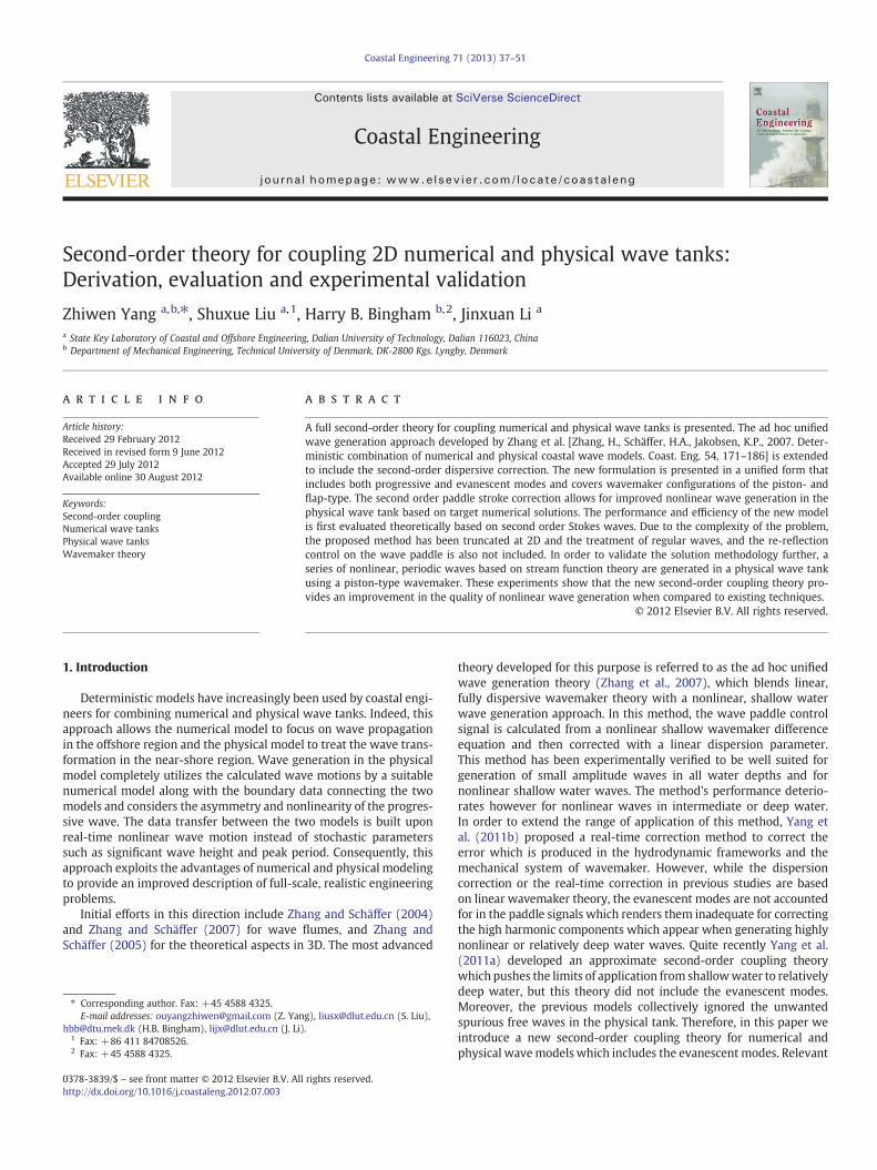
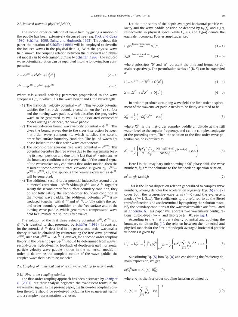
Fig. 1. Definition sketch of the coupled system

coupling signal including a general procedure of the connection be-tween the numerical and physicalmodel and the solution of the couplingdifference equation. Section 4 presents a numerical analysis on therelevant first- and second‐order coupling parameters. Section 5 evalu-ates the model in terms of the suppression of spurious second-orderfree waves and the accuracy and efficiency of the proposed numericalscheme for solving the coupling equations. Section 6 discusses therange of application. Experimental validation is provided in Section 7.Finally, conclusions are drawn in Section 8.

2. Modeling the second-order coupling wave field

2.1. General description

The geometry of the coupling model is illustrated in Fig. 1. Thesimulation area is divided into a numerical field Ω1 and a physicalfield Ω2. Ω1 represents the far wave field which allows numericalwaves to be generated and propagate into the physical model, andΩ2 indicates the near-shore area with the complex physics wherethe physical waves are generated from a coupled wavemaker signalbased on the numerical wave information. Any suitable theory or nu-merical wave model can be used in the far field Ω1. It is clear that thekernel of the coupling problem is the data transformation betweenthe two models, i.e., how to obtain accurately the wave paddle signalsfrom a given numerical wave in order that the physical waves canproceed successfully in Ω2.

In order to fully understand the complexity of the data transfor-mation, the wavemaker has to be considered as a coupled system.In this context, it is important to appreciate the following. Applyinga single-frequency, sinusoidal signal to the wave paddle in Ω2 willcause it to move and generate a wave field. This wave field induceshydrodynamic feedback, such as wave surface elevation or velocity,around the wave board. The nature of this hydrodynamic feedbackis dependent on the full nonlinearity of the numerical waves at theboundary of the two fields and it is this nonlinear hydrodynamicfeedback that determines, via the paddle controller, the position tobe applied at the next time step. Zhang et al. (2007) has proposed afirst-order coupling approach, namely the ad hoc unified wavemakertheory, coupling provided by the depth-averaged horizontal particlevelocity based on a linear wave theory. In this paper, however, we ex-tend this method to include the second-order dispersive correction byforcing the moving wave paddle to match the second-order boundarycondition between the two models. Consequently, for each time stept, numerical and physical model must satisfy the matching conditionat a specific location x, i.e.,

UP x; tð Þ≡UN x; tð Þ ð1Þ

where, subscripts “N” and “P” represent the numerical and physical so-lution, respectively, U the depth-averaged horizontal particle velocity.

of numerical and physical wave models.

39Z. Yang et al. / Coastal Engineering 71 (2013) 37–51

2.2. Induced waves in physical field Ω2

The second order calculation of wave field by giving a motion ofthe paddle has been extensively discussed see (e.g. Flick and Guza,1980; Schäffer, 1996; Sulisz and Hudspeth, 1993). Throughout thispaper the notation of Schäffer (1996) will be employed to describethe induced waves in the physical field Ω2. With the physical wavefield known, the coupling relation between the numerical and physi-cal model can be determined. Similar to Schäffer (1996), the inducedwave potential solution can be separated into the following four com-ponents:

ϕ ¼ εϕ 1ð Þ þ ε2ϕ 2ð Þ þ O ε3� �

ð2� aÞ

ϕ 2ð Þ ¼ ϕ 21ð Þ þ ϕ 22ð Þ þ ϕ 23ð Þ ð2� bÞ

where ε is a small ordering parameter proportional to the wavesteepness H/L, in which H is the wave height and L the wavelength.

(1) The first-order velocity potential— ϕ(1): This velocity potentialsatisfies the first-order boundary condition on the free surfaceand the moving wave paddle, which describes the progressivewave to be generated as well as the associated evanescentmodes arising at, or near, the wave paddle.

(2) The second-order bound wave velocity potential — ϕ(21): Thisgives the bound waves due to the cross-interaction betweenfirst-order wave components, which satisfies the secondorder free surface boundary condition. The bound waves arephase locked to the first order wave components.

(3) The second-order spurious free wave potential — ϕ(22): Thispotential describes the free waves due to the wavemaker leav-ing its mean position and due to the fact that ϕ(2l) mismatchesthe boundary condition at the wavemaker. If the control signalof the wavemaker only contains a first-order motion, then theresultant second-order surface elevation is given by ϕ(2)=ϕ(2l)+ϕ(22), i.e., the spurious free waves expressed as ϕ(22)

will be generated.(4) The additional second-order potential induced by second order

numerical correction— ϕ(23): Although ϕ(2l) and ϕ(22) togethersatisfy the second order free surface boundary condition, theydo not fully satisfy the second-order boundary condition atthe moving wave paddle. The additional potential ϕ(23) is in-troduced, together with ϕ(2l) and ϕ(22), to fully satisfy the sec-ond order boundary condition on the free surface and at themoving wave paddle, which generates a compensated wavefield to eliminate the spurious free waves.

The solution of the first three velocity potential, ϕ(l), ϕ(2l) andϕ(22), is identical to that presented by Schäffer (1996). In contrast,for the potential ϕ(23) described in the pure second-order wavemakertheory, it can be obtained by counteracting the free wave potential,ϕ(22), such that ϕ(23)=−ϕ(22). However, for a second order couplingtheory in the present paper, ϕ(23) should be determined from a givensecond-order hydrodynamic feedback of depth-averaged horizontalparticle velocity wave paddle motion in the numerical model. Inorder to determine the complete motion of the wave paddle, thecoupled wave field has to be modeled.

2.3. Coupling of numerical and physical wave field up to second order

2.3.1. First-order coupling solutionThe first-order coupling approach has been discussed by Zhang et

al. (2007), but their analysis neglected the evanescent terms in thewavemaker signal. In the present paper, the first-order coupling solu-tion therefore should be re-derived including the evanescent terms,and a complex representation is chosen.

Let the time series of the depth-averaged horizontal particle ve-locity and the wave paddle position be denoted by U0(t), and X0(t),respectively, in physical space, while Ua(ω), and Xa(ω) denote theequivalent complex Fourier amplitudes, i.e.,

U0 tð Þ ⇔Fourier transform

Ua ωð Þ ð3� aÞ

X0 tð Þ ⇔Fourier transform

Xa ωð Þ ð3� bÞ

where subscripts “0” and “a” represent the time and frequency do-main respectively. The perturbation series of (U, X) can be expandedas

U ¼ εU 1ð Þ þ ε2U 2ð Þ þ O ε3� �

ð4� aÞ

X ¼ εX 1ð Þ þ ε2X 2ð Þ þ O ε3� �

: ð4� bÞ

In order to produce a coupling wave field, the first-order displace-ment of the wavemaker paddle needs to be firstly assumed to be

X 1ð Þ0 ¼ 1

2−iX 1ð Þ

a eiωt þ c:c:n o

ð5Þ

where Xa(1) is the first-order complex paddle amplitude at the still

water level, ω the angular frequency, and c.c. the complex conjugateof the preceding term. Then the solution to the first-order wave po-tential can be expressed as

ϕ 1ð Þ ¼ 12

igX 1ð Þa

ω

X∞j¼0

cjcoshkj zþ hð Þ

coshkjhei ωt−kjxð Þ þ c:c:

8<:

9=; ð6Þ

Here i is the imaginary unit showing a 90° phase shift, the wavenumbers, kj, are the solutions to the first-order dispersion relation,

ω2 ¼ gkj tanhkjh ð7Þ

This is the linear dispersion relation generalized to complex wavenumbers, where g denotes the acceleration of gravity. Eqs. (6) and (7)cover both the progressive-wave term (j=0) and the evanescentmodes (j=1, 2,…). The coefficients cj, are referred to as the Biéseltransfer function, and are determined by requiring the solution to sat-isfy the boundary conditions at the wavemaker which are formulatedin Appendix A. This paper will address two wavemaker configura-tions: piston-type (l→∞) and flap-type (l=0), see Fig. 1.

According to the first-order velocity potential and applying theboundary condition Eq. (1), the relation between the numerical andphysical models for the first-order depth-averaged horizontal particlevelocities is given by

U 1ð ÞN ¼ U 1ð Þ

P ¼ 1h∫0−hϕ

1ð Þx

x¼0dz ¼

12

ωX 1ð Þa

X∞j¼0

cjkjh

eiωt þ c:c:

8<:

9=;

������ ð8Þ

Substituting Eq. (5) into Eq. (8) and considering the frequency do-main expression, we get,

ωX 1ð Þa ωð Þ ¼ Λ1j ωð Þ⋅U 1ð Þ

N;a ð9Þ

where Λ1j is the first-order coupling function obtained by

Λ1j ωð Þ ¼X∞j¼0

cjkjh

þ c:c:

24

35−1

ð10Þ

40 Z. Yang et al. / Coastal Engineering 71 (2013) 37–51

which includes both the progressive part and the evanescent modes.For j=0, i.e. without evanescent terms, Eq. (10) gives the realquantityΛ10 which is known as the transfer function Λ in Zhang etal. (2007). For j=1, 2,…, Λ1j is purely imaginary.

Eq. (9) gives a frequency-domain relation between the wave pad-dle position for the physical model and the first-order componentof the depth-averaged particle velocity exported from a numericalmodel. In practice, this is readily converted to the time domain. Forconvenient conversion, as in Zhang et al. (2007), it can firstly be re-written as two equations

ωX 1ð Þa;sw ωð Þ ¼ U 1ð Þ

N;a ð11� aÞ

X 1ð Þa ωð Þ ¼ Λ1j ωð Þ·X 1ð Þ

a;sw ωð Þ ð11� bÞ

By means of the assumption of the first-order wave paddle mo-tion, Eq. (5), the time-domain form can also be expressed as

dX 1ð Þ0;sw tð Þdt

¼ U 1ð ÞN;0 tð Þ ð12� aÞ

X 1ð Þ0 tð Þ ¼ F−1 Λ1j ωð Þ·F X 1ð Þ

0;sw tð Þh ih i

ð12� bÞ

where F−1 and F represent the inverse and forward Fourier trans-form, respectively. They are evaluated in practice via the Fast FourierTransform (FFT). The subscript “sw” indicates the use of shallowwater theory for obtaining the paddle position, since Eq. (12-a) isconsistent with the idea which is widely applied in shallow longwave generation (see e.g. Synolakis, 1990). UN,0

(1) denotes the time se-ries of first-order depth-averaged particle velocity exported from anumerical model or a suitable wave theory. Eq. (12-a) formulates areal-time link between the numerical and physical models underthe assumption of shallowwater. Eq. (12-b) gives a first-order disper-sion correction needed when deviating from the shallow water limit.Consequently, without the evanescent modes, Eqs. (12-a) and (12-b)are identical to the ad hoc unified wavemaker theory proposed byZhang et al. (2007).

2.3.2. Second-order coupling solutionAt second order, the idea will be consistent with the first order

coupling solution, i.e., to seek the relation between the wave paddleposition for the physical model and the depth-averaged particle ve-locity exported from a numerical model. The velocity potential ϕ(21)

and ϕ(22) are identical to those of Schäffer (1996), which will becited directly. With the present study limited to regular waves, onlythe superharmonics are important, i.e.,

ϕ 21ð Þ ¼ 12

iX 1ð Þ2a

2

X∞j¼0

X∞l¼0

Hþjl

Dþjl

cjclcosh kj þ kl

� �zþ hð Þ

cosh kj þ kl� �

hei 2ωt−kjx−klxð Þ þ c:c:

8<:

9=;

ð13Þ

and

ϕ 22ð Þ ¼ 12

igc20X1ð Þ2a

2hω

X∞p¼0

c 22ð Þþp

coshKþp zþ hð Þ

coshKþp h

ei 2ωt−Kþp xð Þ þ c:c:

( )ð14Þ

with Hjl+, Djl

+, Kp+ and cp

(22)+ given in Appendix A.For the potential ϕ(23) described in Schäffer (1996) in a pure

second-order wavemaker theory, it can be obtained by counteractingthe free wave potential, ϕ(22)±, such that ϕ(23)±=−ϕ(22)±. But, for asecond-order coupling theory as in the present study, ϕ(23), should bedetermined from the given second-order wave paddle motion bymatching the second-order numerical wave field. This quantity, in

fact, cannot be obtained directly since the second-order wave paddlemotion is unknown. Therefore, analogous to the first-order problem,we firstly assume the second-order paddle motion as

X 2ð Þ0 ¼ 1

2−iX 2ð Þ

a e2iωt þ c:c:n o

ð15Þ

where Xa(2) denotes the second-order complex paddle amplitude at

still water level, then ϕ(23) will be obtained by

ϕ 23ð Þ ¼ 12

igX 2ð Þa

2ω

X∞p¼0

c 23ð Þþp

coshKþp zþ hð Þ

coshKþp h

ei 2ωt−Kþp xð Þ þ c:c:

( )ð16Þ

where cp(23)+ is given in Appendix A.

Similar to the separation of the velocity potential, the givensecond-order depth-averaged particle velocity in a numerical modelcan also be separated into the following three terms,

U 2ð ÞN ¼ U 21ð Þ

N þ U 22ð ÞN þ U 23ð Þ

N : ð16Þ

Making the depth-averaged integration of ϕx(2) at x=0 in the same

way as for ϕx(1) in Eq. (8), and considering Eq. (4-a) and the boundary

condition of Eq. (1), the relation between the second-order depth-averaged horizontal particle velocity in the numerical model and thesecond-order wave paddle position in physical models can be derivedas

U 21ð ÞN ¼ 1

2X 1ð Þ2a

2h

X∞j¼0

X∞l¼0

Hþjl cjcl tanh kj þ kl

� �h

Dþjl

e2iωt þ c:c:

8<:

9=; ð17� aÞ

U 22ð ÞN ¼ 1

22c20ωX 1ð Þ2

a

h

X∞p¼0

c 22ð Þþp

Kþp h

e2iωt þ c:c:

( )ð17� bÞ

U 23ð ÞN ¼ 1

22ωX 2ð Þ

a

X∞p¼0

c 23ð Þþp

Kþp h

e2iωt þ c:c:

( )ð17� cÞ

Notice that once Xa(1) in first-order problem is known, UN

(21) andUN(22) can be obtained. Applying the assumption of Eq. (15), UN

(23)

can now be determined from

U 23ð ÞN ¼ 2iωX 2ð Þ

0

X∞p¼0

c 23ð Þþp

Kþp h

þ c:c:

( )ð18Þ

Combining Eqs. (17-a), (17-b), and (17-c) with Eq. (18) gives

2ωX 2ð Þa ωð Þ ¼ Λ2p ωð Þ· U 2ð Þ

N;a−ν12 ωð Þh i

ð19Þ

where Λ2p is the second-order coupling coefficient given by

Λ2p ωð Þ ¼X∞p¼0

c 23ð Þþp

Kþp h

þ c:c:

" #−1

: ð20Þ

As before, Λ20 represents the real, and Λ2p (p=1, 2…) the purelyimaginary. v12(ω) is the complex cross-order depth-averaged particlevelocity, found from

ν12 ωð Þ ¼ λ2 ωð ÞX 1ð Þa ·X 1ð Þ

a ð21Þ

41Z. Yang et al. / Coastal Engineering 71 (2013) 37–51

with

λ2 ωð Þ ¼ 12h

X∞j¼0

X∞l¼0

Hþjl

Dþjl

cjcl tanh kj þ kl� �

hþ 2c20ωh

X∞p¼0

c 22ð Þþp

Kþp h

þ c:c:

8<:

9=;:

ð22Þ

Note that λ2(ω) is the term in the cross-order coupling coefficientwhich depends on the relative water depth and contains the interac-tion between the first- and second‐order problems.

Considering the solution in the frequency domain, as in thefirst-order problem, Eq. (19) can be split into two equations

2ωX 2ð Þa;sw ωð Þ ¼ U 2ð Þ

N;a−ν12 ωð Þ ð23� aÞ

X 2ð Þa ωð Þ ¼ Λ2p ωð Þ·X 2ð Þ

a;sw ωð Þ ð23� bÞ

with the corresponding expressions in the time domain given by

dX 2ð Þ0;sw tð Þdt

¼ U 2ð ÞN;0 tð Þ−ν12 tð Þ ð24� aÞ

X 2ð Þ0 tð Þ ¼ F−1 Λ2p ωð Þ·F X 2ð Þ

0;sw tð Þh ih i

: ð24� bÞ

Here subscript “sw” again refers to the shallow water solution.Eq. (24-b) gives a second-order dispersion correction needed whendeviating from the shallow water limit. The complete wave paddlemotion in the physical model is now

X0 tð Þ ¼ X 1ð Þ0 tð Þ þ X 2ð Þ

0 tð Þ: ð25Þ

The full second-order coupling theory between the numerical andphysical models has now been derived. It represents a unifying andcompact form that includes both progressive and evanescent modecontributions and includes wavemakers of the piston- and flap‐type.

3. Implementation

Now that we have derived the coupling model up to second order,we will give the recipe for the generation of the complete couplingcontrol signal. There are three aspects that have to be addressed.Whilst the first question involves the general procedure of thepresented second-order coupling from a numerical model to a physi-cal model, the second problem relates to the decomposition of thedepth-averaged particle velocity and the last aspect deals with thesolution of the coupling equation.

It is well known from the ad hoc wavemaker theory (Zhang et al.,2007; see also Yang et al., 2011b) that there are three steps to get acoupling control signal. Firstly, a suitable numerical model is usedto simulate wave propagation from the far field to the boundarybetween the numerical and physical models. Then the time series ofdepth-averaged particle velocity at the connecting boundary mustbe determined, in which the first- and second-order componentshave to be calculated (from Eq. (26) to Eqs. (27-a) and (27-b)). Secondly,

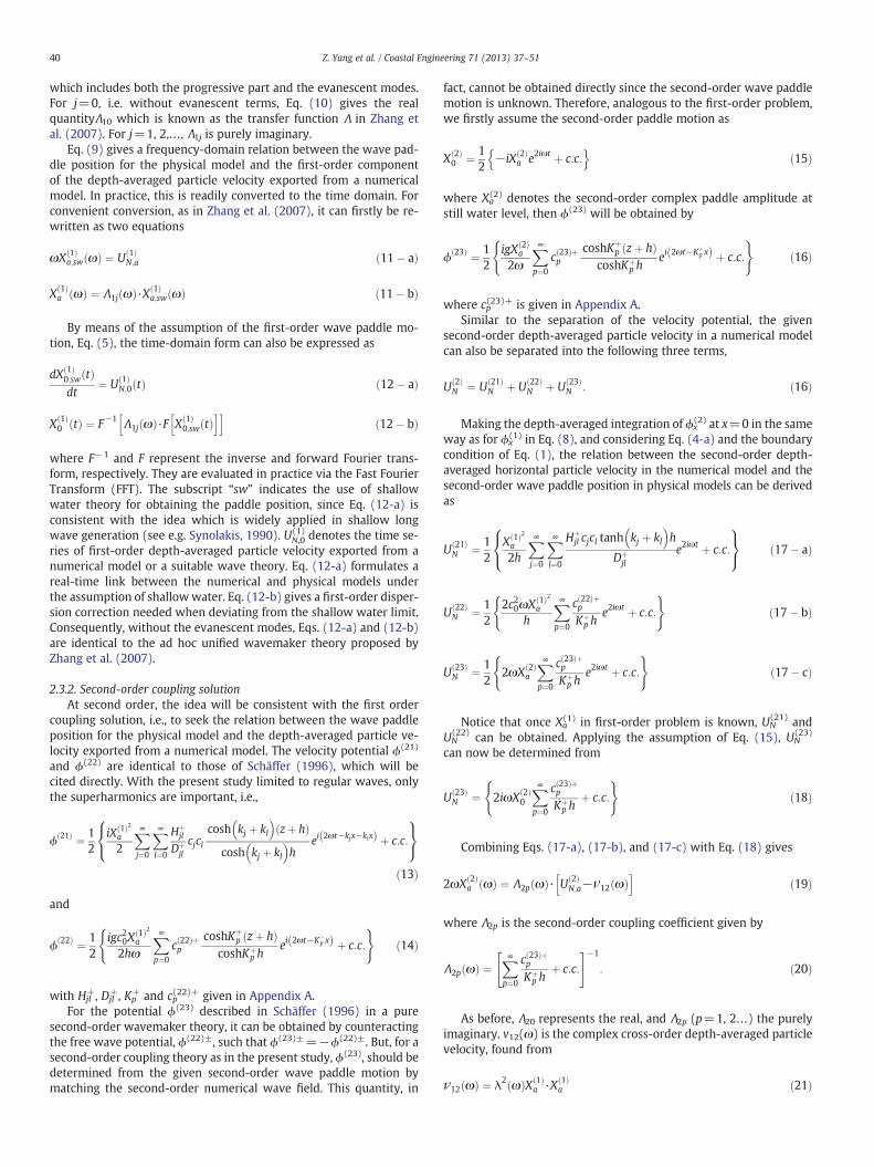
Fig. 2. General procedure of th

thefirst- and second-order components of control signalwill be obtainedto provide the total second-order signal in the time domain. Finally, thephysical wave is generated using the complete wavemaker signal. Thedetailed description is given in Fig. 2 which provides a general proce-dure of the new control mode (double-headed and continuous lines).Fig. 2 also shows the first-order coupling control mode, i.e., the ad hocunified wavemaker theory of Zhang et al. (2007) (single-headed anddotted line). Itmust be kept inmind that in thefirst-order coupling con-trol mode, the control signal can be calculated directly from Eqs. (12-a)and (12-b) by taking the first-order component of depth-averaged ve-locity, U(1) to be the total velocity, U.

For calculating the wave paddle position, various mathematicaltools could be employed to exactly decompose the total depth-averaged particle velocity U calculated from the numerical modelinto its first- and second-order components, U(1) and U(2). In thispaper, a frequency-spectrum Fourier analysis method is adopted.Converting the depth-average velocity from the time domain to thefrequency domain, we get

U tð Þ ¼ Re∑jΔje

i ωj tþφjð Þ with eiφjΔj ¼12π

∫tU tð Þe�iωj tdt ð26Þ

in which Δj and φj correspond to the amplitude and phase compo-nent, respectively, of the depth-averaged particle velocity U in thefrequency-domain at radian frequency ωj. For the regular wave casethe phase can be set asφj≡0. Then the first- and second-order solutionsin the time domain can be determined by taking the second- andfirst-order component in frequency domain to be 0, respectively, andusing an inverse Fourier transform, i.e.

U 1ð Þ tð Þ ¼ F−1Δ1; ω ¼ ω10; ω ¼ ω2⋯ others

8<:

35

24 ð27� aÞ

U 2ð Þ tð Þ ¼ F−10; ω ¼ ω1Δ2; ω ¼ ω20; others

8<:

35:

24 ð27� bÞ

Finally, we consider the solution of the coupling equation. Thedepth averaged velocity U(t) in Eqs. (12-a) and (24-a) are modifiedaccordingly as U(X0,sw(t), t) in order to include the effect of the wavepaddle position to yield

dX rð Þ0;sw tð Þdt

¼ U rð Þ X rð Þ0;sw tð Þ; t

� �: ð28Þ

Note that Eq. (28) is a nonlinear equation with “r” representingeither first- or second-order. Since the numerical model may nothave many grid points distributed over the range of the moving pad-dle, the nonlinear term U(X0,sw(t), t), was interpolated by Zhang(2005) using a ‘spline’ method to smooth out the distribution of thevelocity near the moving paddle. They also used the explicit forwardEuler (1st order) scheme for the discretization of time derivativeterms. Furthermore, in order to avoid a slow drift of the paddle dueto the discrepancy between the exact signals and the numerical

e coupling control modes.

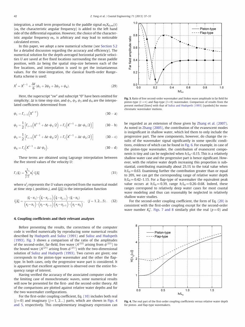
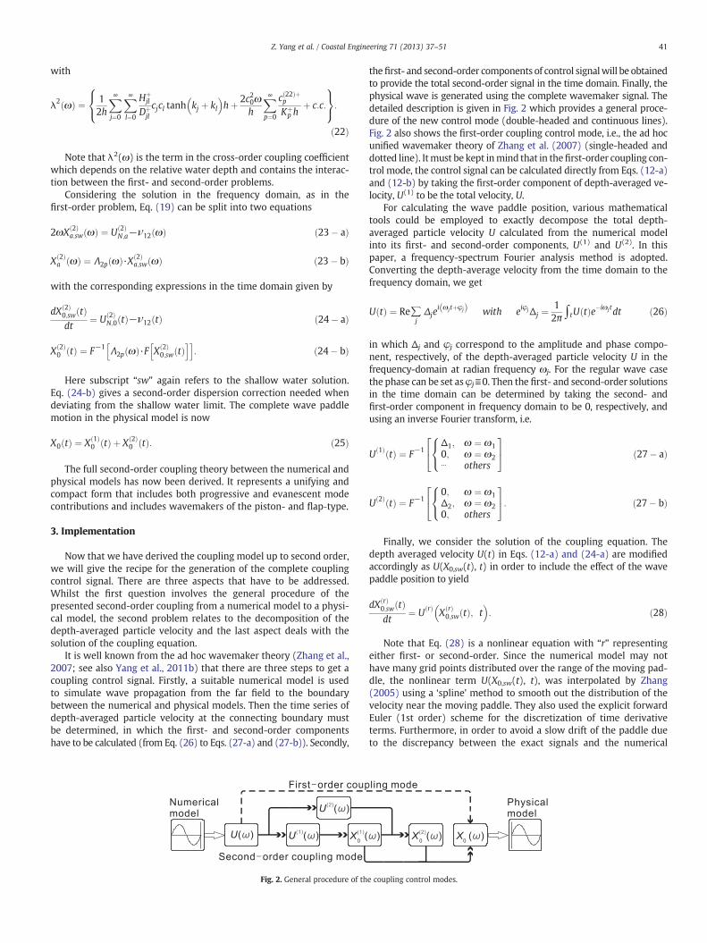
Fig. 3. Ratio of free second-order wavemaker and Stokes wave amplitude in far field forpiston-type (l→∞) and flap-type (l=0) wavemaker. Comparison of results from thepresent method [lines] with that of Sulisz and Hudspeth (1993) [symbols] for mono-chromatic wavemaker motions.

Fig. 4. The real part of the first-order coupling coefficients versus relative water depthfor piston- and flap-type wavemakers.

42 Z. Yang et al. / Coastal Engineering 71 (2013) 37–51

integration, a small term proportional to the paddle signal ωcX0,sw(t)(ωc the characteristic angular frequency) is added to the left handside of the differential equation. However, the choice of the character-istic angular frequency ωc, is arbitrary and may lead to noticeablecalculated errors.

In this paper, we adopt a new numerical scheme (see Section 5.2for a detailed discussion regarding the accuracy and efficiency). Thenumerical solution for the depth-averaged horizontal particle veloci-ties U are saved at five fixed locations surrounding the mean paddleposition, with Δx being the spatial step-size between each of thefive locations, and interpolation is used to get the instantaneousvalues. For the time-integration, the classical fourth-order Runge–Kutta scheme is used:

Xi ¼ Xi−1 þ Δt6

ψ1 þ 2ψ2 þ 2ψ3 þ ψ4ð Þ: ð29Þ

Here, the superscript “sw” and subscript “0” have been omitted forsimplicity; Δt is time step size, and ψ1, ψ2, ψ3 and ψ4 are the interpo-lated coefficients determined from

ψ1 ¼ Γ i−1 Xi−1� �

ð30� aÞ

ψ2 ¼ 12

Γ i−1 Xi−1 þ Δt·ψ1=2� �

þ Γ i Xi−1 þ Δt·ψ1=2� �h i

ð30� bÞ

ψ3 ¼ 12

Γ i−1 Xi−1 þ Δt·ψ2=2� �

þ Γ i Xi−1 þ Δt·ψ2=2� �h i

ð30� cÞ

ψ4 ¼ Γ i Xi−1 þ Δt⋅ψ3

� �: ð30� dÞ

These terms are obtained using Lagrange interpolation betweenthe five stored values of the velocity U:

Γ i ξð Þ ¼X5j¼1

uij·lj ξ½ � ð31Þ

where uij represents the U values exported from the numerical model

at time step i, position j, and lj[ξ] is the interpolation function

lj ξ½ � ¼ξ−x1ð Þ⋯ ξ−xj−1

� �ξ−xjþ1

� �⋯ ξ−x5ð Þ

xj−x1� �

⋯ xj−xj−1

� �xj−xjþ1

� �⋯ xj−x5� � ; j ¼ 1;2…5ð Þ : ð32Þ

4. Coupling coefficients and their relevant analyses

Before presenting the results, the correctness of the computercode is verified numerically by reproducing some numerical resultsdescribed by Hudspeth and Sulisz (1991) and Sulisz and Hudspeth(1993). Fig. 3 shows a comparison of the ratio of the amplitudesof the second-order, far-field, free wave (A(22) arising from ϕ(22)) tothe bound wave (A(21) arising from ϕ(21)) with the two-dimensionalsolution of Sulisz and Hudspeth (1993). Two curves are given; onecorresponds to the piston-type wavemaker and the other the flap-type. In both cases, only the progressive wave part is considered. Itis apparent that excellent agreement is observed over the entire fre-quency range of interest.

Having verified the accuracy of the associated computer code forthe limiting case of monochromatic waves, some numerical resultswill now be presented for the first- and the second‐order theory. Allof the comparisons are plotted against relative water depths and forthe two wavemaker configurations.

For the first-order coupling coefficient, Eq. (10) includes both real(j=0) and imaginary (j=1, 2…) parts, which are shown in Figs. 4and 5, respectively. This complementary imaginary expression can

be regarded as an extension of those given by Zhang et al. (2007).As noted in Zhang (2005), the contribution of the evanescent modesis insignificant in shallow water, which led them to only include theprogressive part. The new components, however, do change the re-sults of the wavemaker signal significantly in some specific condi-tions, evidence of which can be found in Fig. 6. For example, in case ofthe piston-type wavemaker, the contribution of evanescent compo-nents is tiny and can be neglected when h/L0b0.15. This is a relativelyshallow water case and the progressive part is hence significant. How-ever, with the relative water depth increasing this proportion is sub-stantial, contributing maximally about 25.1% to the total value whenh/L0=0.63. Examining further the contribution greater than or equalto 20%, we can get the corresponding range of relative water depthh/L0=0.42–1.15. For a flap-type of wavemaker the equivalent peakvalue occurs at h/L0=0.39, range h/L0=0.26–0.68. Indeed, theseranges correspond to relatively deep water cases for most coastalwave modeling and thus can reasonably be neglected in relativelyshallow water studies.

For the second-order coupling coefficient, the form of Eq. (20) isconsistent with the first-order coupling except for the second-orderwave number Kp

+. Figs. 7 and 8 similarly plot the real (p=0) and

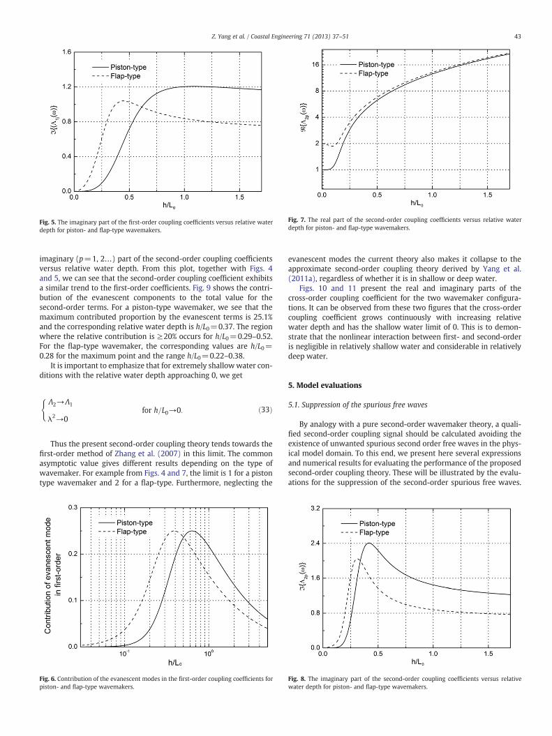
Fig. 7. The real part of the second-order coupling coefficients versus relative waterdepth for piston- and flap-type wavemakers.

Fig. 5. The imaginary part of the first-order coupling coefficients versus relative waterdepth for piston- and flap-type wavemakers.

43Z. Yang et al. / Coastal Engineering 71 (2013) 37–51

imaginary (p=1, 2…) part of the second-order coupling coefficientsversus relative water depth. From this plot, together with Figs. 4and 5, we can see that the second-order coupling coefficient exhibitsa similar trend to the first-order coefficients. Fig. 9 shows the contri-bution of the evanescent components to the total value for thesecond-order terms. For a piston-type wavemaker, we see that themaximum contributed proportion by the evanescent terms is 25.1%and the corresponding relative water depth is h/L0=0.37. The regionwhere the relative contribution is ≥20% occurs for h/L0=0.29–0.52.For the flap-type wavemaker, the corresponding values are h/L0=0.28 for the maximum point and the range h/L0=0.22–0.38.

It is important to emphasize that for extremely shallowwater con-ditions with the relative water depth approaching 0, we get

Λ2→Λ1

λ2→0for h=L0→0:

(ð33Þ

Thus the present second-order coupling theory tends towards thefirst-order method of Zhang et al. (2007) in this limit. The commonasymptotic value gives different results depending on the type ofwavemaker. For example from Figs. 4 and 7, the limit is 1 for a pistontype wavemaker and 2 for a flap-type. Furthermore, neglecting the

Fig. 6. Contribution of the evanescent modes in the first-order coupling coefficients forpiston- and flap-type wavemakers.

evanescent modes the current theory also makes it collapse to theapproximate second-order coupling theory derived by Yang et al.(2011a), regardless of whether it is in shallow or deep water.

Figs. 10 and 11 present the real and imaginary parts of thecross-order coupling coefficient for the two wavemaker configura-tions. It can be observed from these two figures that the cross-ordercoupling coefficient grows continuously with increasing relativewater depth and has the shallow water limit of 0. This is to demon-strate that the nonlinear interaction between first- and second-orderis negligible in relatively shallow water and considerable in relativelydeep water.

5. Model evaluations

5.1. Suppression of the spurious free waves

By analogy with a pure second-order wavemaker theory, a quali-fied second-order coupling signal should be calculated avoiding theexistence of unwanted spurious second order free waves in the phys-ical model domain. To this end, we present here several expressionsand numerical results for evaluating the performance of the proposedsecond-order coupling theory. These will be illustrated by the evalu-ations for the suppression of the second-order spurious free waves.

Fig. 8. The imaginary part of the second-order coupling coefficients versus relativewater depth for piston- and flap-type wavemakers.

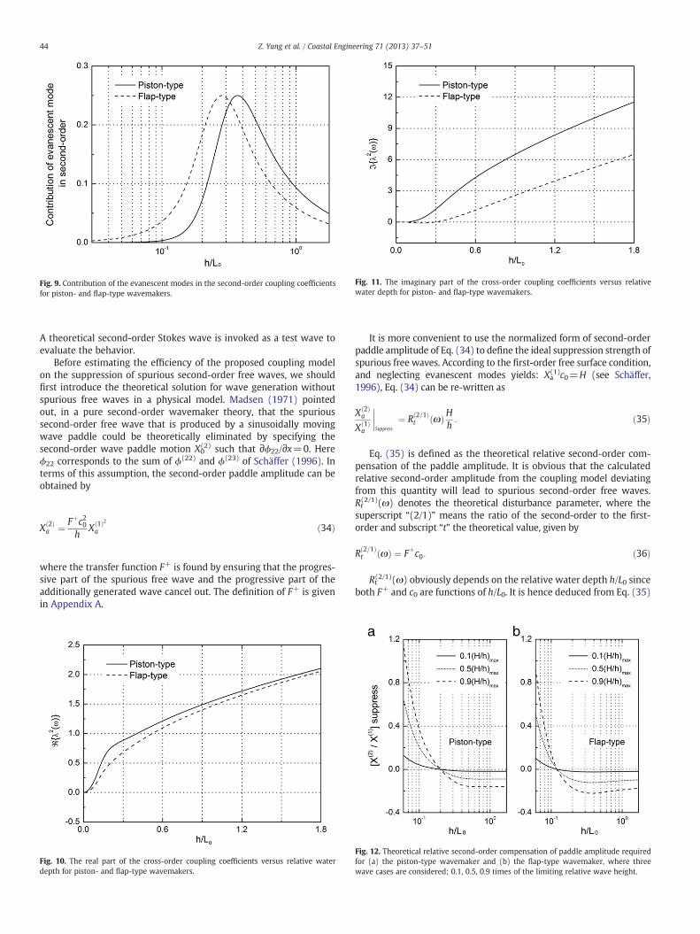
Fig. 11. The imaginary part of the cross-order coupling coefficients versus relativewater depth for piston- and flap-type wavemakers.

Fig. 9. Contribution of the evanescent modes in the second-order coupling coefficientsfor piston- and flap-type wavemakers.

44 Z. Yang et al. / Coastal Engineering 71 (2013) 37–51

A theoretical second-order Stokes wave is invoked as a test wave toevaluate the behavior.

Before estimating the efficiency of the proposed coupling modelon the suppression of spurious second-order free waves, we shouldfirst introduce the theoretical solution for wave generation withoutspurious free waves in a physical model. Madsen (1971) pointedout, in a pure second-order wavemaker theory, that the spurioussecond-order free wave that is produced by a sinusoidally movingwave paddle could be theoretically eliminated by specifying thesecond-order wave paddle motion X0

(2) such that ∂ϕ22/∂x=0. Hereϕ22 corresponds to the sum of ϕ(22) and ϕ(23) of Schäffer (1996). Interms of this assumption, the second-order paddle amplitude can beobtained by

X 2ð Þa ¼ Fþc20

hX 1ð Þ2a ð34Þ

where the transfer function F+ is found by ensuring that the progres-sive part of the spurious free wave and the progressive part of theadditionally generated wave cancel out. The definition of F+ is givenin Appendix A.

Fig. 10. The real part of the cross-order coupling coefficients versus relative waterdepth for piston- and flap-type wavemakers.

It is more convenient to use the normalized form of second-orderpaddle amplitude of Eq. (34) to define the ideal suppression strength ofspurious free waves. According to the first-order free surface condition,and neglecting evanescent modes yields: Xa

(1)c0=H (see Schäffer,1996), Eq. (34) can be re-written as

X 2ð Þa

X 1ð Þa Suppress

¼ R 2=1ð Þt ωð ÞH

h:

���� ð35Þ

Eq. (35) is defined as the theoretical relative second-order com-pensation of the paddle amplitude. It is obvious that the calculatedrelative second-order amplitude from the coupling model deviatingfrom this quantity will lead to spurious second-order free waves.Rt(2/1)(ω) denotes the theoretical disturbance parameter, where the

superscript “(2/1)” means the ratio of the second-order to the first-order and subscript “t” the theoretical value, given by

R 2=1ð Þt ωð Þ ¼ Fþc0: ð36Þ

Rt(2/1)(ω) obviously depends on the relative water depth h/L0 since

both F+ and c0 are functions of h/L0. It is hence deduced from Eq. (35)

Fig. 12. Theoretical relative second-order compensation of paddle amplitude requiredfor (a) the piston-type wavemaker and (b) the flap-type wavemaker, where threewave cases are considered; 0.1, 0.5, 0.9 times of the limiting relative wave height.

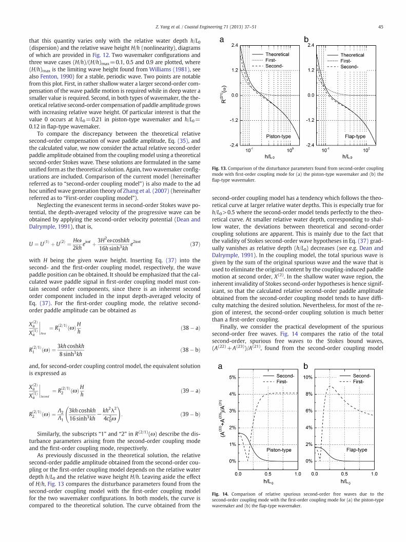
Fig. 13. Comparison of the disturbance parameters found from second-order couplingmode with first-order coupling mode for (a) the piston-type wavemaker and (b) theflap-type wavemaker.

Fig. 14. Comparison of relative spurious second-order free waves due to thesecond-order coupling mode with the first-order coupling mode for (a) the piston-typewavemaker and (b) the flap-type wavemaker.

45Z. Yang et al. / Coastal Engineering 71 (2013) 37–51

that this quantity varies only with the relative water depth h/L0(dispersion) and the relative wave height H/h (nonlinearity), diagramsof which are provided in Fig. 12. Two wavemaker configurations andthree wave cases (H/h)/(H/h)max=0.1, 0.5 and 0.9 are plotted, where(H/h)max is the limiting wave height found from Williams (1981), seealso Fenton, 1990) for a stable, periodic wave. Two points are notablefrom this plot. First, in rather shallowwater a larger second-order com-pensation of the wave paddle motion is required while in deep water asmaller value is required. Second, in both types of wavemaker, the the-oretical relative second-order compensation of paddle amplitude growswith increasing relative wave height. Of particular interest is that thevalue 0 occurs at h/L0=0.21 in piston-type wavemaker and h/L0=0.12 in flap-type wavemaker.

To compare the discrepancy between the theoretical relativesecond-order compensation of wave paddle amplitude, Eq. (35), andthe calculated value, we now consider the actual relative second-orderpaddle amplitude obtained from the couplingmodel using a theoreticalsecond-order Stokes wave. These solutions are formulated in the sameunified form as the theoretical solution. Again, twowavemaker config-urations are included. Comparison of the current model (hereinafterreferred as to “second-order coupling model”) is also made to the adhoc unifiedwave generation theory of Zhang et al. (2007) (hereinafterreferred as to “First-order coupling model”).

Neglecting the evanescent terms in second-order Stokes wave po-tential, the depth-averaged velocity of the progressive wave can beobtained by applying the second-order velocity potential (Dean andDalrymple, 1991), that is,

U ¼ U 1ð Þ þ U 2ð Þ ¼ Hω2kh

eiωt þ 3H2ω coshkh16h sinh3kh

e2iωt ð37Þ

with H being the given wave height. Inserting Eq. (37) into thesecond- and the first-order coupling model, respectively, the wavepaddle position can be obtained. It should be emphasized that the cal-culated wave paddle signal in first-order coupling model must con-tain second order components, since there is an inherent secondorder component included in the input depth-averaged velocity ofEq. (37). For the first-order coupling mode, the relative second-order paddle amplitude can be obtained as

X 2ð Þa

X 1ð Þa First

¼ R 2=1ð Þ1 ωð ÞH

h

���� ð38� aÞ

R 2=1ð Þ1 ωð Þ ¼ 3kh coshkh

8 sinh3khð38� bÞ

and, for second-order coupling control model, the equivalent solutionis expressed as

X 2ð Þa

X 1ð Þa Second

¼ R 2=1ð Þ2 ωð ÞH

h

���� ð39� aÞ

R 2=1ð Þ2 ωð Þ ¼ Λ2

Λ1

3kh coshkh16 sinh3kh

− kh2λ2

4c20ω

!: ð39� bÞ

Similarly, the subscripts “1” and “2” in R(2/1)(ω) describe the dis-turbance parameters arising from the second-order coupling modeand the first-order coupling mode, respectively.

As previously discussed in the theoretical solution, the relativesecond-order paddle amplitude obtained from the second-order cou-pling or the first-order coupling model depends on the relative waterdepth h/L0 and the relative wave height H/h. Leaving aside the effectof H/h, Fig. 13 compares the disturbance parameters found from thesecond-order coupling model with the first-order coupling modelfor the two wavemaker configurations. In both models, the curve iscompared to the theoretical solution. The curve obtained from the

second-order coupling model has a tendency which follows the theo-retical curve at larger relative water depths. This is especially true forh/L0>0.5 where the second-order model tends perfectly to the theo-retical curve. At smaller relative water depth, corresponding to shal-low water, the deviations between theoretical and second-ordercoupling solutions are apparent. This is mainly due to the fact thatthe validity of Stokes second-order wave hypotheses in Eq. (37) grad-ually vanishes as relative depth (h/L0) decreases (see e.g. Dean andDalrymple, 1991). In the coupling model, the total spurious wave isgiven by the sum of the original spurious wave and the wave that isused to eliminate the original content by the coupling-induced paddlemotion at second order, X(2). In the shallow water wave region, theinherent invalidity of Stokes second-order hypotheses is hence signif-icant, so that the calculated relative second-order paddle amplitudeobtained from the second-order coupling model tends to have diffi-culty matching the desired solution. Nevertheless, for most of the re-gion of interest, the second-order coupling solution is much betterthan a first-order coupling.

Finally, we consider the practical development of the spurioussecond-order free waves. Fig. 14 compares the ratio of the totalsecond-order, spurious free waves to the Stokes bound waves,(A(22)+A(23))/A(21), found from the second-order coupling model

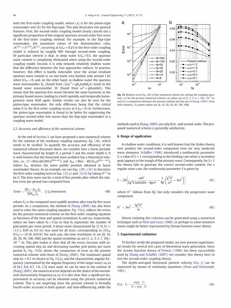
Fig. 15. Relative error Eq. (40) of the numerical scheme for solving the coupling equa-tion; (a) for the present numerical scheme, Δx values are at [1, 2, 3, 5, 7, 10]×10-2 m;and (b) a comparison between the present method and the one of Zhang (2005) (lineswith markers), Nt points values are [8, 10, 20, 30, 50, 100, 500].

46 Z. Yang et al. / Coastal Engineering 71 (2013) 37–51

with the first-order coupling model, where (a) is for the piston-typewavemaker and (b) for the flap-type. This plot illustrates two generalfeatures. First, the second-order coupling model clearly cancels out asignificant proportion of the original spurious second order free waveof the first-order coupling method. For example, in the flap-typewavemaker, the maximum values of the dimensionless ratio,(A(22)+A(23))/A(21), occurring at h/L0=0.25 in the first-order couplingmodel is reduced by roughly 90% through second-order coupling.Of particular interest is that, in deep water h/L0>0.5, the spuriouswave content is completely eliminated when using the second-ordercoupling model. Second, it is only towards relatively shallow waterthat the difference between the two approaches reduces. In practice,however, this effect is hardly noticeable since the actual resultantspurious wave content is, on one hand, very limited, only around 1.6%when h/L0→0, and, on the other hand, in shallow water the spuriouswave wavenumber Kp (found from (2ω)2=gKptanhKph) tends to thebound wave wavenumber 2k (found from ω2=gktanhkh). Thismeans that the spurious free waves become the same harmonic as theprimary boundwaves, leading to a both spatially and temporally homo-geneous wave field again. Similar results can also be seen for thepiston-type wavemaker, the only difference being that the criticalvalue 0 in the first-order coupling occurs at h/L0=0.14. Furthermore,the piston-type wavemaker is found to be better for suppressing thespurious second-order free waves than the flap-type wavemaker in acoupling wave model.

5.2. Accuracy and efficiency of the numerical scheme

At the end of Section 3, we have proposed a new numerical schemefor the solution of the nonlinear coupling equations, Eq. (28), whichneeds to be verified. To quantify the accuracy and efficiency of thenumerical scheme discussed above, we consider here a linear periodicwave characterized by height H, a period T and the water depth h. Itis well-known that the linearized wave problem has a theoretical solu-tion, i.e., U=Re{(ωH/2kh)ei(kx-ωt)} and Xlin.=Re{(−iH/2c0)ei(kx−ωt)},where Xlin. denotes the wave paddle position obtained in linearwavemaker theory. As an example, we use Eqs. (29)–(32) to discretizethe first-order coupling term in Eqs. (12-a) and (12-b) by taking U(1) tobe U. The tests were run for a total of five periods after which the rela-tive error per period was computed from

Error ¼ ‖X5−Xlin:‖25‖Xlin:‖2

; ‖⋅‖2≡twonorm ð40Þ

where X5 is the computed wave paddle position after exactly five waveperiods. As a comparison, the method of Zhang (2005) has also beenused to solve the same coupling equation. Fig. 15(a) collects the errorsfor the present numerical scheme on the first-order coupling equationas functions of the time and spatial resolutions Nt and Δx, respectively,where we have taken Nt=T/Δt so that Nt represents the number ofgrid points per wave period. A linear wave characterized by (T, H, h)=(1.5 s, 0.05 m, 0.5 m) was used for all tests, corresponding to (h/L0,H/L0)=(0.18, 0.018). For each case, the time resolutions Nt are [8, 10,20, 30, 50, 100, 500] and the spatial resolution Δx are [1, 2, 3, 5, 7, 10]×10−2 m. This plot makes it clear that all the errors increase with in-creasing spatial step Δx and decreasing number grid points per waveperiod Nt. Fig. 15(b) shows the comparison of error on the presentnumerical scheme with those of Zhang (2005). The maximum spatialstep Δx=0.1 m chosen in Fig. 15(a), and the characteristic angular fre-quency (normalized by the angular frequency of the target wave) ωc/ωof [0.1, 0.4, 0.7, 1.0, 1.2] were used. As can be seen in the scheme ofZhang (2005), the numerical error depends on the choice of the normal-ized characteristic frequency ωc/ω. It is also clear that, a significant im-provement in accuracy can be obtained using the present numericalscheme. This is not surprising since the present scheme is formallyfourth-order accurate in both spatial- and time-differencing, while the

methods used in Zhang (2005) are only first- and second-order. The pro-posed numerical scheme is generally satisfactory.

6. Range of application

In shallow water conditions, it is well known that the Stokes theoryover predicts the second-order component even for very moderatewave steepness. Schäffer (1996) introduced a nonlinearity parameterS; a value of S=1 corresponding to the limiting case when a secondarypeak appears in the trough of the primary wave. Consequently, for S>1the theory fails to generate the correct second-order content. For aregular wave case, the nonlinearity parameter S is given by

S ¼ 2HωHþ

2g2k tanh2kh−4gω2 −14g

g2k2

ω2 −3ω2

!���������� ð41Þ

where H+ follows from Hjk+ but only considers the progressive wave

component

Hþ ¼ 3ω3−3g2k2

ω: ð42Þ

Waves violating this criterion can be generated using a numericaltechnique such as Flick and Guza (1980), or perhaps in some instanceswaves might be better represented by Stream function wave theory.

7. Experimental validation

To further verify the proposed model, we now present experimen-tal results for several test cases of theoretical wave generation. Sincethe stream function theory of Fenton (1988) has been successfullyused by Zhang and Schäffer (2007) we consider this theory here totest the second-order coupling theory.

The depth-averaged horizontal particle velocity U(x, t) can beexpressed by means of continuity equations (Dean and Dalrymple,1991)

U x; tð Þ ¼ cη x; tð Þhþ η x; tð Þ ð43Þ

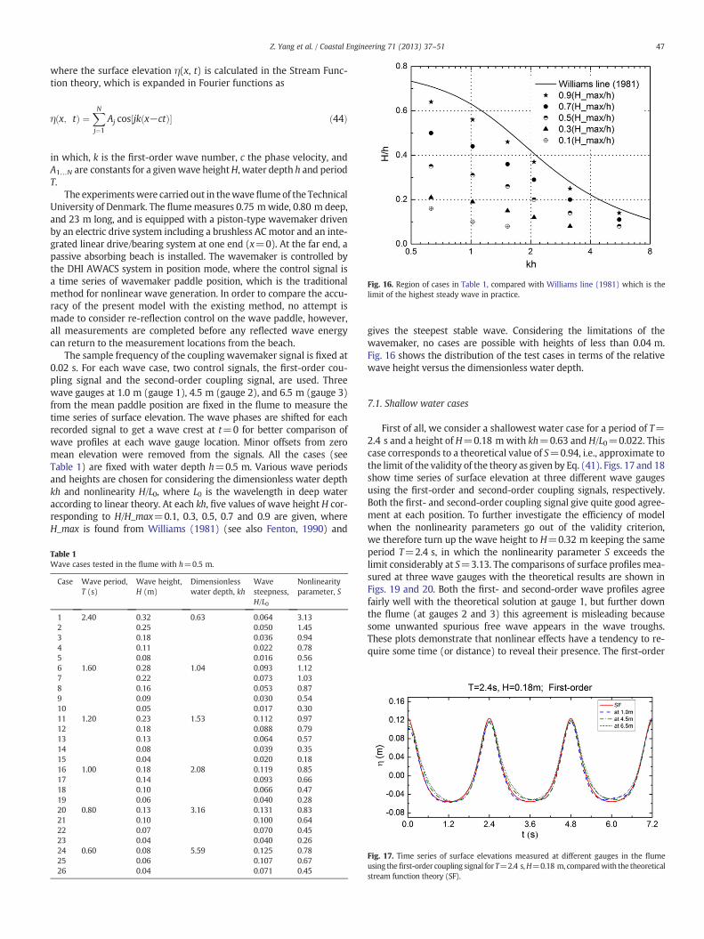
Fig. 16. Region of cases in Table 1, compared with Williams line (1981) which is thelimit of the highest steady wave in practice.

47Z. Yang et al. / Coastal Engineering 71 (2013) 37–51

where the surface elevation η(x, t) is calculated in the Stream Func-tion theory, which is expanded in Fourier functions as

η x; tð Þ ¼XNj¼1

Aj cos jk x−ctð Þ½ � ð44Þ

in which, k is the first-order wave number, c the phase velocity, andA1…N are constants for a givenwave heightH, water depth h and periodT.

The experimentswere carried out in thewave flumeof the TechnicalUniversity of Denmark. The flumemeasures 0.75 mwide, 0.80 m deep,and 23 m long, and is equipped with a piston-type wavemaker drivenby an electric drive system including a brushless AC motor and an inte-grated linear drive/bearing system at one end (x=0). At the far end, apassive absorbing beach is installed. The wavemaker is controlled bythe DHI AWACS system in position mode, where the control signal isa time series of wavemaker paddle position, which is the traditionalmethod for nonlinear wave generation. In order to compare the accu-racy of the present model with the existing method, no attempt ismade to consider re-reflection control on the wave paddle, however,all measurements are completed before any reflected wave energycan return to the measurement locations from the beach.

The sample frequency of the coupling wavemaker signal is fixed at0.02 s. For each wave case, two control signals, the first-order cou-pling signal and the second-order coupling signal, are used. Threewave gauges at 1.0 m (gauge 1), 4.5 m (gauge 2), and 6.5 m (gauge 3)from the mean paddle position are fixed in the flume to measure thetime series of surface elevation. The wave phases are shifted for eachrecorded signal to get a wave crest at t=0 for better comparison ofwave profiles at each wave gauge location. Minor offsets from zeromean elevation were removed from the signals. All the cases (seeTable 1) are fixed with water depth h=0.5 m. Various wave periodsand heights are chosen for considering the dimensionless water depthkh and nonlinearity H/L0, where L0 is the wavelength in deep wateraccording to linear theory. At each kh, five values of wave height H cor-responding to H/H_max=0.1, 0.3, 0.5, 0.7 and 0.9 are given, whereH_max is found from Williams (1981) (see also Fenton, 1990) and

Table 1Wave cases tested in the flume with h=0.5 m.

Case Wave period,T (s)

Wave height,H (m)

Dimensionlesswater depth, kh

Wavesteepness,H/L0

Nonlinearityparameter, S

1 2.40 0.32 0.63 0.064 3.132 0.25 0.050 1.453 0.18 0.036 0.944 0.11 0.022 0.785 0.08 0.016 0.566 1.60 0.28 1.04 0.093 1.127 0.22 0.073 1.038 0.16 0.053 0.879 0.09 0.030 0.5410 0.05 0.017 0.3011 1.20 0.23 1.53 0.112 0.9712 0.18 0.088 0.7913 0.13 0.064 0.5714 0.08 0.039 0.3515 0.04 0.020 0.1816 1.00 0.18 2.08 0.119 0.8517 0.14 0.093 0.6618 0.10 0.066 0.4719 0.06 0.040 0.2820 0.80 0.13 3.16 0.131 0.8321 0.10 0.100 0.6422 0.07 0.070 0.4523 0.04 0.040 0.2624 0.60 0.08 5.59 0.125 0.7825 0.06 0.107 0.6726 0.04 0.071 0.45

gives the steepest stable wave. Considering the limitations of thewavemaker, no cases are possible with heights of less than 0.04 m.Fig. 16 shows the distribution of the test cases in terms of the relativewave height versus the dimensionless water depth.

7.1. Shallow water cases

First of all, we consider a shallowest water case for a period of T=2.4 s and a height of H=0.18 mwith kh=0.63 and H/L0=0.022. Thiscase corresponds to a theoretical value of S=0.94, i.e., approximate tothe limit of the validity of the theory as given by Eq. (41). Figs. 17 and 18show time series of surface elevation at three different wave gaugesusing the first-order and second-order coupling signals, respectively.Both the first- and second-order coupling signal give quite good agree-ment at each position. To further investigate the efficiency of modelwhen the nonlinearity parameters go out of the validity criterion,we therefore turn up the wave height to H=0.32 m keeping the sameperiod T=2.4 s, in which the nonlinearity parameter S exceeds thelimit considerably at S=3.13. The comparisons of surface profiles mea-sured at three wave gauges with the theoretical results are shown inFigs. 19 and 20. Both the first- and second-order wave profiles agreefairly well with the theoretical solution at gauge 1, but further downthe flume (at gauges 2 and 3) this agreement is misleading becausesome unwanted spurious free wave appears in the wave troughs.These plots demonstrate that nonlinear effects have a tendency to re-quire some time (or distance) to reveal their presence. The first-order

Fig. 17. Time series of surface elevations measured at different gauges in the flumeusing thefirst-order coupling signal for T=2.4 s,H=0.18 m, comparedwith the theoreticalstream function theory (SF).

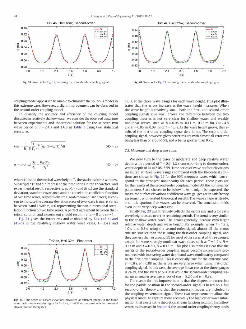
Fig. 18. Same as for Fig. 17, but using the second-order coupling signal. Fig. 20. Same as for Fig. 19, but using the second-order coupling signal.

48 Z. Yang et al. / Coastal Engineering 71 (2013) 37–51

couplingmodel appears to be unable to eliminate the spuriousmodes inthis extreme case. However, a slight improvement can be observed inthe second-order coupling model.

To quantify the accuracy and efficiency of the coupling modeldiscussed in relatively shallowwater,we consider the observeddeparturebetween experiments and theoretical solution for the selected twowave period of T=2.4 s and 1.6 s in Table 1 using two statisticalerrors, i.e.

rms ¼ 1HT

ffiffiffiffiffiffiffiffiffiffiffiffiffiffiffiffiffiffiffiffiffiffiffiffiffiffiffiffiffiffiffiffiffiffiffiffiffiffiffiffiffiffiffiffiffiffiffiffiffiffi1Tn

∫Tn0 ηT tð Þ−ηP tð Þ� �2dt

sð45� aÞ

α ¼ ρTP τ0ð ÞσP

σT¼ RTP τ0ð Þ

σT2 ð45� bÞ

whereHT is the theoretical wave height, Tn the statistical timewindow.Subscripts “T” and “P” represent the time series in the theoretical andexperimental result, respectively. σ, ρ(τ0) and R(τ0) are the standarddeviation, standard covariance and the correlation coefficient functionof two time series, respectively. rms (root-mean-square errors) is cho-sen to indicate the average deviation error of twowave trains. α variesbetween 0 and 1 with τ0=0 representing the non-dimensional corre-lation function of two time series. A perfect agreement between theo-retical solution and experiment should result in rms→0 and α→1.

Fig. 21 gives the errors rms and α obtained by Eqs. (45-a) and(45-b) in the relatively shallow water wave cases, T=2.4 s and

Fig. 19. Time series of surface elevations measured at different gauges in the flumeusing thefirst-order coupling signal for T=2.4 s,H=0.32 m, comparedwith the theoreticalstream function theory (SF).

1.6 s, at the three wave gauges for each wave height. This plot illus-trates that the errors increase as the wave height increases. Whenthe wave height is relatively small, both the first- and second-ordercoupling signals give small errors. The difference between the twocoupling theories is not very clear for shallow water and weaklynonlinear waves, such as H=0.08 m, 0.11 m, 0.25 m for T=2.4 sand H=0.05 m, 0.09 m for T=1.6 s. As the wave height grows, the re-sults of the first-order coupling signal deteriorate. The second-ordercoupling signal, however, gives better results with almost all error rmsbeing less than or around 5%, and α being greater than 0.75.

7.2. Moderate and deep water cases

We now turn to the cases of moderate and deep relative waterdepth with a period of T=0.6–1.2 s corresponding to dimensionlesswater depth of kh=2.08–5.59. Time series of wave surface elevationsmeasured at three wave gauges compared with the theoretical solu-tions are shown in Fig. 22 for the 90% steepness cases, which corre-spond to the strongest nonlinearity for each period. These plots arefor the results of the second-order coupling model. All the nonlinearityparameters S are chosen to be below 1. As it might be expected, themeasured surface elevations at differentwave gauges are in satisfactoryagreement with related theoretical results. The wave shape is steady,and little spurious free waves can be observed. The conclusion holdseven in the very deep water case.

Finally, Fig. 23 quantitatively collects the errors rms and α for eachwave height tested over the remaining periods. The trend is very similarto the shallow water cases. The errors generally increase with largerrelative water depth and wave height. For example, when T=1.2 s,1.0 s, and 0.8 s, using the second-order signal, almost all the errorsrms are smaller than those using the first-order coupling signal, andthey are less than or around 5% for most of the cases at all three gauges,except for some strongly nonlinear wave cases such as T=1.2 s, H=0.23 m and T=0.8 s, H=0.13 m. This plot also makes it clear that themerits of the second-order coupling signal become increasingly pro-nounced with increasing water depth and wave nonlinearity comparedto the first-order coupling. This is especially true for the extreme case,T=0.6 s, H=0.08 m, the errors are very large when using first-ordercoupling signal. In this case, the average linear rms at the three gaugesis 24.2%, and the average α is 0.58 while the second-order coupling sig-nal gives smaller average errors of rms=9.2% and α=0.88.

The reason for this improvement is that the dispersion correctionfor the paddle position in the second-order signal is based on a fullsecond-order theory and that the evanescent modes are included inthe coupling wavemaker signal. These two improvements allow thephysical model to capture more accurately the high order wave infor-mation that exists in the theoretical stream function solution. In shallowwater, as discussed in Section 4, the second-order coupling theory tends

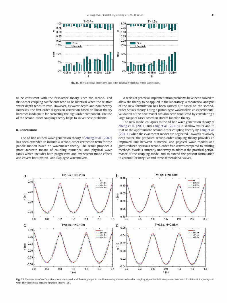
Fig. 21. The statistical errors rms and α for relatively shallow water wave cases.

49Z. Yang et al. / Coastal Engineering 71 (2013) 37–51

to be consistent with the first-order theory since the second- andfirst-order coupling coefficients tend to be identical when the relativewater depth tends to zero. However, as water depth and nonlinearityincreases, the first-order dispersion correction based on linear theorybecomes inadequate for correcting the high order component. The useof the second-order coupling theory helps to solve these problems.

8. Conclusions

The ad hoc unified wave generation theory of Zhang et al. (2007)has been extended to include a second-order correction term for thepaddle motion based on wavemaker theory. The result provides amore accurate means of coupling numerical and physical wavetanks which includes both progressive and evanescent mode effectsand covers both piston- and flap-type wavemakers.

Fig. 22. Time series of surface elevations measured at different gauges in the flume using thwith the theoretical stream function theory (SF).

A series of practical implementation problems have been solved toallow the theory to be applied in the laboratory. A theoretical analysisof the new formulation has been carried out based on the second-order Stokes theory. Using a piston-type wavemaker, an experimentalvalidation of the new model has also been conducted by considering alarge range of cases based on stream function theory.

The new model collapses to the ad hoc wave generation theory ofZhang et al. (2007) and Yang et al. (2011b) in shallow water and tothat of the approximate second-order coupling theory by Yang et al.(2011a) when the evanescent modes are neglected. Towards relativelydeep water, the proposed second-order coupling theory provides animproved link between numerical and physical wave models andgives reduced spurious second-order free waves compared to existingmethods. Work is currently underway to address the practical perfor-mance of the coupling model and to extend the present formulationto account for irregular and three-dimensional waves.

e second-order coupling signal for 90% steepness cases with T=0.6 s–1.2 s, compared

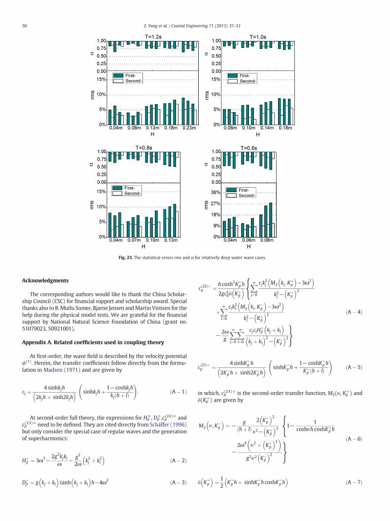
Fig. 23. The statistical errors rms and α for relatively deep water wave cases.

50 Z. Yang et al. / Coastal Engineering 71 (2013) 37–51

Acknowledgments

The corresponding authors would like to thank the China Scholar-ship Council (CSC) for financial support and scholarship award. Specialthanks also to B. Mutlu Sumer, Bjarne Jensen andMartin Vistisen for thehelp during the physical model tests. We are grateful for the financialsupport by National Natural Science Foundation of China (grant no.51079023, 50921001).

Appendix A. Related coefficients used in coupling theory

At first-order, the wave field is described by the velocity potentialϕ(1). Herein, the transfer coefficients follow directly from the formu-lation in Madsen (1971) and are given by

cj ¼4 sinhkjh

2kjhþ sinh2kjh� � sinhkjhþ 1− coshkjh

kj hþ lð Þ

!: ðA� 1Þ

At second-order full theory, the expressions for Hjl+, Djl

+,cp(22)+ andcp(23)+ need to be defined. They are cited directly from Schäffer (1996)but only consider the special case of regular waves and the generationof superharmonics:

Hþjl ¼ 3ω3−

2g2kjklω

− g2

2ωk2j þ k2l� �

ðA� 2Þ

Dþjl ¼ g kj þ kl

� �tanh kj þ kl

� �h−4ω2 ðA� 3Þ

c 22ð Þþp ¼ h cosh2Kþ

p h

2gc20δ Kþp

� �fX∞j¼0

cjk2j M2 kj;K

þp

� �−3ω2

� �k2j − Kþ

p

� �2

þX∞l¼0

clk2l M2 kl;K

þp

� �−3ω2

� �k2l − Kþ

p

� �2

−2ωg

X∞j¼0

X∞l¼0

cjclHþjl kj þ kl� �

kj þ kl� �2− Kþ

p

� �2gðA� 4Þ

c 23ð Þþp ¼ 4 sinhKþ

p h

2Kþp hþ sinh2Kþ

p h� � sinhKþ

p hþ 1− coshKþp h

Kþp hþ lð Þ

!ðA� 5Þ

in which, cp(23)+ is the second-order transfer function, M2(κ, Kp+) and

δ(Kp+) are given by

M2 κ ;Kþp

� �¼ − g

hþ lð Þ2 Kþ

p

� �2κ2− Kþ

p

� �2 f1− 1coshκh coshKþ

p h

−2ω4 κ2 þ Kþ

p

� �2�

g2κ2 Kþp

� �2 g ðA� 6Þ

δ Kþp

� �¼ 1

2Kþp hþ sinhKþ

p h coshKþp h

� �ðA� 7Þ

51Z. Yang et al. / Coastal Engineering 71 (2013) 37–51

where Kp+ is second-order wave number, obtained by

2ωð Þ2 ¼ gKþp tanhKþ

p h ðA� 8Þ

which is the dispersion equation generalized to the second-ordercomplex numbers. The transfer function F+ found by Schäffer (1996)is described as

Fþ ¼ − c 22ð Þþ0

c 23ð Þþ0

ðA� 9Þ

where the subscript “0” denotes the progressive-wave components(p→0).

References

Dean, R.G., Dalrymple, R.A., 1991. Water Wave Mechanics for Engineering and Scientific.World Scientific, Singapore, pp. 295–324.

Fenton, J.D., 1988. The numerical solution of steady water wave problems. Computersand Geosciences 14 (3), 357–368.

Fenton, J.D., 1990. Nonlinear wave theories. In: Le Mehaute, B., Hanes, D.M. (Eds.), TheSea, pp. 3–25.

Flick, R.E., Guza, R.T., 1980. Paddle generated waves in laboratory channels. Journal ofWaterway, Port, Coastal, and Ocean Engineering 106 (WW1), 79–97.

Fontanet, P., 1961. Théorie de la génération de la home cylindrique parun batteur plan.La Huille Blanche 16, 3–31 ((part 1) and 174–196 (part 2)).

Hudspeth, R.T., Sulisz, W., 1991. Stokes drift in two-dimensional wave flumes. Journalof Fluid Mechanics 230, 209–229.

Madsen, O.S., 1971. On the generation of long waves. Journal of Geophysical Research76, 8672–8683.

Ottesen-Hansen, N.E., Sand, S.E., Lundgren, H., Sorensen, T., Gravesen, H., 1980. Correctreproduction of long group induced waves. Proceedings of the 17th Coastal Engi-neering Conference, Sydney, Australia, pp. 784–800.

Sand, S.E., 1982. Long wave problems in laboratory models. Journal of Waterway, Port,Coastal, and Ocean Engineering 108 (WW4), 492–503.

Sand, S.E., Donslund, B., 1985. Influence of the wave board type on bounded longwaves. Journal of Hydraulic Research 23, 147–163.

Schäffer, H.A., 1996. Second-order wavemaker theory for irregular waves. Ocean Engi-neering 23, 47–88.

Sulisz, W., Hudspeth, R.T., 1993. Complete second-order solution for water waves gen-erated in wave flumes. Journal of Fluids and Structures 7, 253–268.

Synolakis, C.E., 1990. Generation of long waves in laboratory. Journal of Waterway,Port, Coastal, and Ocean Engineering 116 (2), 252–266.

Williams, J.M., 1981. Limiting gravity waves in water of finite depth. PhilosophicalTransactions of the Royal Society of London A 302, 139–188.

Yang, Z.W., Liu, S.X., Chang, J., Li, J.X., Sun, Z.B., 2011a. On the approximate second-order coupling theory of numerical and physical wave model in flumes. Proceed-ings of the 21th International Offshore and Polar Engineering Conference, Maui,Hawaii, USA, June 19–24, 2011.

Yang, Z.W., Liu, S.X., Li, J.X., Sun, Z.B., 2011b. Coupling of numerical and physical modelfor simulation of wave propagation. Journal of Hydrodynamics, Series A 26 (3),296–306.

Zhang, H., 2005. A deterministic combination of numerical and physical models forcoastal waves. Ph.D. thesis, Technical University of Denmark, pp. 33–68.

Zhang, H., Schäffer, H.A., 2004. Waves in numerical and physical wave flumes — adeterministic combination. Proceedings of the 29th International Conference onCoastal Engineering, Lisbon, Portugal, September 2004.

Zhang, H., Schäffer, H.A., 2005. Waves in numerical and physical wave basins— a deter-ministic combination. Proceedings of Waves 2005, Madrid, Spain, July 2005.

Zhang, H., Schäffer, H.A., 2007. Approximate stream function wavemaker theory forhighly non-linear waves in wave flumes. Ocean Engineering 34, 1290–1302.

Zhang, H., Schäffer, H.A., Jakobsen, K.P., 2007. Deterministic combination of numericaland physical coastal wave models. Coastal Engineering 54, 171–186.