Sediment transport: Physical modelling of flocculation

Environmetrics; 1990; l(2): 195-209 @Enuironmetrics Press, Canada

Sediment Transport: Physical Modelling of Flocculation

U. J. Jeffrey'

ABSTRACT

A study is made of the behaviour of cohesive sediment in turbulent flowfields, such as are found in strongly tidal river estuaries. A model is developed which incorporates the fact that cohesive sediments, usually clays, consist of particles which can flocculate because of the electrical charges on them. During the cycle of erosion and deposition that occurs in tidal estuaries, the degree of flocculation changes. An equation is formulated for the evolution of the size distribution of the particle aggregates in suspension, taking into account the effect of turbulence both on the rates of flocculation and breakup. Solutions of this equation are obtained using an extension of the quasi-stationary approximation. The results are used to investigate the interpretation of the output of electro-optical turbidity meters. These are important sources of field measurements, but they require calibration before their data can be used for the testing and construction of sediment transport equations. It is shown that the transformation of turbidity-meter readings into density measurements requires statistical information about the sizes of the suspended aggregates. This can be calculated using the size distributions obtained from the model presented here, after they have been combined with an experimental determination of some empirical constants.

KEY WORDS: Sediment transport, estuaries, turbidity, aggregation, flocs, floc breakup, size distribution.

1. INTRODUCTION

The transport of sediment has a significant impact on the condition and uses of a river estuary. For example, much of the economic importance of

' Department of Applied Mathematics, The University of Western On- tario, London, Ontario, Canada N6A 5B9.

196 D. J. JEFFREY

estuaries is derived from their use for shipping, and if allowance is not made for sediment transport during the design of harbour facilities, the mainte- nance of navigational channels can become a major economic burden. It is possible to design a harbour that is practically free of dredging require- ments on a time scale of years, but in practice many badly designed harbours require annual, or more frequent , dredging. Another important reason for understanding sediment transport is the dispersal of pollutants, which can be greatly hindered by the properties of clay sediments. Clay particles typically expose, on their surfaces, faces of their underlying crystalline structure, and these faces present many adsorption sites for aqueous ions. The sites are responsible for creating the charges which are present on the particles, and also for the strong adsorption of other substances, such as heavy metal pollutants, in solution. Depending upon the transport patterns of the sediment, there can be either localized build-ups of pollutants or a general increase in the level of pollution throughout the estuary. In both of these examples, an important aspect is the fact that strongly tidal estuaries redistribute the same sediment over and over again. Although the rivers entering the estuary carry sediment, river load makes up only a small fraction of the total load suspended in the water at any particular time.

The study of sediment transport is complicated by two factors often present in the major estuaries of the world. The first of these is the nature of the fluid flow in the estuary. The tides of the sea can penetrate a consid- erablc distance inland, and are responsible for high levels of turbulence that dominate the flow fields in the estuary. In addition, turbulent mixing creates gradients of salinity from the fresh water of the river to the salt water of the sea arid determines the deposition patterns of the sediment. The second is the chemical nature of the sediment material which is commonly derived from clay. In suspension, clay is broken up into charged disk-shaped particles called platelets. The charges on the platelets are important for the transport of the sediment because the platelets cohere to an extent determined by the magnitude of the charges and by the local chemical constitution of the estuary water. Cohering clay particles that act as a unit are called a fioc. Floc sizes in turbulent flow are typically 30 to 100 pm in size, but this range varies considerably, because there is an equilibrium between the fluid forces tending to break the flocs apart, and the internal bonds in the floc keeping it together and attracting more platelets to it. If charges are not present on the particles, the sediment is referred to as non-cohesive and has quite different properties from cohesive sediment.

Any model of sediment transport must take into account the settling of the flocs under gravity. If we model a floc as a spherical particle, its rate of fall through the water is given by Stokes’s law as 2a2(pf - p)g/9p, where pf is the density of the floc and p and p are the density and viscosity of the water. We see that the settling velocity increases with particle size; this is because the fluid drag on small objects increases only linearly with radius

MODELLING OF FLOCCULATION 197

a, whereas the weight increases with the cube of the radius. The tendency to settle is counteracted by upward mixing due to fluid motion and thermal agitation (Brownian motion), and, as a rough estimate, particles must be greater than 100 pm in order to settle out of the water column. The calculation of settling velocity is further complicated by the fact that most recent investigations indicate that p is related to a through the fact that larger flocs are less dense than smaller ones, because the constituent clay particles are less perfectly packed. In addition we expect that the flocs will not be identical, but rather their sizes will be described by a distribution function which depends upon the fluid environment. In particular, the salinity and the strength of the turbulence are expected to play major roles in deter- mining the size distribution. An obvious example of this is the fact that sediment that has been carried great distances in the fresh water of a river will sediment upon meeting the salinity of an estuary. After that, sediment that has settled to the bottom of the estuary at slack tide will be picked up again during the next ebb or flood. We conclude, therefore, that information on the sizes of the flocs comprising the sediment is essential for any global transport model.

Experimental investigations of sediment transport have been based on measuring a density profile at some point in the estuary as a function of the vertical coordinate through the body of water. Typically, a ship is sailed to a measuring station and profiles are taken at different times during a tidal cycle; then the ship is sailed to another site and the profiling is repeated. The sort of information one would like, in addition to the concentration, is the local and instantaneous distribution of floc sizes and their densities. The measurement of these quantities has often been done by collecting water sam- ples and analysing them with a Coulter counter (Kranck 1981). This gives a low rate of data acquisition. More importantly, the measuring process alters the distribution of floc sizes in unknown ways. An electro-optical turbidity meter offers the advantages of frequent profiling of the water column, and of minimum disruption of the in situ conditions. It measures the opacity of the water, this being strongly affected by the quantity of sediment present. The relation between opacity and density is not a direct one, however, because the instrument responds more to the number and size of flocs present than it does to their density. Its full potential has therefore failed to be realised because of the lack of accurate calibrating information.

.

2. THE EQUATION GOVERNING THE SIZE DISTRIBUTION

The theoretical treatment of suspensions of flocs of different sizes starts with spherical objects. Flocs are indeed roughly spherical, but even if they were not, most theoretical treatments handle non-spherical particles by simply adding a shape factor in the equations for spherical particles. Consider

198 D. J . JEFFREY

a volume V containing Mp identical particles of diameter d. The particle number density N is defined to be M p / V and the volumetric particle concentration is CP = N7rd3/6. To take into account the fact that particles are not all of the same size, we generalize N to a distribution function. We first must choose a variable to characterize the size of a particle. Both particle volume v and particle diameter d can be used (Friedlander 1977); we use volume because it is conserved when two particles aggregate, but diameter is not. We further treat v as a continuous variable. In the case of clay flocs, this is reasonable, because a clay platelet is typically less than 1 pm in diameter and less than a tenth that in thickness, whereas a floc is about 30 pm in diameter. Let the number of flocs in the volume V that have volumes in thc range (v, v + dv) be given by

dMp = Vn(v) dv . (1)

Integrating over all possible floc volumes, we obtain

and thus N = - - n(v)dv 7-1- (3)

Although it is made clear in (1) that the number density of particles n is defined with respect to a size range (v,v + dv), there is no confusion if we refer loosely to particles of size v.

We derive an equation for n(v) by considering how the processes of aggregation and breakup alter the distribution. Such an approach has been used by Friedlander (1977) to derive a population equation for aerosols, but he coiisidered aggregation only and not breakup, so here we add the extra terms that are needed to the governing equation. Following on from the definitions above, we define P(v,v') as the rate at which particles of size v aggregate with those of size v'. That is, during the time interval (t, t+d t ) , the number of collisions that take place between particles of size v and particles of size v' and that create new flocs of size v + v' is

Althoiigh this statement simply says that volume is conserved during aggregation, a more elaborate theory might reconsider it. It is possible that the fluid forces on the floc will rearrange the constituent platelets to alter the geometry and apparent volume. Several authors have postulated some transformation like this, at least indirectly, because theories have been put forward in which the density of the floc decreases with increasing volume,


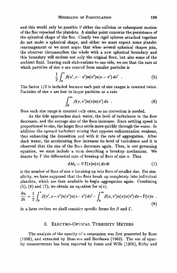
and this would only be possible if either the collision or subsequent motion of the floc repacked the platelets. A similar point concerns the persistence of the spherical shape of the floc. Clearly two rigid spheres attached together do not make a spherical shape, and either we must expect some platelet rearrangement or we must argue that when several spherical shapes join, the observer circumscribes the whole with a new spherical boundary and this boundary will enclose not only the original flocs, but also some of the ambient fluid. Leaving such elaborations to one side, we see that the rate at which particles of size v are created from smaller particles is

p(v', v - v')n(v')n(v - v') dv' . ; I' ( 5 )

The factor 1/2 is included because each pair of size ranges is counted twice. Particles of size v are lost to larger particles at a rate

brn P(v, v')n(v)n(v') dv . ( 6 )

Here each size range is counted only once, so no correction is needed. As the tide approaches slack water, the level of turbulence in the flow

decreases, and the average size of the flocs increases. Since settling speed is proportional to size, the larger flocs settle more quickly through the water. In addition the upward turbulent mixing that opposes sedimentation weakens, thus enhancing the deposition and with it the rate of aggregation. After slack water, the accelerating flow increases its level of turbulence and it is observed that the size of the flocs decreases again. Thus, in our governing equation, we must include a term describing a breakup mechanism. We denote by r the differential rate of breakup of flocs of size v. Thus

mb = vr(v)n(v) d v d t (7) is the number of flocs of size v breaking up into flocs of smaller size. For sim- plicity, we have supposed that t h e flocs break up completely into individual platelets, which are then available to begin aggregation again. Combining (5), (6) and (7), we obtain an eqiiation for n(v).

(8) In a later section we shall considor specific forms for p and I?.

3. ELECTRO-OPTICAL TURBIDITY METERS

The analysis of the opacity of a suspension was first presented by Rose (1950), and extended by Hom-ma and Horikawa (1963). The use of opacity measurements has been reported by Jones and Wills (1956), Kirby and

200 D. J. JEFFREY

Parker (1975), Basano, Ottonfello and Papa (1976) and other authors. Ap- plications to non-cohesive sediments have been more successful than those to cohesive ones, because the distribution of particle sizes in non-cohesive sediments can be obtained fairly easily and it does not change. On the other hand, applications to cohesive sediments have faced greater difficulties because of possible changes in the size distribution during the experiment.

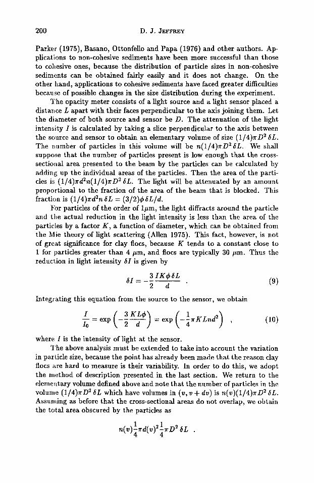
The opacity meter consists of a light source and a light sensor placed a distance L apart with their faces perpendicular to the axis joining them. Let the diameter of both source and sensor be D. The attenuation of the light intensity I is calculated by taking a slice perpendicular to the axis between the source and sensor to obtain an elementary volume of size (1/4)nD2 6L. The number of particles in this volume will be n(1/4)nD26L. We shall suppose that the number of particles present is low enough that the cross- sectional area presented to the beam by the particles can be calculated by adding up the individual areas of the particles. Then the area of the particles is (1/4)nd2n(1/4)nD2 6L. The light will be attenuated by an amount proportional to the fraction of the area of the beam that is blocked. This fraction is (1/4)nd2n 6L = (3/2)46L/d.

For particles of the order of lpm, the light diffracts around the particle and the actual reduction in the light intensity is less than the area of the particles by a factor K, a function of diameter, which can be obtained from the Mie theory of light scattering (Allen 1975). This fact, however, is not of great significance for clay flocs, because K tends to a constant close to 1 for particles greater than 4 pm, and flocs are typically 30 pm. Thus the reduction in light intensity 61 is given by

(9) 3 I K 4 6 L 2 d

6 I = - -

Integrating this equation from the source to the sensor, we obtain

I

where I is the intensity of light at the sensor. The above analysis must be extended to take into account the variation

in particle size, because the point has already been made that the reason clay flocs are hard to measure is their variability. In order to do this, we adopt the method of description presented in the last section. We return to the elementary volume defined above and note that the number of particles in the volume (1/4)nD2 6L which have volumes in (v, v + dv) is n(v)(1/4)nD2 6L. Assuming as before that the cross-sectional areas do not overlap, we obtain the total area obscured by the particles as

1 1 4 4

n(v)-nd(v)2-nD2 6L .


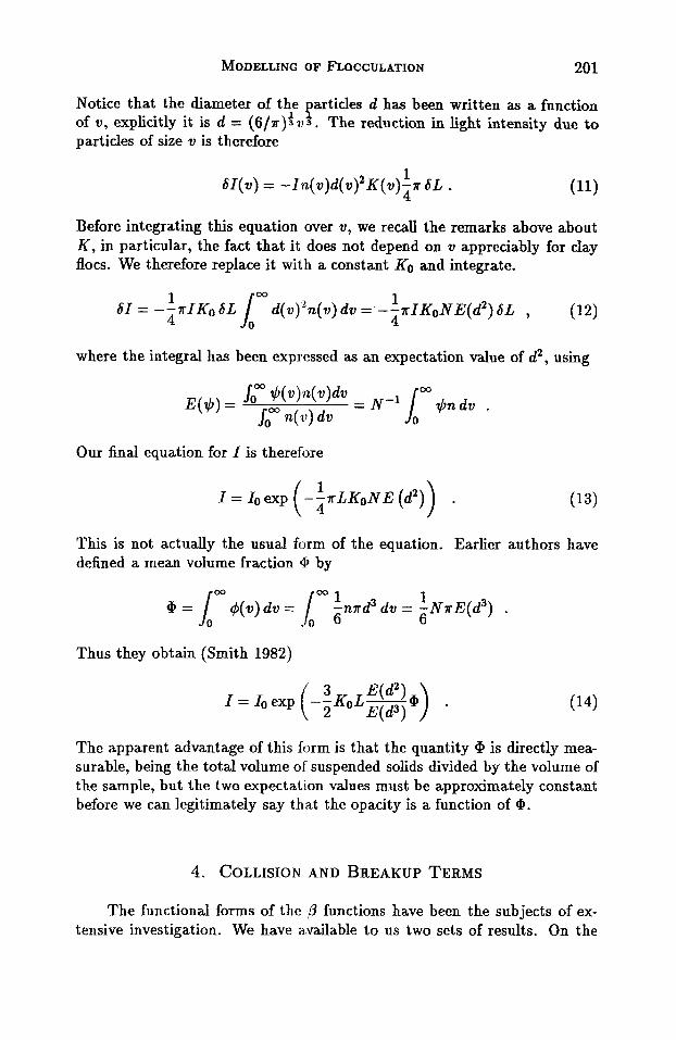
Notice that the diameter of the articles d has been written as a function of v, explicitly it is d = (6/7r)Sv3. The reduction in light intensity due to particles of size v is therefore

Y

Before integrating this equation over v, we recall the remarks above about K, in particular, the fact that it does not depend on v appreciably for clay flocs. We therefore replace it with a constant KO and integrate.

1 4

1 6 1 = ---TI& SL

4 d(v)2n(v) dv = --7rIK0lVE(d2) 6L , (12)

where the integral has been expressed as an expectation value of d 2 , using

Our final equation for I is therefore

This is not actually the usual form of the equation. Earlier authors have defined a mean volume fraction CP by

@ = lm q5(v)dv = dv = -N7rE(d3) 1 . 6

Thus they obtain (Smith 1982)

The apparent advantage of this form is that the quantity @ is directly mea- surable, being the total volume of suspended solids divided by the volume of the sample, but the two expectation values must be approximately constant before we can legitimately say that the opacity is a function of @.

4. COLLISION AND BREAKUP TERMS

The functional forms of the ,D functions have been the subjects of extensive investigation. We have available to us two sets of results. On the

202 D. J. JEFFREY

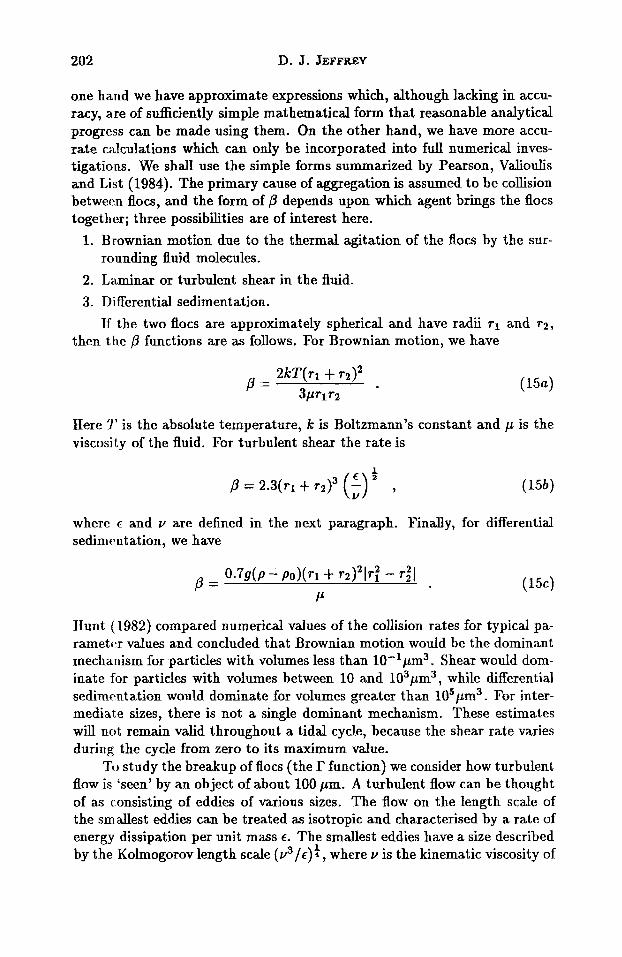
one hand we have approximate expressions which, although lacking in accuracy, are of sufficiently simple mathematical form that reasonable analytical progress can be made using them. On the other hand, we have more accurate calculations which can only be incorporated into full numerical investigations. We shall use the simple forms summarized by Pearson, Valioulis and List (1984). The primary cause of aggregation is assumed to be collision betwem flocs, and the form of p depends upon which agent brings the flocs together; three possibilities are of interest here.

1. Brownian motion due to the thermal agitation of the flocs by the sur- rounding fluid molecules.

2. Laminar or turbulent shear in the fluid. 3. Differential sedimentation.

If the two flocs are approximately spherical and have radii TI and ~ 2 ,

then the P functions are as follows. For Brownian motion, we have

Here ’1’ is the absolute temperature, k is Boltzmann’s constant and p is the viscosity of the fluid. For turbulent shear the rate is

where 6 and v are defined in the next paragraph. Finally, for differential sedimrntation, we have

Hunt (1982) compared numerical values of the collision rates for typical pa- rametc.r values and concluded that Brownian motion would be the dominant mechanism for particles with volumes less than 10-lpm3. Shear would dominate for particles with volumes between 10 and 103pm3, while differential sedimentation would dominate for volumes greater than 105pm3 - For inter- mediate sizes, there is not a single dominant mechanism. These estimates will not remain valid throughout a tidal cycle, because the shear rate varies during the cycle from zero to its maximum value.

To study the breakup of flocs (the I’ function) we consider how turbulent flow is ‘seen’ by an object of about 100 pm. A turbulent flow can be thought of as consisting of eddies of various sizes. The flow on the length scale of the smallest eddies can be treated as isotropic and characterised by a rate of energy dissipation per unit mass E . The smallest eddies have a size described by the Kolmogorov length scale (v3 /c) t , where Y is the kinematic viscosity of


the fluid, and the flow on scales smaller than this is laminar. In geophysical flows the Kolmogorov length is typically about 1 mm in size, and therefore objects as small as flocs can be treated its being in a laminar flow. This idea has been used in several contexts (Batchelor 1980; Maxey and Riley 1983). The problem to be solved is then reduced to finding the flow around a particle immersed in unbounded fluid with a known flow field imposed far from the particle. The randomness of the turbulence still makes itself felt, but in the lesser role of dictating the varying laminar flow that is imposed. Any fluid flowfield can be divided into an extension (or pure rate-of-strain) E and a rotation R. The rotation has little effect on the particle, since the particle simply spins at the same rotation rate as the fluid. The extension, on the other hand, will create a tension across the middle of the particle, tending to break it in half. The breakup is resisted by the attractive forces which caused the platelets to cohere in the first place, namely, the electrical forces between them. A standard calculation of the flow around a sphere in an extensional flow gives the tension between the halves as 37(3/4)37rspvf E.

We now need an expression for the force of cohesion within a floc. A model has been proposed to explain the strength of flocs by Krone (1978). Flocs are essentially brittle and become weaker as they grow larger. This is because the electrical attractive forces are short range and the stacking of the platelets in the floc becomes progressively less ideal. If the packing were the same for all sizes, we should expect the attractive force between the two (roughly) hemispherical halves of a floc to be proportional to the area of one face, i.e., proportional to 213. In fact a better fit to the experimental data is obtained with a strength proportional to vt. As we have seen, the rupturing fluid tension, however, is proportional to the surface area because it is unaffected by the internal structure, i-e. proportional to v f . In order for a floc to be ruptured by the flow, it must be in a part of the flow field in which the rate-of-strain produces a tension greater than the cohesive forces. This requires

2 1

2

where Q is an experimental coeflicient of cohesion with dimensions (for the present power law) of M T - 2 . The critical rate-of-strain is therefore

To obtain I' we must now integrate over all rates-of-strain greater than the critical one. Frenkiel and Klebanoff (1971) studied the distribution of velocity gradients in turbulent flow and their results can be approximated by saying that the probability density function P ( E ) for the rate-of-strain being

204 D. J. JEFFREY

equal to E is

Therefore the probability that the rate-of-strain will be larger in magnitude than .E, is

This criterion is an instantaneous one, in that, given a flow field at some instant of time, we obtain from (18) the number of flocs that break up. After the breakup, however, two things happen. The flowfield changes, and the flocs continue to aggregate. Therefore a breakup rate is obtained by taking into account the time scale of the flowfield. We have the number of flocs in the size range (0, v + dv) that break up as

dMb = n(v)P(E > E,) dv .

This number will not change until the flow field has evolved sufficient1 to be independent of the previous state. The time scale for this is ( v / c ) 2 / A , with A being a constant. Therefore, the rate of floc breakup becomes

r

1 r ( u ) = A ( z ) erfc ( 0 . 0 6 1 Q v - ~ p - ’ ( u ~ ) - f ) .

This formula uses the fact that u = p/p. We notice that as u becomes larger, the rate of breakup increases, as we expect.

5. QUASI-STATIONARY DISTRIBUTIONS

Friedlander (1960) introduced a set of approximate distribution functions, called quasi-stationary distributions, which were extended to clay suspensions by Hunt (1982). Friedlander, calling on ideas established in the theory of turbulence, observed that particle collisions created a flux of particles from smaller to larger sizes. For a distribution that has reached an equilibrium, this flux would be steady and constant for aU particle volumes. If in addition, only one collision mechanism were acting to cause aggregation, heidlander showed that dimensional analysis predicted a power law for n(v). Jeffrey (1981) turned the dimensional analysis into a rational set


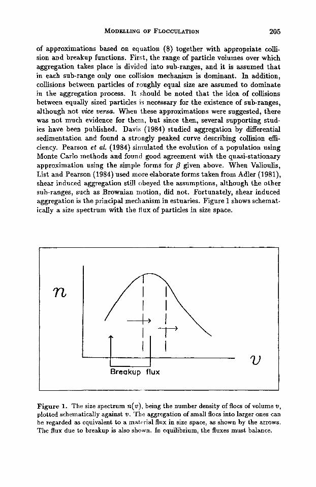
of approximations based on equation (8) together with appropriate collision and breakup functions. First, the range of particle volumes over which aggregation takes place is divided into sub-ranges, and it is assumed that in each sub-range only one collision mechanism is dominant. In addition, collisions between particles of roughly equal size are assumed to dominate in the aggregation process. It should be noted that the idea of collisions between equally sized particles i s necessary for the existence of sub-ranges, although not Vice versa. When these approximations were suggested, there was not much evidence for them, but since then, several supporting studies have been published. Davis (1984) studied aggregation by differential sedimentation and found a strongly peaked curve describing collision effi- ciency. Pearson et al. (1984) simulated the evolution of a population using Monte Carlo methods and found good agreement with the quasi-stationary approximation using the simple forms for /3 given above. When Valioulis, List and Pearson (1984) used more elaborate forms taken from Adler (1981), shear induced aggregation still obeyed the assumptions, although the other sub-ranges, such as Brownian motion, did not. Fortunately, shear induced aggregation is the principal mechanism in estuaries. Figure 1 shows schematically a size spectrum with the fiux of particles in size space.

n

Breakup flux

Figure 1. The size spectrum n(v) , being the number density of flocs of volume v, plotted schematically against O. The aggregation of small flocs into larger ones can be regarded as equivalent to a matcrial flux in size space, as shown by the arrows, The flux due to breakup is also shown. In equilibrium, the fluxes must balance.

206 D. J. JEFFREY

In order to use the same approach to solve the present equations, we must extend it to include the breakup term. Thus we must balance not just the first two integrals in (8) as Jeffrey (1981) did, but all three. Previously, it was argued that each integral containing p in (8) represented the flux of particle volume, and these were equal. Now we argue that the integrals still represent the flux of particles, but they are no longer equal, there being a difference between the flux of particles into any volume range from smaller particles aggregating, and the flux out of the range due to the creation of larger particles. The difference between these two fluxes is the breakup of the flocs. Using the expression for the flux given in Jeffrey (1981), we equate the rate of change of the flux with size range and the flux out of the size range due to breakup:

d -(pv3n2) = rvn . dv (20)

To solve this equation, we expand the derivative as

dn d dv dv

~ ~ ~ 2 ~ - + -((pv3)n2 = rvn.

We can now cancel a factor of n and use an integrating factor to obtain

Therefore

where v- indicates the minimum size for which the sub-range being used is defined and C is a constant of integration.

6. CALIBRATION OF TURBIDITY METERS

We now apply the above results to the calibration of turbidity meters. We bqgin by defining

1 v,j = 0.061&p-1(~~)- i . (22)

The volume represented by vo can be thought of as the smallest floc volume for which breakup is important. We now substitute the form of p corresponding to the shear sub-range into (21). In addition, in view of the interpretation, we equate vo and v - . Then

n = 0 . 1 1 A ~ - ~ /" erfc ($) v-' dv + O.&C ( 5 ) -' vW2 . "0 v3


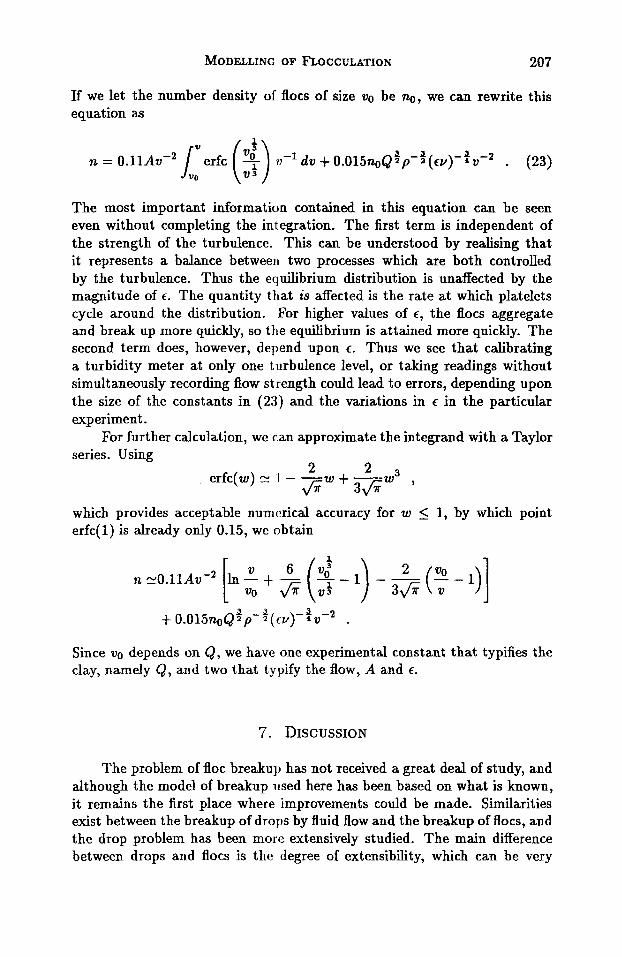
If we let the number density of flocs of size vo be no, we can rewrite this equation as

The most important information contained in this equation can be seen even without completing the integration. The first term is independent of the strength of the turbulence. This can be understood by realising that it represents a balance between two processes which are both controlled by the turbulence. Thus the equilibrium distribution is unaffected by the magnitude of 6. The quantity that is affected is the rate at which platelets cycle around the distribution. For higher values of e , the flocs aggregate and break up more quickly, so the equilibrium is attained more quickly. The second term does, however, depend upon E. Thus we see that calibrating a turbidity meter at only one turbulence level, or taking readings without simultaneously recording flow strength could lead to errors, depending upon the size of the constants in (23) and the variations in E in the particular experiment.

For further calculation, we can approximate the integrand with a Taylor series. Using

n n L L

erfc(w) N 1 - -w + - J. 3 f i W 3 , which provides acceptable numcrical accuracy for 'u) 5 1, by which point erfc(1) is already only 0.15, we obtain

Since vo depends on Q, we have one experimental constant that typifies the clay, namely Q, and two that typify the flow, A and E.

7. DISCUSSION

The problem of floc breakup has not received a great deal of study, and although the model of breakup used here has been based on what is known, it remains the first place where improvements could be made. Similarities exist between the breakup of drops by fluid flow and the breakup of flocs, and the drop problem has been more extensively studied. The main difference between drops and flocs is the degree of extensibility, which can be very

208 D. J. JEFFREY

large for drops, depending upon the ratio of internal to external viscosities and surface tension, but is not large for flocs. On the other hand, the effect of rotation as an inhibitor of breakup has been neglected here, but has been studied in detail for drops. In the present model, it was not possible to include the effects of rotation, because the time taken for the floc to deform and break was not taken into account: only an instantaneous breakup was considered. For drops, it is known that if there is rotation as well as extension, the part of the drop that has been extended can be rotated into a direction in which the flowfield is no longer extensional. The drop therefore has time to recover and resist breakup longer. Even for this effect, there is a limitation in the results in that the studies have been mostly for laminar flow and the stochastic nature of a turbulent flow field has not been addressed in the same detail.

The forms used for breakup and flocculation and the quai-stationary approximation should be taken together, in that they are all simple approximations that it would not be sensible to improve separately. The collision functions (15) do not include hydrodynamic forces between the flocs, and the calculation of these forces has been the subject of extensive investigations (Jeffrey and Onishi 1984). Similarly the number-density equation can be tackled numerically, or by direct simulation. Of course, for the purposes of reducing turbidity readings to densities, this degree of refinement seems unnectlssary and would certainly negate some of the speed of measurement which makes the instrument attractive.

We have been concerned here with modelling the dynamics of clay flocs. Part of the difficulty in constructing such models, both for the micromechan- ics of floc growth and breakup and for the global transport equations, is the lack of experimental data. This lack of data can be overcome only when measuring instruments have been developed which have a sufficient degree of power and reliability. And yet we have seen that that development requires some input from the models we are trying to construct. This circularity is well recognized by philosophers of science (Popper 1968). The development of physical models must therefore be recognized as an important part of environmental studies, and that, without it, many important areas of study will not be able to create the needed instruments of measurement or develop the necessary tools of understanding.

REFERENCES

Adler, P.M. (1981), “Heterocoagulation in shear flow”. Journal of Colloid Interface Science

Allen, 2’. (1975). Particle Size Measurement (2nd Ed.). Chapman and Hall. Basano, L., P. Ottonfello, and L. Papa (1976), “All-solid-state marine turbidimeter”. Deep-

Batchelor, G.K. (1980), “Mass transfer from small particles suspended in turbulent fluid”.

83, 106-115.

Sea Research 23, 187-190.

Journal of Fluid Mechanics 98, 609-623.


Davis, R.H. (1984), “The rate of coagulation of a dilute polydisperse system of sedimenting

Friedlander, S.K. (1960), ”Similarity considerations for the particlesize spectrum of a

Friedlander, S.K. (1977). Smoke, D u d and Haze. Wiley. Frenkiel, F.N. and P.S. Klebanoff (1971), “Statistical properties of velocity derivatives in

a turbulent field”. Journal of Fluid Mechanics 48, 183-208. Hom-ma, M. and K. Horikawa (1963), “A laboratory study on suspended sediment due

to wave action”. Proceedings of the 10th Congress, International Association for Hy- draulic Research 1, 213-220.

Hunt, J.R. (1982), “Self-similar particlesize distributions during coagulation: theory and experimental verification”. Journal of Fluid Mechanics 122, 169-185.

Jeffrey, D. J. (1981), “Quasi-stationary approximations for the size distribution of aerosols”. Journal of Atmospheric Science 38, 2440-2443.

Jeffrey, D.J. and Y. Onishi (1984), “Calculation of the resistance and mobility functions for two unequal rigid spheres in low-Reynolds-number flow”. Journal of Fluid Mechanics

Jones, D. and M.S. Wills (1956), “The attenuation of light in sea and estuarine waters in relation to the concentration of suspended solid matter”. Journal of the Marine Biological Association of the United Kingdom 35, 431-444.

Kirby, R. and W.R. Parker (1975), ”Sediment dynamics in the Severn Estuary: a back- ground for the study of the effects of a barrage”. In An Environmental Appraisal of the Seuern Barruge, (ed. T.L. Shaw). University of Bristol Press.

Kranck, K. (1981), “Particulate matter grain-size characteristics and flocculation in a partially mixed estuary”. Sedimentology 28, 107-114.

Krone, R.B. (1978), “Aggregation of suspended particles in estuaries”. In Estuarine Trans- port Processes (ed. B. Kjerfve). University of South Carolina Press.

Maxey, M.R. and J.J. Riley (1983), “Equation of motion for a small rigid sphere in a nonuniform flow”. Physics of Flurds 26, 883-889.

Pearson, H.J., I.A. Valioulis and E.J. List (1984), “Monte Carlo simulation of coagulation in discrete particle-size distributions. Part 1. Brownian motion and fluid shearing”. Journal of Fluid Mechanics 143 , 367-385.

spheres”. Journal of Fluid Mechanics 145, 179-199.

coagulating sedimenting aerosol”. Journal of Meteorology 17 ,479483.

139, 261-290.

Popper, K.R. (1968). The Logic of Scientific Discovery. Harper and Row. Rose, H.E. (19501, “ The design and use of phot+extinction sedimentometers”. Engineering

Smith, T.J. (1982). Report No 137. ‘The response of electro-optical turbidity meters to cohesive sediments. Institute of Oceanographic Sciences, Taunton, UK.

Valioulis, I.A., E.J. List and H.J. Pearson (1984), “Monte Carlo simulation of coagulation in discrete particlesize distributions. Part 2. Interparticle forces and the quasi-stationary hypothesis”. Journal of Fluid Mechanics 143, 387411.

169, 350-351.

Documents

Sediment transport: Physical modelling of flocculation