Seismic interpretation below tuning with multiattribute ... · Seismic interpretation below tuning with multiattribute analysis Abstract he tuning-bed thickness or vertical resolution

330 THE LEADING EDGE April 2017

Seismic interpretation below tuning with multiattribute analysis

AbstractThe tuning-bed thickness or vertical resolution of seismic data

traditionally is based on the frequency content of the data and the associated wavelet. Seismic interpretation of thin beds routinely involves estimation of tuning thickness and the subsequent scaling of amplitude or inversion information below tuning. These tra-ditional below-tuning-thickness estimation approaches have limitations and require assumptions that limit accuracy. The below-tuning effects are a result of the interference of wavelets, which are a function of the geology as it changes vertically and laterally. However, numerous instantaneous attributes exhibit effects at and below tuning, but these are seldom incorporated in thin-bed analyses. A seismic multiattribute approach employs self-orga-nizing maps to identify natural clusters from combinations of attributes that exhibit below-tuning effects. These results may exhibit changes as thin as a single sample interval in thickness. Self-organizing maps employed in this fashion analyze associated seismic attributes on a sample-by-sample basis and identify the natural patterns or clusters produced by thin beds. This thin-bed analysis utilizing self-organizing maps has been corroborated with extensive well control to verify consistent results. Therefore, thin beds identified with this methodology enable more accurate mapping of facies below tuning and are not restricted by traditional frequency limitations.

IntroductionFundamental to the evaluation of a prospect or development

of a field is the seismic interpretation of the vertical resolution or tuning thickness of the associated seismic data. This interpretation has significant implications in understanding the geologic facies and stratigraphy, the determination of reservoir thickness above and/or below tuning, delineation of direct hydrocarbon indicators (DHIs), and project economic and risk assessment. The foundations of our understanding of seismic vertical resolution come from the influential research by Ricker (1953), Widess (1973), and Kallweit and Wood (1982). The conventionally accepted definition of the tuning thickness is a bed that is ¼ wavelength in thickness, for which reflections from its upper and lower surfaces interfere con-structively where the interface contrasts are of opposite polarity, resulting in an exceptionally strong reflection (Sheriff, 2002). Below tuning, the time separation of the reflections from the top and bottom of a reservoir essentially do not change, and the thickness must be determined by other methods. Some of the earliest work in determining bed thickness below tuning was by Meckel and Nath (1977), Neidell and Poggiagliolmi (1977), and Schramm et al. (1977), who related the normalized or sum of the absolute value amplitudes of the top and bottom reflections of a thin bed to have a linear relationship to net thickness of sands. Brown et al. (1984, 1986) employed seismic crossplots of gross isochron thickness versus composite amplitude to determine an amplitude scalar to calculate

Rocky Roden1, Thomas A. Smith1, Patricia Santogrossi1, Deborah Sacrey2, and Gary Jones1

net pay. With sufficient well calibration, Connolly (2007) presented a map-based amplitude-scaling technique based on band-limited impedance through colored inversion for thin-bed determination. As Simm (2009) indicates, various techniques to determine thin beds have limitations and require assumptions that may not be met all of the time. Therefore, what is required is an approach that exploits other properties of thin beds even though our fundamental understanding of seismic amplitudes and time separation of reflec-tions from the top and bottom of a reservoir implies this cannot be done consistently and accurately with conventional amplitude data. A seismic multiattribute approach takes advantage of analyzing several attributes at each instant of time and identifies patterns from these data to produce results below tuning that relate to bed thickness and stratigraphy.

BackgroundA seismic attribute is any measureable property of seismic

data, such as amplitude, dip, phase, frequency, and polarity that can be measured at one instant in time/depth, over a time/depth window, on a single trace, on a set of traces, or on a surface in-terpreted from the seismic data (Schlumberger Oilfield Glossary). Instantaneous seismic attributes are quantities computed sample by sample at a time/depth instance and indicate continuous change in properties along the time and space axis. The original instan-taneous attributes are features of a complex seismic trace and are based on the analytical signal of the original trace and its Hilbert transform; these include instantaneous amplitude (envelope), instantaneous phase, and instantaneous frequency. Taner and Sheriff (1977) state that the conventional seismic trace may be thought of as a measure of kinetic energy, and as a wavefront passes through the earth, the particle motion is resisted by an elastic restoring force so that energy becomes stored as potential energy. The Hilbert transform may be thought of as a measure of elastic potential energy. Therefore the measured seismic amplitude trace and the complex trace attributes, as well as the dozens of attributes derived from them over the last few decades, represent instantaneous attributes that define the kinetic and potential energy of the seismic trace through space and time/depth.

Robertson and Nogami (1984) and Tirado (2004) identified a frequency increase or frequency tuning effect below conventional seismic tuning. Hardage et al. (1998), Radovich and Oliveros (1998), Taner (2003), and Zeng (2010) confirmed the relationship of frequency spikes and bed thickness on instantaneous frequency data but, in general, recommend the integration of lithofacies and depositional facies analysis because of the nonuniqueness of the frequency attribute. From instantaneous phase and frequency data, Davogustto et al. (2013) identified phase discontinuities that produce phase residues above and below tuning depending on the frequency content of the data. Zeng (2015) showed with wedge models that a 90° phase-rotated wavelet, similar to the

1Geophysical Insights.2Auburn Energy.

http://dx.doi.org/10.1190/tle36040330.1.

April 2017 THE LEADING EDGE 331

Hilbert transform, produces better definition of beds below tuning than zero-phase wavelets. This research has identified various phenomena at or below tuning, but consistent interpretation of thin beds is still a challenge and requires another approach.

Multiattribute analysisIn an effort to understand which instantaneous attributes

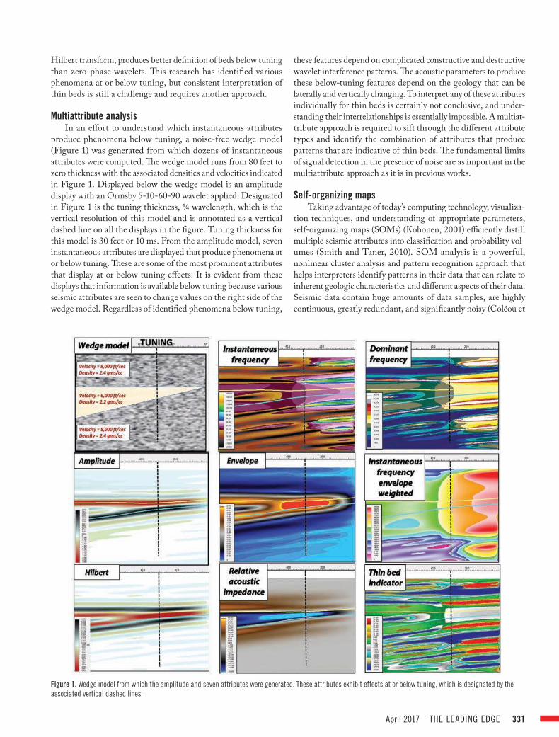
produce phenomena below tuning, a noise-free wedge model (Figure 1) was generated from which dozens of instantaneous attributes were computed. The wedge model runs from 80 feet to zero thickness with the associated densities and velocities indicated in Figure 1. Displayed below the wedge model is an amplitude display with an Ormsby 5-10-60-90 wavelet applied. Designated in Figure 1 is the tuning thickness, ¼ wavelength, which is the vertical resolution of this model and is annotated as a vertical dashed line on all the displays in the figure. Tuning thickness for this model is 30 feet or 10 ms. From the amplitude model, seven instantaneous attributes are displayed that produce phenomena at or below tuning. These are some of the most prominent attributes that display at or below tuning effects. It is evident from these displays that information is available below tuning because various seismic attributes are seen to change values on the right side of the wedge model. Regardless of identified phenomena below tuning,

these features depend on complicated constructive and destructive wavelet interference patterns. The acoustic parameters to produce these below-tuning features depend on the geology that can be laterally and vertically changing. To interpret any of these attributes individually for thin beds is certainly not conclusive, and under-standing their interrelationships is essentially impossible. A multiat-tribute approach is required to sift through the different attribute types and identify the combination of attributes that produce patterns that are indicative of thin beds. The fundamental limits of signal detection in the presence of noise are as important in the multiattribute approach as it is in previous works.

Self-organizing mapsTaking advantage of today’s computing technology, visualiza-

tion techniques, and understanding of appropriate parameters, self-organizing maps (SOMs) (Kohonen, 2001) efficiently distill multiple seismic attributes into classification and probability vol-umes (Smith and Taner, 2010). SOM analysis is a powerful, nonlinear cluster analysis and pattern recognition approach that helps interpreters identify patterns in their data that can relate to inherent geologic characteristics and different aspects of their data. Seismic data contain huge amounts of data samples, are highly continuous, greatly redundant, and significantly noisy (Coléou et

Figure 1. Wedge model from which the amplitude and seven attributes were generated. These attributes exhibit effects at or below tuning, which is designated by the

associated vertical dashed lines.


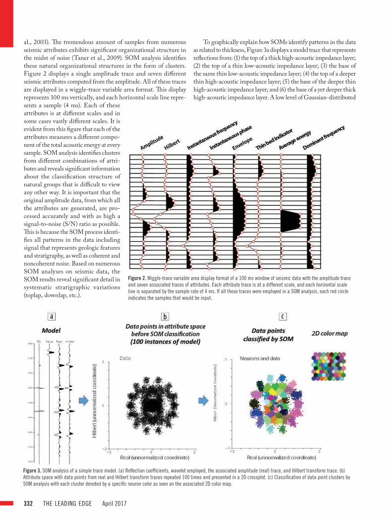
al., 2003). The tremendous amount of samples from numerous seismic attributes exhibits significant organizational structure in the midst of noise (Taner et al., 2009). SOM analysis identifies these natural organizational structures in the form of clusters. Figure 2 displays a single amplitude trace and seven different seismic attributes computed from the amplitude. All of these traces are displayed in a wiggle-trace variable area format. This display represents 100 ms vertically, and each horizontal scale line repre-sents a sample (4 ms). Each of these attributes is at different scales and in some cases vastly different scales. It is evident from this figure that each of the attributes measures a different compo-nent of the total acoustic energy at every sample. SOM analysis identifies clusters from different combinations of attri-butes and reveals significant information about the classification structure of natural groups that is difficult to view any other way. It is important that the original amplitude data, from which all the attributes are generated, are pro-cessed accurately and with as high a signal-to-noise (S/N) ratio as possible. This is because the SOM process identi-fies all patterns in the data including signal that represents geologic features and stratigraphy, as well as coherent and noncoherent noise. Based on numerous SOM analyses on seismic data, the SOM results reveal significant detail in systematic stratigraphic variations (toplap, downlap, etc.).

To graphically explain how SOMs identify patterns in the data as related to thickness, Figure 3a displays a model trace that represents reflections from: (1) the top of a thick high-acoustic impedance layer; (2) the top of a thin low-acoustic impedance layer; (3) the base of the same thin low-acoustic impedance layer; (4) the top of a deeper thin high-acoustic impedance layer; (5) the base of the deeper thin high-acoustic impedance layer; and (6) the base of a yet deeper thick high-acoustic impedance layer. A low level of Gaussian-distributed

Figure 2. Wiggle-trace variable area display format of a 100 ms window of seismic data with the amplitude trace

and seven associated traces of attributes. Each attribute trace is at a different scale, and each horizontal scale

line is separated by the sample rate of 4 ms. If all these traces were employed in a SOM analysis, each red circle

indicates the samples that would be input.

Figure 3. SOM analysis of a simple trace model. (a) Reflection coefficients, wavelet employed, the associated amplitude (real) trace, and Hilbert transform trace. (b)

Attribute space with data points from real and Hilbert transform traces repeated 100 times and presented in a 2D crossplot. (c) Classification of data point clusters by

SOM analysis with each cluster denoted by a specific neuron color as seen on the associated 2D color map.


reflection coefficient noise was added. A wavelet centered at 30 Hz and a bandwidth of 40 Hz was applied to the reflection coefficients in Figure 3a. The sample interval is 2 ms, which is the thickness of the two thin beds in the model. Conventional tuning thickness is 12 ms. From the amplitude trace (labeled real), the Hilbert transform was generated and resulted in 411 samples of paired values. The real and Hilbert transform analytic traces were realized 100 times to produce a significant number of data points. The set of 41,100 data point pairs were input into a SOM analysis.

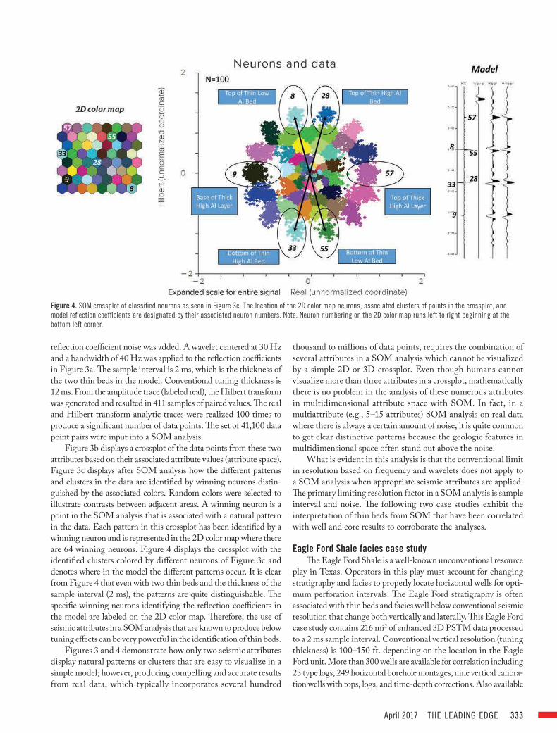
Figure 3b displays a crossplot of the data points from these two attributes based on their associated attribute values (attribute space). Figure 3c displays after SOM analysis how the different patterns and clusters in the data are identified by winning neurons distin-guished by the associated colors. Random colors were selected to illustrate contrasts between adjacent areas. A winning neuron is a point in the SOM analysis that is associated with a natural pattern in the data. Each pattern in this crossplot has been identified by a winning neuron and is represented in the 2D color map where there are 64 winning neurons. Figure 4 displays the crossplot with the identified clusters colored by different neurons of Figure 3c and denotes where in the model the different patterns occur. It is clear from Figure 4 that even with two thin beds and the thickness of the sample interval (2 ms), the patterns are quite distinguishable. The specific winning neurons identifying the reflection coefficients in the model are labeled on the 2D color map. Therefore, the use of seismic attributes in a SOM analysis that are known to produce below tuning effects can be very powerful in the identification of thin beds.

Figures 3 and 4 demonstrate how only two seismic attributes display natural patterns or clusters that are easy to visualize in a simple model; however, producing compelling and accurate results from real data, which typically incorporates several hundred

thousand to millions of data points, requires the combination of several attributes in a SOM analysis which cannot be visualized by a simple 2D or 3D crossplot. Even though humans cannot visualize more than three attributes in a crossplot, mathematically there is no problem in the analysis of these numerous attributes in multidimensional attribute space with SOM. In fact, in a multiattribute (e.g., 5–15 attributes) SOM analysis on real data where there is always a certain amount of noise, it is quite common to get clear distinctive patterns because the geologic features in multidimensional space often stand out above the noise.

What is evident in this analysis is that the conventional limit in resolution based on frequency and wavelets does not apply to a SOM analysis when appropriate seismic attributes are applied. The primary limiting resolution factor in a SOM analysis is sample interval and noise. The following two case studies exhibit the interpretation of thin beds from SOM that have been correlated with well and core results to corroborate the analyses.

Eagle Ford Shale facies case studyThe Eagle Ford Shale is a well-known unconventional resource

play in Texas. Operators in this play must account for changing stratigraphy and facies to properly locate horizontal wells for opti-mum perforation intervals. The Eagle Ford stratigraphy is often associated with thin beds and facies well below conventional seismic resolution that change both vertically and laterally. This Eagle Ford case study contains 216 mi2 of enhanced 3D PSTM data processed to a 2 ms sample interval. Conventional vertical resolution (tuning thickness) is 100–150 ft. depending on the location in the Eagle Ford unit. More than 300 wells are available for correlation including 23 type logs, 249 horizontal borehole montages, nine vertical calibra-tion wells with tops, logs, and time-depth corrections. Also available

Figure 4. SOM crossplot of classified neurons as seen in Figure 3c. The location of the 2D color map neurons, associated clusters of points in the crossplot, and

model reflection coefficients are designated by their associated neuron numbers. Note: Neuron numbering on the 2D color map runs left to right beginning at the

bottom left corner.


are five cores for which X-ray diffraction and saturation information was available. This well information was incorporated in the cor-roboration of the SOM results.

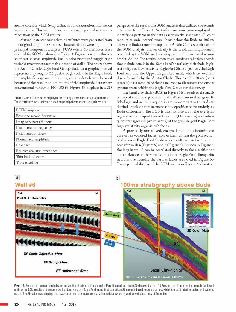
Sixteen instantaneous seismic attributes were generated from the original amplitude volume. These attributes were input into a principal component analysis (PCA) where 10 attributes were selected for SOM analysis (see Table 1). Figure 5a is a northwest-southeast seismic amplitude line in color raster and wiggle-trace variable area formats across the location of well 6. The figure shows the Austin Chalk-Eagle Ford Group-Buda stratigraphic interval represented by roughly 2.5 peak/trough cycles. In the Eagle Ford, the amplitude appears continuous, yet any details are obscured because of the resolution limitations of the amplitude data where conventional tuning is 100–150 ft. Figure 5b displays in a 3D

perspective the results of a SOM analysis that utilized the seismic attributes from Table 1. Sixty-four neurons were employed to identify 64 patterns in the data as seen on the associated 2D color map. A seismic interval from 10 ms below the Buda to 100 ms above the Buda or near the top of the Austin Chalk was chosen for the SOM analysis. Shown clearly is the resolution improvement provided by the SOM analysis compared to the associated seismic amplitude line. The results shown reveal nonlayer cake facies bands that include details in the Eagle Ford’s basal clay-rich shale, high-resistivity and low-resistivity Eagle Ford Shale objectives, the Eagle Ford ash, and the Upper Eagle Ford marl, which are overlain disconformably by the Austin Chalk. This roughly 28 ms (or 14 samples) uses some 26 of the 64 neurons to illuminate the various systems tracts within the Eagle Ford Group for this survey.

The basal clay shale (BCS) in Figure 5b is resolved distinctly on top of the Buda generally by the #1 neuron in dark gray. Its lithologic and neural uniqueness are concomitant with its distal detrital or pelagic emplacement after deposition of the underlying Buda carbonates. The BCS is distinct also from the overlying regressive downlap of two red neurons (black arrow) and subse-quent transgressive (white arrow) of the grayish-gold Eagle Ford high-resistivity organic rich facies.

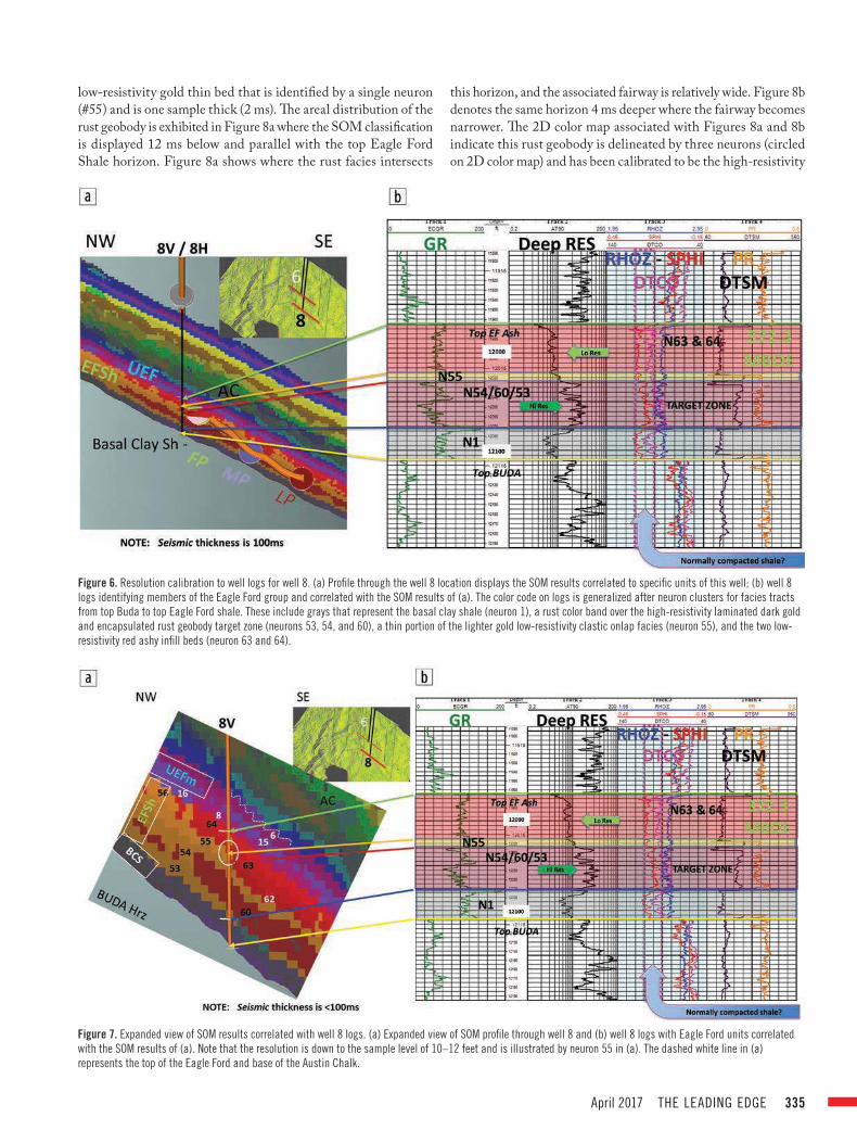
A previously unresolved, encapsulated, and discontinuous core of rust-colored facies, now evident within the gold section of the lower Eagle Ford Shale is also well resolved in the pilot holes for wells 6 (Figure 5) and 8 (Figure 6). As seen in Figure 6, the logs in well 8 can be correlated directly to the classification and thicknesses of the various units in the Eagle Ford. The specific neurons that identify the various facies are noted in Figure 6b. The expanded display of the SOM results in Figure 7a denotes a

Figure 5. Resolution comparison between conventional seismic display and a Paradise multiattribute SOM classification. (a) Seismic amplitude profile through the 6 well

and (b) the SOM results of the same profile identifying the Eagle Ford group that comprises 26 sample-based neuron clusters, which are calibrated to facies and systems

tracts. The 2D color map displays the associated neuron cluster colors. Seismic data owned by and provided courtesy of Seitel Inc.

PSTM amplitude

Envelope second derivative

Imaginary part (Hilbert)

Instantaneous frequency

Instantaneous phase

Normalized amplitude

Real part

Relative acoustic impedance

Thin-bed indicator

Trace envelope

Table 1. Seismic attributes employed for the Eagle Ford case study SOM analysis.

These attributes were selected based on principal component analysis results.


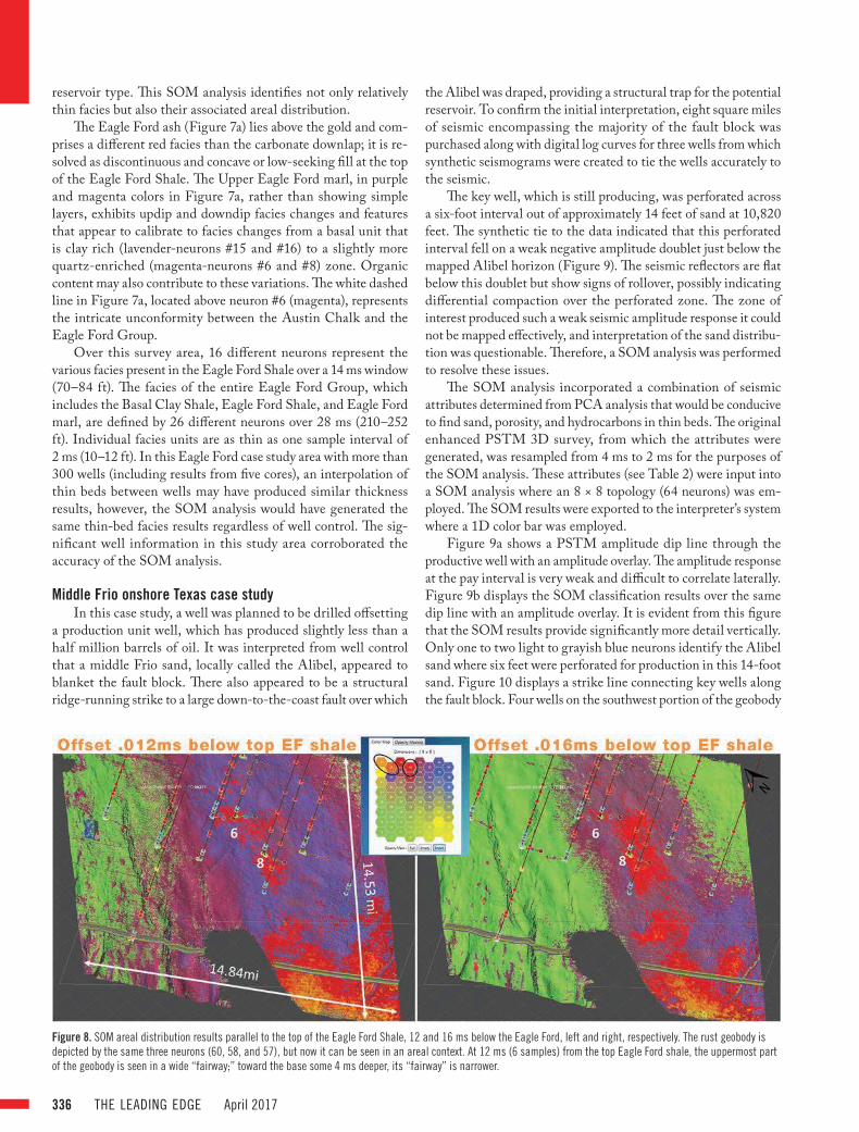
low-resistivity gold thin bed that is identified by a single neuron (#55) and is one sample thick (2 ms). The areal distribution of the rust geobody is exhibited in Figure 8a where the SOM classification is displayed 12 ms below and parallel with the top Eagle Ford Shale horizon. Figure 8a shows where the rust facies intersects

this horizon, and the associated fairway is relatively wide. Figure 8b denotes the same horizon 4 ms deeper where the fairway becomes narrower. The 2D color map associated with Figures 8a and 8b indicate this rust geobody is delineated by three neurons (circled on 2D color map) and has been calibrated to be the high-resistivity

Figure 6. Resolution calibration to well logs for well 8. (a) Profile through the well 8 location displays the SOM results correlated to specific units of this well; (b) well 8

logs identifying members of the Eagle Ford group and correlated with the SOM results of (a). The color code on logs is generalized after neuron clusters for facies tracts

from top Buda to top Eagle Ford shale. These include grays that represent the basal clay shale (neuron 1), a rust color band over the high-resistivity laminated dark gold

and encapsulated rust geobody target zone (neurons 53, 54, and 60), a thin portion of the lighter gold low-resistivity clastic onlap facies (neuron 55), and the two low-

resistivity red ashy infill beds (neuron 63 and 64).

Figure 7. Expanded view of SOM results correlated with well 8 logs. (a) Expanded view of SOM profile through well 8 and (b) well 8 logs with Eagle Ford units correlated

with the SOM results of (a). Note that the resolution is down to the sample level of 10–12 feet and is illustrated by neuron 55 in (a). The dashed white line in (a)

represents the top of the Eagle Ford and base of the Austin Chalk.


reservoir type. This SOM analysis identifies not only relatively thin facies but also their associated areal distribution.

The Eagle Ford ash (Figure 7a) lies above the gold and com-prises a different red facies than the carbonate downlap; it is re-solved as discontinuous and concave or low-seeking fill at the top of the Eagle Ford Shale. The Upper Eagle Ford marl, in purple and magenta colors in Figure 7a, rather than showing simple layers, exhibits updip and downdip facies changes and features that appear to calibrate to facies changes from a basal unit that is clay rich (lavender-neurons #15 and #16) to a slightly more quartz-enriched (magenta-neurons #6 and #8) zone. Organic content may also contribute to these variations. The white dashed line in Figure 7a, located above neuron #6 (magenta), represents the intricate unconformity between the Austin Chalk and the Eagle Ford Group.

Over this survey area, 16 different neurons represent the various facies present in the Eagle Ford Shale over a 14 ms window (70–84 ft). The facies of the entire Eagle Ford Group, which includes the Basal Clay Shale, Eagle Ford Shale, and Eagle Ford marl, are defined by 26 different neurons over 28 ms (210–252 ft). Individual facies units are as thin as one sample interval of 2 ms (10–12 ft). In this Eagle Ford case study area with more than 300 wells (including results from five cores), an interpolation of thin beds between wells may have produced similar thickness results, however, the SOM analysis would have generated the same thin-bed facies results regardless of well control. The sig-nificant well information in this study area corroborated the accuracy of the SOM analysis.

Middle Frio onshore Texas case studyIn this case study, a well was planned to be drilled offsetting

a production unit well, which has produced slightly less than a half million barrels of oil. It was interpreted from well control that a middle Frio sand, locally called the Alibel, appeared to blanket the fault block. There also appeared to be a structural ridge-running strike to a large down-to-the-coast fault over which

the Alibel was draped, providing a structural trap for the potential reservoir. To confirm the initial interpretation, eight square miles of seismic encompassing the majority of the fault block was purchased along with digital log curves for three wells from which synthetic seismograms were created to tie the wells accurately to the seismic.

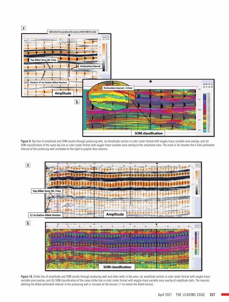
The key well, which is still producing, was perforated across a six-foot interval out of approximately 14 feet of sand at 10,820 feet. The synthetic tie to the data indicated that this perforated interval fell on a weak negative amplitude doublet just below the mapped Alibel horizon (Figure 9). The seismic reflectors are flat below this doublet but show signs of rollover, possibly indicating differential compaction over the perforated zone. The zone of interest produced such a weak seismic amplitude response it could not be mapped effectively, and interpretation of the sand distribu-tion was questionable. Therefore, a SOM analysis was performed to resolve these issues.

The SOM analysis incorporated a combination of seismic attributes determined from PCA analysis that would be conducive to find sand, porosity, and hydrocarbons in thin beds. The original enhanced PSTM 3D survey, from which the attributes were generated, was resampled from 4 ms to 2 ms for the purposes of the SOM analysis. These attributes (see Table 2) were input into a SOM analysis where an 8 × 8 topology (64 neurons) was em-ployed. The SOM results were exported to the interpreter’s system where a 1D color bar was employed.

Figure 9a shows a PSTM amplitude dip line through the productive well with an amplitude overlay. The amplitude response at the pay interval is very weak and difficult to correlate laterally. Figure 9b displays the SOM classification results over the same dip line with an amplitude overlay. It is evident from this figure that the SOM results provide significantly more detail vertically. Only one to two light to grayish blue neurons identify the Alibel sand where six feet were perforated for production in this 14-foot sand. Figure 10 displays a strike line connecting key wells along the fault block. Four wells on the southwest portion of the geobody

Figure 8. SOM areal distribution results parallel to the top of the Eagle Ford Shale, 12 and 16 ms below the Eagle Ford, left and right, respectively. The rust geobody is

depicted by the same three neurons (60, 58, and 57), but now it can be seen in an areal context. At 12 ms (6 samples) from the top Eagle Ford shale, the uppermost part

of the geobody is seen in a wide “fairway;” toward the base some 4 ms deeper, its “fairway” is narrower.


Figure 9. Dip line of amplitude and SOM results through producing well. (a) Amplitude section in color raster format with wiggle-trace variable area overlay; and (b)

SOM classification of the same dip line in color raster format with wiggle-trace variable area overlay of the amplitude data. The inset in (b) denotes the 6-foot perforated

interval of the producing well correlated to the light to grayish blue neurons.

Figure 10. Strike line of amplitude and SOM results through producing well and other wells in the area: (a) amplitude section in color raster format with wiggle-trace

variable area overlay; and (b) SOM classification of the same strike line in color raster format with wiggle-trace variable area overlay of amplitude data. The neurons

defining the Alibel perforated interval in the producing well is situated at the horizon 17 ms below the Alibel horizon.


did not produce significant amounts of hydrocarbons and were thought to have been “mechanical failures.” However, after a review of the sand distribution based upon time slices through the interval (see Figure 11), it was determined that they were isolated in localized areas or on the fringes of the bar system and not connected to the main body of sand. Figure 10a is the PSTM amplitude strike line that exhibits very little amplitude or character in the Alibel interval. This same line in Figure 10b shows the SOM classification, which exhibits the detail and variability of the stratigraphy for this area.

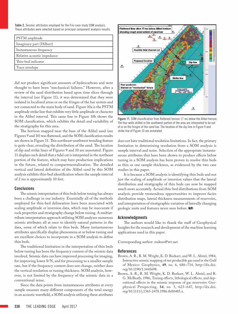
The horizon mapped near the base of the Alibel sand (see Figures 9 and 10) was flattened, and the SOM classification results are shown in Figure 11. This northeast-southwest trending feature is quite clear, revealing the distribution of the sand. The location of dip and strike lines of Figures 9 and 10 are annotated. Figure 11 displays such detail that a tidal cut is interpreted in the northeast portion of the feature, which may have production implications in the future, related to compartmentalization. The detailed vertical and lateral definition of the Alibel sand by this SOM analysis exhibits thin-bed identification where the sample interval of 2 ms is approximately 10 feet.

ConclusionsThe seismic interpretation of thin beds below tuning has always

been a challenge in our industry. Essentially all of the methods employed for thin-bed delineation have been associated with scaling amplitude or inversion data, which may be inaccurate if rock properties and stratigraphy change below tuning. A multiat-tribute interpretation approach utilizing SOM analyzes numerous seismic attributes all at once to identify natural patterns in the data, some of which relate to thin beds. Many instantaneous attributes specifically display phenomena at or below tuning and are excellent choices to incorporate in a SOM analysis to define thin beds.

The traditional limitation in the interpretation of thin beds below tuning has been the frequency content of the seismic data involved. Seismic data can have improved processing for imaging, for improving lower S/N, and for processing to a smaller sample rate, but if the frequency content does not change, neither does the vertical resolution or tuning thickness. SOM analysis, how-ever, is not limited by the frequency of the seismic data in a conventional sense.

Since the data points from instantaneous attributes at every sample measure many different components of the total energy in an acoustic wavefield, a SOM analysis utilizing these attributes

does not have traditional resolution limitations. In fact, the primary limitation in determining resolution from a SOM analysis is sample interval and noise. Selection of the appropriate instanta-neous attributes that have been shown to produce effects below tuning in a SOM analysis has been proven to resolve thin beds as thin as one sample thickness, as evidenced by the two case studies in this paper.

It is because a SOM analysis is identifying thin beds and not just the scaling of amplitude or inversion values that the lateral distribution and stratigraphy of thin beds can now be mapped much more accurately. Actual thin-bed distributions from SOM analysis provide tremendous opportunities to improve facies distribution maps, lateral thickness measurements of reservoirs, and interpretation of stratigraphic variation of laterally changing geologic units and features never seen before.

AcknowledgmentsThe authors would like to thank the staff of Geophysical

Insights for the research and development of the machine learning applications used in this paper.

Corresponding author: [email protected]

ReferencesBrown, A. R., R. M. Wright, K. D. Burkart, and W. L. Abriel, 1984,

Interactive seismic mapping of net producible gas sand in the Gulf of Mexico: Geophysics, 49, no. 6, 686–714, http://dx.doi.org/10.1190/1.1441698.

Brown, A. R., R. M. Wright, K. D. Burkart, W. L. Abriel, and R. G. McBeath, 1986, Tuning effects, lithological effects, and dep-ositional effects in the seismic response of gas reservoirs: Geo-physical Prospecting, 34, no. 5, 623–647, http://dx.doi.org/10.1111/j.1365-2478.1986.tb00485.x.

Figure 11. SOM classification from flattened horizon 17 ms below the Alibel horizon.

The four wells drilled in the southwest portion of the area are interpreted to be out

of or on the fringes of the sand bar. The location of the dip line in Figure 9 and

strike line of Figure 10 are annotated.

PSTM amplitude

Imaginary part (Hilbert)

Instantaneous frequency

Relative acoustic impedance

Thin-bed indicator

Trace envelope

Table 2. Seismic attributes employed for the Frio case study SOM analysis.

These attributes were selected based on principal component analysis results.


Coléou, T., M. Poupon, and K. Azbel, 2003, Unsupervised seismic facies classification: A review and comparison of techniques and implementation: The Leading Edge, 22, no. 10, 942–953, http://dx.doi.org/10.1190/1.1623635.

Connolly, P., 2007, A simple, robust algorithm for seismic net pay estimation: The Leading Edge, 26, no. 10, 1278–1282, http://dx.doi.org/10.1190/1.2794386.

Davogustto, O., M. C. de Matos, C. Cabarcas, T. Dao, and K. J. Marfurt, 2013, Resolving subtle stratigraphic features using spec-tral ridges and phase residues: Interpretation, 1, no. 1, SA93–SA108, http://dx.doi.org/10.1190/INT-2013-0015.1.

Hardage, B. A., V. M. Pendleton, J. L. Simmons Jr., B. A. Stubbs, and B. J. Uszynski, 1998, 3-D instantaneous frequency used as a coherency/continuity parameter to interpret reservoir compart-ment boundaries across an area of complex turbidite deposition: Geophysics, 63, no. 5, 1520–1531, http://dx.doi.org/10.1190/1.1444448.

Kallweit, R. S., and L. C. Wood, 1982, The limits of resolution of zero-phase wavelets: Geophysics, 47, no. 7, 1035–1046, http://dx.doi.org/10.1190/1.1441367.

Kohonen, T., 2001, Self-organizing maps: Third extended addition, v. 30: Springer Series in Information Services.

Meckel, L. D., and A. K. Nath, 1977, Geologic consideration for stratigraphic modelling and interpretation, in C. E. Payton, ed., Seismic stratigraphy — Applications to hydrocarbon exploration: AAPG Memoir 26, 417–438.

Neidell, N. S., and E. Poggiagliolmi, 1977, Stratigraphic modeling and interpretation —Geophysical principles and techniques, in C. E. Payton, ed., Seismic stratigraphy —Applications to hydro-carbon exploration: AAPG Memoir 26, 389–416.

Radovich, B. J., and B. Oliveros, 1998, 3-D sequence interpretation of seismic instantaneous attributes from the Gorgon Field: The Leading Edge, 17, no. 9, 1286–1293, http://dx.doi.org/10.1190/1.1438125.

Ricker, N., 1953, Wavelet contraction, wavelet expansion, and the control of seismic resolution: Geophysics, 18, no. 4, 769–792, http://dx.doi.org/10.1190/1.1437927.

Robertson, J. D., and H. H. Nogami, 1984, Complex seismic trace analysis of thin beds: Geophysics, 49, no. 4, 344–352, http://dx.doi.org/10.1190/1.1441670.

Schlumberger Oilfield Glossary, http://www.glossary.oilfield.slb.com, accessed 31 January 2017.

Schramm, M. W. Jr., E. V. Dedman, and J. P. Lindsey, 1977, Prac-tical stratigraphic modeling and interpretation, in C. E. Payton, ed., Seismic stratigraphy — Applications to hydrocarbon explo-ration: AAPG Memoir 26, 477–502.

Sheriff, R. E., 2002, Encyclopedic Dictionary of Applied Geophys-ics, 4th ed.: SEG.

Simm, R. W., 2009, Simple net pay estimation from seismic: A mod-elling study: First Break, 27, no. 1304, 45–53, http://dx.doi.org/10.3997/1365-2397.2009014.

Smith, T., and M. T. Taner, 2010, Natural clusters in multi-attri-bute seismics found with self-organizing maps: Extended Ab-stracts, Robinson-Treitel Spring Symposium, GSH/SEG.

Taner, M. T., S. Treitel, and T. Smith, 2009, Self-organizing maps of multi-attribute 3D seismic reflection surveys: SEG.

Taner, M. T., and R. E. Sheriff, 1977, Application of amplitude, fre-quency, and other attributes to stratigraphic and hydrocarbon de-termination, in C. E. Payton, ed., Seismic stratigraphy — Ap-plications to hydrocarbon exploration: AAPG Memoir 26, 301–327.

Taner, M. T., 2003, Attributes revisited, http://www.rocksolidim-ages.com/pdf/attrib_revisited.htm, accessed 13 August 2013.

Tirado, S., 2004, Sand thickness estimation using spectral decom-position, MS Thesis, University of Oklahoma.

Widess, M. B., 1973, How thin is a thin bed?: Geophysics, 38, no. 6, 1176–1180, http://dx.doi.org/10.1190/1.1440403.

Zeng, H., 2010, Geologic significance of anomalous instantaneous frequency: Geophysics, 75, no. 3, P23–P30, http://dx.doi.org/10.1190/1.3427638.

Zeng, H., 2015, Predicting geometry and stacking pattern of thin beds by interpreting geomorphology and waveforms using se-quential stratal-slices in the Wheeler domain: Interpretation, 3, no. 3, SS49–SS64, http://dx.doi.org/10.1190/INT-2014-0181.1.

Documents

Seismic interpretation below tuning with multiattribute ... · Seismic interpretation below tuning with multiattribute analysis Abstract he tuning-bed thickness or vertical resolution