Selecting Network Television Advertising Schedules

A model is presented that is designed to select television advertising schedules. Emphasis is placed on the ways in which the model accommodates practical man- agerial considerations in the advertising schedule selection process. The formulation of the model is reviewed, and its operationalization is illustrated using a readily available syndicated data source.

All advertisers face the problem of how to allocate their advertising budgets. In recent years, a well-developed stream of research has emerged, with the goal of making these decisions more scientific. Especially significant have been the media allocation models of Little and Lodish [16, 171, Gensch [9, 111, and Aaker [l]. These models have served to provide an increasingly sophisticated view of the considerations with which advertisers explicitly and implicitly concern themselves. These models have typically been designed for use with any or all of the common advertising media and thus could not incorporate the special characteristics of any one medium.

A model specializing in the selection of television advertising schedules is jus- tified for several reasons:

1. The 100 leading national advertisers spend more on television than on all the other media combined [S];

2. The number of media options on television is vastly greater than any other medium. A media planner working with major magazines has only about 100 magazines to consider and often many of these are obviously inappropriate. The planner considering television, however, must be concerned with several hundred programs each week. Therefore, the number of combinations of these programs to consider for possible schedules is astronomically greater;

3. Many important factors affecting exposure to television advertising are unique to television. For example, such considerations as type of program, choice of network, and time of day are important in television schedule planning; and

Address correspondence to Roland T. Rust. Graduate School of Business, University of Texas. Austin. TX 78712.

The author wishes to thank Simmons Market Research Bureau, Inc., for providing the data used in this study. and Jay E. Klompmaker, Joel C. Huber. and Robert S. Headen for many helpful comments and suggestions.

.lournal of Busincsa Research 13. 483-494 (IYXS) 0 Elaevier Science Pubhshing Co.. Inc. IYXS i2 Vanderbilt Ave., New York. NY 10017

4x4 .I BUSN KES 19x5:13:4x3-493 R. T. Rust

4. Many leading advertisers advertise almost exclusively on television. For ex- ample, national consumer-goods companies such as Procter & Gamble and Lever Brothers spend the bulk of their advertising dollars on television.

Thus. we see that television is an especially complex and important medium that requires special attention in order to function well as a model.

Previous Media Schedule Selection Models

Media schedule selection models may bc divided into three major categories. The first is mathematical programming, which became popular as a means of media selection in the early 1960s. The second method, simulation, was in vogue in the late 1960s and early 1970s. whereas the third method, heuristic programming, has been used by most recent models.

Many criteria can be used to judge competing media schedule selection models. Three criteria, however, are essential to any successful media schedule selection model:

1. Ability to scan many schedules. This criterion refers to the ability to consider a large universe of possible schedules, such as television typically provides, while using a reasonable amount of computer time and core space;

2. Ability to estimate audience exposure. A good model must determine how many people are exposed once, twice, etc. to the advertising schedule (this is termed the “frequency distribution of exposure” to the schedule); and

3. Realism of the model. Realistic features must be incorporated into the model. For example, the early linear programming models used a linear response to advertising. Because response to advertising is nonlinear, subsequent models were able to increase realism by relaxing this linearity assumption.

As will be seen, there is a fundamental trade-off between computation practicality and both estimation ability and realism, because simplifying assumptions that re- duce the computational burden also remove complexity (a distinguishing charac- teristic of the media planning environment) and thus reduce predictive accuracy.

In the early 196Os, mathematical programming formulations of the media se- lection problem gained great popularity. A linear programming model was intro- duced by BBDO in 1961 and was presented formally a year later [26]. A proliferation of refinements were soon proposed by Stasch [24], Broadbent [3], Brown and Warshaw [4], and Bass and Lonsdale [2].

Integer programming [27], dynamic programming [16], and goal programming [6], were also proposed. The Little and Lodish model [16], the original MEDIAC, was notable for its very realistic set of constraints, including considerations of seasonality and conditional probability of exposure.

Unfortunately, the mathematical programming models never performed ac- ceptably at the practical level, due to two major failings. First, the ability of the method to incorporate realistic constraints is severely limited. Second, the method cannot naturally account for audience duplication, and thus poorly estimates fre- quency distributions of exposure. These difficulties encouraged the development of simulation and heuristic models.

Several simulation models were proposed in the 1960s and early 197Os, the most

SELECTING NETWORK ADVERTISING J BUSN RES IYX.5: 13:4x3-494 485

notable being the AD-ME-SIM Model [9]. Simulation models have two important advantages over mathematical programming models. First, they are able to ex- plicitly take into account the frequency distribution of exposure. Of particular importance, this frequency distribution may be combined with a response function to give the value of a hypothetical schedule. Second, a much greater degree of realism may be incorporated, because there are a few imposed functional forms and distributions. Complex mathematical relationships may be easily accommodated.

Simulation has one very serious drawback: the staggering amount of computer time required to simulate even a small media selection problem. The method could not practically be used to scan as large a number of possible schedules as occurs in network television.

Heuristic models gained popularity because they were capable of greater com- plexity and realism than the mathematical programming models and were com- putationally more feasible than the simulation models. Young and Rubicam’s HIGH ASSAY model [lS] was an early example. Two notable heuristic models are the revised MEDIAC [ 171 and ADMOD [ 11.

The revised MEDIAC was the first really sophisticated heuristic model. The model was relatively fast and easy to use and put into operation. Numerical ap- proximations were freely used to simplify the formulation and reduce computation time. Conceptually, MEDIAC was an advance in media modeling.

ADMOD [l] was similar in form and intent to MEDIAC. A major advance was its incorporation of a stochastic exposure model (albeit a simple one). The objective function was measured in units of cognitive change, an acknowledgment of the fact that not all advertising campaigns have sales as their objective.

The VIDEAC Model

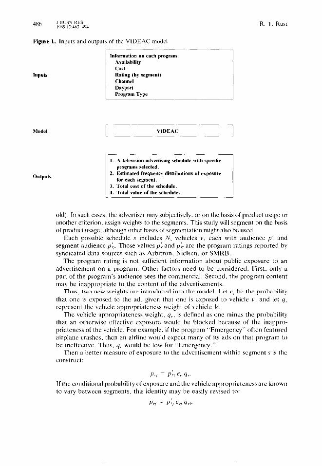
The VIDEAC model, introduced in this study, is designed to help an advertiser select a network television advertising schedule but requires only readily available data. The inputs and outputs of the model are summarized in Figure 1. The inputs are straightforward and require virtually no transformation of data.

During the time period under consideration (perhaps a week, a month, or a quarter) there is a large number of vehicles (programs) on which the advertiser may advertise. Let V denote the set of all these vehicles, and let the number of vehicles in V be N,.. Because each vehicle may be either chosen or not, the number of possible schedules is 2Nl, which is a very large number for even moderate values of N,. Let S denote the set of all possible schedules.

The population is divided into / distinct market segments. The potential sales responses of these moments is, in general, different and will be denoted w, for each segment j. An excellent discussion of several media weights is presented by Gensch [lo]. This weight, w,, is a number chosen by the advertiser to indicate how important he feels segment j is. For example, if segment 1 is considered twice as important as segment 2, the advertiser might set w, = 2 and w2 = 1. Possible criteria that might be used in assigning these weights include brand sales, product sales, or disposable income. Whichever criteria are used, the weight w, serves to emphasize the most important segments in the advertising schedule.

In many cases, the advertiser will specify the segments that are to be considered. These will typically be expressed in terms of demographics (e.g., single women, 18-25 years

4X6 J BUSN RES lvx5:l3:4x3-494

Figure 1. Inputs and outputs of the VIDEAC model

Inputs

Model

Information on each program Availability cost Rating (by segment) Channel Daypart Program Type

1. A television advertising schedule with specific

outputs 2. Estimated frequency distributions of exposure

R. T. Rust

old). In such cases, the advertiser may subjectively, or on the basis of product usage or another criterion, assign weights to the segments. This study will segment on the basis of product usage. although other bases of segmentation might also be used.

Each possible schedule s includes N, vehicles V, each with audience p:. and segment audience p:.,. These values p:. and pii are the program ratings reported by syndicated data sources such as Arbitron, Nielsen, or SMRB.

The program rating is not sufficient information about public exposure to an advertisement on a program. Other factors need to be considered. First, only a part of the program’s audience sees the commercial. Second, the program content may be inappropriate to the content of the advcrtisemcnts.

Thus, two new weights are introduced into the model. Let e, be the probability that one is exposed to the ad, given that one is exposed to vehicle v. and let q, represent the vehicle appropriateness weight of vehicle V.

The vehicle appropriateness weight, q, , is defined as one minus the probability that an otherwise effective exposure would be blocked because of the inappro- priateness of the vehicle. For example, if the program “Emergency” often featured airplane crashes, then an airline would expect many of its ads on that program to be ineffective. Thus. 9, would be low for “Emergency.”

Then a better measure of exposure to the advertisement within segments is the construct:

p,., = P:, e,. 4,..

If the conditional probability of exposure and the vehicle appropriateness are known to vary between segments, this identity may be easily revised to:

PI,, = Pii e,., 4,,.

SELECTING NETWORK ADVERTISING J BUSN RES IYXS: 13:4x3-494 487

Exposure Estimation

In order to determine the comparative value of a schedule, one must first determine the frequency distribution of exposure for that schedule. Also, because the segments are differentially weighted, a frequency distribution of exposure must be estimated for each segment. The exposure estimation method used in the VIDEAC model is the beta binomial distribution (BBD) method, first used for television schedule estimation by Headen, Klompmaker, and Tee1 [12, 131. A detailed description of the exposure estimation method used by VIDEAC, along with empirical tests, have appeared elsewhere [20].

In VIDEAC, a BBD is estimated within each segment. We have, with x as the number of exposures:

where

f,,(x / N,, ~"0) = ($, p”’ (1 - p*)‘“s ’

P(J’ / u.h) = {I‘(u + h) / [l’(U)l‘(h)]~“’ ’ (1 -,y ‘}.

The VIDEAC model thus assumes that every individual has a probability p” that describes that person’s tendency to view the advertising schedule. If there are N programs in the schedule, the probability for that individual to be exposed to k of the N is thus assumed to be B(k, N, p*). Note that this assumes that exposure to a schedule of N programs may be modeled as exposures to N insertions of a “typical” or “average” composite program. This assumption reduces computation considerably, without much loss of fit [25]. This makes it an especially appropriate assumption for modeling network television.

The beta distribution serves as a probability density function for the probability of exposure to any spot in a particular advertising schedule. Because these prob- abilities are allowed to vary across individuals, heterogeneous viewing habits within segments are accounted for. The parameters of the beta are easily obtained from the mean and variance by solving the simultaneous equations that relate the mean and variance to the beta parameters.

The parameters of the beta, for segment j and schedule S, are estimated as follows:

d = {F 1 Ml - P) - v*1> Ml - F) - I.41 - P) - v*1 =k v*//J(1 - CL) - v*

6 = ci(1 - t_L) / /.L,

where

488 J BUSN RES lYXS:l3:4X3-4Y4

R. T. Rust

and

V* = A( 1 + X,)Bl(l + X,)B2 (I + X,)B3 (1 + X,)B4 X,BS X,B6 X,B7 e”.

X, = proportion of same-channel pairs; X, = proportion of same-daypart pairs (“daypart” is time of day. e.g.. “prime

time” evening hours); X3 = proportion of same-program-type pairs; X, = proportion of self-pairs; X, = average effective exposure within the segment; X, = variance of the effective exposure proportions over the vehicles in the

schedule; and X, = N, = number of spots in the schedule. From these parameter estimates, along with the number of vehicles, N,, one

may estimate the frequency distribution of exposure, f,,(x), using the BBD. As formulated here, the VIDEAC model is restricted to estimating exposure to

network television advertising schedules. This restriction may, however, be relaxed. Magazine schedules may be evaluated by substituting the Dirichlet multinomial distribution [5, 151 for the beta binomial model. Mixed television-magazine sched- ules might also be evaluated using a Dirichlet model [21].

Model Formulation

with,

A, Bl, , 87 are coefficients; u is the disturbance term;

Once the frequency distributions of exposure are estimated for a schedule s and each segment j, the total value of schedule s may calculated, using a response function and the segment weights:

TV(s) = 2, W, C;: , f,, (x) R,(x).

This TV function is the objective function to be maximized. In many cases, an empirically derived response function may not be available. In that case, the ad- vertiser may subjectively choose a response function that best represents the re- sponse to the advertising.

The VIDEAC Search Heuristics

The VIDEAC model uses two search heuristics in sequence. The first heuristic, the “greedy” heuristic, adds vehicles one at a time to form an initial schedule. The second heuristic, the “switch” heuristic, tries to improve the value of the schedule by switching vehicles into and out of the initial schedule.

The first heuristic adds vehicles one at a time until the budget constraint is met. It is called “greedy,” because at every step it selects the vehicle that maximizes the per-cost change in the objective function.

In the context of the warehouse location problem, this heuristic has been dis-

SELECTING NETWORK ADVERTISING J BUSN RES 19x5: 13:4x3-4Y4

cussed by Kuehn and Hamburger [14] and others. In an equivalent context, Cor- nuejols, Fisher, and Nemhauser [7] showed that even under worst possible conditions, the heuristic performs well. Because the addition of an advertising vehicle is nearly analogous to the addition of a warehouse, one would expect this heuristic to produce a good initial schedule.

At the start there are no vehicles in the schedule. Then the objective function value is estimated for each one-vehicle schedule. This value is then divided by the vehicle’s cost. The vehicle with the highest per-cost objective function is added to the schedule.

Vehicles are then added one by one until the budget constraint prevents further additions. At each step, per-cost change in the objective function is calculated for those vehicles that will not cause total cost to exceed the budget. The vehicle with the highest per-cost objective function increment is added.

Incremental gain in the objective function for any vehicle interacts strongly with the characteristics of the vehicles already in the schedule. Thus, the ranking of the vehicles typically changes with each step.

The heuristic produces an advertising schedule that is used as a starting schedule for the switch heuristic, which is discussed next.

The switch heuristic begins with the initial schedule produced by the “greedy” heuristic. It then seeks to increase the objective function by switching vehicles into and out of the schedule. This kind of heuristic, as well as its use in combination with a “greedy” heuristic, is discussed by Kuehn and Hamburger [14].

The heuristic begins by ranking all of the available vehicles in order of weighted cost per thousand, which is proportional to

weighted cost per impression = c, i (Z,w, p,,),

where w, is the segment weight for segment j, p,., is the effective rating of vehicle v in segment i, and c, is the cost of vehicle v.

The heuristic then removes from the schedule (on a trial basis) the vehicle that was added latest. It then attempts to replace it with each of the available vehicles, in order of weighted cost per thousand. Whenever a vehicle is found that improves the objective function, that vehicle is added to the schedule, and the vehicle that had been removed on trial is actually removed. Occasionally this will result in a vehicle being removed from the schedule and then restored to the schedule later on, due to interaction with other vehicles that have been added.

When a trial removal cannot be replaced with profit by any of the outside vehicles, the next most recently added vehicle becomes the vehicle that is removed from the schedule on trial.

The switching goes on until none of the vehicles in the schedule may be profitably replaced by an outside vehicle. That schedule is the schedule that is selected by the VIDEAC model.

Operationalization of the Model

The Data

The data were provided by SMRB (formerly W. R. Simmons & Associates Re- search, Inc.), and are from their 1977/78 report [22, 231. The SMRB respondents

490 J BUSN RES lYxs:l3:4x3-4Y1 R. T. Rust

were selected using a multistage area cluster sample. Television data were collected from 5652 respondents in a six-week period from October 9 to November 19, 1977. The 5652 respondents represent a subsample of 15,003 original respondents, all of whom answered questionnaires concerning demographics, product usage, and use of other media.

Each of the 5652 respondents completed a television diary in which they re- corded, for each half-hour interval, the programs they viewed. These diaries were kept for two consecutive weeks. Each respondent was at least 18 years old. and no two respondents were from the same household.

Illustration

The VIDEAC model was used to select a hypothetical network television adver- tising schedule for an actual product.

The product chosen for the test was a convenience-oriented service. The Sim- mons data contain each respondent’s self-reported figure of the number of times he or she used the service in the last month.

Two market segments were used: heavy users and light users. Heavy users were defined as those who said they used the service eight times or more in the last month.

Several aspects of the model needed to be specified before a schedule could be selected. These aspects included segment weights, vehicle appropriateness, choice of response function, the availability of vehicles, vehicle cost, budget, and sched- uling period.

Segment weights were computed on the basis of average product usage times size of segment. The heavy-user segment was smaller, but it was worth much more per capita.

Conditional probability of exposure and vehicle appropriateness were deleted from the formulation because of lack of information.

The response function chosen was

R(x) = P.

In this case, response refers to only the controllable response. Some response is likely to occur, even if there is no advertising, but this response is by definition unaffected by advertising. The particular functional form was chosen on the basis of an empirical study performed on data collected for a major consumer goods company [19]. In order to simulate the unavailability of vehicles. some of the vehicles were randomly declared unavailable.

Vehicle cost was estimated on the basis of rating, daypart. and average daypart cost per thousand for each network. Average daypart costs per thousand for each network were computed from each network’s average daypart rating and average daypart cost. Average daypart rating was calculated from the SMRB data, and average daypart cost was obtained from the Standard Rate and Data Service. The costs quoted there are overestimates but are adequate for the purposes of this study (an actual advertiser will have more accurate cost data). In recognition of the fact that most higher-rated shows demand a higher cost per thousand, a rating- based cost adjustment was made.

SELECTING NETWORK ADVERTISING

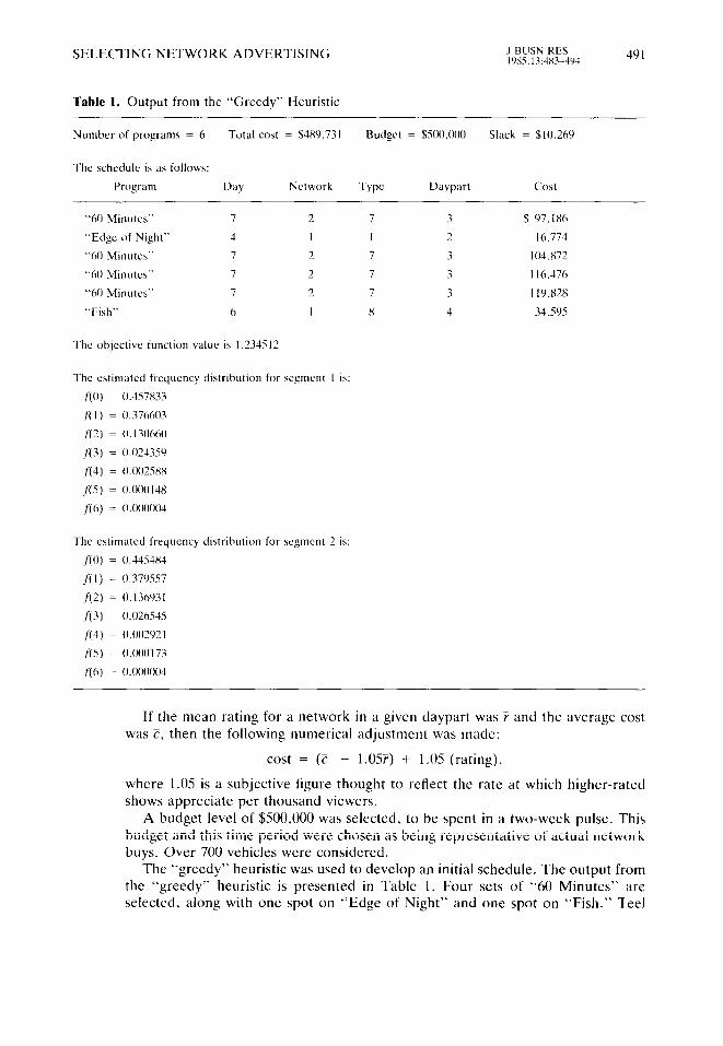
Table 1. Output from the “Greedy” Heuristic

J BUSN KES lYXS:13:4X3-4Y4 491

Number of programs = 6 Total cost = $489.731 Budget = $SOO.OOO Slack = $10.269

The schedule is as follows:

Program Day Network Type Daypart Cost

“60 Minutes” 7 2 7 3 $ 97.1X6

“Edge of Night” 4 1 I 2 16.774

“60 Minutes” 7 2 7 3 104,872

“60 Minutes” 7 2 7 3 116.476

“60 Minutes” 7 2 7 3 I19.82X

“Fish” 6 I x 4 34.595

The objective function value is 1.234.5 I2

The estimated frequency distribution for segment I is:

fl0) = 0.457833

f(I) = 0.376603

.fl2) = 0.1306hO

l(3) = 0.024359

j(4) = 0.0025xx

.flS) = 0.000148

f16) = 0.000004

The estimated frequency distribution for segment 2 is:

fl0) = 0.44S384

fl I) = 0.379557

f(2) = 0.136931

,f(3) = 0.026S4S

f(4) = 0.002021

J7S) = 0.000173

flcl) = 0.000004

If the mean rating for a network in a given daypart was ? and the average cost was C, then the following numerical adjustment was made:

cost = (C - 1.0%) + 1.05 (rating).

where 1.05 is a subjective figure thought to reflect the rate at which higher-rated shows appreciate per thousand viewers.

A budget level of $500,000 was selected, to be spent in a two-week pulse. This budget and this time period were chosen as being representative of actual network buys. Over 700 vehicles were considered.

The “greedy” heuristic was used to develop an initial schedule. The output from the “greedy” heuristic is presented in Table 1. Four sets of “60 Minutes” are selected, along with one spot on “Edge of Night” and one spot on “Fish.” Tee1

492 J BUSN KES lY8S:l3:183-4~J4

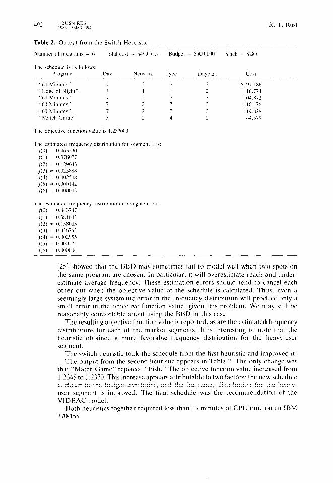
Table 2. Output from the Switch Heuristic

R. T. Rust

Number of programs = 6 Total cost = $-1YY.715 Budget = $500.000 Slack = $25

The schedule is as follows:

Program Day Network Type Daypurt Cost

“60 Minutes” 7 7 7 3 $ 97.1X6

“Edge of Night” 4 I I 2 16.771

“60 Minutes” 7 2 I 3 IOJ.X72

“60 Minutes” 7 2 7 3 116.476

“60 Minutes” 7 2 7 3 110.x2x “Match Game” 5 2. 4 7 41.57Y

The ohjcctive function value is I .237000

The atimated frequcnq distribution for scemcnt I is: f(O) = 0.463330 f(l) = 0.378077

f(7) = 0.12Y643

fl.?) = 0.0238X8

fl4) = 0.002508

t‘(5) = 0.000142

.flh) = 0.000003

The estimated frequency distribution tar wgment 2 i’r:

JO) = 0.443737

.fl I) = 0.3x1033

fl?) = 0.13x00.5

f73) = 0.026753

114) = 0.007Y55

1’(5) = 0.000175

f(6) = o.ooooo‘l

[25] showed that the BBD may sometimes fail to model well when two spots on the same program arc chosen. In particular. it will overestimate reach and under- estimate average frequency. These estimation errors should tend to cancel each other out when the objective value of the schedule is calculated. Thus. even a seemingly large systematic error in the frequency distribution will produce only a small error in the objective function value. given this problem. WC may still be reasonably comfortable about using the BBD in this case.

The resulting objective function value is reported, as are the estimated frequency distributions for each of the market segments. It is interesting to note that the heuristic obtained a more favorable frequency distribution for the heavy-user segment.

The switch heuristic took the schedule from the first heuristic and improved it. The output from the second heuristic appears in Table 2. The only change was

that “Match Game” replaced “Fish.” The objective function value increased from 1.2345 to 1.2370. This increase appears attributable to two factors: the new schedule is closer to the budget constraint, and the frequency distribution for the heavy- user segment is improved. The final schedule was the recommendation of the VIDEAC model.

Both heuristics together required less than 13 minutes of CPU time on an IBM

3701155.

SELECTING NETWORK ADVERTISING J BUSN RES 19x.5: 13:4833-4Y4 4Y3

Summary

The VIDEAC model is a quick, economical, and efficient model for selecting

network television advertising schedules. It incorporates an improved frequency distribution estimation procedure and is flexible enough to permit (but not require) many empirical and subjective inputs.

It is an improvement over currently published models for the selection of network television advertising schedules and may be extended to accommodate other media or mixed-media schedules.

References

1.

2.

3 _

4.

5.

6.

7.

8.

9.

10.

11.

12.

13.

14.

15.

16.

17.

Aaker, David A., ADMOD: An Advertising Decision Model, Journal of Marketing Research 12 (February 1975): 37-45.

Bass, Frank M.. and Lonsdale, Ronald T., An Exploration of Linear Programming in Media Selection, Journal of Murketing Research 3 (May lY66): 179-188.

Broadbent, Simon R.. A Year’s Experience of the LPA Media Model, ARF 11th Annuul Conference Proceedings (October 1965): 51-56.

Brown, Douglas B., and Warshaw, Martin R., Media Selection by Linear Programming. Journal of Murketing Research 2 (February 1965): 83-88.

Chandon. Jean-Louis Jose, A Comparative Study of Media Exposure Models, unpublished Ph.D. dissertation, Northwestern University, Chicago, 1076.

Charnes. Cooper, Lerner, DeVoe. and Reinecke, A Goal Programming Model for Media Planning, Management Science 14 (April 1968): 423-430.

Cornuejols, Gerard, Fisher, Marshall L., and Nemhauser. George L., Location of Bank Accounts to Optimize Float: An Analytic Study of Exact and Approximate Algorithms, Management Science 23 (April 1977): 7X9-810.

Dunn, S. Watson, and Barban. Arnold M.. Advertising: Its Role in Modern Marketing. 4th ed. Hinsdale, Ill., Dryden Press. 1978.

Gensch. Dennis H., A Computer Simulation Model for Selecting Advertising Schedules, Journul of Marketing Reseurch 6 (May 1969): 203-214.

~ Media Factors: A Review Article, Journal of Marketing Research 7 (May 1970): 216-22;.

Advertising Planning: Muthemuticul Models in Advertising Media Planning. Amsteidam: Elsevier Scientific Publishing Company, 1973.

Headen, Robert S., Klompmaker. Jay E.. and Teel. Jesse E.. Jr.. Predicting Audience Exposure to Spot TV Advertising Sch&ules, Journal of Marketing Research 14 (February 1977): 1-Y.

-, Predicting Network TV Viewing Patterns, Journal of Advertising Research 19 (August 1979): 49-54.

Kuehn, A.A.. and Hamburger, M.J.. A Heuristic Program for Locating Warehouses. Management Science 9 (1963): 643-666.

Leckenby, John D., and Kishi, Shizue, The Dirichlet Multinomial Distribution as a Magazine Exposure Model. Journal of Marketing Reseurch 21 (February 1984): lOO- 106.

Little, John D.C., and Lodish, Leonard M., A Media Selection Model and Its Optimization by Dynamic Programming, Industrial Management Review 8 (Fall 1966): 15-24.

- A Media Planning Calculus. Operations Research 17 (January-February 1969): l-35. ’

494 J HUSN RES IOX5: 13:183-493

R. T. Rust

IX.

19.

20.

21.

22.

23.

24.

2s.

26.

27.

Moran. William T.. Practical Media Models-What Must They Look Like?, ARF 8th Annuul Conference Proceedings (October IY62): 30-38.

Rust, Roland T.. A Model for the Selection of Television Advertising Schedules. unpublished Ph.D. dissertation, Chapel Hill. University of North Carolina. 1070.

Rust, Roland T.. and Klompmaker. Jay E.. Improving the Estimation Procedure for the Beta Binomial TV Exposure Model, Journul o,f Murketing Reseurch I8 (November 19X1): 442-448.

Rust, Roland T., and Leone, Robert P.. The Mixed-Media Dirichlet Multinomial Distribution: A Model for Evaluating Television-Magazine Advertising Schedules, Jourrwl

qf Marketiq Research 21 (February 1984): 8Y-YY.

Simmons Media Studies, Selective Murkets and the Media Rruchin~ Tlzem. Simmons Media Studies. New York, 1078.

__ Technicul Guide: 1977178 St&v of Selective Murkets and the Mediu Reaching Them. ‘Simmons Media Studies. New York. lY7X.

Stasch. Stanley F.. Linear Programming and Space-Time Considerations in Media Selection. Journd of Advertising Reseurch 5 (December lY65): 40-46.

Teel, Jesse E., Jr., Modeling Audience Exposure to Network TV Advertising Schedules. unpublished Ph.D dissertation. Chapel Hill, University of North Carolina. lY76.

Wilson. Clark L.. and Maneloveg, Herbert. A Year of LP Media Planning for Clients. ARF Midwest C’onftJrence (November lY62): 7X-8Y.

Zangwill, Willard I.. Media Selection by Decision Programming, Jowxal of Advertising Research 5 (September 1965): X-36.