Selection on an Index of Traits I= X b j z j =b T z æ 2 I =æ(b T z;b T z)=b T æ(z;z)b=b T Pbæ 2 A I =æ A (b T z;b T z)=b T æ A (z;z)b=b T Gb h 2 I = æ

Selection on an Index of Traits

I =X

bjzj = bT z

æ2I =æ(bT z;bT z) = bTæ(z;z)b = bT Pb

æ2A I =æA(bT z;bT z) = bTæA(z;z)b = bT Gb

h2I =

æ2A I

æ2I

= bT GbbT Pb

A common way to select on a number of traits at onceis to base selection decisions on a simple index oftrait values,

The resulting phenotypic and additive-genetic variancefor this synthetic trait are;

This gives the resulting heritability of the index as

Class problem

Enter G and P matrices from Example 33.1 in R.

For QuickTime™ and aTIFF (LZW) decompressor

are needed to see this picture.

Compute additive and phenotypic variance, andh2 for the index

R I ={h2I æI ={¢

bT Gb

bT Pb

pbT Pb ={¢

bT Gbp

bT Pb

Sj ={

æI

X

k

bkP j k S ={

æIPb

Thus, the response in the index due to selection is

How does selection on I translate into selection onthe underlying traits?

Since R = GP-1S, the response vector for theunderlying means becomesR = GP ° 1S =

{æI

Gb ={¢Gb

pbT Pb

-

Class problem

For a selection intensity of i = 2.06 (upper 5% selected)compute the response in the index and the vectors ofselection differentials and responses (S and R)for the vector of traits.

Changes in the additive variance of the index

QuickTime™ and aTIFF (LZW) decompressor




Bulmer’s equation holds for the index:

We can also apply multivariate Bulmer to follow thechanges in the variance-covariance matrix of thecomponents:



The Smith-Hazel IndexSuppose we wish the maximize the response on thelinear combination aTz of traits



This is done by selecting those individuals withthe largest breeding value for this index, namely

Hence, we wish to find a phenotypic index I = bTzSo that the correlation between H and I in anIndividual is maximized.

Key: This vector of weights b is typically rather different from a!



The Smith-Hazel Index



Smith and Hazel show that the maximal gain is obtainedby selection on the index bTz where

Thus, to maximize the response in aTz in the nextgeneration, we choose those parents with thelargest breeding value for this trait, H = aTg. Thisis done by choosing individuals with the largestvalues of I = bs

Tz.

In-class problem

We wish to improve the index QuickTime™ and aTIFF (LZW) decompressor


Compute the Smith-Hazel weights (using previousP, G)

Compute the response for the SH index with truncationselection saving the upper 5%

Compare this response to that selecting directly on I=aTz

Heritability index : bi = a ih2i

Other indices


are needed to see this picture.Estimated index:


are needed to see this picture.Base-index:

Elston (or weight-free) index:



Retrospective index: since R = Gb, b = G-1R

Problem with Smith-Hazel

Require accurate estimate of P, G!

Values of P, G change each generation from LD!

Dealing with negative eigenvalues of H = P-1G

Bending:QuickTime™ and a

TIFF (LZW) decompressorare needed to see this picture.

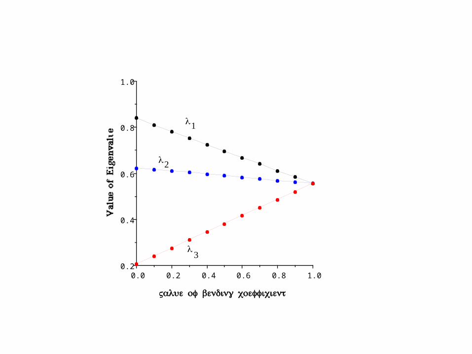
1.00.80.60.40.20.00.2

0.4

0.6

0.8

1.0

Value of Eigenvalue

λ

λ

λ

Value of bending coefficient

1

2

3

Restricted and Desired-gains Indices

Instead of maximizing the response on a index, wemay (additionally) wish to restrict change in certaintraits or have a desired gain in specific traits in mind

Suppose for our soybean bean data, we wish no response in trait 1

Class Problem: Suppose weights are aT = (0,1,1), i.e,no weight on trait 1. Compute the response in traitone under this index.

Morely (1955): Change trait z1 while z2 constant







Want b1, b2 such thatno response in trait 2

Setting b1 = 1 and solving gives weights



Note sign typo inEquation 33.36

Kempthorne-Nordskog restricted index

Suppose we wish the first k traits to be unchanged.

Since response of an index is proportional to Gb,the constraint is CGbr =0, where C is an m X k matrixwith ones on the diagonals and zeros elsewhere.



Kempthorne-Nordskog showed that br is obtained by

where Gr = CG





Tallis restriction index



More generally, suppose we specify the desiredgains for k combinations of traits,

Here the constraint is CR = CGbr = d



Solution is

Desired-gain indices

Suppose we desire a gain of R, then since R = Gb,

The desired-gains index is b = G-1R







Class problem

Compute b for desired gains (in our soybean traits)of (1,-2,0)

Non-linear indices



Care is required in considering the improvement goals when using a nonlinear merit function, as apparently subtle differences in the desired outcomes can become critical

A related concern is whether we wish to maximize the additive Genetic value in merit in the parents or in their offspring. Again, with a linear index these are equivalent, as the mean breeding value of theparents u equals the mean value in their offspring.This is not the case with nonlinear merit.

Quadratic selection index









Linearization



Fitting the best linear index to a nonlinearmerit function









Sets of response vectors and selection differentials



Given a fixed selection intensity i, we would like toknow the set of possible R (response vectors) orS (selection vectors)




are needed to see this picture.Substituting the above value of b into

recovers


are needed to see this picture.Hence,

This equation describes a quadratic surface ofpossible, R values,




are needed to see this picture.Similarly,



Key: Optimal weights a function of intensity of selectionQuickTime™ and aTIFF (LZW) decompressor


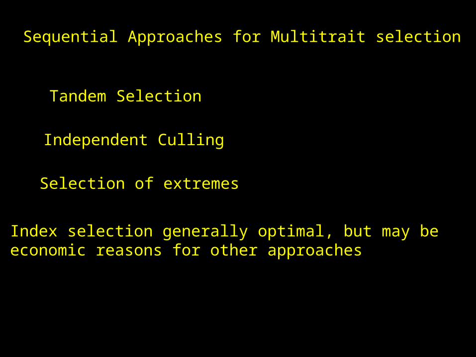
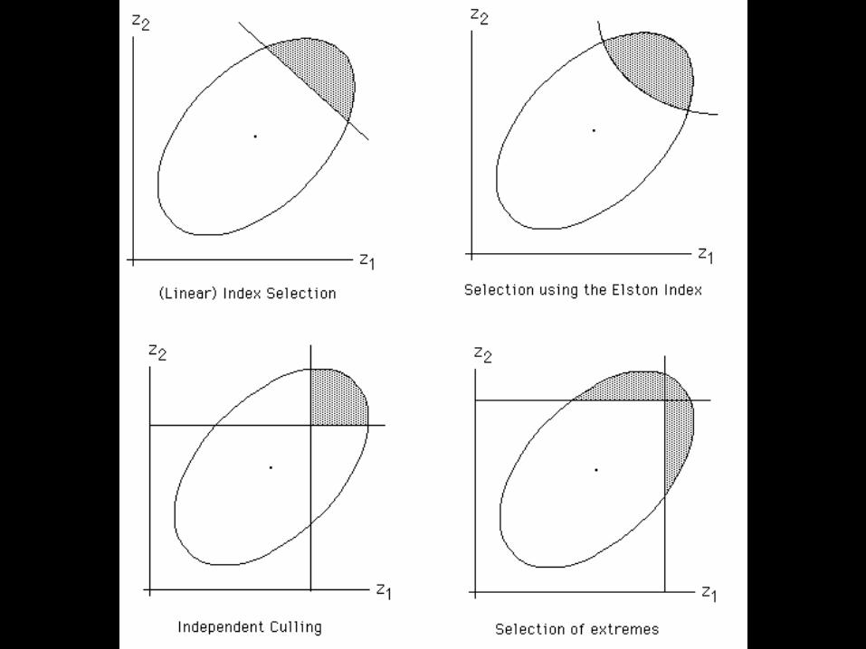
Sequential Approaches for Multitrait selection

Tandem Selection

Independent Culling

Selection of extremes

Index selection generally optimal, but may beeconomic reasons for other approaches

Multistage selectionSelecting on traits that appear in different lifestages

Optimal selection schemes

Cotterill and James optimal 2-stage. Select 1st on x,(save p1), then then on y (save p2 = p/p1). Goaloptimize the breeding value for merit g.



Documents

Selection on an Index of Traits I= X b j z j =b T z æ 2 I =æ(b T z;b T z)=b T æ(z;z)b=b T Pbæ 2 A I =æ A (b T z;b T z)=b T æ A (z;z)b=b T Gb h 2 I = æ