Self-Supporting Rhombic Infill Structures for Additive Manufacturing

Jun Wu*1,4, Charlie C.L. Wang2,3, Xiaoting Zhang3, and Rudiger Westermann4

1Department of Mechanical Engineering, Technical University of Denmark, Denmark

2Department of Design Engineering, Delft University of Technology, The Netherlands

3Department of Mechanical and Automation Engineering, The Chinese University of Hong Kong, P. R. China

4Department of Informatics, Technische Universitat Munchen, Germany

*Corresponding Author. Tel: +45 4525 4255. Fax: +45 4525 1961. Email: junwu@mek.dtu.dk

Abstract

Recent work has demonstrated that the interior material layout of a 3D model can be designed to make a fabricated replica satisfyapplication-specific demands on its physical properties, such as resistance to external loads. A widely used practice to fabricate suchmodels is by layer-based additive manufacturing (AM), which however suffers from the problem of adding and removing interiorsupporting structures. In this paper, we present a novel method for generating application-specific infill structures on rhombiccells so that the resultant structures can automatically satisfy manufacturing requirements on overhang-angle and wall-thickness.Additional supporting structures can be avoided entirely in our framework. To achieve this, we introduce the usage of an adaptiverhombic grid, which is built from an input surface model. Starting from the initial sparse set of rhombic cells, via numericaloptimization techniques an objective function can be improved by adaptively subdividing the rhombic grid and thus adding morewalls in cells. We demonstrate the effectiveness of our method for generating interior designs in the applications of improvingmechanical stiffness and static stability.

Keywords: infill, self-supporting, geometric algorithm, optimization, additive manufacturing

1. Introduction

The shape of 3D models can be designed by a variety of ge-ometric modeling tools. To create a physical replica of suchshapes, instead of manufacturing the object with a solid inte-rior, a typical practice in AM is to use a uniform infill with anadjustable percentage of voids. The purpose is to balance themechanical quality and the cost associated with material con-sumption and fabrication time. To serve specific purposes suchas load bearing [1] or standing [2], a number of studies havebeen devoted to the generation of optimized interior.

However, in many (if not all) cases, the optimized structurescannot be directly fabricated by layer-based AM. Specifically, ifthe shapes have a relatively large overhang, the manufacturingmaterial cannot be deposited on a layer where there is no mate-rial below it. Recent developments in AM address this problemby automatically generating support structures below the layerswith overhang (e.g., [3, 4, 5]).

A support structure can be fabricated by either a dissolvablematerial or the same material as the main body. If a dissolvablematerial is employed, exterior supports can be removed auto-matically in a post-process (ref. [6]). The removal procedurehas to be performed manually if single-material manufactur-ing is employed (e.g., SLA and the low-cost FDM machines1).

1SLA and FDM stands for Stereolithography Apparatus and Fused Deposi-tion Modeling, which are two widely used approaches in AM.

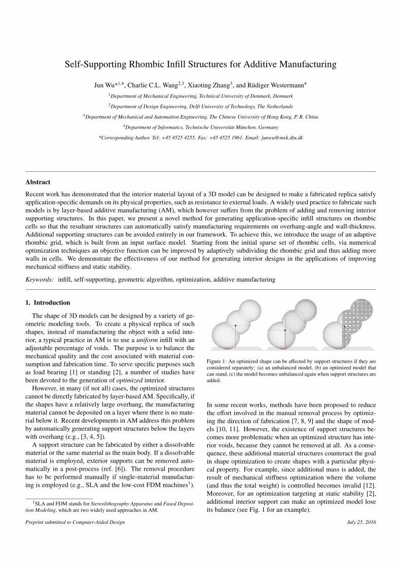
Figure 1: An optimized shape can be affected by support structures if they areconsidered separately: (a) an unbalanced model, (b) an optimized model thatcan stand, (c) the model becomes unbalanced again when support structures areadded.

In some recent works, methods have been proposed to reducethe effort involved in the manual removal process by optimiz-ing the direction of fabrication [7, 8, 9] and the shape of mod-els [10, 11]. However, the existence of support structures be-comes more problematic when an optimized structure has inte-rior voids, because they cannot be removed at all. As a conse-quence, these additional material structures counteract the goalin shape optimization to create shapes with a particular physi-cal property. For example, since additional mass is added, theresult of mechanical stiffness optimization where the volume(and thus the total weight) is controlled becomes invalid [12].Moreover, for an optimization targeting at static stability [2],additional interior support can make an optimized model loseits balance (see Fig. 1 for an example).

Preprint submitted to Computer-Aided Design July 25, 2016

Therefore, the effect of support structures must be consideredsimultaneously in the optimization process, or the need for suchstructures must be avoided entirely, for instance, by limitingthe maximum allowed overhang during topology optimization(ref. [13]). This approach, however, cannot completely ensurethat no overhang is generated. Moreover, adding the respectiveconstraints into the optimization process increases the problemcomplexity and deteriorates the convergence of the employednumerical simulation schemes.

To overcome the aforementioned problem in interior struc-ture optimization, we present a new method for infill optimiza-tion that ensures the resultant structures are self-supporting. Astructure is said to be self-supporting if its surfaces have anoverhang-angle smaller than a prescribed maximum overhang-angle, and thus the structure can be fabricated without addingsupports below all its surfaces. Our method restricts the com-putational domain to a special class of spaces which are self-supporting and let control the size of the smallest features.Specifically, we advocate the use of rhombic cell structuresas composites of the interior, where the maximum overhang-angle and the minimum wall-thickness can be specified explic-itly. With these composites, we carry out an optimization pro-cess to gradually update the interior structures of a given modeltowards different specific usages, at the same time enforcingmanufacturability of the results. The specific contributions ofour work are as follows:

• We account for manufacturability explicitly by restrictingtopology optimization to generate structures living in amanufacturability-ensured space, i.e., represented by a hi-erarchical grid of rhombuses.

• We demonstrate the use of grid refinement and cell-to-shell operators to efficiently perform the optimization pro-cess.

• We demonstrate the effectiveness of our approach for theoptimization of mechanical stiffness and static stability.

To the best of our knowledge, our proposed approach is thefirst that can ensure the manufacturability (i.e., bounds of themaximum overhang-angle and the minimum wall-thickness) ofoptimized interior structures.

The remainder of this paper is organized as follows. Afterreviewing work that is related to ours in Section 2, the overallmethodology of our infill optimization framework is introducedin Section 3. The use of adaptive rhombic structures as the com-putational domain is discussed in Section 4. The formulationfor optimizing the mechanical stiffness and the static stabilityis given in Section 5 to exemplify the use of our method. Re-sults are shown in Section 6 to verify the effectiveness of ourapproach.

2. Related Work

With the development of additive manufacturing techniquesin recent years, more and more research has been devoted to

geometric and physical modeling for AM (also called 3D print-ing). The purpose of this section is to discuss the strengths andlimitations of approaches most closely related to ours, ratherthan providing a comprehensive survey. For the latter, let usrefer to [14, 15].

Interior Shape Optimization The interior structure of amodel can be optimized to meet different objectives on physicalproperties. The static balance has been considered in [2, 16],which is later extended to dynamic balance [17] by changingboth the surface of an input model and its interior infills. Tar-geting a variety of stability objectives, Musialski et al. [18] op-timize the interior by proposing a reduced-order parametriza-tion of offset surfaces. Wu et al. [19] present an analysis ofthe optimal topology regarding static and rotational stability,and propose a reduced yet accurate optimization based on ray-reps. A heuristic method is developed in [20] to construct meso-structure inside a model to change its mechanical property. Askin-frame structure is optimized in [21] for enhancing the me-chanical stiffness of objects fabricated by 3D printing. Lu etal. [1] compute the interior structure for a similar purpose butuse different structures – honeycomb-cells. Among all theseapproaches, except [16] which fills the interior void by pre-defined regular patterns, interior structures generated via op-timization faces the problem of large overhangs. As a result,the interior structure cannot be fabricated directly without sup-port structures. We tackle this problem by using self-supportingrhombic structures in the optimization process.

Support Structures during 3D Printing Adding supports toa model leads to the problems of material waste, longer fabri-cation time and lower surface quality. Approaches have beendeveloped to reduce the usage of support structure to resolvethese problems. For example, an optimal printing direction issearched in [4] according to the total area of facing down re-gions (i.e., places where support structures need to be added).As a result, the total volume of the used support structure and,thus, additional material cost can be reduced. In the recent workof Zhang et al. [8], a perceptual model is developed using atraining-and-learning strategy to consider multiple influencesthat will be given on a fabricated model by support structures.The best printing directions are determined by composing allthe factors including contact area, visual saliency, viewpointpreference, and smoothness entropy. Given a fixed printing di-rection, the shape of an input model is optimized in [10, 11]to reduce the area of facing down regions so that less supportstructures are needed. Some approaches consider another as-pect of supports – the stability. Unlike the tree structures usedin [4, 8], bridge structures are suggested in [3, 5, 22]. Differentfrom such techniques for reducing the usage of external sup-ports, we optimize interior structures with the goal to ensurethat they are self-supporting and thus can completely eliminatethe usage of additional interior supports.

Topology Optimization Topology optimization has beenwidely used for product and structure design, and very compactcode has been developed for well-posed problems (e.g., [23]).Recently, Wu et al. [24] have developed a high-throughput sys-

2

tem to improve the efficiency of topology optimization on 3Dsolids. Unlike the prior method which computes optimizedshape and topology on a fixed structure of grids, Wang etal. [12] represent the structural boundary by a level-set modelthat is embedded in a scalar function of a higher dimension. Theparametric control is realized in [25] by presenting level-sets ofa higher-dimensional function derived from B-splines and com-bining primitives with R-functions. Different representationshave been developed to control the domain of computation, in-cluding the B-spline space [26], the medial zone [27], and thedynamically changed simplicial complex [28]. Our research isrelated to these works in the sense that we follow the idea ofrestricting the computational domain to fully control geometricfeatures. In particular, our framework computes on an adap-tive rhombic grid to ensure the manufacturability constraintsincluding self-support and a minimum thickness constraint forwall structures.

Self-Supporting Structures In computer graphics, the term”self-supporting” has been used in related-but-different con-texts other than concerning the overhang-angle. Specifically,self-supporting in architectural geometry refers to structureswhich as a whole stand in static equilibrium without externalsupport. The structure of self-supporting masonry was studiedin [29, 30], and nonlinear optimization was used in [29] to ap-proximate an arbitrary surface by such structures. Instead ofassembling self-supporting structures, Whiting et al. [30] pro-posed an approach to guide the design process so that a self-supporting shape is formed. The self-supporting surface canalso be constructed with the help of regular triangulation asstudied in [31]. The assembly of building blocks to form a self-supporting structure is investigated in [32] to govern the processof construction. Recently, self-supporting shape is computedon parametric surfaces, which is a standard representation offreeform surfaces in CAD systems (ref. [33]). However, onlythe shape of a surface (but not topology) is optimized in mostof these approaches.

3. Methodology

To ensure the manufacturability of infill structures, ourmethod performs the computation using a hierarchical grid rep-resentation. In particular, we develop a tree structure withrhombic cells that is self-supporting and with controlled small-est feature sizes (see Section 4.1). Topology of the tree structurecan be changed using adaptive spatial refinement similar to anoctree, yet it subdivides rhombic cells.

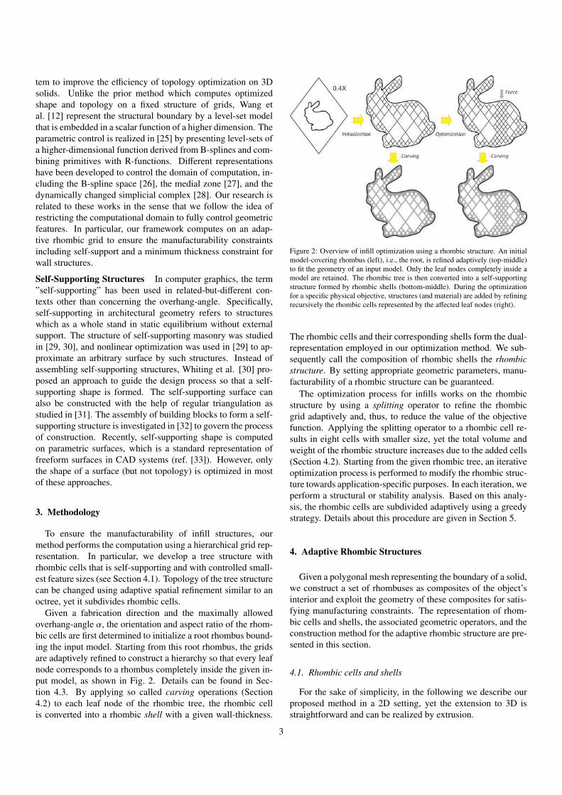
Given a fabrication direction and the maximally allowedoverhang-angle α, the orientation and aspect ratio of the rhom-bic cells are first determined to initialize a root rhombus bound-ing the input model. Starting from this root rhombus, the gridsare adaptively refined to construct a hierarchy so that every leafnode corresponds to a rhombus completely inside the given in-put model, as shown in Fig. 2. Details can be found in Sec-tion 4.3. By applying so called carving operations (Section4.2) to each leaf node of the rhombic tree, the rhombic cellis converted into a rhombic shell with a given wall-thickness.

Figure 2: Overview of infill optimization using a rhombic structure. An initialmodel-covering rhombus (left), i.e., the root, is refined adaptively (top-middle)to fit the geometry of an input model. Only the leaf nodes completely inside amodel are retained. The rhombic tree is then converted into a self-supportingstructure formed by rhombic shells (bottom-middle). During the optimizationfor a specific physical objective, structures (and material) are added by refiningrecursively the rhombic cells represented by the affected leaf nodes (right).

The rhombic cells and their corresponding shells form the dual-representation employed in our optimization method. We sub-sequently call the composition of rhombic shells the rhombicstructure. By setting appropriate geometric parameters, manu-facturability of a rhombic structure can be guaranteed.

The optimization process for infills works on the rhombicstructure by using a splitting operator to refine the rhombicgrid adaptively and, thus, to reduce the value of the objectivefunction. Applying the splitting operator to a rhombic cell re-sults in eight cells with smaller size, yet the total volume andweight of the rhombic structure increases due to the added cells(Section 4.2). Starting from the given rhombic tree, an iterativeoptimization process is performed to modify the rhombic struc-ture towards application-specific purposes. In each iteration, weperform a structural or stability analysis. Based on this analy-sis, the rhombic cells are subdivided adaptively using a greedystrategy. Details about this procedure are given in Section 5.

4. Adaptive Rhombic Structures

Given a polygonal mesh representing the boundary of a solid,we construct a set of rhombuses as composites of the object’sinterior and exploit the geometry of these composites for satis-fying manufacturing constraints. The representation of rhom-bic cells and shells, the associated geometric operators, and theconstruction method for the adaptive rhombic structure are pre-sented in this section.

4.1. Rhombic cells and shells

For the sake of simplicity, in the following we describe ourproposed method in a 2D setting, yet the extension to 3D isstraightforward and can be realized by extrusion.

3

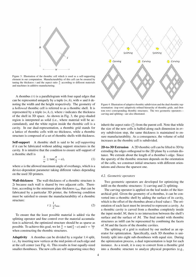
Figure 3: Illustration of the rhombic cell which is used as a self-supportingelement in our computation. Manufacturability of this cell can be ensured bytuning the thickness t and the aspect ratio h

w according to different materialsand machines in additive manufacturing.

A rhombus (♦) is a parallelogram with four equal edges thatcan be represented uniquely by a tuple (w, h), with w and h de-noting the width and the height respectively. The geometry ofa hollowed rhombic cell is referred to as a rhombic shell. It isrepresented by a triple (w, h, t), where t indicates the thicknessof the shell in 3D space. As shown in Fig. 3, the gray-shadedregion is interpreted as solid (i.e., where material will be ac-cumulated), and the white region inside the rhombic cell is acavity. In our dual-representation, a rhombic grid stands fora lattice of rhombic cells with no thickness, while a rhombicstructure is composed of a set of rhombic shells with thickness.

Self-support A rhombic shell is said to be self-supportingif it can be fabricated without adding support structures in thecavity. It is intuitive that the condition to ensure self-support ofa rhombic shell is

hw≥ tan(

π

2− α), (1)

where α is the allowed maximum angle of overhangs, which is adevice-dependent parameter taking different values dependingon the used 3D printers.

Wall-thickness The wall-thickness of a rhombic structure is2t because each wall is shared by two adjacent cells. There-fore, according to the minimum plate thickness tmin that can befabricated by a particular 3D printer, the following conditionmust be satisfied to ensure the manufacturability of a rhombicstructure:

t ≥12

tmin. (2)

To ensure that the least possible material is added via thesplitting operator and fine control over the material accumula-tion is achieved, the optimized structure should be as sparse aspossible. To achieve this goal, we let h

w = tan( π2 −α) and t = tmin2

when constructing the rhombic structures.

Adaptivity A rhombus can be divided by a regular 1:4 split,i.e., by inserting new vertices at the mid points of each edge andat the cell center (see Fig. 4). This results in four equally-sizedsmaller rhombuses. The new cells are self-supporting since they

Figure 4: Illustration of adaptive rhombic subdivision and the dual rhombic rep-resentation: (top row) adaptively refined hierarchy of rhombic grids, and (bot-tom row) corresponding rhombic structures. The two geometric operators—carving and splitting—are also illustrated.

inherit the aspect ratio ( hw ) from the parent cell. Note that while

the size of the new cells is halfed along each dimension in ev-ery subdivision step, the same thickness is maintained to en-sure manufacturability. As a consequence, the volume of solidincreases as the rhombic cell is subdivided.

2D-to-3D Extrusion A 2D rhombic cell can be lifted to 3D byextruding the edges orthogonal to the 2D plane by a certain dis-tance. We extrude about the length of a rhombus’s edge. Sincethe sparsity of the rhombic structure depends on the orientationof the cells, we construct initial structures with different orien-tations and choose the sparsest one.

4.2. Geometric operators

Two geometric operators are developed for optimizing theinfill on the rhombic structures: 1) carving and 2) splitting.

The carving operator is applied on the leaf nodes of the hier-archical grid. Given the geometry of a rhombus, it can be con-verted into a rhombic shell by adding the surface of its cavity,which is the offset of the rhombus about a fixed value t. The ori-entation of each facet must be inverted to represent a cavity. Asa rhombic cavity is carved from a rhombus completely insidethe input modelM, there is no intersection between the shell’ssurface and the surface of M. The final model with rhombicstructures as infill can be represented by combining the facetsofM and the facets of the rhombic cavities.

The splitting of a grid is realized by our method as an op-erator for optimization. Specifically, each 3D rhombus is uni-formly split into eight sub-rhombuses with equal size. Duringthe optimization process, a dual representation is kept for eachinstance. As a result, it is easy to convert from a rhombic gridinto a rhombic structure to analyze physical properties (e.g.,

4

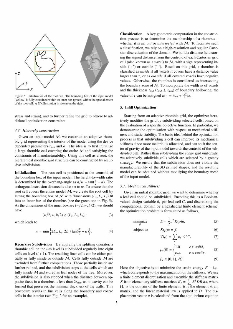
Figure 5: Initialization of the root cell. The bounding box of the input model(yellow) is fully contained within an inner box (green) within the spacial extentof the root cell. A 3D illustration is shown on the right.

stress and strain), and to further refine the grid to adhere to ad-ditional optimization constraints.

4.3. Hierarchy construction

Given an input model M, we construct an adaptive rhom-bic grid representing the interior of the model using the devicedepended parameters tmin and α. The idea is to first initializea large rhombic cell covering the entire M and satisfying theconstraints of manufacturability. Using this cell as a root, thehierarchical rhombic grid structure can be constructed by recur-sive subdivision.

Initialization The root cell is positioned at the centroid ofthe bounding box of the input model. The height-to-width ratiois determined by the overhang-angle as h/w = tan( π2 − α). Theorthogonal extrusion distance is also set to w. To ensure that theroot cell covers the entire modelM, we create the root cell byletting the bounding box of M with dimensions (Lx, Ly, Lz) fitinto an inner box of the rhombus (see the green one in Fig. 5).As the dimensions of the inner box are (w/2,w, h/2), we shouldhave

(w/2,w, h/2) ≥ (Lx, Ly, Lz), (3)

which leads to

w = min2Lx, Ly, 2Lz/ tan(

π

2− α)

. (4)

Recursive Subdivision By applying the splitting operator, arhombic cell on the i-th level is subdivided regularly into eightcells on level (i + 1). The resulting finer cells can be either par-tially or fully inside or outside M. Cells fully outside M areexcluded from further computations. Those partially inside arefurther refined, and the subdivision stops at the cells which arefully insideM and stored as leaf nodes of the tree. Moreover,the subdivision is also stopped when the distance between op-posite faces in a rhombus is less than 2tmin, as no cavity can beformed that preserves the minimal thickness of the walls. Thisprocedure results in fine cells along the boundary and coarsecells in the interior (see Fig. 2 for an example).

Classification A key geometric computation in the construc-tion process is to determine the membership of a rhombus –whether it is in, out or intersected with M. To facilitate sucha classification, we rely on a high-resolution and regular Carte-sian discretization of the domain. We build a distance field stor-ing the signed distance from the centroid of each Cartesian gridcell (also known as a voxel) toM, with a sign representing in-side (‘+’) or outside (‘-’). Based on this grid, a rhombus isclassified as inside if all voxels it covers have a distance valuelarger than τ, or as outside if all covered voxels have negativevalues. Otherwise, the rhombus is considered as intersectingthe boundary zone ofM. To incorporate the width $ of voxelsand the thickness tbnd (tbnd ≥ tmin) of boundary hollowing, thevalue of τ can be assigned as τ = tbnd +

√2

2 $.

5. Infill Optimization

Starting from an adaptive rhombic grid, the optimizer itera-tively modifies the grid by subdividing selected cells, based onthe evaluation of a specific objective function. In particular, wedemonstrate the optimization with respect to mechanical stiff-ness and static stability. The basic idea behind the optimizationprocess is that subdividing a cell can improve its mechanicalstiffness since more material is allocated, and can shift the cen-ter of gravity of the input model towards the centroid of the sub-divided cell. Rather than subdividing the entire grid uniformly,we adaptively subdivide cells which are selected by a greedystrategy. We ensure that the subdivision does not violate themanufacturability of the 3D printed shapes, and the resultingmodel can be obtained without modifying the boundary meshof the input model.

5.1. Mechanical stiffness

Given an initial rhombic grid, we want to determine whethera leaf cell should be subdivided. Encoding this as a Boolean-valued design variable βc per leaf cell C, and discretizing thecomputational domain by a hexahedral finite element scheme,the optimization problem is formulated as follows,

minimizeβ

E =12

uT K(ρ)u, (5)

subject to K(ρ)u = f , (6)

V(ρ) =∑

e

ρe ≤ V∗, (7)

ρe(β) =

1.0 e ∈ solid,ρmin e ∈ cavity,

(8)

βc ∈ 0, 1,∀C. (9)

Here the objective is to minimize the strain energy E – i.e.,which corresponds to the maximization of the stiffness. We usea finite element discretization and assemble the stiffness matrixK from elementary stiffness matrices Ke =

∫Ωe

BT DB dx, whereΩe is the domain of the finite element, B is the element strainmatrix, and the linear material law is applied in D. The dis-placement vector u is calculated from the equilibrium equation

5

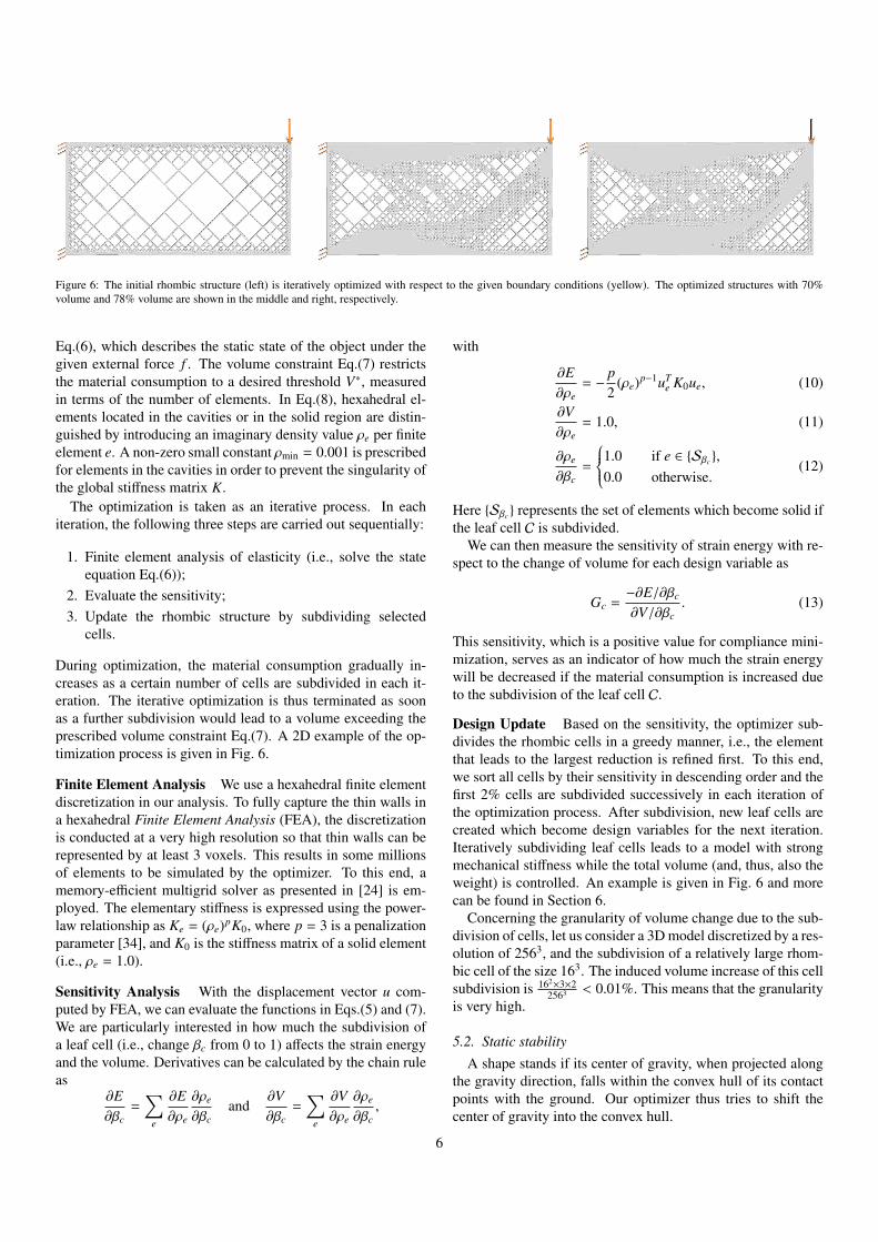
Figure 6: The initial rhombic structure (left) is iteratively optimized with respect to the given boundary conditions (yellow). The optimized structures with 70%volume and 78% volume are shown in the middle and right, respectively.

Eq.(6), which describes the static state of the object under thegiven external force f . The volume constraint Eq.(7) restrictsthe material consumption to a desired threshold V∗, measuredin terms of the number of elements. In Eq.(8), hexahedral el-ements located in the cavities or in the solid region are distin-guished by introducing an imaginary density value ρe per finiteelement e. A non-zero small constant ρmin = 0.001 is prescribedfor elements in the cavities in order to prevent the singularity ofthe global stiffness matrix K.

The optimization is taken as an iterative process. In eachiteration, the following three steps are carried out sequentially:

1. Finite element analysis of elasticity (i.e., solve the stateequation Eq.(6));

2. Evaluate the sensitivity;3. Update the rhombic structure by subdividing selected

cells.

During optimization, the material consumption gradually in-creases as a certain number of cells are subdivided in each it-eration. The iterative optimization is thus terminated as soonas a further subdivision would lead to a volume exceeding theprescribed volume constraint Eq.(7). A 2D example of the op-timization process is given in Fig. 6.

Finite Element Analysis We use a hexahedral finite elementdiscretization in our analysis. To fully capture the thin walls ina hexahedral Finite Element Analysis (FEA), the discretizationis conducted at a very high resolution so that thin walls can berepresented by at least 3 voxels. This results in some millionsof elements to be simulated by the optimizer. To this end, amemory-efficient multigrid solver as presented in [24] is em-ployed. The elementary stiffness is expressed using the power-law relationship as Ke = (ρe)pK0, where p = 3 is a penalizationparameter [34], and K0 is the stiffness matrix of a solid element(i.e., ρe = 1.0).

Sensitivity Analysis With the displacement vector u com-puted by FEA, we can evaluate the functions in Eqs.(5) and (7).We are particularly interested in how much the subdivision ofa leaf cell (i.e., change βc from 0 to 1) affects the strain energyand the volume. Derivatives can be calculated by the chain ruleas

∂E∂βc

=∑

e

∂E∂ρe

∂ρe

∂βcand

∂V∂βc

=∑

e

∂V∂ρe

∂ρe

∂βc,

with

∂E∂ρe

= −p2

(ρe)p−1uTe K0ue, (10)

∂V∂ρe

= 1.0, (11)

∂ρe

∂βc=

1.0 if e ∈ Sβc ,0.0 otherwise.

(12)

Here Sβc represents the set of elements which become solid ifthe leaf cell C is subdivided.

We can then measure the sensitivity of strain energy with re-spect to the change of volume for each design variable as

Gc =−∂E/∂βc

∂V/∂βc. (13)

This sensitivity, which is a positive value for compliance mini-mization, serves as an indicator of how much the strain energywill be decreased if the material consumption is increased dueto the subdivision of the leaf cell C.

Design Update Based on the sensitivity, the optimizer sub-divides the rhombic cells in a greedy manner, i.e., the elementthat leads to the largest reduction is refined first. To this end,we sort all cells by their sensitivity in descending order and thefirst 2% cells are subdivided successively in each iteration ofthe optimization process. After subdivision, new leaf cells arecreated which become design variables for the next iteration.Iteratively subdividing leaf cells leads to a model with strongmechanical stiffness while the total volume (and, thus, also theweight) is controlled. An example is given in Fig. 6 and morecan be found in Section 6.

Concerning the granularity of volume change due to the sub-division of cells, let us consider a 3D model discretized by a res-olution of 2563, and the subdivision of a relatively large rhom-bic cell of the size 163. The induced volume increase of this cellsubdivision is 162×3×2

2563 < 0.01%. This means that the granularityis very high.

5.2. Static stability

A shape stands if its center of gravity, when projected alongthe gravity direction, falls within the convex hull of its contactpoints with the ground. Our optimizer thus tries to shift thecenter of gravity into the convex hull.

6

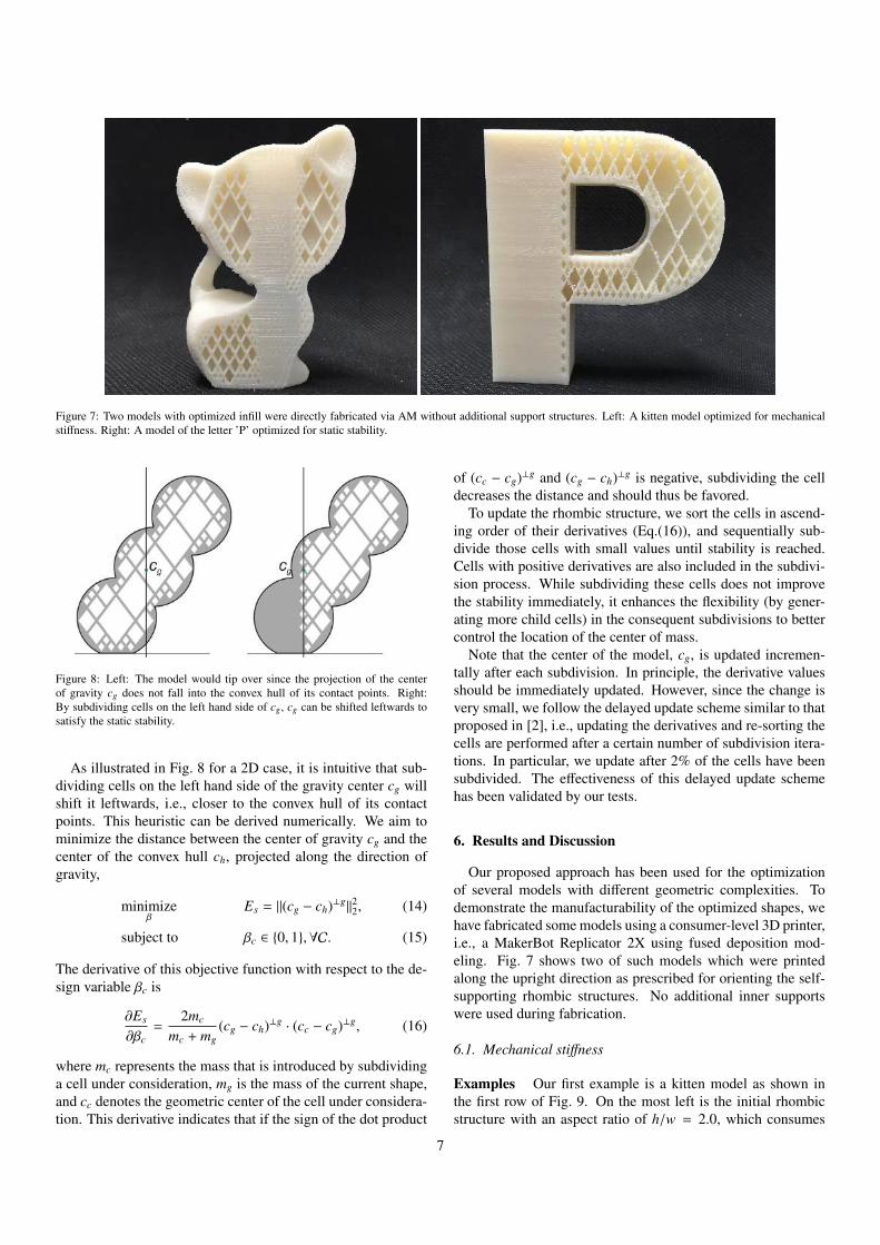
Figure 7: Two models with optimized infill were directly fabricated via AM without additional support structures. Left: A kitten model optimized for mechanicalstiffness. Right: A model of the letter ’P’ optimized for static stability.

Figure 8: Left: The model would tip over since the projection of the centerof gravity cg does not fall into the convex hull of its contact points. Right:By subdividing cells on the left hand side of cg, cg can be shifted leftwards tosatisfy the static stability.

As illustrated in Fig. 8 for a 2D case, it is intuitive that sub-dividing cells on the left hand side of the gravity center cg willshift it leftwards, i.e., closer to the convex hull of its contactpoints. This heuristic can be derived numerically. We aim tominimize the distance between the center of gravity cg and thecenter of the convex hull ch, projected along the direction ofgravity,

minimizeβ

Es = ‖(cg − ch)⊥g‖22, (14)

subject to βc ∈ 0, 1,∀C. (15)

The derivative of this objective function with respect to the de-sign variable βc is

∂Es

∂βc=

2mc

mc + mg(cg − ch)⊥g · (cc − cg)⊥g, (16)

where mc represents the mass that is introduced by subdividinga cell under consideration, mg is the mass of the current shape,and cc denotes the geometric center of the cell under considera-tion. This derivative indicates that if the sign of the dot product

of (cc − cg)⊥g and (cg − ch)⊥g is negative, subdividing the celldecreases the distance and should thus be favored.

To update the rhombic structure, we sort the cells in ascend-ing order of their derivatives (Eq.(16)), and sequentially sub-divide those cells with small values until stability is reached.Cells with positive derivatives are also included in the subdivi-sion process. While subdividing these cells does not improvethe stability immediately, it enhances the flexibility (by gener-ating more child cells) in the consequent subdivisions to bettercontrol the location of the center of mass.

Note that the center of the model, cg, is updated incremen-tally after each subdivision. In principle, the derivative valuesshould be immediately updated. However, since the change isvery small, we follow the delayed update scheme similar to thatproposed in [2], i.e., updating the derivatives and re-sorting thecells are performed after a certain number of subdivision itera-tions. In particular, we update after 2% of the cells have beensubdivided. The effectiveness of this delayed update schemehas been validated by our tests.

6. Results and Discussion

Our proposed approach has been used for the optimizationof several models with different geometric complexities. Todemonstrate the manufacturability of the optimized shapes, wehave fabricated some models using a consumer-level 3D printer,i.e., a MakerBot Replicator 2X using fused deposition mod-eling. Fig. 7 shows two of such models which were printedalong the upright direction as prescribed for orienting the self-supporting rhombic structures. No additional inner supportswere used during fabrication.

6.1. Mechanical stiffness

Examples Our first example is a kitten model as shown inthe first row of Fig. 9. On the most left is the initial rhombicstructure with an aspect ratio of h/w = 2.0, which consumes

7

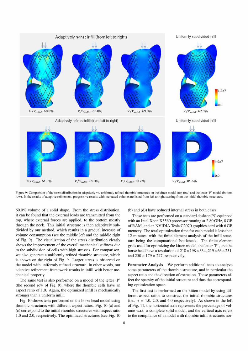
Figure 9: Comparison of the stress distribution in adaptively vs. uniformly refined rhombic structures on the kitten model (top row) and the letter ‘P’ model (bottomrow). In the results of adaptive refinement, progressive results with increased volume are listed from left to right starting from the initial rhombic structures.

60.0% volume of a solid shape. From the stress distribution,it can be found that the external loads are transmitted from thetop, where external forces are applied, to the bottom mostlythrough the neck. This initial structure is then adaptively sub-divided by our method, which results in a gradual increase ofvolume consumption (see the middle left and the middle rightof Fig. 9). The visualization of the stress distribution clearlyshows the improvement of the overall mechanical stiffness dueto the subdivision of cells with high stresses. For comparison,we also generate a uniformly refined rhombic structure, whichis shown on the right of Fig. 9. Larger stress is observed onthe model with uniformly refined structure. In other words, ouradaptive refinement framework results in infill with better me-chanical property.

The same test is also performed on a model of the letter ‘P’(the second row of Fig. 9), where the rhombic cells have anaspect ratio of 1.0. Again, the optimized infill is mechanicallystronger than a uniform infill.

Fig. 10 shows tests performed on the horse head model usingrhombic structures with different aspect ratios. Fig. 10 (a) and(c) correspond to the initial rhombic structures with aspect ratio1.0 and 2.0, respectively. The optimized structures (see Fig. 10

(b) and (d)) have reduced internal stress in both cases.These tests are performed on a standard desktop PC equipped

with an Intel Xeon X5560 processor running at 2.80 GHz, 8 GBof RAM, and an NVIDIA Tesla C2070 graphics card with 6 GBmemory. The total optimization time for each model is less than12 minutes, with the finite element analysis of the infill struc-ture being the computational bottleneck. The finite elementgrids used for optimizing the kitten model, the letter ’P’, and thehorse head have a resolution of 218×198×334, 219×63×251,and 250 × 179 × 247, respectively.

Parameter Analysis We perform additional tests to analyzesome parameters of the rhombic structure, and in particular theaspect ratio and the direction of extrusion. These parameters af-fect the sparsity of the initial structure and thus the correspond-ing optimization space.

The first test is performed on the kitten model by using dif-ferent aspect ratios to construct the initial rhombic structures(i.e., α = 1.0, 2.0, and 4.0 respectively). As shown in the leftof Fig. 11, the horizontal axis represents the percentage of vol-ume w.r.t. a complete solid model, and the vertical axis refersto the compliance of a model with rhombic infill structures nor-

8

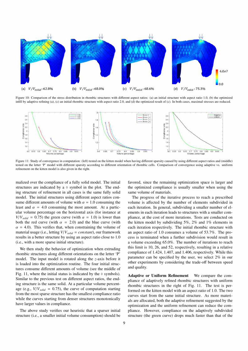
Figure 10: Comparison of the stress distribution in rhombic structures with different aspect ratios: (a) an initial structure with aspect ratio 1.0, (b) the optimizedinfill by adaptive refining (a), (c) an initial rhombic structure with aspect ratio 2.0, and (d) the optimized result of (c). In both cases, maximal stresses are reduced.

Figure 11: Study of convergence in computation: (left) tested on the kitten model when having different sparsity caused by using different aspect ratios and (middle)tested on the letter ‘P’ model with different sparsity according to different orientation of rhombic cells. Comparison of convergence using adaptive vs. uniformrefinement on the kitten model is also given in the right.

malized over the compliance of a fully solid model. The initialstructures are indicated by a ♦ symbol in the plot. The end-ing structure of refinement in all cases is the same fully solidmodel. The initial structures using different aspect ratios con-sume different amounts of volume with α = 1.0 consuming theleast and α = 4.0 consuming the most amount. At a partic-ular volume percentage on the horizontal axis (for instance atV/Vsolid = 0.75) the green curve (with α = 1.0) is lower thanboth the red curve (with α = 2.0) and the blue curve (withα = 4.0). This verifies that, when constraining the volume ofmaterial usage (i.e., letting V/Vsolid = constant), our frameworkresults in a better structure by using an aspect ratio close to 1.0(i.e., with a more sparse initial structure).

We then study the behavior of optimization when extrudingrhombic structures along different orientations on the letter ‘P’model. The input model is rotated along the z-axis before itis loaded into the optimization routine. The four initial struc-tures consume different amounts of volume (see the middle ofFig. 11, where the initial status is indicated by the ♦ symbols).Similar to the previous test on different aspect ratios, the end-ing structure is the same solid. At a particular volume percent-age (e.g., V/Vsolid = 0.75), the curve of computation startingfrom the most sparse structure has the smallest compliance ratiowhile the curves starting from denser structures monotonicallyhave larger values in compliance.

The above study verifies our heuristic that a sparser initialstructure (i.e., a smaller initial volume consumption) should be

favored, since the remaining optimization space is larger andthe optimized compliance is usually smaller when using thesame volume of materials.

The progress of the iterative process to reach a prescribedvolume is affected by the number of elements subdivided ineach iteration. In general, subdividing a smaller number of el-ements in each iteration leads to structures with a smaller com-pliance, at the cost of more iterations. Tests are conducted onthe kitten model by subdividing 5%, 2% and 1% elements ineach iteration respectively. The initial rhombic structure withan aspect ratio of 1.0 consumes a volume of 53.7%. The pro-cess is terminated when a further subdivision would result ina volume exceeding 65.0%. The number of iterations to reachthis limit is 10, 26, and 52, respectively, resulting in a relativecompliance of 1.424, 1.407, and 1.406, respectively. While thisparameter can be specified by the user, we select 2% in ourother experiments by considering the trade-off between speedand quality.

Adaptive or Uniform Refinement We compare the com-pliance of adaptively refined rhombic structures with uniformrhombic structures in the right of Fig. 11. The test is per-formed on the kitten model with an aspect ratio of 1.0. The twocurves start from the same initial structure. As more materi-als are allocated, both the adaptive refinement suggested by theoptimization and the uniform refinement can reduce the com-pliance. However, compliance on the adaptively subdividedstructure (the green curve) drops much faster than that of the

9

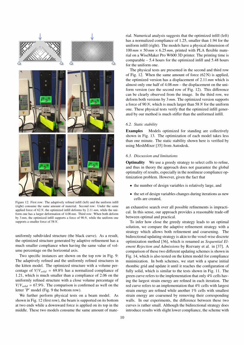
Figure 12: First row: The adaptively refined infill (left) and the uniform infill(right) consume the same amount of material. Second row: Under the sameapplied force of 62 N, the optimized infill deforms by 2.11 mm, while the uni-form one has a larger deformation of 4.08 mm. Third row: When both deformby 3 mm, the optimized infill supports a force of 90 N, while the uniform onesupports a smaller force of 58 N.

uniformly subdivided structure (the black curve). As a result,the optimized structure generated by adaptive refinement has amuch smaller compliance when having the same value of vol-ume percentage on the horizontal axis.

Two specific instances are shown on the top row in Fig. 9:The adaptively refined and the uniformly refined structures inthe kitten model. The optimized structure with a volume per-centage of V/Vsolid = 69.8% has a normalized compliance of1.21, which is much smaller than a compliance of 2.06 on theuniformly refined structure with a close volume percentage ofV/Vsolid = 67.9%. The comparison is confirmed as well on theletter ’P’ model (Fig. 9 the bottom row).

We further perform physical tests on a beam model. Asshown in Fig. 12 (first row), the beam is supported on its bottomat two ends while a downward force is applied on its top in themiddle. These two models consume the same amount of mate-

rial. Numerical analysis suggests that the optimized infill (left)has a normalized compliance of 1.25, smaller than 1.94 for theuniform infill (right). The models have a physical dimension of100 mm × 50 mm × 6.25 mm, printed with PLA flexible mate-rial on a WiseMaker Pro W600 3D printer. The printing time iscomparable – 5.4 hours for the optimized infill and 5.48 hoursfor the uniform one.

The physical tests are presented in the second and third rowof Fig. 12. When the same amount of force (62 N) is applied,the optimized version has a displacement of 2.11 mm which isalmost only one half of 4.08 mm – the displacement on the uni-form version (see the second row of Fig. 12). This differencecan be clearly observed from the image. In the third row, wedeform both versions by 3 mm. The optimized version supportsa force of 90 N, which is much larger than 58 N for the uniformone. These physical tests verify that the optimized infill gener-ated by our method is much stiffer than the uniformed infill.

6.2. Static stability

Examples Models optimized for standing are collectivelyshown in Fig. 13. The optimization of each model takes lessthan one minute. The static stability shown here is verified byusing MeshMixer [35] from Autodesk.

6.3. Discussion and limitations

Optimality We use a greedy strategy to select cells to refine,and thus in theory the approach does not guarantee the globaloptimality of results, especially in the nonlinear compliance op-timization problem. However, given the fact that

• the number of design variables is relatively large, and

• the set of design variables changes during iterations as newcells are created,

an exhaustive search over all possible refinements is impracti-cal. In this sense, our approach provides a reasonable trade-off

between optimal and practical.To infer how close the greedy strategy leads to an optimal

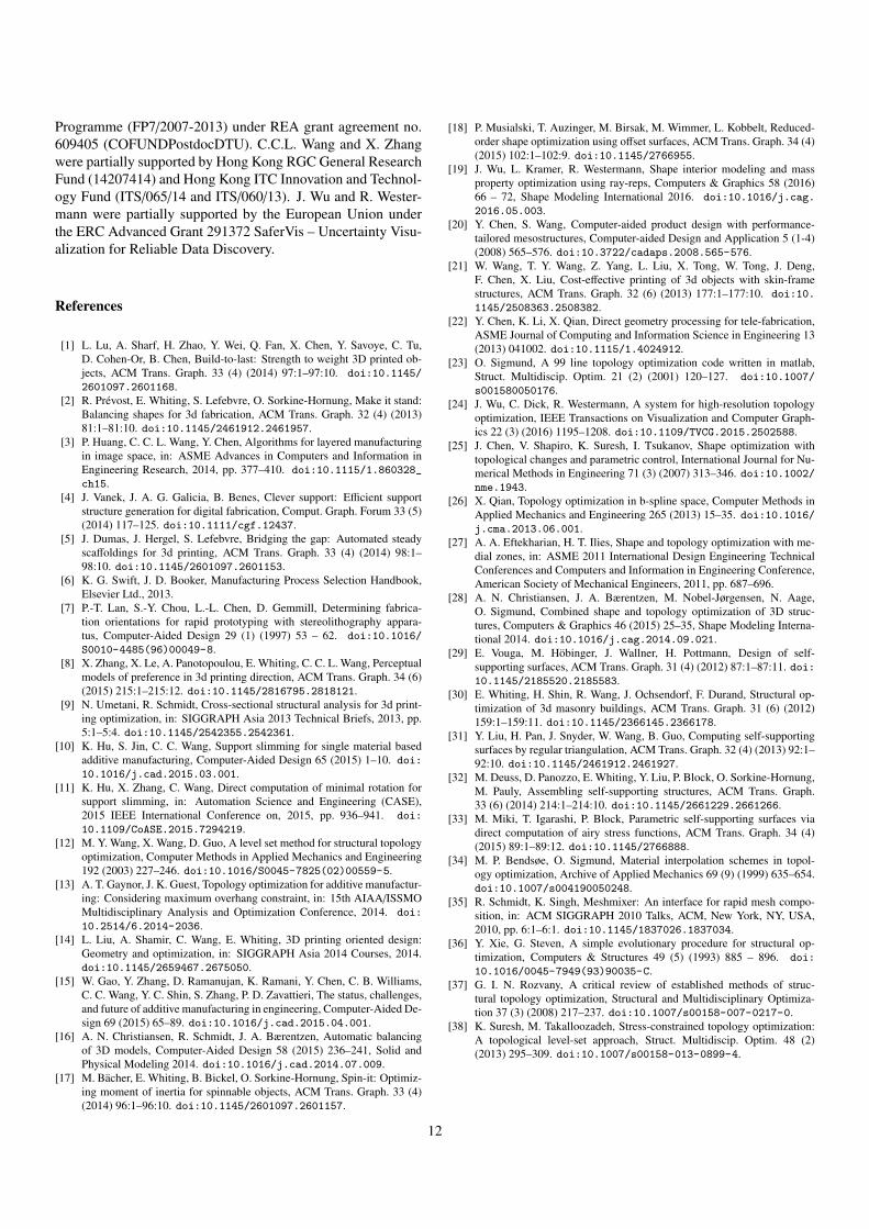
solution, we compare the adaptive refinement strategy with astrategy which allows both refinement and coarsening. Thebidirectional updating strategy is akin to the voxel-wise discreteoptimization method [36], which is renamed as Sequential El-ement Rejection and Admissions by Rozvany et al. in [37]. Acomparison of these two different updating schemes is shown inFig. 14, which is also tested on the kitten model for complianceminimization. In both schemes, we start with a sparse initialrhombic grid and update it until it reaches the configuration offully solid, which is similar to the tests shown in Fig. 11. Thegreen curve refers to the implementation that only 4% cells hav-ing the largest strain energy are refined in each iteration. Thered curve refers to an implementation that 4% cells with largeststrain energy are refined while another 1% cells with smalleststrain energy are coarsened by removing their correspondingwalls. In our experiments, the difference between these twocurves is rather small. Although the bidirectional strategy doesintroduce results with slight lower compliance, the scheme with

10

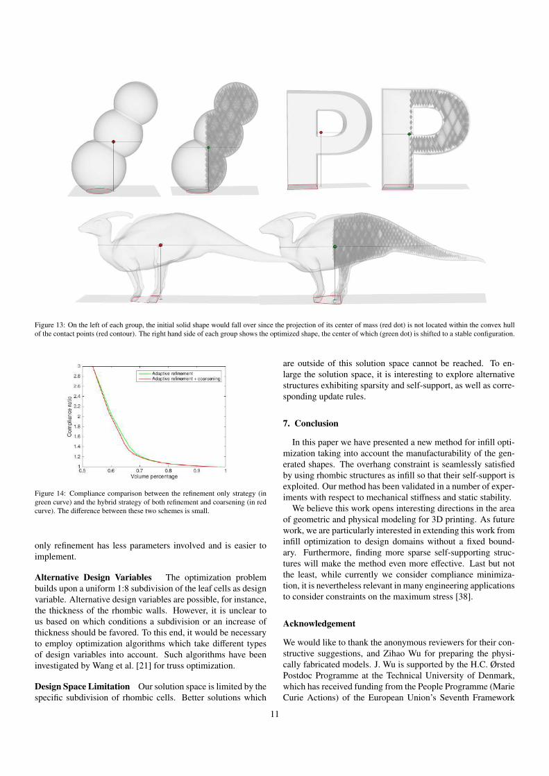
Figure 13: On the left of each group, the initial solid shape would fall over since the projection of its center of mass (red dot) is not located within the convex hullof the contact points (red contour). The right hand side of each group shows the optimized shape, the center of which (green dot) is shifted to a stable configuration.

Figure 14: Compliance comparison between the refinement only strategy (ingreen curve) and the hybrid strategy of both refinement and coarsening (in redcurve). The difference between these two schemes is small.

only refinement has less parameters involved and is easier toimplement.

Alternative Design Variables The optimization problembuilds upon a uniform 1:8 subdivision of the leaf cells as designvariable. Alternative design variables are possible, for instance,the thickness of the rhombic walls. However, it is unclear tous based on which conditions a subdivision or an increase ofthickness should be favored. To this end, it would be necessaryto employ optimization algorithms which take different typesof design variables into account. Such algorithms have beeninvestigated by Wang et al. [21] for truss optimization.

Design Space Limitation Our solution space is limited by thespecific subdivision of rhombic cells. Better solutions which

are outside of this solution space cannot be reached. To en-large the solution space, it is interesting to explore alternativestructures exhibiting sparsity and self-support, as well as corre-sponding update rules.

7. Conclusion

In this paper we have presented a new method for infill opti-mization taking into account the manufacturability of the gen-erated shapes. The overhang constraint is seamlessly satisfiedby using rhombic structures as infill so that their self-support isexploited. Our method has been validated in a number of exper-iments with respect to mechanical stiffness and static stability.

We believe this work opens interesting directions in the areaof geometric and physical modeling for 3D printing. As futurework, we are particularly interested in extending this work frominfill optimization to design domains without a fixed bound-ary. Furthermore, finding more sparse self-supporting struc-tures will make the method even more effective. Last but notthe least, while currently we consider compliance minimiza-tion, it is nevertheless relevant in many engineering applicationsto consider constraints on the maximum stress [38].

Acknowledgement

We would like to thank the anonymous reviewers for their con-structive suggestions, and Zihao Wu for preparing the physi-cally fabricated models. J. Wu is supported by the H.C. ØrstedPostdoc Programme at the Technical University of Denmark,which has received funding from the People Programme (MarieCurie Actions) of the European Union’s Seventh Framework

11

Programme (FP7/2007-2013) under REA grant agreement no.609405 (COFUNDPostdocDTU). C.C.L. Wang and X. Zhangwere partially supported by Hong Kong RGC General ResearchFund (14207414) and Hong Kong ITC Innovation and Technol-ogy Fund (ITS/065/14 and ITS/060/13). J. Wu and R. Wester-mann were partially supported by the European Union underthe ERC Advanced Grant 291372 SaferVis – Uncertainty Visu-alization for Reliable Data Discovery.

References

[1] L. Lu, A. Sharf, H. Zhao, Y. Wei, Q. Fan, X. Chen, Y. Savoye, C. Tu,D. Cohen-Or, B. Chen, Build-to-last: Strength to weight 3D printed ob-jects, ACM Trans. Graph. 33 (4) (2014) 97:1–97:10. doi:10.1145/

2601097.2601168.[2] R. Prevost, E. Whiting, S. Lefebvre, O. Sorkine-Hornung, Make it stand:

Balancing shapes for 3d fabrication, ACM Trans. Graph. 32 (4) (2013)81:1–81:10. doi:10.1145/2461912.2461957.

[3] P. Huang, C. C. L. Wang, Y. Chen, Algorithms for layered manufacturingin image space, in: ASME Advances in Computers and Information inEngineering Research, 2014, pp. 377–410. doi:10.1115/1.860328_

ch15.[4] J. Vanek, J. A. G. Galicia, B. Benes, Clever support: Efficient support

structure generation for digital fabrication, Comput. Graph. Forum 33 (5)(2014) 117–125. doi:10.1111/cgf.12437.

[5] J. Dumas, J. Hergel, S. Lefebvre, Bridging the gap: Automated steadyscaffoldings for 3d printing, ACM Trans. Graph. 33 (4) (2014) 98:1–98:10. doi:10.1145/2601097.2601153.

[6] K. G. Swift, J. D. Booker, Manufacturing Process Selection Handbook,Elsevier Ltd., 2013.

[7] P.-T. Lan, S.-Y. Chou, L.-L. Chen, D. Gemmill, Determining fabrica-tion orientations for rapid prototyping with stereolithography appara-tus, Computer-Aided Design 29 (1) (1997) 53 – 62. doi:10.1016/

S0010-4485(96)00049-8.[8] X. Zhang, X. Le, A. Panotopoulou, E. Whiting, C. C. L. Wang, Perceptual

models of preference in 3d printing direction, ACM Trans. Graph. 34 (6)(2015) 215:1–215:12. doi:10.1145/2816795.2818121.

[9] N. Umetani, R. Schmidt, Cross-sectional structural analysis for 3d print-ing optimization, in: SIGGRAPH Asia 2013 Technical Briefs, 2013, pp.5:1–5:4. doi:10.1145/2542355.2542361.

[10] K. Hu, S. Jin, C. C. Wang, Support slimming for single material basedadditive manufacturing, Computer-Aided Design 65 (2015) 1–10. doi:

10.1016/j.cad.2015.03.001.[11] K. Hu, X. Zhang, C. Wang, Direct computation of minimal rotation for

support slimming, in: Automation Science and Engineering (CASE),2015 IEEE International Conference on, 2015, pp. 936–941. doi:

10.1109/CoASE.2015.7294219.[12] M. Y. Wang, X. Wang, D. Guo, A level set method for structural topology

optimization, Computer Methods in Applied Mechanics and Engineering192 (2003) 227–246. doi:10.1016/S0045-7825(02)00559-5.

[13] A. T. Gaynor, J. K. Guest, Topology optimization for additive manufactur-ing: Considering maximum overhang constraint, in: 15th AIAA/ISSMOMultidisciplinary Analysis and Optimization Conference, 2014. doi:

10.2514/6.2014-2036.[14] L. Liu, A. Shamir, C. Wang, E. Whiting, 3D printing oriented design:

Geometry and optimization, in: SIGGRAPH Asia 2014 Courses, 2014.doi:10.1145/2659467.2675050.

[15] W. Gao, Y. Zhang, D. Ramanujan, K. Ramani, Y. Chen, C. B. Williams,C. C. Wang, Y. C. Shin, S. Zhang, P. D. Zavattieri, The status, challenges,and future of additive manufacturing in engineering, Computer-Aided De-sign 69 (2015) 65–89. doi:10.1016/j.cad.2015.04.001.

[16] A. N. Christiansen, R. Schmidt, J. A. Bærentzen, Automatic balancingof 3D models, Computer-Aided Design 58 (2015) 236–241, Solid andPhysical Modeling 2014. doi:10.1016/j.cad.2014.07.009.

[17] M. Bacher, E. Whiting, B. Bickel, O. Sorkine-Hornung, Spin-it: Optimiz-ing moment of inertia for spinnable objects, ACM Trans. Graph. 33 (4)(2014) 96:1–96:10. doi:10.1145/2601097.2601157.

[18] P. Musialski, T. Auzinger, M. Birsak, M. Wimmer, L. Kobbelt, Reduced-order shape optimization using offset surfaces, ACM Trans. Graph. 34 (4)(2015) 102:1–102:9. doi:10.1145/2766955.

[19] J. Wu, L. Kramer, R. Westermann, Shape interior modeling and massproperty optimization using ray-reps, Computers & Graphics 58 (2016)66 – 72, Shape Modeling International 2016. doi:10.1016/j.cag.

2016.05.003.[20] Y. Chen, S. Wang, Computer-aided product design with performance-

tailored mesostructures, Computer-aided Design and Application 5 (1-4)(2008) 565–576. doi:10.3722/cadaps.2008.565-576.

[21] W. Wang, T. Y. Wang, Z. Yang, L. Liu, X. Tong, W. Tong, J. Deng,F. Chen, X. Liu, Cost-effective printing of 3d objects with skin-framestructures, ACM Trans. Graph. 32 (6) (2013) 177:1–177:10. doi:10.

1145/2508363.2508382.[22] Y. Chen, K. Li, X. Qian, Direct geometry processing for tele-fabrication,

ASME Journal of Computing and Information Science in Engineering 13(2013) 041002. doi:10.1115/1.4024912.

[23] O. Sigmund, A 99 line topology optimization code written in matlab,Struct. Multidiscip. Optim. 21 (2) (2001) 120–127. doi:10.1007/

s001580050176.[24] J. Wu, C. Dick, R. Westermann, A system for high-resolution topology

optimization, IEEE Transactions on Visualization and Computer Graph-ics 22 (3) (2016) 1195–1208. doi:10.1109/TVCG.2015.2502588.

[25] J. Chen, V. Shapiro, K. Suresh, I. Tsukanov, Shape optimization withtopological changes and parametric control, International Journal for Nu-merical Methods in Engineering 71 (3) (2007) 313–346. doi:10.1002/nme.1943.

[26] X. Qian, Topology optimization in b-spline space, Computer Methods inApplied Mechanics and Engineering 265 (2013) 15–35. doi:10.1016/j.cma.2013.06.001.

[27] A. A. Eftekharian, H. T. Ilies, Shape and topology optimization with me-dial zones, in: ASME 2011 International Design Engineering TechnicalConferences and Computers and Information in Engineering Conference,American Society of Mechanical Engineers, 2011, pp. 687–696.

[28] A. N. Christiansen, J. A. Bærentzen, M. Nobel-Jørgensen, N. Aage,O. Sigmund, Combined shape and topology optimization of 3D struc-tures, Computers & Graphics 46 (2015) 25–35, Shape Modeling Interna-tional 2014. doi:10.1016/j.cag.2014.09.021.

[29] E. Vouga, M. Hobinger, J. Wallner, H. Pottmann, Design of self-supporting surfaces, ACM Trans. Graph. 31 (4) (2012) 87:1–87:11. doi:10.1145/2185520.2185583.

[30] E. Whiting, H. Shin, R. Wang, J. Ochsendorf, F. Durand, Structural op-timization of 3d masonry buildings, ACM Trans. Graph. 31 (6) (2012)159:1–159:11. doi:10.1145/2366145.2366178.

[31] Y. Liu, H. Pan, J. Snyder, W. Wang, B. Guo, Computing self-supportingsurfaces by regular triangulation, ACM Trans. Graph. 32 (4) (2013) 92:1–92:10. doi:10.1145/2461912.2461927.

[32] M. Deuss, D. Panozzo, E. Whiting, Y. Liu, P. Block, O. Sorkine-Hornung,M. Pauly, Assembling self-supporting structures, ACM Trans. Graph.33 (6) (2014) 214:1–214:10. doi:10.1145/2661229.2661266.

[33] M. Miki, T. Igarashi, P. Block, Parametric self-supporting surfaces viadirect computation of airy stress functions, ACM Trans. Graph. 34 (4)(2015) 89:1–89:12. doi:10.1145/2766888.

[34] M. P. Bendsøe, O. Sigmund, Material interpolation schemes in topol-ogy optimization, Archive of Applied Mechanics 69 (9) (1999) 635–654.doi:10.1007/s004190050248.

[35] R. Schmidt, K. Singh, Meshmixer: An interface for rapid mesh compo-sition, in: ACM SIGGRAPH 2010 Talks, ACM, New York, NY, USA,2010, pp. 6:1–6:1. doi:10.1145/1837026.1837034.

[36] Y. Xie, G. Steven, A simple evolutionary procedure for structural op-timization, Computers & Structures 49 (5) (1993) 885 – 896. doi:

10.1016/0045-7949(93)90035-C.[37] G. I. N. Rozvany, A critical review of established methods of struc-

tural topology optimization, Structural and Multidisciplinary Optimiza-tion 37 (3) (2008) 217–237. doi:10.1007/s00158-007-0217-0.

[38] K. Suresh, M. Takalloozadeh, Stress-constrained topology optimization:A topological level-set approach, Struct. Multidiscip. Optim. 48 (2)(2013) 295–309. doi:10.1007/s00158-013-0899-4.

12