1  

SEM- EDS Instruction Manual

Double-click on the Spirit icon ( ) on the desktop to start the software program.

I. X-ray Functions

Access the basic X-ray acquisition, display and analysis functions through either the Xray menus or the X-ray toolbars:

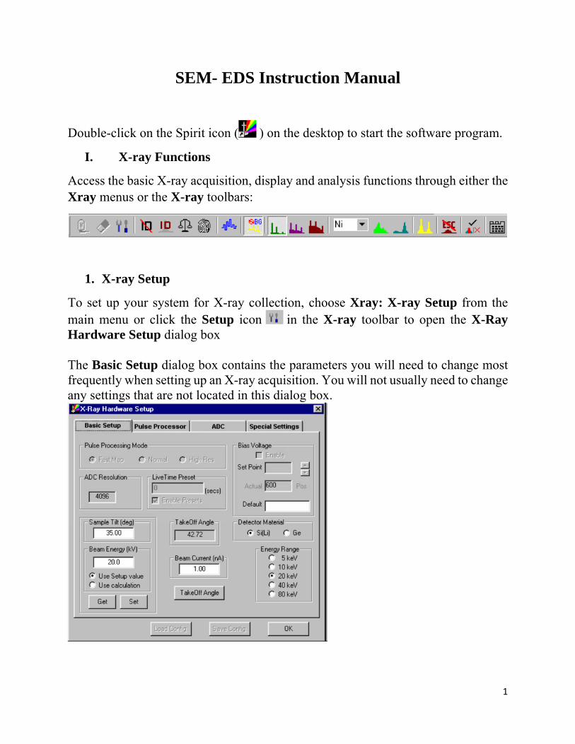
1. X-ray Setup

To set up your system for X-ray collection, choose Xray: X-ray Setup from the main menu or click the Setup icon in the X-ray toolbar to open the X-Ray Hardware Setup dialog box The Basic Setup dialog box contains the parameters you will need to change most frequently when setting up an X-ray acquisition. You will not usually need to change any settings that are not located in this dialog box.

2  

The Pulse Processing Mode panel contains the three commands you will need to change most often:

Fast Map is used to get the greatest possible throughput with some loss of resolution at a

3μs shaping time. Normal provides very good resolution with good throughput at a 12μs

shaping time. High Res (High Resolution) provides the best resolution and low energy

performance, but the lowest throughput at a 24 μs shaping time.

Enter the Live Time Preset (in seconds) in the text box and select Enable Presets. If you enter zero, acquisition will continue until you click Stop.

Type the value directly into the Beam Energy (KV) text box. Click Set to write the entered value to the microscope and apply it to the next spectrum that is collected. Select Use Setup value to apply this value to all collected spectra.

Select the Energy Range you will use for your spectrum

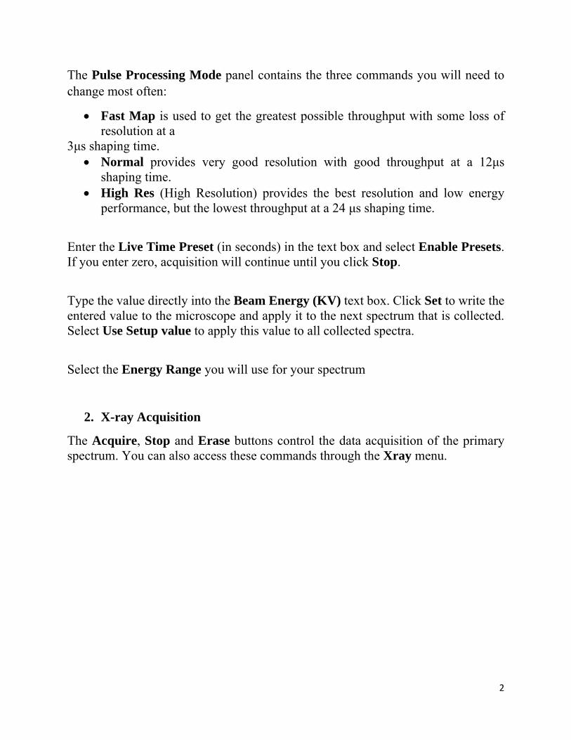
2. X-ray Acquisition

The Acquire, Stop and Erase buttons control the data acquisition of the primary spectrum. You can also access these commands through the Xray menu.

3  

To collect additional spectra, click Acquire again. The existing spectrum display will move to the left and the new displays will open at the right.

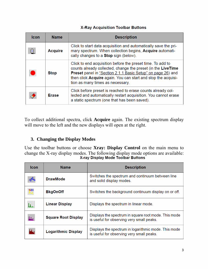
3. Changing the Display Modes

Use the toolbar buttons or choose Xray: Display Control on the main menu to change the X-ray display modes. The following display mode options are available:

4  

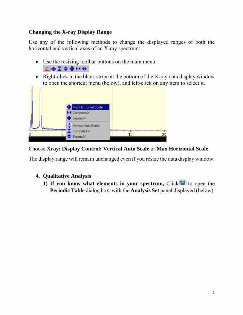
Changing the X-ray Display Range

Use any of the following methods to change the displayed ranges of both the horizontal and vertical axes of an X-ray spectrum:

Use the resizing toolbar buttons on the main menu

Right-click in the black stripe at the bottom of the X-ray data display window

to open the shortcut menu (below), and left-click on any item to select it.

Choose Xray: Display Control: Vertical Auto Scale or Max Horizontal Scale.

The display range will remain unchanged even if you resize the data display window.

4. Qualitative Analysis

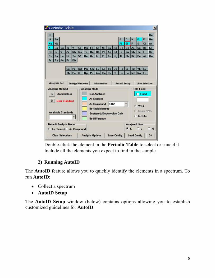
1) If you know what elements in your spectrum, Click to open the Periodic Table dialog box, with the Analysis Set panel displayed (below).

5  

Double-click the element in the Periodic Table to select or cancel it. Include all the elements you expect to find in the sample.

2) Running AutoID

The AutoID feature allows you to quickly identify the elements in a spectrum. To run AutoID:

Collect a spectrum AutoID Setup

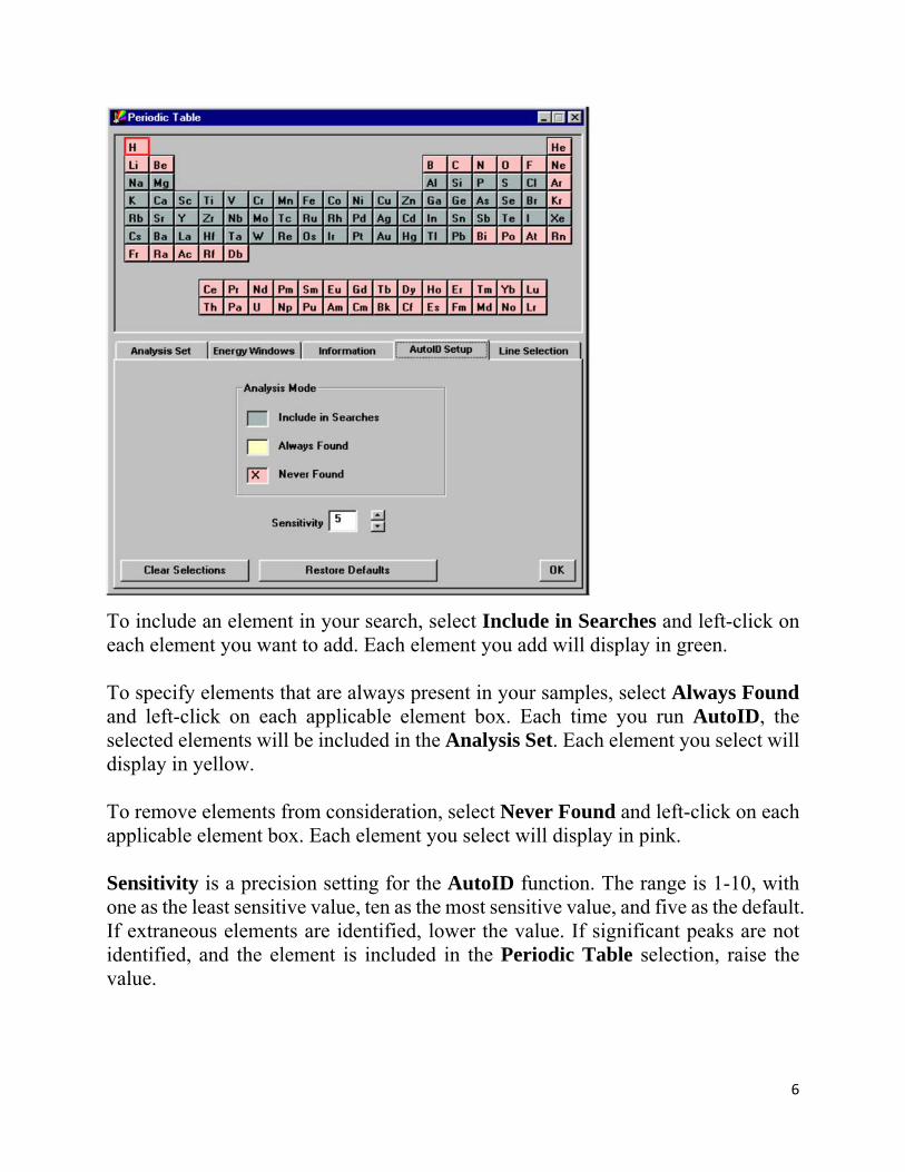
The AutoID Setup window (below) contains options allowing you to establish customized guidelines for AutoID.

6  

To include an element in your search, select Include in Searches and left-click on each element you want to add. Each element you add will display in green. To specify elements that are always present in your samples, select Always Found and left-click on each applicable element box. Each time you run AutoID, the selected elements will be included in the Analysis Set. Each element you select will display in yellow. To remove elements from consideration, select Never Found and left-click on each applicable element box. Each element you select will display in pink. Sensitivity is a precision setting for the AutoID function. The range is 1-10, with one as the least sensitive value, ten as the most sensitive value, and five as the default. If extraneous elements are identified, lower the value. If significant peaks are not identified, and the element is included in the Periodic Table selection, raise the value.

7  

Click Clear Selections to remove all selections. All entries in the Periodic Table will revert to Include in Searches mode. Click Restore Defaults to return to the system default values (shown above). Click OK to save all changes and exit the Periodic Table.

Set Show/Hide KLM Markers to Show ( ).

Set Show/Hide Analysis Labels to Show

Click ( ) to run AutoID.

If AutoID fails to identify significant peaks in your spectrum: • Open the Periodic Table ( ) and click the AutoID Setup tab. • Raise the value of the Sensitivity setting (the maximum value is 10) and click OK. • If the element is at a very low concentration in the sample, only the most intense lines will be detected. To see very weak lines, reduce the peak intensity cutoff. Choose Xray: Preferences and enter the desired setting in the Intensity Cutoff panel.

If AutoID identifies peaks where you don’t think they should be: • Open the Periodic Table ( ) and click the AutoID Setup tab. • Lower the value of the Sensitivity setting (the minimum value is 1) and click OK.

3) If you have already run AutoID on the spectrum, the identified elements are highlighted in cyan. To eliminate a minor or undesired element from the spectrum display, on the Analysis Set panel, select it and choose Not Analyzed. The element will no longer appear as active in the Periodic Table or the spectrum display.

4) Clearing an Analysis Set

Clear Element Set removes all lines and labels corresponding to elements found by AutoID from the spectrum display, and removes the elements from the Periodic Table. 5) Save the spectrum Save the spectrum by clicking on file in the main menu and selecting save. 6) Generate report

Clicking on report in the main menu, selecting spectrum and data to get the report.

8  

5. Quantitative Analysis

1) Selecting an Analysis Type

To select the analysis type: • Open the Periodic Table ( ) and click the Analysis Set tab.

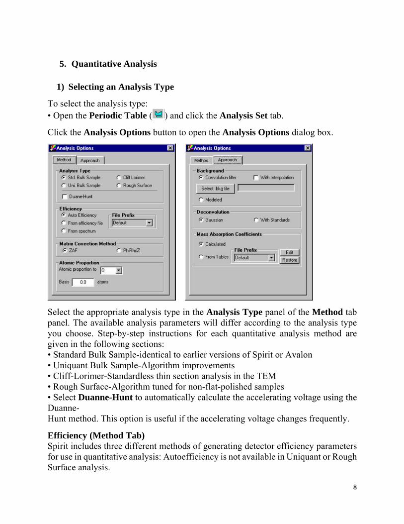
Click the Analysis Options button to open the Analysis Options dialog box.

Select the appropriate analysis type in the Analysis Type panel of the Method tab panel. The available analysis parameters will differ according to the analysis type you choose. Step-by-step instructions for each quantitative analysis method are given in the following sections: • Standard Bulk Sample-identical to earlier versions of Spirit or Avalon • Uniquant Bulk Sample-Algorithm improvements • Cliff-Lorimer-Standardless thin section analysis in the TEM • Rough Surface-Algorithm tuned for non-flat-polished samples • Select Duanne-Hunt to automatically calculate the accelerating voltage using the Duanne- Hunt method. This option is useful if the accelerating voltage changes frequently.

Efficiency (Method Tab) Spirit includes three different methods of generating detector efficiency parameters for use in quantitative analysis: Autoefficiency is not available in Uniquant or Rough Surface analysis.

9  

Auto Efficiency generates reliable efficiency values from the iterative

quantitative analysis process itself, and eliminates the need to create an efficiency file for each different combination of excitation and takeoff angle values. Auto Efficiency is only used with the Standard Bulk analysis.

From efficiency file calculates efficiency values based on a previously created efficiency file saved in the C:\Programs\PGT\Efficiencies directory. See Section 9.17 for instructions on creating efficiency files. Choose the specific file you want to use from the File Prefix list.

From spectrum calculates efficiency values using the efficiency parameters stored in the spectrum header. These parameters are stored in the system at the time of calibration.

Matrix Correction Methods (Method Tab) Spirit offers two matrix correction methods, ZAF and PhiRhoZ.

ZAF is the traditional method of Philibert-Duncumb-Heinrich-Reed. • Z = The atomic number factor. • A = The absorption factor. • F = The fluorescence factor. PhiRhoZ is a newer method using the algorithm of Armstrong. It can give improved results for light elements Atomic Proportion-Calculate quantitative results based on a user-selected number of atoms in a chosen element.

2) Set up Analysis Set

Click to open the Periodic Table dialog box, with the Analysis Set panel displayed (below).

10  

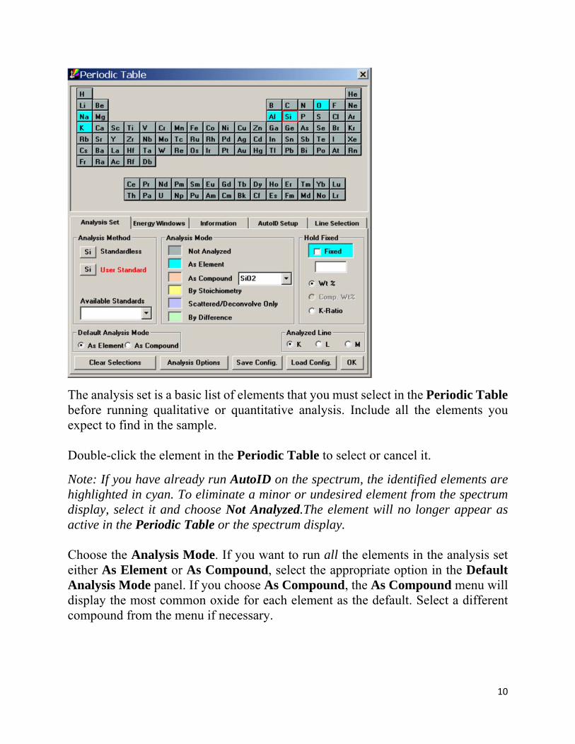
The analysis set is a basic list of elements that you must select in the Periodic Table before running qualitative or quantitative analysis. Include all the elements you expect to find in the sample. Double-click the element in the Periodic Table to select or cancel it.

Note: If you have already run AutoID on the spectrum, the identified elements are highlighted in cyan. To eliminate a minor or undesired element from the spectrum display, select it and choose Not Analyzed.The element will no longer appear as active in the Periodic Table or the spectrum display. Choose the Analysis Mode. If you want to run all the elements in the analysis set either As Element or As Compound, select the appropriate option in the Default Analysis Mode panel. If you choose As Compound, the As Compound menu will display the most common oxide for each element as the default. Select a different compound from the menu if necessary.

11  

Not Analyzed removes an element from the analysis set. You might need to do this if, for example, you previously ran AutoID at a high sensitivity level, and your analysis set contains extraneous elements. • As Element analyzes an element in terms of elemental concentration. • As Compound analyzes an element in terms of elemental concentration, as above. In addition, all elements associated with the primary element through the stoichiometry of the compound will be added to the analysis set, and their concentrations computed by stoichiometry based on the concentration of the primary element. You must choose the compound from the As Compound menu before you select As Compound. Any compound can be added to the list by typing in the chemical formula. • By Stoichiometry calculates concentration by applying the gravimetric factor to each element in the analysis and reporting it as an oxide, sulfide, etc. The stoichiometric element is selected by choosing the correct compound for each element. • Deconvolve Only performs deconvolution on the peak associated with the selected element, but does not consider it for concentration purposes. This function is useful when dealing with artifact due to a coating or stray radiation. • By Difference is available in Uniquant only and is used to define the concentration of one selected element as 100% - the concentration of all the other elements.

If you want to analyze an element without using standards, select No Standards. The system will generate an internal standard based on fundamental parameters calculations. The sum of the concentrations for all elements analyzed using No Standards is normalized to 100%. If you want to run a mixed mode analysis (meaning that some elements are analyzed using standards or held fixed), the elements analyzed using No Standards are normalized to the difference between 100% and the sum of the concentrations of the elements analyzed by standards or held fixed. If you want to analyze an element using standards, you must first select the appropriate standard from the Available Standards menu. This menu contains a list of all the previously created standards contained in the standards database

The Spirit software will automatically select the best K, L or M line for the analysis. You can change this default by selecting a different line in the Analyzed Line panel.

12  

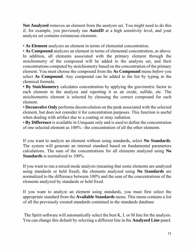
To specify fixed analysis parameters for a material with a known concentration of an element or compound, use Hold Fixed. • Select the element of interest in the Periodic Table. • In the Analysis Mode panel, select either As Element or As Compound. The corresponding commands available for each analysis mode will become active in the Hold Fixed panel.

Select the Fixed check box. If you are analyzing the element As Element: • Select Wt% to fix the weight percent of the element at a specific value. Enter the value into the text box. • Select K-Ratio to fix the K ratio at a specific value. Enter the value, which must be less than one, into the text box. If you are analyzing the element As Compound: • Select Wt% and enter the weight percent of the element into the text box. • Select Comp Wt% and enter the weight percent of the compound into the text box. • Select K-Ratio to fix the K ratio at a specific value. Enter the value, which must be less than one, into the text box.

To undo Hold Fixed, select the element and click Not Analyzed in the Analysis Mode panel.

3) Run the analysis

To run the analysis, click Quantitative Analysis ( ). Spirit immediately generates an analysis report, including data tables, spectra and images, in Microsoft Word.

13  

II. Imaging Functions 1. Image Acquisition Setup

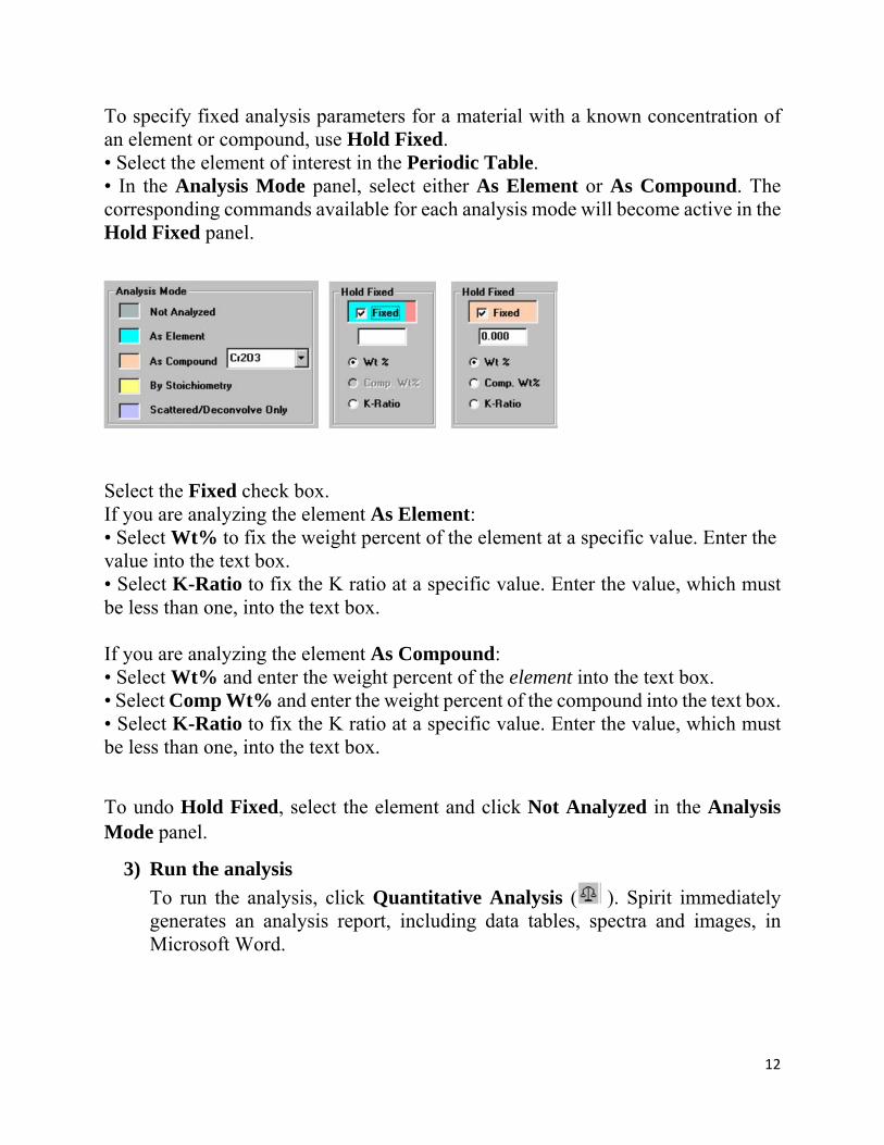
To set up your microscope to collect images, click in the Imaging toolbar or choose Imaging: Setup to open the Image Acquisition Setup dialog box. This dialog box contains two tabs, Preview and Image Sources, that contain commands used to choose and optimize image collection parameters.

1) Click the Preview tab to open the dialog box shown below:

Spirit includes four different image collection Modes: • Rapid collection is the fastest 8-bit image acquisition mode. It can be used only with the two video input channels, which can be set at TV rates (multiple frames/second) if your microscope can support them. Mapping collects an 8-bit image and the associated X-ray information. It can collect data from any input channel. Before collecting maps, run AutoID to determine the

14  

elements present in the sample. Then, manually select the elements you want to map, using the Periodic Table in either the Image Sources. You can map as many elements as you want. High Def. collects an archival quality 16-bit image. It can be used only with the two video input channels, and provides slower scans with more pixel data averaging. Use this mode to collect images used for spotlight analysis and line profile analysis. To collect an image for spotlight analysis, use a scan rate that is slow enough to ensure accurate beam placement on the sample. The actual scan rate depends on the type of microscope you have, and you may need to experiment to determine the correct setting. PTS collects a PTS data cube

The Zoom Mode panel contains four commands: • Full Screen is the normal zoom mode. • Allow Pan & Zoom lets you select and magnify a precise area of your sample.

Zoom lets you choose the Zoom level from the menu (see the instruction in the Using Pan and Zoom section below).

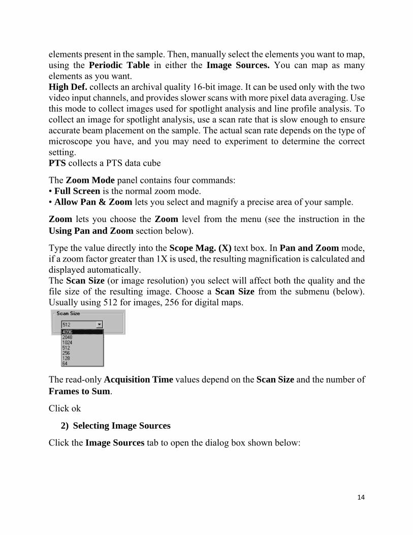
Type the value directly into the Scope Mag. (X) text box. In Pan and Zoom mode, if a zoom factor greater than 1X is used, the resulting magnification is calculated and displayed automatically. The Scan Size (or image resolution) you select will affect both the quality and the file size of the resulting image. Choose a Scan Size from the submenu (below). Usually using 512 for images, 256 for digital maps.

The read-only Acquisition Time values depend on the Scan Size and the number of Frames to Sum.

Click ok

2) Selecting Image Sources

Click the Image Sources tab to open the dialog box shown below:

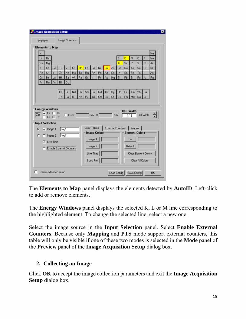
15  

The Elements to Map panel displays the elements detected by AutoID. Left-click to add or remove elements. The Energy Windows panel displays the selected K, L or M line corresponding to the highlighted element. To change the selected line, select a new one. Select the image source in the Input Selection panel. Select Enable External Counters. Because only Mapping and PTS mode support external counters, this table will only be visible if one of these two modes is selected in the Mode panel of the Preview panel of the Image Acquisition Setup dialog box.

2. Collecting an Image

Click OK to accept the image collection parameters and exit the Image Acquisition Setup dialog box.

16  

In the main Spirit display window, choose Imaging: Acquire or click to start image collection.

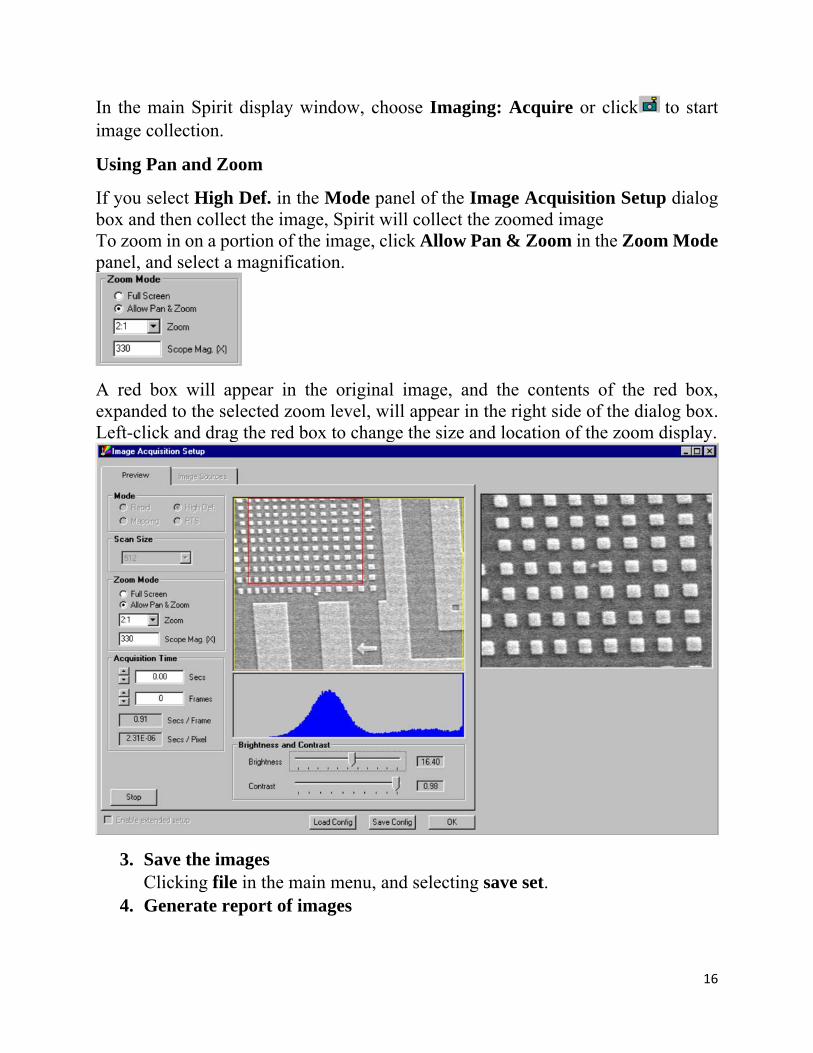
Using Pan and Zoom

If you select High Def. in the Mode panel of the Image Acquisition Setup dialog box and then collect the image, Spirit will collect the zoomed image To zoom in on a portion of the image, click Allow Pan & Zoom in the Zoom Mode panel, and select a magnification.

A red box will appear in the original image, and the contents of the red box, expanded to the selected zoom level, will appear in the right side of the dialog box. Left-click and drag the red box to change the size and location of the zoom display.

3. Save the images Clicking file in the main menu, and selecting save set.

4. Generate report of images

17  

Clicking report in the main menu, and selection set of image to get the report for the whole set of images or selecting image to get the single image report

5. Spotlight Analysis

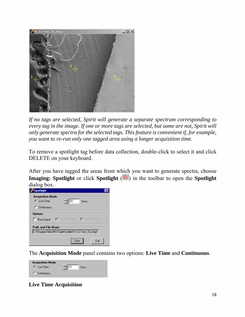
Spotlight analysis allows you to select an unlimited number of specific regions (approximately 5 pixels in diameter) within a live image, and generate a separate spectrum for each consecutively numbered, tagged area. To run spotlight analysis: First, you must collect the image you want to analyze.

Click in the Imaging toolbar or choose Imaging: Setup to open the Image Acquisition Setup dialog box. • In the Mode panel, select High Def. • In the Zoom Mode panel, select Full Screen. • Check the microscope magnification and, if necessary, enter the correct value in the Scope Mag. (X) text box. • Click Preview to start a preview image collection and adjust the contrast and brightness of the image. • Click OK to save the current settings and close the Image Acquisition Setup Dialog box. • In the main Spirit display window, choose Imaging: Acquire or click to start image collection. Next, tag the areas in the image that you want to analyze.

Choose Annotations: Tag. The pointer changes to a crosshair. • Left-click in the image to tag each point at which you want to collect a spectrum. • A numbered spotlight tag marks each tagged area in the image. You can tag an unlimited number of areas in an image.

18  

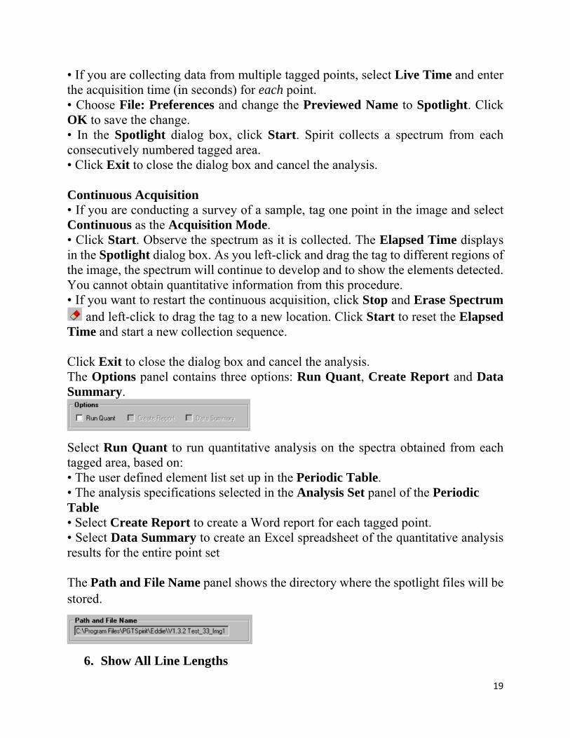
If no tags are selected, Spirit will generate a separate spectrum corresponding to every tag in the image. If one or more tags are selected, but some are not, Spirit will only generate spectra for the selected tags. This feature is convenient if, for example, you want to re-run only one tagged area using a longer acquisition time. To remove a spotlight tag before data collection, double-click to select it and click DELETE on your keyboard. After you have tagged the areas from which you want to generate spectra, choose Imaging: Spotlight or click Spotlight ( ) in the toolbar to open the Spotlight dialog box.

The Acquisition Mode panel contains two options: Live Time and Continuous.

Live Time Acquisition

19  

• If you are collecting data from multiple tagged points, select Live Time and enter the acquisition time (in seconds) for each point. • Choose File: Preferences and change the Previewed Name to Spotlight. Click OK to save the change. • In the Spotlight dialog box, click Start. Spirit collects a spectrum from each consecutively numbered tagged area. • Click Exit to close the dialog box and cancel the analysis. Continuous Acquisition • If you are conducting a survey of a sample, tag one point in the image and select Continuous as the Acquisition Mode. • Click Start. Observe the spectrum as it is collected. The Elapsed Time displays in the Spotlight dialog box. As you left-click and drag the tag to different regions of the image, the spectrum will continue to develop and to show the elements detected. You cannot obtain quantitative information from this procedure. • If you want to restart the continuous acquisition, click Stop and Erase Spectrum

and left-click to drag the tag to a new location. Click Start to reset the Elapsed Time and start a new collection sequence. Click Exit to close the dialog box and cancel the analysis. The Options panel contains three options: Run Quant, Create Report and Data Summary.

Select Run Quant to run quantitative analysis on the spectra obtained from each tagged area, based on: • The user defined element list set up in the Periodic Table. • The analysis specifications selected in the Analysis Set panel of the Periodic Table • Select Create Report to create a Word report for each tagged point. • Select Data Summary to create an Excel spreadsheet of the quantitative analysis results for the entire point set The Path and File Name panel shows the directory where the spotlight files will be stored.

6. Show All Line Lengths

20  

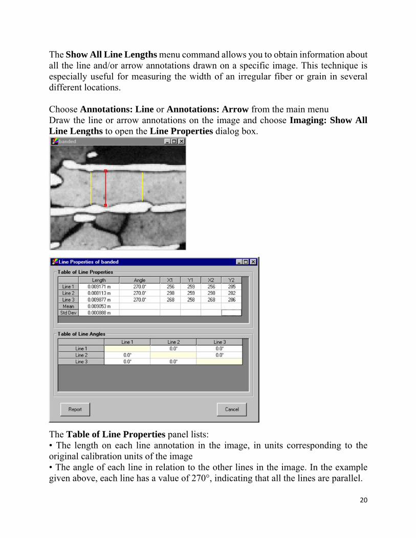
The Show All Line Lengths menu command allows you to obtain information about all the line and/or arrow annotations drawn on a specific image. This technique is especially useful for measuring the width of an irregular fiber or grain in several different locations. Choose Annotations: Line or Annotations: Arrow from the main menu Draw the line or arrow annotations on the image and choose Imaging: Show All Line Lengths to open the Line Properties dialog box.

The Table of Line Properties panel lists: • The length on each line annotation in the image, in units corresponding to the original calibration units of the image • The angle of each line in relation to the other lines in the image. In the example given above, each line has a value of 270°, indicating that all the lines are parallel.

21  

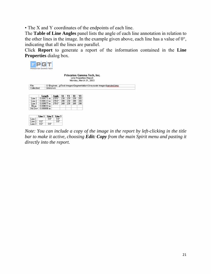
• The X and Y coordinates of the endpoints of each line. The Table of Line Angles panel lists the angle of each line annotation in relation to the other lines in the image. In the example given above, each line has a value of 0°, indicating that all the lines are parallel. Click Report to generate a report of the information contained in the Line Properties dialog box.

Note: You can include a copy of the image in the report by left-clicking in the title bar to make it active, choosing Edit: Copy from the main Spirit menu and pasting it directly into the report.

22  

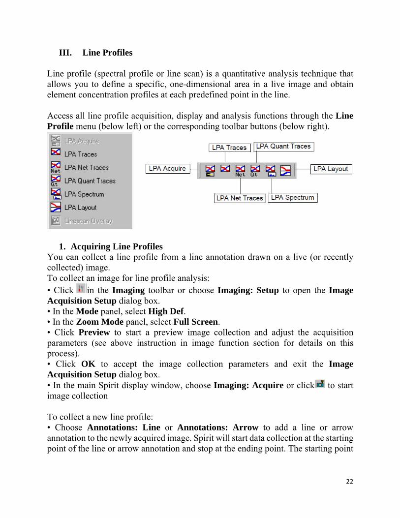
III. Line Profiles

Line profile (spectral profile or line scan) is a quantitative analysis technique that allows you to define a specific, one-dimensional area in a live image and obtain element concentration profiles at each predefined point in the line. Access all line profile acquisition, display and analysis functions through the Line Profile menu (below left) or the corresponding toolbar buttons (below right).

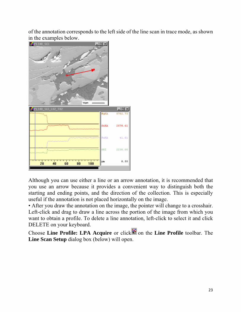
1. Acquiring Line Profiles You can collect a line profile from a line annotation drawn on a live (or recently collected) image. To collect an image for line profile analysis: • Click in the Imaging toolbar or choose Imaging: Setup to open the Image Acquisition Setup dialog box. • In the Mode panel, select High Def. • In the Zoom Mode panel, select Full Screen. • Click Preview to start a preview image collection and adjust the acquisition parameters (see above instruction in image function section for details on this process). • Click OK to accept the image collection parameters and exit the Image Acquisition Setup dialog box. • In the main Spirit display window, choose Imaging: Acquire or click to start image collection To collect a new line profile: • Choose Annotations: Line or Annotations: Arrow to add a line or arrow annotation to the newly acquired image. Spirit will start data collection at the starting point of the line or arrow annotation and stop at the ending point. The starting point

23  

of the annotation corresponds to the left side of the line scan in trace mode, as shown in the examples below.

Although you can use either a line or an arrow annotation, it is recommended that you use an arrow because it provides a convenient way to distinguish both the starting and ending points, and the direction of the collection. This is especially useful if the annotation is not placed horizontally on the image. • After you draw the annotation on the image, the pointer will change to a crosshair. Left-click and drag to draw a line across the portion of the image from which you want to obtain a profile. To delete a line annotation, left-click to select it and click DELETE on your keyboard.

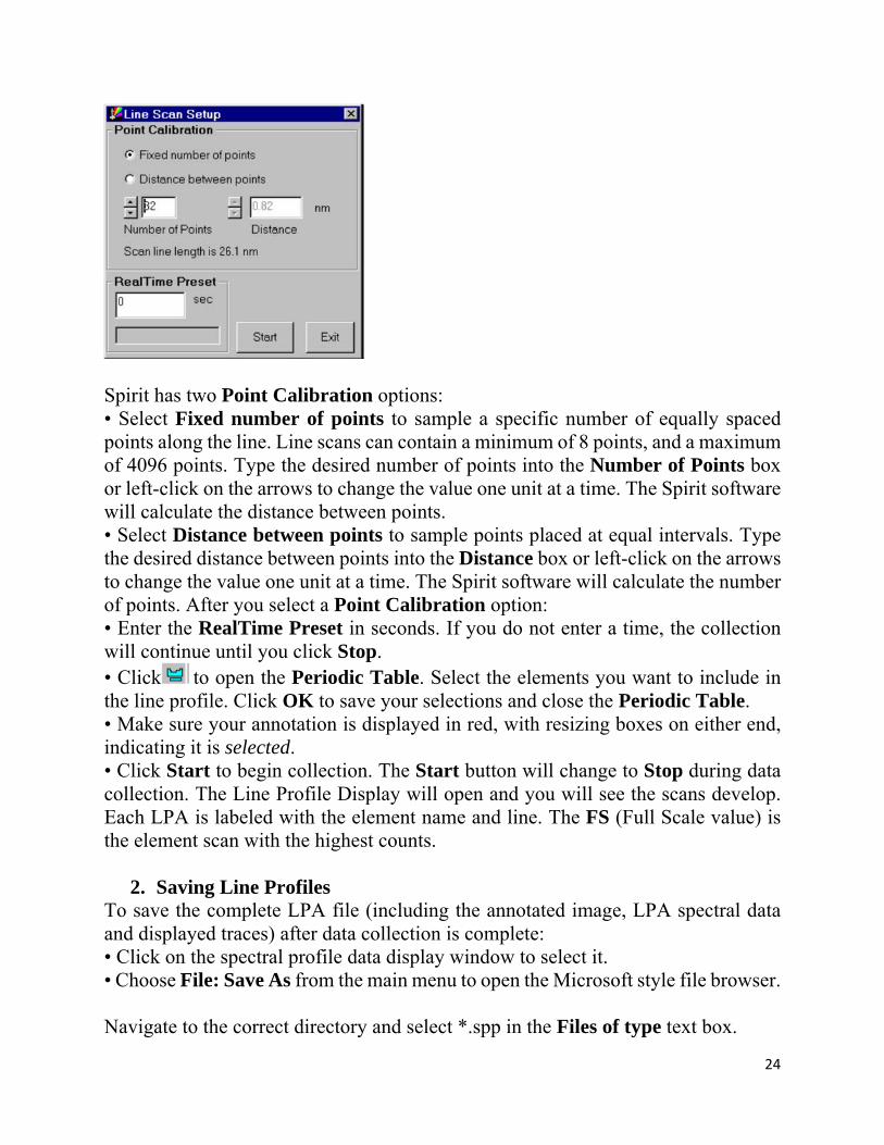
Choose Line Profile: LPA Acquire or click on the Line Profile toolbar. The Line Scan Setup dialog box (below) will open.

24  

Spirit has two Point Calibration options: • Select Fixed number of points to sample a specific number of equally spaced points along the line. Line scans can contain a minimum of 8 points, and a maximum of 4096 points. Type the desired number of points into the Number of Points box or left-click on the arrows to change the value one unit at a time. The Spirit software will calculate the distance between points. • Select Distance between points to sample points placed at equal intervals. Type the desired distance between points into the Distance box or left-click on the arrows to change the value one unit at a time. The Spirit software will calculate the number of points. After you select a Point Calibration option: • Enter the RealTime Preset in seconds. If you do not enter a time, the collection will continue until you click Stop. • Click to open the Periodic Table. Select the elements you want to include in the line profile. Click OK to save your selections and close the Periodic Table. • Make sure your annotation is displayed in red, with resizing boxes on either end, indicating it is selected. • Click Start to begin collection. The Start button will change to Stop during data collection. The Line Profile Display will open and you will see the scans develop. Each LPA is labeled with the element name and line. The FS (Full Scale value) is the element scan with the highest counts.

2. Saving Line Profiles To save the complete LPA file (including the annotated image, LPA spectral data and displayed traces) after data collection is complete: • Click on the spectral profile data display window to select it. • Choose File: Save As from the main menu to open the Microsoft style file browser. Navigate to the correct directory and select *.spp in the Files of type text box.

25  

• In the File Name text box, type a unique name for the file and click Save. You can also save just the traces as an *.lpa file, but this file type does not contain spectral data.

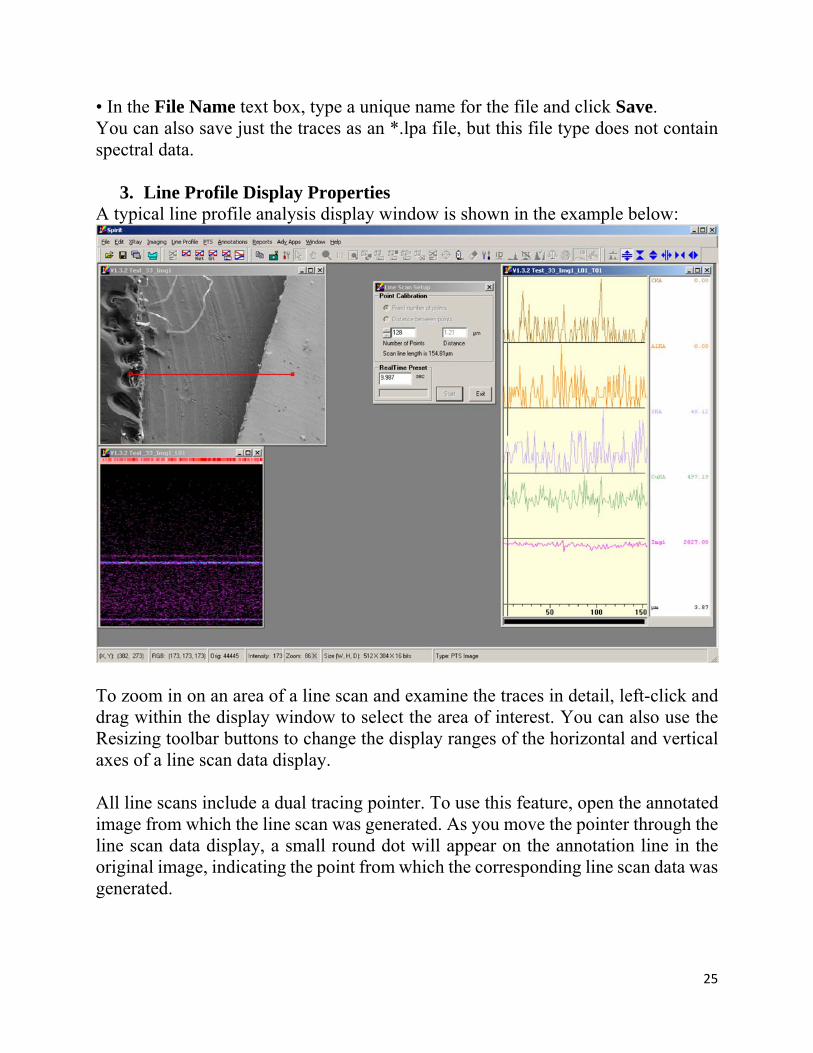
3. Line Profile Display Properties A typical line profile analysis display window is shown in the example below:

To zoom in on an area of a line scan and examine the traces in detail, left-click and drag within the display window to select the area of interest. You can also use the Resizing toolbar buttons to change the display ranges of the horizontal and vertical axes of a line scan data display. All line scans include a dual tracing pointer. To use this feature, open the annotated image from which the line scan was generated. As you move the pointer through the line scan data display, a small round dot will appear on the annotation line in the original image, indicating the point from which the corresponding line scan data was generated.

26  

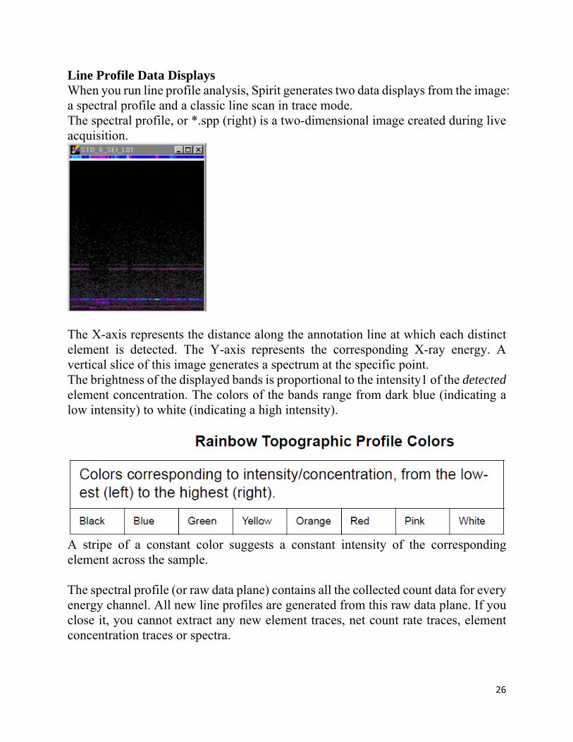
Line Profile Data Displays When you run line profile analysis, Spirit generates two data displays from the image: a spectral profile and a classic line scan in trace mode. The spectral profile, or *.spp (right) is a two-dimensional image created during live acquisition.

The X-axis represents the distance along the annotation line at which each distinct element is detected. The Y-axis represents the corresponding X-ray energy. A vertical slice of this image generates a spectrum at the specific point. The brightness of the displayed bands is proportional to the intensity1 of the detected element concentration. The colors of the bands range from dark blue (indicating a low intensity) to white (indicating a high intensity).

A stripe of a constant color suggests a constant intensity of the corresponding element across the sample. The spectral profile (or raw data plane) contains all the collected count data for every energy channel. All new line profiles are generated from this raw data plane. If you close it, you cannot extract any new element traces, net count rate traces, element concentration traces or spectra.

27  

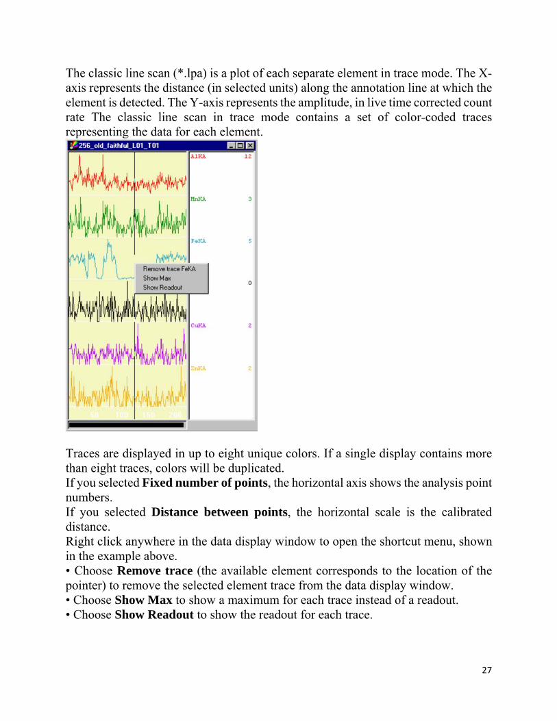
The classic line scan (*.lpa) is a plot of each separate element in trace mode. The X-axis represents the distance (in selected units) along the annotation line at which the element is detected. The Y-axis represents the amplitude, in live time corrected count rate The classic line scan in trace mode contains a set of color-coded traces representing the data for each element.

Traces are displayed in up to eight unique colors. If a single display contains more than eight traces, colors will be duplicated. If you selected Fixed number of points, the horizontal axis shows the analysis point numbers. If you selected Distance between points, the horizontal scale is the calibrated distance. Right click anywhere in the data display window to open the shortcut menu, shown in the example above. • Choose Remove trace (the available element corresponds to the location of the pointer) to remove the selected element trace from the data display window. • Choose Show Max to show a maximum for each trace instead of a readout. • Choose Show Readout to show the readout for each trace.

28  

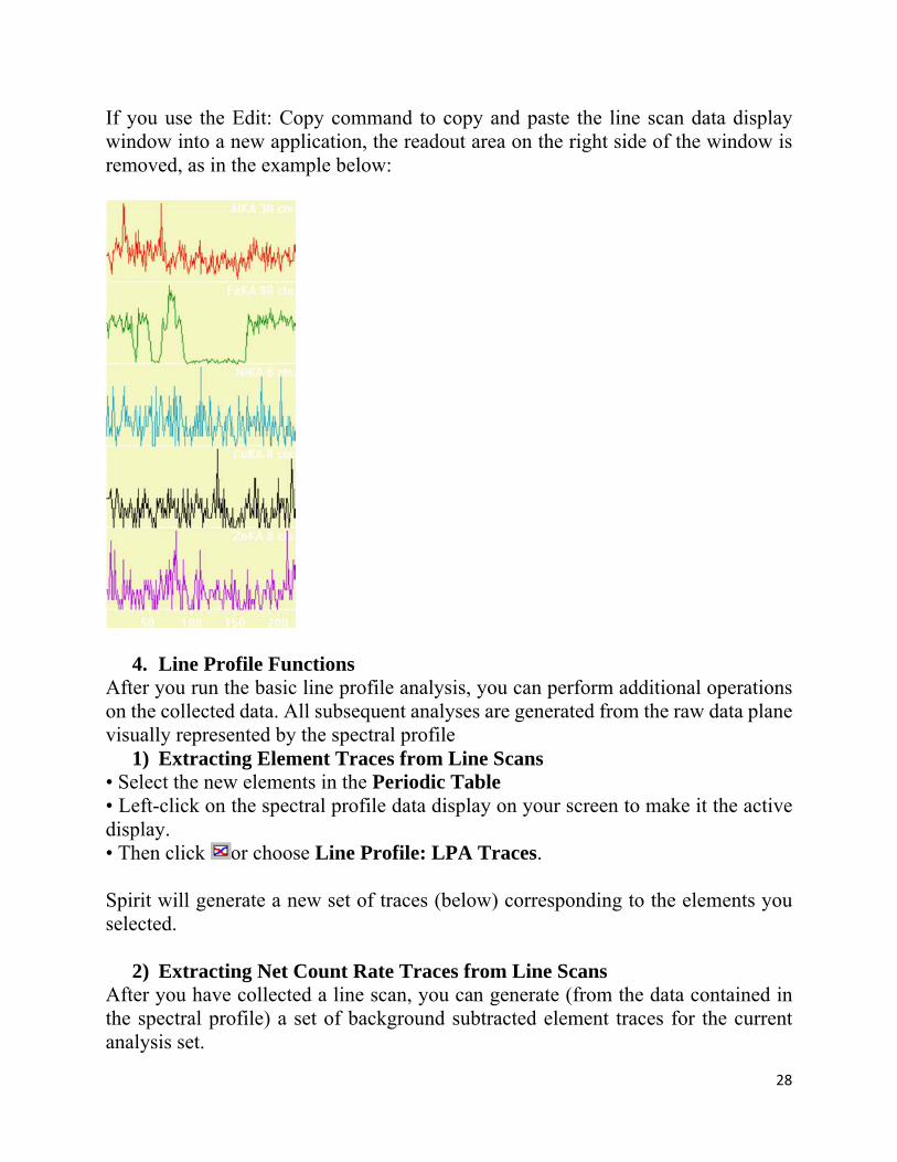
If you use the Edit: Copy command to copy and paste the line scan data display window into a new application, the readout area on the right side of the window is removed, as in the example below:

4. Line Profile Functions After you run the basic line profile analysis, you can perform additional operations on the collected data. All subsequent analyses are generated from the raw data plane visually represented by the spectral profile

1) Extracting Element Traces from Line Scans • Select the new elements in the Periodic Table • Left-click on the spectral profile data display on your screen to make it the active display. • Then click or choose Line Profile: LPA Traces. Spirit will generate a new set of traces (below) corresponding to the elements you selected.

2) Extracting Net Count Rate Traces from Line Scans After you have collected a line scan, you can generate (from the data contained in the spectral profile) a set of background subtracted element traces for the current analysis set.

29  

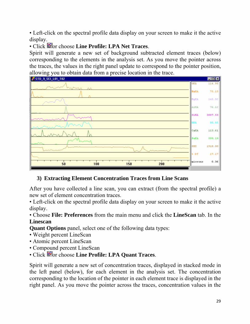
• Left-click on the spectral profile data display on your screen to make it the active display. • Click or choose Line Profile: LPA Net Traces. Spirit will generate a new set of background subtracted element traces (below) corresponding to the elements in the analysis set. As you move the pointer across the traces, the values in the right panel update to correspond to the pointer position, allowing you to obtain data from a precise location in the trace.

3) Extracting Element Concentration Traces from Line Scans

After you have collected a line scan, you can extract (from the spectral profile) a new set of element concentration traces. • Left-click on the spectral profile data display on your screen to make it the active display. • Choose File: Preferences from the main menu and click the LineScan tab. In the Linescan Quant Options panel, select one of the following data types: • Weight percent LineScan • Atomic percent LineScan • Compound percent LineScan • Click or choose Line Profile: LPA Quant Traces.

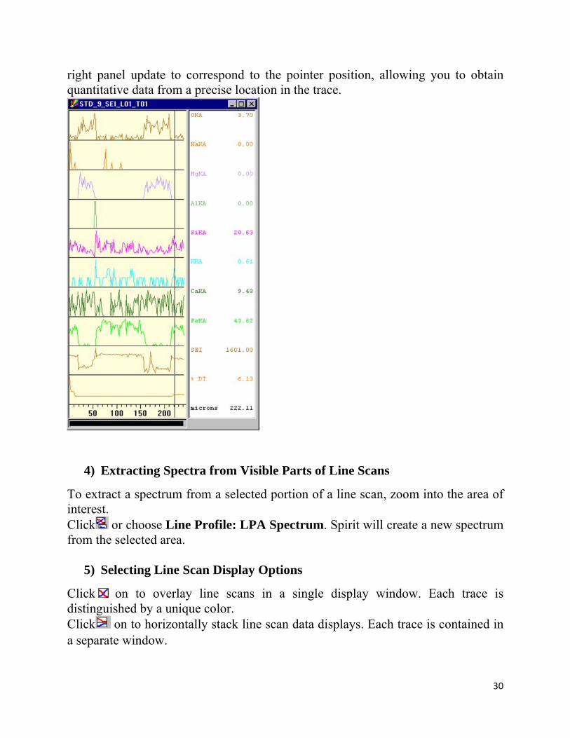
Spirit will generate a new set of concentration traces, displayed in stacked mode in the left panel (below), for each element in the analysis set. The concentration corresponding to the location of the pointer in each element trace is displayed in the right panel. As you move the pointer across the traces, concentration values in the

30  

right panel update to correspond to the pointer position, allowing you to obtain quantitative data from a precise location in the trace.

4) Extracting Spectra from Visible Parts of Line Scans

To extract a spectrum from a selected portion of a line scan, zoom into the area of interest. Click or choose Line Profile: LPA Spectrum. Spirit will create a new spectrum from the selected area.

5) Selecting Line Scan Display Options

Click on to overlay line scans in a single display window. Each trace is distinguished by a unique color. Click on to horizontally stack line scan data displays. Each trace is contained in a separate window.

31  

6) Linescan Overlay The Linescan Overlay display feature allows you to place a copy of a linescan (in overlaid or stacked mode) directly on the corresponding annotation line in the image of origin. Placing a Linescan Overlay on an Image

After acquire a line profile. • Click in the title bar of the image containing the annotation. • Choose Line Profile: Linescan Overlay from the main menu to place the linescan overlay directly on the image.