Semiannual Variation of Geomagnetic Activity · 94 RUSSELL AND MCP•ERRON: SEMIANNUAL VARIATION Although geomagnetic indices such as the U index of 'Figure 1, Ci, Kp, or Ap provide

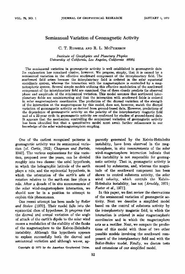
VOL. 78, NO. 1 J'OURNAL OF GEOPHYSICAL RESEARCH •[ANUARY 1, 1973

Semiannual Variation of Geomagnetic Activity

C. T. RUSSELL AND R. L. MCPHERRON

Institute o] Geophysics and Planetary Physics University o] California., Los Angeles, California 9002'4

The semiannual variation in geomagnetic activity is well established in geomagnetic data Its explanation has remained elusive, however. We propose, simply, that it is caused by a semiannual variation in the effective southward component of the interplanetary field. The southward field arises because the interplanetary field is ordered in the solar equatorial coordinate system, whereas the interaction with the magnetosphere is controlled by a-magnetospheric system. Several simple models utilizing this effective modulation of the southward component of the interplanetary field are examined. One of these closely predicts the observed phase and amplitude of the semiannual variation. This model assumes that northward interplanetary fields are noninteracting and that the interaction with southward fields is ordered in solar magnetospheric coordinates. The prediction of the diurnal variation of the strength of the interaction at the magnetopause by this model, does not, however, match the diurnal variation of geomagnetic activity as derived from ground-based data. However, predictions of the dependence of geomagnetic activity on the polarity of the interplanetary magnetic field and of a 22-year cycle in geomagnetic activity are confirmed by studies of ground-based data. It appears that the mechanism controlling the semiannual variation of geomagnetic activity has been identified but that a quantitative model must await further refinements in our knowledge of the solar wind-magnetosphere coupling.

One of the earliest recognized patterns in geomagnetic activity was its semiannual variation [cf. Cottie, 1912; Chapman and Barrels, 1940]. The various explanations for this variation, proposed over the years, can be divided roughly into two classes: the axial hypothesis, in which the heliographic latitude of the earth

,

plays a role, and the equinoctial hypothesis, in which the orientation of the earth's axis of

rotation relative to the earth-sun line plays a role. After a decade of in situ measurements of

the solar: wind-magnetosphere interaction, we should now be in a position to attempt to explain this phenomenon.

One recent attempt has been made by Boiler and Stolov [1970]. Their model falls into the equinoctial class of hypotheses. It proposes that the diurnal and annual variation of the angle of attack of the earth's dipole to the solar wind causes a modulation of the stability of the flanks of the magnetosphere to the Kelvin-Helmholtz instability. Although this hypothesis appears to explain successfully both the diurnal and semiannual variation and although waves, ap-

Copyright ¸ 1973 by the American Geophysical Union.

parently generated by the Kelvin-Helmholtz instability, have been observed in the magnetosphere, in situ measurements of the solar wind-magnetosphere interaction indicate that this instability is not responsible for geomagnetic activity. That is, geomagnetic activity is caused by substorms, and, whereas the magnitude of the southward component has been shown to control substorm activity, the solar wind velocity, which controls the Kelvin- Helmholtz instability, has not [Arnoldy, 1971; Foster et al., 1971].

'In this paper, we first review the observations of the semiannual variation of geomagnetic activity. Next we describe a simplified model based on the control of substorm activity by the interplanetary magnetic field, in which the interaction is ordered in solar magnetospheric coordinates and in which the magnetosphere acts as a rectifier. Next, we compare the predictions of this model with those of two other

possible models involving the southward component of the interplanetary field and with the Boller-Stolov model. Finally, we discuss tests and extensions of our simplified model.

92

I{USSELL AND MCPHERRON: SEMIANNUAL VARIATION

SEMIAN.NUAL VARIATION IN GEOMAGNETIC •an. Feb. •r. Apr. •f•y •un. •. ACTIVITY

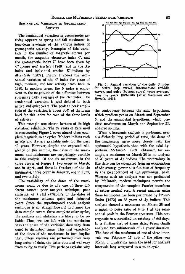
The semiannual variation in geomagnetic activity appears as spring and fall maximums in long-term averages of the various indices of geomagnetic activity. Examples of this variation in the number of magnetic storms per month, the magnetic character index C, and the geomagnetic index U have been given by Chapman and Barrels [1940] and in the Ap index and individual station K indices by Mcintosh [1959]. Figure I shows the semiannual variation of the U index for years of high, medium, and low activity from 1872 to 1930. In modern terms, the U index is equivalent to the magnitude of the difference between successive daily averages of the Dst index. The semiannual variation .is well defined in both

active and quiet years. The peak to peak ampli- -tude of the variation is about 20% of the mean level for this index for each of the three levels

of activity. This example was chosen because of its high

statistical reliability. The 59 years of data used in constructing Figure I cover almost three complete magnetic solar cycles. Modern indices such as Kp and Ap are available only for the past 40 years. However, despite the expected reliability of this sample, the d•tes of the maximums and minimums are surprisingly variable in this analysis. Of the six maximums, in the three curves of Figure 1, two occur in March, one in April, and three in October; of the six minimums, three occur in January, one in June, and two in July.

The variability of the dates of the maximums could be due to any one of three different causes: poor analytic technique, poor statistics, or a real variability of the dates of the maximums between quiet and disturbed years. Since the superimposed epoch analysis technique is so straightforward and since the data sample covers three complete solar cycles, the analysis and statistics are likely to be re- liable. Thus, we are left with the conclusion that the phase of the variation does vary from quiet to disturbed times. This real variability of the dates of the maximums in turn implies that, unless analyses are performed over very long series Of data, the dates obtained will vary from study to study. This perhaps explains why

801 • ' ' ' J ' ' • ' ' ' ' ' i

7o

•o

9o

93

- ß

I I I I I I I I I I

Fig. 1. Annual variation of the daily U index for active (top curve), intermediate (middle curve), and quiet (bottom curve) years averaged over the years 1872-1930 [after Chapman and Bartels, 1940].

the controversy between the axial hypothesis, which predicts peaks on March and September 5, and the equinoctial hypothesis, which predicts maximums on March and September 21, endured so long.

'When a harmonic analysis is performed over a sufficiently long period of time, the dates of the maximums agree more closely with the equinoctial hypothesis than with the axial hypothesis. Mcintosh [1959] obtained, for example, a maximum on March 28 in an analysis of 20 years of A p indices. The uncertainty in this date can be calculated from an examination

of the average power as a function of frequency in the neighborhood of the semiannual peak. Whereas such an analysis was not performed by Mcintosh, modern techniques permit the computation of the complete Fourier transform at rather modest cost. A recent analysis using these techniques has been performed by Fraser- Smith [1972] on 38 years of Ap indices. This analysis showed a maximum on March 25 and a signal to noise ratio of 6 to I at the semiannual peak in the Fourier spectrum. This corresponds to a statistical uncertainty of --+5 days. In a further test of these data, Fraser-Smith analyzed two subintervals of 11 years' duration. The date of the maximum of one of these inter-

vals was February 17 and-. of the other was March 3, illustrating again the need for analysis intervals long compared to a solar cycle.

94 RUSSELL AND MCP•ERRON: SEMIANNUAL VARIATION

Although geomagnetic indices such as the U index of 'Figure 1, Ci, Kp, or Ap provide an excellent• data base for determining the phase of the semiannual variation, they do not provide a quantitative measure of this modulation. Storm counts, however, can provide a quantitative estimate of the semiannual modulation of energy input to the magnetosphere.

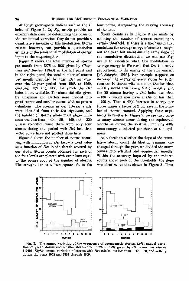
Figure 2 shows the total number of storms per month from 1875 to 1927 given by Chap- man and Barrels [1940] in the left panel and in the right panel the total number of storms per month identified by their Dst signature over the 10-year period from 1958 to 1969, omitting 1959 and 1960, for which the Dst index is not available. The storm statistics given by Chapman and Bartels were divided into great storms and smaller storms with no precise definitions. The storms in our 10-year study were identified from their Dst signature, and the number of storms whose main phase minimum was less than --40, --80, --160, and --320 7 was recorded. Since there were only four storms during this period with Dst less than --320 7, we have not plotted those here.

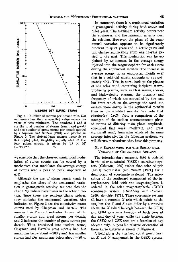
Figure 3 shows the number of storms occurring with minimums in Dst below a fixed value as a function of Dst in the decade covered by our study. Storm counts obtained for each of the four levels are plotted with error bars equal to the square root of the number of storms. The straight line is a least squares fit to the

four points, disregarding the varying accuracy of the data.

Storm counts as in Figure 2 are made by counting the number of storms exceeding~a certain threshold. If there is a mechanism that

modulates the average energy of storms throughout the year but maintains the same slope of the cumulative distribution, we can use Fig- ure 3 to calculate what this modulation in

average energy is. We recall that Dst is directly proportional to the energy of the ring current [cf. $ckopke, 1966]. For example, suppose we increased the energy of every storm by 40%; then the 10 storms with minimum Dst less than

--200 7 would now have a Dst of --280 7, and the 20 storms having a Dsi index less than --160 7 would now have a Dst of less than --200 7. Thus a 40% increase in energy per storm causes a factor of 2 increase in the num-

ber of storms counted. Applying these argu- ments in reverse to Figure 2, we see that twice as many storms occur during the equinoctial months as during the solstitial, implying 40% more energy is injected per storm at the equinoxes.

As a check on whether the slope of the cumulative storm count distribution remains un-

changed through the year, we divided the storm counts into solstitial and equinoctial months. Within the accuracy imposed by the reduced counts above each of the thresholds, the slope was identical to that shown in Figure 3. Thus,

o- 40 - 4o

, ,

• SMALLER STORMS •

rr 20 _• 20 ß z • .

I o .• GREAT I o

ß

0 , , "' 'i ....... i ..... i ...... , .... i , '"'i ....... i .... • ..... 0

I 2 3 4 õ 6 ? 8 9 I0 II 12 I 2 3 4 õ 6 ? 8 9 I0 II

MONTH MONTH

Fig. 2. The annual variation of the occurrence of geomagnetic storms. Le/t: annual variation of great storms and smaller storms from 1875 to 1927 give• by Chapman and Bartels [ 1940]. Right: annual variation of storms with Dst minimums less than --40, .--80, and --160 7 during the years 1958 and 1961 through 1969.

RUSSELL AND MCPHERRON' SEMI*•VAL VARIA?IO• 95

ioo -- -

-

-

-

-

-

I0-- -

-

.

-

_

-

i i i i i i I i i i i i i I I 1 _

I i i •

- io -ioo -iooo

MINIMUM DST DURING STORM

Fig. 3. Number of storms per decade with Dst minimums less than a specified value versus the value of this minimum. The numbers 1 and 2 are the total number of storms (smal! and great) and the number of great storms per decade quoted by Chapman and Bartels [1940] and plotted in Figure 2. The plotted least squares linear fit to this log-log plot, weighting equally each of the four points shown, is given by 1.7 X 106 (--Dst )-•'•. • !

we conclude that the observed semiannual modu-

lation of storm counts can be caused by a mechanism that modulates the average energy of storms with a peak to peak amplitude of 40%.

Although the use of storm counts tends to emphasize the effect of the semiannual variation in geomagnetic activity, we note that the C and Kp indices have biases in the other direction. Since these are semilogarithmic indices, they minimize the semiannual variation. Also indicated on Figure 3 are the cumulative storm counts used by Chapman and Barrels. The number 1 in Figure 3 indicates the sum of the smaller storms and great storms per decade, and 2 indicates the number of great storms per decade. Thus, translated into modem terms, Chapman and Bartel's great storms had Dst mi•iimums below about -200 y and their smaller' storms had Dst minimums below about -80 y.

In summary, there is a semiannual variation in geomagnetic activity during both active and quiet years. The maximum activity occurs near the equinoxes., and *_.he minimum activity near the solstices. However, the phase of the semiannual variation appears to be significantly different in quiet years and in active years and can change significantly from one 11-year period to the next. This modulation can be ex-

plained by an increase in the average energy injected into the magnetosphere for each storm during the equinoctial months. The increase in average energy in an equinoctial month over that in a solstitial month amounts to approximately 40%. This, in turn, leads to the picture of the solar wind containing incipient storm- producing plasma, such as blast waves, shocks, and high-velocity streams, the intensity and frequency of which are controlled by the sun, but from which on the average the earth can extract more energy in the equinoctial months than in the solstitial months. We note that

Piddington [1963], from a comparison of the strength of the sudden commencement phase of storms of differing main phase amplitude, concluded that weak, moderate, and great storms all result from solar winds of the same

average intensity. In the following sections, we will discuss mechanisms that have this property.

NEW EXPLANATION FOR THE SEMIANNUAL

VARIATION OF GEOMAGNETIC ACTIVITY

The interplanetary magnetic field is ordered in the solar equatorial (GSEQ) coordinate system [Coleman, 1966] rather than solar ecliptic (GSE) coordinates (see Russell [1971] for a description of coordinate systems). The interaction of the southward component of the interplanetary field with the magnetosphere is ordered in the solar magnetospheric (GSM) coordinate system [Hirshberg and Colburn,

1969; Arnold.y, 1971]. These coordinate systems all have a common X axis which points at the sun, but the Y and Z axes differ by a rotation about the X axis. The angle between the GSEQ and GSM axes is a function of both time of

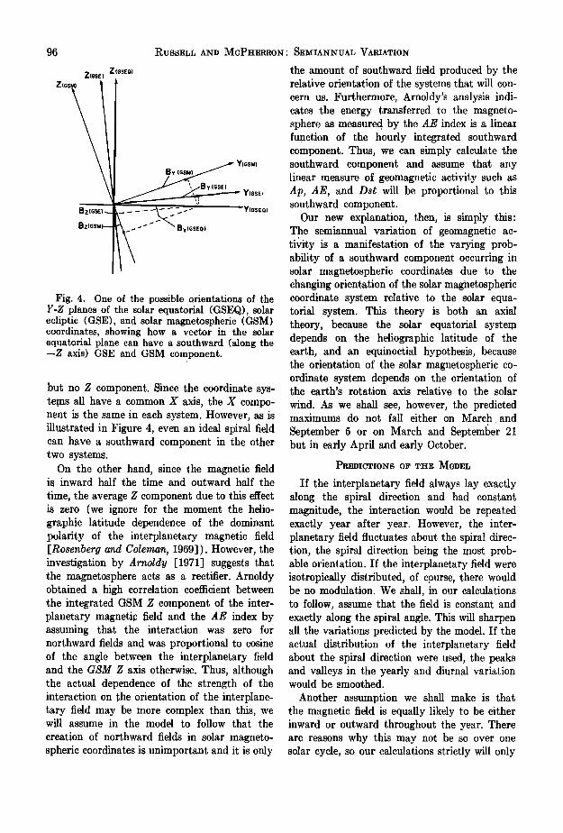
day and day of year, while the angle between the GSEQ and GSE axes are a function of day of-year only. A possible relative orientation of these three systems is shown in Figure 4.

A field along the idealized spiral would have an X and Y component in the GSEQ system,

96 RUSSELL AND McP•IERRON: SEmIANNUaL V•RI•T•ON

Z(•sœ) Z Z(GS

Y(GSM) E•y (GSM)

Y(GSE,

BZ(GSM)

Fig. 4. One of the possible orientations of the Y-Z planes of the solar equatorial (GSEQ), solar ecliptic (GSE), and solar magnetospheric (GSM) coo.rdinates, showing how a vector in the solar equatorial plane can have a southward (along the --Z axis) GSE and GSM component.

but no Z component. Since the coordinate systems all have a common X axis, the X component is the same in each system. However, as is illustrated in Figure 4, even an ideal spiral field can have a southward component in the other two systems.

On the other hand, since the magnetic field is inward half the time and outward half the

time, the average Z component due to this effect is zero (we ignore for the moment the heliographic latitude dependence of the dominant polarity of the interplanetary magnetic field [Rosenberg and Coleman, 1969] ). However, the investigation by Arnoldy [1971] suggests that the magnetosphere acts as a rectifier. Arnoldy obtained a high correlation coefficient between the integrated GSM Z component of the interplanetary magnetic field and the AE index by assuming that the interaction was zero for northward fields and was proportional to cosine of the angle between the interplanetary field and the GSM Z axis otherwise. Thus, although the actual dependence of the strength of the interaction on .the orientation of the interplanetary field may be more complex than this, we will assume in the model to follow that the

creation of northward fields in solar magnetospheric coordinates is unimportant and it is only

the amount of southward field produced by the relative orientation of the systems that will con- cern us. Furthermore, Arnoldy's analysis indicates the energy transferred to the magnetosphere as measured by the AE index is a linear function of the hourly integrated southward component. Thus, we can simply calculate the southward component and assume that any linear measure of geomagnetic activity such as Ap, AE, and Ds• will be proportional to this southward component.

Our new explanation, then, is simply this: The semiannual variation of geomagnetic activity is a manifestation of the varying probability of a southward component occurring in solar magnetospheric coordinates due to the changing orientation of the solar magnetospheric coordinate system relative to the solar equatorial system. This theory is both an axial theory, because the solar equatorial system depends on the heliographi½ latitude of the earth, and an equinoctial hypothesis, because the orientation of the solar magnetospheric coordinate system depends on the orientation of the earth's rotation axis relative to the solar

wind. As we shall see, however, the predicted maximums do not fall either on March and

September 5 or on March and September 21 but in early April and early October.

PREDICTIONS OF TI-IE MODEL

If the interplanetary field always lay exactly along the spiral direction and had constant magnitude, the interaction would be repeated exactly year after year. However, the interplanetary field fluctuates about the spiral direction, the spiral direction being the most prob- able orientation. If the interplanetary field were isotropically distributed, of cpurse, there would be no modulation. We shall, in our calculations to follow, assume that the field is constant and exactly along the spiral angle. This will sharpen all the variations predicted by the model. If the actual distribution of the interplanetary field about the spiral direction were used, the peaks and valleys in the yearly and diurnal variation would be smoothed.

Another assumption we shall make is that the magnetic field is equally likely to be either inward or outward throughout the year. There are reasons why this may not be so over one solar cycle, so our calculations strictly will only

RUSSELL AND MCPHERRON

apply to averages over two or more solar cycles. We shall discuss the effect of the heliographic latitude dependence of the dominant polarity later in this paper. Finally, we assume for our calculations that northward interplanetary fields are noninteracting and that the interaction with the southward-directed fields is linearly proportional to the size of the southward component.

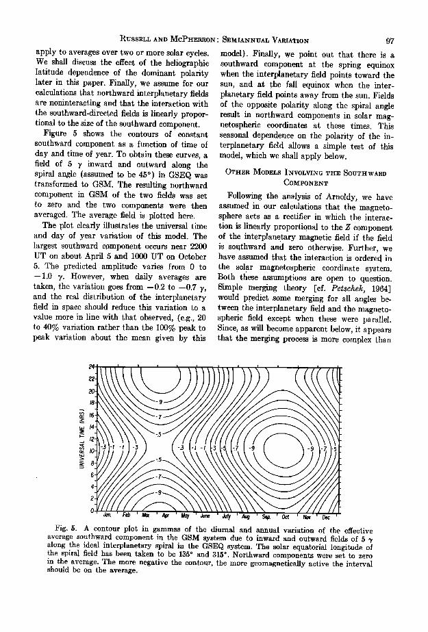
Figure 5 shows the contours of constant southward component as a function of time of day and time of year. To obtain these curves, a field of 5 y inward and outward along the spiral angle (assumed to be 45 ø) in GSEQ was transformed to GSM. The resulting northward component in GSM of the two fields was set to zero and the two components were then averaged. The average field is plotted here.

The plot clearly illustrates the universal time and day of year variation of this model. The largest southward component occurs near 2200 UT on about April 5 and 1000 UT on October 5. The predicted amplitude varies from 0 to --1.0 y. However, when daily averages are taken, the variation goes from -0.2 to --0.7 7, and the real distribution of the interplanetary field in space should reduce this variation to a value more in line with that observed, (e.g., 20 to 40% variation rather than the 100% peak to peak variation about the mean given by this

: SEMIANNUAL VARIATION 97

model). Finally, we point out that there is a southward component at the spring equinox when the interplanetary field points toward the sun, and at the fall equinox when the interplanetary field points away from the sun. Fields of the opposite polarity along the spiral angle result in northward components in solar magnetospheric coordinates at these times. This seasonal dependence on the polarity of the interplanetary field allows a simple test of this model, which we shall apply below.

OTI-IER MODELS INVOLVING TI-IE SOUTI-IWARD COMPONENT

Following the analysis of Arnoldy, we have assumed in our calculations that the magnetosphere acts as a rectifier in which the interaction is linearly proportional to the Z component of the interplane. tary magnetic field if the field is southward and zero otherWise. Further, we have assumed that the interaction is ordered in the solar magnetospheric coordinate system. Both t•ese assumptions are open to question. Simple merging theory [cf. Petschelc, 1964] would predict some merging for all angles between the interplanetary field and the magnetospheric field except when these were parallel. Since, as will become apparent below, it appears that the merging process is more complex than

zo- /

Is: •-• /

• i0 • '..' • I I

6 •

0 on. ' Feb. ' Mot. Apr. •f• ' :une ' :Ul, Aug ' $ep ' Oct. ' qov • •)ec ' •ig. 5. • contour plot in gammas of the diu•al and annual variation of the effective

average southward component in the G•M system due to inward and outward fields of 5 '• along the ideal interplanetary spiral in the GSEQ system. The solar equatorial longitude of the spiral field has been taken to be 135 ø and 315 ø . Northward components were set to zero in the average. The more negative the contour, the more geomagnetically active the interval should be on the average.

98 RUSSELL AND McPI-IERRON: SEMIANNUAL VARIATION

this, we shall refer to this model as the simple merging model.

The assumption that the solar magnetospheric coordinate system orders the interaction has been tested by Hirshberg and Colburn [1969] and Arnoldy [1971] only to the extent that it orders the interaction to a higher degree than the solar ecliptic coordinate system. A com- peting system, the solar magnetic coordinate system, has not been tested. In this section, we will relax these two assumptions and examine two alternative models involving the southward component of the interplanetary magnetic field.

Simple merging model. In the preceding model, we assumed that the interaction was zero for a northward-pointing field. However, naively we might expect merging to occur at the nose of the magnetosphere whenever the magnetospheric field and the interplanetary field were not exactly aligned. This merging may be thought of as due to an effective southward component. Figure 6 shows how this arises.

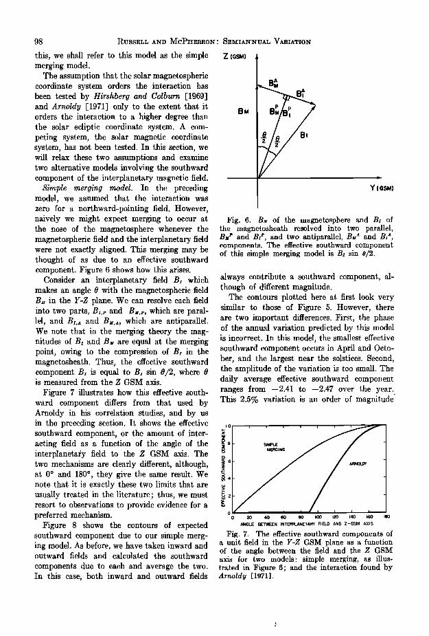
Consider an interplanetary field B• which makes an angle • with the magnetospheric field B• in the Y-Z plane. We can resolve each field into two parts, B•.p and B•,•,, which are parallel, and B•,a and B•.•, which are antiparallel. We note that in the merging theory the mag- nitudes of B• and B• are equal at the merging point, owing to the compression of B• in the magnetosheath. Thus, the effective southward component B• is equal to B• sin 0/2, where 0 is measured from the Z GSM axis.

Figure 7 illustrates how this effective southward component differs from that used by Arnoldy in his correlation studies, and by us in the preceding section. It shows the effective southward component, or the amount of inter- acting field as a function of the angle of the interplanetary field to the Z GSM axis. The two mechanisms are clearly different, although, at 0 ø and 180 ø, they give the same result. We note that it is exactly these two limits that are usually treated in the literature; thus, we must resort to observations to provide evidence for a preferred mechanism.

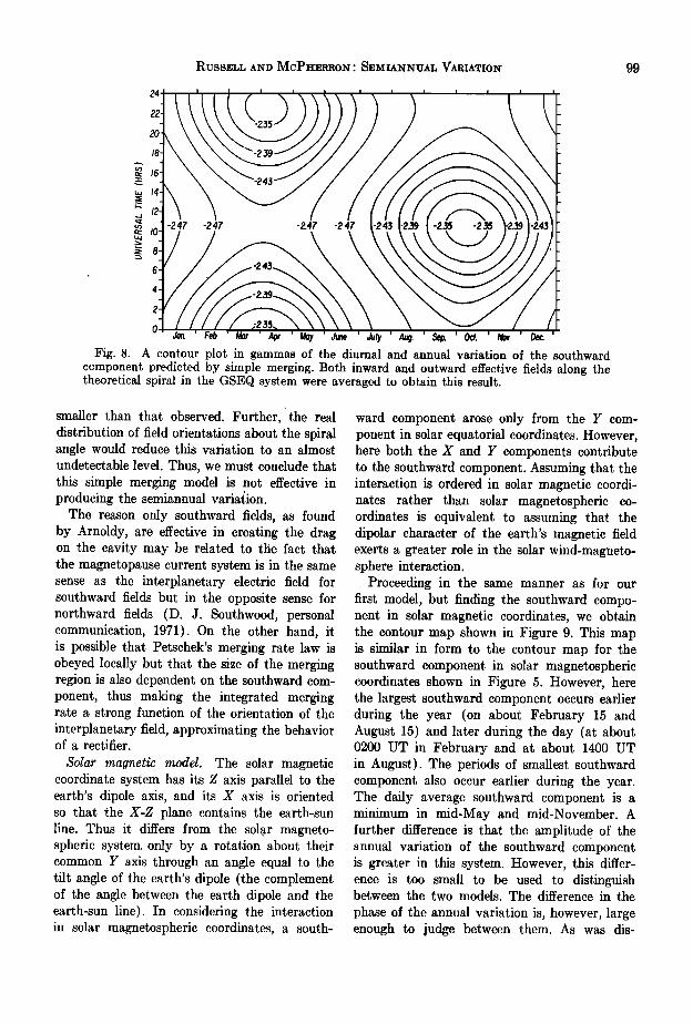
Figure 8 shows the contours of expected southward component due to our simple merging model. As before, we have taken inward and outward fields and calculated the southward

components due to each and average the two. In this case, both inward and outward fields

Z (GSM)

aM

Y (GSM)

Fig. 6. B• of the magnetosphere and B• of the magnetosheath resolved into two parallel, B• • and B• •, and two antiparallel, B• • and B• •, components. The effective southward component of this simple merging model is B• sin e/2.

always contribute a southward component, although of different magnitude.

The contours plotted here at first look very similar to those of Figure 5. However, there are two important differences. First, the phase of the annual variation predicted by this model is incorrect. In this model, the smallest effective southward component occurs in April and Octo- ber, and the largest near the solstices. Second, the amplitude of the variation is too small. The daily average effective southward component ranges from --2.41 to --2.47 over the year. This 2.5% variation is an order of magnitude

MERGING

_

0 0 20 40 60 80 I00 120 140 160

ANGLE BETWEEN INTERPLANETARY FIELD ANO Z-GSM AXIS

Fig. 7. The effective southward components of a unit field in the Y-Z GSM plane as a function of the angle between the field and the Z GSM axis for two models: simple merging, as illustrated in Figure 6; and the interaction found by Arnoldy [1971].

RUSSELL AND MCPHERRON: SEMIANNUAL VARIATION 99

74 I / I i i I

c• 16-

•: I0

_

0 , .... • Sep ' Oct ' • ' • '

•g. 8. • co.tour plo[ • g•mma• of •he d•umal and compo•e• pred•c[ed by s•mp]e merging. •o•h •w•rd •d outward effective fields along the •heorefic•l •p•r•] • •he •• •ys•em were •ver•ged •o obLa• [h•s

smaller than that observed. Further, the real distribution of field orientations about the spiral angle would reduce this variation to an almost undetectable level. Thus, we must conclude that this simple merging model is not effective in producing the semiannual varia{ion.

The reason only southward fields, as found by Arnoldy, are effective in creating the drag on the cavity may be related to the fact that the magnetopause current system is in the same sense as the interplanetary electric field for southward fields but in the opposite sense for northward fields (D. J. Southwood, personal communication, 1971). On the other hand, it is possible that Petschek's merging rate law is obeyed locally but that the size of the merging region is also dependent on tke southward component, thus making the integrated merging rate a strong function of the orientation of the interplanetary field, approximating the behavior of a rectifier.

Solar magnetic model. The solar magnetic coordinate system has its Z axis parallel to the earth's dipole axis, and its X axis is oriented so that the X-Z plane contains the earth-sun line. Thus it differs from the solar magnetospheric system. only by a rotation about their common Y axis through an angle equal to the tilt angle of the earth's dipole (the complement of the angle between the earth dipole and the earth-sun line). In considering the interaction in solar magnetospheric coordinates, a south-

ward component arose only from the Y component in solar equatorial coordinates. However, here both the X and Y components contribute to the southward component. Assuming that the interaction is ordered in solar magnetic coordinates rather than solar magnetospheric coordinates is equivalent to assuming that the dipolar character of the earth's magnetic field exerts a greater role in the solar wind-magnetosphere interaction.

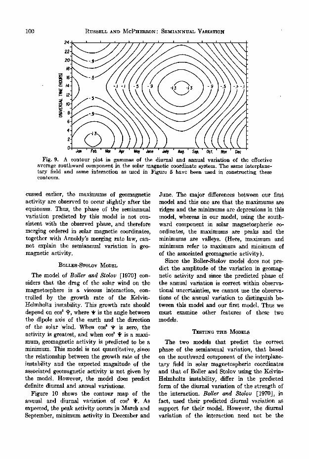
Proceeding in the same manner as for our first model, but finding the southward component in solar magnetic coordinates, we obtain the contour map shown in Figure 9. This map is similar in form to the contour map for the southward component in solar magnetospheric coordinates shown in Figure 5. However, here the largest southward component occurs earlier during the year (on about February 15 and August 15) and later during the day (at about 0200 UT in February and at about 1400 UT in August). The periods of smallest southward component also occur earlier during the year. The daily average southward component is a minimum in mid-May and mid-November. A further difference is that the amplitude of the annual variation of the southward component is greater in this system. However, this difference is too small to be used to distinguish between the two models. The difference in the

phase of the annual variation is, however, large enough to judge between them. As was dis-

100 RUSSELL AND MCPHERRON: SEMIANNUAL VARIATION

t9•d I I I . I I I I I I I I I I

0 Moy 'June ' ' ' Od. ' Nov. ' Dec. ' July 'Aug. $ep.

Fig. 9. A contour plot in gammas of the diurnal and annual variation of the effective average southward component in the solar magnetic coordinate system. The same interplanetary field and same interaction as used in Figure 5 have been used in constructing these contours.

cussed earlier, the maximums of geomagnetic activity are observed to occur slightly after the equinoxes. Thus, the phase of the semiannual variation predicted by this model is not consistent with the observed phase, and therefore merging ordered in solar magnetic coordinates, together with Arnoldy's merging rate law, cannot explain the semiannual variation in geomagnetic activity.

•BOLLER-STOLOV MODEL

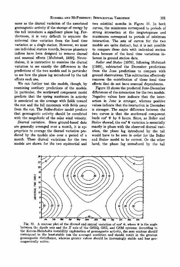
The model of Bullet a•d Stolov [1970] con- siders that the drag of the solar wind on the magnetosphere is a viscous interaction, controlled by the growth rate of the Kelvin- Helmholtz instability. This growth rate should depend on cos •' •, where ß is the angle between the dipole axis of the earth and the direction of the solar 'wind. When cos •' • is zero, the activity is greatest, and when cos 2 • is a maximum, geomagnetic activity is predicted to be a minimum. This model is not quantitative, since the relationship between the growth rate of the instability and the expected magnitude of the associated geomagnetic activity is not given by the model. However, the model does predict definite diurnal and annual variations.

Figure 10 shows the contour map of the annual and diurnal variation of cos •' •. As

expected, the peak activity occurs in March and September, minimum activity in December and

June. The major differences between our first model and this one are that the maximums are

ridges and the minimums are depressions in this model, whereas in our model, using the southward component in solar magnetospheric coordinates, the maximums are peaks and the minimums are valleys. (Here, maximum and minimum refer to maximum and minimum of

of the associated geomagnetic activity).. Since the Boller-Stolov model does not pre-

dict the amplitude of the variation in geomagnetic activity and since the predicted phase of the annual variation is correct within observa-

tional uncertainties, we cannot use the observations of the annual variation to distinguish between this model and our first model. Thus we must examine other features of these two models.

TESTING THE MODELS

The two models that predict the correct phase of the semiannual variation, that based on the southward component of the interplanetary field in solar magnetospheric coordinates and that of Boller and Stolov using the Kelvin- Helmholtz instability, differ in the predicted form of the diurnal variation of the strength of the interaction. Boller and Stolov [1970], in fact, used their predicted diurnal variation as support for their model. However, the diurnal variation of the interaction need not be the

RUSS•,LL AND McPH•,RRON: SEMIANNUAL VARIATION 101

same as the diurnal variation of the associated

geomagnetic activity if the storage of energy by the tail introduces a significant phase lag. Fur- thermore, it is very difiqcult to separate the universal time variation from the local time

variation at a single station. However, we must use individual station records, because planetary indices have been designed to remove diurnal and seasonal effects [Mcintosh, 1959]. Never- theless, it is instructive to examine the diurnal variation to see exactly the differences in the predictions of the two models and in particular to see how the phase lag introduced by the tail affects each one.

We can further test the models, though, by examining auxiliary predictions of the models. In particular, the southward component model predicts that the spring maximum in activity is associated on the average with fields toward the sun and the fall maximum with fields away from the sun. The Boller-Stolov model predicts that geomagnetic activity should be correlated with the magnitude of the solar wind velocity.

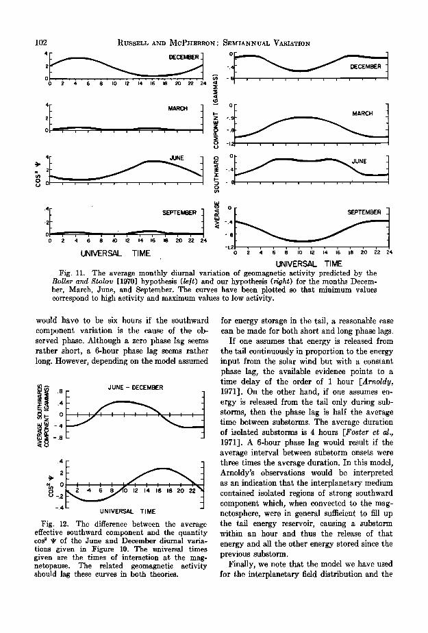
Diurnal variation. Since ground-based data are generally averaged over a month, it is ap- propriate to average the diurnal variation predicted by the models also over a period of a month. These diurnal variations for the two

models are shown for the two equinoctial and

two solstitial months in Figure 11. In both curves, the minimums correspond to periods of strong interaction at the magnetopause and maximums correspond to periods of minimum interaction. The sets of curves for the two

models are quite distinct, but it is not possible to compare these data with individual station data because of the local time variations in-

herent in ground station data. Boller and Stolov [1970], following Mcintosh

[1959], subtracted the December predictions from the June predictions to compare with ground observations. This subtraction effectively removes the contribution of those local time

effects that do not have seasonal dependences. Figure 12 shows the predicted June-December

differences of the interaction for the two models.

Negative values here indicate that the interaction in June is stronger, whereas positive values indicate that the interaction in December

is stronger. The major difference between the two curves is that the southward component leads cos • i by 6 hours. Since, as Boller and Stolov showed, the cos '• i variation is essentially exactly in phase with the observed diurnal variation, the phase lag introduced by the tail would have to be zero in order for the Boller and Stolov model to be correct. On the other

hand, the phase lag introduced by the tail

Fig. 10. A contour plot of the diurnal and annual variation of cos • •, where ß is the angle between the dipole axis and the X axis of the GSEQ, GSE, and GSM systems. According to the Kelvin-Helmholtz instability explanation of geomagnetic activity, the zero contour should correspond to the least-stable (on the average) condition and should result in the greatest geomagnetic disturbance, whereas greater values should.be increasingly stable and less geomagnetically active.

102 R•SSELL A•D McPHERRO•' SE•A••L V•R•?•o•

'0 •E•E• -. DECEMiR 0 2 4 6 8 I0 12 14 16 18

ß • - 9 MARCH

'. ' I

,, , o

• 0 ß 4 SEPTE•ER

0 -.8 0 2 4 6 8 I0 12 14 16 18 20 22 24

'1.2• , • • I , • , • •

UNIVERSAL TIME o 2 4 6

UNIVERSAL TIME •J•. 11. The average monthly dJum•] v•rJ•tJo• of •eom•etJc •cfivJty predicted by the

Bo•er • •o•o• [1970] hypothes•s (JeJ•) •d our hypothes•s (•g•) for the mo•ths Decem- her, •rch, Ju•e, •d September. The curves h•ve bee• plotted so •h•[ minimum v•]ues correspond to high •ctivity •d maximum v•]ues to low

would have to be six hours if the southward

component variation is the cause of the observed phase. Although a zero phase lag seems rather short, a 6-hour phase lag seems rather long. However, depending on the model assumed

•-! .8 JUNE - DECEMBER o

.4

-.4 •'• I• I• 16 18 20 UNIVERSAL TIME

Fig. 12. The difference between the average effective southward component and the quantity cos • ß of the June and December diurnal varia-

tions given in Figure 10. The universal times given are the times of interaction at the magnetopause. The related geomagnetic activity should lag these curves in both theories.

for energy storage in the tail, a reasonable case can be made for both short and long phase lags.

If one assumes that energy is released from the tail continuously in proportion to the energy input from the solar wind but with a constant phase lag, the available evidence points to a time delay of the order of I hour [Arnoldy, 1971]. On the other hand, if one assumes energy is released from the tail only during substorms, then the phase lag is half the average time between substerms. The average duration of isolated substerms is 4 hours [Foster et al., 1971]. A 6-hour phase lag would result if the average interval between substerm onsets were three times the average duration. In this model, Arnoldy's observations would be interpreted as an indication that the interplanetary medium contained isolated regions of strong southward component which, when convected to the magnetosphere, were in general sufficient to fill up the tail energy reservoir, causing a substerm within an hour and thus the release of that

energy and all the other energy stored since the previous substerm.

Finally, we note that the model we have used for the interplanetary field distribution and the

RUSSELL AND MCPYIERRON.' SEMIANNUAL VARIATION 103

interaction of the interplanetary field with the causative effect of the solar wind velocity on magnetosphere are approximations. Use of the geomagnetic activity but are probably due to real distribution of the interplanetary field and the intercorrelation of the solar wind param- an improved knowledge of the dependence of eters. the interaction on the orientation of the field Since we have based our model on the ob- could alter the phase of the diurnal variation served dependence of geomagnetic activity on and the annual variation somewhat without the southward component of the interplanetary altering the basic mechanism. Fortunately, there magnetic field, we cannot use the observation are some qualitative tests that depend pri- of this dependence as an additional test. How- marily on the mechanism and not on a precise ever, in section 4, we noted that the southward definition of a date which depends on details of component in our model during the spring a model. equinox occurred when the interplanetary field

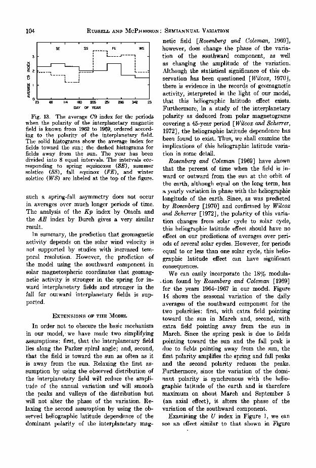
Auxiliary predictions o• the models. An aux- was toward the sun, and the southward com- iliary prediction of the model of Boller and ponent during the fall equinox occurred when Stolov is that geomagnetic activity will be a the interplanetary field was away from the sun. function of the magnitude of the solar wind Thus, an auxiliary prediction of the model is velocity. A positive correlation between the that, if geomagnetic activity is separated ac- solar wind velocity and Kp has been found cording to the polarity of the interplanetary [Snyder et al., 1963; Wilcox et al., 1967]. How- field, the semiannual variation will be split into ever, the solar wind velocity was also found to two annual variations: one with a spring maxi- be a rather poor predictor of Kp. For example, mum for fields toward the sun and one with a at a solar wind velocity of 300 km/sec, the fall maximum for fields away from the sun. Kp index could range from 0 to 5. Further- Both J. A. Otaola and G. L. Siscoe (personal more, the relationships found by Snyder et al. communications, 1971) have independently ex- and Wilcox et al. were significantly different, amined the dependence of the annual variation and, finally, Wilcox et al. found that other solar of geomagnetic activity on the polarity of the wind parameters, for example, the interplane- interplanetary field. J. A. Otaola examined the taw field magnitude, correlated as well as the variation of the Kp index, and G. L. Siscoe solar wind velocity. Hirshberg'and Colburn examined the variation of the C9 index. More [1969] have suggested that the above situation recently, Burch [1972] has studied this effect in arises because, while there may be only one the AE index. causative agent of geomagnetic activity in the Figure 13 shows the diurnal variation of the solar wind, the solar wind parameters them-. average C9 index, follov•ing the analysis of selves are highly correlated. Siscoe. The polarity of the field and the C9

More recent studies [Arnoldy, 1971; Foster index have been obtained from the chart given eta/., 1971], on the other hand, have given by Wilcox and Colburn [1970]. The year has evidence that the southward component of the been divided into 8 equal intervals centered on interplanetary field is the causative agent of the equinoxes and solstices. We see that the geomagnetic activity. These studies gave un- presently available data do follow the trend ambiguous results despite the correlations be- predicted by our model. The variation of ac- tween the various solar wind parameters, be- tivity for both polarities is predominantly an cause these recent studies were based on high annual variation rather than a semiannual vari- time resolution data. An examination o• the ation. The peak activity for fields toward the results presented by both Arnoldy and by sun occurs in the spring and the peak activity Foster et al. shows that, if they had used 3- for fields away from the sun occurs in the fall. hour averages as did Snyder et al. and Wilcox Since the data used in this study cover less et al., the observed correlations with the south- than one solar cycle, we would expect depar- ward component would have been much weaker. tures from the predictions of our model due to

Thus, in the light of recent studies, it appears the statistical nature of geomagnetic activity. that the previously found correlations between Such departures are readily apparent. In par- geomagnetic activity and solar wind velocity, ticular, the fall equinox during this period was although real, do not necessarily stem from a far more active than the spring equinox, whereas

104 RUSSELL AND McPIIERRON' SEMIANNUAL VARIATION

i i

$

0 25 68

!

r- .... -'1 !

I t ..... I

', I

i !

FE WS

_r' .... '1 !

I

I

I I I I I I

114 160 205 251 296 •42 2•

DAY OF YEAR

Fig. 13. The average C9 index for the periods when the polarity of the interplanetary magnetic field is known from 1962 to 1969, ordered according to the polarity of the interplanetary field. The solid histograms show the average index for fields toward the sun; the dashed histograms for fields away from the sun. The year has been divided into 8 equal intervals. The intervals cor- responding to spring equinoxes ($E), summer solstice (SS), fall equinox (FE), and winter solstice (WS) are labeled at the top of the figure.

such a spring-fall asymmetry does not occur in averages over much longer periods of time. The analysis of the Kp index by 0taola and the AE index by Burch gives a very similar result.

In summary, the prediction that geomagnetic activity depends on the solar wind velocity is not supported by studies with increased tem- poral resolution. However, the prediction of the model using the southward component in solar magnetospheric coordinates that geomagnetic activity is stronger in the spring for inward interplanetary fields and stronger in the fall for outward interplanetary fields is supported.

EXTENSIONS OF TIlE MODEL

In order not to obscure the basic mechanism

in our model,' we have made two simplifying assumptions: first, that the interplanetary field lies along the Parker spiral angle; and, second, that the field is toward the sun as often as it

is away from the sun. Relaxing the first assumption by using the observed distribution of the interplanetary field will reduce the amplitude of the annual variation and will smooth

the peaks and valleys of the distribution but will not alter the phase of the variation. Re- laxing the second assumption by using the observed heliographic latitude dependence of the dominant polarity of the interplanetary m•g-

netic field [Rosenberg and Coleman, 1969], however, does change the phase of the variation of the southward component, as well as changing the amplitude of the variation. Although the statistical significance of this observation has been questioned [Wilcox, 1970], there is evidence in the records of geomagnetic

ß

activity, interpreted in the light of our model, that this hellographic latitude effect exists. Furthermore, in a study of the interplanetary polarity as deduced from polar magnetograms coveting a 45-year period [Wilcox and Scherrer, 1972], the heliographic latitude dependence has been found to exist. Thus, we shall examine the implications of this heliographic latitude variation in some detail.

Rosenberg and Coleman [1969] have shown that the percent of time when the field is inward or outward from the sun at the orbit of

the earth, although equal on the long term, has a yearly variation in phase with the hellographic longitude of the earth. Since, as was predicted by Re•senberg [1970] and confirmed by Wilcox and Scherrer [1972], the polarity of this variation changes from solar cycle to solar cycle, this heliographic latitude effect should have no effect on our predictions of averages over periods of several solar cycles. However, for periods equal to or less than one solar cycle, this heliographic latitude effect can have significant consequences.

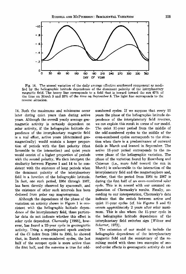
We can easily incorporate the 18% modulation found by Rosenberg and Coleman [1969] for the years 1964-1967 in our model. Figure 14 shows the seasonal variation of the daily averages of the southward component for the two polarities' first, with extra field pointing toward the sun in March and, second, with extra field pointing away from the sun in March. Since the spring peak is due to fields pointing toward the sun and the fall peak is due to fields pointing away from the sun, the first polarity amplifies the spring and fall peaks and the second polarity reduces the peaks. Furthermore, since the variation of the dominant polarity is synchronous with the hellographic latitude of the earth and is therefore maximum on about March and September 5 (an axial effect), it alters the phase of the variation of the southward component.

Examining the U index in Figure 1, we can see an effect similar to that shown in Figure

RUSSELL AND MCPHERRON.' SEMIANNUAL VARIATION 105

-I.0

-.8

-.6

-.4

o {o D•kY OF YE•kR

Fig. 14. The annual variation of the daily average effective southward component as modi- fied by the heliographic latitude dependence of the dominant polarity of the interplanetary magnetic field. The heavy line corresponds to a field that is inward toward the sun 67% of the time on March 5 and 33% of the time on September 5. The light line corresponds to the reverse situation.

14. Both the maximums and minimums occur

later during quiet years than during active years. Although the overall yearly average geomagnetic activity is certainly dependent on solar activity, if the heliographic latitude dependence of the interplanetary magnetic field is a real effect, active years (determined geomagnetically) would contain a larger proportion of periods with the first polarity (that favorable to the interaction) and quiet years would consist of a higher proportion of periods with the second polarity. We then interpret the similarity between Figures I and 14 to be consistent with the existence of long periods when the dominant polarity of the interplanetary field is a function of the heliographic latitude. In fact, one such period, 1964 through 1967, has been directly observed by spacecraft, and the existence of other such intervals has been

deduced from polar cap magnetograms. Although the dependence of the phase of the

variation on activity shown in Figure I is consistent with the heliographic latitude dependence of the interplanetary field, these particular data do not indicate whether this effect is

solar cycle dependent. Chernosky [1966], however, has found a 22-year cycle in geomagnetic activity. Using a superimposed epoch analysis of the Ci index from 1884 to 1963, he showed that, in Zurich even-numbered cycles, the last half of the sunspot cycle is more active than the first half, and the converse is true for odd-

numbered cycles. If we suppose that every 11 years the phase of the heliographic latitude dependence of the interplanetary field reverses, we can explain this result in terms of our model. The quiet 11-year period from the middle of the odd-numbered cycles to the middle of the even-numbered cycles corresponds to the situation when there is a predominance of outward fields in March and inward in September. The active 11-year period corresponds to the reverse phase of the heliographie variation. The phase of the variation found by Rosenberg and Coleman (i.e., more field toward the sun in March) is unfavorable to the interaction of the interplanetary field and the magnetosphere and, further, that the period from 1964 to 1967 is during the first half of an even-numbered solar eyre. This is in accord with our assumed explanation of Chernosky's results. Finally, according to our interpretation, Chernosky's data indicate that the switch between active and

quiet l 1-year cycles (ef. his Figures 5 and 6) occurs approximately 2 years after solar maximum. This is also where the l 1-year cycle in the heliographie latitude dependence of the interplanetary field switches sign [Wilcox and Scherrer, 1972].

The extension of our model to include the

heliographie dependence of the interplanetary magnetic field and the consistency of the re- suiting model with these two examples of second-order effects in geomagnetic activity do not

106 RUSSELL ^ND McPHERRON: SE•VtI^NNU^L V^RI^?IO•

prove that our simple model is correct. They do indicate, however, that this mechanism can account for several subtle features of the semi-

annual variation, and thus these observations provide a successful test of the mechanism.

I)ISCUSSION

Since the southward component of the interplanetary field as measured in solar magnetospheric coordinates is modulated by the tilt of the earth's rotation axis relative to the ecliptic pole and the tilt of the dipole axis to this rotation axis, as well as by the tilt of the sun's axis of rotation to the ecliptic pole, our model for the semiannual variation of geomagnetic activity is both an equinoctial and an axial hypothesis. The inclusion of the heliographic latitude dependence of the dominant polarity of the interplanetary field is a further axial effect. However, these axial dependences of the model differ from previous axial hypotheses in which latitudinal variations in solar streams

were postulated [cf. Cottie, 1912]. Latitudinal structure does, in fact, exist in the solar wind [Hundhausen et al., 1971], and we cannot rule out the possibility that this latitudinal structure does play some role in the semiannual variation of geomagnetic activity. However, the separation of geomagnetic activity into two annual variations with different phases, upon ordering by the polarity of the interplanetary magnetic field, indicates that this is a minor role. We further note that, though geomagnetic activity closely follows solar activity, Hund- hausen et al. [1971] and Gosling et al. [1971] have shown that there has been very little variation in the average solar wind velocity or number density during the present solar cycle.

Coleman and Smith [1966] have shown that an amplitude modulation of geomagnetic activity with a period of 1 year exists. None of the models we have examined has this modulation.

Such an annual modulation could be caused by • north-south asymrnetry in the latitudinal variation of the interplanetary magnetic field or of the solar wind parameters. However, it is improbable that such an asymmetry would persist for periods longer than one solar cycle.

Finally, we note that correlations of the polarity of the interplanetary magnetic field with magnetospheric phenomena obtained from a

single earth-orbiting spacecraft should be viewed with some caution. Because of the motion of

the earth about the sun, earth-orbiting spacecraft that probe the interplanetary rnedium are in the solar wind during the same season each

year. As we have shown, interplanet. ary magnetic fields toward the sun on the average have a southward component in solar magnetospheric coordinates in the spring, but outward fields on the average have a southward component in the fall. Therefore, a .process that depends on the southward component may correlate with the polarity of the interplanetary field if the correlation is studied during one season. Thus we interpret the observation of $chatten and Wilcox [1967], who used Imp 3 data in the solar wind from June 1965 through January 1966, that outward sectors were associated with greater geomagnetic activity than inward sectors, as merely a reflection of the average southward component of outward sectors during the fall.

A similar effect can occur when measure-

ments in the magnetotail are correlated with the polarity of the interplanetary magnetic field. For example, Hruska [1971] has shown that neutral sheet crossings were on the average displaced northward of the magnetospheric equator when the interplanetary field was outward from the sun. However, since these observations were made on Imp 3, which was in the magnetotail during April and May, outward fields would have on the average a northward solar magnetospheric component. Thus, it is possible that the displacement of the neutral sheet is related instead to the north-south com-

ponent of the interplanetary field rather than the radial component.

CONCLUSIONS

The semiannual variation in geomagnetic activity as measured by counting storms of intensity above a given threshold is manifested in the fact that twice as many storms occur on the average during the equinoctial months as during the solstitial months. If this is caused by a mechanism that modulates the energy extracted from incipient storm-producing plasma in the solar wind throughout the year, this variation in storm counts can be caused by a 40% increase in the average energy input dur-

t{USSELL AND MCPHERRON: SEMIANNUAL VARIATION 107

ing a storm at the equinoxes relative to the average energy deposited at the solstices.

By examining four models of the interaction, three involving the southward component and one involving the Kelvin-Helmholtz instability, we have found that only two models produce a semiannual variation in phase with that observed. The model assuming simple merging in solar magnetospheric coordinates and the model assuming that the interaction is ordered in solar magnetic coordinates both failed to produce the observed phase of semiannual variation.

A model, in which the interaction, ordered in solar magnetospheric coordinates, is zero for northward components of the interplanetary field while the interaction is proportional to magnitude of the southward components predicts the correct phase and provides a yearly variation in •he strength of the interaction sufficient to cause the observed effect. Further-

more, the prediction of this model, that the semiannual variation of geomagnetic activity can be split into two annual variations, one peaking in spring and one in fall, if geomagnetic activity is ordered according to the polarity of the interplanetary field, is confirmed. Further evidence that the interplanetary field controls the semiannual variation comes from

the variable phase of the semiannual variation and the existence of a 22-year cycle in geomagnetic activity. The 22-year variation is in phase with the 22-year variation of the interplanetary magnetic field as found from polar cap magnetograms over a 45-year period.

The model that assumes that the Kelvin-

Helmholtz instability causes the drag on the magnetosphere, though not quantitative, also predicts the observed phase of the semiannual variation. This model does differ significantly in its prediction of the diurnal variation from the prediction of our above model. In this model, the predicted interaction at the magnetopause is in phase with the observed activity at the ground, whereas in our solar magnetospheric model the observed activity lags the interaction by 6 hours. Either phase lag is con- ceptually possible, depending on the details of the storage of energy on the tail. Further, since the phase of the diurnal variation is dependent on the exact details of the model, the predicted

phase will change as the model is refined. Thus, we do not consider that the differences in the

predicted diurnal variations permit a decisive test of the two mechanisms.

Although the model will have to be refined as we achieve a better understanding of the laws governing the rate of energy transfer from the solar wind to the magnetosphere, the fact that we can construct a model, using the interplanetary field orientation as the causative agent, that (1) is consistent with our present knowledge of this interaction, (2) reproduces the semiannual variation, and (3) explains even subtle features of this variation indicates that

we have isolated the mechanism causing the semiannual variation of geomagnetic activity. This mechanism is the varying probability throughout the year of a southward component of the interplanetary magnetic field as seen by the magnetosphere. This arises from the changing orientation between the solar equatorial coordinate system, in which the interplanetary field is ordered, and the solar magnetospheric coordinate system, in which the interaction with the interplanetary field is ordered.

Acknowledgments. We wish to acknowledge several fruitful discussions of the merging of the interplanetary and magnetospheric fields with G. Atkinson and D. J. Southwood and of the domi-

nant polarity of the interplanetary magnetic field with R. L. Rosenberg. The Dst data were pro- vided by W. E. Valente of the National Space Science Data Center.

This study was supported by NASA grant NGR 054)07-305.

The Editor thanks J. Hirshberg and J. M. Wilcox for their assistance in evaluating this paper.

REFERENCES

Arnoldy, R. L., Signature in the interplanetary medium for substorms, J. Geophys. Res., 76(22), 5189-5201, 1971.

Boller, B. R., and H. L. Stolov, Kelvin-Helmholtz instability and the semiannual variation of geomagnetic activity, J. Geophys. Res., 75(3!), 6073-7084, 1970.

Burch, J. L., Effect of interplanetary magnetic field azimuth on auroral zone and polar cap magnetic activity, submitted to J. Geophys. Res., 1972.

Chapman, S., and J. Bartels, Geomagnetism, chap. 11, Oxford University Press, New York, 1940.

108 RUSSELL AND McP•EaaON: SEMIANNUAL VARIATION

Chernosky, E. J., Double sun'spot-cycle variation in terrestrial magnetic activity, 1884-1963, J. Geophys. Res., 71(3), 965-974, 1966.

Coleman, P. J., Jr., Variations in the interplanetary magnetic field: Mariner 2, 1, Observed properties, J. Geophys. Res., 7(23), 5509-5531, 1966.

Coleman, P. J., Jr., and E. J. Smith, An interpretation of the subsidiary peaks at periods near 27 days in the power spectra of Ci and Kp, J. Geophys. Res., 71(19), 4685-4686, 1966.

Cartie, A. L., Sunspots and terrestrial magnetic phenomena, 1898-1911, Man. Notic. Roy. As- tron.. Sac., 73, 52-60, 1912.

Foster, J. C., D. H. Fairfield, K. W. Ogilvie, and T. J. Rosenberg, Relationship of interplanetary parameters and occurrence of magnetospheric substorms, J. Geophys. Res., 76(28), 6971-6975, 1971.

Fraser-Smith, A. C., The spectrum of the geomagnetic activity index Ap, J. Geophys. Res., 77(22), 4209, 1972.

Gosling, J. T., R. T. Hansen, and S. J. Bame, Solar wind speed distributions: 1962-1970, J. Geophys. Res., 76(7), 1811-1815, 1971.

Hirshberg, J., and D. S. Colburn, Interplanetary field and geomagnetic variations: A .unified view, Planet. Space Sci., 17, 1183-1206, 1969.

Hruska, A., Electric current system in the un- disturbed magnetospheric tail, Radio Sci., 6(2), 295-298, 1971.

Hundhausen, A. J., S. J. Bame, and M.D. Mont- gomery, Variations of solar-wind plasma properties: Vela observations of a possible heliographic latitude-dependence, J. Geophys. Res., 76(22), 5145-5154, 1971.

Mcintosh, D. H., On the annual variation of magnetic disturbance, Phil. Trans. Roy. Sac. London, Ser. A, 251, 525-552, 1959.

Petschek, H. W., Magnetic field annihilation, in AAS-NASA Symposium on the Physics of Solar Flares, NASA Spec. Publ. 50, 425, 1964.

Piddington, J. H., Theories of the geomagnetic storm main phase, Planet. Space Sci., 11, 1277, 1963.

Rosenberg, R. L., Unified theory of the inter- planetaw magnetic field, Solar Phys., 15(1), 72-78, 1970.

Rosenberg, R. L., and P. J. Coleman, Jr., Helio- graphic latitude dependence' of the dominant polarity of the interplanetary magnetic field, J. Geophys. Res., 74(24), 5611-5622, 1969.

Russell, C. T., Geophysical coordinate transforma- tions, Cosmic Electrodynamics, 2(2), 184-196, 1971.

Schatten, K. H., and J. M. Wilcox, Response of the geomagnetic activity index Kp to the interplanetary magnetic field, J. Geophys. Res., 72(21), 5185-5191, 1967.

Sckopke, N., A general relation between the energy of trapped particles and the disturbance field near the earth, J. Geophys. Res., 71(13), 3125, 1966.

Snyder, C. W., M. Neugebauer, and U. R. Rao, The solar wind velocity and its correlation with cosmic ray variations and with solar and geomagnetic activity, J. Geophys. Res., 68(24), 6361-6370, 1963.

Wilcox, J. M., Statistical significance of the proposed heliographic latitude dependence of the dominant polarity of the interplanetary magnetic field, J. Geophys. Res., 75(13), 2587-2590, 1970.

Wilcox, J. M., and D. S. Colburn, Interplanetary sector structure near the maximum of the sun-

spot cycle, J. Geophys. Res., 75(31), 6366-6370, 1970.

Wilcox, J. M., and P. H. Scherrer, Annual and solar-magnetic-cycle variations in the interplanetary magnetic field, 1926-1971, J. Geophys. Res., 77 (28), 5385-5388, 1972.

Wilcox, J. M., K. H. Schatten, and N. F. Ness, Influence of interplanetary magnetic field and plasma on geomagnetic activity during quiet- sun conditions, J. Geophys. Res., 72(1), 19-26, 1967.

(Received January 17, 1972; accepted September 29, 1972.)

Documents

Semiannual Variation of Geomagnetic Activity · 94 RUSSELL AND MCP•ERRON: SEMIANNUAL VARIATION Although geomagnetic indices such as the U index of 'Figure 1, Ci, Kp, or Ap provide