Semigroups and Evolution Equations: Functional … · Semigroups and evolution equations: Functional calculus, regularity and kernel estimates 3 Introduction The theory of one-parameter

CHAPTER 1

Semigroups and Evolution Equations: FunctionalCalculus, Regularity and Kernel Estimates

Wolfgang ArendtAbteilung Angewandte Analysis, Universität Ulm, 89069 Ulm, Germany,

E-mail: [email protected]

ContentsIntroduction . . . . . . . . . . . . . . . . . . . . . . . . . . . . . . . . . . . . . . . . . . . . . . . . . . . . . 31. Semigroups . . . . . . . . . . . . . . . . . . . . . . . . . . . . . . . . . . . . . . . . . . . . . . . . . . . 4

1.1. The algebraic approach . . . . . . . . . . . . . . . . . . . . . . . . . . . . . . . . . . . . . . . . . 41.2. The Cauchy problem . . . . . . . . . . . . . . . . . . . . . . . . . . . . . . . . . . . . . . . . . . 51.3. Semigroups and Laplace transforms . . . . . . . . . . . . . . . . . . . . . . . . . . . . . . . . . . 51.4. More general C0-semigroups . . . . . . . . . . . . . . . . . . . . . . . . . . . . . . . . . . . . . . 61.5. The inhomogeneous Cauchy problem . . . . . . . . . . . . . . . . . . . . . . . . . . . . . . . . . 6

2. Holomorphic semigroups . . . . . . . . . . . . . . . . . . . . . . . . . . . . . . . . . . . . . . . . . . . . 72.1. Characterization of bounded holomorphic semigroups . . . . . . . . . . . . . . . . . . . . . . . . 72.2. Characterization of holomorphic semigroups . . . . . . . . . . . . . . . . . . . . . . . . . . . . . 72.3. Boundary groups . . . . . . . . . . . . . . . . . . . . . . . . . . . . . . . . . . . . . . . . . . . . . 72.4. The Gaussian semigroup . . . . . . . . . . . . . . . . . . . . . . . . . . . . . . . . . . . . . . . . 82.5. The Dirichlet Laplacian . . . . . . . . . . . . . . . . . . . . . . . . . . . . . . . . . . . . . . . . . 82.6. The Neumann Laplacian on C(�Ω) . . . . . . . . . . . . . . . . . . . . . . . . . . . . . . . . . . . 102.7. Wentzell boundary conditions . . . . . . . . . . . . . . . . . . . . . . . . . . . . . . . . . . . . . . 112.8. Dynamic boundary conditions . . . . . . . . . . . . . . . . . . . . . . . . . . . . . . . . . . . . . 11

3. Asymptotics . . . . . . . . . . . . . . . . . . . . . . . . . . . . . . . . . . . . . . . . . . . . . . . . . . . 123.1. Exponential stability . . . . . . . . . . . . . . . . . . . . . . . . . . . . . . . . . . . . . . . . . . . 123.2. Ergodic semigroups . . . . . . . . . . . . . . . . . . . . . . . . . . . . . . . . . . . . . . . . . . . 143.3. Convergence and asymptotically almost periodicity . . . . . . . . . . . . . . . . . . . . . . . . . . 153.4. Positive semigroups . . . . . . . . . . . . . . . . . . . . . . . . . . . . . . . . . . . . . . . . . . . 163.5. Positive irreducible semigroup . . . . . . . . . . . . . . . . . . . . . . . . . . . . . . . . . . . . . 17

4. Functional calculus . . . . . . . . . . . . . . . . . . . . . . . . . . . . . . . . . . . . . . . . . . . . . . . 184.1. Sectorial operators . . . . . . . . . . . . . . . . . . . . . . . . . . . . . . . . . . . . . . . . . . . . 184.2. The sum of commuting operators . . . . . . . . . . . . . . . . . . . . . . . . . . . . . . . . . . . . 194.3. The elementary functional calculus . . . . . . . . . . . . . . . . . . . . . . . . . . . . . . . . . . . 204.4. Fractional powers and BIP . . . . . . . . . . . . . . . . . . . . . . . . . . . . . . . . . . . . . . . 234.5. Bounded H∞-calculus for sectorial operators . . . . . . . . . . . . . . . . . . . . . . . . . . . . . 28

HANDBOOK OF DIFFERENTIAL EQUATIONSEvolutionary Equations, volume 1Edited by C.M. Dafermos and E. Feireisl© 2004 Elsevier B.V. All rights reserved

1

2 W. Arendt

4.6. Perturbation . . . . . . . . . . . . . . . . . . . . . . . . . . . . . . . . . . . . . . . . . . . . . . . 334.7. Groups and positive contraction semigroups . . . . . . . . . . . . . . . . . . . . . . . . . . . . . . 33

5. Form methods and functional calculus . . . . . . . . . . . . . . . . . . . . . . . . . . . . . . . . . . . . 355.1. Bounded H∞-calculus on Hilbert space . . . . . . . . . . . . . . . . . . . . . . . . . . . . . . . . 355.2. m-accretive operators on Hilbert space . . . . . . . . . . . . . . . . . . . . . . . . . . . . . . . . . 365.3. Form methods . . . . . . . . . . . . . . . . . . . . . . . . . . . . . . . . . . . . . . . . . . . . . . 385.4. Form sums and Trotter’s product formula . . . . . . . . . . . . . . . . . . . . . . . . . . . . . . . 415.5. The square root property . . . . . . . . . . . . . . . . . . . . . . . . . . . . . . . . . . . . . . . . 445.6. Groups and cosine functions . . . . . . . . . . . . . . . . . . . . . . . . . . . . . . . . . . . . . . 45

6. Fourier multipliers and maximal regularity . . . . . . . . . . . . . . . . . . . . . . . . . . . . . . . . . . 496.1. Vector-valued Fourier series and periodic multipliers . . . . . . . . . . . . . . . . . . . . . . . . . 496.2. Maximal regularity via periodic multipliers . . . . . . . . . . . . . . . . . . . . . . . . . . . . . . 53

7. Gaussian estimates and ultracontractivity . . . . . . . . . . . . . . . . . . . . . . . . . . . . . . . . . . . 597.1. The Beurling–Deny criteria . . . . . . . . . . . . . . . . . . . . . . . . . . . . . . . . . . . . . . . 597.2. Extrapolating semigroups . . . . . . . . . . . . . . . . . . . . . . . . . . . . . . . . . . . . . . . . 607.3. Ultracontractivity, kernels and Sobolev embedding . . . . . . . . . . . . . . . . . . . . . . . . . . 647.4. Gaussian estimates . . . . . . . . . . . . . . . . . . . . . . . . . . . . . . . . . . . . . . . . . . . . 69

8. Elliptic operators . . . . . . . . . . . . . . . . . . . . . . . . . . . . . . . . . . . . . . . . . . . . . . . . 728.1. Boundary conditions . . . . . . . . . . . . . . . . . . . . . . . . . . . . . . . . . . . . . . . . . . . 738.2. Positivity and irreducibility . . . . . . . . . . . . . . . . . . . . . . . . . . . . . . . . . . . . . . . 738.3. Submarkov property: Dirichlet boundary conditions . . . . . . . . . . . . . . . . . . . . . . . . . 748.4. Quasicontractivity in Lp . . . . . . . . . . . . . . . . . . . . . . . . . . . . . . . . . . . . . . . . 748.5. Gaussian estimates: real coefficients . . . . . . . . . . . . . . . . . . . . . . . . . . . . . . . . . . 748.6. Complex second-order coefficients . . . . . . . . . . . . . . . . . . . . . . . . . . . . . . . . . . . 758.7. Further comments on Gaussian estimates . . . . . . . . . . . . . . . . . . . . . . . . . . . . . . . 758.8. The square root property . . . . . . . . . . . . . . . . . . . . . . . . . . . . . . . . . . . . . . . . 768.9. The hyperbolic equation . . . . . . . . . . . . . . . . . . . . . . . . . . . . . . . . . . . . . . . . . 76

8.10. Nondivergence form . . . . . . . . . . . . . . . . . . . . . . . . . . . . . . . . . . . . . . . . . . . 778.11. Elliptic operators with Banach space-valued coefficients . . . . . . . . . . . . . . . . . . . . . . . 77

Acknowledgments . . . . . . . . . . . . . . . . . . . . . . . . . . . . . . . . . . . . . . . . . . . . . . . . . 78References . . . . . . . . . . . . . . . . . . . . . . . . . . . . . . . . . . . . . . . . . . . . . . . . . . . . . 78

Monographs . . . . . . . . . . . . . . . . . . . . . . . . . . . . . . . . . . . . . . . . . . . . . . . . . . . 78Research Articles . . . . . . . . . . . . . . . . . . . . . . . . . . . . . . . . . . . . . . . . . . . . . . . . 79

AbstractThis is a survey on recent developments of the theory of one-parameter semigroups and

evolution equations with special emphasis on functional calculus and kernel estimates. Alsoother topics as asymptotic behavior for large time and holomorphic semigroups are discussed.As main application we consider elliptic operators with various boundary conditions.

Semigroups and evolution equations: Functional calculus, regularity and kernel estimates 3

Introduction

The theory of one-parameter semigroups provides a framework and tools to solve evolu-tionary problems. It is impossible to give an account of this rich and most active field.In this chapter we rather try to present a survey on a particular subject, namely functionalcalculus, maximal regularity and kernel estimates which, in our eyes, has seen a mostspectacular development, and which, so far, is not presented in book form. We commenton these three subjects:

1. Functional calculus (Section 4). If A is a self-adjoint operator, one can define f (A)

for all bounded complex-valued measurable functions defined on the spectrum of A. It wasMcIntosh who initiated and developed a theory of functional calculus for a less restrictedlarge class of operators, namely sectorial operators; i.e., operators whose spectrum is in-cluded in a sector and whose resolvent satisfies a certain estimate. Negative generatorsof bounded holomorphic semigroups are sectorial operators and are our main subject ofinvestigation. And indeed, for these operators f (A) can be defined for a large class ofholomorphic functions defined on a sector containing the spectrum. Taking f (z) = e−tz

leads to the semigroup e−tA, the function f (z) = zα to the fractional power of such anoperator A. One important reason to study functional calculus is the Dore–Venni theorem.In its hypotheses functional calculus plays a role; the conclusion is the invertibility of thesum of two operators A and B . Thus, the Dore–Venni theorem asserts that the equation

Ax +Bx = y

has a unique solution x ∈D(A)∩D(B). To say that the solution is at the same time in bothdomains can be rephrased by saying that the solution has “maximal regularity”, a crucialproperty in many circumstances.

2. Form methods (Section 5). On Hilbert space the functional calculus behaves particu-larly well as we show in Sections 4 and 5. Most interesting is the close connection withform methods. Basically, the following is true: an operator is associated with a form ifand only if it has a bounded H∞-calculus. Form methods, based on the fundamental Lax–Milgram lemma, allow a most efficient treatment of elliptic and parabolic problems as weshow later.

3. Maximal regularity and Fourier transform (Section 6). The following particular prob-lem of maximal regularity is important for solving nonlinear equations: The genera-tor A of a semigroup T is said to have property (MR) if T ∗ f ∈ W 1,2((0,1);X) forall f ∈ L2((0,1);X). On Hilbert spaces every generator of a holomorphic semigrouphas (MR); but a striking result of Kalton–Lancien asserts that this fact characterizesHilbert spaces (among a large class of Banach spaces). On the other hand, in recentyears it has been understood which role “unconditional properties” play for operator-valued Fourier transform and Cauchy problems. So one may characterize property (MR)

by R-boundedness, a property defining “unconditional boundedness” of sets of operators.

4 W. Arendt

4. Kernel estimates (Section 7). Gaussian estimates for the kernels of parabolic equationshave been investigated for many years. It is most interesting in its own right that the solu-tions of a parabolic equation with measurable coefficients are very close to the Gaussiansemigroup. But Gaussian estimates have also striking consequences for the underlyingsemigroup. For example, we show that they do imply boundedness of the H∞-calculus.

5. Elliptic operators (Section 8). The theory presented here can be applied to elliptic op-erators with measurable coefficients to which Section 8 is devoted. We will explain Kato’ssquare root problem, the most difficult question of coincidence of form domain and thedomain of the square root, which has been solved recently by Auscher, Hofmann, Lacey,McIntosh and Tchamitchian.

We start the chapter by putting together some basic properties of semigroups whichare particularly useful in the sequel. Special attention is given to holomorphic semigroups(Section 2) and to the theory of asymptotic behavior (Section 3). As prototype examplein this account serve the Laplacian with Dirichlet and Neumann boundary conditions:On spaces of continuous functions this operator will be considered in Section 2, later itsLp-properties are established. Concerning the results on asymptotic behavior we concen-trate on those which can be applied to parabolic equations in Section 8.

Most of the results are presented without proof, referring to the literature. Frequently,only particular cases which are easy to formulate are presented; and in a few cases we giveproofs. Some of them are new, not very well known or particularly elegant. The articlepresents a special choice, guided by personal taste, even in this narrow subject. We hopethat the numerous references allow reader to go beyond that choice and that the list ofmonographs at the end helps them to view the subject in a broader context.

1. Semigroups

In this introductory section we present semigroups from three different points of view.We mention few properties but refer to the various text books concerning the theory.

1.1. The algebraic approach

Let X be a complex Banach space, let C(R+,X) be the space of all continuous functionsdefined on R+ := [0,∞) with values in X. A C0-semigroup is a mapping T : R+→ L(X)

such that(a) T (·)x ∈C(R+,X) for all x ∈X;(b) T (0)= I ;(c) T (s + t)= T (s)T (t), s, t ∈R+.

Given a C0-semigroup T on X, one defines the generator A of T as an unbounded operatoron X by

Ax = limt↓0

T (t)x − x

t


with domain D(A) := {x ∈X: limt↓0T (t)x−x

texists}. Then D(A) is dense in X and A is

closed and linear. In other words, A is the derivative of T in 0 (in the strong sense) and forthis reason one also calls A the infinitesimal generator of T .

The second approach involves the Cauchy problem.

1.2. The Cauchy problem

Let A be a closed linear operator on X. Let J ⊂ R be an interval. A mild solution of thedifferential equation

u(t)=Au(t), t ∈ J, (1.1)

is a function u(t) ∈C(J,X) such that∫ t

su(r)dr ∈D(A) for all s, t ∈ J and A

∫ t

su(r)dr =

u(t) − u(s). A classical solution is a function u ∈ C1(J,X) such that u(t) ∈ D(A) andu(t)=Au(t) for all t ∈ J . Since A is closed, a mild solution u is a classical solution if andonly if u ∈ C1(J,X).

THEOREM [[ABHN01], 3.1.12]. Let J = [0,∞). The following assertions are equivalent:(i) A generates a C0-semigroup T ;

(ii) for all x ∈X, there exists a unique mild solution u of (1.1) satisfying u(0)= x .In that case u(t)= T (t)x , t � 0.

The theorem implies in particular that the generator A determines uniquely the semi-group. Here is the third approach.

1.3. Semigroups and Laplace transforms

Let T be a C0-semigroup with generator A. Then the growth bound

ω(T ) := inf{ω ∈R: ∃M such that

∥∥T (t)∥∥� Meωt for all t � 0

}satisfies −∞� ω(T ) <∞, and if λ ∈C, Reλ > ω(T ), then λ is in the resolvent set ρ(A)

of A and

R(λ,A)x =∫ ∞

0e−λtT (t)x dt := lim

τ→∞

∫ τ

0e−λtT (t)x dt

for all x ∈X, where R(λ,A)= (λ−A)−1.

THEOREM [[ABHN01], Theorem 3.1.7, p. 113]. Let T : R+→L(X) be strongly continu-ous. Let A be an operator on X, λ0 ∈R such that (λ0,∞)⊂ ρ(A) and

R(λ,A)x =∫ ∞

0e−λtT (t)x dt, λ > λ0,

6 W. Arendt

for all x ∈X. Then T is a C0-semigroup and A its generator.

Thus generators of C0-semigroups are precisely those operators whose resolvent is aLaplace transform. Laplace transform techniques play an important role in semigroup the-ory (see [[ABHN01]] for a systematic theory).

1.4. More general C0-semigroups

In order to talk about Dirichlet boundary conditions we need more general semigroups (cf.Section 2.5). A strongly continuous function T : (0,∞)→ L(X) is called a (nondegeneratelocally bounded ) semigroup if

(a) T (t)T (s)= T (t + s), t, s > 0;(b) sup0<t�1 ‖T (t)‖<∞;(c) T (t)x = 0 for all t > 0 implies x = 0.

As a consequence ω(T ) <∞ and there exists a unique operator A such that (ω(T ),∞)⊂ρ(A) and R(λ,A)x = ∫∞0 e−λtT (t)x dt for all x ∈X and λ > ω(T ). We call A the gener-ator of T (see [[ABHN01], 3.2]). Then T is a C0-semigroup if and only if D(A) =X. IfX is reflexive, then this is automatically true.

1.5. The inhomogeneous Cauchy problem

If A generates a C0-semigroup T , then also the inhomogeneous Cauchy problem{u(t)=Au(t)+ f (t), t ∈ [0, τ ],u(0)= x

(1.2)

is well posed. More precisely, let x ∈ X, f ∈ L1((0, τ );X). A mild solution of (1.2) is acontinuous function u : [0, τ ]→X such that

∫ t

0 u(s)ds ∈D(A) and

u(t)− x =A

∫ t

0u(s)ds +

∫ t

0f (s)ds

for all t ∈ [0, τ ]. Define T ∗ f by T ∗ f (t)= ∫ t

0 T (t − s)f (s)ds.

PROPOSITION. The function u given by u(t)= T (t)x + T ∗ f (t) is the unique mild solu-tion of (1.2).

1.5.1. Classical solutions. Thus, in the particular case where x = 0, the mild solutionof (1.2) is u = T ∗ f . It is very rare that this u is a classical solution for all f . Let T bea C0-semigroup on X with generator A.

THEOREM (Baillon; see [EG92]). Assume that X is reflexive or X = L1 (or more generallythat c0 �⊂X). If for all f ∈ C([0, τ ];X) one has T ∗f ∈ C1([0, τ ],X), then A is bounded.


In Section 5 we will devote much attention to the question when

T ∗ f ∈W 1,p((0, τ );X) for all f ∈ Lp((0, τ );X).

2. Holomorphic semigroups

A semigroup T : (0,∞)→ X (in the sense of Section 1.4) is called holomorphic if thereexists θ ∈ (0,π/2] such that T has a holomorphic extension T :Σθ → L(X) which isbounded on {z ∈ Σθ : |z| � 1}. In that case, this holomorphic extension is unique andsatisfies T (z1 + z2)= T (z1)T (z2) for all z1, z2 ∈Σθ . If T is a C0-semigroup, then

limz→0z∈Σθ

T (z)x = x

for all x ∈X, and we call T a holomorphic C0-semigroup. If the extension T is boundedon Σθ , we call T a bounded holomorphic semigroup. Thus, for this property, it does notsuffice that T is bounded on [0,∞). Take for example, T (t)= eit on X =C.

2.1. Characterization of bounded holomorphic semigroups

Let A be an operator on X. The following assertions are equivalent:(i) A generates a bounded holomorphic semigroup T ;

(ii) one has λ ∈ ρ(A) whenever Reλ > 0 and supReλ>0 ‖λR(λ,A)‖<∞;(iii) there exists α ∈ (0,π/2) such that e±iαA generates a bounded semigroup.

In that case (T (e±iαt))t�0 is the semigroup generated by e±iαA. Moreover, T is aC0-semigroup if and only if D(A) is dense. This is automatic whenever X is reflexive.

2.2. Characterization of holomorphic semigroups

An operator A generates a holomorphic semigroup T if and only if there exists ω such thatA−ω generates a bounded holomorphic semigroup S. In that case T (t)= eωtS(t), t � 0.

2.3. Boundary groups

Let A be the generator of a C0-semigroup T having a holomorphic extension to thehalf-plane C+ = {λ ∈ C: Reλ > 0}. Then iA generates a C0-group U if and only ifsupRez>0,|z|�1 ‖T (z)‖<∞.

In that case we call U the boundary group of T and write U(s)=: T (is), s ∈R.

8 W. Arendt

2.4. The Gaussian semigroup

Consider the Gaussian semigroup G defined on L1 +L∞ := L1(Rn)+L∞(Rn) by

(G(z)f

)(x)= (4πz)−n/2

∫Rn

f (y)e−(x−y)2/4z dy (2.1)

for all x ∈ Rn, f ∈ L1 + L∞, Re z > 0. Then G is a holomorphic semigroup which isbounded on Σθ for each 0 < θ < π/2. The generator �1+∞ of G is given by

D(�1+∞)= {f ∈ L1 +L∞: �f ∈ L1 +L∞},

�1+∞f =�f in D(Rn)′.

Let E be one of the spaces Lp(Rn), 1 � p � ∞, Cb(Rn) = {f ∈ L∞(Rn): f iscontinuous};

BUC(Rn) := {f ∈ Cb(Rn

): f is uniformly continuous

},

C0(Rn) := {f ∈Cb(Rn

): lim|x|→∞

∣∣f (x)∣∣= 0

},

which are all subspaces of L1 + L∞. Then the restriction G(t)|E

defines a holomorphicsemigroup GE on E which is bounded on Σθ for each θ ∈ (0,π/2). Its generator is �E

given by

D(�E)= {f ∈E: �f ∈E},�Ef =�f in D

(Rn)′.

On E = Lp(Rn), 1 � p <∞, BUC(Rn) and C0(Rn) the semigroup GE is a C0-semi-

group.

2.5. The Dirichlet Laplacian

In this section we introduce the Laplacian with Dirichlet boundary conditions on thespace C(�Ω). It is a most basic example and we show in an elementary way that it gen-erates a holomorphic semigroup.

Let Ω ⊂ Rn be open and bounded. We assume that Ω is Dirichlet regular; i.e., for allϕ ∈C(∂Ω) there exists a solution of

D(ϕ)

{h ∈ C

(�Ω ), h|∂Ω = ϕ,

�h= 0 in D(Ω)′.

Such a solution is unique and automatically in C∞(Ω). If Ω has Lipschitz boundary, thenΩ is Dirichlet regular, but much milder geometric assumptions suffice (see, e.g., [[DL88],


Chapter II]). We consider the operator A defined on C(�Ω) by

D(A)= {u ∈ C0(Ω): �u ∈C(�Ω )},

Au=�u in D(Ω)′,

where C0(Ω) := {u ∈ C(�Ω): u|∂Ω = 0} and D(Ω)′ denotes the space of all distributions.We call A the Dirichlet Laplacian on C(�Ω).

THEOREM. The operator A generates a bounded holomorphic semigroup T on C(�Ω).

For the proof we need the following form of the maximum principle.

MAXIMUM PRINCIPLE. Let v ∈C(�Ω) such that λv−�v = 0 in D(Ω)′, where Reλ > 0.Then

supx∈∂Ω

∣∣v(x)∣∣= supx∈�Ω

∣∣v(x)∣∣.PROOF. Suppose that ‖v‖L∞(Ω) > supx∈∂Ω |v(x)|. Let K := {x ∈Ω : |v(x)| = ‖v‖∞} andvε = ρε ∗ v, where ρε is a mollifier. Then vε → v, �vε = ρε ∗�v → �v uniformly oncompact subsets of Ω as ε ↓ 0. Let Ω1 ⊂Ω be relatively compact such that K ⊂Ω1 and�Ω1 ⊂Ω . Then, for small ε > 0, there exists xε ∈Ω1 such that |vε(xε)| = supx∈Ω1

|vε(x)|.Then

Re[�vε(xε)vε(xε)

]� 0. (2.2)

In fact, consider the function f (y)= Revε(y)vε(xε). Then f has a local maximum in xε .Hence �f (xε) � 0. Let xεn → x0. Since vεn → v uniformly on Ω1, it follows that x0 ∈K .From (2.2) we deduce that Re[v(x0)�v(x0)]� 0. Hence,

Reλ∣∣v(x0)

∣∣2 � Reλ∣∣v(x0)

∣∣2 −Re[v(x0)�v(x0)

]= Re

[v(x0)

(λv(x0)−�v(x0)

)]= 0.

Since x0 ∈K , it follows that v = 0, contradicting the assumption. �

PROOF OF THE THEOREM. (a) Similarly as the Maximum principle above, one shows thatA is dissipative.

(b) We show that 0 ∈ ρ(A). Let f ∈ C(�Ω). Denote by f the extension of f to Rn

by 0 and let v =E ∗ f , where E is the Newtonian potential. Then v ∈ C(Rn) and �v = f

in D(Ω)′. Let ϕ = v|∂Ω and consider the solution h of the Dirichlet problem D(ϕ). Thenu= v − h ∈D(A) and Au= f . We have shown that A is surjective. Since the solution ofD(0) is unique, the operator A is injective. Since A is closed, it follows that 0 ∈ ρ(A).

(c) It follows from (a) and (b) that A is m-dissipative. In particular, λ ∈ ρ(A) wheneverReλ > 0.

10 W. Arendt

(d) Denote by �0 the Laplacian on C0(Rn) which generates a bounded holomorphic

semigroup by 2.4. Thus there exists M � 0 such that∥∥λR(λ,�0)∥∥� M if Reλ > 0.

We show that ‖λR(λ,A)‖ � 2M if Reλ > 0 which proves the Theorem. In fact, letReλ > 0, f ∈ C(�Ω), g = R(λ,A)f . Let g =R(λ,�∞)f . Then v = g− g ∈ C(�Ω). More-over, v|∂Ω =−g|∂Ω and λv −�v = 0 in D(Ω)′. By the Maximum principle, one has

supx∈�Ω

∣∣v(x)∣∣ = supx∈∂Ω

∣∣v(x)∣∣= supx∈∂Ω

∣∣g(x)∣∣� M

|λ|∥∥f ∥∥

L∞(Rn)= M

|λ|‖f ‖L∞(Ω).

Consequently,

‖g‖L∞(Ω) � ‖v‖L∞(Ω) +∥∥g∥∥

L∞(Ω)

� 2M

|λ| ‖f ‖L∞(Ω). �

FURTHER PROPERTIES. One has ω(T ) <∞ and T (t) is positive and compact for allt > 0. The restriction T0 of T to C0(Ω) is a C0-semigroup.

REFERENCE. The elegant elementary argument above is due to Lumer and Paquet [LP79],where it is given for more general elliptic operators. See also [[ABHN01], Chapter 6] fora different presentation, and [LS99] for more general results.

2.6. The Neumann Laplacian on C(�Ω)

Let Ω ⊂ Rn be open. There is a natural realization �NΩ of the Laplacian on L2(Ω) with

Neumann boundary conditions. The operator �NΩ is self-adjoint and generates a bounded,

holomorphic, positive C0-semigroup (et�NΩ )t�0 on L2(Ω). We refer to Section 5.3.3 for

the precise definition.

THEOREM [FT95]. Let Ω be bounded with Lipschitz-boundary. Then C(�Ω) is in-variant under the semigroup (et�

NΩ )t�0 and the restriction is a bounded holomorphic

C0-semigroup T on C(�Ω).

The main point in the proof is to show invariance of C(�Ω) by the semigroup or theresolvent. Holomorphy can be shown with the help of Gaussian estimates (Section 7.4.3).We also mention that the semigroup T induced on C(�Ω) is compact, i.e., each T (t) iscompact for t > 0. This follows from ultracontractivity (Sections 7.3.3 and 7.3.7).


Not for each open, bounded set Ω the space C(�Ω) is invariant: the Theorem is false onthe domain

Ω = {(x, y) ∈R2: |x|< 1, |y|< 1} \ [0,1)× {0};

see [Bie03].The Theorem also holds for Robin boundary conditions, we refer to [War03a].

2.7. Wentzell boundary conditions

As a further example we mention a very different kind of boundary condition. Letm ∈ C[0,1] be strictly positive. Let

(Lu)(x)=m(x) · x(1− x)u′′(x), x ∈ (0,1),

for u ∈C2(0,1). Define the operator A on C[0,1] by

D(A)={u ∈ C[0,1] ∩C2(0,1): lim

x→0x→1

(Lu)(x)= 0},

Au= Lu.

Then A generates a holomorphic C0-semigroup T of angle π/2. Moreover, T is positiveand contractive.

We refer to Campiti and Metafune [CM98] for this and more general degenerate ellipticoperators with Wentzell boundary conditions.

2.8. Dynamic boundary conditions

Let Ω ⊂ Rn be a bounded, open set of class C2. We will introduce a realization of theLaplacian in C(�Ω) with Wentzell–Robin boundary conditions. By C1

ν (�Ω) we denote the

space of all functions f ∈C(�Ω) for which the outer normal derivative

∂f

∂ν(z)=− lim

t↓0

f (z− t · ν(z))− f (z)

t

exists uniformly for z ∈ ∂Ω ; see [[DL88], Vol. 1, Sect. II.1.3b]. Let β,γ ∈ C(∂Ω) andsuppose that β(z) > 0 for all z ∈ ∂Ω . Define the operator A on C(�Ω) by

D(A) :={f ∈C1

ν

(�Ω ): �f ∈C(�Ω ),�f + β

∂f

∂ν+ γf = 0 on ∂Ω

},

Af :=�f.

12 W. Arendt

THEOREM. The operator A generates a positive, compact and holomorphicC0-semigroupon C(�Ω).

Favini, Goldstein, Goldstein and Romanelli [FGGR02] were the first to prove that A isa generator with the help of dissipativity. An approach by form methods was then givenin [AMPR03]. Warma [War03b] proved analyticity in the case where Ω is an interval.It was Engel [Eng04] who succeeded to prove that the semigroup is holomorphic in thegeneral case.

The boundary conditions incorporated into the domain of A express in fact dynamicboundary conditions for the evolution equation. To see this, denote by T the semigroupgenerated by A. Let f ∈ C(�Ω) and let u(t) = T (t)f . Then u ∈ C1((0,∞),C(�Ω)) andu(t) = �u(t), t > 0, on Ω . Moreover, �u(t) ∈ C(�Ω) and �u(t) = −β ∂u

∂ν(t) − γ u(t)

on ∂Ω . Hence,

u(t)=−β∂u

∂ν(t)− γ u(t) on ∂Ω, t > 0.

3. Asymptotics

Most important and interesting is the study of the asymptotic behavior of a semigroup T (t)

for t →∞. The philosophy is, as for other questions, that one knows better the generatorand its resolvent than the semigroup. Thus the challenge is to deduce the asymptotic behav-ior from spectral properties of the generator. Here we will describe some principal resultswith emphasis on those which can be applied to parabolic equations in Section 8. We re-fer to [[ABHN01]] and [[Nee96]] for a systematic theory of the asymptotic behavior ofsemigroups and to [[EN00]] for other kinds of examples.

3.1. Exponential stability

Let T be a C0-semigroup with generator A. By

s(A)= sup{Reλ: λ ∈ σ(A)

}we denote the spectral bound of A. We say that T is exponentially stable if ω(T ) < 0; i.e.,if there exist ε > 0, M � 0 such that∥∥T (t)

∥∥� Me−εt , t � 0.

It is easy to see that T is exponentially stable if and only if

limt→∞

∥∥T (t)∥∥= 0.


FUNDAMENTAL QUESTION. Does s(A) < 0 imply that T is exponentially stable? In gen-eral this is not true. The realization of the Cauchy problem{

∂u∂t

(t, s)= s ∂u∂s

(t, s), t > 0, s > 1,

u(0, s)= u0(s), s > 1,

in the Sobolev space W 1,2(1,∞) leads to a C0-semigroup T whose generator A has spec-tral bound s(A) <− 1

2 but T is unbounded [[ABHN01], p. 350]. An example of a hyper-bolic equation is given by Renardy [Ren94].

However, additional hypotheses are known, which lead to a positive answer. Here weconsider three important cases corresponding to a regularity assumption, semigroups onHilbert space and a positivity assumption.

3.1.1. Eventually norm continuous semigroups. A C0-semigroup T is called eventu-ally norm-continuous if limt↓0 ‖T (t0 + t) − T (t0)‖ = 0 for some t0 > 0, and T is callednorm-continuous if this holds for all t0 > 0. Of course, each holomorphic semigroup hasthis property.

THEOREM. Let A be the generator of an eventually norm-continuous semigroup T .If s(A) < 0, then T is exponentially stable.

For further extensions we refer to [[ABHN01], Chapter 5], [Bla01], [BBN01].We mention some perturbation results: If A generates an eventually norm continu-

ous C0-semigroup T on X and B ∈ L(X) is compact, then A + B also generates aneventually norm-continuous C0-semigroup. The compactness assumption cannot be omit-ted, in general. It can be omitted if T is norm-continuous on (0,∞). Eventually norm-continuous semigroups appear in models for cell growth. We refer to [[Nag86], A-II.1.30and C-IV.2.15].

3.1.2. The Gearhart–Prüss theorem. Let H be a Hilbert space. Assume that s(A) < 0and supReλ>0 ‖R(λ,A)‖<∞. Then T is exponentially stable.

There are several proofs of this result which all depend on the fact that the vector-valuedFourier transform is an isomorphism for Hilbert spaces. Prüss’ proof [Prü84] uses Fourier-series. The above result is not true on Lp-spaces for 1 � p �∞, p �= 2; see [ArBu02],Example 3.7.

3.1.3. Positive semigroups on Lp-spaces. In the next result we consider a C0-semigroupT on Lp(Ω,Σ,μ), where (Ω,Σ,μ) is a measure space and 1 � p <∞. The semigroupis called positive if T (t)f � 0 for each 0 � f ∈ Lp(Ω,Σ,μ). Of course, here f � 0means that f (x) � 0 μ-a.e. For positive semigroups, there is an easy criterion for negativespectral bound: One has

s(A) < 0 if and only if A is invertible and A−1 � 0.

14 W. Arendt

THEOREM (Weis [Wei95]). Let A be the generator of a positive C0-semigroup T

on Lp(Ω), 1 � p <∞. If s(A) < 0, then T is exponentially stable.

For a proof and further references we refer to [[ABHN01], 5.3.6] and [[Nee96]]. A sim-ilar result is true on C0(Ω), where Ω is a locally compact space [[ABHN01], 5.3.8], butfalse on a space Lp ∩Lq [[ABHN01], 5.1.11].

3.2. Ergodic semigroups

Let T be a bounded C0-semigroup on a Banach space X. Denote by A the generator of T

and by A∗ the adjoint of A. We say that T is ergodic if

Px = limt→∞

1

t

∫ t

0T (s)x ds

exists for all x ∈X.

ERGODIC THEOREM. The following assertions are equivalent:(i) T is ergodic;

(ii) X= kerA⊕R(A);(iii) kerA separates kerA∗.

In that case P is the projection onto kerA along R(A).

Here we denote by R(A) = {Ax: x ∈ D(A)} the range of A. One has alwayskerA∩R(A)= {0}. To say that kerA separates kerA∗ means that for all x∗ ∈ kerA∗,x∗ �= 0, there exists x ∈ kerA such that 〈x∗, x〉 �= 0. Note that kerA∗ always separateskerA (by the Hahn–Banach theorem). Thus on reflexive spaces, ergodicity is automatic.

THEOREM. Every bounded C0-semigroup on a reflexive space is ergodic.

It is interesting to know whether reflexivity is the best possible hypothesis on the Ba-nach space in order to guarantee automatic ergodicity. And indeed it is, under some ad-ditional hypothesis. In fact, on a general Banach space no method is known to constructnontrivial C0-semigroups. For this reason one has to suppose some geometric property.We will assume that X has a Schauder basis. See Section 4.5.2 for the precise defini-tion and also for a method to construct diagonal semigroups under this hypothesis. Thefollowing theorem is a semigroup version of a result on power bounded operators by Fonf–Lin–Wojtaszcyk [FLW01] which was recently given by Mugnolo [Mug02].

THEOREM. Let X be a Banach space with a Schauder basis. Assume that each boundedC0-semigroup on X is ergodic. Then X is reflexive.

We conclude by an example. Denote by Gp the Gaussian semigroup, on Lp(Rn),1 � p �∞, and by �p its generator (see Section 2.4). Then G1 is not ergodic since


ker�1 = 0 and ker�∞ = R · 1. The semigroup Gp is ergodic for 1 < p <∞. But onecan even show that limt→∞Gp(t) = 0 strongly in Lp(Rn), 1 < p <∞. Strong conver-gence, and not merely convergence in mean, is the subject of the next section and the resultfor the Gaussian semigroup follows from Section 3.3.2.

3.3. Convergence and asymptotically almost periodicity

In the preceding section we described when a semigroup converges in mean. Now we in-vestigate a stronger property, namely strong convergence (see Theorem 2 of Section 3.3.2).More generally, we consider semigroups which can be decomposed into a semigroup con-verging strongly to zero and an almost periodic group.

Let T be a bounded C0-semigroup on X with generator A. We say that T is asymptoti-cally almost periodic if X =X0 ⊕Xap, where

X0 :={x ∈X: lim

t↓0T (t)x = 0

}Xap := span

{x ∈X: ∃η ∈R, T (t)x = eiηtx

}.

Note that X0 and Xap are invariant under the semigroup. Moreover, there exists a boundedC0-semigroup U on Xap such that T (t)|Xap = U(t), t � 0. Let σp(A) := {λ ∈ C: ∃x ∈D(A), x �= 0,Ax = λx} be the point spectrum of A. If σp(A)∩ iR⊂ {0}, then Xap = kerA.In that case T is asymptotically almost periodic if and only if Px := limt→∞ T (t)x con-verges for all x ∈X (and not just only in mean as considered in the previous section).

3.3.1. Compact resolvent. Let A be an operator with nonempty resolvent set ρ(A).We say that A has compact resolvent if R(λ,A) is compact for all (equivalently one)λ ∈ ρ(A). This is equivalent to saying that the injection D(A) ↪→ X is compact whereD(A) carries the graph norm. It implies that σ(A)= σp(A) is a sequence converging to∞(unless dimX <∞).

THEOREM [[ABHN01], p. 361]. Let T be a bounded C0-semigroup whose generator hascompact resolvent. Then T is asymptotically almost periodic.

This result can be generalized to the case where σ(A) ∩ iR is countable with moreinvolved proofs, though.

3.3.2. Countable spectrum. Let T be a bounded C0-semigroup with generator A.

THEOREM 1. Assume that X is reflexive and σ(A)∩ iR is countable. Then T is asymptot-ically almost periodic.

If X is not reflexive, one needs an ergodicity hypothesis.

THEOREM 2. Assume that(a) σ(A)∩ iR is countable;

16 W. Arendt

(b) σp(A∗)∩ iR⊂ {0};

(c) T is ergodic.Then Px = limt→∞ T (t)x converges for all x ∈X.

REFERENCES: [[ABHN01], Chapter 5], [Vu97]. So far, there does not exist a (spectral)characterization of strong convergence. But we refer to Chill and Tomilov [CT03,CT04]for very interesting (not purely spectral) conditions.

3.4. Positive semigroups

The asymptotic behavior of positive semigroups is most interesting and has applicationsto many areas, for example population dynamics and transport theory (see [[EN00]],[[Mok97]], [[Nag86]]). Here we think more of applications to parabolic equations andestablish a result on convergence to a rank-1-projection which will be applied to a second-order parabolic equation (see Section 3.5.1 and (8.5)). We also present some other resultswhich are obtained by putting together the results on countable spectrum of Section 3.3and Perron–Frobenius theory for positive semigroups. Throughout this section we assumethat X is a space of the following two kinds:

(a) X = Lp(Ω), 1 � p <∞, where (Ω,Σ,μ) is a σ -finite measure space, or(b) X = C0(K), where K is locally compact.

Here we let C0(K) := {f :K → C continuous: for each ε > 0 there exists a compactset Kε ⊂ K such that |f (x)| � ε for x ∈ K \ Kε}. Of course, if K is compact, thenC0(K)= C(K).

By X+ we denote the cone of all functions f in X which are positive almost everywhereif X = Lp and everywhere if X = C0(K). Let T be a positive C0-semigroup on X; i.e.,T satisfies T (t)X+ ⊂X+ for all t > 0. Denote by A the generator of T . At first we recallthat

s(A)= ω(T ) (3.1)

and s(A) ∈ σ(A) if σ(A) �= ∅, two important special properties of positive C0-semigroupson X (see Section 1.3 for the definition of ω(T ), and [[ABHN01], Theorems 5.3.6and 5.3.1] for the proofs).

THEOREM. Let T be a bounded, ergodic, eventually norm-continuous, positive C0-semigroup on X. Then

Pf = limt→∞T (t)f

exists for all f ∈X.

As a consequence P is a positive projection, the projection onto kerA along R(A).Recall that each holomorphic semigroup is eventually norm-continuous and ergodicity isautomatic if X = Lp , 1 <p <∞.


It is a remarkable result of Perron–Frobenius theory that σ(A) ∩ iR ⊂ {0} wheneverT is positive, bounded and eventually norm-continuous, [[Nag86], C-III.2.10, p. 202 andA-II.1.20, p. 38]. Thus the theorem follows from Theorem 2 in Section 3.3.

3.5. Positive irreducible semigroup

We assume again that X = Lp(Ω), 1 � p <∞, or X = C0(K) as in Section 3.4. Anelement f ∈ Lp(Ω) is called strictly positive if f (x) > 0 a.e. An element f ∈ C0(K) iscalled strictly positive if f (x) > 0 for all x ∈K . Finally, a functional ϕ ∈ C0(K)∗ is calledstrictly positive if

〈ϕ,f 〉> 0 for all f ∈C0(K)+ \ {0}.Let u ∈X and ϕ ∈X∗ be strictly positive such that 〈ϕ,u〉 = 1. Then Pf = 〈ϕ,f 〉u definesa projection on X. We call P a strictly positive rank-1-projection.

DEFINITION [[Nag86], p. 306]. A positive C0-semigroup is irreducible if for some(equivalently all) λ > s(A) the function R(λ,A)f is strictly positive for all f ∈X+ \ {0}.

Irreducibility has many remarkable consequences (see [[Nag86], p. 306]). For exam-ple, if X = C0(K), it implies that σ(A) �= ∅. This also remains true on X = Lp(Ω),1 � p <∞, if in addition we assume that T (t0) is compact for some t0 > 0. However,this case is more difficult and depends on a deep result of de Pagter [[Nag86], C-III-3.7].

3.5.1. Convergence to a rank-1-projection. In the following theorem we assume thatT (t0) is compact for some t0 > 0. This implies that T (t) is compact for all t > t0 and thatT is norm-continuous on [t0,∞). For example, if T is holomorphic and A has compactresolvent, then T (t) is compact for all t > 0.

THEOREM. Let T be a positive, irreducible C0-semigroup on X. Assume that T (t0) iscompact for some t0 > 0. Then s(A) > −∞ and there exists a strictly positive rank-1-projection P such that∥∥e−s(A)tT (t)− P

∥∥� Me−εt , t � 0,

for some M � 0, ε > 0.

Thus the rescaled semigroup converges exponentially to a rank-1-projection. Suchrescaled convergence is sometimes called balanced exponential growth and plays an im-portant role for models describing cell growth (see [Web87]). Here the theorem will beapplied to parabolic equations (see Section 8.5).

PROOF OF THEOREM. Since σ(A) �= ∅ we can assume that s(A) >−∞. Since T (t0) iscompact, T is quasicompact [[Nag86], B-IV.2.8, p. 214]. Now the result follows from[[Nag86], C-IV.2.1, p. 343, and C-III.3.5(d), p. 310]. �

18 W. Arendt

3.5.2. Convergence to a periodic group. The following result is a combination of Perron–Frobenius theory for positive semigroups and the results on countable spectrum of Sec-tion 3.3. Let T be a bounded C0-semigroup with generator A. Assume that A has compactresolvent. Then we know from Section 3.3 that X = X0 ⊕ Xap, where X0 and Xap areinvariant under T . Moreover, there exists a C0-group U on Xap such that U(t)= T (t)|Xap

for t � 0.

THEOREM. In addition to the assumptions made above, if T is positive and irreducible,then U is periodic.

PROOF. If s(A) < 0, then Xap = {0}. If σ(A)∩ iR= {0}, then Xap = kerA; i.e., U(t)≡ I .If σ(A)∩ iR �= {0}, it follows from [[Nag86], C-III.3.8, p. 313] that σ(A)∩ iR= i 2π

τZ for

some τ > 0. It follows from the definition of Xap that T (t + τ )x = T (t)x , t � 0, for allx ∈Xap. �

4. Functional calculus

In this section we consider sectorial operators. These are unbounded operators whose spec-tra lie in a sector. Generators of bounded C0-semigroups are of this type. If A is such anoperator, we will define closed operators f (A) for a large class of holomorphic functionsdefined on a sector. Of particular importance are fractional powers Aα . We will introducethe class BIP which is important to establish theorems of maximal regularity but also forresults on interpolation. Throughout this chapter X is a complex Banach space.

4.1. Sectorial operators

Given an angle 0 < ϕ < π , we consider the open sector

Σϕ :={reiα: r > 0, |α|< ϕ

}.

Let X be a Banach space. An operator A is called ϕ-sectorial if

σ(A)⊂Σϕ (4.1)

andsup

λ∈C\Σϕ

∥∥λR(λ,A)∥∥<∞. (4.2)

An operator A on X is called sectorial if there exists 0 < ϕ < π such that A isϕ-sectorial. In that case we define the sectoriality angle ϕsec(A) of A by

ϕsec(A) := inf{ϕ ∈ (0,π): (4.1) and (4.2) are valid

}. (4.3)

Note that ϕsec(A) ∈ [0,π).


4.1.1. Simple criterion. If (−∞,0)⊂ ρ(A) and∥∥λR(λ,A)∥∥� c for all λ < 0 and some c � 0, then A is sectorial.

This follows from the power series expansion of the resolvent.

4.1.2. Bounded holomorphic semigroups. An operator A is sectorial with ϕsec(A) < π2

if and only if −A generates a bounded holomorphic semigroup T . It is a C0-semigroup ifand only if D(A) is dense. This is automatically the case if X is reflexive.

4.1.3. Bounded semigroups. If −A generates a bounded C0-semigroup, then A is secto-rial and ϕsec(A) � π

2 .

4.1.4. Injective operators. Let A be a sectorial operator with range R(A) := {Ax: x ∈D(A)}. If A is injective, then A−1 with domain D(A−1) = R(A) is sectorial andϕsec(A

−1)= ϕsec(A).

4.1.5. Reflexive spaces. If A is an injective sectorial operator on a reflexive space, thenD(A) ∩R(A) is dense.

4.1.6. Warning. The notion of sectorial operators is not universal in the literature. In par-ticular, it does not coincide with Kato’s definition in [[Kat66]]. In [PS90], [DHP01]and [[Prü93]] the additional assumption that A is injective, densely defined with denseimage is incorporated into the definition of sectorial. This implies in particular thatD(A) ∩R(A) is dense.

4.2. The sum of commuting operators

Many interesting problems can be formulated in the following form. Let A and B be oper-ators on a Banach space: Under which conditions is the problem

Ax +Bx = y (P )

well posed? This means that for all y ∈ X there exists a unique x ∈ D(A) ∩D(B) solv-ing (P ). In this section we will establish a spectral theoretical approach which leads to a“weak solution”. We define the operator A+B on the domain D(A+B) :=D(A)∩D(B)

by (A+B)x =Ax +Bx .Assume that ρ(A) ∩ ρ(B) �= ∅. We say that A and B commute if R(λ,A)R(λ,B) =

R(λ,B)R(λ,A) for all (equivalently one) λ ∈ ρ(A) ∩ ρ(B). This is equivalent to sayingthat for some (equivalently all) λ ∈ ρ(A) one has R(λ,A)D(B)⊂D(B) and BR(λ,A)x =R(λ,A)Bx for all x ∈D(B). For example, if A and B generate C0-semigroups S and T ,then A and B commute if and only if S(t)T (t) = T (t)S(t) for all t � 0. In that caseU(t) = T (t)S(t) is a C0-semigroup, the operator A + B is closable and A+B is thegenerator of U .

20 W. Arendt

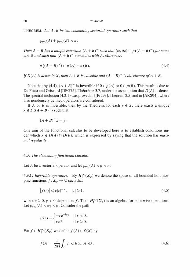
THEOREM. Let A, B be two commuting sectorial operators such that

ϕsec(A)+ ϕsec(B) < π.

Then A+B has a unique extension (A+B)∼ such that (ω,∞)⊂ ρ((A+B)∼) for someω ∈R and such that (A+B)∼ commutes with A. Moreover,

σ((A+B)∼

)⊂ σ(A)+ σ(B). (4.4)

If D(A) is dense in X, then A+B is closable and (A+B)∼ is the closure of A+B .

Note that by (4.4), (A+ B)∼ is invertible if 0 ∈ ρ(A) or 0 ∈ ρ(B). This result is due toDa Prato and Grisvard [DPG75], Théorème 3.7, under the assumption that D(A) is dense.The spectral inclusion (4.2.1) was proved in [[Prü93], Theorem 8.5] and in [ARS94], wherealso nondensely defined operators are considered.

If A or B is invertible, then by the Theorem, for each y ∈ X, there exists a uniquex ∈D((A+B)∼) such that

(A+B)∼x = y.

One aim of the functional calculus to be developed here is to establish conditions un-der which x ∈ D(A) ∩ D(B), which is expressed by saying that the solution has maxi-mal regularity.

4.3. The elementary functional calculus

Let A be a sectorial operator and let ϕsec(A) < ϕ < π .

4.3.1. Invertible operators. By H∞1 (Σϕ) we denote the space of all bounded holomor-

phic functions f :Σϕ →C such that∣∣f (z)∣∣� c|z|−γ , |z|� 1, (4.5)

where c � 0, γ > 0 depend on f . Then H∞1 (Σϕ) is an algebra for pointwise operations.

Let ϕsec(A) < ϕ1 < ϕ. Consider the path

Γ (r)={−re−iϕ1 if r < 0,

reiϕ1 if r � 0.

For f ∈H∞1 (Σϕ) we define f (A) ∈L(X) by

f (A)= 1

2π i

∫Γ

f (λ)R(λ,A)dλ. (4.6)


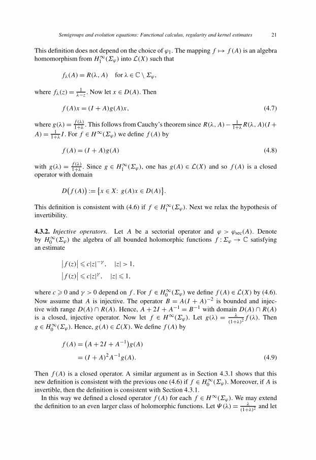
This definition does not depend on the choice of ϕ1. The mapping f �→ f (A) is an algebrahomomorphism from H∞

1 (Σϕ) into L(X) such that

fλ(A)=R(λ,A) for λ ∈C \Σϕ,

where fλ(z)= 1λ−z

. Now let x ∈D(A). Then

f (A)x = (I +A)g(A)x, (4.7)

where g(λ)= f (λ)1+λ

. This follows from Cauchy’s theorem since R(λ,A)− 11+λ

R(λ,A)(I +A)= 1

1+λI . For f ∈H∞(Σϕ) we define f (A) by

f (A)= (I +A)g(A) (4.8)

with g(λ) = f (λ)1+λ

. Since g ∈ H∞1 (Σϕ), one has g(A) ∈ L(X) and so f (A) is a closed

operator with domain

D(f (A)

) := {x ∈X: g(A)x ∈D(A)}.

This definition is consistent with (4.6) if f ∈ H∞1 (Σϕ). Next we relax the hypothesis of

invertibility.

4.3.2. Injective operators. Let A be a sectorial operator and ϕ > ϕsec(A). Denoteby H∞

0 (Σϕ) the algebra of all bounded holomorphic functions f :Σϕ → C satisfyingan estimate∣∣f (z)

∣∣� c|z|−γ , |z|> 1,∣∣f (z)∣∣� c|z|γ , |z|� 1,

where c � 0 and γ > 0 depend on f . For f ∈H∞0 (Σϕ) we define f (A) ∈ L(X) by (4.6).

Now assume that A is injective. The operator B = A(I + A)−2 is bounded and injec-tive with range D(A) ∩ R(A). Hence, A+ 2I + A−1 = B−1 with domain D(A) ∩ R(A)

is a closed, injective operator. Now let f ∈ H∞(Σϕ). Let g(λ) = λ

(1+λ)2 f (λ). Theng ∈H∞

0 (Σϕ). Hence, g(A) ∈ L(X). We define f (A) by

f (A)= (A+ 2I +A−1)g(A)

= (I +A)2A−1g(A). (4.9)

Then f (A) is a closed operator. A similar argument as in Section 4.3.1 shows that thisnew definition is consistent with the previous one (4.6) if f ∈H∞

0 (Σϕ). Moreover, if A isinvertible, then the definition is consistent with Section 4.3.1.

In this way we defined a closed operator f (A) for each f ∈H∞(Σϕ). We may extendthe definition to an even larger class of holomorphic functions. Let Ψ (λ)= λ

(1+λ)2 and let

22 W. Arendt

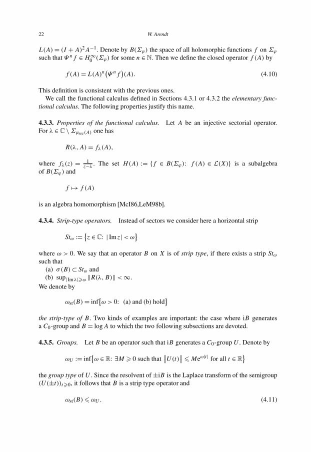
L(A)= (I +A)2A−1. Denote by B(Σϕ) the space of all holomorphic functions f on Σϕ

such that Ψ nf ∈H∞0 (Σϕ) for some n ∈N. Then we define the closed operator f (A) by

f (A)= L(A)n(Ψ nf

)(A). (4.10)

This definition is consistent with the previous ones.We call the functional calculus defined in Sections 4.3.1 or 4.3.2 the elementary func-

tional calculus. The following properties justify this name.

4.3.3. Properties of the functional calculus. Let A be an injective sectorial operator.For λ ∈C \Σϕsec(A) one has

R(λ,A)= fλ(A),

where fλ(z) = 1z−λ

. The set H(A) := {f ∈ B(Σϕ): f (A) ∈ L(X)} is a subalgebraof B(Σϕ) and

f �→ f (A)

is an algebra homomorphism [McI86,LeM98b].

4.3.4. Strip-type operators. Instead of sectors we consider here a horizontal strip

Stω :={z ∈C: | Imz|<ω

}where ω > 0. We say that an operator B on X is of strip type, if there exists a strip Stωsuch that

(a) σ(B)⊂ Stω and(b) sup| Imλ|�ω ‖R(λ,B)‖<∞.

We denote by

ωst(B)= inf{ω > 0: (a) and (b) hold

}the strip-type of B . Two kinds of examples are important: the case where iB generatesa C0-group and B = logA to which the two following subsections are devoted.

4.3.5. Groups. Let B be an operator such that iB generates a C0-group U . Denote by

ωU := inf{ω ∈R: ∃M � 0 such that

∥∥U(t)∥∥� Meω|t | for all t ∈R

}the group type of U . Since the resolvent of ±iB is the Laplace transform of the semigroup(U(±t))t�0, it follows that B is a strip type operator and

ωst(B) � ωU . (4.11)


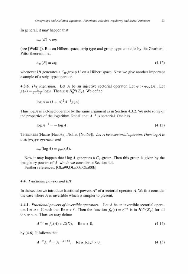
In general, it may happen that

ωst(B) < ωU

(see [Wol81]). But on Hilbert space, strip type and group type coincide by the Gearhart–Prüss theorem; i.e.,

ωst(B)= ωU (4.12)

whenever iB generates a C0-group U on a Hilbert space. Next we give another importantexample of a strip-type operator.

4.3.6. The logarithm. Let A be an injective sectorial operator. Let ϕ > ϕsec(A). Letg(λ)= λ

(1+λ)2 logλ. Then g ∈H∞0 (Σϕ). We define

logA= (I +A)2A−1g(A).

Thus logA is a closed operator by the same argument as in Section 4.3.2. We note some ofthe properties of the logarithm. Recall that A−1 is sectorial. One has

logA−1 =− logA. (4.13)

THEOREM (Haase [Haa03a], Nollau [Nol69]). Let A be a sectorial operator. Then logA isa strip-type operator and

ωst(logA)= ϕsec(A).

Now it may happen that i logA generates a C0-group. Then this group is given by theimaginary powers of A, which we consider in Section 4.4.

Further references: [Oka99,Oka00a,Oka00b].

4.4. Fractional powers and BIP

In the section we introduce fractional powers Aα of a sectorial operator A. We first considerthe case where A is invertible which is simpler to present.

4.4.1. Fractional powers of invertible operators. Let A be an invertible sectorial opera-tor. Let α ∈ C such that Reα > 0. Then the function fα(z) = z−α is in H∞

1 (Σϕ) for all0 < ϕ < π . Thus we may define

A−α = fα(A) ∈ L(X), Reα > 0, (4.14)

by (4.6). It follows that

A−αA−β =A−(α+β), Reα,Reβ > 0. (4.15)

24 W. Arendt

In fact, (A−α)Reα>0 is a bounded holomorphic semigroup. Its generator is − logA (whichwas defined in Section 4.3.6). The operator A is densely defined if and only if logA is so(i.e., if and only if (A−α)Reα>0 is a C0-semigroup).

A particular case of Section 4.4.1 occurs when −A generates an exponentially stableC0-semigroup T (i.e., ‖T (t)‖ � Me−εt for all t � 0 and some M � 0, ε > 0). Then A isinvertible and A−α can be expressed in terms of the semigroup instead of the resolvent asabove, namely,

A−α = 1

Γ (α)

∫ ∞

0tα−1T (t)dt (4.16)

for Reα > 0.Next we consider a more general class of sectorial operators.

4.4.2. Fractional powers of injective sectorial operators. Let A be an injective sectorialoperator and let π > ϕ > ϕsec(A). Let α ∈C, fα(z)= zα , z ∈Σϕ . Then fα ∈B(Σϕ). Thus

Aα = fα(A), α ∈C,

is defined according to Section 4.3.2. It is a closed injective operator and the followingproperties are valid:

A−α = (Aα)−1 = (Aα

)−1, α ∈C; (4.17)

AαAβ ⊂Aα+β, α,β ∈C; (4.18)

AαAβ =Aα+β, Reα,Reβ > 0. (4.19)

If Reα > 0, then

D((A+ω)α

)=D(Aα)

for all ω � 0. (4.20)

Moreover, for 0 < α < πϕsec(A)

, the operator Aα is sectorial and

ϕsec(Aα)= αϕsec(A) and log

(Aα)= α logA; (4.21)

moreover,(Aα)β =Aαβ, Reβ > 0. (4.22)

Formula (4.21) is interesting: it shows in particular that −Aα generates a bounded holo-morphic semigroup if 0 < α is small enough.

There is an enormous amount of literature on fractional powers and we refer in particularto the recent monograph [[MS01]].

Next we consider imaginary powers Ais of an injective sectorial operator. They play animportant role for regularity theory and also for interpolation theory.


4.4.3. Characterization of BIP. Let A be a sectorial injective operator on X. Then bySection 4.4.2 we can define the closed operators Ais , s ∈ R, and also the closed operatorlogA (by Section 4.3.6).

THEOREM. The following assertions are equivalent:(i) D(A) ∩R(A) is dense and Ais ∈L(X) for all s ∈R.

(ii) The operator i logA generates a C0-group U .In that case U(s)=Ais , s ∈R.

DEFINITION. We say that A has bounded imaginary powers and write A ∈ BIP, if A isinjective, sectorial and if the two equivalent conditions of Theorem are satisfied.

Note that this includes the hypothesis that D(A)∩R(A) be dense in X. Recall however,that D(A)∩R(A) is automatically dense in X if X is reflexive and A is a sectorial, injectiveoperator. It is obvious that

A ∈ BIP if and only if A−1 ∈ BIP, (4.23)

References: [Haa03a], [[Prü93]].

4.4.4. BIP for invertible operators. Property BIP can be formulated in a different way ifthe operator is invertible. Let A be sectorial of dense domain. Assume that 0 ∈ ρ(A). Then,for Reα > 0, the operator A−α ∈L(X) was defined in Section 4.4.1, and we had seen that(A−α)Reα>0 is a holomorphic C0-semigroup which is bounded on Σϕ for each 0 < ϕ < π

2 .The generator of this semigroup is − logA. Now it follows from Section 2.3 that A ∈ BIPif and only if the holomorphic C0-semigroup (A−α)Reα>0 has a trace. We formulate thisas a theorem.

THEOREM. Let A be a sectorial densely defined operator with 0 ∈ ρ(A). The followingassertion are equivalent:

(i) A ∈ BIP;(ii) there exists c > 0 such that ‖A−α‖� c whenever Reα > 0, |α|� 1.

4.4.5. The BIP-type. Let A ∈ BIP. Then we denote by

ϕbip(A)= inf{ω ∈R: ∃M � 0 such that

∥∥Ais∥∥� Meω|s| for all s ∈R

}the group-type of the C0-group (Ais)s∈R. We call ϕbip(A) the BIP-type of A. One al-ways has

ϕsec(A) � ϕbip(A). (4.24)

Recall from (4.10) that ϕsec(A) = ωst(logA). If X is a Hilbert space, then ωst(logA) =ϕbip(A) (by (4.12)). Thus we obtain

ϕbip(A)= ϕsec(A) on Hilbert space. (4.25)

26 W. Arendt

This is McIntosh’s result with a new proof due to Haase. The identity (4.25) is no longertrue on Banach spaces. Recently, an example is given by Haase [Haa03a,Haa03b] where

ϕsec(A) < π < ϕbip(A) on a UMD-space X. (4.26)

In fact, X = Lp(R,ω1 dx) ∩ Lq(R,ω2 dx) for 1 < p < 2 < q <∞ and ω1,ω2 strictlypositive measurable functions. Another example of different sectorial and BIP-angle isgiven independently by Kalton [Kal03], where the operator has a bounded H∞-calculus,in addition.

4.4.6. An inverse theorem for BIP operators. If A ∈ BIP, then (Ais)s∈R is a C0-group.Which groups occur in this manner? There is a very satisfying answer if the underlyingBanach space has some geometric properties. We refer to Section 6.1.3 for the definitionof UMD-spaces. Here we just recall that each space Lp,1 <p <∞, is a UMD-space. Let(U(s))s∈R be a C0-group with generator iB . Then B is a strip-type operator. Recall thedefinition of ωst(B) from Section 4.3.4.

THEOREM (Monniaux). Let iB be the generator of a C0-group U on a UMD-space X.Assume that

ωst(B) < π.

Then there exists a unique sectorial operator A such that Ais = U(s) for all s ∈ R.We call A the analytic generator of U .

This theorem is due to Monniaux [Mon99] for the case where ωU < π (the group-type of U). It was Haase [Haa03b] who observed that the weaker assumption ωst(B) < π

suffices. Of course, in the situation of the theorem one has B = logA. One may ask moregenerally which strip type operators B are of the form logA for some sectorial operator A.This seems to be unknown. It is known though, that the hypothesis on the Banach spacecannot be omitted in the above theorem (see [Mon99] for an example). More precisely,on each Banach space X, to each C0-group U one can associate the analytic generator A.If A is sectorial, then Ais =U(s), s ∈R. But if the space X is not a UMD-space, then it mayhappen that ρ(A)= ∅. In particular, A is not sectorial. The notion of analytic generatorsis due to Cioranescu and Zsidó [CZ76] before the notion and properties of UMD-spaceswere known. Their aim was to treat Tomita–Takesaki theory for von Neumann algebras.

4.4.7. Bounded analytic generators. We now describe when the C0-group (Ais)s∈R isthe boundary group of a holomorphic semigroup (see Section 2.3 for this notion).

PROPOSITION [Mon99]. Let U be a C0-group of type < π on a UMD-space X. The fol-lowing assertions are equivalent:

(i) The analytic generator A of U is bounded;(ii) there exists a holomorphic C0-semigroup (T (z))Rez>0 such that U(t)x =

limr↓0 T (it + r)x for all x ∈X.In that case one has A= T (1).


4.4.8. The Dore–Venni theorem. Next we establish the famous Dore–Venni theo-rem [DoVe87] on maximal regularity. It gives an answer to the question of closednessof A + B which arose in Section 4.2. We refer to Section 6.1.3 for the definition andproperties of UMD-spaces.

The following version of the Dore–Venni theorem is due to Prüss and Sohr [PS90].

THEOREM. Let X be a UMD-space. Let A,B ∈ BIP such that ϕbip(A) + ϕbip(B) < π .Assume that A and B commute. Then A+B is closed. Moreover, A+B ∈ BIP and

ϕbip(A+B) � max{ϕbip(A),ϕbip(B)

}.

If one of the operators is invertible, it is possible to deduce this result from Monniaux’inverse theorem (Section 4.4.6). We sketch the proof.

PROOF [MON99]. Assume that 0 ∈ ρ(B). Then by Section 4.4.7 the group (B−is)s∈R isthe boundary of a holomorphic C0-semigroup T and B−1 = T (1). Let W(t)=AitB−it . ByMonniaux’ inverse theorem there exists a sectorial operator C such that Cit =AitB−it . It isnot difficult to show that C =AB−1 with domain D(C)= {x ∈X: B−1x ∈D(A)}. In par-ticular, (AB−1 + I) is invertible. Let y ∈X. We have to find x ∈D(A)+D(B) such thatAx +Bx = y; i.e., (AB−1 + I)Bx = y . Thus x = B−1(AB−1 + I)−1y is a solution. �

4.4.9. A noncommutative Dore–Venni theorem. The assumption that A and B commutecan be relaxed by imposing a growth condition on the commutator of the resolvent.

THEOREM (Monniaux and Prüss [MP97]). Assume that X is a UMD-space. LetA, B ∈ BIP with ϕbip(A) + ϕbip(B) < π . Assume that 0 ∈ ρ(A). Let ψA > ϕbip(A),ψB > ϕbip(B) be angles such that ψA + ψB < π . Assume that there exist constants0 � α < β < 1 and c � 0 such that∥∥AR(λ,A)

[A−1R(μ,B)−R(μ,B)A−1]∥∥� c

(1+ |λ|1−α)|μ|1+β

for all λ ∈Σπ−ψA and all μ ∈Σπ−ψB . Then there exists ω ∈ R such that A+ B + ω isclosed and sectorial.

This result can be applied to Volterra equations [MP97], to nonautonomous evolu-tion equations [HM00a,HM00b] and also to prove maximal regularity of the Ornstein–Uhlenbeck operator [MPRS00].

4.4.10. Interpolation spaces and BIP. Let A be an injective sectorial operator. ThenD(Aα) is a Banach space for the norm

‖x‖D(Aα) := ‖x‖+∥∥Aαx

∥∥,0 < α < 1.

28 W. Arendt

PROPOSITION ([[Tri95], p. 103], [Yag84], [[MS01], Theorem 11.6.1]). Let A ∈ BIP. Thenthe complex interpolation space [X,D(A)]α is isomorphic to D(Aα) for 0 < α < 1.

Now assume in addition that A is invertible. Then Dore [Dor99a] (see also [Dor99b]for the noninvertible case) showed that the part of A in the real interpolation space(X,D(A))α,p has a bounded H∞-calculus whenever 0 < α < 1, 1 < p <∞. (See Sec-tion 4.5 for the definition of H∞-calculus.) If X is a Hilbert space, then (X,D(A))α,2 =[X,D(A)]α. Thus, if X is a Hilbert space, the part of A in [X,D(A)]α has a boundedH∞-calculus. Observe that the part of A in D(Aα) is similar to A. Thus, if D(Aα) =[X,D(A)]α, then A has a bounded H∞-calculus.

We have proved the converse of the above proposition and may formulate the followingcharacterization on Hilbert spaces.

THEOREM. Let A be a sectorial, invertible operator on a Hilbert space and let 0 < α < 1.The following assertions are equivalent:

(i) A ∈ BIP;(ii) D(Aα)= [X,D(A)]α ;

(iii) the H∞-calculus is bounded.

For further results on Hilbert spaces we refer to Section 5 and to the paper by Auscher,McIntosh and Nahmrod [AMN97].

This interesting relation between BIP and interpolation spaces seemed to be the mo-tivation of much research on operators with bounded imaginary powers in the seventies(see, e.g., Seeley’s paper [See67]). Long time after this, the Dore–Venni theorem lead to adifferent direction, namely regularity theory.

4.5. Bounded H∞-calculus for sectorial operators

Let A be an injective sectorial operator on a Banach space X and let π � ϕ > ϕsec(A).Then for f ∈H∞(Σϕ) the closed operator f (A) was defined in Section 4.3.

DEFINITION. We say that A has a bounded H∞(Σϕ)-calculus if

f (A) ∈ L(X) for all f ∈H∞(Σϕ). (4.27)

In that case, the mapping

f �→ f (A)

is a continuous algebra homomorphism from H∞(Σϕ) into L(X).

We note the following: Let ϕsec(A) < ϕ1 < ϕ2 � π . If A has a bounded H∞(Σϕ1)-cal-culus then also the H∞(Σϕ2)-calculus is bounded. Thus, the weakest property in this con-text is to have a bounded H∞(Σπ)-calculus for the cut plane Σπ =C \ {x ∈R: x < 0}.


DEFINITION. We write A ∈ H∞ to say that A is injective, sectorial and has a boundedH∞(Σπ )-calculus. We let

ϕH∞(A) := inf{σ ∈ (ϕsec(A),π

]: A has a bounded H∞(Σϕ)-calculus

}.

4.5.1. Characterization via H∞0 . Let A be an injective sectorial operator with dense do-

main and dense range, and let ϕ > ϕsec(A). Then A has a bounded H∞(Σϕ)-calculus ifand only if there exists c > 0 such that∥∥f (A)

∥∥L(X)� c‖f ‖H∞(Σϕ) (4.28)

for all f ∈ H∞0 (Σϕ). Note that H∞

0 (Σϕ) is not norm-dense in H∞(Σϕ). Still, there isa canonical way to extend the calculus.

4.5.2. Unbounded H∞-calculus. It is not an easy matter to decide whether a given oper-ator has a bounded H∞-calculus. Later we will give several criteria and examples. Here weshow a way to construct counterexamples. Let X be a Banach space. A sequence (en)n∈N iscalled a Schauder basis of X if, for each x ∈X, there exists a unique sequence (xn)n∈N ⊂C

such that

∞∑n=1

xnen = x. (4.29)

The Schauder basis is called unconditional if for each x =∑∞n=1 xnen ∈ X the sequence∑∞

n=1 cnxnen converges in X for each c= (cn)n∈N ∈ �∞. Otherwise we call (en)n∈N a con-ditional Schauder basis. If X has an unconditional Schauder basis it also has a conditionalSchauder basis [[Sin70], Chapter II, Theorem. 23.2]. In particular, each separable Hilbertspace has a conditional Schauder basis. Thus the following example is in particular validin a separable Hilbert space.

EXAMPLE (Unbounded H∞(Σπ )-calculus). Let X be a Banach space with a conditionalSchauder basis (en)n∈N. Define the operator A on X by

Ax =∞∑n=1

2nxnen (4.30)

with domain the set of all x =∑∞n=1 xnen ∈ X such that (4.30) converges. Then A is

sectorial with ϕsec(A)= 0. However, A does not have a bounded H∞(Σπ )-calculus.

For the proof it is helpful to consider more general diagonal operators. Denote by BVthe space of all scalar sequences α = (αn)n∈N such that

‖α‖BV = |α1| +∞∑n=1

|αn+1 − αn|<∞.

30 W. Arendt

Then BV is a Banach space (isomorphic to �1). If∑∞

n=1 yn converges in X, then∑∞n=1 αnyn converges for each α ∈ BV . This follows from Abel’s partial summation rule

m∑n=1

αnyn =m∑

n=1

αn(sn+1 − sn)=m∑

n=2

sn(αn−1 − αn)+ sm+1αm − s1α1,

where s1 = 0, sn =∑n−1k=1 yk for n � 2. Thus, if α ∈ BV , then

Dαx =∞∑n=1

αnxnen (4.31)

for x =∑∞n=1 xnen defines an operator Dα ∈ L(X). Moreover,

‖Dα‖� c‖α‖BV , α ∈BV, (4.32)

by the closed graph theorem (or a direct estimate). Next we consider unbounded diagonaloperators. Let (αn)n∈N ⊂C. Then

Dαx =∞∑n=1

αnxnen (4.33)

with D(Dα) := {x =∑∞n=1 xnen: (4.33) converges} defines a closed operator on X. This

is obvious since the coordinate functionals

∞∑n=1

xnen �→ xm

are continuous.

PROPOSITION. Let 0 < α1 < αn < αn+1 such that limn→∞ αn =∞. Then Dα is a sector-ial operator of type ϕsec(Dα)= 0. Moreover, 0 ∈ ρ(Dα) and Dα has compact resolvent.

PROOF. Let 0 < ϕ < π . Let π � |θ | > ϕ, λ = reiθ , r > 0. Consider the sequenceβn = 1

reiθ−αn. Then

βn − βn+1 = 1

r

{1

eiθ − αn/r− 1

eiθ − αn+1/r

},

∞∑n=1

|βn − βn+1|� 1

r

∞∑n=1

∫ αn+1/r

αn/r

1

|eiθ − x|2 dx

� 1

r

∫ ∞

0

1

|eiθ − x|2 dx = cϕ

r,


where cϕ does not depend on θ or r . Thus ‖Dβ‖ � cr. It is easy to see that Dβ =

(λ − Dα)−1. This shows that Dα is sectorial of type 0. We omit the proof of compact-

ness of Dβ (see [LeM00]). �

Now let A be the operator of the example; i.e., A = Dα with αn = 2n. In order toshow that A has no bounded H∞(Σπ )-calculus we use the following (see [[Gar81], The-orem 1.1. on pp. 287 and 284 ff ]).

INTERPOLATION LEMMA. Let b = (bn)n∈Z ∈ �∞(Z). Then there exists f ∈ H∞(Σπ )

such that

f(2n)= bn for all n ∈ Z.

Let f ∈H∞(Σπ). It is easy to see from the definition that en ∈D(f (A)) and

f (A)en = f(2n)en.

Now assume that f (A) ∈ L(X). Then it follows that

limm→∞

m∑n=1

f(2n)xnen = lim

m→∞f (A)

m∑n=1

xnen

= f (A)x

converges for all x ∈ X. Thus, by the Interpolation Lemma,∑∞

n=1 bnxnen converges forall b ∈ �∞ and all x ∈X. This contradicts the fact that the basis is conditional.

A first example of this kind had been given by Baillon and Clément [BC91]. Furtherdevelopments are contained in [Ven93], [LeM00] and [Lan98].

4.5.3. BIP versus bounded H∞-calculus. It is clear from the definition that A ∈ H∞implies A ∈ BIP whenever A is a sectorial, injective operator. It is remarkable that inthat case

ϕbip(A)= ϕH∞(A) (4.34)

(see [CDMY96]). Conversely, if X is a Hilbert space, then BIP implies boundedness of theH∞-calculus by Section 4.4.10. This is not true on Lp-spaces for p �= 2 as the followingexample shows.

EXAMPLE [Lan98]. Let 1 < p < ∞, p �= 2. There exists a sectorial injective opera-tor A ∈ BIP on Lp which does not have a bounded H∞(Σπ )-calculus. We considerthe space L

p

2π of all scalar-valued 2π -periodic measurable functions on R such that

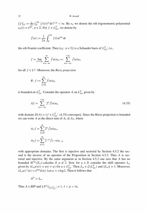
32 W. Arendt

‖f ‖p := 12π (∫ 2π

0 |f (t)|p dt)1/p <∞. By en we denote the nth trigonometric polynomialen(t)= eint , n ∈ Z. For f ∈L

p2π , we denote by

f (n) := 1

2π

∫ 2π

0f (t)eint dt

the nth Fourier coefficient. Then {en: n ∈ Z} is a Schauder basis of Lp

2π ; i.e.,

f = limn→∞

m∑n=−m

f (n)en =:+∞∑

n=−∞f (n)en

for all f ∈Lp . Moreover, the Riesz-projection

R :f �→∞∑n=0

f (n)en

is bounded on Lp

2π . Consider the operator A on Lp

2π given by

Af =+∞∑

n=−∞2nf (n)en (4.35)

with domain D(A)= {f ∈ Lp

2π : (4.35) converges}. Since the Riesz-projection is boundedwe can write A as the direct sum of A1 ⊕A2, where

A1f =∞∑n=0

2nf (n)en,

A2f =∞∑n=1

2−nf (−n)e−n

with appropriate domains. The first is injective and sectorial by Section 4.5.2 the sec-ond is the inverse of an operator of the Proposition in Section 4.5.2. Thus A is sec-torial and injective. By the same argument as in Section 4.5.2 one sees that A has nobounded H∞(Σπ)-calculus if p �= 2. Now for a ∈ R consider the shift operator La

given by (Lau)(t)= u(t + a) for u ∈ Lp

2π . Then La ∈ L(Lp

2π ) and ‖La‖ = 1. Moreover,(Lau)

∧(n)= einau(n). Let a = s log 2. Then it follows that

Ais = La.

Thus A ∈ BIP and ‖Ais‖L(Lp

2π )= 1, 1 <p <∞.


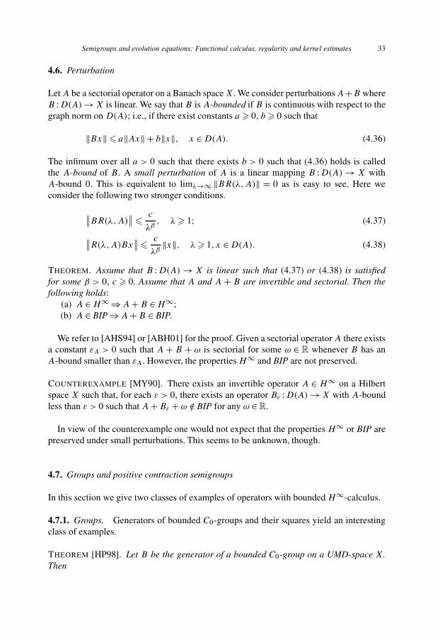
4.6. Perturbation

Let A be a sectorial operator on a Banach space X. We consider perturbations A+B whereB :D(A)→X is linear. We say that B is A-bounded if B is continuous with respect to thegraph norm on D(A); i.e., if there exist constants a � 0, b � 0 such that

‖Bx‖� a‖Ax‖+ b‖x‖, x ∈D(A). (4.36)

The infimum over all a > 0 such that there exists b > 0 such that (4.36) holds is calledthe A-bound of B . A small perturbation of A is a linear mapping B :D(A)→ X withA-bound 0. This is equivalent to limλ→∞‖BR(λ,A)‖ = 0 as is easy to see. Here weconsider the following two stronger conditions.∥∥BR(λ,A)

∥∥� c

λβ, λ � 1; (4.37)∥∥R(λ,A)Bx

∥∥� c

λβ‖x‖, λ � 1, x ∈D(A). (4.38)

THEOREM. Assume that B :D(A)→ X is linear such that (4.37) or (4.38) is satisfiedfor some β > 0, c � 0. Assume that A and A+ B are invertible and sectorial. Then thefollowing holds:

(a) A ∈H∞⇒A+B ∈H∞;(b) A ∈ BIP⇒A+B ∈ BIP.

We refer to [AHS94] or [ABH01] for the proof. Given a sectorial operator A there existsa constant εA > 0 such that A + B + ω is sectorial for some ω ∈ R whenever B has anA-bound smaller than εA. However, the properties H∞ and BIP are not preserved.

COUNTEREXAMPLE [MY90]. There exists an invertible operator A ∈ H∞ on a Hilbertspace X such that, for each ε > 0, there exists an operator Bε :D(A)→X with A-boundless than ε > 0 such that A+Bε +ω /∈ BIP for any ω ∈R.

In view of the counterexample one would not expect that the properties H∞ or BIP arepreserved under small perturbations. This seems to be unknown, though.

4.7. Groups and positive contraction semigroups

In this section we give two classes of examples of operators with bounded H∞-calculus.

4.7.1. Groups. Generators of bounded C0-groups and their squares yield an interestingclass of examples.

THEOREM [HP98]. Let B be the generator of a bounded C0-group on a UMD-space X.Then

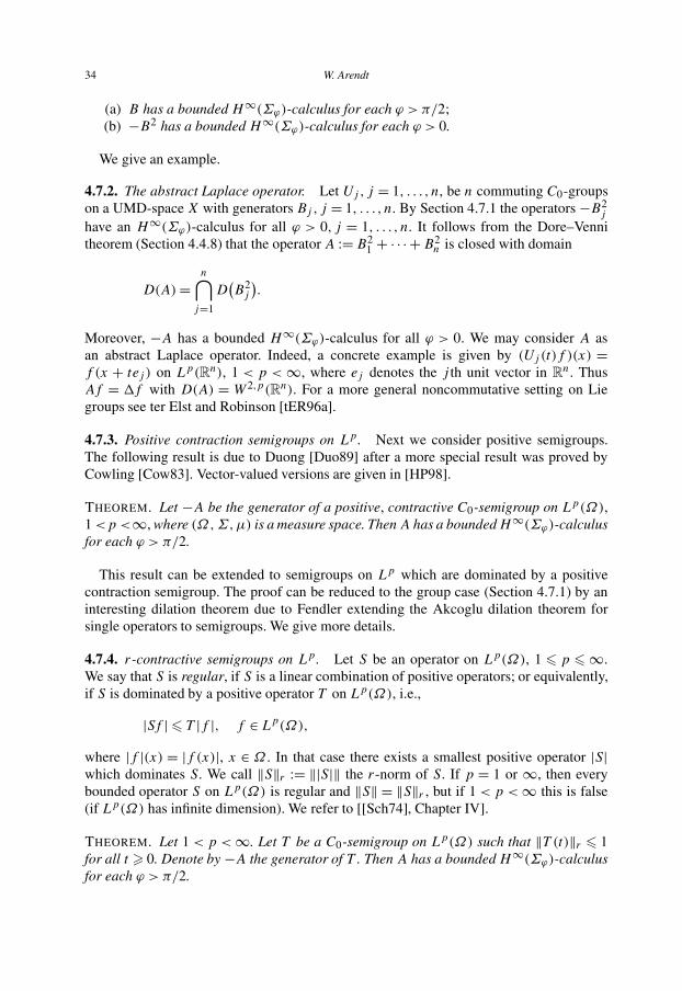
34 W. Arendt

(a) B has a bounded H∞(Σϕ)-calculus for each ϕ > π/2;(b) −B2 has a bounded H∞(Σϕ)-calculus for each ϕ > 0.

We give an example.

4.7.2. The abstract Laplace operator. Let Uj , j = 1, . . . , n, be n commuting C0-groupson a UMD-space X with generators Bj , j = 1, . . . , n. By Section 4.7.1 the operators −B2

j

have an H∞(Σϕ)-calculus for all ϕ > 0, j = 1, . . . , n. It follows from the Dore–Vennitheorem (Section 4.4.8) that the operator A := B2

1 + · · · +B2n is closed with domain

D(A)=n⋂

j=1

D(B2

j

).

Moreover, −A has a bounded H∞(Σϕ)-calculus for all ϕ > 0. We may consider A asan abstract Laplace operator. Indeed, a concrete example is given by (Uj (t)f )(x) =f (x + tej ) on Lp(Rn), 1 < p <∞, where ej denotes the j th unit vector in Rn. ThusAf = �f with D(A) = W 2,p(Rn). For a more general noncommutative setting on Liegroups see ter Elst and Robinson [tER96a].

4.7.3. Positive contraction semigroups on Lp . Next we consider positive semigroups.The following result is due to Duong [Duo89] after a more special result was proved byCowling [Cow83]. Vector-valued versions are given in [HP98].

THEOREM. Let −A be the generator of a positive, contractive C0-semigroup on Lp(Ω),1 <p <∞, where (Ω,Σ,μ) is a measure space. Then A has a boundedH∞(Σϕ)-calculusfor each ϕ > π/2.

This result can be extended to semigroups on Lp which are dominated by a positivecontraction semigroup. The proof can be reduced to the group case (Section 4.7.1) by aninteresting dilation theorem due to Fendler extending the Akcoglu dilation theorem forsingle operators to semigroups. We give more details.

4.7.4. r-contractive semigroups on Lp . Let S be an operator on Lp(Ω), 1 � p �∞.We say that S is regular, if S is a linear combination of positive operators; or equivalently,if S is dominated by a positive operator T on Lp(Ω), i.e.,

|Sf |� T |f |, f ∈ Lp(Ω),

where |f |(x) = |f (x)|, x ∈ Ω . In that case there exists a smallest positive operator |S|which dominates S. We call ‖S‖r := ‖|S|‖ the r-norm of S. If p = 1 or ∞, then everybounded operator S on Lp(Ω) is regular and ‖S‖ = ‖S‖r , but if 1 < p <∞ this is false(if Lp(Ω) has infinite dimension). We refer to [[Sch74], Chapter IV].

THEOREM. Let 1 < p <∞. Let T be a C0-semigroup on Lp(Ω) such that ‖T (t)‖r � 1for all t � 0. Denote by −A the generator of T . Then A has a bounded H∞(Σϕ)-calculusfor each ϕ > π/2.


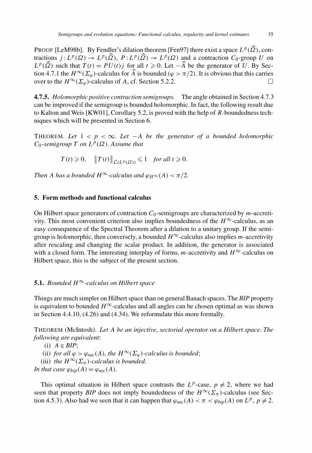
PROOF [LeM98b]. By Fendler’s dilation theorem [Fen97] there exist a space Lp(Ω), con-tractions j :Lp(Ω)→ Lp(Ω), P :Lp(Ω)→ Lp(Ω) and a contraction C0-group U onLp(Ω) such that T (t) = PU(t)j for all t � 0. Let −A be the generator of U . By Sec-tion 4.7.1 the H∞(Σϕ)-calculus for A is bounded (ϕ > π/2). It is obvious that this carriesover to the H∞(Σϕ)-calculus of A, cf. Section 5.2.2. �

4.7.5. Holomorphic positive contraction semigroups. The angle obtained in Section 4.7.3can be improved if the semigroup is bounded holomorphic. In fact, the following result dueto Kalton and Weis [KW01], Corollary 5.2, is proved with the help of R-boundedness tech-niques which will be presented in Section 6.

THEOREM. Let 1 < p < ∞. Let −A be the generator of a bounded holomorphicC0-semigroup T on Lp(Ω). Assume that

T (t) � 0,∥∥T (t)

∥∥L(Lp(Ω))� 1 for all t � 0.

Then A has a bounded H∞-calculus and ϕH∞(A) < π/2.

5. Form methods and functional calculus

On Hilbert space generators of contraction C0-semigroups are characterized by m-accreti-vity. This most convenient criterion also implies boundedness of the H∞-calculus, as aneasy consequence of the Spectral Theorem after a dilation to a unitary group. If the semi-group is holomorphic, then conversely, a bounded H∞-calculus also implies m-accretivityafter rescaling and changing the scalar product. In addition, the generator is associatedwith a closed form. The interesting interplay of forms, m-accretivity and H∞-calculus onHilbert space, this is the subject of the present section.

5.1. Bounded H∞-calculus on Hilbert space

Things are much simpler on Hilbert space than on general Banach spaces. The BIP propertyis equivalent to bounded H∞-calculus and all angles can be chosen optimal as was shownin Section 4.4.10, (4.26) and (4.34). We reformulate this more formally.

THEOREM (McIntosh). Let A be an injective, sectorial operator on a Hilbert space. Thefollowing are equivalent:

(i) A ∈ BIP;(ii) for all ϕ > ϕsec(A), the H∞(Σϕ)-calculus is bounded;

(iii) the H∞(Σπ )-calculus is bounded.In that case ϕbip(A)= ϕsec(A).

This optimal situation in Hilbert space contrasts the Lp-case, p �= 2, where we hadseen that property BIP does not imply boundedness of the H∞(Σπ )-calculus (see Sec-tion 4.5.3). Also had we seen that it can happen that ϕsec(A) < π < ϕbip(A) on Lp , p �= 2.

36 W. Arendt

Also the Dore–Venni theorem needs fewer hypotheses on Hilbert space.

THEOREM (Dore–Venni on Hilbert space [DoVe87]). Let A and B be two commutinginjective, sectorial operators on a Hilbert space such that ϕsec(A)+ ϕsec(B) < π . Assumethat A ∈ BIP. Then A+B is closed.

We mention that this result does not hold on Lp for p �= 2 ([Lan98], Theorem 2.3).

5.2. m-accretive operators on Hilbert space

The simplest unbounded operators are multiplication operators. Let (Ω,Σ,μ) be a mea-sure space and let m :Ω → R be a measurable function. Define Am on L2(Ω) byAmu=mu with domain

D(Am)= {u ∈ L2(Ω): m · u ∈L2(Ω)}.

For the operator Am one has the best possible spectral calculus. For each f ∈ L∞(R),we may define f (A) = Af ◦m ∈ L(L2(Ω)). It is not difficult to see that this definition isconsistent with our previous one whenever f ∈H∞(Σϕ) for some ϕ > π/2.

5.2.1. The Spectral theorem. The spectral theorem says that each self-adjoint operator isunitarily equivalent to a multiplication operator.

SPECTRAL THEOREM. Let A be a self-adjoint operator on H . Then there exists ameasure space (Ω,Σ,μ), a measurable function m :Ω→R and a unitary operatorU :H → L2(Ω) such that

(a) UD(A)=D(Am);(b) AmUx =UAx , x ∈D(A).

Thus, multiplication operators and self-adjoint operators are just the same thing.Now recall that an operator A generates a unitary group (i.e., a C0-group of unitary

operators) if and only if iA is self-adjoint. Thus iA is equivalent to a multiplication opera-tor. This shows in particular that each generator A of a unitary group on H has a boundedH∞(Σϕ)-calculus for all ϕ > π/2. In fact, it is easy to show that for f ∈H∞(Σϕ) one has

f (A)=U−1Af ◦mU.

5.2.2. Bounded H∞-calculus for m-accretive operators. Recall that an operator A ona Hilbert space H is called m-accretive if

(a) Re(Ax|x)� 0 for all x ∈D(A);(b) I +A is surjective.

The Lumer–Phillips theorem asserts that an operator A is m-accretive if and only if−A generates a contractive C0-semigroup. In particular, if A is m-accretive, then A issectorial and ϕsec(A) � π

2 .


THEOREM. Let A be an m-accretive operator on H . Then A has a boundedH∞(Σϕ)-calculus for each ϕ > ϕsec(A).

PROOF. Denote by T the semigroup generated by −A. By the dilation theorem [[Dav80],p. 157] there exist a Hilbert space H containing H as a closed subspace and a unitarygroup U on H such that

P ◦U(t) ◦ i = T (t), t � 0,

where i :H → H is the injection of H into H and P : H → H is the orthogonal pro-jection. Denote by A the generator of U . Then iA is selfadjoint. Thus A has a boundedH∞(Σϕ)-calculus for any ϕ > π/2. It is easy to see from the definitions that

f (A)= P ◦ f (A ) ◦ i.Thus f (A) ∈ L(H) for all f ∈ H∞(Σϕ) (and even ‖f (A)‖ � ‖f (A)‖ � ‖f ‖L∞(Σπ/2)).Thus A has a bounded H∞(Σϕ)-calculus for all ϕ > π

2 . Now by McIntosh’s result inSection 5.1 the H∞(Σϕ)-calculus is also bounded for ϕ > ϕsec(A). �

5.2.3. Equivalence of bounded H∞-calculus and m-accretivity. Let (·|·)1 be an equiva-lent scalar product on H , i.e., there exist α > 0, β > 0 such that

α‖u‖2H � (u|u)1 � β‖u‖2

H

for all u ∈H . Of course, having a bounded H∞-calculus is independent of the equivalentnorm on H we choose. Thus, if A is a sectorial operator on H which is m-accretive withrespect to some equivalent scalar product, then A ∈H∞. This describes already the classof all operators A with bounded H∞-calculus.

THEOREM (Le Merdy [LeM98a]). Let A be an injective, sectorial operator on H suchthat ϕsec(A) < π/2. The following are equivalent:

(i) A ∈H∞,(ii) there exists an equivalent scalar product (·|·)1 on H such that Re(Au|u)1 � 0 for

all u ∈D(A);(iii) let 0 � ϕ < ϕsec(A); then there exists an equivalent scalar product (·|·)1 on H such

that (Au|u) ∈Σϕ for all u ∈D(A).

Denote by T the C0-semigroup generated by −A. Then (ii) means that∥∥T (t)u∥∥

1 � ‖u‖1 :=√(u|u)1

for all u ∈H , t � 0, and (iii) means that∥∥T (z)u∥∥

1 � ‖u‖1

38 W. Arendt

for all u ∈H and z ∈Σπ/2−ϕ .The proof of Le Merdy [LeM98a] uses the theory of completely bounded operators and

a deep theorem of Paulsen. A more direct proof, based directly on “quadratic estimates”,is given by Haase [Haa02].

The theorem gives a very satisfying characterization of the boundedness of theH∞-calculus; see also Section 5.3 for a description by forms. However, it is restrictedto sectorial operators of sectorial type smaller than π/2:

5.2.4. Counterexample. There exists an invertible, sectorial operator A on a Hilbertspace H such that −A generates a bounded C0-semigroup T on H . Moreover, A hasa bounded H∞(Σϕ)-calculus for any ϕ > π/2. But for all ω > 0, A+ ω is not accretivewith respect to any equivalent scalar product.

The counterexample is due to Le Merdy [LeM98a] (based on a famous example of Pisiersolving the Halmos problem) with an additional argument by Haase [Haa02] (taking careof the case where ω > 0).

5.3. Form methods

A most efficient way to define generators of holomorphic semigroups on a Hilbert spaceH is the form method (sometimes it is also called “variational method”).

Let H be a Hilbert space. If V is another Hilbert space we write V ↪→H if V is a sub-space of H such that the embedding is continuous. We write V ↪→d H if in addition V isdense in H .

DEFINITION. A closed form on H is a sesquilinear form a :V × V →C which is contin-uous, i.e., ∣∣a(u, v)∣∣� M‖u‖V ‖v‖V , u, v ∈ V, (5.1)

for some M � 0 and elliptic, i.e.,

Rea(u,u)+ω‖u‖2H � α‖u‖2

V , u ∈ V, (5.2)

for some ω ∈R, α > 0. The space V is called the domain of a.

Properly speaking, a closed form is a couple (a,V ) with the properties stipulated in theabove definition. Note that by (5.2),

‖u‖a :=(Rea(u,u)+ω‖u‖2

H

)1/2

defines an equivalent norm on V . Sometimes we will write D(a) instead of V and will usethe norm ‖ · ‖a on D(a) for which D(a) is complete by hypothesis.


REMARK. Let a :D(a) × D(a)→ C be sesquilinear, where D(a) is a subspace of H .Assume that a is bounded below, i.e.,

‖u‖2a := Rea(u,u)+ω‖u‖2

H � ‖u‖2H

for all u ∈D(a) and some ω ∈R. Then ‖ · ‖a defines a norm on D(a). The form is contin-uous with respect to this norm if and only if a(u,u) ∈ ω1 +Σθ for some ω1 ∈R and someθ ∈ (0,π/2], i.e., if and only if the form a is sectorial in the terminology of Kato [[Kat66]].

5.3.1. The operator associated with a closed form. Let a be a closed form on H withdense domain V . Then we associate an operator A with a, given by

D(A)= {u ∈ V : ∃v ∈H such that a(u,ϕ)= (v|ϕ)H for all ϕ ∈ V},

Au= v.

Note that v is well defined since V is dense in H . We call A the operator associatedwith a. It is not difficult to see that A + ω is sectorial with angle ϕsec(A + ω) < π/2.Moreover, A + ω is m-accretive (where ω is the constant occurring in (5.2)). Thus weobtain the following.

THEOREM. Let A be an operator associated with a closed form. Then there exists ω ∈ R

such that A+ω ∈H∞.

5.3.2. Example: self-adjoint operators. Let a be a densely defined closed form on H

with domain V . Assume that a is symmetric; i.e., a(u, v) = a(v,u) for all u,v ∈ V . LetA be the operator associated with a. Then A is bounded below (i.e., (Au|u) � −ω‖u‖2

H

for all u ∈D(A) and some ω ∈ R) and self-adjoint. Conversely, let A be a self-adjointoperator which is bounded below. Then A is associated with a densely defined symmetricclosed form.

We give a classical concrete example right now. Later we will study elliptic operators inmore detail.

5.3.3. Example (The Laplacian with Dirichlet and with Neumann boundary conditions).Let Ω ⊂ Rn be open and H = L2(Ω). Let W 1,2(Ω) := {u ∈ L2(Ω): Dju ∈ L2(Ω),j = 1, . . . , n} be the first Sobolev space and let W 1,2

0 (Ω) be the closure of the space D(Ω)

of all test functions in W 1,2(Ω). Define a :W 1,2(Ω)×W 1,2(Ω)→C by

a(u, v)=∫Ω

∇u∇v dx.

(a) Let V =W1,20 (Ω). Then a is a closed symmetric form. Denote by −�D

Ω the oper-

ator associated with a. Then it is easy to see that D(�DΩ)= {u ∈W

1,20 (Ω): �u ∈L2(Ω)},

�DΩu=�u, in D(Ω)′. We call �D

Ω the Dirichlet Laplacian on L2(Ω).

40 W. Arendt

(b) Let V = W 1,2(Ω). Then a is closed and symmetric. Denote by −�NΩ the op-

erator associated with a. Then �NΩ is a self-adjoint operator, called the Neumann

Laplacian. This can be justified if Ω is bounded with Lipschitz boundary. ThenD(�N

Ω)= {u ∈W 1,2(Ω): �u ∈L2(Ω); ∂u∂v= 0 weakly}, where the weak sense has to be

explained. We omit the details. And indeed, for many purposes it is not important to knowin which sense the Neumann boundary condition ∂u

∂v= 0 is realized. The interesting point

is that the Neumann–Laplacian can be defined for arbitrary open sets without using thenormal derivative.

5.3.4. Characterization of operators defined by forms. Let A be an operator on H .We say that A is induced by a form, if there exists a densely defined closed form a on H

such that A is associated with a. It is easy to describe such operators by an accretivity-condition.

THEOREM [[Kat66]]. Let A be an operator on H . The following are equivalent:(i) A is induced by a form;

(ii) there exist ω ∈R and 0 < θ < π2 such that

(a) (ω+A)D(A)=H ;(b) e±iθ (ω+A) is accretive.

(iii) −A generates a holomorphic C0-semigroup T of angle θ ∈ (0, π2 ) such that for

some ω ∈R,∥∥T (z)∥∥� eω|z|, z ∈Σθ ;

(iv) the numerical range W(A) := {(Ax|x): x ∈ D(A),‖x‖ = 1} is contained inΣθ +ω for some θ ∈ (0,π/2), ω ∈R and (−∞,ω)∩ ρ(A) �= ∅.

Property (ii) is sometimes formulated by saying that A is strongly quasi-m-accretive(and strongly m-accretive if ω= 0).

5.3.5. Changing scalar products. Let a :V × V → C be a closed densely defined formon H . The definition of the associated operator A depends on the scalar product on H .Let (·|·)1 be another equivalent scalar product on H . Then there exists a self-adjoint oper-ator Q ∈ L(H) such that

(Qu|v)1 = (u|v) for all u,v ∈H,

and Q is strictly form-positive. By this we mean that (Qu|u) � ε‖u‖2H for all u ∈ H and

some ε > 0. Let u ∈D(A). Then u ∈ V and a(u,ϕ)= (Au|ϕ)= (QAu|ϕ)1 for all ϕ ∈ V .This shows that the operator A1 associated with a on (H, (·|·)1) is given by A1 =QA. Withthe help of Le Merdy’s theorem in Section 5.2.3 one obtains the following characterizationof the class H∞.

THEOREM [ABH01]. Let A be an operator on H . The following are equivalent:(i) A+ω ∈H∞ for some ω � 0;


(ii) there exists an equivalent scalar product (·|·)1 on H such that A is induced bya form on (H, (·|·)1);

(iii) there exists a strictly form-positive self-adjoint operator Q ∈ L(H) such that QA

is induced by a form.

We remark that the rescaling A+ ω is needed to obtain a sectorial operator. From Sec-tion 4.6 we know that for an invertible sectorial operator A and ω > 0 one has

A ∈H∞ if and only if A+ω ∈H∞.

5.3.6. More on equivalent scalar products. In the Section 5.3.5 we characterized thoseoperators A which come from a form on (H, (·|·)1) for some equivalent scalar product.What happens if we replace “some” by “all ”?

THEOREM (Matolcsi [Mat03]). Let A be an operator on H . The following are equivalent:(i) A is bounded;

(ii) for each equivalent scalar product (·|·)1 on H , the operator A is induced by a formon (H, (·|·)1).

5.4. Form sums and Trotter’s product formula

There is a natural way to define the sum of closed forms leading to a closed form again.Here we want to allow also nondense form domains. Let H be a Hilbert space.

5.4.1. Closed forms with nondense domain. We define closed forms on H as before butomit the assumption that the form domain be dense in H . Thus, a closed form a on H

is a sesquilinear form a :D(a)× D(a)→ C, where D(a) is a subspace of H (the formdomain) such that, for some ω ∈R, α ∈ [0,π/2):

(a) a(u,u)+ (ω− 1)‖u‖2H ∈Σα , u ∈D(a);

(b) (D(a),‖ · ‖a) is complete, where ‖u‖2a = Rea(u,u)+ω‖u‖2

H .Then one can show that a is a continuous sesquilinear form on V = (D(a),‖ · ‖a). Thus(5.1) and (5.2) are satisfied.

Denote by A the operator on D(a) (the closure of D(a) in H ) associated with a. Then−A generates a holomorphic C0-semigroup (e−tA)t�0 on D(a). We extend this semigroupby 0 to H defining

e−tax :={

e−tAx if x ∈D(a),

0 if x ∈D(a)⊥,(5.3)

for t > 0 and letting e−0a the orthogonal projection onto D(a). Then t �→ e−ta :[0,∞)→ L(H) is strongly continuous and satisfies the semigroup property

e−tae−sa = e−(t+s)a, t, s � 0.

42 W. Arendt

We call (e−ta)t�0 the semigroup on H associated with the closed form a. Before givingexamples we consider form sums.

5.4.2. Form sums. Now let a and b be two closed forms on H . Then D(a) ∩ D(b) isa Hilbert space for the norm (‖u‖2

a + ‖u‖2b)

1/2. Hence, a + b with domain D(a + b) =D(a)∩D(b) is a closed form again.

THEOREM. Let a and b be two closed forms on H . Then Trotter’s formula

e−t (a+b)x = limn→∞

(e−(t/n)ae−(t/n)b

)nx (5.4)

holds for all x ∈H , t � 0.

This result is due to Kato [Kat78] for the case of symmetric forms and it was generalizedto closed forms by Simon (see [Kat78], Theorem and Addendum).

It is interesting that this result can be applied in particular when e−tb ≡ P , where P isan orthogonal projection. This is done in the following section.

5.4.3. Induced semigroups. Let a be a closed form on H . Let H1 be a closed subspaceof H . Even if H1 is not invariant under (e−ta)t�0 there is a natural induced semigroupon H1. In fact, let D(b) = H1 and b ≡ 0. Then e−tb ≡ P , the orthogonal projectiononto H1. Thus by Trotter’s formula (5.4),

e−ta1x = limn→∞

(e−ta/nP

)nx (5.5)

converges for all x ∈ H , where D(a1) = D(a) ∩ H1 and a1(u, v) = a(u, v) for allu,v ∈D(a1). Then (e−ta1)t�0 is a C0-semigroup on H1 if and only if D(a)∩H1 is densein H1.

5.4.4. Nonconvergence of Trotter’s formula. Before giving a concrete example we wantto point out that this way to induce a semigroup on closed subspaces via (5.5) does notwork for arbitrary contraction semigroups.

THEOREM (Matolcsi [Mat03]). Let−A be the generator of a contraction C0-semigroup T

on H . The following assertion are equivalent:(i) A is induced by a form;

(ii) limn→∞(T (t/n)P )nx converges for each t > 0, x ∈H , and each orthogonal pro-jection P .

5.4.5. From the Gaussian semigroup to the Dirichlet Laplacian. Denote by G theGaussian semigroup on L2(Rn), i.e.,

G(t)f (x)= (4πt)−n/2∫

Rn

e−(x−y)2/4tf (y)dy


for all t > 0, f ∈ L2(Rn), x ∈ Rn. Then G is associated with the form a(u, v) =∫Rn ∇u∇v dx with domain D(a)=W 1,2(Rn). Now let Ω ⊂ Rn be an open subset of Rn.

We identify L2(Ω) with the space {f ∈ L2(Rn): f (x) = 0 a.e. on Ωc}. Then the or-thogonal projection P onto L2(Ω) is given by Pf = 1Ωf for all f ∈ L2(Rn). Now letW

1,20 (�Ω) = W 1,2(Rn) ∩ L2(Ω) = {u ∈ W 1,2(Rn): u(x) = 0 a.e. on Ωc}. Consider the

form b on W1,20 (�Ω) given by b(u, v)= ∫

Ω∇u∇v. Then, by (5.5), we have

e−tbf = limn→∞

(G(t/n)1Ω

)nf (5.6)

for all f ∈ L2(Rn). Now we consider the more familiar space W1,20 (Ω). For u ∈W

1,20 (Ω)

let u(x)= u(x) for x ∈Ω and u(x)= 0 for x ∈Ωc. Then u ∈W1,20 (�Ω) and Dj u= Dju.

Thus we may identify W1,20 (Ω) with a subspace of W 1,2

0 (�Ω). One says that Ω is stable, if

W1,20 (Ω)=W

1,20 (�Ω). For example, if Ω has Lipschitz boundary, then Ω is stable. Thus

Ω is stable if and only if (e−tb)t�0 is the semigroup generated by the Dirichlet Laplacianwith the canonical extension to L2(Rn), i.e.,

(e−tbf

)(x)=

{(et�

DΩf∣∣Ω

)(x), x ∈Ω ,

0, x /∈Ω .

Thus, if Ω is stable, then the semigroup generated by the Dirichlet Laplacian is obtainedfrom the Gaussian semigroup via Trotter’s formula (5.6).

Stable open sets can be characterized as follows. Let Ω be an open, bounded set in Rn.We assume that the boundary ∂Ω of Ω is a null-set (for the n-dimensional Lebesgue

measure), and that◦�Ω =Ω . By

cap(A)= inf{‖u‖2

H 1 : u ∈H 1(Rn), u � 1, a.e. in a neighborhood of A

}we denote the capacity of a subset A of Rn.

THEOREM. The following assertions are equivalent.(i) W

1,20 (Ω)=W

1,20 (�Ω);

(ii) cap(G \ �Ω)= cap(G \Ω) for every open set G⊂Rn;(iii) for each function u ∈ C(�Ω), which is harmonic on Ω , there exist un harmonic on

an open neighborhood of �Ω which converge to u uniformly on �Ω as n→∞.

It is interesting that these properties do not imply Dirichlet regularity. In fact, if Ω is theLebesgue cusp, then W

1,20 (Ω)=W

1,20 (�Ω). References: [Hed93] and [Kel66].

44 W. Arendt

5.5. The square root property

Let H be a Hilbert space. During this section we consider a continuous sesquilinear forma :V × V →C which is coercive with respect to H , i.e.,

Rea(u,u) � ν‖u‖2V , u ∈ V,

where V ↪→d H and ν > 0. This means that the ellipticity condition (5.2) is satisfiedfor ω = 0. We consider the operator A on H which is associated with a. Thus A is a sec-torial operator and 0 ∈ ρ(A).

5.5.1. The square root property. We say that the operator A (or the form a) has the squareroot property if V =D(A1/2). It is easy to see that this is the case if a is symmetric (see theExample below). But an example of McIntosh [McI82] shows that the square root propertydoes not hold for all closed, coercive forms. Here is an easy characterization of the squareroot property.

PROPOSITION. The following are equivalent:(i) D(A1/2)= V ,

(ii) D(A∗1/2)= V ,(iii) D(A1/2)=D(A∗1/2).

In that case the three norms ‖ · ‖V , ‖A1/2x‖ and ‖A∗1/2x‖ are equivalent. This is an im-mediate consequence of the Closed Graph theorem since all three spaces are continuouslyembedded into H . Of course one may also ask whether (iii) is valid for other powers α

than α = 12 . Surprisingly, by a result of Kato [[Kat66]] one always has

D(Aα)=D

(A∗α

)for all 0 < α < 1

2 for each m-accretive operator. Thus α = 12 is the critical power for which

things may go wrong.

5.5.2. Induced operators on V and V ′. Since V ↪→d H , we may identify H with a sub-space of V ′. Indeed, given x ∈H , we define jx ∈ V ′ by jx(y)= (x|y)H . Then j :H → V ′,x �→ jx is linear, continuous and has dense image. We will identify x and jx so that

V ↪→d

H ↪→d

V ′.

By the Lax–Milgram theorem, there is an isomorphism AV ′ :V → V ′ given by 〈AV ′u,v〉 =a(u, v), u,v ∈ V . Here V ′ denotes the space of all continuous, anti-linear forms on V

(i.e., V ′ = {ϕ: ϕ ∈ V ∗}, V ∗ the dual space of V ). The operator −AV ′ generates abounded holomorphic C0-semigroup TV ′ on V ′ (see [[Tan79], Section 3.5]). Moreover,TV ′(t)|H = T (t), the semigroup generated by −A on H and, clearly, A is the part of AV ′in H . Finally, the part of AV ′ in V , i.e., the operator AV given by AV u = Au with do-main D(AV )= {u ∈D(A): Au ∈ V } is similar to AV ′ and −AV generates a holomorphic


C0-semigroup TV which is the restriction of T to V . Thus, AV and AV ′ are always similar;but AV and A are not, unless A has the square root property:

THEOREM. The following are equivalent:(i) D(A1/2)= V ;

(ii) AV ∈H∞;(iii) AV ′ ∈H∞;(iv) AV and A are similar.

Thus, one can describe the square root property by the boundedness of the H∞-calculusof AV (or AV ′).

Before giving a proof of the Theorem we determine the diverse notions in the case ofself-adjoint operators.

EXAMPLE (Self-adjoint operators). Assume that the form a defined at the beginning of thesection is symmetric. Then the associated operator A is self-adjoint. Thus, by the spectraltheorem, we may assume that H = L2(Ω,Σ,μ) and Au = m · u, D(A) = {u ∈ L2(Ω):mu ∈ L2(Ω)}, where m :Ω → [ν,∞) is measurable. Then V = L2(Ω,mdμ) anda(u, v) = ∫

ωmuv dμ. Moreover, V ′ = L2(Ω,1/mdμ) and 〈u,v〉 = ∫

Ωuv dμ for all

u ∈ V ′, v ∈ V . The operator AV ′ is given by D(AV ′) = V = L2(Ω,mdμ), AV ′u = mu,and AV is given by AV u=mu with domain D(AV )= {u ∈ V : mu ∈ V } = L2(Ω,m3 dμ).Now, A−α is a bounded operator on H given by A−αu = m−αu. Thus D(Aα) ={m−αu: u ∈ L2(Ω)} = L2(Ω,m2α dμ). It is clear that D(Aα) = [H,D(A)]α for all0 < α < 1.

REMARK (Definition of the complex interpolation space). Let V ↪→d H . It is possibleto define the complex interpolation spaces with help of the spectral theorem. Indeed,a(u, v) = (u|v)V defines a continuous, coercive form on V . Then we can assume thatV = L2(Ω,mdμ) and H = L2(Ω,dμ). Then [H,V ]α = L2(Ω,mα dμ) for 0 < α < 1,where [H,V ]α denotes the complex interpolation space.

PROOF OF THE THEOREM. The operator A−1/2 :H → D(A1/2) is an isomorphism. IfV = D(A1/2), then AV = A−1/2AA1/2, i.e., A and AV are similar. This shows that(i) ⇒ (iv). Since A ∈ H∞, (iv) implies (ii). And (ii) implies (iii) since AV and AV ′are always similar. Finally we show that (iii) implies (i). From the previous remark itis clear that H = [V ′,V ]1/2. Now if AV ′ ∈ H∞, then, by Section 4.4.10, D(A

1/2V ′ ) =

[V ′,D(AV ′)]1/2 = [V ′,V ]1/2 =H , i.e., H =A−1/2V ′ (V ′). This implies that

D(A1/2)=A−1/2H =A−1

V ′(V ′)= V. �

5.6. Groups and cosine functions

In the preceding sections we have characterized those sectorial operators A on a Hilbertspace with sectorial angle ϕsec(A) < π/2 which have a bounded H∞-calculus. This is

46 W. Arendt

equivalent to saying that A is defined by a closed form on (H, (·|·)1) for some equiva-lent scalar product (·|·)1. Now we will see that squares of group generators are always ofthis form.

5.6.1. Groups on Hilbert spaces. Let U be a bounded C0-group on a Hilbert space H .Then, by a classical result of Sz.-Nagy, there exists an equivalent scalar product (·|·)1 on H

such that the group is unitary in (H(·|·)1). Concerning arbitrary C0-groups the followingholds (see, e.g., [Haa03a]).

PROPOSITION. Let B be the generator of a C0-group on H . Then there exists a boundedoperator C on H such that B +C generates a bounded C0-group.

Thus, on Hilbert space, up to equivalent scalar product, each generator of a C0-groupB is of the form

B = iB0 +C,

where B0 is self-adjoint and C bounded.

5.6.2. Squares of generators of C0-groups. Let B be the generator of a C0-group. ThenB2 generates a holomorphic C0-semigroup of angle π/2. Thus, for each 0 < θ < π/2,there exists ω ∈R such that −B2 +ωI is sectorial and ϕsec(−B2 +ωI) < θ .

THEOREM (Haase [Haa03a]). Let A=−B2, where B generates a C0-group on a Hilbertspace. Then there exists ω ∈R such that A+ω ∈H∞.

Operators of the form B2 − ω with B a group generator are the same as generatorsof cosine functions. This holds in Hilbert spaces, and more generally on UMD-spaces.We describe these facts, starting on arbitrary Banach spaces first and concluding with thesquare root property.

5.6.3. Cosine functions. Let X be a Banach space. A cosine function on X is a stronglycontinuous function C : R→L(X) satisfying

2C(t)C(s)= C(t + s)+C(t − s), s, t ∈R, C(0)= I.

In that case there exist M � 1, ω ∈R such that∥∥C(t)∥∥� Meωt , t � 0.

Moreover, there is a unique operator A such that (ω,∞)⊂ ρ(A) and

λR(λ2,A

)x =

∫ ∞

0e−λtC(t)x dt


for all x ∈X, λ > ω. We call A the generator of C. The cosine function C generated by A

governs the second-order Cauchy problem defined by A{u(t)=Au(t), t ∈R,

u(0)= x, u(0)= y.(5.7)

We will make this more precise. Introducing the function v = u, problem (5.7) can bereformulated by(

u

v

)′=(

0 I

A 0

)(u

v

), u(0)= x, v(0)= y.

However, the operator(0 IA 0

)with domain D(A)×X generates a C0-semigroup on X×X

if and only if A is bounded (see [[ABHN01], Section 3.14.9]). Thus, another space thanX×X has to be considered.

THEOREM [[ABHN01], Section 3.14.11]. Let A be an operator on a Banach space X.The following assertions are equivalent:

(i) A generates a cosine function;(ii) there exists a Banach space W such that D(A)⊂W ↪→X, and the operator

A=(

0 I

A 0

)with domain D(A)×W generates a C0-semigroup on W ×X.

In that case the Banach space W is uniquely determined by property (ii). We callW ×X the phase space of problem (5.7). The phase space is important to produce classicalsolutions:

PROPOSITION [[ABHN01], Section 3.14.12]. Let A be the generator of a cosine function,with phase space W ×X. Then, for each x ∈D(A), y ∈W , there exists a unique solutionu ∈ C2(R,X) ∩C(R,D(A)) of (5.7).

So far we have described well-posedness of the second-order Cauchy problem (5.7) inarbitrary Banach spaces. Now we come back to the initial subject of this section.

5.6.4. Squares of group generators and cosine functions. On UMD-spaces one has thefollowing characterization.

THEOREM (Fattorini [[ABHN01], Section 3.16.8]). Let A be an operator on a UMD-spa-ce X. The following assertions are equivalent:

(i) A generates a cosine function;

48 W. Arendt

(ii) there exist a generator B of a C0-group on X and ω � 0 such that

A= B2 +ωI.

In that case, the phase space is D(B)×X, where D(B) carries the graph norm.

This theorem explains why Lp-spaces for p �= 2 are not so good as functional frame-work for hyperbolic problems: There are not many groups operating on Lp for p �= 2. Forexample, the Laplacian � generates a cosine function on Lp(Rn) if and only if p = 2or n = 1. On the other hand, on Hilbert spaces there are many C0-groups since there aremany self-adjoint operators. This explains from an abstract point of view why many exam-ples of well-posed second-order problems exist on Hilbert space (see Section 8.9). In viewof the results mentioned so far, they all are related to self-adjoint operators.

5.6.5. Forms and cosine functions. Let H be a Hilbert space. If −A generates a co-sine function, then it follows from Sections 5.6.4 and 5.6.2 that A+ ω ∈H∞ for ω largeenough. Thus, after changing the scalar product on H , the operator A is associated witha closed form. Now let us assume that A is associated with a coercive, continuous forma :V × V →C, where V ↪→d H . Assume in addition that −A generates a cosine function.Then by Fattorini’s theorem [[ABHN01], Section 3.16.7] B = iA1/2 generates a C0-group.Thus, the phase space is D(A1/2)×H . Now it becomes apparent why the square root prop-erty is interesting in this context. The given known space is V (for example in applications,V may be a Sobolev space). One would like to know whether V ×H is the phase space ofthe second-order Cauchy problem.

5.6.6. Numerical range in a parabola. If A is an operator on a Hilbert space, thenA comes from a form if and only if the numerical range of A

W(A)= {(Ax|x)H : x ∈D(A),‖x‖ = 1}

is contained in a sector Σθ + ω for some ω ∈ R, θ ∈ [0,π/2) and (−∞,ω) ∩ ρ(A) �= ∅(see Section 5.3.4). Now assume that −A is the generator of a cosine function. Then thespectrum σ(A) is contained in a parabola

Pω ={ξ + iη ∈C: ξ � ω2 − η2/4ω2}

for some ω ∈ R [[ABHN01], Section 3.14.18]. Recall that σ(A) ⊂ W(A) by [[Kat66],Section V.3.2].

THEOREM (McIntosh [McI82], Theorems A and C). Let a be a closed densely definedform on H with associated operator A. Assume that the numerical range W(A) of A iscontained in a parabola Pω for some ω ∈R. Then A has the square root property.

Generators of cosine functions can be characterized by a real condition on the resolvent[[ABHN01], Section 3.15.3] which is however of little practical use. Much more interestingis the following most remarkable new criterion:


THEOREM (Crouzeix [Cro03]). Let a :V × V → C be a closed densely defined form ona Hilbert space H such that

a(u,u) ∈ Pω, u ∈ V,‖u‖H = 1,

for some ω ∈R. Then the associated operator generates a cosine function.

Haase [Haa03a], Corollary 5.18, proved that also the converse implication holds: IfA generates a cosine function on a Hilbert space, then there exist an equivalent scalarproduct (·|·)1 on H , a closed form a : V × V → C on H with V ↪→d H such that −A isassociated with the form a on (H, (·|·)1) and

a(u,u) ∈ Pω, u ∈ V,‖u‖H = 1,

for some ω ∈ R. Thus, in view of Section 5.3.4 we can formulate the following beautifulcharacterization.

COROLLARY. Let A be an operator on a Hilbert space H . The following assertions areequivalent:

(i) A generates a cosine function;(ii) there exists an equivalent scalar product (·|·)1 on H and ω ∈R such that

−(Au|u)1 ∈ Pω, u ∈D(A),‖u‖H = 1,

and ρ(−A)∩Pω �= ∅.

6. Fourier multipliers and maximal regularity

The Fourier transform is a classical tool to treat differential equations. In order to applyit to partial differential equations, vector-valued functions have to be considered. Prob-lems of regularity, but also of asymptotic behavior, can frequently be reformulated as thequestion whether a certain operator is an Lp-Fourier multiplier. Michlin’s theorem givesa most convenient criterion for this. It was Weis [Wei00a] (after previous work by Clémentet al. [CPSW00]) who discovered the right formulation of Michlin’s theorem in the vector-valued case.

We describe the situation in the periodic case which is technically easier, and ideasbecome more transparent in this case. Still, the periodic case leads to the main application,namely characterization of maximal regularity for the nonhomogeneous Cauchy problem.

6.1. Vector-valued Fourier series and periodic multipliers

It was the study of the heat equation which lead Fourier to the introduction of one of themost fundamental concepts of Analysis. In the same spirit, vector-valued Fourier serieshelp us to understand arbitrary abstract evolution equations.

50 W. Arendt

Let X be a Banach space. For 1 � p �∞ denote by Lp2π := L

p2π (X) the space of all

equivalence classes of 2π -periodic measurable functions f : R→X such that

‖f ‖Lp2π:=(∫ 2π

0

∥∥f (t)∥∥p dt

)1/p

<∞,

if 1 � p <∞, and such that

‖f ‖L∞2π = ess supt∈R

∥∥f (t)∥∥<∞,

where functions are identified if they coincide a.e. Then Lp

2π is a Banach space andL

p

2π ↪→ L12π , 1 � p �∞. For f ∈L1

2π , denote by

f (k)= 1

2π

∫ 2π

0e−iktf (t)dt

the kth Fourier coefficient of f , where k ∈ Z. The Fourier coefficients determine the func-tion f ; i.e.,

f (k)= 0 for all k ∈ Z if and only if f (t)= 0 a.e. (6.1)

DEFINITION. Let 1 � p �∞. A sequence (Mk)k∈Z ⊂ L(X) is an Lp

2π -multiplier if, foreach f ∈ L

p

2π(X), there exists a function g ∈Lp

2π(X) such that

Mkf (k)= g(k), k ∈ Z.

In that case, by the closed graph theorem, the mapping M := (f �→ g) defines abounded linear operator from L

p

2π(X) into Lp

2π(X), which we call the operator associ-ated with (Mk)k∈Z.

Let ek(t) = eikt , t ∈ R, k ∈ Z, and for x ∈X, denote by ek ⊗ x the function t �→ eiktx .Linear combinations of such functions are called trigonometric polynomials. By Fejér’stheorem [[ABHN01], Theorem 4.2.19], the space of all trigonometric polynomials is densein L

p

2π(X). Note that the associated operator M acts on trigonometric polynomials by

M

m∑k=−m

ek ⊗ xk =m∑

k=−m

ek ⊗Mkxk. (6.2)

6.1.1. Multipliers on Hilbert spaces. If H is a Hilbert space, then the Fourier transformf �→ f is an isometric isomorphism of L2

2π(H) onto �2(H) (the space of all sequences(xk)k∈Z in �2(H) such that

∑k∈Z

‖xk‖2 <∞). This follows easily from the scalar case byconsidering an orthonormal basis of H . As a consequence, if H is a Hilbert space, then asequence (Mk)k∈Z ⊂ L(H) is an L2

2π -multiplier if and only if it is bounded. If 1 <p <∞and p �= 2, then multipliers can no longer be characterized in a satisfying way, even in


the scalar case. An important subject of harmonic analysis is to find sufficient conditions.In the scalar case the following is a special case of Marcinkiewicz’ multiplier theorem.We state it on Hilbert space (where it is a special case of the Theorem in Section 6.1.5).

THEOREM. Let H be a Hilbert space and let (Mk)k∈Z ⊂ L(H) be a bounded sequencesatisfying

supk∈Z

∥∥k(Mk+1 −Mk)∥∥<∞. (M1)

Then (Mk)k∈Z is an Lp

2π -multiplier for 1 <p <∞.

6.1.2. Characterization of Hilbert spaces. Even if p = 2, the Theorem in Section 6.1.1does no longer hold for Banach spaces other than Hilbert space.

THEOREM. Let X be a Banach space and let 1 < p <∞. Assume that each boundedsequence (Mk)k∈Z ⊂ L(X) satisfying (M1) is an L

p2π -multiplier. Then X is isomorphic to

Hilbert space.

An explicit proof of this theorem is given in [ArBu03b], Proposition 1.17. It is based ona deep characterization of Hilbert spaces due to Kwapien. It was Pisier (unpublished) whohad discovered that certain classical operator-valued multiplier theorems hold merely onHilbert spaces.

6.1.3. UMD-spaces and the Riesz-projection. In order to obtain an operator-valued mul-tiplier result one has to replace boundedness in operator norm in (M1) by a stronger as-sumption (R-boundedness), and a restricted class of Banach spaces has to be considered.

DEFINITION. Let X be a Banach space. For k ∈ Z, let

Mk ={I if k � 0,

0 if k < 0.(6.3)

We say that X is a UMD-space if the sequence (Mk)k∈Z is an Lp

2π(X)-multiplier for all(equivalently one) p ∈ (1,∞). The associated operator R is called the Riesz-projection.Note that the sequence (6.3) satisfies condition (M1) of Section 6.1.1.

The letters UMD stay for “unconditional martingale differences” and refer to an equiv-alent property introduced and studied by Burkholder [Bur83]. Here we will not be con-fronted with martingales and use the term UMD just for saying that the Riesz-projection isbounded.

EXAMPLES. (a) The space Lq(Y ) is a UMD-space if 1 < q <∞ for any σ -finite measurespace (Y,Σ,μ).

(b) Every closed subspace of a UMD-space is a UMD-space.

52 W. Arendt

(c) Each UMD-space is reflexive (even superreflexive).(d) It follows from (a)–(c) that, for any nonempty open subset Ω of Rn, the Sobolev

space Wk,p(Ω) is a UMD-space if and only if 1 <p <∞, where k ∈N0.(e) If Ω ⊂Rn is a nonempty open bounded set, then C(�Ω) is not a UMD-space.

6.1.4. R-boundedness. In order to formulate an operator-valued version of Marcinkie-wicz’s theorem we need a new notion of boundedness for sets of operators. Recall thata series

∑∞k=1 xk in a Banach space is called unconditionally convergent if the series∑∞

k=1 εkxk converges for any choice of signs (εk)k∈N ∈ {−1,1}N. This implies conver-gences of

∑∞k=1 αkxk for each α = (αk)k∈N ∈ �∞. But in general, this does not imply that∑∞

k=1 ‖xk‖<∞, unless X is finite dimensional. We introduce the means over all signs

∥∥(x1, . . . , xn)∥∥R:= 1

2n

∑ε∈{−1,1}n

∥∥∥∥∥n∑

j=1

εjxj

∥∥∥∥∥. (6.4)

DEFINITION. Let X,Y be Banach spaces. A subset T of L(X,Y ) is called R-bounded ifthere exists a constant c � 0 such that∥∥(T1x1, . . . , Tnxn)

∥∥R

� c∥∥(x1, . . . , xn)

∥∥R

(6.5)

for all T1, . . . , Tn ∈ T , x1, . . . , xn ∈X, n ∈N. The least constant c such that (6.5) is satis-fied is called the R-bound of T and is denoted by R(T ).

The notion of R-boundedness was introduced by Berkson and Gillespie [BG94], wherethe “R” stands for ‘Riesz’. Since the mean∥∥(x1, . . . , xn)

∥∥R

can be expressed in terms of Rademacher functions some pronounce it “Rademacherbounded”. Finally, the Rademacher functions may be replaced by other independent ran-dom variables which leads some to use “randomized boundedness”. In any case, it is somesort of unconditional boundedness.

R-boundedness clearly implies boundedness. But if X = Y , the notion of R-bounded-ness is strictly stronger than boundedness unless the underlying space is a Hilbert space[ArBu02], Proposition 1.17.

6.1.5. The operator-valued Marcinkiewicz theorem. On an arbitrary Banach space, ingeneral it is a difficult task to verify R-boundedness (we will come back to this pointlater). Nevertheless, for multipliers it is the right notion as the following two results show.First of all, we state that it is a necessary condition.

PROPOSITION ([ArBu02], [CP01]). Let (Mk)k∈Z ⊂ L(X) be an Lp2π -multiplier for some

1 < p <∞. Then the set {Mk: k ∈ Z} is R-bounded.


If in Marcinkiewicz’s theorem we replace boundedness by R-boundedness, the theoremremains true on UMD-spaces (see [ArBu02], Theorem 1.3).

THEOREM (The operator-valued Marcinkiewicz theorem). Let X be a UMD-space. Let(Mk)k∈Z ⊂ L(X) be R-bounded. Assume that{

k(Mk+1 −Mk): k ∈ Z}

is R-bounded. Then (Mk)k∈Z is an Lp2π -multiplier whenever 1 < p <∞.

We remark that a set of scalar operators (i.e., operators of the form c · I , where c ∈ C)

is bounded if and only if it is R-bounded. In that case, the Theorem had been proved byClément, de Pagter, Sukochev and Witvliet [CPSW00]. It was Weis [Wei00a] who provedthe first operator-valued multiplier theorem on UMD-spaces, namely the operator-valuedversion of Michlin’s theorem on the real line.

6.1.6. The variational Marcinkiewicz’ condition. Finally we state the original, more gen-eral version of Marcinkiewicz’s theorem. It holds in Hilbert spaces as was shown bySchwartz [Schw61].

THEOREM. Let X be a Hilbert space and let (Mk)k∈Z ⊂ L(X) be a bounded sequencesatisfying

supn∈N

∑2n−1�|k|<2n

‖Mk+1 −Mk‖<∞. (MV)

Then (Mk)k∈Z is an Lp

2π -multiplier for 1 <p <∞.

We call (MV) the variational Marcinkiewicz condition. There is a version on UMD-spa-ces due to Strkalj and Weis [SW00]. But the “R-version” of being of uniform boundedvariation on dyadic intervals is more complicated to formulate.

Finally we mention a remarkable difference between the variational Marcinkiewicz con-dition and the stronger condition (M1) of Section 6.1.1. In the scalar case, if (M1) is sat-isfied the associated operator is of weak type (1,1). This does not hold, if merely the moregeneral condition (MV ) is satisfied (see Fournier’s example [[EG77], Section 7.5]).

6.2. Maximal regularity via periodic multipliers

Let A be a closed operator and let τ > 0. For f ∈ L1((0, τ );X) and x ∈ X we considerthe problem

Px(f )

{u′(t)=Au(t)+ f (t), t ∈ [0, τ ],u(0)= x.

54 W. Arendt

6.2.1. Mild and strong Lp-solutions. Recall the notion of mild solution of Px(f )

given in Section 1.5. We now define a stronger notion of solution. Let 1 � p < ∞.By W 1,p((0, τ );X) we denote the space of all u ∈ C([0, τ ];X) such that there existsu′ ∈ Lp((0, τ );X) such that

u(t)= u(0)+∫ t

0u′(s)ds, t ∈ [0, τ ]. (6.6)

Then u′(t) is the derivative of u a.e. Let f ∈ Lp((0, τ );X). A strong Lp-solution u

of Px(f ) is a function u ∈ W 1,p((0, τ );X) ∩ Lp((0, τ );D(A)) such that u(0) = x andu′(t) = Au(t) + f (t) a.e. on (0, τ ). Each strong solution is also a mild solution. Con-versely, since A is closed, a mild solution u of Px(f ) is a strong Lp-solution if and onlyif u ∈W 1,p((0, τ );X). Now assume that A is the generator of a C0-semigroup T . Then,by Section 1.5, u= T (·)x + T ∗ f is the unique mild solution of Px(f ). Thus, we are leadto investigate under which conditions T (·)x ∈ W 1,p((0, τ );X). We start to consider thecase f = 0.

6.2.2. An interpolation space and strong Lp-solutions of the homogeneous problem. LetX,Y be Banach spaces such that Y ↪→X. For 1 <p <∞ one may define the real interpo-lation space

(X,Y )1/p∗,p ={u(0): u ∈W 1,p((0, τ );X)∩Lp

((0, τ );Y )},

where 1/p∗ + 1/p = 1. In particular, if A generates a holomorphic C0-semigroup T on X,then (

X,D(A))

1/p∗,p ={x ∈X: AT (·)x ∈ Lp

((0, τ );X)}. (6.7)

Thus, the mild solution u = T (·)x of Px(0) is in W 1,p((0, τ );X)) if and only ifx ∈ (D(X),A)1/p∗,p.

6.2.3. Strong solutions of periodic problems. Let A be a closed operator on a Banachspace X. For f ∈ Lp((0,2π);X), we consider the periodic problem

Pper(f )

{u′(t)=Au(t)+ f (t), t ∈ [0,2π],u(0)= u(2π).

A strong Lp-solution of Pper(f ) is a function u ∈ W 1,p((0, τ );X) ∩ Lp((0, τ );D(A))

such that (Pper) is satisfied t-a.e. We may identify Lp((0,2π);X) and Lp

2π(R,X). Then itis not difficult to see the following.

PROPOSITION. Let 1 <p <∞. The following assertions are equivalent:(i) For each f ∈ Lp((0,2π);X), there exists a unique strong Lp-solution of Pper(f );

(ii) iZ⊂ ρ(A) and (kR(ik,A))k∈Z is an Lp-multiplier.


Let us consider a Hilbert space H . Then we obtain the following theorem.

THEOREM. Let 1 < p <∞. Let A be a closed operator on a Hilbert space H . The fol-lowing are equivalent:

(i) iZ⊂ ρ(A) and supk∈Z ‖kR(ik,A)‖<∞;(ii) for all f ∈ Lp , there exists a unique strong Lp-solution of Pper(f ).

For the implication (i) ⇒ (ii) one considers Mk = kR(ik,A). The resolvent identityimplies that (k(Mk+1−Mk))k∈Z is bounded. Thus assertion (ii) follows from Section 6.1.1.Similarly, one obtains from Section 6.1.5 the following characterization on UMD-spaces.

THEOREM [ArBu02]. Let A be a closed operator on a UMD-space X and let 1 <p <∞.The following are equivalent:

(i) iZ⊂ ρ(A) and {kR(ik,A): k ∈ Z} is R-bounded;(ii) for all f ∈ Lp((0,2π);X), there exists a unique strong Lp-solution of (Pper).

Two things are remarkable:1. Condition (ii), i.e., well-posedness of the periodic problem in the sense of strong

Lp-solutions, is p-independent for 1 <p <∞.2. Whereas no characterization of Lp-multipliers seems possible in general (if 1 <

p <∞, p �= 2), in the context of resolvents, it is.Finally, we remark that A satisfies the equivalent conditions of the theorem if and only

if −A does so. In particular, A need not be the generator of a C0-semigroup.

6.2.4. Maximal regularity on Hilbert space. Let X be a Banach space. Assume thatA generates a holomorphic semigroup T . Then, for f ∈L1((0, τ );X), x ∈X,

u= T (·)x + T ∗ f

is the unique mild solution of Px(f ). We want to investigate when the solution is strong.If f ≡ 0, this is done in Section 6.2.2. Thus we may consider x = 0, i.e., we want toinvestigate P0(f ).

THEOREM. Let A be the generator of a holomorphic C0-semigroup T on a Hilbertspace H . Then

T ∗ f ∈W 1,p((0, τ );X) for all f ∈Lp((0, τ );X), 1 <p <∞. (6.8)

PROOF. Let τ = 2π . Replacing A by A − ω we may assume that λ ∈ ρ(A) when-ever Reλ � 0 and ‖λR(λ,A)‖ � M . Let f ∈ Lp((0, τ );H). Then by the first the-orem of Section 6.2.3 there exists a unique strong Lp-solution v of Pper(f ). Thenv(0) ∈ (H,D(A))1/p∗,p by Section 6.2.2. Let u(t) = v − T (t)v(0). Then u is a strongLp-solution of P0(f ). �

56 W. Arendt

Property (6.8) is frequently called maximal regularity, or (MR) for short. Thus, onHilbert space, every generator of a holomorphic C0-semigroup does enjoy this prop-erty (MR). It is also known that (MR) implies holomorphy of the semigroup (see Sec-tion 6.2.6).

6.2.5. Characterization of Hilbert space. For a long time it has been an open problemwhether the preceding theorem holds more generally on UMD-spaces. However, the an-swer is negative.

THEOREM (Kalton and Lancien [KL00]). Let X be a Banach space possessing an uncon-ditional basis. Let 1 < p <∞. If X is not isomorphic to a Hilbert space, then there exista holomorphic C0-semigroup T and f ∈Lp((0, τ );X) such that T ∗f /∈W 1,p((0, τ );X).

The semigroup T is not constructed directly, the existence of such semigroup T is provedimplicitly using several deep results of geometry of Banach spaces. However one can saythat the generator A of T is a block-diagonal operator with respect to some conditionalbasis in X.

It is an open problem whether the Theorem does also hold in Banach spaces with condi-tional bases. Also, so far no explicit counterexample, and in particular, no model is knownfor which (MR) fails.

6.2.6. Maximal regularity on UMD-spaces. On UMD-spaces, with the same proof as inSection 6.2.4 based on the periodic operator-valued multiplier theorem of Section 6.1.5one obtains the following characterization.

THEOREM (Weis). Assume that X is a UMD-space. Let A be a closed operator, τ > 0,1 < p <∞. The following are equivalent:

(i) for all f ∈ Lp((0, τ );X), there exists a unique u ∈W 1,p((0, τ );X) ∩ Lp((0, τ );D(A)) such that{

u′(t)= Au(t)+ f (t) a.e.,

u(0)= 0;(ii) there exist ω ∈ R such that λ ∈ ρ(A) whenever Reλ > ω and the set {λR(λ,A):

Reλ > ω} is R-bounded.

It was Weis [Wei00a] who proved that (ii) implies (i), Clément and Prüss [CP01] showednecessity of the condition. Weis gave a different proof (than we indicated here), based onhis operator-valued Michlin’s theorem on the real line.

DEFINITION. We say that an operator A satisfies condition (MR) (for maximal regularity)if condition (i) is satisfied.

It can be seen from the Theorem that property (MR) is independent of p ∈ (1,∞) andof τ > 0. Moreover, (MR) implies that A generates a holomorphic semigroup T . Thus, the


solution u of (i) is given by u = T ∗ f . If A satisfies (MR) then the existence of strongLp-solutions on the entire half-line (0,∞) is merely a question of the asymptotic behaviorof T as the following result shows. See Section 1.3 for the definition of ω(T ).

THEOREM. Let A be the generator of a holomorphic C0-semigroup T on a Banachspace X. The following assertions are equivalent:

(i) A satisfies (MR) and ω(T ) < 0;(ii) T ∗ f ∈W 1,p((0,∞),X)∩Lp((0,∞);D(A)) for all f ∈Lp((0,∞);X).

PROOF. (ii) ⇒ (i) follows from Datko’s theorem [[ABHN01], p. 336]. For (ii) ⇒ (i),see [Dor00], Theorem 5.2. �

Finally, we mention that the restriction to p ∈ (1,∞) is essential. If A generatesa C0-semigroup T on a reflexive space X such that T ∗ f ∈ W 1,1((0,1);X) for allf ∈ L1((0,1);X), then A is bounded (see [Gue95]).

6.2.7. Perturbation of (MR). In general it is not at all easy to prove R-boundedness.However, it is not difficult to see that condition (ii) of the preceding theorem is stableunder small perturbation (see [KuWe01], [ArBu02]).

THEOREM. Let A be an operator satisfying (MR) on a UMD-space X. Then there existsε > 0 such that, for each linear B :D(A)→X,

‖Bx‖� ε‖Ax‖+ b‖x‖, x ∈D(A),

for some b � 0, also A+B satisfies (MR).

6.2.8. BIP and maximal regularity. An important criterion for maximal regularity isproperty BIP. The following theorem is due to Dore and Venni [DoVe87].

THEOREM. Let A ∈ BIP on a UMD-space X such that ϕbip(A) < π/2. Then −A hasproperty (MR).

We sketch two different proofs.

FIRST PROOF. One can show directly that BIP implies that for ϕbip < ϕ < π/2 one hasσ(A)⊂Σϕ and that the set {λR(λ,A): λ ∈C\Σϕ} is R-bounded, [DHP01], Theorem 4.5.Thus the first theorem of Section 6.2.6 can be applied. �

SECOND PROOF [DOVE87]. The space Y = Lp((0, τ );X) has the UMD-property andthe operator A on Lp((0, τ );X) given by (Au)(t) = Au(t) with domain D(A) =Lp((0, τ );D(A)) obviously inherits BIP from A with angle ϕbip(A) � ϕbip(A). On the

other hand, the operator B on Lp((0, τ );X) given by D(B)=W1,p0 ((0, τ );X),Bu= u′,

has BIP with angle ϕbip(B)= π/2 (see [HP97] or [DoVe87]). Assuming that 0 ∈ ρ(A), itfollows from the Dore–Venni theorem (Section 4.4.8) that A+ B is closed. The Theoremof Section 4.2 shows that A+B is invertible. This is exactly property (MR). �

58 W. Arendt

6.2.9. Maximal regularity for positive contraction semigroups on Lp(Ω). The character-ization of maximal regularity by R-sectoriality 6.2.11 (and Section 4.7.5) has the followinginteresting consequence [Wei00b].

THEOREM (Lamberton and Weis). Let 1 < p <∞. Let −A be the generator of a positivecontractive C0-semigroup T on Lp(Ω). If T is holomorphic, then A has (MR).

This result had been first proved by Lamberton [Lam87] in the case where T is alsocontractive for the L∞- and L1-norm.

6.2.10. Maximal regularity and quasi-linear problems. The property of maximal regu-larity is most important in order to solve quasi-linear problems. Here we give a result onlocal existence.

Let X be a UMD-space and let D be a Banach space such that D ↪→d X. Let 1 <p <∞and Y = (X,D)1/p∗,p, where 1/p+ 1/p∗ = 1. Let A :Y → L(D,X) be Lipschitz contin-uous on each bounded subset of Y . Let u0 ∈ Y and assume that the operator−A(u0) on X

with domain D(A(u0))=D has property (MR). Then the following result holds.

THEOREM (Clément and Li [CL94]). For each f ∈Lp

loc((0,∞);X), there exist τ > 0 anda solution u ∈W 1,p((0, τ );X)∩Lp((0, τ );D) of{

u′(t)+A(u(t)

)u(t)= f (t), t ∈ (0, τ ),

u(0)= u0.(P )

Observe that W 1,p((0, τ );X) ∩ Lp((0, τ );D) ⊂ C([0, τ ];Y ) so that the condition onthe initial value of u makes sense.

SKETCH OF THE PROOF OF THE THEOREM. We show how maximal regularity is used togive a fixed point argument. Rewrite the problem as

u′(t)+A(u0)u(t)= f (t)+ (A(u0)−A(u))u.

Let MR(τ ) := Lp((0, τ );D)∩W 1,p((0, τ );X). Then S1v = f + (A(u0)−A(v))v definesa mapping S1 : MR(τ )→ Lp((0, τ );X). Consider S2 :Lp((0, τ );X)→MR(τ ) defined byS2g = u, where u ∈MR(τ ) is the solution of u+A(u0)u= g, u(0)= u0. Then S = S2 ◦ S1is a mapping from MR(τ ) into MR(τ ). One can show that S is a strict contraction if τ > 0is small enough. Thus the Banach fixed point theorem shows that S has a fixed point whichis a solution of (P ). �

6.2.11. R-sectorial operators. As we mentioned before, on Hilbert space (and onlyon Hilbert space), boundedness and R-boundedness are the same. On the other hand,it turns out that many results known for Hilbert spaces can be carried over to Lp-spaces,1 <p <∞, if boundedness is replaced by R-boundedness. The operator-valuedMarcinkiewicz of Section 6.1.5 and the Michlin multiplier theorem [Wei00a] are of thiskind. We mention some further results. We say that an operator A is R-sectorial if there


exists 0 < ϕ < π such that σ(A) ⊂ Σϕ and such that the set {λR(λ,A): λ ∈ C \Σϕ} isR-bounded. In that case let ϕR sec(A) be the infimum of all angles with these properties.

On a UMD-space an operator A has property (MR) if and only if A+ ω is R-sectorialfor some ω ∈R.

In analogy to Section 5.1 one has the following results. Assume that X = Lp(Ω),1 <p <∞.

If A has a bounded H∞-calculus, then A is R-sectorial and ϕH∞(A) = ϕR sec(A).Moreover, if B is a second R-sectorial operator commuting with A such that ϕH∞(A)+ϕR sec(B) < π , then A+B is closed.

For this and many other interesting properties we refer to [Wei00a], [Wei00b]and [KW01].

7. Gaussian estimates and ultracontractivity

Frequently it is easy to define a semigroup on L2(Ω) with the help of form methods for ex-ample. In this section we discuss under which conditions such a semigroup can be extendedto Lp(Ω). An important item is to investigate whether semigroup properties (as holo-morphy, maximal regularity, H∞-calculus) extrapolate to Lp . Integral representations byGaussian kernels play a big role.

7.1. The Beurling–Deny criteria

For simplicity we consider real spaces in this section. Let H be a real Hilbert space. LetV ↪→d H be another Hilbert space and a :V ×V →R a continuous bilinear form which isH -elliptic, i.e.,

a(u,u)+ω‖u‖2H � α‖u‖2

V , u ∈ V,

for some ω ∈ R, α > 0. Recall that this is the same as saying that a is a closed form withform domain D(a)= V . Denote by A the operator associated with a (see Section 5.3.1).Then −A generates a C0-semigroup T on H which has a holomorphic extension to HC,the complexification of H . In the following we assume that H = L2(Ω) for some measurespace (Ω,Σ,μ) so that HC = L2(Ω,C). We let V+ = V ∩L2(Ω)+.

7.1.1. Theorem (First Beurling–Deny criterion). The semigroup T is positive if and onlyif u ∈ V implies u+ ∈ V and

a(u+, u−

)� 0.

60 W. Arendt

Here, for u ∈ L2(Ω), we let u+(x) = max{u(x),0}, u− = (−u)+. The next conditioncharacterizes L∞-contractivity. An operator S on L2(Ω) is called submarkovian if S � 0and ‖Sf ‖∞ � ‖f ‖∞ for all f ∈ L2(Ω) ∩ L∞(Ω). A semigroup T on L2(Ω) is calledsubmarkovian if each T (t) is submarkovian.

7.1.2. Theorem (Second Beurling–Deny criterion). Assume that the semigroup T is pos-itive. Then T is submarkovian if and only if u∧ 1 ∈ V for each u ∈ V+ and

a(u∧ 1, (u− 1)+

)� 0.

Here we denote by 1 the function identically equal to 1. Note that u∧ 1+ (u− 1)+ = u.We refer to [Ouh92], [[Ouh04]] for a proof of these criteria. Note that T ∗ is associated witha∗ :V × V →R given by a∗(u, v)= a(v,u). If T and T ∗ are submarkovian, then∥∥T (t)f

∥∥Lp � ‖f ‖Lp (7.1)

for all f ∈ Lp(Ω) ∩ L2(Ω), t � 0 and p = 1,∞ at first; but by interpolation also for allp ∈ (1,∞). The form a is called a Dirichlet form if the two criteria of Beurling–Deny aresatisfied. If in addition the form a is symmetric (i.e., a = a∗), then the semigroup T consistsof self-adjoint operators satisfying (7.1). Each C0-semigroup of symmetric submarkov-ian operators is associated with a symmetric Dirichlet form. The monographs [[FOT94]],[[MR86]], [[BH91]] are devoted to the theory of Dirichlet forms and their important andinteresting interplay with stochastic processes. Here we are merely interested in analyti-cal properties.

7.1.3. Domination [Ouh96]. Let a and b be two closed forms on L2(Ω) with associ-ated semigroups S and T , respectively. Assume that S and T are positive. The followingassertions are equivalent:

(i) S(t) � T (t), t � 0;(ii) (a) D(a) ⊂ D(b) and for u ∈ D(b), if 0 � u � v ∈ D(a), then u ∈ D(a) (ideal

property), and(b) a(u, v) � b(u, v) for all 0 � u, v ∈D(a) (monotonicity).

We mention two prototype examples.

7.1.4. Examples. Let Ω ⊂ Rn be an arbitrary open set. The Dirichlet Laplacian �DΩ

and the Neumann Laplacian �NΩ generate symmetric submarkovian semigroups satisfy-

ing 0 � et�DΩ � et�

NΩ , t � 0.

7.2. Extrapolating semigroups

Now we consider complex spaces. Let (Ω,Σ,μ) be a measure space and T a C0-semi-group on L2(Ω). We assume throughout this section that∥∥T (t)

∥∥L(Lp)� M, 0 < t � 1, (7.2)


for p = 1,∞ and hence for all p ∈ [1,∞] by interpolation. Here, given an operatorS ∈L(L2(Ω)) and 1 � p, q �∞, we let

‖S‖L(Lp,Lq) = sup{‖Sf ‖Lq : f ∈ Lp ∩L2,‖f ‖Lp � 1

}. (7.3)

Note that T and T ∗ are submarkovian if and only if M = 1. It follows from (7.2) that forsuitable constants M1, ω1,∥∥T (t)

∥∥L(Lp)� M1eω1t , t � 0, (7.4)

for all p ∈ [1,∞]. From this we deduce that, for 1 � p <∞, there exist bounded operatorsTp(t) ∈L(Lp(Ω)) which are consistent, i.e.,

Tp(t)f = Tq(t)f, f ∈Lp ∩Lq, t > 0, (7.5)

and such that T2(t) = T (t), t > 0. It is clear that Tp(t + s) = Tp(t)Tp(s) for t , s � 0,1 � p <∞. If 1 <p < 2, we deduce from the interpolation inequality∥∥Tp(t)f − f

∥∥Lp �

∥∥T1(t)f − f∥∥θL1

∥∥T2(t)f − f∥∥1−θ

L2 ,

where 1p= θ

1 + 1−θ2 , so that limt↓0 Tp(t)f = f in Lp for f ∈ L2 ∩ L1. Thus Tp is

a C0-semigroup for 1 < p � 2, and also for 2 < p < ∞ by a similar argument. It isclear that T1 : (0,∞)→ L(L1(Ω)) is strongly measurable, and hence strongly continu-ous [[Dav80], p. 18]. However, it seems to be unknown whether T1 is a C0-semigroup, ingeneral. It is if one of the following conditions is satisfied.

7.2.1. Conditions for T1 being a C0-semigroup. Assume that one of the following condi-tions is satisfied:

(a) M = 1;(b) Ω has finite measure;(c) T (t) � 0, t > 0;(d) there exist an open set Ω ′ ⊃Ω and a C0-semigroup S on L1(Ω ′) such that∣∣T (t)f

∣∣� S(t)|f | on Ω for all f ∈L1(Ω). (7.6)

Then T1 is a C0-semigroup.

See [Voi92] for the cases (a)–(c) and [AtE97] for (d).We assume throughout that one of the four conditions (a)–(d) is satisfied. Then T1 is

a C0-semigroup. Observe that also T ∗ satisfies (7.2) and one of these conditions. Thisallows us to define the extension of T to L∞(Ω). In fact, (T ∗)1 is a C0-semigroup. Nowdefine T∞(t) = (T ∗)1(t)

∗. Then T∞ is a weak*-continuous semigroup whose generatorwe define by A∞ = (A∗1)∗. The consistency property (7.5) remains valid for p = 1 and1 � q �∞. If Ω has finite measure, then of course, T∞(t)= T (t)|L∞(Ω).

62 W. Arendt

We call Tp the extrapolation semigroup of T on Lp , 1 � p �∞.Now we want to investigate how properties of the semigroup T = T2 are inherited by the

extrapolation semigroups Tp . We denote by Ap the generator of Tp. Note that A∞ = (A∗1)∗.

7.2.2. The Heritage list

Property of T2 Inherited by(a) bounded generator Tp for 1 <p <∞(b) holomorphy Tp for 1 <p <∞, not by T1(c) norm continuous on (t0,∞) Tp for 1 <p <∞, not by T1(d) A2 has compact resolvent Ap for 1 < p <∞, not by A1(e) spectrum σ(Ap) �= σ(Aq), p �= q in general,

but σ(A2)= σ(Ap) for 1 < p <∞if A2 has compact resolvent

(f) positivity Tp for 1 � p �∞(g) positivity and irreducibility Tp for 1 � p <∞(h) (MR) for A2 unknown(i) H∞-calculus for A2 unknown(j) BIP unknown

7.2.3. Proofs and comments. We comment on the diverse properties. The first three(a)–(c) concern regularity of the semigroup.

(a) Let 1 < p < 2, 1p= θ

1 + 1−θ2 . Then by the Riesz–Thorin theorem ‖Tp(t) − I‖ �

‖T1(t)− I‖θ‖T2(t)− I‖1−θ → 0 as t ↓ 0. This implies that Ap is bounded.(b) This is a consequence of Stein’s interpolation theorem (cf. [[Dav90], Theo-

rem 1.4.2]). But a similar proof as for (a) can be given for contraction semigroupsusing the following result (see [[Paz83], p. 68]).

THEOREM (Kato–Neuberger–Pazy). Let 1 < p <∞ and let T be a C0-semigroupon Lp(Ω) such that ‖T (t)‖ � 1, t � 0. Then T is holomorphic if and only iflimt↓0‖T (t)− I‖< 2.

Now the argument of (a) also gives a proof of (b).(c) The argument of (a) also gives a proof of (c).(d) This is [[Dav90], Theorem 1.6.1 and Corollary 1.6.2]. Properties (f ) and (g) are

trivial. Here a semigroup is called positive, if it leaves the real space invariant andits restriction to the real space is positive.

(i) Example 4.5.3 provides a counterexample where the semigroups extrapolate toLp merely for 1 < p < ∞, the operator A2 has H∞-calculus, but Ap has notH∞-calculus for p �= 2. We do not know such an example where the semigroupsextrapolate to Lp for 1 � p �∞.

Next we give some interesting examples showing, in particular, that the positive resultsin (b), (c) or (d) cannot be extended to p = 1.


7.2.4. The harmonic oscillator [[Dav90], Section 4.3]. Consider the operator given by

Apu= 1

2

(−u′′ + x2u− u)

on Lp(R, e−x2dx) with maximal domain. Then Ap generates a C0-semigroup Tp on

Lp(R, e−x2dx), 1 � p < ∞. This family is consistent. Moreover, Tp is holomorphic

for 1 < p < ∞, but T1 is not norm continuous on [t0,∞) for any t0 > 0. Ap hasa compact resolvent for 1 < p < ∞. One has σ(Ap) = N0 for 1 < p < ∞ butσ(A1)= {λ ∈C: Reλ � 0}. Thus A1 has not a compact resolvent.

7.2.5. Black–Scholes equation. For 1 � p <∞, let the operator Bp on Lp(0,∞) begiven by

(Bp)(x)= x2u′′(x)+ 2xu′(x),

D(Bp)={u ∈ Lp(0,∞): xu′ ∈ Lp(0,∞), x2u′′ ∈ Lp(0,∞)

}.

Then B2 is associated with the symmetric Dirichlet form a given by

a(u, v)=∫ ∞

0u′v′x2 dx,

D(a)= {u ∈ L2(0,∞): xu′ ∈ L2(0,∞)}

and thus generates a symmetric Markovian semigroup T2. The extrapolation semigroup Tp

has Bp as generator. The spectrum of Bp is the parabola σ(Bp)= {(1/p − 1/2+ is)2 −1/4: s ∈R}, 1 � p <∞. In particular,

σ(Bp)∩ σ(Bq)= ∅ if 1 � p < q � 2.

Note that Tp governs the Black–Scholes partial differential equation

ut = x2uxx + 2xux.

Reference: [Are94], Section 3, Example 3.

7.2.6. Symmetric submarkovian semigroups, optimal angles and the Neumann Laplacianon horn domains. Let A2 be the generator of a symmetric submarkovian semigroup T2on L2(Ω) and denote by Tp the C0-semigroup on Lp(Ω) with generator Ap extrapolat-ing T2, 1 � p <∞. Then Liskevich and Perelmuter [LP95] showed that the angle ob-tained by the Stein interpolation theorem can be improved. In fact, Tp has a holomorphic,contractive extension to the sector Σθp , where 0 � θp < π

2 such that cosθp = |1− 2/p|.In particular, the spectrum of Ap is contained in the sector

Sp :={reiθ : r � 0,

π

2+ θp � |θ |� 2π

}, 1 � p �∞.

64 W. Arendt

It was Voigt [Voi96] who first showed that this sector is optimal. In fact, modifying Ex-ample 7.2.5 he constructed a degenerate elliptic operator Ap on Lp(0,∞)2 such that thespectrum of Ap is equal to Sp .

Another interesting example in this context is the symmetric Ornstein–Uhlenbeck op-erator Ap on Lp(Rn,μ), where μ is the invariant measure. It generates a symmetric sub-markovian semigroup Tp on Lp(Rn,μ). Metafune, Pallara and Priola [MPP02] computedexplicitly the spectrum and showed that it is independent of p ∈ [1,∞). In particular,the spectrum of Ap is real for all p ∈ [1,∞). However, Chill, Fašangová, Metafune andPallara [CFMP03] showed that Σθp is the sector of holomorphy of Tp , i.e., the worst caseis realized for the symmetric Ornstein–Uhlenstein semigroup.

Kunstmann [Kun02] constructed an open unbounded domain Ω in Rn (which is com-posed by infinitely many “horn domains”) such that the Neumann Laplacian has bad in-terpolation properties. In particular, for a domain Ω composed by infinitely many horndomains the spectrum of the Neumann Laplacian �N

Ω,p in Lp(Ω) depends on p. Moreover,

the semigroup (et�NΩ,1)t�0 is not holomorphic in L1(Ω). In fact, it is not even eventually

norm continuous since the spectrum of �NΩ,1 is the left-half plane.

Concerning the functional calculus, one can say the following: given a symmetric sub-markovian semigroup T2 with extension semigroups Tp on Lp(Ω), by Section 4.7.5 thenegative generator Ap of Tp has a bounded H∞-calculus and

ϕR sec(Ap)= ϕH∞(Ap), 1 <p <∞.

Cowling [Cow83] showed that ϕH∞(Ap) � ϕs(Ap), where ϕs(Ap)= π/2−π |1/2−1/p|is the angle obtained by the Stein interpolation theorem. However Kunstmann and Strkalj[KS03] showed that ϕH∞(Ap) < ϕs(Ap) for 1 < p <∞, p �= 2. Still, it seems to be openwhether always ϕH∞(Ap)= θp.

7.3. Ultracontractivity, kernels and Sobolev embedding

In this section we consider a semigroup T on L2(Ω) which is regularizing in the Lp-sense:We will ask that T (t)L2(Ω)⊂ Lq(Ω) for some q > 2. This property implies in particularthat T (t) is an integral operator. Throughout this section (Ω,Σ,μ) is a measure space.

7.3.1. The Dunford–Pettis criterion. Let K ∈ L∞(Ω ×Ω). Then

(SKf )(x)=∫Ω

K(x, y)f (y)dy (7.7)

defines a bounded operator SK ∈L(L1(Ω),L∞(Ω)).

THEOREM (see, e.g., [AB94]). The mapping K �→ SK is an isometric isomorphism fromL∞(Ω ×Ω) onto L(L1(Ω),L∞(Ω)). Moreover, K(x,y) � 0 a.e. if and only if SK � 0.


7.3.2. Ultracontractive semigroups. Let T be a C0-semigroup on L2(Ω). We assumethat (7.2) is satisfied and denote by Tp the extrapolation semigroup of T on Lp(Ω). ThusTp is a C0-semigroup for 1 < p <∞, we suppose that this be true also for p = 1 (cf.Section 7.2.1). Denote by Ap the generator of Tp. It follows from (7.2) that∥∥Tp(t)

∥∥� M1eωt , t � 0, (7.8)

for some M1 � 1, ω ∈R and all p ∈ [1,∞]. Thus (ω−Ap) is sectorial for all 1 � p <∞by Section 4.1.3 and the fractional powers (ω−Ap)

α are defined for all α � 0. Note that

D((ω−Ap)

α)=D

((ω1 −Ap)

α)= (ω1 −Ap)

−αLp(Ω)

for all ω1 >ω.

THEOREM. Let n > 0 be a real number. Consider the following conditions.(i) There exist c > 0, 1 � p < q �∞ such that

∥∥T (t)∥∥L(Lp,Lq)

� ct− n

2 | 1p− 1

q | for all 0 < t � 1.

(ii) There exists a constant c > 0 such that for all 1 � p < q �∞,

∥∥T (t)∥∥L(Lp,Lq)

� ct− n

2 | 1p− 1

q |, 0 < t � 1.

(iii) There exist 1 <p <∞ and 0 < α < n2p such that D((ω−Ap)

α)⊂ Lq , where q is

defined by α = n2 (

1p− 1

q).

(iv) For all 0 < α < n2p and all 1 < p <∞ one has D((ω − Ap)

α) ⊂ Lq , where q is

defined by α = n2 (

1p− 1

q).

Then (i) ⇔ (ii) ⇒ (iv)⇒ (iii). If T is holomorphic then all four assertions are equivalent.If the generator A of T is associated with a closed form with form domain V ↪→ L2(Ω)

such that V ∩ L1(Ω) is dense in L1(Ω) and if n > 2, then these four conditions are alsoequivalent to

(v) V ↪→ L2n/(n−2)(Ω).

We call a semigroup ultracontractive if the equivalent conditions (i) and (ii) are satisfied.The number dim(T ) = inf{n > 0: (i) is valid} is called the semigroup dimension. Notethat n is not entire, in general. It was Varopoulos who startet a systematic investigationof the dimension of a semigroup, mainly in the framework of symmetric submarkoviansemigroups. We refer to [[VSC93]], [[Sal02]], [[Dav90]] for the historical references andfurther results.

PROOF OF THE THEOREM. (i) ⇔ (ii): Assertion (ii) for p = 1, q =∞ becomes

(ii)′∥∥T (t)

∥∥L(L1,L∞)� const · t−n/2, 0 < t � 1.

66 W. Arendt

The Riesz–Thorin theorem allows one to go from (ii)′ to (ii). The following trick due toCoulhon [Cou90] allows one to show that (i) implies (ii)′. It is done in two steps. We as-sume (i).

(a) We show that ‖T (t)‖L(L1,Lq) � const · t− n2 (1− 1

q ), 0 � t � 1. Let α = n2 (

1p− 1

q),

β = n2 (1− 1

q). Choose 0 < θ < 1 such that 1

p= θ

1 + 1−θq

. Then 1p− 1

q= θ(1− 1

q),

i.e., α = θβ . By the hypothesis (i), ‖T (t)‖L(Lp,Lq) � const · t−α and we want toshow that∥∥T (t)

∥∥L(L1,Lq)� const · t−β .

Let

f ∈L1 ∩L∞, ‖f ‖L1 � 1,

cf := sup0<t�1

tβ∥∥T (t)f

∥∥Lq .

Then∥∥T (t)f∥∥Lq =

∥∥T (t/2)T (t/2)f∥∥Lq

� const · t−α∥∥T (t/2)f

∥∥Lp

� const · t−α∥∥T (t/2)f

∥∥θL1

∥∥T (t/2)f∥∥1−θ

Lq

� const · t−αt−β(1−θ)(cf )1−θ

� const · t−β(cf )1−θ .

Hence, cf = sup tβ‖T (t)f ‖Lq � const · (cf )1−θ . Thus cf � const1/θ , whereconst does not depend of f . This proves the claim.

(b) It follows from (a) by duality that

∥∥T (t)∥∥L(Lq′ ,L∞)

≤ const · t− n2 (1− 1

q )

= const · t− n2 (

1q′ − 1

∞ ).

Applying (a) to this gives (ii)′.(i) ⇒ (iv). The proof of [[Dav90], Theorem 2.4.2] based on the Marcinkiewicz interpo-

lation theorem carries over to this case.(iii) ⇒ (i). Assume that T is holomorphic. Replacing A by A− ω we can assume that

T is exponentially stable. Let q = npn−2αp . Since ‖tαAα

pTp(t)f ‖� const · ‖f ‖p , 0 < t � 1,and D(Aα

p) ↪→ Lq by hypothesis, we have∥∥Tp(t)f∥∥q≤ const · ∥∥Tp(t)f

∥∥D(Aα

p)


= const · ∥∥AαpTp(t)f

∥∥Lp

≤ const · t−α‖f ‖Lp .

Since α = n2 (

1p− 1

q), the claim follows.

Now assume that A is associated with a closed form.(v) ⇒ (i). Since ‖T (t)‖L(L2,V ) � const · t−1/2, 0 < t � 1 (see [[Tan79]]), the argument

is as in the previous implication for p = 2.(i) ⇒ (v). As we know from Section 5.5.1 it may happen that V �=D(A1/2). Thus we

cannot use the previous implication (i) ⇒ (iv). However, for forms, ultracontractivity canbe characterized by Nash’s inequality

‖f ‖2+4/n2 � const · ‖f ‖2

V ‖f ‖4/n1 , f ∈ V ∩L1(Ω),

by the proof of [[Dav90], Theorem 2.4.6]. Thus, assuming (i), Nash’s inequality holds.Consider the symmetric form b(u, v) = 1

2 (a(u, v) + a(v,u)) with domain V . Denoteby B the operator associated with b and by S the semigroup generated by −B . It fol-lows from the characterization via Nash’s inequality we just mentioned that S satisfies (i).Hence, D(B1/2) ⊂ L2n/n−2 by the implication (i) ⇒ (iv). But V = D(B1/2) since B isself-adjoint. �

Now we show some further properties of ultracontractive semigroups and give examples.

7.3.3. Kernels and compactness. Assume that T is an ultracontractive semigroupon L2(Ω). Then∥∥T (t)

∥∥L(L1,L∞)� M2t

−n/2eω2t for all t > 0 (7.9)

and for some M2 � 1, ω2 ∈ R. Thus, by the Dunford–Pettis criterion there exists a kernelKt ∈ L∞(Ω ×Ω) such that

(Tp(t)f

)(x)=

∫Ω

Kt (x, y)f (y)dy, x-a.e. (7.10)

for all f ∈ Lp(Ω)∩L1(Ω). Moreover,∣∣Kt(x, y)∣∣� M2eω2t · t−n/2, t > 0. (7.11)

Now assume that Ω has finite measure. Then T (t) is a Hilbert–Schmidt operator and hencecompact. This property extends to the entire Lp scale, 1 � p �∞, in virtue of ultracon-tractivity. In fact, given t > 0, 1 � p �∞, we can factorize Tp(t) as follows:

Lp Tp(t/3)−→ L∞ ↪→ L2 T2(t/3)−→ L2 T2(t/3)−→ L∞ ↪→ Lp.

Thus Tp(t) is compact. We have shown the following.

68 W. Arendt

PROPOSITION. Let T be an ultracontractive semigroup on L2(Ω) with extrapolatingsemigroups Tp, 1 � p �∞. If Ω has finite measure, then Tp(t) is a compact operatoron Lp(Ω) for all t > 0, 1 � p �∞.

7.3.4. The Gaussian semigroup and Sobolev embedding. As an illustrating examplewe consider the Gaussian semigroup Gp on Lp(Rn) given by the kernel

KGt (x, y)= (4πt)−n/2e−|x−y|2/4t . (7.12)

Thus (i) is satisfied for p = 1, q =∞, and in this case the semigroup dimension n is thedimension of the space Rn. Denote the generator of Gp by �p . Then D(�p)=W 2,p(Rn),1 < p <∞.

PROOF. The operator Gp(t) is a Fourier multiplier with symbol e−ξ2t . Thus R(1,�p) hassymbol (1+ ξ2)−1. Since for

f ∈ ϕ(Rn)′, F(Djf )= iξjFf,

we have to show that ξiξj (1+ ξ2)−1 is an Lp-Fourier multiplier (in order to deduce thatD(�p)=R(1,�p)L

p(Rn)⊂W 2,p(Rn)). This follows from Michlin’s theorem. �

Similarly, one sees with the help of Michlin’s theorem that

D(�m

p

)=W 2m,p(Rn), 1 <p <∞,m ∈N.

Thus, the conclusion (iv) of the Theorem in Section 7.3.2 is the usual Sobolev embeddingtheorem. We remark that such results are of particular interest if they are applied to theLaplace–Beltrami operator on a Riemannian manifold (see [[VSC93]]).

7.3.5. The Dirichlet Laplacian. Let Ω ⊂ Rn be an arbitrary open set and consider theDirichlet Laplacian �D

Ω on L2(Ω). Then (et�DΩ ) is self-adjoint, submarkovian and ultra-

contractive since the form domain W1,20 (Ω) is in Lq , where q = 2n

n−2 if n > 2 and ar-

bitrary q <∞ if n � 2. Denote by �DΩ,p the generator of the extrapolation semigroup,

1 � p �∞. Then we deduce from the Theorem in Section 7.3.2 that

D((−�D

Ω,p

)α)⊂ Lnp/(n−2αp) (7.13)

whenever 0 < α < n2p . On the other hand, if Ω is irregular, then it can happen that

D(�DΩ,p) �⊂W 1,p(Ω) for p > 2, see [[Gri92]]. Thus Sobolev embedding results cannot

be used here to prove (7.13).

7.3.6. The extension property. An open set Ω ⊂Rn has the extension property if the re-striction mapping R :W 1,2(Rn)→W 1,2(Ω) is surjective. Then R0 : (kerR)⊥ →W 1,2(Ω)

is an isomorphism and E :=R−10 is a bounded operator from W 1,2(Ω) into W 1,2(Rn) such


that (Eu)|Ω = u for all u ∈W 1,2(Ω). We call E an extension operator. If Ω is boundedand has Lipschitz boundary, then Ω has the extension property. If Ω has the extensionproperty then

W 1,2(Ω)⊂ Lq(Ω) (7.14)

for q = 2nn−2 if n > 2 and for all q <∞ if n � 2. This follows from the case Ω = Rn.

Property (7.14) implies ultracontractivity in many interesting examples. Here we considerthe Neumann Laplacian as prototype:

7.3.7. The Neumann Laplacian. Let Ω ⊂ RN be open. The Neumann Laplacian �NΩ

generates a symmetric submarkovian semigroup on L2(Ω). If Ω has the extension prop-erty then (et�

NΩ )t�0 is ultracontractive. However, this is not true without this hypothesis.

For example, in dimension 1, we may consider Ω = (0,1) \ {1/n :n ∈ N}. Then 0 is aneigenvalue of infinite multiplicity of �N

Ω , hence, the resolvent is not compact. In particu-lar, the semigroup is not ultracontractive.

7.3.8. Asymptotic behavior of Tp(t) as t →∞. Let T be an ultracontractive, positive,irreducible C0-semigroup on L2(Ω,μ), where Ω has finite measure. Then there existu,ϕ ∈ L∞(Ω) such that u(x) > 0, ϕ(x) > 0 a.e.,

∫Ω u(x)ϕ(x)dμ= 1 and ω ∈ R, ε > 0,

M � 0 such that∥∥e−ωtTp(t)− P∥∥L(Lp(Ω))

� Me−εt , t � 0,

for 1 � p �∞, where Pf = ∫Ω

f (x)ϕ(x)dμ(x) · u, f ∈ L1(Ω).

PROOF. By Section 7.3.3 the operators Tp(t) are compact for 1 � p �∞, t > 0. It followsthat Ap has compact resolvent. Thus σ(Ap) is independent of p ∈ [1,∞] (see [[Dav90],p. 36]). In particular, ω := s(Ap) is independent of p ∈ [1,∞]. Now the claim followsfrom Section 3.5.1 for 1 � p <∞. For p =∞ one may use a duality argument. �

A particular example is T (t)= et�nΩ where Ω is a connected, bounded open set in Rn

with Lipschitz boundary. In this case Pf = 1|Ω|∫Ω

f dx · 1Ω for all f ∈Lp(Ω).

7.4. Gaussian estimates

Let Ω ⊂ Rn be an open set and let T be a C0-semigroup on L2(Ω) (the L2-space ofcomplex-valued functions). We identify L2(Ω) with a subspace of L2(Rn) extending func-tions on Ω by 0 on RN \Ω . Consider the Gaussian semigroup G on L2(Rn).

DEFINITION. The semigroup T admits a Gaussian estimate if there exist constants c > 0,b > 0 such that∣∣T (t)f

∣∣� cG(bt)|f |, 0 < t � 1, (7.15)

70 W. Arendt

for all f ∈L2(Ω).

Note that (7.15) is an inequality between measurable functions in the almost everywheresense. It is not difficult to show that it implies an estimate of the form∣∣T (t)f

∣∣� MeωtG(bt)|f | (7.16)

for all t > 0, f ∈ L2(Ω). By the Dunford–Pettis criterion this is equivalent to saying thatT (t)= SKt , where Kt ∈ L∞(Ω ×Ω), is a kernel satisfying

∣∣Kt(x, y)∣∣� const · eωt t−n/2e−|x−y|2/4bt , (x, y)-a.e. (7.17)

for all t > 0. If T admits a Gaussian estimate then by Section 7.2 (and in particular, Sec-tion 7.2.1(d)) there exist consistent extrapolation semigroups Tp on Lp(Ω), 1 � p �∞,such that T2 = T . For 1 � p <∞, Tp is a C0-semigroup, T∞ is w∗-continuous. By Ap wedenote the generator of Tp. These notations will be used in the following without furthernotice. Our aim is to establish consequences of Gaussian estimates for Tp which allow usin particular to replace some of the negative answers in the heritage list of Section 7.2.2 bypositive assertions. Later we will see that a large class of elliptic operators generate semi-groups which satisfy Gaussian estimates. But before that we give two prototype examples.

7.4.1. Examples. (a) Let Ω ⊂Rn be an arbitrary open set. The semigroup generated bythe Dirichlet Laplacian �D

Ω on L2(Ω) satisfies

∣∣et�DΩf∣∣� G(t)|f |, t > 0, (7.18)

for all f ∈ L2(Ω).(b) Assume that Ω has the extension property. Then the semigroup (et�

NΩ )t�0 gener-

ated by the Neumann �NΩ Laplacian admits a Gaussian estimate.

PROOF. (a) Let 0 � f ∈ L2(Rn). It suffices to show that u := R(λ,�DΩ)f � R(λ,

�)f =: v on Ω . By the definition via forms we have

λ

∫Ω

uϕ +∫Ω

∇u∇ϕ =∫Ω

fϕ,ϕ ∈W1,20 (Ω),

λ

∫Rn

vϕ +∫

Rn

∇v∇ϕ =∫

Rn

f ϕ,ϕ ∈W 1,2(Rn).

Hence, λ∫Ω(u− v)ϕ + ∫

Rn ∇(u− v)∇ϕ = 0 for all ϕ ∈W1,20 (Ω). Taking ϕ = (u− v)+

one obtains that (u− v)+ = 0.(b) In this generality, this is due to Ouhabaz [Ouh03]. For a stronger version of the

extension property the result is proved in [[Dav90], p. 90]. �


7.4.2. Remark (Proper domination). There is a significant difference between the twoexamples: For the Dirichlet Laplacian we have proper domination; i.e., the constant c

in (7.15) is equal to 1. But this is the only realization of the Laplacian with this property:

Let Ω ⊂Rn be open. We assume that Ω is stable (see Section 5.4.5). Let S be a positive,symmetric C0-semigroup on L2(Ω) such that S(t) � G2(t), 0 < t � 1. Assume that thegenerator A of S satisfies D(Ω)⊂D(A) and Au=�u for all u ∈D(Ω). Then A=�D

Ω .

PROOF. (a) We consider L2(Ω) as a subspace of L2(Rn), extending functions by 0. ThenS(t) = (1ΩS(t/n))n � (1ΩG2(t/n))

n for all n ∈ N. Since limn→∞(1ΩG(t/n))n = et�DΩ

strongly by Section 5.4.5, we conclude that S(t) � et�DΩ , 0 < t <∞.

(b) Denote by a :V × V → R the symmetric closed form associated with −A. It fol-lows from (a) and Section 7.1.3 that V ⊂ H 1

0 (Ω). For u, v ∈ D(Ω), we have a(u, v) =−(Au|v)L2 = ∫ ∇u∇v dx . Note that ‖u‖2

L2 + a(u,u) defines an equivalent norm on V .

Thus ‖ · ‖V and ‖ · ‖H 1 are equivalent. Since D(Ω) is dense in H 10 (Ω), it follows that

H 10 (Ω)⊂ V . Thus V =H 1

0 (Ω) and a(u, v)= ∫Ω ∇u∇v dx for all u,v ∈H 10 (Ω). �

The fact that the constant c in (7.15) might be larger than 1 makes it difficult to proveGaussian estimates, and no such simple criteria as in Section 7.1.3 are available. We com-ment on techniques to prove Gaussian estimates in Section 8.7. Now we establish heritageproperties made possible by Gaussian estimates.

7.4.3. Gaussian estimates and extrapolation of holomorphy. Let T be a C0-semigroupon L2(Ω) which admits a Gaussian estimate. Assume that T is holomorphic of angleθ ∈ (0,π/2]. Then also the extrapolation semigroups Tp are holomorphic of the sameangle θ for each p ∈ [1,∞].

This result due to Ouhabaz [Ouh95] (see [AtE97], Theorem 5.4, in the nonsymmetriccase) contrasts the examples in Sections 7.2.4 and 7.2.6, where, in absence of Gaussianestimates, the angle depends on p and where T1 is not holomorphic.

7.4.4. Gaussian estimates and maximal regularity. Let T be a C0-semigroup on L2(Ω)

which has Gaussian estimates. If T is holomorphic, then Tp has property (MR) for1 <p <∞.

This result is most important for applications to nonlinear equations. We refer to Sec-tion 6.2.6 for the definition of (MR) and to [HP97], [CP01], [CD00], [Wei00b] and[ArBu03a], Corollary 4.5, for proofs of this result.

Recall that holomorphy is a necessary condition for (MR). It may happen that asemigroup T on L2(Ω) has Gaussian estimates without being holomorphic. In fact,Voigt showed that the operator � + ix on L2(R) with suitable domain generates aC0-semigroup S such that |S(t)f |� G(t)|f |, but S is not holomorphic, cf. [LM97], p. 303.However, so far no example of a nonholomorphic positive semigroup with Gaussian esti-mates is known.

7.4.5. Gaussian estimates and H∞-calculus. Let −A be the generator of a holomor-phic C0-semigroup on L2(Ω) admitting a Gaussian estimate. Assume that (A + ω) has

72 W. Arendt

a bounded H∞-calculus for some ω ∈R. Then also (Ap+ω) has a bounded H∞-calculusfor some ω ∈R, for all 1 <p <∞.

This result is due to Duong and Robinson [DR96]. The restriction on Ω (doubling prop-erty) made there was removed later by Duong and McIntosh [DM99]. We do not try to op-timize the rescaling constant ω in our formulation, but rather refer to [DR96] and [AtE97],pp. 118 and 122, for this.

We recall that on Hilbert space it suffices that the semigroup T be quasicontractive toinsure (A+ω) to have a bounded H∞-calculus for some ω.

7.4.6. Gaussian estimates and p-independence of the spectrum. Let T be a C0-semi-group on Lp(Ω) admitting a Gaussian estimate. Denote by Tp the extrapolationC0-semigroup on Lp(Ω) and by Ap its generator. Then σ(Ap)= σ(A2), 1 � p �∞.

In [Are94] it was proved that the connected component of ρ(Ap) is p-independent,the general result was obtained by Kunstmann [Kun99]. An example of special interestare Schrödinger operators for which the result had been obtained before by Hempel andVoigt [HV86].

8. Elliptic operators

In this section we apply the results obtained before to semigroups generated by elliptic op-erators of second order. If the coefficients and the domain in Rn are smooth, then classicalestimates of Agmon–Douglis–Nirenberg give precise information on the domain. Here weconsider merely measurable coefficients. Then the domain can no longer be determined.Under some mild conditions, however, Gaussian estimates can still be proved and lead toa variety of semigroup and spectral properties. At the end of this chapter we mention alsosome results for higher order operators and systems.

Let Ω ⊂ Rn be an open set. Let aij , bi , ci , a0 ∈ L∞(Ω), i, j = 1, . . . , n, be complex-valued coefficients. We assume the ellipticity condition

Ren∑

i,j=1

aij (x)ξi ξj � α|ξ |2 for all ξ ∈Cn, x-a.e.,

where α > 0. Then we consider the elliptic operator

L :W 1,2loc (Ω)→D(Ω)′

given by

Lu=−n∑

i,j=1

Di(aijDju)+n∑

i=1

(biDiu−Di(ciu)

)+ a0u.

With the help of forms we will define various realizations of L in L2(Ω) corresponding todiverse boundary conditions.


Let V be a closed subspace of W 1,2(Ω) containing W1,20 (Ω). We define the form

aV :V × V →C by

aV (u, v)=∫Ω

[n∑

i,j=1

aij (x)DiuDjv+n∑

i=1

(biDiuv + ciuDiv

)+ a0uv

]dx.

Then aV is continuous and L2(Ω)-elliptic. Denote by AV the operator on L2(Ω) asso-ciated with aV . Then −AV generates a holomorphic C0-semigroup TV on L2(Ω), andwe will investigate various properties of TV . At first we describe the operator AV moreprecisely. It follows from the definition of the associated operator that

AV u= Lu

for all u ∈D(AV ). We will consider in particular three different boundary conditions whichwe describe in the following section.

8.1. Boundary conditions

(a) Let V =W1,20 (Ω). Then we call AV the elliptic operator with Dirichlet boundary

conditions. In that case one has D(AV )= {u ∈W1,20 (Ω): Lu ∈L2(Ω)}.

(b) Let V =W 1,2(Ω). Then we call AV the elliptic operator with Neumann boundaryconditions. If coefficients and domain are smooth, then for u ∈ C2(�Ω) one has u ∈D(AV )

if and only if

n∑j=1

(n∑

i=1

aijDiu+ ciu

)νj = 0 on ∂Ω,

where ν = (ν1, . . . , νn) is the outer normal. This is a consequence of Green’s formula.(c) Mixed boundary conditions are realized by taking

V = {u|Ω : u ∈D(Rn \ Γ )}−W 1,2(Ω)

, where Γ is a closed subset of ∂Ω.

8.2. Positivity and irreducibility

By Section 7.1.1 the semigroup TV generated by −AV is positive if and only if all coeffi-cients are real valued and

u ∈ V implies (Reu)+ ∈ V. (8.1)

This is, in particular, the case for all three boundary conditions considered in Section 8.1.Moreover, if Ω is connected, then the semigroup is irreducible.

74 W. Arendt

8.3. Submarkov property: Dirichlet boundary conditions

Let V =W1,20 (Ω). Assume that all coefficients are real. Then TV is submarkovian if and

only if

n∑j=1

Djcj � a0 in D(Ω)′. (8.2)

See [ABBO00], Théorème 2.1.

8.4. Quasicontractivity in Lp

Assume that all coefficients are real valued. Assume furthermore that (8.1) and

u ∈ V+ ⇒ 1∧ u ∈ V (8.3)

hold. Then for each p ∈ (1,∞) there exists ωp ∈R such that∥∥TV (t)∥∥L(Lp)

� eωpt , t � 0. (8.4)

This assertion is false though for p = 1 or p = ∞. However, if bj , cj ∈ W 1,∞(Ω),j = 1, . . . , n, then there exists ω ∈R such that∥∥TV (t)

∥∥L(Lp)� eωt , t � 0, (8.5)

for all p ∈ [1,∞].References: [Ouh92], [ABBO00], [Dan00], [[Ouh04]].

8.5. Gaussian estimates: real coefficients

Assume that all coefficients are real valued. Let V be one of the three spaces consideredin Section 8.1. In the case of Neumann or mixed boundary conditions assume that Ω hasthe extension property (in the weak sense of Section 7.3.6). Then TV admits Gaussianestimates; see [AtE97], [Dan00], [Ouh03]. In particular, we have the following conse-quences: Denote by Tp the extrapolation semigroup of TV in Lp(Ω) and by −Ap its gen-erator. Then

(a) Tp is a holomorphic C0-semigroup, 1 � p <∞.(b) The operator Ap satisfies (MR), 1 < p <∞.(c) The operator (Ap + ω) has a bounded H∞-calculus for ω large enough and

ϕH∞(Ap +ω) < π/2, where 1 <p <∞.(d) The spectrum σ(Ap) is independent on p ∈ [1,∞].


(e) Asymptotic behavior: Assume that Ω is connected and bounded. Then there exist u,ϕ ∈L∞(Ω) such that

u(x) > 0, ϕ(x) > 0 a.e.,∫Ω

u(x)ϕ(x)dx = 1,

and such that∥∥e−ωtTp(t)− P∥∥L(Lp(Ω))

� Me−εt , t � 0,

for all 1 � p < ∞ and some ε > 0, M � 0, where ω = s(Ap) and Pf =∫Ω

f (x)ϕ(x)dx · u.This follows from Sections 7.4.3 for (a), 7.4.4 for (b), 7.4.5 for (c), 7.4.6 for (d) and

7.3.8 for (e) observing that Gaussian estimates imply ultracontractivity. We remark thatassertion (c) can already be deduced from (8.4) by Section 4.7.5.

8.6. Complex second-order coefficients

If the coefficients aij are complex-valued, the situation is more complicated. For Ω =Rn,there are always Gaussian estimates if the aij are uniformly continuous [Aus96] or ifn � 2; but otherwise there are counterexamples (see Auscher, Coulhon and Tchamitchian[ACT96] and Davies [Dav97]). If Ω is a Lipschitz domain and V =W

1,20 (Ω) or W 1,2(Ω),

then the existence of Gaussian estimates depends on the Lipschitz constant even for con-stant complex aij : For small Lipschitz constant Gaussian estimates are valid in that case[AT01a], but a counterexample based on [MNP85] is given for large Lipschitz constant.However, if the imaginary parts of the aij are symmetric then Gaussian estimates are valid:

THEOREM ([Ouh03], Theorem 5.5). Assume that the imaginary parts of the coeffi-cients satisfy

Imaij ∈W 1,∞, Im(aij + aji)= 0.

Let V =W1,20 (Ω) or W 1,2(Ω) assuming the extension property in the latter case. Then

TV admits Gaussian estimates.

8.7. Further comments on Gaussian estimates

Gaussian estimates were first proved by Aronson [Aro67] for real nonsymmetric ellip-tic operators on Rn with measurable coefficients. He used Moser’s parabolic Harnack in-equality [Mos64]. New impetus to the subject came from Davies [Dav87] who introduceda perturbation method (“Davies’ trick”) which provides an efficient tool to prove Gaussianestimates via ultracontractivity. One of Davies’ motivations was to find optimal constants inthe estimates, and the results are presented for symmetric operators in his book [[Dav90]].

76 W. Arendt

Here we do not explain how the Gaussian estimates are proved but refer to the correspond-ing articles mentioned above and to [[Fri64]], [AER94], [AMT98], [DHZ94]. Some ofthe semigroup properties put together here carry over to estimates valid for higher-orderequations, see, for example, [Are97], [Hie96], [HP97], [tER98].

8.8. The square root property

Assume that Ω ⊂Rn is open, bounded with Lipschitz boundary. Consider the operator AV

with

V =W1,20 (Ω) or V =W 1,2(Ω),

i.e., Dirichlet or Neumann boundary conditions are imposed. Let ω ∈ R be large so thatAV +ω is sectorial. Then

D((AV +ω)1/2)= V.

This is an extremely deep result. For Rn, it is the famous Kato’s conjecture which wassolved recently by Auscher, Hofmann, Lacey, McIntosh and Tchamitchian [AHLMT02].The result for the boundary conditions mentioned here is proved in [AT01a]. We refer tothese articles as well as [[AT98]] for the sophisticated techniques from harmonic analysisleading to this result and also for various connections of these results with other areas.We mention that Kato’s square root problem has also been solved for higher order ellipticoperators in Rn [AHMT01]. Finally, we mention an elegant short proof of the square rootproperty by ter Elst and Robinson [tER96b] (after previous work by McIntosh [McI85]) inthe special case where the second-order coefficients are Hölder continuous.

8.9. The hyperbolic equation

We keep the notations and assumptions made in the beginning of this section, but we as-sume in addition that

aij = aji, i, j = 1, . . . , n.

Then the following holds.

THEOREM. The operator −AV generates a cosine function on L2(Ω) with phase spaceV ×L2(Ω).

The proof [[ABHN01], Theorem 7.1] given for V =W1,20 (Ω) carries over to arbitrary

closed subspaces V of W 1,2(Ω) containing W1,20 (Ω). The assertion of the Theorem im-

plies in particular the square root property D((AV + ω)1/2) = V (for ω large). However,here AV is a certain perturbation of a self-adjoint operator [[ABHN01], Corollary 3.14.12]for which the square root property is easy in comparison with the general result mentionedin Section 8.8.


8.10. Nondivergence form

Let aij ∈ C(Rn) such that

Re∑

aij (x)ξiξj � α|ξ |2

for all x ∈Rn, ξ ∈Rn and some α > 0. Consider the operator A on L2(Rn) given by

Af =n∑

i,j=1

aijDiDju

with domain D(A) =H 2(Rn). If the coefficients aij are Hölder continuous, then A gen-erates a holomorphic C0-semigroup on L2(Rn) admitting Gaussian estimates [[Fri64],Theorem 9.4.2]. However, there are no Gaussian estimates in general, if the coefficientsare merely uniformly continuous and bounded, even if they are real [Bau84]. However,by other methods (viz. the T 1 Theorem) Duong and Simonett [DS97] show that theLp-realization of the above operator is sectorial and has a bounded H∞-calculus. Fur-ther generalizations to VMO-coefficients are given by Duong and Yan [DY01] by waveletmethods and by Heck and Hieber [HH03] via weighted estimates.

8.11. Elliptic operators with Banach space-valued coefficients

Elliptic operators with coefficients in a Banach space and the associated parabolic equa-tions were introduced and investigated by Amann [Ama01]. Further regularity results wereobtained by Denk, Hieber and Prüss [DHP01] where a comprehensive presentation of thesubject is given. A basic result is the following.

THEOREM ([DHP01], Section 5.5). Let X be a UMD-space, n, m ∈ N, 1 < p < ∞,aα ∈L(X) for multiindices α of order |α| =m. Assume the ellipticity condition

σ(A(ξ)

) ∈Σθ

for all ξ ∈Rn such that |ξ | = 1, and some θ ∈ [0,π/2), where we set

A(ξ)=∑|α|=m

aαξα, ξ ∈Rn.

Consider the operator A on Lp(Rn,X) with domain D(A)=Wm,p(Rn,X) given by

Au=∑|α|=m

aαDαu.

Then A has a bounded H∞(Σθ)-calculus. In particular, A is R-sectorial.

78 W. Arendt

This result can be extended to elliptic operators on Lp(Ω,X) with diverse boundaryconditions. It is remarkable that it is possible to characterize precisely those boundary con-ditions for which maximal regularity (MR) is valid; viz. by the Lopatinskii–Shapiro con-dition; see [DDHPV04].

Acknowledgments

We are most grateful to many colleagues who helped us with their advise and knowledge;among them we would like to mention. P. Auscher, S. Bu, R. Chill, M. Duelli, T. ter Elst,E. Fašangová, M. Haase, M. Hieber, P. Kunstmann, G. Lancien, A. McIntosh, D. Mugnolo,R. Nagel and J. Prüss.

References

Monographs

[[ABHN01]] W. Arendt, C.J.K. Batty, M. Hieber and F. Neubrander, Vector-Valued Laplace Transforms andCauchy Problems, Monographs in Mathematics, Birkhäuser, Basel (2001).

[[AT98]] P. Auscher and Ph. Tchamitchian, Square Root Problem for Divergence Operators and RelatedTopics, Astérisque, Vol. 249, SMF, Paris (1998).

[[BH91]] N. Bouleau and F. Hirsch, Dirichlet Forms and Analysis on Wiener Space, de Gruyter, Berlin(1991).

[[DL88]] R. Dautray and J.L. Lions, Mathematical Analysis and Numerical Methods for Science and Tech-nology, Vols 1–3, Springer, Berlin (1988).

[[Dav80]] E.B. Davies, One-Parameter Semigroups, Academic Press, London (1980).[[Dav90]] E.B. Davies, Heat Kernels and Spectral Theory, Cambridge University Press, Cambridge (1990).

[[DER03]] N. Dungey, A.F.M. ter Elst and D.W. Robinson, Analysis on Lie Groups with Polynomial Growth,Birkhäuser, Basel (2003).

[[EG77]] R.E. Edwards and G.I. Gaudry, Littlewood-Paley and Multiplier Theory, Springer, Berlin (1977).[[EN00]] K.J. Engel and R. Nagel, One-Parameter Semigroups for Linear Evolution Equations, Springer,

Berlin (2000).[[FOT94]] M. Fukushima, Y. Oshima and T. Takeda, Dirichlet Forms and Symmetric Markov Processes,

North-Holland, Amsterdam (1994).[[Fri64]] A. Friedman, Partial Differential Equations of Parabolic Type, Prentice-Hall, Englewood Cliffs,

NJ (1964).[[Gar81]] J.B. Garnett, Bounded Analytic Functions, Academic Press, New York (1981).[[Gri92]] P. Grisvard, Singularities in Boundary Value Problems, Springer, Berlin (1992).[[Kat66]] T. Kato, Perturbation Theory of Linear Operators, Springer, Berlin (1996).[[LT96]] J. Lindenstrauss and L. Tzafriri, Classical Banach Spaces II, Springer, Berlin (1996).

[[Lun95]] A. Lunardi, Analytic Semigroups and Optimal Regularity in Parabolic Problems, Birkhäuser, Basel(1995).

[[MR86]] Z.M. Ma and M. Röckner, Introduction to the Theory on Non-Symmetric Dirichlet Forms, Springer,Berlin (1986).

[[MS01]] C. Martinez and M. Sanz, The Theory of Fractional Powers of Operators, North-Holland, Amster-dam (2001).

[[Mok97]] M. Mokhtar-Kharroubi, Mathematical Topics in Neutron Transport Theory: New Aspects, WorldScientific, Singapore (1997).

[[Nag86]] R. Nagel, ed., One-Parameter Semigroups of Positive Operators, Lecture Notes in Math.,Vol. 1184, Springer, Berlin (1986).


[[Nee96]] J.M.A.M. van Neerven, The Asymptotic Behaviour of Semigroups of Linear Operators, Birkhäuser,Basel (1996).

[[Ouh04]] E. Ouhabaz, Analysis of Heat Equations on Domains, London Math. Soc. Monographs, PrincetonUniversity Press, Princeton (2004), to appear.

[[Paz83]] A. Pazy, Semigroups of Linear Operators and Applications to Partial Differential Equations,Springer, Berlin (1983).

[[Prü93]] J. Prüss, Evolutionary Integral Equations and Applications, Birkhäuser, Basel (1993).[[Sal02]] L. Saloff-Coste, Aspects of Sobolev-Type Inequalities, Cambridge Univ. Press (2002).[[Sch74]] H.H. Schaefer, Banach Lattices and Positive Operators, Springer, Berlin (1974).[[Sin70]] I. Singer, Bases in Banach Spaces I, Springer, Berlin (1970).[[Tan79]] H. Tanabe, Equations of Evolution, Pitman Monographs Surveys Pure Appl. Math., Vol. 6, Pitman,

London (1979).[[Tri95]] H. Triebel, Interpolation Theory, Function Spaces, Differential Operators, Barth-Verlag, Heidel-

berg (1995).[[VSC93]] N. Varopoulos, L. Saloff-Coste and T. Coulhon, Geometry and Analysis on Groups, Cambridge

Univ. Press (1993).

Research Articles

[ADM96] D. Albrecht, X. Duong and A. McIntosh, Operator theory and harmonic analysis, InstructionalWorkshop on Analysis and Geometry, Part. III (Canberra 1995), ANU, Canberra (1996), 77–136.

[Ama97] H. Amann, Operator-valued Fourier multipliers, vector-valued Besov spaces, and applications,Math. Nachr. 186 (1997), 5–56.

[Ama01] H. Amann, Elliptic operators with infinite-dimensional state spaces, J. Evol. Equ. 2 (2001),143–188.

[AHS94] H. Amann, M. Hieber and G. Simonett, Bounded H∞-calculus for elliptic operators, DifferentialIntegral Equations 7 (1994), 613–653.

[Are97] W. Arendt, Semigroup properties by Gaussian estimates, Nonlinear Evolution Equations and Ap-plications, RIMS, Kyoto, Kokyuroku 1009 (1997), 162–180.

[Are94] W. Arendt, Gaussian estimates and interpolation of the spectrum in Lp , Differential Integral Equa-tions 7 (1994), 1153–1168.

[ABB03] W. Arendt, C. Batty and S. Bu, Fourier multipliers for Hölder continuous functions and maximalregularity, Studia Math. 160 (2004), 23–51.

[ArBu02] W. Arendt and S. Bu, The operator-valued Marcinkiewicz multiplier theorem and maximal regu-larity, Math. Z. 240 (2002), 311–343.

[ArBu03a] W. Arendt and S. Bu, Tools for maximal regularity, Math. Proc. Cambridge Philos. Soc. 134 (2003),317–336.

[ArBu03b] W. Arendt and S. Bu, Operator-valued multiplier theorems characterizing Hilbert space, Austr. J.Math., to appear.

[ABH01] W. Arendt, S. Bu and M. Haase, Functional calculus, variational methods and Liapunov’s theo-rem, Arch. Math. 77 (2001), 65–75.

[AB94] W. Arendt and A.V. Bukhvalov, Integral representations of resolvents and semigroups, ForumMath. 6 (1994), 111–135.

[AMPR03] W. Arendt, G. Metafune, D. Pallara and S. Romanelli, The Laplacian with Wentzell–Robin bound-ary conditions on spaces of continuous functions, Semigroup Forum 67 (2003), 247–261.

[ARS94] W. Arendt, F. Räbiger and A.R. Sourour, Spectral properties of the operator equationAX+XB = Y , Quart. J. Math. Oxford 45 (1994), 133–149.

[AtE97] W. Arendt and A.F.M. ter Elst, Gaussian estimates for second order elliptic operators with bound-ary conditions, J. Operator Theory 38 (1997), 87–130.

[Aro67] D.G. Aronson, Bounds for the fundamental solution of a parabolic equation, Bull. Amer. Math.Soc. (N.S.) 73 (1967), 890–896.

80 W. Arendt

[Aus96] P. Auscher, Regularity theorems and heat kernel for elliptic operators, J. London Math. Soc. 54(1996), 284–296.

[ABBO00] P. Auscher, L. Barthélemy, Ph. Bénilan and E. Ouhabaz, Absence de la L∞-contractivité pourles semi-groupes associés aux opérateurs elliptiques complexes sous forme divergence, PotentialAnal. 12 (2000), 169–189.

[ACT96] P. Auscher, Th. Coulhon and Ph. Tchamitchian, Absence du principe du maximum pour certaineséquations paraboliques complexes, Coll. Math. 171 (1996), 87–95.

[AER94] P. Auscher, A.F.M. ter Elst and D.W. Robinson, On positive Rockland operators, Coll. Math. 67(1994), 197–216.

[AHLMT02] P. Auscher, S. Hofmann, M. Lacey, A. McIntosh and Ph. Tchamitchian, The solution of the Katosquare root problems for second order elliptic operators on Rn, Ann. Math. 156 (2002), 633–654.

[AHMT01] P. Auscher, S. Hofmann, A. McIntosh and Ph. Tchamitchian, The Kato square root problem forhigher order elliptic operators and systems in Rn , J. Evol. Equ. 1 (2001), 361–385.

[AMN97] P. Auscher, A. McIntosh and A. Nahmrod, Holomorphic functional calculi of operators, quadraticestimates and interpolation, Indiana Univ. Math. J. 46 (1997), 375–403.

[AMT98] P. Auscher, A. McIntosh and Ph. Tchamitchian, Heat kernels of second order complex ellipticoperators and their applications, J. Funct. Anal. 152 (1998), 22–73.

[AT01a] P. Auscher and Ph. Tchamitchian, Gaussian estimates for second order elliptic divergence oper-ators on Lipschitz and C1-domains, Evolution Equations and Their Applications in Physical andLife Sciences (Bad Herrenalb 1998), G. Lumer and L. Weis, eds, Lecture Notes in Pure and Ap-plied Mathematics, Vol. 215, Dekker, New York (2001), 15–52.

[AT01b] P. Auscher and Ph. Tchamitchian, Square roots of elliptic second order divergence operators onstrongly Lipschitz domains: L2-theory, J. Anal. Math. 90 (2003), 1–12.

[BC91] J.B. Baillon and Ph. Clément, Examples of unbounded imaginary powers of operators, J. Funct.Anal. 100 (1991), 419–434.

[Bau84] P. Baumann, Equivalence of the Green’s function for diffusion operators in Rn: A counterexample,Proc. Amer. Math. Soc. 91 (1984), 64–68.

[BG94] E. Berkson and T.A. Gillespie, Spectral decompositions and harmonic analysis on UMD-spaces,Studia Math. 112 (1994), 13–49.

[Bie03] M. Biegert, The Neumann Laplacian on spaces of continuous functions, Note Mat. 22 (2003).[Bla01] M. Blake, A spectral bound for asymptotically norm-continuous semigroups, J. Operator Theory

45 (2001), 111–130.[BBN01] M. Blake, S. Brendle and R. Nagel, On the structure of the critical spectrum of strongly continu-

ous semigroups, Evolution Equations and Their Applications in Physical and Life Sciences (BadHerrenalb, 1998), G. Lumer and L. Weis, eds, Lecture Notes in Pure and Applied Mathematics,Vol. 215, Dekker, New York (2001), 55–65.

[Bou86] J. Bourgain, Vector-valued singular integrals and the H 1–BMO duality, Probability Theory andHarmonic Analysis, D. Burkholder, ed., Dekker, New York (1986), 1–19.

[BGD97] S. Bu and S. Guerre-Delabrière, Imaginary powers and interpolation spaces of unbounded opera-tors, Rend. Istit. Mat. Univ. Trieste, Suppl. XXVIII (1997), 91–100.

[Bur83] D. Burkholder, A geometric condition that implies the existence of certain singular integrals ofBanach-space-valued functions. Proc. Conf. Harmonic Analysis in Honor of Antoni Zygmund,Chicago 1981, Wadsworth, Belmont, CA (1983), 270–286.

[CM98] M. Campiti and G. Metafune, Ventcel’s boundary conditions and analytic semigroups, Arch. Math.70 (1998), 327–424.

[CFMP03] R. Chill, E. Fašangová, G. Metafune and D. Pallara, The sector of analyticity of the Ornstein–Uhlenbeck semigroup on Lp -spaces with respect to invariant measure, Preprint, Lecce (2003).

[CT03] R. Chill and Y. Tomilov, Stability of C0-semigroups and geometry of Banach spaces, Math. Proc.Cambridge Philos. Soc. 135 (2003), 493–511.

[CT04] R. Chill and Y. Tomilov, Analytic continuation and stability of C0-semigroups, J. Anal. Math.(2004), to appear.

[CZ76] I. Cioranescu and L. Zsidó, Analytic generators for one-parameter groups, Tohoku Math. J. 28(1976), 327–362.


[CL94] Ph. Clément and S. Li, Abstract parabolic quasilinear equations and applications to a groundwaterflow problem, Adv. Math. Sci. Appl. 3 (1994), 17–32.

[CPSW00] Ph. Clément, B. de Pagter, F.A. Sukochev and M. Witvliet, Schauder decomposition and multipliertheorems, Studia Math. 138 (2000), 135–163.

[CP01] Ph. Clément and J. Prüss, An operator-valued transference principle and maximal regularity onvector-valued Lp -spaces, Evolution Equations and Their Applications in Physical and Life Sci-ences, G. Lumer and L. Weis, eds, Lecture Notes in Pure Appl. Math., Vol. 215, Dekker, New York(2001), 67–87.

[Cou90] T. Coulhon, Dimension à l’infini d’un semi-groupe analytique, Bull. Sci. Math. 114 (1990),485–500.

[CD00] T. Coulhon and X.T. Duong, Maximal regularity and kernel bounds: Observations on a theorem ofHieber and Prüss, Adv. Differential Equations 5 (2000), 343–368.

[Cow83] M. Cowling, Harmonic analysis on semigroups, Ann. Math. 117 (1983), 267–283.[CDMY96] M. Cowling, I. Doust, A. McIntosh and A. Yagi, Banach space operators with a bounded H∞

functional calculus, J. Austral. Math. Soc. Ser. A 60 (1996), 51–89.[Cro03] M. Crouzeix, Operators with numerical range in a parabola, Arch. Math., to appear.[Dan00] D. Daners, Heat kernel estimates for operators with boundary conditions, Math. Nachr. 217 (2000),

13–41.[DPG75] G. Da Prato and P. Grisvard, Sommes d’opérateurs linéaires et équations différentielles opéra-

tionnelles, J. Math. Pures Appl. 54 (1975), 305–387.[Dav87] E.B. Davies, Explicit constants for Gaussian upper bounds on heat kernels, Amer. J. Math. 109

(1987), 319–333.[Dav97] E.B. Davies, Limits on Lp-regularity of self-adjoint elliptic operators, J. Differential Equations

135 (1997), 83–102.[DDHPV04] R. Denk, G. Dore, M. Hieber, J. Prüss and A. Venni, New thoughts on old results of R.T. Seeley,

Math. Ann. 328 (2004), 545–583.[DHP01] R. Denk, M. Hieber and J. Prüss, R-Boundedness, Fourier Multipliers and Problems of Elliptic

and Parabolic Type, Mem. Amer. Math. Soc., Vol. 788, AMS, Providence, RI (2003).[Dor93] G. Dore, Lp-regularity for abstract differential equations, Functional Analysis and Related Topics,

H. Komatsu, ed., Lecture Notes in Math., Vol. 1540, Springer-Verlag, Berlin (1993), 25–38.[Dor99a] G. Dore, H∞ functional calculus in real interpolation spaces, Studia Math. 137 (1999), 161–167.[Dor00] G. Dore, Maximal regularity in Lp-spaces for an abstract Cauchy problem, Adv. Differential

Equations 5 (2000), 293–322.[Dor99b] G. Dore, H∞ functional calculus in real interpolation spaces, II, Studia Math. 145 (2001), 75–83.[DoVe87] G. Dore and A. Venni, On closedness of the sum of two closed operators, Math. Z. 196 (1987),

189–201.[Duo89] X.T. Duong, H∞-functional calculus for second order elliptic partial differential operators on

Lp-spaces, Miniconference on Operators in Analysis, I. Doust, B. Jefferies, C. Li and A. McIntosh,eds, ANU, Canberra (1989), 91–102.

[DM99] X.T. Duong and A. McIntosh, Singular integral operators with nonsmooth kernels on irregulardomains, Rev. Mat. Iberoamericana 15 (1999), 233–265.

[DR96] X.T. Duong and D.W. Robinson, Semigroup kernels, Poissons bounds, and holomorphic functionalcalculus, J. Funct. Anal. 142 (1996), 89–128.

[DS97] X.T. Duong and G. Simonett, H∞-calculus for elliptic operators with nonsmooth coefficients,Differential Integral Equations 10 (1997), 201–217.

[DY01] X.T. Duong and L.X. Yan, Bounded holomnorphic functional calculus for non-divergence formdifferential operators, Differential Integral Equations 15 (2002), 709–730.

[DHZ94] J. Dziubanski, W. Hebisch and J. Zinkiewitz, Note on semigroups generated by positive Rocklandoperators on graded homogeneous groups, Studia Math. 110 (1994), 115–126.

[EG92] B. Eberhardt and G. Greiner, Baillon’s theorem on maximal regularity, Acta Appl. Math. 27 (1992),47–54.

[tER96a] A.F.M. ter Elst and D.W. Robinson, Elliptic operators on Lie groups, Acta Appl. Math. 44 (1996),133–150.

82 W. Arendt

[tER96b] A.F.M. ter Elst and D.W. Robinson, On Kato’s square root problem, Hokkaido Math. J. 26 (1997),365–376.

[tER98] A.F.M. ter Elst and D.W. Robinson, Weighted subcoercive operators on Lie groups, J. Funct. Anal.157 (1998), 88–163.

[Eng04] K.-J. Engel, The Laplacian on C(�Ω) with generalized Wentzell boundary conditions, Arch. Math.81 (2003), 761–779.

[FGGR02] A. Favini, G.R. Goldstein, J.A. Goldstein and S. Romanelli, The heat equation with generalizedWentzell boundary condition, J. Evol. Equ. 2 (2002), 1–19.

[Fen97] G. Fendler, Dilations of one-parameter semigroups of positive contractions on Lp -spaces,Canad. J. Math. 49 (1997), 736–748.

[FLW01] V.P. Fonf, M. Lin and P. Wojtaszcyk, Ergodic characterizations of reflexivity of Banach spaces,J. Funct. Anal. 187 (2001), 146–162.

[FT95] M. Fukushima and M. Tomisaki, Reflecting diffusions on Lipschitz domains with cusps: Analyticconstruction and Skorokod representation, Potential Anal. 4 (1995), 377–408.

[Gri67] P. Grisvard, Caractérisation de quelques espaces d’interpolation, Arch. Ration. Mech. Anal. 25(1967), 40–63.

[Gue95] S. Guerre-Delabrière, Lp-regularity of Cauchy problems and the geometry of Banach spaces, Illi-nois J. Math. 39 (1995), 556–566.

[Haa03a] M. Haase, The functional calculus for sectorial operators and similarity methods, Ph.D. Thesis,Ulm (2003).

[Haa02] M. Haase, A characterization of group generators on Hilbert spaces and H∞-calculus, SemigroupForum 66 (2003), 288–304.

[Haa03b] M. Haase, Spectral properties of operator logarithms, Math. Z. 245 (2003), 761–779.[Haa03c] M. Haase, A decomposition theorem for generators of strongly continuous groups on Hilbert space,

J. Operator Theory, to appear.[HH03] H. Heck and M. Hieber, Maximal Lp-regularity for elliptic operators with VMO-coefficients,

J. Evol. Equ. 3 (2003), 33–361.[Hed93] L.I. Hedberg, Approximation by harmonic functions, and stability of the Dirichlet problem, Expo.

Math. 11 (1993), 193–259.[HV86] P. Hempel and J. Voigt, The spectrum of a Schrödinger operator in Lp(Rν) is p-independent,

Comm. Math. Phys. 104 (1986), 243–250.[Hie96] M. Hieber, Gaussian estimates and holomorphy of semigroups on Lp-spaces, J. London Math.

Soc. 54 (1996), 148–160.[HM00a] M. Hieber and S. Monniaux, Pseudodifferential operators and maximal regularity results for non-

autonomous parabolic equations, Proc. Amer. Math. Soc. 128 (2000), 1047–1058.[HM00b] M. Hieber and S. Monniaux, Heat kernels and maximal Lp–Lq -estimates, the non-autonomous

case, J. Fourier Anal. Appl. 6 (2000), 467–481.[HP97] M. Hieber and J. Prüss, Heat kernels and maximal Lp–Lq estimates for parabolic evolution equa-

tions, Comm. Partial Differential Equations 22 (1997), 1647–1669.[HP98] M. Hieber and J. Prüss, Functional calculi for linear operators in vector-valued Lp-spaces via

transference principle, Adv. Differential Equations 3 (1998), 847–872.[Kal03] N.J. Kalton, A remark on sectorial operators with an H∞-calculus, Preprint, Columbia, MO

(2003).[KL00] N.J. Kalton and G. Lancien, A solution to the problem of the Lp -maximal regularity, Math. Z. 235

(2000), 559–568.[KW01] N.J. Kalton and L. Weis, The H∞-calculus and sums of closed operators, Math. Ann. 321 (2001),

319–345.[Kat78] T. Kato, Trotter’s product for an arbitrary pair of self-adjoint contraction semigroups, Topics in

Functional Analysis, I. Gohberg and M. Kac, eds, Academic Press, New York (1978), 185–195.[Kel66] M.V. Keldyš, On the solvability and stability of the Dirichlet problem, Uspekhi Mat. Nauk. 8

(1941), 171–231; English transl.: Amer. Math. Soc. Transl. Ser. 2 51 (1966), 1–73.[Kun99] P.C. Kunstmann, Heat kernel estimates and Lp-spectral independence of elliptic operators,

Bull. London Math. Soc. 31 (1999), 345–353.


[Kun02] P.C. Kunstmann, Lp-spectral properties of the Neumann Laplacian on horns, comets and stars,Math. Z. 242 (2002), 183–201.

[KS03] P.C. Kunstmann and Z. Strkalj, H∞-calculus for submarkovian semigroups, Proc. Amer. Math.Soc. 131 (2002), 2081–2088.

[KuWe01] P.C. Kunstmann and L. Weis, Perturbation Theorems for maximal Lp -regularity, Ann. Sc. Norm.Sup. Pisa Cl. Sci. XXX (2001), 415–435.

[Kwa72] S. Kwapien, Isomorphic characterizations of inner product spaces by orthogonal series with vectorvalued coefficients, Studia Math. 44 (1972), 583–595.

[Lam87] D. Lamberton, Equations d’évolution linéaires associées à des semigroupes de contractions dansles espaces Lp , J. Funct. Anal. 72 (1987), 252–262.

[Lan98] G. Lancien, Counterexamples concerning sectorial operators, Arch. Math. 71 (1998), 388–398.[LeM98a] C. Le Merdy, The similarity problem for bounded analytic semigroups on Hilbert space, Semigroup

Forum 56 (1998), 205–224.[LeM98b] C. Le Merdy, H∞-functional calculus and applications to maximal regularity, Publications Math-

ématiques de Besançon Fascicule 16 (1998), 41–78.[LeM00] C. Le Merdy, A bounded compact semigroup on Hilbert space not similar to a contraction one,

Progress in Nonlinear Differential Equations and Their Applications, Vol. 42, Birkhäuser, Basel(2000), 213–216.

[LM97] V. Liskevich and A. Manavi, Dominated semigroups with singular complex potentials, J. Funct.Anal. 151 (1997), 281–305.

[LP95] V.A. Liskevich and M.A. Perelmuter, Analyticity of submarkovian semigroups, Proc. Amer. Math.Soc. 123 (1995), 1097–1104.

[LP79] G. Lumer and L. Paquet, Semi-groupes holomorphes, produit tensoriel de semigroupes et équationsd’évolution, Sém. du Potentiel 4 (Paris 1977/78), Lecture Notes in Math., Vol. 713, Springer, Berlin(1979), 156–177.

[LS99] G. Lumer and R. Schnaubelt, Local operator methods and time dependent parabolic equationson non-cylindrial domains, Evolution Equations, Feshbach Resonances, Singular Hodge Theory,Wiley–VCH, Berlin (1999), 58–130.

[Mat03] M. Matolcsi, On the relation of closed forms and Trotter’s product formula, Preprint, Budapest(2003).

[MNP85] V.G. Maz’ja, S.A. Nazarov and B.A. Plamensevskii, Absence of De Giorgi type theorems forstrongly elliptic equations with complex coefficients, J. Soviet. Math. 28 (1985), 726–739.

[McI82] A. McIntosh, On representing closed accretive sesquilinear forms as (A1/2u,A1/2v), Collège deFrance Seminar, Vol. III, H. Brézis and J.L. Lions, eds, Pitman Res. Notes Math. Ser., Vol. 70,Longman, Harlow (1982), 252–267.

[McI85] A. McIntosh, Square roots of elliptic operators, J. Funct. Anal. 61 (1985), 307–327.[McI86] A. McIntosh, Operators which have an H∞-functional calculus, Miniconference on Operator The-

ory and Partial Differential Equations (North Ryde 1986), ANU, Canbera (1986), 210–231.[McI90] A. McIntosh, The square root problem for elliptic operators: A survey, Functional Analytical Meth-

ods for Partial Differential Equations (Tokyo 1989), Lectures Notes in Math., Vol. 1450, Springer-Verlag, Berlin (1990), 122–140.

[MHL02] A. McIntosh, S. Hoffmann and M. Lacey, The solution of the Kato square root problem for di-vergence form elliptic operators with Gaussian heat kernel bounds, Ann. of Math. 156 (2002),623–631.

[MY90] A. McIntosch and A. Yagi, Operators of type ω without a bounded H∞-functional calculus, Mini-conference on Operators in Analysis (Sydney 1989), ANU, Canberra (1990), 159–172.

[MPP02] G. Metafune, D. Pallara and E. Priola, Spectrum of Ornstein–Uhlenbeck operators in Lp spaceswith invariant measures, J. Funct. Anal. 196 (2002), 40–60.

[MPRS00] G. Metafune, J. Prüss, A. Rhandi and R. Schnaubelt, Lp -regularity for elliptic operators withunbounded coefficients, Preprint, Halle (2002).

[Mie87] A. Mielke, Über maximale Lp-Regularität für Differentialgleichungen in Banach- und Hilberträu-men, Math. Ann. 277 (1987), 121–133.

[Mon99] S. Monniaux, A new approach to the Dore–Venni theorem, Math. Nachr. 204 (1999), 163–183.

84 W. Arendt

[MP97] S. Monniaux and J. Prüss, A theorem of the Dore–Venni type for non-commuting operators, Trans.Amer. Math. Soc. 349 (1997), 4787–4814.

[Mos64] J. Moser, A Harnack inequality for parabolic differential equations, Comm. Pure Appl. Math. 17(1964), 101–134.

[Mug02] D. Mugnolo, A semigroup analogue of the Fonf–Lin–Wojtaszcyk ergodic characterization of re-flexive Banach spaces with basis, Tübinger Berichte zur Funktionalanalysis, Heft 11 (2001/2002),219–226.

[Nol69] V. Nollau, Über den Logarithmus abgeschlossener Operatoren in Banachschen Räumen, Acta. Sci.Math. (Szeged) 30 (1969), 161–174.

[Oka99] N. Okazawa, Logarithmic approach to bounded imaginary powers, Publ. Math. UFR Sci. Tech.Besançon 16 (1999).

[Oka00a] N. Okazawa, Logarithm Characterization of Bounded Imaginary Powers, Progress in NonlinearDifferential Equations and Their Applications, Vol. 42, Birkhäuser, Basel (2000).

[Oka00b] N. Okazawa, Logarithms and imaginary powers of closed linear operators, Integral EquationsOperator Theory 38 (2000), 458–500.

[Ouh92] E.M. Ouhabaz, L∞-contractivity of semigroups generated by sectorial forms, Proc. London Math.Soc. 46 (1992), 529–542.

[Ouh95] E.M. Ouhabaz, Gaussian estimates and holomorphy of semigroups, Proc. Amer. Math. Soc. 123(1995), 1465–1474.

[Ouh96] E.M. Ouhabaz, Invariance of closed convex sets and domination criteria for semigroups, PotentialAnal. 5 (1996), 611–625.

[Ouh03] E.M. Ouhabaz, Gaussian upper bounds for heat kernels of second order elliptic operators withcomplex coefficients on arbitrary domains, J. Operator Theory (2004), to appear.

[Prü84] J. Prüss, On the spectrum of C0-semigroups, Trans. Amer. Math. Soc. 284 (1984), 847–857.[PS90] J. Prüss and H. Sohr, On operators with bounded imaginary powers in Banach spaces, Math. Z.

203 (1990), 429–452.[PS93] J. Prüss and H. Sohr, Imaginary powers of elliptic second order differential operators in Lp -spaces,

Hiroshima Math. J. 23 (1993), 161–192.[Ren94] M. Renardy, On the linear stability of hyperbolic PDE’s and viscoelastic flows, Z. Angew. Math.

Phys. 45 (1994), 854–865.[Schw61] J. Schwartz, A remark on inequalities of Calderon–Zygmund type for vector-valued functions,

Comm. Pure Appl. Math. 14 (1961), 785–799.[See67] R. Seely, Complex powers of an elliptic operator, Singular Integrals, Proc. Sympos. Pure Math.,

Vol. 10, Amer. Math. Soc., Providence, RI (1967), 288–307.[SW00] Z. Strkalj and L. Weis, On operator-valued Fourier multiplier theorems, Preprint (2000).[Ven93] A. Venni, A counterexample concerning imaginary powers of linear operators, Functional Analysis

and Related Topics, Lecture Notes in Math., Vol. 1540, Springer, Berlin (1993), 361–387.[Voi92] J. Voigt, One-parameter semigroups acting simultaneously on different Lp-spaces, Bull. Soc. Roy.

Sci. Liège 61 (1992), 465–470.[Voi96] J. Voigt, The sector of holomorphy for symmetric submarkovian semigroups, Functional Analysis

Proc. Trier 1994, S. Dierolf et al., eds, de Gruyter, Berlin (1996), 449–453.[Vu97] Q.P. Vu, Almost periodic and strongly stable semigroups of operators, Linear Operators, Banach

Center Publ., Vol. 38, Polish Acad. Sci., Warsaw (1997), 401–426.[War03a] M. Warma, The Laplacian with general Robin boundary condition, Ph.D. Thesis, Ulm (2002).[War03b] M. Warma, Wentzell–Robin boundary conditions on C[0,1], Semigroup Forum 66 (2003),

162–170.[Web87] G.F. Webb, An operator theoretic formulation of asynchronous exponential growth, Trans. Amer.

Math. Soc. 303 (1987), 751–763.[Wei95] L. Weis, The stability of positive semigroups on Lp -spaces, Proc. Amer. Math. Soc. 123 (1995),

3089–3094.[Wei00b] L. Weis, A new approach to maximal Lp-regularity, Proc. 6th International Conference on Evolu-

tion Equations, G. Lumer and L. Weis, eds, Dekker, New York (2000), 195–214.[Wei00a] L. Weis, Operator-valued Fourier multiplier theorems and maximal Lp-regularity, Math. Ann. 319

(2001), 735–758.


[Wol81] M. Wolff, A remark on the spectral bound of the generator of semigroups of positive operators withapplications to stability theory, Functional Analysis and Approximations (Oberwolfach 1980), In-ternat. Ser. Numer. Math., Vol. 60, Birkhäuser, Basel (1981), 39–50.

[Yag84] A. Yagi, Coïncidence entre des espaces d’interpolation et des domaines de puissances fractionairesd’opérateurs, C. R. Acad. Sci. Paris 299 (1984), 173–176.

[Zim89] F. Zimmermann, On vector-valued Fourier multiplier theorems, Studia Math. (1989), 201–222.

Documents

Semigroups and Evolution Equations: Functional … · Semigroups and evolution equations: Functional calculus, regularity and kernel estimates 3 Introduction The theory of one-parameter