Sensitivity of turbulent shedding ﬂows to non-linear ...ascomp.ch/download/Papers/JOURNALS/comp-fluids-2001.pdf · Sensitivity of turbulent shedding ﬂows to non ... incorporating

Sensitivity of turbulent shedding ¯ows to non-linear stress±strain relations and Reynolds stress models

D. Lakehala,*, F. Thieleb

aInstitute of Energy Technology, Nuclear Engineering Laboratory, ETH-Zentrum/CLT, 8092 ZuÈrich, SwitzerlandbHermann FoÈttinger Institut fuÈr StroÈmungsmechanik, Technische UniversitaÈt Berlin, MuÈller-Breslau Strasse 8, D-

10623, Berlin, Germany

Received 9 November 1999; received in revised form 29 November 1999; accepted 2 December 1999

Abstract

The e�ciency of various modelling strategies based on the non-linear representation of Reynoldsstress in terms of strain and vorticity rates, is addressed for vortex-shedding ¯ows past a blu� body.Two of these models were successfully modi®ed to cope with highly-strained ¯ows. Further, a novelmodelling methodology is proposed, based on zonal coupling of a second-order closure for turbulence,solving the outer core ¯ow region, with a one-equation non-linear model for near-wall ¯ow regions. Themerits of each approach are evaluated through comparison of the results with the available experimentaldata for vortex-shedding ¯ow past a square cylinder at Re � 22,000: All the models were found toreproduce fairly well the shedding dynamics, with a common predictive trend; that is, the total¯uctuating energy is in good accord with the measurements whereas the turbulent kinetic energy issigni®cantly underestimated. The stress±strain relationships were found to be more dominant withincorporating the cubic stress±strain products forming the anisotropic stress tensor. The novel zonalsecond-order closure was found to be superior to all other methods. The method was also capable topredict the periodic doubling phenomenon, in accord with direct numerical simulation (DNS) andexperiments in which the ¯ow was deliberately forced to two-dimensionality. 7 2000 Elsevier ScienceLtd. All rights reserved.

Computers & Fluids 30 (2001) 1±35

0045-7930/01/$ - see front matter 7 2000 Elsevier Science Ltd. All rights reserved.PII: S0045-7930(00)00003-7

www.elsevier.com/locate/compfluid

* Corresponding author. Tel.: +41-1-632-4613; fax: +41-1-632-1166.E-mail addresses: [email protected] (D. Lakehal), [email protected] (F. Thiele).

1. Introduction

Complex ¯ows involving transient, turbulent reaction, with relevance to practicalapplications are currently appealing for reliable numerical simulation to enhance ourunderstanding of the underlying physical mechanisms. A recurrent practice in industrialapplications is the triggering of ¯uid-engineering devices, for example, the use of a blu� bodyfor ¯ame stabilization in combustion chambers where the coherent structures play a key role inthe mixing process. With regard to this latter aspect, the result can exhibit strong similarities toexternal, vortex-shedding ¯ows past single obstacles, an area which has been a major attractionfor many specialists in wind engineering. Nonetheless, in such ¯ows, turbulence plays a majorrole and its accurate representation is crucial for correct prediction. This can be achieved byconsidering the e�ects of the whole spectrum of turbulent scales on the mean ¯ow, a possibiltyreserved to direct numerical simulation (DNS). The large eddy simulation (LES) concept seemsto be a very promising route for approaching complex ¯ows, though it does not yet reveal acoherent picture in tackling a certain category of complex ¯ows, such as those featuring wavemotion. From purely computational considerations these two sophisticated prediction tools arecurrently con®ned to low Reynolds number ¯ows. Otherwise, one is forced to retain themethod based on the solution of the Reynolds Averaged Navier±Stokes Equations (RANS),combined with statistical turbulence models, at least for the foreseeable future. Beyond the factthat, from a physical standpoint, two-equation closure modelling is an acceptable level ofclosure, if properly employed so as to capture the basic mechanisms related to turbulence, itactually constitutes an attractive and viable alternative for its practical advantages. A pureReynolds stress model (RSM) which, by concept, constitutes the highest level of closure, isnaturally preferred but, due to its severe complications, many users are simply discouraged touse it, in particular, for complex ¯ows where, in addition, direct integration to solid walls via alow-Re scheme is needed.In the case of turbulent ¯ows with organized wave motion, such as the well-documented ¯ow

past a slender, square cylinder Ð the presently studied test case Ð the e�cacy of both two-equation and second-order closures can be adequately assessed through the comparison ofintegral parameters, namely the lift and drag coe�cients �Cl and Cd), and the Strouhal number�St � fsD=U, where fs is the frequency of shedding, D the diameter, and U the freestreamvelocity). Experiments show that this ¯ow is basically two-dimensional in the mean, and has atransitional behaviour which takes place at the cylinder side walls.The present work aims at completing a major undertaking whose primary objective was to

scrutinize all the possible simulation issues for vortex-shedding ¯ows past circular, square andtriangular cylinders. The completed parts refer to the contributions that addressed the impactof numerical approach [1], together with a critical comparison of the RANS and LESpredictive capabilities for these ¯ows [2]. With the present contribution, we try to shed light onthe e�cacy and behaviour of more sophisticated closures for turbulence than the conventionaleddy-viscosity models, namely a selected set of well-established, explicit algebraic stress models(EASMs), along with a novel strategy based on zonal coupling of a RSM solution for theouter core ¯ow region and a one-equation EASM for near-wall regions. The selected algebraicmodels are derived from di�erent strategies and range up to cubic functional formulations ofthe Reynolds stress in terms of strain and vorticity-rate tensors. Two of these models were

D. Lakehal, F. Thiele / Computers & Fluids 30 (2001) 1±352

signi®cantly modi®ed with the objective of making them capable of handling highly strained¯ows. The calculations were performed using the ®nite-volume computer program (ELAN2D)developed at the University of Berlin [1]. The results are compared with the measurements ofLyn et al. [3] and Durao et al. [4].

2. Some previous attempts

A large number of approaches for modelling such ¯ows can be reported today, with theemployed turbulence models ranging up to the most sophisticated one, that is the costlysecond-order closure strategy. The conclusions that have been drawn so far can be summarizedas follows: Linear eddy-viscosity models (EVM) with wall functions, without resorting to anykind of ad-hoc model correction, are unlikely to predict shedding due to the excessive dampingthat is introduced through the spurious production of turbulence in stagnation ¯ow regions,and also due to near-wall treatments bridging the semi-viscous sublayer. An exception is thework of Bosch [5], who recalculated the ¯ow with di�erent in¯ow conditions of turbulencethan had been used previously [6] and argued that an imposed turbulence length-scale ofLu=D � 0:1 was more realistic than the 1.0 scale used hitherto. The shedding motion was foundto really persist only by direct integration to the semi-viscous sublayer, using either a near-wallone-equation model [6,5] or a pure low-Re model [7]. Deng et al. [8] used a simple Baldwin±Lomax model for the computation of this ¯ow, and surprisingly obtained better results thanwith a two-equation turbulence model. Though all these latter strategies have indeed shownnoticeable improvement in predicting global forces, they have a common defect: that is, thetime-averaged turbulent kinetic energy is signi®cantly underestimated, except for Deng et al.whose method does not predict this quantity, and the periodic kinetic energy is neverrecovered. From previous works, it appears that the inaccurate representation of the non-coherent ¯uctuations may be attributed to the two-dimensional idealization, which neglects oneturbulent ¯uctuating component, though the mean ¯ow is actually quasi two-dimensional. Thisissue is discussed here too.Reducing the excessive turbulence production at impingement, either by means of ad-hoc

measures, such as the Kato and Launder's [9] modi®cation, or by suppressing it explicitly, waspartially successful: for instance, the drag coe�cient � �Cd� was well predicted at the expense of agrossly overpredicted recirculation zone. Recourse to Reynolds Stress models yielded the bestagreement in terms of integral forces, but overpredicted the periodic ¯uctuating energy [6].A close look at the attempts reported above, and to those of many others, reveal that the

conditions of application of the various modelling strategies are not consistent with regard tothe imposed conditions of turbulence at in¯ow, in particular, the rate of dissipation e: Thispoint is also discussed here. LES of this ¯ow has been performed on both two-dimensional andthree-dimensional computational grids by Murakami et al. [10], and has been reported in theWorkshop on LES of Flows past Blu� Bodies [11]. Recent LES results have been presented byYu and Kareem [12] and Lakehal et al. [2] as well. On the basis of the di�erent results,actually of a very mixed quality, it seems that the superiority of the LES approach cannot yetbe fully acknowledged. A common feature to most of the contributors was that the LES results

D. Lakehal, F. Thiele / Computers & Fluids 30 (2001) 1±35 3

can be severely degraded if accurate numerical discretization schemes and su�cientcomputational resources are not guaranteed to reach full statistical steadiness. In contrast to2D-RANS, one should recognize that LES (which is 3D) predicts correctly the non-coherent¯uctuations, though there is no evidence that the coherent ¯uctuations have been to datecorrectly predicted.1

3. Ensemble-averaged ¯ow equations

Considering incompressible, turbulent motion of a Newtonian, viscous ¯uid, the velocity®eld ui and kinematic pressure p are obtained by solving the mass conservation and Navier±Stokes equations which read

@ui@xi� 0; and

DuiDt� ÿ @p

@xi� nr 2ui �1�

respectively, where D=Dt � @=@t� uj@=@xj denotes the mean convective derivative. In thedecomposition procedure of the ¯uctuating signal representing a turbulent ¯ow with periodicunsteadiness proposed by Reynolds and Hussein [13], a ¯ow variable ( f ) is decomposedaccording to

f � �f� ~f� f 0 and hfi � �f� ~f �2�where ~f denotes the alternate wave and f 0 the superimposed turbulent or non-coherent¯uctuations. The phase- or ensemble-average is represented by the quantity hfi, which reducesto �f in steady-state. Note that this decomposition is valid for high Reynolds number ¯ows inwhich the stochastic, three-dimensional ¯uctuations, of very small scales only, aresuperimposed on the periodic motion, be it two-dimensional or three-dimensional. The phase-averaged mass and momentum conservation equations representing the mean wave ¯ow areobtained by applying the decomposition (2) to the system of equations (1). The resultingsystem of Phase-Averaged Navier±Stokes equations takes the following form:

@huii@xi� 0;

DhuiiDt� ÿ@hpi

@xi� nr 2huii ÿ @htiji

@xj�3�

in which, by virtue of the general property ~fg 0 � 0:

htiji � hu 0i u 0j i � u 0i u0j � ~ui ~uj �4�

Clearly, this system of equations is closed provided the phase-averaged Reynolds stress tensor�hu 0i u 0j i� is modelled appropriately. In fact, it is the Reynolds stress tensor �u 0i u 0j ), which hererepresents the cross-correlations of the superimposed velocity ¯uctuations, which really needs a

1 This quantity has never been compared in any of the LES contributions.


closure law, since the wave-induced Reynolds stress tensor � ~ui ~uj� is implicitly contained inhu 0i u 0j i: However, the simulation of an inherently-turbulent shedding ¯ow by invoking theclassical Reynolds averaging (i.e. ~f � 0), in steady-state, will ignore the e�ects of the wave-induced stress ~ui ~uj (Eq. (4)) in the momentum transport equations unless an additional modelfor these periodic ¯uctuations is incorporated. In such cases, the calculation leads tomisrepresentation of the rate of momentum exchange in the wake, with major consequences onthe ¯ow solution. Conceptually, the phase-averaged Navier±Stokes approach is meaningfulproviding the ¯ow is of a wavy nature. Therefore, it is probably suitable to refer to thiscategory of modelling strategy by Conditional Phase-Averaged Navier±Stokes Equations, ratherthan by RANS.At this stage, it appears necessary to recall some of the restrictions to the modelling

approach for vortex-shedding ¯ows dominated by a single shedding frequency. First, two-equation modelling strategies invoke the assumption of a unique turbulent length-scale, oruniversal turbulence spectrum, and are hence valid only for turbulent ¯ows in which the non-coherent ¯uctuations evolve within high frequency spectral range (small scales). Furthermore,global averaging of turbulent structures over all scales, requires the dominating shedding-frequency to fall within the spectral range where it does not lead to signi®cant interactions withthe spectrum of the modelled non-coherent ¯uctuations. These principles should require theimposed turbulent length-scale to be smaller than the body itself.

4. Turbulence closure

In the context of two-equation turbulence modelling, in which the local state of turbulence ischaracterized through the turbulent kinetic energy �k � 1

2hu 0i u 0i i� and its rate of dissipation�e � nhu 0i;ku 0i;ki), the generalized relation which determines the turbulent viscosity nt takes theform2

hnti � Cmfmk2=e �5�

The distributions of k and e are determined through a straightforward application of ¯owdecomposition (2) to the well-known model-transport equations for k and e in steady-state (see[14]). The model coe�cients are those of the standard k±e model. These equations are solvedtogether with those governing the mean ¯ow. Note that the present approach gives rise to thede®nition of the time-averaged total kinetic energy,

ktot � 1

2hu 0ku 0ki �

1

2

�u 0ku0k � ~uk ~uk

��6�

which combines the mean turbulent kinetic energy k � 12u0ku0k and the wave-induced or coherent

kinetic energy, kcoh� 12

~uk ~uk:

2 formulated here in the context of phase-averaging, i.e. with the symbol h i:


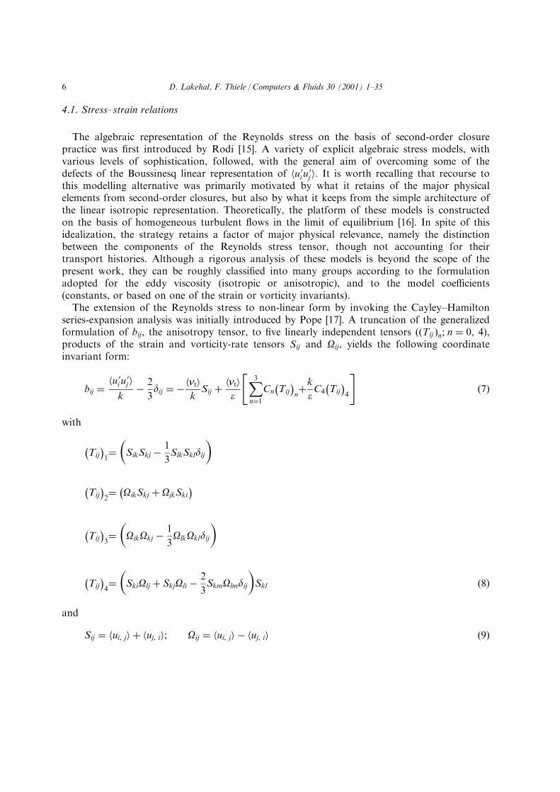
4.1. Stress±strain relations

The algebraic representation of the Reynolds stress on the basis of second-order closurepractice was ®rst introduced by Rodi [15]. A variety of explicit algebraic stress models, withvarious levels of sophistication, followed, with the general aim of overcoming some of thedefects of the Boussinesq linear representation of hu 0i u 0j i: It is worth recalling that recourse tothis modelling alternative was primarily motivated by what it retains of the major physicalelements from second-order closures, but also by what it keeps from the simple architecture ofthe linear isotropic representation. Theoretically, the platform of these models is constructedon the basis of homogeneous turbulent ¯ows in the limit of equilibrium [16]. In spite of thisidealization, the strategy retains a factor of major physical relevance, namely the distinctionbetween the components of the Reynolds stress tensor, though not accounting for theirtransport histories. Although a rigorous analysis of these models is beyond the scope of thepresent work, they can be roughly classi®ed into many groups according to the formulationadopted for the eddy viscosity (isotropic or anisotropic), and to the model coe�cients(constants, or based on one of the strain or vorticity invariants).The extension of the Reynolds stress to non-linear form by invoking the Cayley±Hamilton

series-expansion analysis was initially introduced by Pope [17]. A truncation of the generalizedformulation of bij, the anisotropy tensor, to ®ve linearly independent tensors ��Tij �n; n � 0, 4�,products of the strain and vorticity-rate tensors Sij and Oij, yields the following coordinateinvariant form:

bij �hu 0i u 0j ikÿ 2

3dij � ÿhnti

kSij � hnti

e

"X3n�1

Cn

ÿTij

�n�keC4

ÿTij

�4

#�7�

with

ÿTij

�1��SikSkj ÿ 1

3SlkSkldij

�ÿTij

�2� ÿOikSkj � OjkSki

�ÿTij

�3��OikOkj ÿ 1

3OlkOkldij

�

ÿTij

�4��SkiOlj � SkjOli ÿ 2

3SkmOlmdij

�Skl �8�

and

Sij � hui, ji � huj, ii; Oij � hui, ji ÿ huj, ii �9�


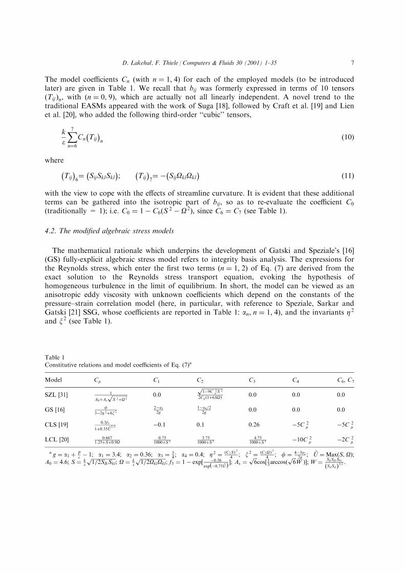
The model coe�cients Cn (with n � 1, 4� for each of the employed models (to be introducedlater) are given in Table 1. We recall that bij was formerly expressed in terms of 10 tensors�Tij �n, with �n � 0, 9), which are actually not all linearly independent. A novel trend to thetraditional EASMs appeared with the work of Suga [18], followed by Craft et al. [19] and Lienet al. [20], who added the following third-order ``cubic'' tensors,

k

e

X7n�6

Cn

ÿTij

�n

�10�

whereÿTij

�6� ÿSijSklSkl

�;

ÿTij

�7� ÿÿSijOklOkl

� �11�

with the view to cope with the e�ects of streamline curvature. It is evident that these additionalterms can be gathered into the isotropic part of bij, so as to re-evaluate the coe�cient C0

(traditionally = 1); i.e. C0 � 1ÿ C6�S 2 ÿ O2�, since C6 � C7 (see Table 1).

4.2. The modi®ed algebraic stress models

The mathematical rationale which underpins the development of Gatski and Speziale's [16](GS) fully-explicit algebraic stress model refers to integrity basis analysis. The expressions forthe Reynolds stress, which enter the ®rst two terms �n � 1, 2� of Eq. (7) are derived from theexact solution to the Reynolds stress transport equation, evoking the hypothesis ofhomogeneous turbulence in the limit of equilibrium. In short, the model can be viewed as ananisotropic eddy viscosity with unknown coe�cients which depend on the constants of thepressure±strain correlation model (here, in particular, with reference to Speziale, Sarkar andGatski [21] SSG, whose coe�cients are reported in Table 1: an, n � 1, 4), and the invariants Z2

and x2 (see Table 1).

Table 1Constitutive relations and model coe�cients of Eq. (7)a

Model Cm C1 C2 C3 C4 C6, C7

SZL [31] 1

A0�As

��S 2�O 2p 0.0

��1ÿ9C 2

m S2

p2Cm�1�6SO� 0.0 0.0 0.0

GS [16] f3ÿ2Z 2�6x 2

2ÿa32g

1ÿa4=22g 0.0 0.0 0.0

CLS [19] 0:3f3

1�0:35 ~U3=2 ÿ0.1 0.1 0.26 ÿ5C 2

m ÿ5C 2m

LCL [20] 0:6671:25�S�0:9O

0:751000�S 3

3:751000�S 3

4:751000�S 3 ÿ10C 2

m ÿ2C 2m

a g � a1 � Pe ÿ 1; a1 � 3:4; a2 � 0:36; a3 � 5

4 ; a4 � 0:4; Z 2 � �C1S� 24 ; x 2 � �C2O� 2

4 ; f � 4ÿ3a22g ; ~U � Max�S, O�;

A0 � 4:6; S � ke

��1=2SlkSkl

p; O � k

e

��1=2OklOkl

p; f3 � 1ÿ exp� ÿ0:36

exp�ÿ0:75 ~U� �; As ��6p

cos� 13arccos� ��6p

W ��;W � SijSjkSki

�SijSij �3=2 .


The constraint of ``weak equilibrium'' is, however, signi®cant in that the model is not ofpractical utility away from the equilibrium limit. Yet, since conventional two-equation modelsare nothing more than particular cases of the non-linear expression for the Reynolds stress,this assumption would, in principle, compromise their application to complex turbulent ¯ows.Nonetheless, Gatski and Speziale [16] reinforced this constraint by treating the production-to-dissipation ratio �Pk=e), where

Pk � ÿhu 0i u 0j ihui, ji � ÿkbijSij, �12�

encompassed in the expressions for C1 and C2 in Table 1, through the equilibrium solution forhomogeneous turbulence. This solution, which has been initially adopted for the SSGpressure±strain model [21], omits to represent the transport e�ects in the k- and e-equations,and yields the equilibrium value Pk=e � �Ce2ÿ 1�=�Ce1ÿ 1�11:89 (i.e. g � 0:233 in Table 1). Ine�ect, such an alternative helps alleviate the singularities of the e�ective viscosity which canarise when Pk=e is treated implicitly [22]. Later, however, the necessity to account for thechanges in the production-to-dissipation-rate ratio Pk=e was fully acknowledged [23,24],because, its equilibrium value drives the model to inconsistency when used away fromequilibrium.As a remedy, Grimaji [23] has developed a fully-explicit, self-consistent variant of the GS

model, by solving the cubic equation for Pk=e arising in the context of the selected pressure±strain model [23]. The resulting solution for Pk=e is unfortunately too cumbersome to be easilyimplemented in existing codes. However, this achievement yielded a new model variant which,in the case of irrotational straining, i.e. x10, departs signi®cantly from the regularized modelin that Cm decreases with increasing Z: Recently, Jongen and Gatski [24] have extended thesame GS model through a new approach for characterizing the equilibrium states of theReynolds stress anisotropy in homogeneous turbulence. Their model consists of a generalizedrelationship for Pk=e which can cover all planar homogeneous ¯ows, with and withoutrotation.Here, we aim at extending the forgoing e�ort to make the GS model applicable to a broad

range of practical ¯ows. To that end, we emphasize on the following two points, thoughalways in the context of a mild departure from equilibrium: (i) the development of ageneralized relation for Pk=e, which can reasonably mimic both Grimaji's [23] and Jongen andGatski's [24] models, and (ii) the formulation of a more accurate regularization procedure. Thenew calibrated relation for Pk=e will serve to determine the coe�cients C1 and C2, while itmust recover, at least, the established equilibrium values for both the logarithmic region in aturbulent boundary layer, and the homogeneous shear ¯ow. Based on the characteristics ofboth type of ¯ows, and owing to the property limS41Pk=e0S [24], the following formulationfor the production-to-dissipation ratio is proposed:

Pk

e� S 2

4:8� 1:3max�S, O� �13�

where S and O are given in Table 1. It can be easily seen that the proposed relation meets therequirement of the equilibrium state Pk=e11 for the logarithmic region in channel ¯ow, where,


by reference to Laufer's [25] data, S � 3:1: The calibration of Eq. (13) for homogeneous shear¯ow follows, however, the scale expansion theory for the Reynolds stress by reference toSpeziale and Mac Giolla Mhuiris [26]. The starting point consists in using the ``conventional''isotropic closure for the deviatoric part of the Reynolds stress in Eq. (7), i.e. htiji �ÿCm�k2=e�Sij: The dimensionless variable k� � k=k0 is then introduced, where k0 refers to theinitial turbulent kinetic energy. In so far as the case of homogeneous shear ¯ow nulli®es r 2kand r 2e in their transport equations, the deviatoric part of Eq. (7) and the dissipationequation take the following simple forms:

dk�

dt�� k�

ÿCmSÿ 1=S

�,

dS

dt�� ÿCm�Ce1 ÿ 1�S 2 � �Ce2 ÿ 1�, �14�

where t� � S � t: Setting now dS=dt � 0, we obtain the single point of the above equation

S0 ��Ce2 ÿ 1�=Cm�Ce1 ÿ 1��1=2, �15�

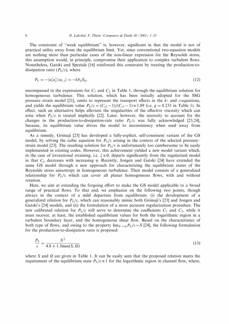
which, in the context of the GS model �Ce1 � 1:44, Ce2 � 1:83, and the equilibrium value ofCm10:094 for shear ¯ow is invoked) converges towards S0 � 4:48: This single value permitsthe equilibrium state to be correctly recovered through Pk=e�S0� � 1:89: In Fig. 1, relation (13)

Fig. 1. Locus of solution points for Pk=e as a function of S � O:


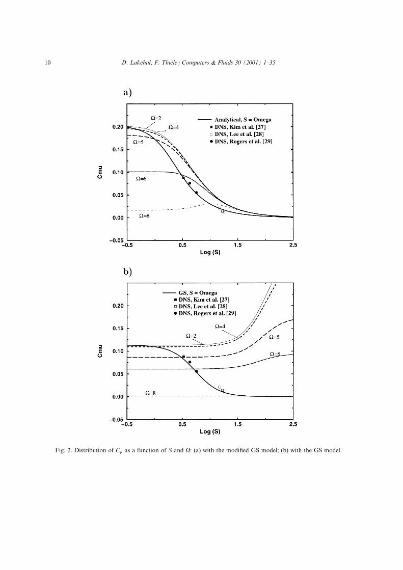
Fig. 2. Distribution of Cm as a function of S and O: (a) with the modi®ed GS model; (b) with the GS model.


is illustrated and clearly shown to recover the self-consistent models of Grimaji [23] andJongen and Gatski [24] for weak departures from equilibrium �S < 5). While it is a simplematter to show that making use of Eq. (13) does not a�ect the exponential growth of k�Aelt

�

�l refers to the rate of growth [26]), this relationship returns, however, a Cm distribution(Fig. 2a) that deviates signi®cantly from that displayed in Fig. 2b Ð results are compared withvarious DNS data, i.e. [27±29]. As shown in Fig. 2a, the result is, in fact, very similar to thatof the self-consistent model of Grimaji [23]. It should be noted that the result shown in thelatter ®gure con®rms the note of warning constantly evoked by Speziale [22] with regard to therepercussions that might follow from ®xing Pk=e: As a ¯agrant example, the GS model isunlikely to predict an impinging ¯ow because Cm has the potential to grow and thereby todrastically overestimate the eddy viscosity in Eq. (7). This can lead to the prediction of non-physical (negative) normal stress components, and thereby violate the realizability principle.It is anyway recognized [22] that, in highly-strained ¯ows, Z� 1, which nulli®es the validity

of the regularization procedure developed by Gatski and Speziale [16], resorting to a ®rst-orderPadeÂ approximation for Z2; i.e. Z21Z2

�1� Z2: This latter practice was simply abandoned in

the present work for a more elaborate formulation which invokes an approximation that isaccurate to the fourth order of Z, though di�erent from those reported recently by Speziale[22]. It takes the following form:

Z41 Z4

1� Z4; or Z21 Z2ÿ

1� Z4�1=2 �16�

and gives rise to

Cm � fÿ1� Z4

�3� Z4

ÿ1� 6x2

�ÿ 2Z2 � 6x2

�17�

This systematic regularization represents so far an excellent approximation to the original Cm �f=�3ÿ 2Z2 � 6x2� for turbulent ¯ows near equilibrium �Z and x < 1), and a much betteralternative to the ®rst-order one for ¯ows that are near equilibrium. Moreover, the expressionin Eq. (14) is regular for all values of Z and x, and has the correct asymptotic behaviour ofCm=f11=Z2 for Z� 1:Finally, to close this description, the extension of the corrected model to low-Re conditions

is achieved here by invoking a similar model-function fm to that of the one-equation model ofNorris and Reynolds [30], and adopts Jones and Launder's [14] damping of the destruction ofdissipation.The constitutive relation applied to yield the algebraic Reynolds stress model of Shih, Zhu

and Lumley [31] (SZL) was obtained using the invariance theory in continuum mechanics,while invoking the constraints based on rapid distortion theory and turbulence realizability.The model was deliberately truncated by the authors to its tensorial quadratic form. In thepresent situation, however, the model was used in its linear form �Cn � 0, n > 1� as analternative (rather than employing ad-hoc methods), to reduce the excessive rate of turbulenceproduction Pk that can be generated by conventional models at ¯ow impingement throughPk � CmeS 2: In this type of closure, the normal stresses determined through hu 0i u 0i i � 2k=3ÿ


Cmk2=eSii are not distinct, and may become negative for large positive strain rate Sii, which

then violates the realizability principle. It clearly arises that, in absence of high-order, non-linear stress±strain products forming bij, physical consistency requires special treatments foralleviating such a shortcoming, namely by imposing a constraint exclusively on Cm: Now,because the original model was found to return very high Cm values for simple homogeneous¯ows, the following correction was adopted as a remedy.3

Cm � 1

A0 � As

��S 2 � O2

p ; with A0 � 10:2ÿ 5:5tanh�0:55S� �18�

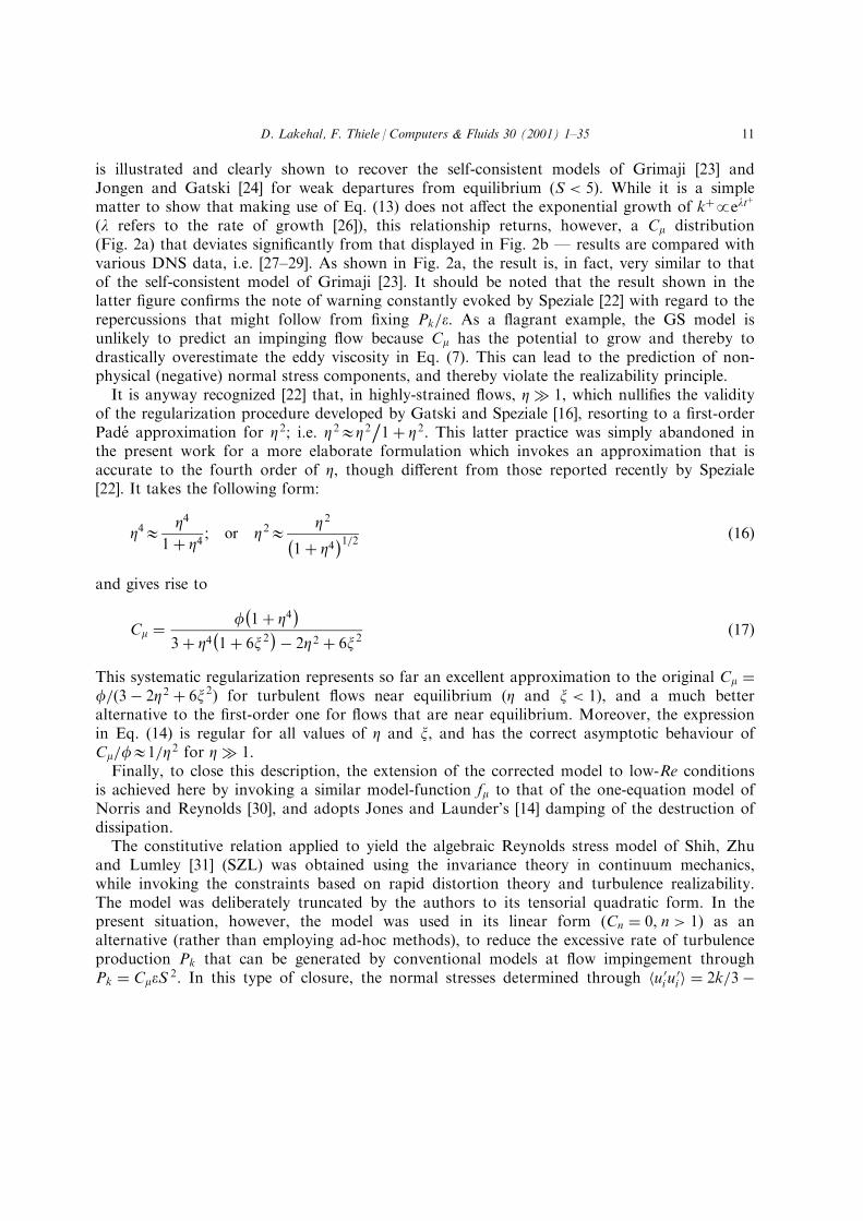
which di�ers from its original version in the way the coe�cient A0 is modelled, rather thanbeing assigned a value falling within the interval 4:0 < A0 < 6:5 [31]. The coe�cient As isde®ned in Table 1. As is to be expected, the behaviour of the modi®ed expression for Cm,illustrated in Fig. 3, departs signi®cantly from the one proposed originally.The Low-Re model of Abe et al. [32] (hereinafter referred to as AKN), which introduces the

Kolmogorov velocity scale ue � �ne�1=4 instead of the velocity scale k1=2, is employed for thenear-wall direct integration. The closure constants are assigned the non-standard valuesproposed by them, i.e C1 � 1:5, C2 � 1:9, and sk � se � 1:4: The boundary conditionsemployed for this model consist of the no-slip condition on the wall surface, k is set equal tozero, while the strict boundary condition for e, i.e. ew� 2n�@ 2=@n2�, is approximated using the

Fig. 3. Distribution of Cm as a function of S� O, obtained with the modi®ed SZL model.

3 This could also have been achieved by specifying an upper bound for Cm:


relation ejwall � 2nk=y2n : To avoid numerical instabilities, this treatment has been applied at the

®rst grid-nodes neighbouring the wall, rather than on the wall itself. The combination of thesetwo approaches which consists in replacing Cm � 0:09 in the AKN model by Eq. (18) ishereafter referred to as SZL + AKN.

4.3. The selected algebraic stress models

The EASM of Lien, Chen and Leschziner [20] (LCL) adopts the Shih et al. [31] concept,which consists in sensitizing both the eddy-viscosity and the coe�cients Cn to the straininvariant S de®ned in Table 1. In addition, the revised model claims to cope with e�ects ofstreamline curvature by including the cubic terms proposed by Suga [18]. The eddy viscosity isdamped using a similar function to the Norris and Reynolds' [30] one-equation model, whilefe2 is introduced with reference to the Jones and Launder [14] prescription. The closureconstants are assigned the standards values [14].In the EASM of Craft, Launder and Suga [19] (CLS), the constitutive relations linking the

stresses to the velocity gradients integrate the cubic terms with reference to Suga's [18] modelas well. Originally, the model was proposed to remedy the spurious normal strain-inducedproduction of turbulence resulting from the conventional isotropic concept. The approachfollows the Jones and Launder [14] model in regard to the model functions of the e-equation.

4.4. The proposed zonal Reynolds stress model

It is now recognized that the di�culties encountered in employing second-order closures aredue to their cumbersome structure rather than to the computational costs involved in solvingthe additional di�erential equations for individual turbulent stresses. It is also argued that theirdirect integration to solid walls using no-slip conditions for velocity is, to date, not viable andconstitutes an additional numerical complexity. This might partially explain, to the bestknowledge of the authors, that there exists no single, successful attempt reported forcomputing vortex-shedding ¯ows with the aid of a pure RSM in low-Re conditions since thework of Franke and Rodi [6]. Although the results of combining the Launder, Reece and Rodi[33] model (LRR) with a linear, near-wall, one-equation model by these authors were betterthan most of the previous attempts, there still exists an uncertainty with regard to the couplingof the explicitly-computed Reynolds stress components to the modelled ones. One approach tohelp alleviate such di�culties is proposed here and consists in linking dynamically (without®xed grid-layers) an outer RSM to a near-wall, one-equation, non-linear model in which theturbulence stresses are determined from stress±strain relationships (Eq. (7)). This ensuressmooth matching between the zones and, ideally, the strong near-wall anisotropy of the stressescan then be captured.In the one-equation turbulence model to be employed in the near-wall region, the eddy

viscosity is made proportional to a velocity scale �k1=2� and a length scale �lm). The distributionof �lm� is prescribed algebraically, while the velocity scale is determined by solving the transportequation for (k ), together with the mean ¯ow equations. The dissipation rate �e� appearing as asink term in the k-equation is related to k itself, and a dissipation length scale le which is also


prescribed algebraically. It should be mentioned that in the viscous sublayer lm and le deviatefrom the linear dependence on distance from the wall in order to account both for thedamping of nt and the limiting behaviour of e at the wall. The one-equation turbulence modelemployed here is due to Wolfshtein [34] and reads:

nt � Cmk1=2lm; lm � Cl yn

�1ÿ exp

ÿÿ Ry=Am��|��{z��}

fm

�19�

e � k3=2=le; le � Clyn�1ÿ exp

ÿÿ Ry=Ae�� 20�

The exponential reduction �fm between brackets) of the length scale lm involves the near-wallReynolds number Ry � k1=2yn=n: The constant Cl is set equal to kC ÿ3=4m to conform to thelogarithmic law of the wall �k is the von KaÂ rmaÂ n constant), while Ae � 2Cl is set in order toreproduce the asymptotic behaviour of ejwall � 2nk=y2

n : The empirical constant appearing in thedamping function fm is assigned the standard value Am � 70 [34].The phase-averaged, Reynolds-stress transport equations can be expressed in the following

compact form

@htiji@t� @hukihtiji

@xk� hDm

iji � hDTiji � hPiji � hFiji ÿ heiji �21�

where production and molecular di�usion are designated by the terms hPiji and hDmiji,

respectively. Both the pressure±strain correlation hFiji and turbulent di�usion hDTiji need to be

modelled. In the present case, hDTiji is modelled using the generalized gradient di�usion

approach of Daly and Harlow [35], and incorporates the damping function fm appearing in Eq.(19):

hDTiji �

@

@xk

�ÿrCsfmhtkli

�@htiji@xl

��22�

Modelling of hFiji follows Gibson and Launder's [36] proposal for the wall re¯ection terms andemploys the coe�cients of the IP pressure±strain model proposed by Gibson and Younis [37](GY), i.e. a1 � 3:0, a2 � 0:8, a3 � 1:2, a4 � 1:2, and g � 4:0: The transport equations for theReynolds stress tensor are solved together with a transport equation solving the turbulenceenergy dissipation rate e: Within the viscous sublayer, the Reynolds stresses appearing in themomentum equations are determined through stress±strain relations, retaining, as in [16], termsup to the quadratic products of the strain and vorticity tensors in Eq. (7), i.e. Cn�Tij �n � 0 forn � 3, 7: The model coe�cients C1 and C2 are determined following Gatski and Speziale's [16]paths in the derivation of their SSG-based EASM; they read C1 � 0:1, C2 � 0:05 and f � 0:2(see Table 2 for Cn � f�an�). It should be noted, however, that Cm is assigned here its standardvalue 0.09 in order to match the constant Cl � kC ÿ3=4m at the edge of the viscosity-a�ectedlayer.It is relevant to note that various other well known pressure±strain models were tested, but

without success, including that of Speziale, Sarkar and Gatski [21]. The outer RSM and the


non-linear, near-wall model are matched dynamically at a location where viscous e�ectsbecome negligible, i.e. where the near-wall Reynolds number Ry � k1=2yn=n � 80; this choice ismade on the basis of DNS data from channel and boundary layer simulations, as explained byLakehal and Rodi [38]. The proposed dynamic zonal strategy di�ers from classical two-layerapproaches in which two sub-domains are distinct. Here, both the one-equation model and theRSM are solved separately, everywhere in the domain, then both solutions are compared: in¯ow regions where Ry < 80, the RSM solutions are clipped and replaced by those obtained bythe one-equation model.

5. Computational methodology

5.1. Numerical procedure

The two-dimensional version of the Navier±Stokes equations solver ELAN was employedfor the computations. The algorithm consists of a semi-structured, multi-block, multi-grid®nite-volume method. The structure of the code is based on the strong conservation formwithin general, body-®tted coordinates, and employs a fully co-located storage arrangement forall quantities. In this, di�usion terms are approximated using second-order central di�erences,whereas advective ¯uxes can be approximated using various high-order bounded (monotonic)schemes, the latter applied in scalar form by means of a deferred-correction procedure. Thepresent computations were performed employing the well known QUICK scheme to allvariables, the truncation error of which is proportional to the third power of grid size andfourth-order derivative of velocity. The odd±even decoupling problem of the cell-centredscheme is suppressed with a fourth-order, arti®cial-dissipation apparent pressure term in thecontinuity equation. The solution is iterated to convergence using a compressible (all-speed)pressure-correction approach. The temporal discretization consists of a second-order, back-stepscheme for all variables.

5.2. Grids and boundary conditions

The dimensions of the computational domain were set as follows: each lateral boundary islocated at 6D from the centre line, the in¯ow and out¯ow planes being 4.5D upstream and 15Ddownstream the cylinder, respectively. Grid-independent results were obtained with a re®nedmesh consisting of 226� 156 grid points4 in the x- and y-directions. The computation domainand grid are shown in Fig. 4. Solving Accurate solution of the system was found to be closelyrelated to the grid concentration in near-wall regions, in particular, for the models in which thestress±strain model coe�cients Cn depend on the irrotational strain Z2 (or S 2), the near-wallgradient of which is very steep. The additional grid-sensitivity which was made on the ®nest

4 All the references cited in here, i.e. [5±8], have employed a coarser grid than the present one.


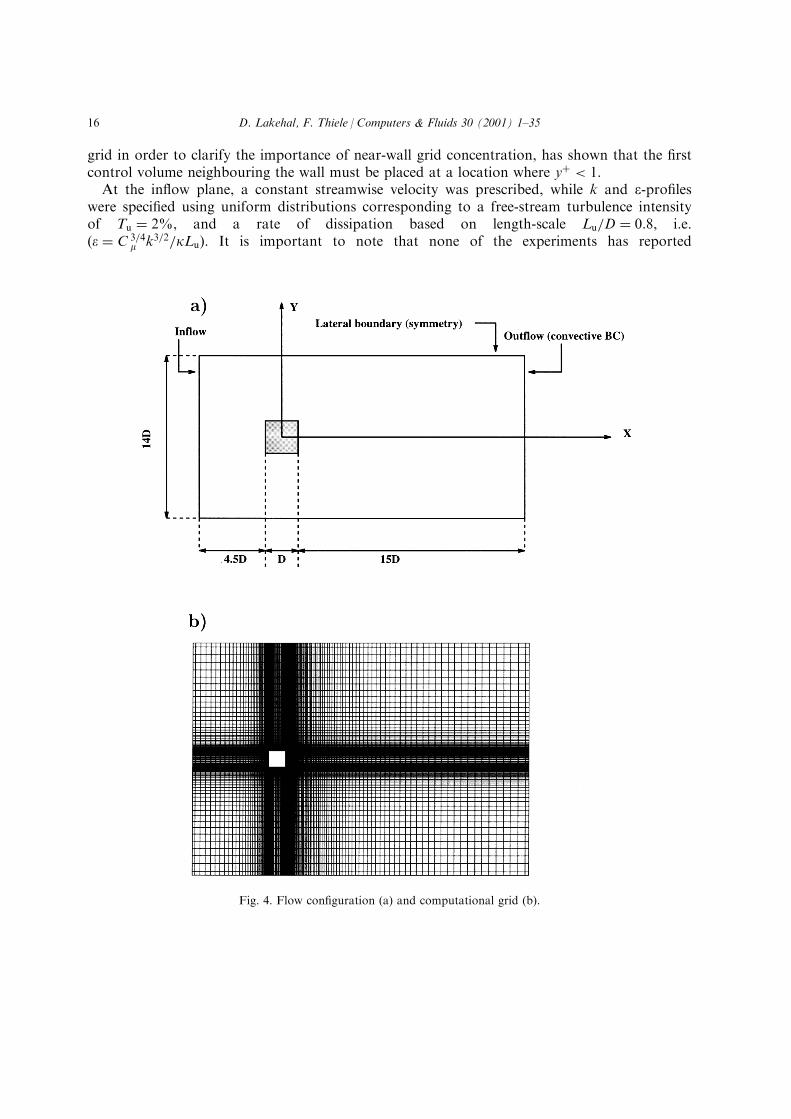
grid in order to clarify the importance of near-wall grid concentration, has shown that the ®rstcontrol volume neighbouring the wall must be placed at a location where y� < 1:At the in¯ow plane, a constant streamwise velocity was prescribed, while k and e-pro®les

were speci®ed using uniform distributions corresponding to a free-stream turbulence intensityof Tu � 2%, and a rate of dissipation based on length-scale Lu=D � 0:8, i.e.�e � C 3=4

m k3=2=kLu). It is important to note that none of the experiments has reported

Fig. 4. Flow con®guration (a) and computational grid (b).


information concerning the length-scale for this rate of turbulence intensity. The choice of sucha level of Lu=D may be questionable if one considers the laminar-turbulent transitional nature(which is reported in Lyn's et al. [3] experiment) of the ¯ow �Lu is probably much smaller).However, in a recent work investigating the implications of in¯ow conditions of turbulence (tobe submitted), the authors have found that similar results can be obtained with a linear andnon-linear low-Re model (e.g. SZL), for di�erent levels of imposed length-scale, i.e. Lu=D � 0:1and 0.8. The other reason for our choice of Lu=D is to permit a coherent comparison with theprevious investigations, and in particular, with Franke and Rodi's [6] RSM results. Non-re¯ective conditions were employed at the out¯ow cross-section for velocity components andindividual Reynolds stresses (RSM), whereas a condition of zero-gradient was imposed for allother variables. In total, 40 h CPU time on the Cray T90 vector machine at the University ofKiel, Germany, were needed to perform 30 periods; each necessitating approximately 400 time-steps of Dt � 0:02S, depending on the predicted Strouhal number. The system of equations wasiterated till the mass±¯ux residuals were reduced by three orders during each time step. Wealso note that the number of inner iterations per time step was about two orders of magnitudehigher than for the RSM computations.

6. Discussion of results

6.1. E�ects of the numerics and in¯ow conditions

The sensitivity of numerical schemes, grid dependence, time step variations, boundaryconditions, etc., were studied in two separate works (see [1,2]). Noteworthy is to recall themajor ®ndings, some of which are actually well known, such as the absolute requirement for ahigh-order discretization scheme. It was found that a minimized expansion ratio between thecross-stream grid-lines �Dxi=Dxiÿ1 < 1:1� is required for structured grids, because otherwise anyhigh-order discretization scheme would lose accuracy. However, adopting non-re¯ectiveboundary conditions rather than conventional zero-gradient ones did allow to signi®cantlyreduce the dimensions of the computational domain, in comparison with previouscontributions in which the outer boundary was extended up to 60D [8]. Employing these non-re¯ective conditions was also relevant for predicting the time to the ®rst vortex-shedding.With regard to in¯ow conditions of turbulence, the computations employing any of the low-

Re isotropic models on the basis of a length-scale Lu=D > 0:5 (i.e. nt150� n� did not succeed.This may partially explain the relative success of Bosch [5] with the standard k±e model, whoopted for nt � 10� n, in comparison with Franke and Rodi [6] who used nt � 100� n: Thisobservation is valid for low-Re model calculations as well: for instance, Kawamura andKawashima [7] have had success with nt120� n: Many other authors, such as Deng et al. [8],report however that they failed to calculate this ¯ow with a pure low-Re model, and it is notimpossible that it was simply due to their choice5 of Lu=D. This ®nding has motivated an

5 Deng et al. [8] did not report information concerning the imposed length-scale Lu=D.


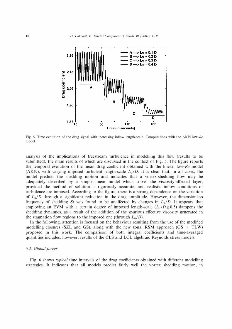
analysis of the implications of freestream turbulence in modelling this ¯ow (results to besubmitted), the main results of which are discussed in the context of Fig. 5. The ®gure reportsthe temporal evolution of the mean drag coe�cient obtained with the linear, low-Re model(AKN), with varying imposed turbulent length-scale Lu=D: It is clear that, in all cases, themodel predicts the shedding motion and indicates that a vortex-shedding ¯ow may beadequately described by a simple linear model which solves the viscosity-a�ected layer,provided the method of solution is rigorously accurate, and realistic in¯ow conditions ofturbulence are imposed. According to the ®gure, there is a strong dependence on the variationof Lu=D through a signi®cant reduction in the drag amplitude. However, the dimensionlessfrequency of shedding St was found to be una�ected by changes in Lu=D: It appears thatemploying an EVM with a certain degree of imposed length-scale �Lu=Dr0:5� dampens theshedding dynamics, as a result of the addition of the spurious e�ective viscosity generated inthe stagnation ¯ow regions to the imposed one (through Lu=D).In the following, attention is focused on the behaviour resulting from the use of the modi®ed

modelling closures (SZL and GS), along with the new zonal RSM approach (GS + TLW)proposed in this work. The comparison of both integral coe�cients and time-averagedquantities includes, however, results of the CLS and LCL algebraic Reynolds stress models.

6.2. Global forces

Fig. 6 shows typical time intervals of the drag coe�cients obtained with di�erent modellingstrategies. It indicates that all models predict fairly well the vortex shedding motion, in

Fig. 5. Time evolution of the drag signal with increasing in¯ow length-scale. Computations with the AKN low-Remodel.


particular, the modi®ed GS (the original regularized version failed; no shedding was predicted).The ®gure suggests that a clear Strouhal number can be determined from each result, and theamplitude of the main mode ~Cd strongly depends on the nature of the model. Simply, theresulting drag signal is almost regular with calculations using the linear SZL model, whilesigni®cant lower to higher frequency modulation of its amplitude appears with increasing orderof the non-linear terms of bij: This ®nding contrasts somewhat the accepted argument [6] whichstates that, by imposing two-dimensionality to the mean ¯ow, the RANS concept is supposedto yield a regular shedding motion. It is also interesting to note that the amplitude of the mainmode ~Cd delivered by the RSM model is the smallest, as con®rmed in Table 2. The same trendcan be seen on time evolutions of the lift coe�cient Cl in Fig. 7; it clearly indicates asigni®cant in¯uence of non-linear expressions of Reynolds stress on the behaviour of eachmodel, be they algebraically determined (GS and CLS) or individually calculated (GL +TLW). Again, results of the anisotropic, eddy-viscosity model SZL show regular modulation,while the strong lower to higher frequency variation is now truly established as being the resultof transcending the conventional eddy-viscosity approach. In comparison with Murakami's [10]LES data, Table 2 indicates that nearly all algebraic stress models overpredict both Cd, rms andCl, rms, while a noticeable improvement is brought about by the RSM. Most notably, thoughnot reported in Table 2, is that �Cl delivered by the RSM was equal to �Cl � ÿ0:03, revealingthereby the asymmetric shedding above and below the wake centerline, as was the case in mostof the LES reported in [11].

The particular irregularity of the shedding dynamics obtained using the RSM is intriguing.

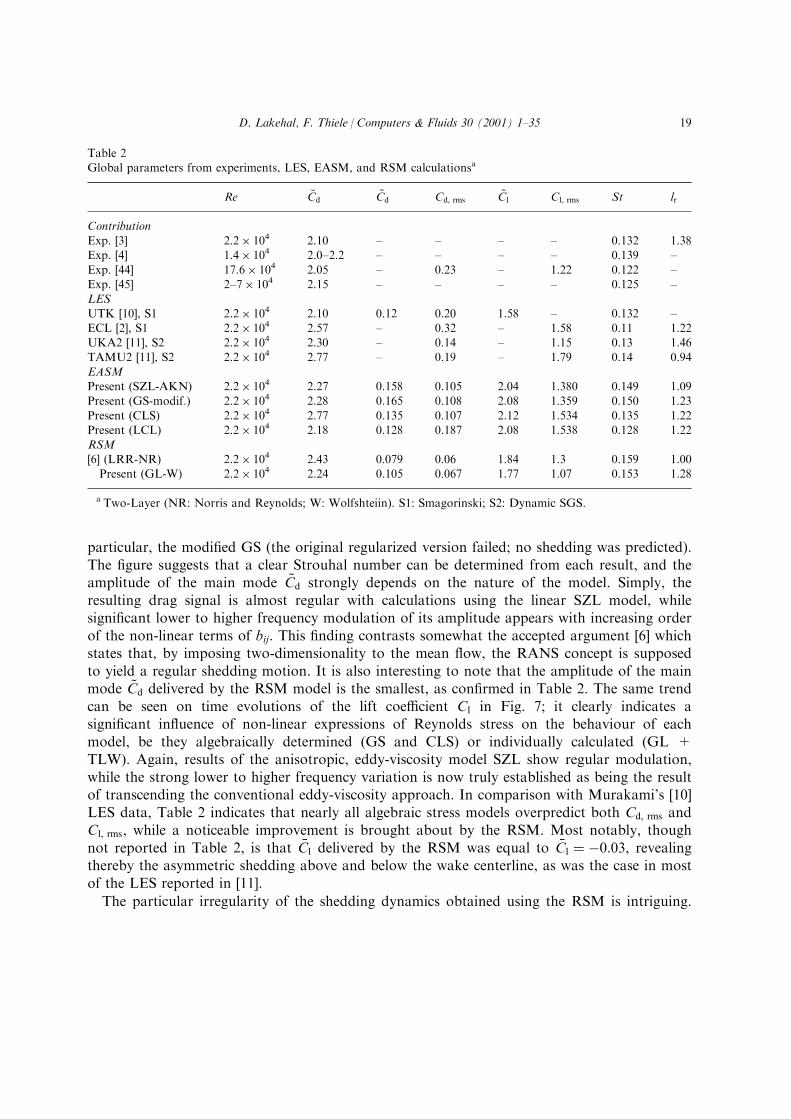
Table 2Global parameters from experiments, LES, EASM, and RSM calculationsa

Re �Cd~Cd Cd, rms

~Cl Cl, rms St lr

ContributionExp. [3] 2.2� 104 2.10 ± ± ± ± 0.132 1.38Exp. [4] 1.4� 104 2.0±2.2 ± ± ± ± 0.139 ±

Exp. [44] 17.6� 104 2.05 ± 0.23 ± 1.22 0.122 ±Exp. [45] 2±7� 104 2.15 ± ± ± ± 0.125 ±LES

UTK [10], S1 2.2� 104 2.10 0.12 0.20 1.58 ± 0.132 ±ECL [2], S1 2.2� 104 2.57 ± 0.32 ± 1.58 0.11 1.22UKA2 [11], S2 2.2� 104 2.30 ± 0.14 ± 1.15 0.13 1.46TAMU2 [11], S2 2.2� 104 2.77 ± 0.19 ± 1.79 0.14 0.94

EASMPresent (SZL-AKN) 2.2� 104 2.27 0.158 0.105 2.04 1.380 0.149 1.09Present (GS-modif.) 2.2� 104 2.28 0.165 0.108 2.08 1.359 0.150 1.23

Present (CLS) 2.2� 104 2.77 0.135 0.107 2.12 1.534 0.135 1.22Present (LCL) 2.2� 104 2.18 0.128 0.187 2.08 1.538 0.128 1.22RSM

[6] (LRR-NR) 2.2� 104 2.43 0.079 0.06 1.84 1.3 0.159 1.00Present (GL-W) 2.2� 104 2.24 0.105 0.067 1.77 1.07 0.153 1.28

a Two-Layer (NR: Norris and Reynolds; W: Wolfshteiin). S1: Smagorinski; S2: Dynamic SGS.


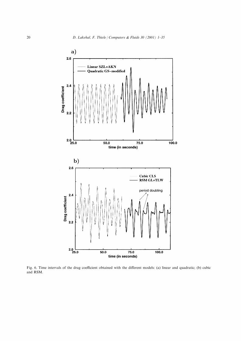
Fig. 6. Time intervals of the drag coe�cient obtained with the di�erent models: (a) linear and quadratic; (b) cubicand RSM.


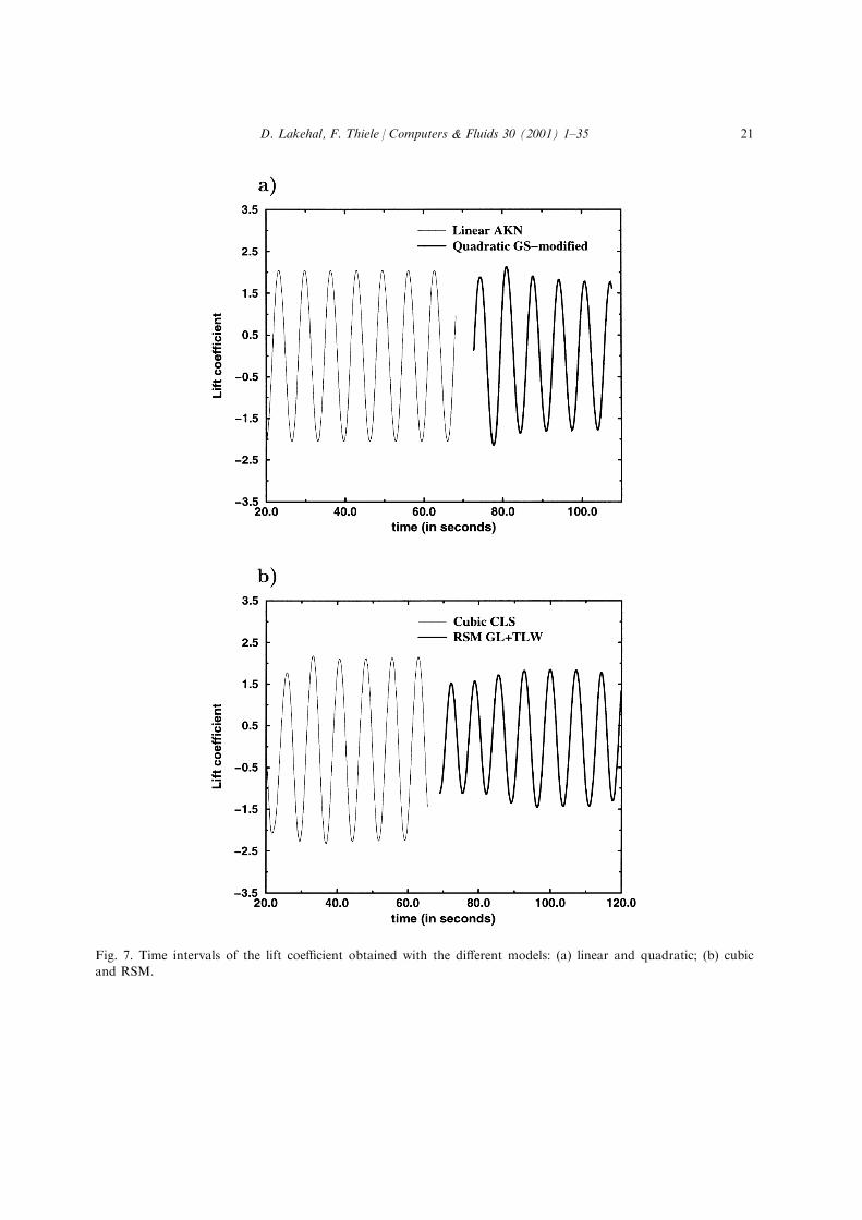
Fig. 7. Time intervals of the lift coe�cient obtained with the di�erent models: (a) linear and quadratic; (b) cubic

and RSM.


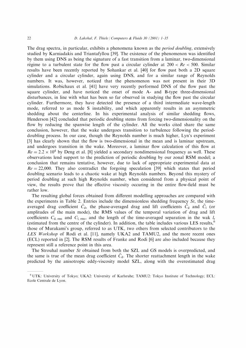
The drag spectra, in particular, exhibits a phenomena known as the period doubling, extensivelystudied by Karniadakis and Triantafyllou [39]. The existence of the phenomenon was identi®edby them using DNS as being the signature of a fast transition from a laminar, two-dimensionalreÂ gime to a turbulent state for the ¯ow past a circular cylinder at 200 < Re < 500: Similarresults have been recently reported by Sohankar et al. [40] for ¯ow past both a 2D squarecylinder and a circular cylinder, again using DNS, and for a similar range of Reynoldsnumbers. It was, however, noticed that the phenomenon was not present in their 3Dsimulations. Robichaux et al. [41] have very recently performed DNS of the ¯ow past thesquare cylinder, and have noticed the onset of mode A- and B-type three-dimensionaldisturbances, in line with what has been so far observed in studying the ¯ow past the circularcylinder. Furthermore, they have detected the presence of a third intermediate wave-lengthmode, referred to as mode S instability, and which apparently results in an asymmetricshedding about the centerline. In his experimental analysis of similar shedding ¯ows,Henderson [42] concluded that periodic doubling stems from forcing two-dimensionality on the¯ow by reducing the spanwise length of the cylinder. All the works cited share the sameconclusion, however, that the wake undergoes transition to turbulence following the period-doubling process. In our case, though the Reynolds number is much higher, Lyn's experiment[3] has clearly shown that the ¯ow is two-dimensional in the mean and is laminar upstream,and undergoes transition in the wake. Moreover, a laminar ¯ow calculation of this ¯ow atRe � 2:2� 104 by Deng et al. [8] yielded a secondary nondimensional frequency as well. Theseobservations lend support to the prediction of periodic doubling by our zonal RSM model; aconclusion that remains tentative, however, due to lack of appropriate experimental data atRe � 22,000: They also contradict the forgoing speculation [39] which states that perioddoubling scenario leads to a chaotic wake at high Reynolds numbers. Beyond this mystery ofperiod doubling at such high Reynolds number, when considered from a physical point ofview, the results prove that the e�ective viscosity occuring in the entire ¯ow-®eld must berather low.

The resulting global forces obtained from di�erent modelling approaches are compared withthe experiments in Table 2. Entries include the dimensionless shedding frequency St, the time-averaged drag coe�cient �Cd, the phase-averaged drag and lift coe�cients ~Cd and ~Cl (oramplitudes of the main mode), the RMS values of the temporal variation of drag and liftcoe�cients Cd, rms and Cl, rms, and the length of the time-averaged separation in the wak lr(estimated from the centre of the cylinder). In addition, the table includes various LES results,6

those of Murakami's group, referred to as UTK, two others from selected contributors to theLES Workshop of Rodi et al. [11], namely UKA2 and TAMU2, and the more recent ones(ECL) reported in [2]. The RSM results of Franke and Rodi [6] are also included because theyrepresent still a reference point in this area.

The Strouhal number St obtained from both the SZL and GS models is overpredicted, andthe same is true of the mean drag coe�cient �Cd: The shorter reattachment length in the wakepredicted by the anisotropic eddy-viscosity model SZL, along with the overestimated drag

6 UTK: University of Tokyo; UKA2: University of Karlsruhe; TAMU2: Tokyo Institute of Technology; ECL:Ecole Centrale de Lyon.


coe�cient, indicate an exaggerated rate of momentum exchange in this region. This is apossible result of over-suppression of turbulence production Pk in front of the cylinder due tothe modi®ed relation for Cm: Furthermore, the predicted shedding frequency exhibits anoticeable reaction to turbulence modelling using stress±strain expressions, decreasing towardsthe measured level with increasing order of strain and vorticity products of bij: Nonetheless,the algebraic Reynolds stress models give satisfactory agreement between calculation andmeasurement for �Cd, and, against all expectations, much better than the most recent LESresults. Incorporation of the Suga's [18] triple strain±strain and strain±vorticity correlations,n � 6 and 7, in both models CLS and LCL seems to bring a signi®cant improvement over thequadratic GS approach through the prediction of a better Strouhal number and dragcoe�cient. However, this picture of superiority does not extend to all other parameters, suchas the length of separation in the wake lr, which remains unchanged for both the EASMs,

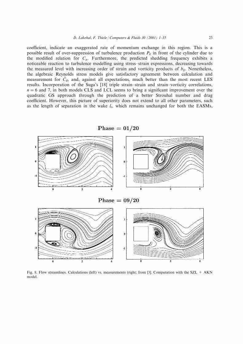
Fig. 8. Flow streamlines. Calculations (left) vs. measurements (right; from [3]. Computation with the SZL + AKNmodel.


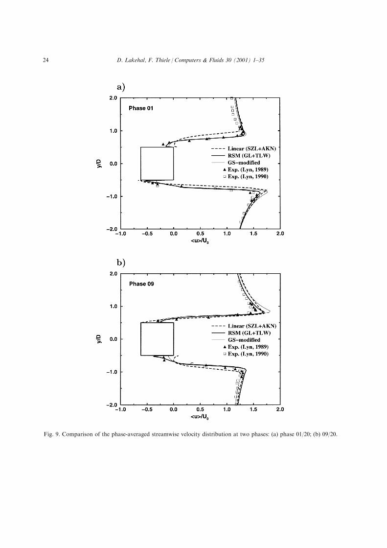
Fig. 9. Comparison of the phase-averaged streamwise velocity distribution at two phases: (a) phase 01/20; (b) 09/20.


quadratic or cubic. At this stage, it appears justi®able to reintroduce the Strouhal number Stas an appropriate indicator of e�cacy of the non-linear models, in contrast to conventionalmodels, since previous investigations of the authors (results to be submitted) have revealed Stto be much less sensitive to either the particular low-Re scheme utilized or to the imposedin¯ow conditions of turbulence.The novel zonal Reynolds stress transport model is probably the most re®ned strategy for

this particular ¯ow. Results reported in Table 2 indicate a clear superiority in predicting meandrag coe�cient �Cd and recirculation length lr, though the intensity of the wave motion,expressed through an overestimated St, is overpredicted. The present ®ndings are in fact betterthan earlier results of Franke and Rodi [6]. Because the computation details are very similar(in particular, space and time di�erencing schemes, and time step Dt), the di�erence inbehaviour stems probably from adopting the algebraic stress±strain relations in the one-equation model. In summary, the zonal RSM approach can produce much better global forcesthan selected LES (except Murakami's [10] contribution), which still display a disparatebehaviour, at least in this particular context.

6.3. Phase-averaged quantities

Comparison of the phase-averaged quantities is limited here to ¯ow streamlines Fig. 8, hui-velocity pro®les in the leeward plane of the cylinder (Fig. 9), and hvi-velocity pro®les on thecenter line of the cylinder, calculated with the modi®ed SZL and GS, and from the zonal RSMapproach, respectively. The streamlines are compared with the experimental data of Lyn et al.[3], while selected data from earlier measurements of Lyn (private communications) arecompared with the predicted hui- and hvi-velocity pro®les. The non-linear models producedvirtually identical streamlines to that of the linear SZL model, and the same is true of theRSM. Clearly, there is reasonable agreement between computations and measurements,although there is a lack of information on the structure of attached/separated shear layers onside walls of the cylinder from the measurements. Close examination of Fig. 8 suggests,however, that the simulated shedding motion is more sustained than in the experiment, whichconforms with the resulting integral parameters St and �Cd:The superiority of both the modi®ed GS model and the zonal RSM closure over the linear

SZL model is re¯ected from the distributions of hui velocity (Fig. 9), which indicate thatEASMs and RSM only are able to adequately reproduce the reverse ¯ow on both sides of thebody simultaneously; this is a major improvement in comparison with the previous results ofFranke and Rodi, including their two-layer, second-order LRR model. However, as has beenso far aknowledged that an accurate prediction of the ¯ow in this region is strongly dependenton the numerics rather than the turbulence modelling [11], establishing the superiority of onemodel over the other cannot be justi®ed in this context. It should be mentioned here that nomodel has predicted ¯ow reattachment on the side wall during the selected phases. Ensemble-averaged hvi-velocity pro®les plotted in Fig. 10 have the merit of revealing the strength of theshedding process in the wake. Indeed, far downstream of the cylinder (at x=D > 4), all thecalculations predict the lateral ensemble-averaged velocity much higher than in experiment.


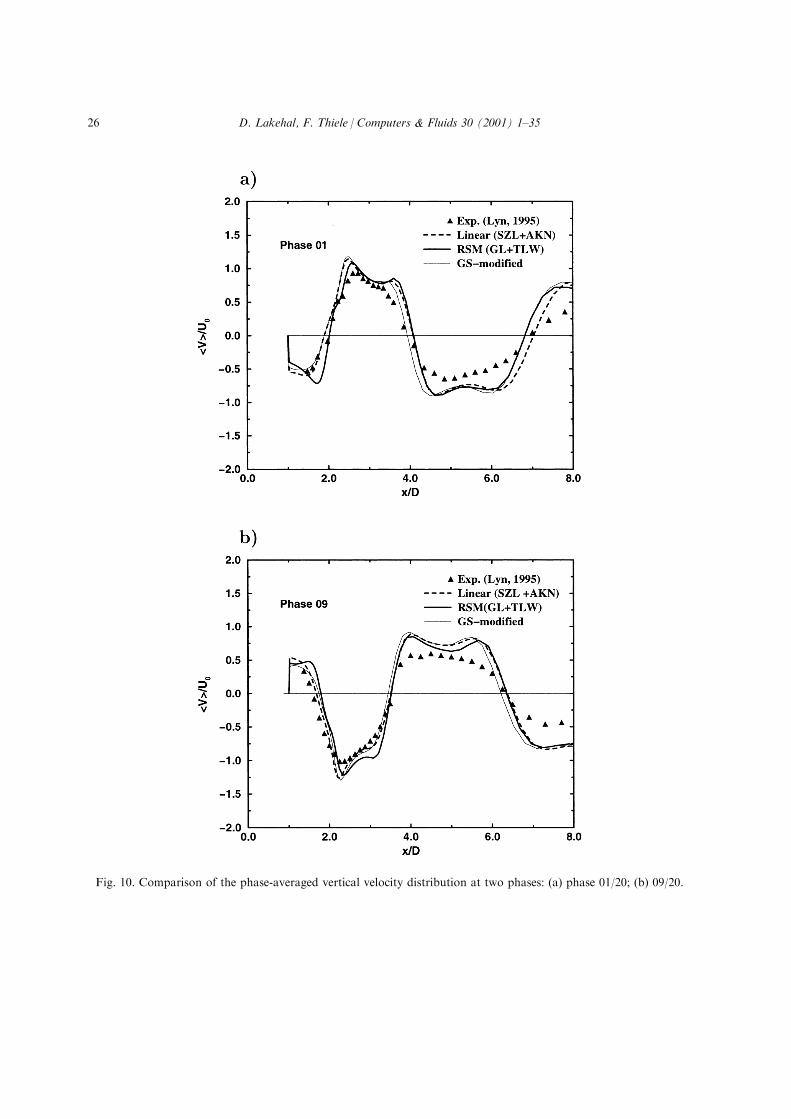
Fig. 10. Comparison of the phase-averaged vertical velocity distribution at two phases: (a) phase 01/20; (b) 09/20.


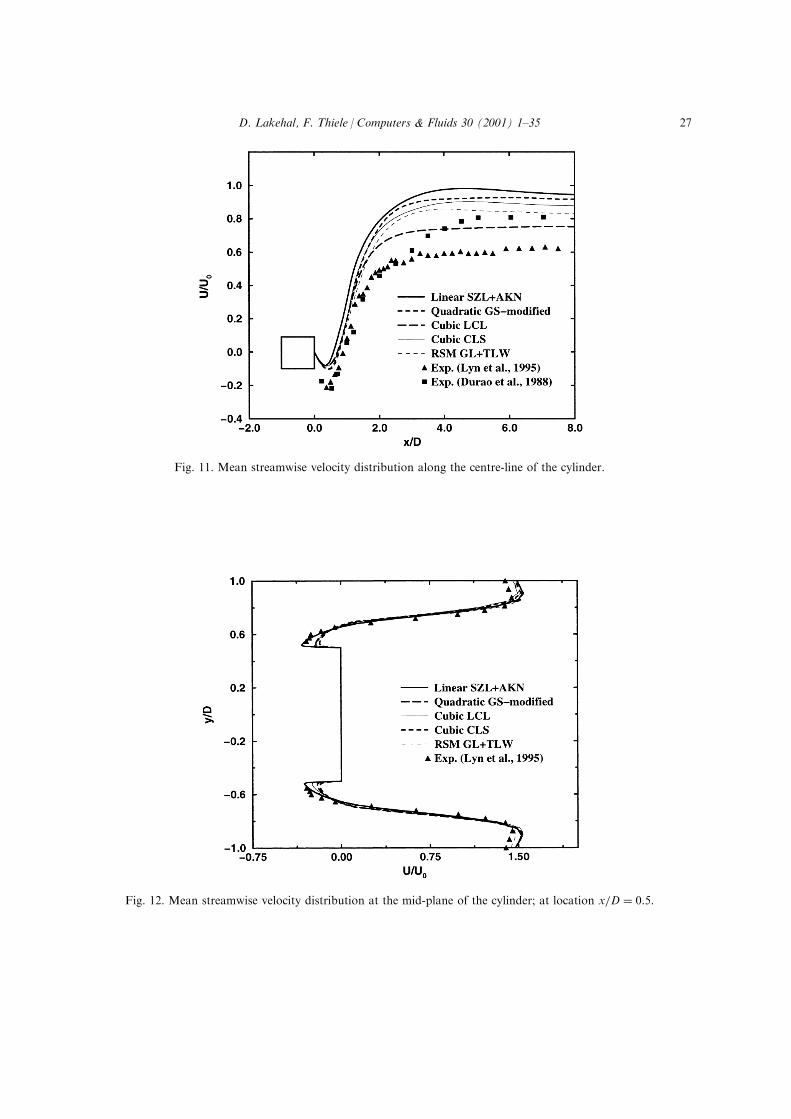
Fig. 11. Mean streamwise velocity distribution along the centre-line of the cylinder.

Fig. 12. Mean streamwise velocity distribution at the mid-plane of the cylinder; at location x=D � 0:5:


This shows the excessive rate of momentum exchange in the wake a�ects not only the sheddingfrequency and drag coe�cient, but also the vertical velocity component.

6.4. Time-averaged quantities

Time-averaged streamwise velocities �U along the centerline of the cylinder are compared fordi�erent cases in Fig. 11. The information concerning the length of the recirculation zonealready discussed is con®rmed: lr is underestimated by the SZL model, while the non-linearmodels and the zonal RSM model show clear improvement. None of the models is able tocorrectly predict the back¯ow which is always underestimated. This result was formerlyattributed by Deng et al. [8] to the smaller computational domain, whereas the recent analysisof freestream turbulence e�ects by the authors, has revealed that a high level of imposede�ective viscosity signi®cantly in¯uences the back¯ow too. However, apart from the linear SZLmodel which, exhibits a very fast approach to the free-stream velocity due to an intensiveshedding motion in body wake, there are large variations between all the other models. In allsituations, ¯ow recovery to the non-perturbed state is prematurely predicted, though less so forthe cubic LCL and the zonal RSM, at least if the comparisons are limited with Durao' et al.[4] measurements. This behaviour arises as a common picture of two-dimensional RANS, ashas been revealed by many authors (at least these cited here). Following Williamson [43]indeed, a nominally two-dimensional motion of the coherent structures engenders a transfer ofkinetic energy towards the third direction. This feature cannot be captured by any sort of two-dimensional calculation.

Fig. 13. Mean turbulent kinetic energy distribution on the centre-line of the cylinder.


Fig. 12 presents a close-up of the distribution of mean velocity �U at the mid-plane of thecylinder. The mean ¯ow ®eld in this region is particularly well described by all models, andcomplete agreement with experiment is nearly achieved. This is the best guarantee of adequategrid resolution on the cylinder side-walls. The superior behaviour of the SZL model regardingprediction of the reverse ¯ow very close to the wall is, as mentioned earlier, a possibleconsequence of over-suppression of turbulence production Pk at ¯ow stagnation. Since thislocation is entirely dominated by shear, the impact of the non-linear terms in bij is minor, sothat the e�ciency of the model can be judged entirely with respect to Cm: Such an observationwas already noted by Lakehal and Rodi [38] when the Kato and Launder Pk-suppressionmeasure [9] was employed for the ¯ow past a 3D mounted-cube. As was to be expected, onlymarginal deviations between the EASMs and RSM results can be noticed in this narrow ¯owregion adjacent to the wall.

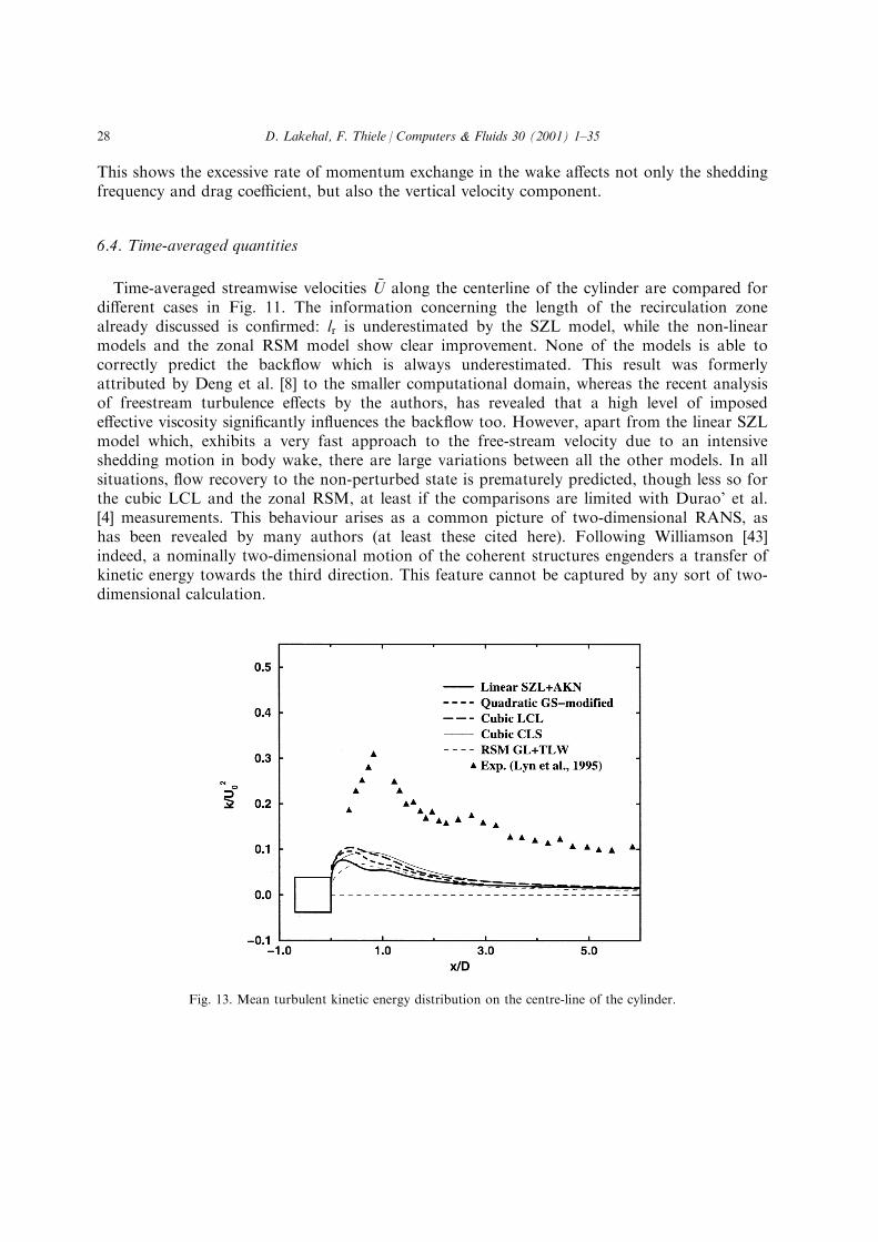
The results of the mean turbulent kinetic-energy contribution to the total ¯uctuating one arecompared with the experimental data in Fig. 13. Overall, the level of calculated turbulentkinetic energy is much too small, though a relative improvement (about 30% is now visiblethrough the incorporation of the cubic terms due to Suga into the LCL and CLS models, incomparison with the linear and quadratic closures, SZL and GS-modi®ed. This result is notsurprising in view of what was originally expected from the additive cubic correlations of Sij

and Oij, namely to enhance sensitivity to streamline curvature. More precisely, the two groupsC6�Tij �6 and C7�Tij �7 constitute the unique linkage between anisotropy and shear stress throughthe quantity �S 2 ÿ O2�, which is negative within the curved shear-layers bordering the KaÂ rmaÂ nstreet. Lien et al. [20] report about this feature in the wake of a ¯ow past a 2D hill. Such alinkage may increase the e�ective viscosity through the corrected coe�cient C0, as explainedpreviously, and explains the scatter in the pro®les of k. However, there is really no clearindication on how important the sensitivity to streamline curvature in the wake ¯ow region isexactly represented by these additive groups in �bij �:The enhanced level of turbulent kinetic energy in the wake by the cubic models might ®nd

its roots in the low-frequency ¯uctuations exhibited by the drag signals; a statement which is inline with the observations of Lyn et al. [3]. On the other hand, Williamson's [43] review onvortex dynamics in the cylinder wake states that the three-dimensionality of the coherentstructures generates a secondary ¯ow instability which, in turn, supplies the three-dimensionalstochastic ¯uctuating ®eld. In other words, a nominally two-dimensional vortex motion in thecylinder wake hides an intensive three-dimensionality of the non-coherent ¯uctuations. Apurely second-order closure, together with a near-wall one-equation EASM, also fails toreproduce the rate of turbulent kinetic energy. Since this weakness is now acknowledged to bethe logical consequence of forcing two-dimensionality on the ¯ow, it is not evident to allowone to question the employed modelling strategies as a matter of priority.

Fig. 14a compares ktot, the total ¯uctuating energy (periodic and turbulent) withmeasurements. The ®gure shows that, overall, reasonable agreement is achieved, though thepeak is occasionally underpredicted. Signi®cant departures of the values both from each otherand from the data of Lyn are revealed in the far wake region, except from the LCL cubicmodel. Note, in addition, that nearly all models which overpredict ktot in the energy-decayregion systematically exaggerate both the mean drag coe�cient and Strouhal number (see


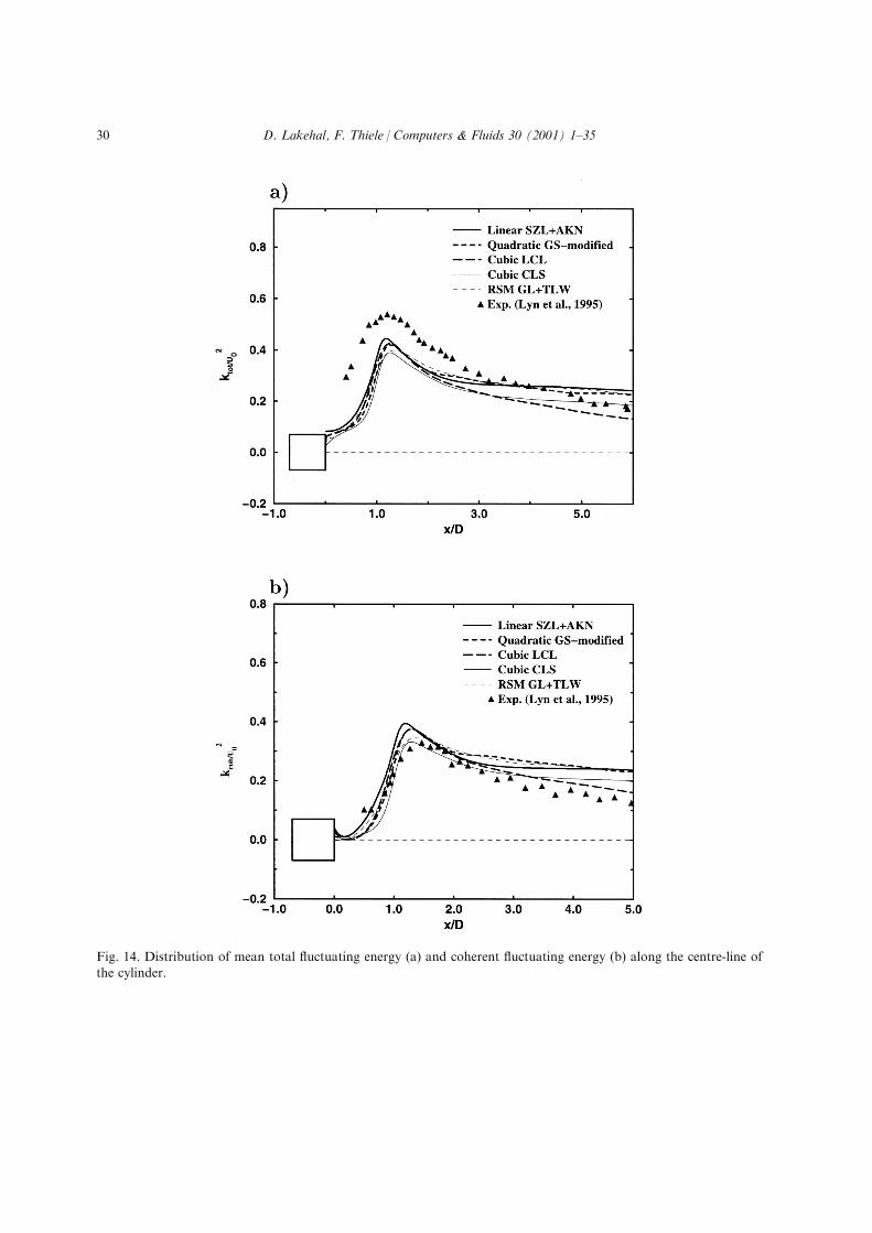
Fig. 14. Distribution of mean total ¯uctuating energy (a) and coherent ¯uctuating energy (b) along the centre-line of

the cylinder.


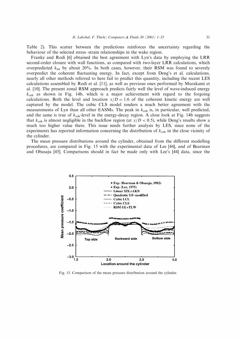
Table 2). This scatter between the predictions reinforces the uncertainty regarding thebehaviour of the selected stress±strain relationships in the wake region.Franke and Rodi [6] obtained the best agreement with Lyn's data by employing the LRR

second-order closure with wall functions, as compared with two-layer LRR calculations, whichoverpredicted ktot by about 20%. In both cases, however, their RSM was found to severelyoverpredict the coherent ¯uctuating energy. In fact, except from Deng's et al. calculations,nearly all other methods referred to here fail to predict this quantity, including the recent LEScalculations assembled by Rodi et al. [11], as well as previous ones performed by Murakami etal. [10]. The present zonal RSM approach predicts fairly well the level of wave-induced energykcoh as shown in Fig. 14b, which is a major achievement with regard to the forgoingcalculations. Both the level and location x=D � 1:6 of the coherent kinetic energy are wellcaptured by the model. The cubic CLS model renders a much better agreement with themeasurements of Lyn than all other EASMs. The peak in kcoh is, in particular, well predicted,and the same is true of kcoh-level in the energy-decay region. A close look at Fig. 14b suggeststhat kcoh is almost negligible in the back¯ow region (at x=D < 0:5), while Deng's results show amuch too higher value there. This issue needs further analysis by LES, since none of theexperiments has reported information concerning the distribution of kcoh in the close vicinity ofthe cylinder.The mean pressure distributions around the cylinder, obtained from the di�erent modelling

procedures, are compared in Fig. 15 with the experimental data of Lee [44], and of Bearmanand Obasaju [45]. Comparisons should in fact be made only with Lee's [44] data, since the

Fig. 15. Comparison of the mean pressure distribution around the cylinder.


freestream turbulence in Bearman and Obasaju's experiment was < 0:04%, and their data werenot corrected for blockage. Much better predictions of �Cp on the backward face were obtainedin comparison with Bearman and Obasaju' data than with those of Lee. On the side-walls ofcylinder, however, it is evident that no clear picture of the two-equation models can be drawn,since all of them underpredict �Cp, although the EASMs deliver better results than theanisotropic SZL model. This result is entirely consistent with the forgoing remark, that is, two-equation models in general drive spurious momentum exchange in the wake, though lesspronounced for the non-linear variants (LCL, GS and CLS). The zonal second-order closurebehaves somewhat di�erently; in particular, for the asymmetric distribution of �Cp on thecylinder side-walls, which is anyway in closer agreement with Lee's data than any other model.Admittedly, this distribution of �Cp might have roots in the period doubling scenario shown inFig. 6, but also in the asymmetric shedding about the wake centerline, as discussed previously.Note, also, that earlier RSM results of Franke and Rodi are even not comparable with thepresent SZL results, since the base pressure value was predicted too low. Supported by theglobal forces assembled in Table 2, the performance of the proposed RSM in predicting thepressure loads is within the accuracy of most of the selected LES reported by Rodi et al. [11]and Murakami et al. [10]. Still, the best agreement with Lee's [44] data have been obtained bysimply performing laminar calculations or by employing the Baldwin±Lomax model [8]. Hence,a central question remains: why do nearly all LES and RANS predict the base pressure �Cpb

systematically closer to Bearman and Obasaju's [45] data than to those of Lee [44]?

7. Concluding remarks

The vortex-shedding ¯ow past a square cylinder at Re � 22,000 has been extensivelyinvestigated using di�erent algebraic Reynolds stress closures, two of which being successfullymodi®ed to cope with ¯ows undergoing large straining. A novel zonal modelling strategycombining a RSM for the outer core ¯ow with a near-wall, one-equation ASM wassuccessfully employed. The results of this strategy were found to be very encouraging, and to alarge extent more accurate than those obtained by Franke and Rodi [6] using a similarmethodology but adopting a linear, one-equation model near the wall. The improvement is dueto the adoption of stress±strain relationships, based on the same pressure±strain modelemployed by the RSM for the outer core ¯ow. This approach serves to smooth thediscontinuities between the turbulent stresses in each layer. More interesting to note is thecapability of the RSM methodology proposed here to capture the phenomenon of periodicdoubling, in total accordance with the forgoing investigations based on DNS [40,41] andmeasurements [42] in which two-dimensionality of the ¯ow was deliberately forced.The modi®ed anisotropic eddy viscosity SZL model, applied in linear form, produced good

results, despite an overprediction of shedding frequency due to a strong reduction in turbulenceproduction. This suggests that anisotropic eddy-viscosity models should be used in the contextof full algebraic stress methodology. The comparison of both phase- and time-averagedvelocity components obtained with the modi®ed GS algebraic stress model showed very goodagreement with the measurements. This represents a substantial improvement over the original


regularized proposal of Gatski and Speziale, which fails anyway to predict highly strained¯ows.All the models considered in here, provide, however, a common picture: that is, the non-

coherent ¯uctuating energy is grossly underpredicted, despite the visible improvement broughtabout by the inclusion of cubic terms in the anisotropic stress tensor bij: The total kineticenergy was, however, fairly-well predicted by all models, and the same is true of the wave-induced kinetic energy. To be pragmatic, one should acknowledge that the considered ¯ow,being massively strained and having a laminar-turbulent transitional behaviour, poses greatdi�culties to idealized 2D modelling methodologies. These methods aim at forcing the motionof the coherent vortices to two-dimensionality, while this complex mechanism is known togenerally oscillate between various three-dimensional modes, A and B [43], S [41]. Doing so,the signi®cant e�ects of the non-linear interactions between these modes and their associatedinstabilities on the stochastic ¯uctuating ®eld are systematically ignored.The global parameters showed much better agreement with measurements than those

obtained using LES (Table 2), including the recirculation length behind the body. However,overpredicting �Cd, �Cl and St, i.e. the signature of intensive shedding dynamics, is presumablyanother consequence of forcing the mean ¯ow to two-dimensionality. Recent direct numericalsimulations [43] have clearly shown that a nominally two-dimensional shedding motion isassociated with the redistribution of wave-induced kinetic energy in all directions, a featurewhich is simply out of reach of any 2D idealization. Therefore, while recognizing the potentialof the LES concept, future research should also be aimed towards Conditional Ensemble-Averaged Navier±Stokes Equations applied in three-dimensions, of course, provided that the¯ow is dominated by a single shedding frequency.

Acknowledgements

Financial support was provided by the Deutsche Forschungs Gemeinshaft (DFG) within theframework of the French±German Collaborative Research programme Numerical FlowSimulation, while the ®rst author was a�liated with TU-Berlin. The authors thank Dr. BrianSmith (PSI, Switzerland) who reviewed the manuscript. The computations were performed onthe Cray T90 at the University of Kiel, Germany.

References

[1] Lakehal D. Computation of vortex shedding past blu� bodies employing statistical turbulence models, Internal

Report: 02-1998, Hermann FoÈ ttinger Institut fuÈ r StroÈ mungsmechanik, Technical University of Berlin, 1998.[2] Lakehal D, Thiele F, Duchamp DL, Bu�at M. Computation of vortex-shedding ¯ows past a square cylinder

employing LES and RANS. In: Hirschel EH, editor. Notes on numerical ¯uid mechanics, vol. 66.

Braunschweig: Vieweg Verlag, 1998. p. 260.[3] Lyn DA, Einav S, Rodi W, Park JH. A laser-doppler velocimetry study of ensemble-averaged characteristics of

the turbulent near wake of a square cylinder. Journal of Fluid Mechanics 1995;304:285.


[4] Durao DFG, Heitor MV, Pereira JCF. Measurements of turbulent and periodic ¯ows around a square cross

section cylinder. Experiments in Fluids 1988;6:298.

[5] Bosch G. Experimentelle und theoretische Untersuchung der instationaÈ ren StroÈ mung um zylindrische

Strukturen, Ph.D Thesis, University of Karlsruhe, 1995.

[6] Franke R, Rodi W. Calculation of vortex shedding past a square cylinder with various turbulence models. In:

Durst F, et al., editors. Turbulent shear ¯ows, vol. 8. Berlin: Springer, 1993.

[7] Kawamura H, Kawashima N. An application of a near wall kÿ ~e model to the turbulent channel ¯ow with

transpiration and to the oscillatory ¯ow around a square cylinder. Symposium Turbulence, Heat and Mass

Transfer 2, Delft, 1997.

[8] Deng DW, Piquet J, Queutey P, Visonneau M. 2D computations of unsteady-¯ow past a square cylinder with

the Baldwin±Lomax model. Journal of Fluids and Structures 1994;8(7):663.

[9] Kato M, Launder BE. The modeling of turbulent ¯ow around stationary and vibrating square cylinders. In:

Proceedings Turbulent Shear Flows 9 (10-4-1), Kyoto. 1993.

[10] Murakami S, Mochida A. On turbulent vortex shedding ¯ow past 2D square cylinder predicted by CFD.

Journal of Wind Engineering Industrial Aerodynamics 1995;54/55:191.

[11] Rodi W, Ferziger J, Breuer M, Pourquier M. Status of large eddy simulation. Results of a workshop. ASME

Journal of Fluids Engineering 1997;119:248.

[12] Yu D, Kareem A. Numerical simulation of ¯ow around rectangular prism. Journal of Wind Engineering

Industrial Aerodynamics 1997;67:197.

[13] Reynolds WC, Hussein AKMF. The mechanisms of an organized wave in turbulent shear ¯ow. Part 3:

Theoretical models and comparisons with experiments. Journal of Fluid Mechanics 1972;54:263.

[14] Jones WP, Launder BE. Prediction of relaminarization with a two-equation turbulence model. International

Journal Heat Mass Transfer 1972;15:301.

[15] Rodi W. A new algebraic relation for calculating the Reynolds stresses . ZAMM 1976;56:T219.

[16] Gatski TB, Speziale CG. On explicit algebraic stress models for complex turbulent ¯ows. Journal of Fluid

Mechanics 1993;254:59.

[17] Pope SG. A more general e�ective viscosity hypothesis. Journal of Fluid Mechanics 1975;72:331.

[18] Suga K. Development and application of a non-linear eddy-viscosity model sensitized to stress and strain

invariants. PhD dissertation, Department of Mechanical Engineering, UMIST, 1995.

[19] Craft TJ, Launder BE, Suga K. Development and application of a cubic eddy-viscosity model of turbulence.

International Journal Heat and Fluid Flow 1996;17:108.

[20] Lien FS, Chen WL, Leschziner MA. low-Reynolds-number eddy-viscosity modelling based on non-linear

stress±strain/vorticity relations. In: Proceedings Third International Symposium of Engineering Turbulence

Modeling and Measurements, Creta, Greece. 1996.

[21] Speziale CG, Sarkar S, Gatski TB. Modelling the pressure±strain correlation of turbulence: an invariant

dynamical systems approach. Journal of Fluid Mechanics 1991;227:245.

[22] Speziale CG. Turbulence modelling for time dependent RANS and VLES: a review. AIAA Journal

1998;36(2):173.

[23] Grimaji S. Fully explicit and self-consistent algebraic reynolds stress model. Theoretical and Computational of

Fluid Dynamics 1996;8:387.

[24] Jongen T, Gatski TB. A new approach to characterizing the equilibrium states of the Reynolds stress

anisotropy in homogeneous turbulence. Theoritical and Computational Fluid Dynamics 1998;11:31.

[25] Laufer J. Investigation of turbulent ¯ow in a two-dimensional channel, NACA TN 1053, 1951.

[26] Speziale CG, Mac Giolla Mhuiris N. On the prediction of equilibrium states in homogeneous turbulence.

Journal of Fluids Mechanics 1989;209:591.

[27] Kim J, Moin P, Moser R. Turbulent statistics in fully developed channel ¯ow at low Reynolds number. Journal

of Fluid Mechanics 1987;177:133.

[28] Lee MJ, Kim J, Moin P. Structure of turbulence at high shear rate. Journal of Fluid Mechanics 1990;216:51.

[29] Rogers MM, Moin P. The structure of vorticity ®eld in homogeneous turbulent ¯ows. Journal of Fluid


[30] Norris LH, Reynolds WC. Turbulent channel ¯ow with a moving wavy boundary. Rept. No. FM-10, Stanford

University, Department of Mechanical Engineering, 1975.


[31] Shih TH, Zhu J, Lumley JL. A new reynolds stress algebraic equation model. Computer Methods in AppliedMechanics and Engineering 1995;125:287.

[32] Abe K, Kondoh T, Nagano Y. A new turbulence model for predicting ¯uid ¯ow and heat transfer inseparating and reattaching ¯ows. Part I: Flow ®eld calculations. International Journal of Heat Mass Transfer1994;37(1):139.

[33] Launder BE, Reece G, Rodi W. Progress in the development of a Reynolds stress turbulence closure. Journalof Fluid Mechanics 1975;68:537.

[34] Wolfshtein M. The velocity and temperature distribution in one-dimensional ¯ow with turbulence

augmentation and pressure gradient. International Journal of Heat Mass Transfer 1969;12:301.[35] Daly BJ, Harlow FH. Transport equations in turbulence. Physics of Fluids 1970;13(11):2634.[36] Gibson MM, Launder BE. The e�ects on pressure ¯uctuations in the atmospheric boundary layer. Journal

Fluid Mechanics 1978;86:491.[37] Gibson MM, Younis BA. Calculation of swirling jets with a Reynolds stress closure. Physics of Fluids

1986;29(1):38.[38] Lakehal D, Rodi W. Calculation of the ¯ow past a surface-mounted cube with two-layer turbulence models.

Journal of Wind Engineering and Industrial Aerodynamics 1997;67-68:65.[39] Karniadakis GE, Triantafyllou GS. Three-dimensional dynamics and transition to turbulence in the wake of

blu� objects. Journal of Fluids Mechanics 1992;238:1.

[40] Sohankar A, Norberg C, Davidson L. Simulation of three-dimensional ¯ow around a square cylinder atmoderate Reynolds number. Physics of Fluids 1999;11(3):288.

[41] Robichaux J, Blachandar S, Vanka SP. Three-dimensional ¯oquet instability of the wake of square cylinder.

Physics of Fluids 1999;11(3):560.[42] Henderson RD. Nonlinear dynamics and pattern formation in turbulent wake transition. Journal of Fluids


[43] Williamson CHK. Vortex dynamics in the cylinder wake. Annual Review Fluid Mechanics 1996;28:477.[44] Lee BE. The e�ect of turbulence on the surface pressure ®eld of square. Prisms Journal of Fluid Mechanics

1975;69:263.[45] Bearman PW, Obasaju ED. An experimental study of pressure ¯uctuations on ®xed and oscillating square

section cylinders. Journal of Fluid Mechanics 1982;119:297.


Documents

Sensitivity of turbulent shedding ﬂows to non-linear ...ascomp.ch/download/Papers/JOURNALS/comp-fluids-2001.pdf · Sensitivity of turbulent shedding ﬂows to non ... incorporating