SEPARATING ILLUMINATION FROM REFLECTANCE IN COLOUR IMAGERY

Weihua Xiong M.Sc. Peking University, I996

THESIS SUBMITTED IN PARTIAL FULFILLMENT OF THE REQUIREMENTS FOR THE DEGREE OF

DOCTOR OF PHILOSOPHY

In the School of

Computing Science

O Weihua Xiong 2007

SIMON FRASER UNIVERSITY

Spring 2007

All rights reserved. This work may not be reproduced in whole or in part, by photocopy

or other means, without permission of the author.

APPROVAL

Name:

Degree:

Title of Thesis:

Examining Committee:

Chair:

Date DefendedlApproved:

Weihua Xiong

Doctor of Philosophy

Separating Illumination from Reflectance in colour Imagery

Dr. Greg Mori

Assistant Professor

Dr. Brian Funt Senior Supervisor Professor

Dr. Ghassan Hamarnesh Supervisor Assistant Professor

Dr. Tim Lee SFU Examiner Adjunct Professor

Dr. Paul Hubel External Examiner Chief Image Scientist, Foveon Inc.

FP SIMON FRASER UNlVERSITY L ? - ~ library

DECLARATION OF PARTIAL COPYRIGHT LICENCE

The author, whose copyright is declared on the title page of this work, has granted to Simon Fraser University the right to lend this thesis, project or extended essay to users of the Simon Fraser University Library, and to make partial or single copies only for such users or in response to a request from the library of any other university, or other educational institution, on its own behalf or for one of its users.

The author has further granted permission to Simon Fraser University to keep or make a digital copy for use in its circulating collection (currently available to the public at the "Institutional Repository" link of the SFU Library website <www.lib.sfu.ca> at: ~http://ir.lib.sfu.calhandle/1892/112>) and, without changing the content, to translate the thesislproject or extended essays, if technically possible, to any medium or format for the purpose of preservation of the digital work.

The author has further agreed that permission for multiple copying of this work for scholarly purposes may be granted by either the author or the Dean of Graduate Studies.

It is understood that copying or publication of this work for financial gain shall not be allowed without the author's written permission.

Permission for public performance, or limited permission for private scholarly use, of any multimedia materials forming part of this work, may have been granted by the author. This information may be found on the separately catalogued multimedia material and in the signed Partial Copyright Licence.

The original Partial Copyright Licence attesting to these terms, and signed by this author, may be found in the original bound copy of this work, retained in the Simon Fraser University Archive.

Simon Fraser University Library Burnaby, BC, Canada

Revised Spring 2007

ABSTRACT

Since more people choose the convenience of colour imaging over

traditional greyscale imaging, colour is a very important and useful feature in the

computer vision community. However, the changing colour of the object may lead

to some problems if the illuminant colour changes, since any colour imaging

device's response to light from imaged scenes depends on three factors: the

nature of the illumination incident on the objects, the underlying physical property

of the objects, and the sensor sensitivity of the imaging system itself. Therefore,

as the urgent demands and challenges for emerging applications and higher

quality for existing applications continue to grow, accurate reproduction of the

object's colour becomes a more critical issue.

This dissertation mainly addresses the problem of separating the

illumination from the reflectance and extracting the accurate colour of the objects.

We explore three colour constancy solutions whose final goal is to estimate the

illumination colour from the image and recover the original objects' colour,

assuming the scene is lit under one uniform illuminant. Particularly, a simple non-

statistical estimation solution is proposed by identifying those grey surfaces upon

a new colour coordinate system.

For those scenes under multi-illuminations, we address the colour

constancy problem by extending the standard Retinex with spatial edges that can

be detected using a stereo vision technique. The basic idea of stereo vision is to

i i i

infer the 3D structure and arrangement of a scene from two or more images

captured at different viewpoints simultaneously, which is obviously impractical.

Then we present a novel hybrid colour constancy solution for a single image

under multi-illuminants.

An efficient way of representing accurate colour is colour spectra. To

reduce storage requirements and processing time, the finite dimensional model is

applied to find the basis vectors and the corresponding coefficients. In addition

to principal component analysis (PCA) and independent component analysis

(ICA), two other nonnegative techniques, Nonnegative Matrix Factorization and

Nonnegative ICA, are also tried. We also propose that the pseudo-inverse of the

basis derived from these two nonnegative techniques can be used as physically

realizable camera sensors.

DEDICATION

To my deeply beloved mother, Shuyun Fan.

ACKNOWLEDGEMENT

First, I would like to express my sincere thanks and appreciation to my

senior advisor, Dr. Brian Funt, for guidance, for providing me with excellent

facilities to pursue my goal, and for giving me help in my daily life throughout my

studies. I have learned a lot from him and enjoyed doing research with him.

I would like to express my gratitude to my supervisor, Prof. Ghassan

Hamarneh, for his insightful discussion and valuable knowledge.

I also express my gratitude to my colleagues, particularly to Mr. Lilong Shi

and Mr. Behnam Bastani, in my lab for the excellent ambiance that exists in our

laboratory, making it a very pleasant place to work. They provided support and

were always open to discuss technical or not-so-technical topics.

I am grateful to all my friends and their families, Yong Wang and Fang

Nan, Zengjian Hu and Rong Ge, Zhongmin Shi and Yingzi Wang, from Simon

Fraser University, for their continued moral support, care, and the happiness they

give to me.

All of my research has been funded by the School of Computing Science,

Simon Fraser University, the National Sciences and Engineering Research

Council of Canada, and Samsung Advanced Institute of Technology. Their

support is here thankfully acknowledged.

Special acknowledgement should be given to my parents and my parents-

in-law for their unselfish support that has accompanied me to come to this point. I

also thank my older sister and brother-in-law for their support of my studies over

years.

Finally, but most important, I want to thank my son, for the joy he gives

me, and my wife, for her great contribution to my family, with all my heart. Their

support, encouragement, and companionship have turned my journey during

graduate life into a pleasure. For all that, and for being everything I am not, they

have my everlasting love.

vii

TABLE OF CONTENTS

Approval .............................................................................................................. ii ...

Abstract .............................................................................................................. 111

Dedication .......................................................................................................... v

Acknowledgement ............................................................................................ v i ...

Table of Contents ............................................................................................ VIII

List of Figures ..................................................................................................... x

List of Tables ................................................................................................ xv

.............................................................................. Chapter 1 : Thesis Overview 1

Chapter 2: Basics of Colour Vision and Colour constancy ............................ 7

Chapter 3: Survey of Computational Colour Constancy Models ................. 13 3.1 Finite-Dimensional Linear Model for Colour Constancy ............................ 15 3.2 Object Image Recovery ............................................................................. 17

3.2.1 Retinex ................................................................................................ 18 3.2.2 Gamut Mapping .................................................................................. 19

3.3 Illumination Estimation for Colour Constancy .......................................... 20 3.3.1 Unsupervised lllumination Estimation ................................................. 21 3.3.2 Supervised Illumination Estimation ..................................................... 25

3.4 Multiplicative Cues to Illumination ............................................................ 28

Chapter 4: Colour Constancy under Uniform Illumination .................... ..... 32 4.1 Introduction ................................................................................................ 32 4.2 Illumination Chromaticity Estimation by Support Vector Regression ......... 33

4.2.1 Support Vector Regression Introduction ............................................. 34 4.2.2 SVR for Illumination Chromaticity Estimation ...................................... 37 4.2.3 Histogram Construction ..................................................................... 39 4.2.4 K-Fold Cross Validation for SVR Parameters ................................... .. 40

4.3 Illumination Colour Estimation Using Thin Plate Splines ........................... 42 4.3.1 Thin Plate Spline Method Introduction ................................................ 43

4.4 Illumination Colour Estimation by Gray Surface Identification ................... 45 4.4.1 LIS Colour Coordinates ....................................................................... 46 4.4.2 GSI Implementation ............................................................................ 49

4.5 Experiments .............................................................................................. 52 4.5.1 Error Measures ................................................................................... 53 4.5.2 Synthetic Data Training, Real-Data Testing ........................................ 54 4.5.3 Real Image Data Training, Real-Data Testing .................................... 57

4.6 Discussion ................................................................................................. 66

viii

Chapter 5: Stereo Retinex ......................................................................... 68 5.1 Introduction ............................................................................................. 69 5.2 Background .............................................................................................. 71 5.3 Stereo Retinex Basics .............................................................................. 73 5.4 Stereo Retinex in LIS Colour Coordinates ................................................ 75 5.5 Implementation Details ........................................................................... 76 5.6 Experiments .......................................................................................... 78

.............................................................. 5.6.1 Tests using synthetic images 80 5.6.2 Tests using Real images ................................................................... 83

5.7 Retinex's iteration parameter .................................................................... 89 5.8 Discussion ................................................................................................. 90

Chapter 6: Colour Constancy for Multiple-Illurninant Scenes using RETINEX and SVR ..................................................................................... 92

6.1 Introduction ............................................................................................ 93 6.2 Implementation Details ............................................................................. 94

............................................................. 6.2.1 Synthetic Image Experiments 96 6.2.2 Real Image Experiments ................................................................. 99

6.3 Retinex Iteration Time ............................................................................ 105 6.4 Discussion ............................................................................................... 106

Chapter 7: Independent Component Analysis and Nonnegative Linear Model Analysis of Illurninant and Reflectance Spectra ................... 108

7 . 1 Introduction ........................................................................................ 109 7.2 Method ................................................................................................... 110 7.3 Results ............................................................................................... 111 7.4 Discussion ............................................................................................... 115

Chapter 8: Conclusion ................................................................................... 117

................................................................................................... References 120

LIST OF FIGURES

Figure 1 Normalized Human Cones Response Curves (Data are from Simon Fraser University Colour Vision Lab) ......................................... 8

Figure 2 Receptor chromatic adaptation changes relative to cone sensitivity curves by shift from CIE D65 (Solid Line) to CIE A illuminant (Dashed Line) .................................................................... 10

Figure 3 The input data are shown in RED. Linear Support Vector Regression function fitting input data is shown in Black Line. All of data inside the insensitivity region are ignored. The support vectors are marked by RED '+'. ........................................................... 36

Figure 4 Geometrical interpretation of SVR (after Figures 1 and 2 of Bi and Bennett [54]). The left panel shows the input data (squares) as a function of the multi-dimensional feature vector v, the corresponding output is a single value y. The regression line is found by making 2 copies of the data and shifting them equal amounts up and down relative to the original data. The regression (dotted) line is found as the bisector of the line (arrow) between the two closest points on the convex hulls of the shifted data sets. The right panel shows the regression line from the middle panel superimposed on the original data. .......................... 37

Figure 5 (Log R, Log G, Log 5) obtained from three different surface reflectances under 102 illuminations at 15 various intensities. Each surface is plotted with a different colour. Each set lies close to a plane and the planes corresponding to the different surfaces are parallel. The three coloured lines indicate the new coordinate system in the log domain ..................................................................... 49

Figure 6 (a) Input image; (b) pixels identified as gray are shown in white corresponding to (a); (c) Corrected lmage based on GSI illumination estimation (d) Corrected lmage based on GW illumination estimation ......................................................................... 52

Figure 7 Median angular error in illumination chromaticity as a function of increasing training set size ............................................................ 56

Figure 8 (a) The original data set contains 11346 images, but the illumination chromaticities cluster around gray (0.33, 0.33). (b) The reduced data set contains 7661 images with a more uniform distribution of illumination chromaticity. ............................................... 63

Figure 9 (a) Original image containing the gray ball from which the colour of the scene illumination is determined. (b) Cropped image to be

........................... used for algorithm testing with gray ball removed

Figure 10 (a) A synthetic scene composed of two patches. The blue one is lit by tungsten light from the left; the red one is lit by D65 from the right. (b) The image (monocular version) input to stereo Retinex. The red line is the spatial edge between them, inserted manually in this case. (c) Both patches appear gray after stereo Retinex because they are isolated surfaces. .................................

Figure 11 Rewrite rules using in propagating edge information to the next lower resolution. An edge running through the middle of a 2-by-2 region is randomly assigned to one side or the other. Vertical edges are shown here. Horizontal edges are treated

................................................................................... analogously.

Figure 12 (a) From the center pixel, the three shaded pixels in the upper right can not be reached without crossing an edge. (b) The two pixels that can not be reached are shaded. ....................................

Figure 13 Results for synthetic images containing only a single edge down the middle of the image. The illumination on the left half is tungsten, and on the right D65. The black line indicates the manually defined edge (a) lnput image; (b) The benchmark image; (c) Standard McCann99 applied in log RGB space (d) Stereo Retinex applied using log RGB space (e) McCann99 result applied using the new LIS colour channels (f) Stereo Retinex applied using the new LIS colour channels with 3D edge information inhibiting propagation only within the illumination and intensity channels. ..........................................................................

Figure 14 Irregular boundary between the two regions. The edge separating the regions is defined manually. (a) lnput image; (b) the benchmark image; (c) standard McCann99 applied in log RGB space (d) Stereo Retinex applied using log RGB Space (e) McCann99 result applied using the LIS channels (f) Stereo

.......................................... Retinex applied using the LIS channels

Figure 15 Comparison of standard Retinex to stereo Retinex both in log RGB and in LIS coordinates operating on the image of a simple scene lit with bluish light from the left and reddish light from the right. (a) lnput image of a two-illuminant scene; (b) The white- point adjusted benchmark image; (c) Standard McCann99 applied in log RGB space; (d) Stereo Retinex applied using log RGB space; (e) McCann99 result applied to LIS new colour channels; (f) Stereo Retinex applied in new LIS colour channels with 3D edge information inhibiting propagation only within the illumination and intensity channels. ................................................

Figure 16 Edge map and recovered illumination: (a) Edges representing abrupt changes in surface orientation extracted from the stereo image pair are marked in white; (b) Chromaticity of illumination as estimated by stereo Retinex in LIS colour channels correctly shows a sharp change in illumination where the surface orientation changes; (c) Illumination field recovered by

............. McCann99 shows a much less distinct change in illumination 85

Figure 17 Real image performance comparison. (a) lnput image of two- illuminant scene of toys with uniform background illuminated with reddish light from the left and bluish from right; (b) White-point adjusted benchmark image; (c) Edge map in which the arrow indicates where edges completely isolate the toy's green tongue from all other regions; (d) Standard McCann99 applied in log RGB space; (e) Stereo Retinex applied using log RGB Space, the isolated small patch turns gray; (f) McCann99 result applied to channels of the new colour coordinate System; (g) Stereo Retinex applied in the new colour channels with 3D edge information inhibiting propagation only within the illumination and intensity channels, the isolated small patch is close to the green it should be as in the (b). (h)-(k) Error maps corresponding to the results from (d)-(g) in which large errors are shown as dark and zero error as white ............................................................................ 86

Figure 18 Real image performance comparison (a) lnput image of two illuminants scene of toy illuminated with colourful background lit by red light from the left-hand side and blue light from the right; (b) the white-point adjusted benchmark image; (c) standard McCann99 applied in log RGB space (d) Stereo Retinex applied using log RGB Space (e) McCann99 result applied to LIS colour channels (f) Stereo Retinex applied in LIS colour channels with 3D edge information inhibiting propagation only within the illumination and intensity channels. (g)-(j) Error maps corresponding to the results from (c)-(f) in which large errors are shown as dark and zero error as .....................................................

Figure 19 Real-image performance comparison (a) lnput image of single- illuminant scene of books illuminated soley by reddish light from the right; (b) The white-point adjusted benchmark image; (c) standard McCann99 applied in log RGB space; (d) Stereo Retinex applied using log RGB Space; (e) McCann99 applied in LIS colour channels; (f) Stereo Retinex applied in LIS space with 3D edge information inhibiting propagation only within the illumination and intensity channels. Note how the colour of the orange and yellow patches on the ball are recovered better in this case. Also the pink illumination cast is removed more completely. (g)-(j) Error maps corresponding to the results from

xii

(c)-(f) in which large errors are shown as dark, and zero error as white. ................................................................................................ 88

Figure 20 Median angular error as a function of the number of Retinex's iterations parameter. The number of iterations affects the distance with which lightness information propagates across the image. Results here are for processing Figure 10, but the trend is the same for the other scenes as well ................... .. ....................... 90

Figure 21 Synthetic image results. Top left: input image with a white line superimposed to indicate the illumination boundary. Top right: ground-truth image under equal energy white light. Middle left: Retinex result. Middle right: Retinex illumination map; Bottom left: SVR result. Bottom right: Retinex+SVR result. ............................. 98

Figure 22 Two-illuminant books scene: (a) input image with reddish light coming from the left and bluish from the right; (b) ground-truth image captured under white light matching the camera's white point; (c) Retinex result (d) SVR result (e) Retinex+SVR result ........ 101

Figure 23 Window scene: (a) input image with bluish outdoor illumination and red-orange indoor illumination. (a) input image (b) ground- truth image captured under white light that matches the camera's white point; (c) Retinex result (d) SVR result (e) Retinex+SVR result ................................................................................................ 103

Figure 24 Typical natural image with two illuminations: (a) input image; (b) ...................... Retinex result; (c) SVR result; (d) Retinex+SVR result 105

Figure 25 Median angular error as a function of the number of iterations Retinex used at each resolution. This plot is for the two- illuminant window scene; however, for other scenes the results are qualitatively similar. ................................................................... 106

Figure 26 First 3 basis vectors for surface reflectance, illumination and colour signal spectra as obtained by ICA, PCA, NNMF and NNICA. The horizontal axis is wavelength. The vertical axis is in terms of normalized power (illumination and colour signal) or fractional reflectance. ...................................................................

Figure 27 The pseudo-inverse of the surface reflectance, illumination and colour signal basis vectors. The horizontal axis is wavelength. The horizontal line at zero. Physically realizable sensors approximating these pseudo-inverses can be based on the portion of each curve on or above the zero line. Clearly, the approximation is likely to be best in the case of NNICA and NNMF. ..........................................................................................

Figure 28 Mean RMS error in spectral approximation (MRMS error) for surface reflectances, illuminations, and colour signals in the test set for each of the four methods as a function of the number of basis vectors used. .......................................................................

xiii

Figure 29 (a) A comparison of the mean RMS error in reconstructing the colour signal spectra with the actual and truncated pseudo- inverse vectors for the case of NNMF and PCA. Without truncation the NNMF and PCA results overlap (lowest curve); however, with truncation the PCA error increases substantially (with the exception of dimension 7) while the NNMF error increases marginally. (b) A comparison of the mean RMS error approximating colour signal spectra for all four methods using the truncated pseudo-inverse. ........................................................ 1 15

xiv

LIST OF TABLES

Table 1 Admissible Kernel Functions .............................................................. 40

Table 2 Results of k-fold kernel and parameter selection as a function of the histogram type and the number of training set images in SVR solutions ............................................................................................. 56

Table 3 Comparison of competing illumination estimation methods. All methods are trained on synthetic images constructed from the same reflectance and illurninant spectra and then tested on the same SONY DXC930 [55] camera images with identical pre- processing. Data marked by '* ' are extracted from [29] (Table II page 992) while the data marked by '**' are extracted from [67] (Table 2 page 79). .............................................................................. 57

Table 4 Comparison of TPS, GSI, 2D and 3D SVR performance to SoG, Max RGB, Grayworld performance. The results involve real-data training and testing on the 321 SONY images. Errors are based on leave-one-out cross validation evaluation and are reported in terms of both the RMS angular chromaticity and distance error measures ............................................................................................. 59

Table 5 Comparison of the different algorithms via the Wilcoxon signed- rank test. A '+' means the algorithm listed in the corresponding the row is better than the one in corresponding column; a '-' indicates the opposite; an '=' indicates that the performance of the respective algorithms is statistically equivalent .............................. 59

Table 6 Comparison of TPS, GSI, 2D and 3D SVR performance to SoG, Max RGB, Grayworld performance. The results involve real-data training and testing on the 900 uncalibrated images. The tests are based on leave-one-out cross-validation on a database of 900 uncalibrated images. The entries for C-by-C and the NN are from [4] (Table 7 page 2385). ........................................................... 61

Table 7 Comparison of the performance based on the Wilcoxon signed- I I ' ,-, rank test. Labeling '+ , - , - as for Table 5 ........................................... 61

Table 8 TPS, GSI and 3D SVR illumination estimation errors for different training and test sets with comparisons to the SoG with norm power 6, Max RGB, and Grayworld methods. ..................................... 64

Table 9 Comparison of the algorithms based on the Wilcoxon signed-rank test on angular error. SVR training set is Subset B. Test set for all methods is Subset A. Labeling '+', '-', '=' as for Table 5 .................. 65

Table 10 Comparison of the algorithms based on the Wilcoxon signed- rank test on angular error. SVR training set is Subset B. Test set for all methods is Subset A. Labeling '+', '-', '=' as for Table .............. 65

Table 11 Comparison of TPS,GSI and 3D SVR to SoG, Max RGB, and Grayworld. The results involve real-data training and testing on disjoint sets of 7,661 images from the Ciurea data set. ....................... 65

Table 12 Comparison of the algorithms based on the Wilcoxon signed- rank test on angular error. The results involve real-data training and testing on disjoint sets of 7,661 images from the Ciurea data set. Test set for all methods is Subset A. Labeling '+', I - ' , '=' as for Table 5. ....................................................................................... 66

Table 13 Performance comparison of the synthetic image cases from Figure 5 with straight edge boundary, and Figure 6 with an irregular edge boundary of SR LIS (stereo Retinex processed using LIS colour channels); SR (stereo Retinex processed using log RGB space), M99 LIS McCann 99 Retinex processed in LIS new colour channels); and M99 (McCann99 Retinex processed using log RGB space) .......................................................................... 82

Table 14 Two-illuminant real image performance comparison of SR LIS (stereo Retinex processed using LIS colour channels), SR (stereo Retinex processed in log RGB space), M99 LIS McCann 99 Retinex processed in LIS new colour channels), and M99 (McCann99 Retinex processed in log RGB space). ......................... 84

Table 15 Two-illuminant image toy with gray background performance comparison between SR LIS (stereo Retinex processed using LIS new colour channels); SR (stereo Retinex processed in log RGB space), M99 LIS McCann 99 Retinex processed in LIS colour channels); and M99 (McCann99 Retinex processed in log RGB space). ..................................................................................

Table 16 Two-illuminant image toy against a colourful background. Performance comparison between SR LIS (Stereo Retinex processed using LIS new colour channels); SR (Stereo Retinex processed in log RGB space), M99 LIS McCann 99 Retinex processed in LIS colour channels); and M99 (McCann99 Retinex processed in log RGB space). .......................................................

Table 17 Single-illuminant real image books scene performance comparison between SR LIS (stereo Retinex processed using LIS new colour channels); SR (stereo Retinex processed in log RGB space), M99 LIS McCann 99 Retinex processed in LIS space); and M99 (McCann99 Retinex processed in log RGB space) .................................................................................................. 89

Table 18 Comparison of MMax (see text for definition), RMS and median error on a per-pixel basis between the ground-truth image values

xvi

and the processed image values for processing by Retinex+SVR, McCann99 Retinex alone, and SVR alone ................... 98

Table 19 Comparison of the different methods via the Wilcoxon signed- rank test with 0.01 as the threshold applied to the angular errors. A "+" means the algorithm listed in the corresponding row is better than the one in the corresponding column. A "-" indicates the opposite. ................................................................................. 99

Table 20 Comparison for the two-illuminant books scene of MMax (see text for definition), RMS and median errors measured on a pixel- by-pixel basis between the ground-truth image values and the processed image values for processing by Retinex+SVR, Retinex alone, and SVR alone ........................................................... 101

Table 21 Comparison of the different methods via the Wilcoxon signed- rank test for the two-illuminant books scene. A "+" means the method listed in the corresponding row is better than the one in the corresponding column; a "-"' indicates the opposite; and a "=" indicates they are indistinguishable. ................................................ 102

Table 22 Comparison of MMax (see text for definition), RMS and median errors measured on a pixel-by-pixel basis between the ground- truth image values and the processed image values for

.......... processing by Retinex+SVR, Retinex alone, and SVR alone. 103

Table 23 Comparison of the different methods via the Wilcoxon signed- rank test for the window scene. A "+" means the method listed in the corresponding row is better than the one in the corresponding column. A "-"' indicates the opposite. ......................... 103

xvii

CHAPTER 1: THESIS OVERVIEW

In machine vision and image processing applications, colour is often used

as an efficient means of segmenting, identifying, and tracking a specific object.

Although colour in and of itself is often insufficient to perform such a task reliably,

colour can be used robustly in conjunction with other features. Therefore, colour

must turn out to be a handy and reliable tool to apprehend information from

images.

The colour responses captured by any digital imaging device result from

the interactions of the properties of the original object's surface reflectance, the

properties of the illuminant incident on the object surface, and the properties of

the camera sensors. Thus, colour information is stable when all of the images are

captured with a single camera and under uniform illumination conditions.

However, problems arise when the capturing conditions change. For example,

images appear to be reddish if a white surface is captured under tungsten

illumination or a greenish tone is captured under fluorescent lighting.

As a consequence, any imaging device system trying to use colour in a

favourable manner to extract some knowledge from images must recover the

surface colour and reduce the amount of colour variation that appears in different

views of the same scene or object. Such processes are identified with the

classical terms of colour constancy.

The thesis is devoted to the research of recovering accurate surface

colour through proposing colour constancy algorithms compensating colour

variation due to a change in the conditions of illumination, as well as analyzing

the basis modelling colour spectra.

Chapter 2 introduces the basic concepts and issues of colour vision and

colour constancy. The colour perception process starts with a source (or

sources) of light which has a specific distribution of energy over the wavelengths

of the visible spectrum. The light is reflected off the objects in the surrounding

environment, and each object reflects a fixed percentage of the energy at each

wavelength (the surface spectral reflectance or reflectance). Some of it enters

the eye of the observer where it is (selectively) absorbed by the cone pigments.

The cone output results from the response of the three human cone types to the

colour signal and is subject to further processing in both the retina and various

cortical areas. Therefore, the information about the characteristics of objects in

the scene carried by the colour signal varies with the illuminant. However, the

human colour perception has a chromatic adaptation mechanism that can identify

approximately the illumination-invariant surface colour descriptors. This is the

basis of colour constancy.

Chapter 3 describes the wide field of colour constancy trying to

encompass all the most interesting and important algorithms of which our

research has become aware. While some researchers are interested in finding a

transformation between image colours in order to make them resemble as much

as possible those under a reference light condition, such as Retinex, gamut

Mapping, etc, others restrict colour constancy to the estimation of the scene

illumination: Grayworld, Shades of Gray, Neural Network, and Colour by

Correlation [I-51 belong to this category. These two types of approaches are fully

interchangeable once a model of colour formation and variation is specified.

Chapter 4 is completely devoted to the introduction of the proposed three

colour constancy algorithms. Their main goal is to estimate the illumination colour

so that the images can be recovered as they would be seen under a canonical

illumination.

Considering that there exists a connection between image colour and

illumination colours, we use two techniques, Support vector Regression (SVR)

and Thin Plate Spline (TPS), to find the continuous function between colour

information from any image and illumination chromaticity values on it. As soon

will be seen in section 4.2, SVR has a number of similarities to the previous

colour constancy solutions. The basic idea is inherited from the Neural Network

approach, namely, extracting the relationship between the illumination

chromaticity value and the image colour binary histogram. Nevertheless, SVR is

simpler and better because it can reach the global optimization solution without

knowing the data distribution. The thin-plate spline interpolation technique is then

introduced to interpolate the colour of the incident scene illumination from an

image of the scene. TPS is a smooth function that interpolates a curve fixed at

the landmark points. It was originally developed for 2D image registration. Here

we extend it into high-dimensions to interpolate over a non-uniformly sampled

input space, which in this case is a set of training images and associated

illumination chromaticities. Compared with SVR, TPS is independently of any

predefined parameters.

The Gray-World colour constancy solution assumes that the average of

the colorimetric values from the image is the illumination colour. The Gray-World

algorithm also implies that all of the image colours have the same contribution to

the illumination estimation. The more reasonable assumption should be the

following: the closer the surface is to gray, the more contribution its colour has on

the illumination estimation. We try to identify those gray surfaces based on

deriving a new colour channel coordinate system that can separate the surface

information from illumination and intensity as independently as possible. This

method is proved to be fast and easy to implement without requiring large

training data.

The synthetic and real images' experiments show that all of these three

methods perform well and are comparable to other well-known algorithms.

Chapter 5 proposes some novel mathematical models for colour

constancy problems under multi-illuminants. Colour constancy solutions always

assume that the chromaticity of the scene illumination is constant across the

image, and the change in colour value is due to the surface reflectance, rather

than the illumination. However, the case is not true in the spatial scene where

any abrupt change from surface orientation may lead to an illumination change.

In this chapter, to improve surface colour estimation that may be lit under

different illuminations, we integrate Retinex with spatial-edge information

extracted from the stereo images. The basic idea is that the local neighbouring

pixels' comparison, introduced in Retinex, is prohibited across the spatial edge.

Meanwhile, these spatial edges can also lead to isolated patches that tend to be

gray after Retinex. Therefore, we further apply stereo Retinex in the new colour

channels described in the previous chapter, in which the ratio comparison is

allowed along the axis representing the surface change while the comparison is

still prohibited along the other two axes. The experiments show that stereo

Retinex outperforms standard Retinex in estimating accurate surface colour.

Chapter 6 continues the research on multi-illumination colour constancy

and tries to find a solution that can solve the problems from 'stereo Retinex'

introduced in the last chapter. There are two major disadvantages of stereo

Retinex. First, it requires stereo images derived from two or more images of the

same scene captured at the same time, which is impractical; the second

disadvantage is that different illuminants are not always separated by spatial

edges or a change in surface orientation, so we cannot easily identify where the

illuminations' change occur. To avoid these problems, this chapter gives a more

efficient solution on a single image by merging the benefits of two colour

constancy solutions, Retinex and SVR. For any scene under two or more

illuminations, Retinex can mitigate the illumination difference and push it to be

more uniform because it is based on the local comparison of neighbouring pixels.

Then it is followed by SVR to cancel out the illumination's effect globally. The

experiments with synthetic and real scenes indicate that this kind of hybrid

solution is very promising.

Chapter 7 presents the research on finite dimensional models for colour

spectra. An optimal imaging sensor sensitivity is also discussed. It is well-known

that colour can be always described in terms of tri-component vectors whose

values are from the projection of the colour spectrum onto the imaging device's

three spectral response curves. Multispectral imaging that provides the colour

spectra of a scene at multiple wavelengths can also generate accurate colour

information at each image pixel. However, using colour spectra requires storing

and processing lots of information. Therefore, it is necessary to represent the

spectra as a linear combination of a few principal spectra. Principal Component

Analysis (PCA) and Independent Component Analysis (ICA) have been studied

by many researchers. In this chapter, we introduce and analyze two other

nonnegative techniques, Nonnegative Matrix Factorization and Nonnegative ICA,

in finding basis vectors for finite-dimensional models of colour spectra. The other

interesting aspect of these two nonnegative techniques is that the pseudo-

inverse of the basis vectors includes trivial negative values. When we truncate all

of these negative values, the resulting vectors can serve as physically realizable

camera sensors that include maximal colour spectral information.

CHAPTER 2: BASICS OF COLOUR VISION AND COLOUR CONSTANCY

Colour perception is a sensation created in response to excitation of our

visual system by the visible region of the electromagnetic spectrum. James Clerk

Maxwell [6] showed that light is essentially a form of electromagnetic radiation

that contains radio waves, visible light, and X-rays. All of these radiations can be

represented as a spectrum of radiation; the electromagnetic radiation that

includes radio waves at one end and at the other end gamma rays. The visible

radiation wavelength range differs among distinct species. For humans, the

visible spectrum wavelength occupies a very small portion of the electromagnetic

spectrum, ranging from approximately 400 nm to 700 nm.

The human visual system consists of two important functional parts: the

eyes and part of the brain. The eyes detect light and convert it to electrical

signals by photoreceptors in the retina, while the brain does all of complex image

processing. The human retina has two types of photoreceptor cells: cones and

rods. We can distinguish colours because we have three distinct types of cones

that have the ability to separately sense three different portions of the spectrum.

We identify their peak sensitivities as red (580nm), green (540 nm), and blue

(480 nm). All rod light sensors are not sensitive to colour and are responsible for

dark-adapted vision.

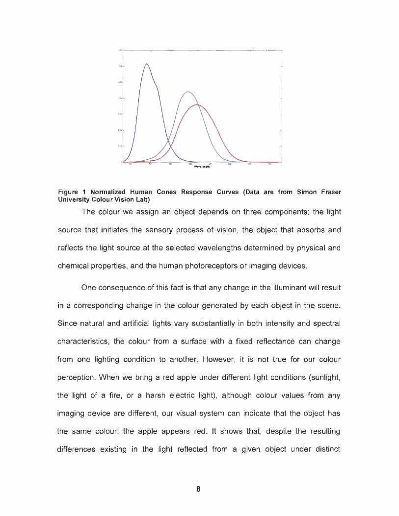
Figure 1 Normalized Human Cones Response Curves (Data are from Simon Fraser University Colour Vision Lab)

The colour we assign an object depends on three components: the light

source that initiates the sensory process of vision, the object that absorbs and

reflects the light source at the selected wavelengths determined by physical and

chemical properties, and the human photoreceptors or imaging devices.

One consequence of this fact is that any change in the illuminant will result

in a corresponding change in the colour generated by each object in the scene.

Since natural and artificial lights vary substantially in both intensity and spectral

characteristics, the colour from a surface with a fixed reflectance can change

from one lighting condition to another. However, it is not true for our colour

perception. When we bring a red apple under different light conditions (sunlight,

the light of a fire, or a harsh electric light), although colour values from any

imaging device are different, our visual system can indicate that the object has

the same colour: the apple appears red. It shows that, despite the resulting

differences existing in the light reflected from a given object under distinct

illumination conditions, the colour that our visual system assigns to the object is

illuminant-independent. This kind of ability that can adjust to widely varying

colours of illumination in order to approximately preserve the appearance of

object colours is called chromatic adaptation [7].

Chromatic adaptation was defined by Wyszecki and Stiles in 1982 [8].

They proposed that the change in the visual response to a colour stimulus is

caused by (a) previous exposure to a conditioning stimulus (such as a luminous

coloured light or intensely coloured surface) or (b) simultaneous presentation of

the colour stimulus against a surround or background of a different colour. During

chromatic adaptation, a significant part appears to take place in the

photoreceptors and cortex, either as a change in the individual sensitivity curves

or in the response of the retinal secondary cells to human cones' outputs.

Figure 2 shows an example of shifts that occur as the illuminant changes

from daylight D65 to incandescent A. The increase in long wavelength light

bleaches proportionally more red information while lowering the green and blue

responses. On the other hand, the decrease in short wavelength light allows

more cones that are sensitive to short wavelength range to regenerate,

increasing the probability of blue responses.

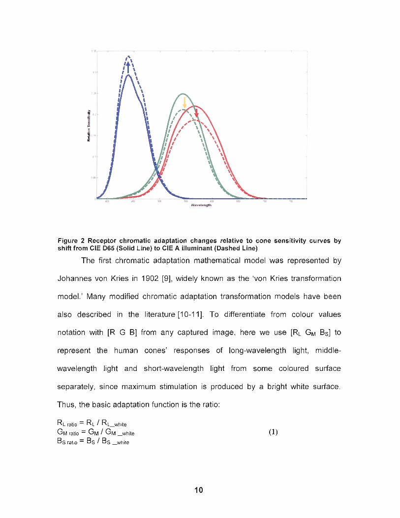
Figure 2 Receptor chromatic adaptation changes relative to cone sensitivity curves by shift from CIE D65 (Solid Line) to CIE A illuminant (Dashed Line)

The first chromatic adaptation mathematical model was represented by

Johannes von Kries in 1902 [9], widely known as the 'von Kries transformation

model.' Many modified chromatic adaptation transformation models have been

also described in the literature [lo-111. To differentiate from colour values

notation with [R G B] from any captured image, here we use [RL GM Bs] to

represent the human cones' responses of long-wavelength light, middle-

wavelength light and short-wavelength light from some coloured surface

separately, since maximum stimulation is produced by a bright white surface.

Thus, the basic adaptation function is the ratio:

Where [RL GM Bs] is human cones' responses under any particular

illumination condition, [RL - white GM - white Bs - white] is responses of same scene under

the white illumination. Because the chromaticity values from the white patch

represent the illumination's colour information, the basic adaptation can also be

applied to predict colour matches across changes in viewing illumination

conditions. For example, if the daylight shifts from illuminant D65 to illuminant A:

Where [RL - A GM - A BS - A] and [RL - D65 GM - 065 BS - 12651 are human's responses

of surface with any colour under illumination A and D65 separately; [RL - ,,(A)

G M - ~ ~ ( A ) BS-wp(A)] and [ R L - W ~ ( D ~ ~ ) Ghn-wp(D65) B~-wp(D65) ] are tNJman's responses of

white patch under illumination A and D65 separately.

Computational colour constancy is an important research field that builds

mathematical models related to human chromatic adaptation. The final objective

of the model is to take full advantage of the full colour information available in the

typical tri-chromatic scene colours and reproduce an accurate colour-constant

estimation of the object. There are many definitions and explanations about

colour constancy. According to the definition from Foster et. al. [12]: "Colour

constancy is the constancy of the perceived colours of surfaces under changes in

the intensity and spectral composition of the illumination." Until now, many

theories of colour constancy explain how the visual system manages to extract

information about the reflectance of the objects in a scene from the colour

signals. Since this involves separating the contribution of the reflectance and the

illuminant in the colour signal, these theories are often characterized as

"discounting the illuminant." Perfect colour constancy in these terms would

involve accurate recovery of reflectance for any scene under any lighting

conditions. The measured colour of objects would be perfectly correlated with

their reflection characteristics and would not vary at all with changes in the

illuminant or the composition and arrangement of objects in view. However, this

type of perfect colour constancy is impossible, since the problem is under

constrained.

CHAPTER 3: SURVEY OF COMPUTATIONAL COLOUR CONSTANCY MODELS

The ultimate stage of the imaging system is to build a mathematical model

embodying the predominant phenomena occurring in the formation of colour

images. Therefore, all of the light source, the object, and the optical system

should be quantified. The light source is represented by its spectral power

distribution E(A), and the coloured materials are quantified through their spectral

distribution of the energy they reflect or transmit SR(A). The optical system is

specified by the spectral sensitivity function Ok(A). A general visual system can

be seen as an array of k sensors. Since the human retina has (or most imaging

devices have) three types of cones (or sensors) that respond to colour radiation

with different spectral response curves, k is always set to be 3, and colour is

specified by a tri-component colour.

Basically, two major processes are involved in colour formation: the colour

signal reaction on the object's surfaces and the camera measurement of the

colour signal coming from the reaction. For the first process, it is necessary to

describe the mutual interaction between light and object, called colour signal.

Colour signal is the product of light spectral power distribution and surface

reflectance at the corresponding individual wavelength, written by C(A) = E(A)*

SR(A). Accounting for the second issue, the way a sensor integrates the colour

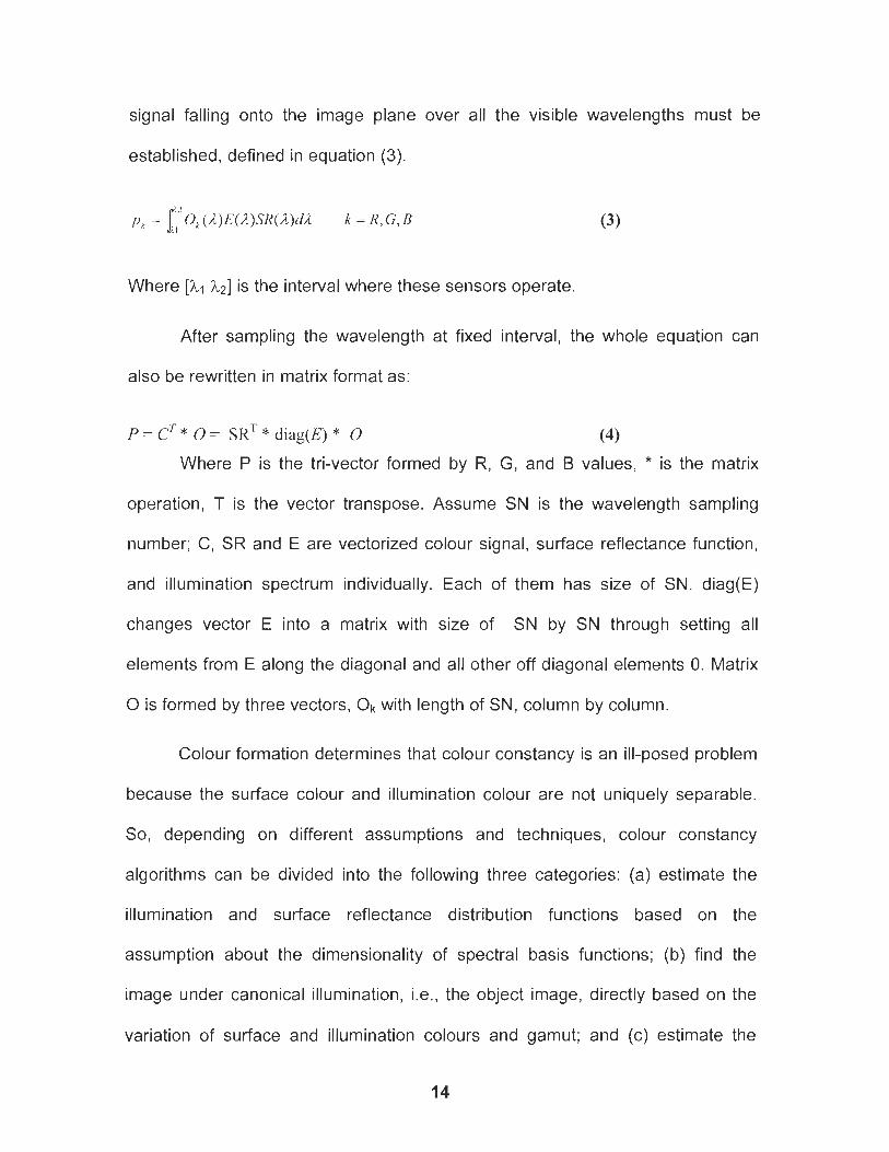
signal falling onto the image plane over all the visible wavelengths must be

established, defined in equation (3).

Where [h, h2] is the interval where these sensors operate.

After sampling the wavelength at fixed interval, the whole equation can

also be rewritten in matrix format as:

p = c T * S R ~ * diag(E) * O (4)

Where P is the tri-vector formed by R, G, and B values, * is the matrix

operation, T is the vector transpose. Assume SN is the wavelength sampling

number; C, SR and E are vectorized colour signal, surface reflectance function,

and illumination spectrum individually. Each of them has size of SN. diag(E)

changes vector E into a matrix with size of SN by SN through setting all

elements from E along the diagonal and all other off diagonal elements 0. Matrix

0 is formed by three vectors, Ok with length of SN, column by column.

Colour formation determines that colour constancy is an ill-posed problem

because the surface colour and illumination colour are not uniquely separable.

So, depending on different assumptions and techniques, colour constancy

algorithms can be divided into the following three categories: (a) estimate the

illumination and surface reflectance distribution functions based on the

assumption about the dimensionality of spectral basis functions; (b) find the

image under canonical illumination, i.e., the object image, directly based on the

variation of surface and illumination colours and gamut; and (c) estimate the

illumination colour based on the assumption about scene colour distribution.

Barnard et.al. compare the performance of various colour constancy solutions

[14,15].

3.1 Finite-Dimensional Linear Model for Colour Constancy

This kind of colour constancy algorithms supposes that illumination and

surface reflectance can be accurately modelled by the dimensionality of the

spectral basis functions [15]. One of the most important works was given by

Maloney and Wandell [ I 6,171.

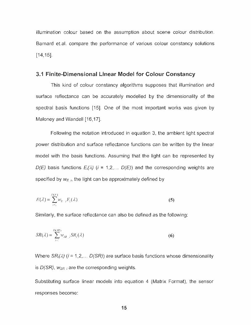
Following the notation introduced in equation 3, the ambient light spectral

power distribution and surface reflectance functions can be written by the linear

model with the basis functions. Assuming that the light can be represented by

D(E) basis functions E,(/Z) ( i = 1,2,. . . D(E)) and the corresponding weights are

specified by WE - ,, the light can be approximately defined by

Similarly, the surface reflectance can also be defined as the following:

Where SRi(/Z) ( i = 1,2,. . . D(SR)) are surface basis functions whose dimensionality

is D(SR), w s ~ - i are the corresponding weights.

Substituting surface linear models into equation 4 (Matrix Format), the sensor

responses become:

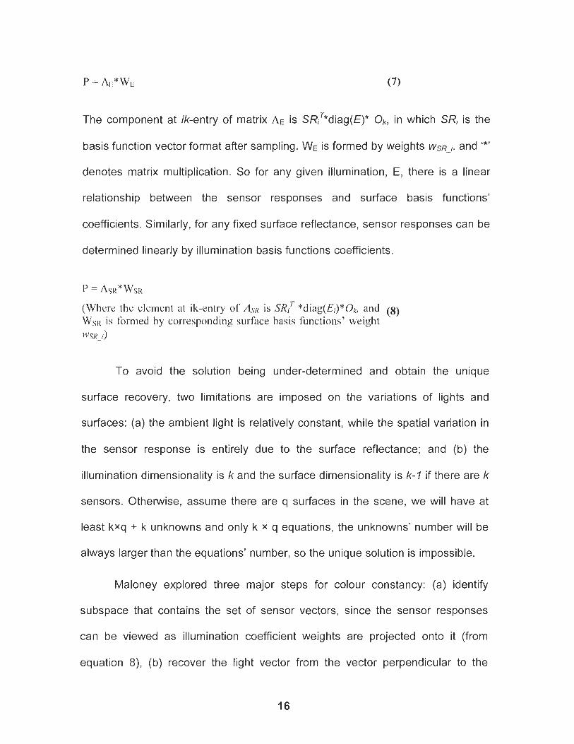
The component at ik-entry of matrix AE is ~ ~ i ~ * d i a ~ ( ~ ) * Ok, in which SRi is the

basis function vector format after sampling. WE is formed by weights WSR - i. and '*'

denotes matrix multiplication. So for any given illumination, E, there is a linear

relationship between the sensor responses and surface basis functions'

coefficients. Similarly, for any fixed surface reflectance, sensor responses can be

determined linearly by illumination basis functions coefficients.

p = A S I ~ * ~ S R

(Where the element at ik-entry of Asn is SR~' *diag(Ei)*Oa, and (8) WSR is formed by corresponding surface basis fiinctions' weight Wylii)

To avoid the solution being under-determined and obtain the unique

surface recovery, two limitations are imposed on the variations of lights and

surfaces: (a) the ambient light is relatively constant, while the spatial variation in

the sensor response is entirely due to the surface reflectance; and (b) the

illumination dimensionality is k and the surface dimensionality is k-I if there are k

sensors. Otherwise, assume there are q surfaces in the scene, we will have at

least kxq + k unknowns and only k x q equations, the unknowns' number will be

always larger than the equations' number, so the unique solution is impossible.

Maloney explored three major steps for colour constancy: (a) identify

subspace that contains the set of sensor vectors, since the sensor responses

can be viewed as illumination coefficient weights are projected onto it (from

equation 8), (b) recover the light vector from the vector perpendicular to the

sensor data, and (c) solve the surface reflectance coefficients through the

function WsR = k * inv(AsR) with the conventional pseudoinvese computation of

matrix As, once the light is known. Further details about the implementation of

the algorithm can be found in [ I 6,171.

Although this solution shows good performance on the Munsell chip

database, it is not practical for the real scenes for two reasons. First, the

illumination and surface should be represented by 2 and 3 basis functions,

respectively, which have been shown to be inaccurate by many researchers.

Cohen [I81 found that Munsell colours depend on 3 or more components. Malony

[ I 91 concluded that 5 to7 basis functions are appropriate. Parkkinen[20] analyzed

1257 reflectance spectra and suggested that 8 basis functions can lead to

accurate reproduction. Laamanen analyzed two illumination and surface

reflectance datasets and demonstrated that at least 10 basis functions are

needed 1211. Second, the variation in surface colour in a three-dimensional colour

space would follow a plane, but these assumptions can only be true under

specifically controlled illumination.

3.2 Object Image Recovery

The object colour image can be viewed as the object under certain

canonical illumination, normally the white illumination with equal energy at all

wavelengths. So given any colour image under unknown illumination,

compensation for the illumination effect on images and recovery of the original

object image is another type of colour constancy solution.

3.2.1 Retinex

Retinex is one of the most famous colour constancy algorithms. It

originated from Land's landmark research work on human vision [22]. Land

proposed that the absolute values of photo-pigment absorption in the eye do not

explain colour appearance. Rather, colour appearance depends on relative

absorption of light by the cones and their spatial pattern in the eye, making vision

independent of the illumination at various locations and dependent instead on the

path followed by the light reaching the eye. He named it 'Retinex' because he

believed that this mechanism comes from the integration of 'retinal' and 'cortex.'

Given a colour image, the basic idea of Retinex is to separate the

illumination from the reflectance image by processing three images lk (k = R,G,B)

independently. If the sensor sensitivity function 0 is sharp enough, i.e. close to

dirac delta function, the intensity value at location (x,y) , Ik(x,y), can be

decomposed into two different values: the illumination image Ek(x,y) and

reflectance image SRk(x,y), thus Ik(x,y) = Ek(x,y) * SRk(x,y). Retinex assumes

spatial smoothness of the illumination field, i.e. the illumination change smoothly

on the scene, while the reflectance image corresponds to the sharp change in

the image.

Retinex computation is always implemented in the log domain so that the

multiplications can be replaced by the additions. If i = log I, e = log E, and sr = log

SR, we have i = e + sr. All of the up-to-date Retinex algorithms have the same

processing framework, except the actual illumination estimation solutions.

The original Retinex algorithm was also proposed by Land. In his solution,

any pixel is selected as the starting pixel. Several paths from the pixel can be

formed by randomly selecting neighbouring pixels. Along each path, the

accumulators of difference between two neighbouring pixels are updated at

pixels, and the total number of accumulators is defined as 'path length'. The final

recovered object image can be obtained through divide the accumulator value at

each pixel by the total paths' number passing it. Therefore, parameters, such as

path length, number of paths, and how a path is calculated, are very important in

'Retinex.' A discussion about their tuning can be found in [22-241.

Since Land proposed this algorithm, many variants of Retinex have been

proposed. Stockham [26] and Faugeeras [27] present that illumination and

surface are low-pass and high-pass results, respectively, after applying a

homomorphic filter on the input image in the logarithmic domain. Horn [28]

formalized Retinex in terms of differentiation, thresholding, and re-integration in

the logarithm domain. Multi-resolution versions of Retinex were introduced for

efficiency [29]. Kimmel[30] adopted a Bayesian view point of the estimation

problem and proposed a variational model for the Retinex problem. This model

can formulate the illumination problem as a Quadratic Programming problem and

can unify previous Retinex solutions. Two versions of Retinex have been given

standardized definitions in terms of Matlab code [23].

3.2.2 Gamut Mapping

Another well-known algorithm is gamut mapping, originally introduced by

Forsyth and extended by Finlayson [31]. The gamut of any illumination is the set

of all possible observed colours under it. If all of these colours are drawn in a

chromaticity space, the gamut is closed, convex, and bounded. Based on the

linear model theory, the goal of gamut mapping to find a transformation matrix

that maps the gamut under unknown illumination to that under canonical

illumination, so that the image colour under canonical illumination can be derived.

Forsyth founded his work on the assumption that scenes consist only of flat,

matte surfaces and that the illumination is spatially constant. The rgb's values

under any illuminant will form a convex hull and change between them are

related by a diagonal matrix. He developed an algorithm, named CRULE, to find

a transformation family. Although CRULE performs very well provided that the

assumed world restrictions are satisfied, it fails when the scenes contain specular

highlights, spatially varying illumination, and surface orientation information. To

address this problem, Finlayson ignored the image intensity information by

mapping the 3D (R,G,B) spaces into 2D chromaticity space. The same CRULE

was run directly on 2D perceptive colours to produce all possible transformations.

Since CRULE can only create a set of feasible maps, the final step is to choose

one to represent the unknown illuminant. One way of doing this is to find the map

that takes all image colours into the canonical gamut such that image colours are

made as colorful as possible, which can be achieved by finding the maximum

area feasible map.

3.3 Illumination Estimation for Colour Constancy Another category of colour constancy is to estimate the illumination

values, either two chromaticity parameters (x,y or r,g) or 3 descriptors (X,Y,Z or

R,G,B). All of these algorithms can be further divided into two groups:

unsupervised estimation and supervised estimation. Unsupervised algorithms

predict the illumination information directly from a single image based on some

assumptions about the general nature of the colour components of images while

supervised ones always include two steps: the first one is to build a statistical

model between the input images and the output known illuminations by learning

training data sets, and the second one is to predict the illumination of any given

image based on the model.

3.3.1 Unsupervised Illumination Estimation

MAXRGB

The MAXRGB algorithm assumes that there is always a white surface in

the scene. The maximal RGB values corresponding to the responses from this

white surface represent the illumination estimations [32]. The MAXRGB solution

can be viewed as a special case of Retinex. Obviously, this method will be

successful providing that a scene contains either a single surface that is

maximally reflective throughout the range of the sensitivity of the imaging device

(i.e., a white surface) or a number of surfaces that are maximally reflective

throughout the range of each of the three imaging sensors individually [33].

In spite of its simplicity, MAXRGB does not give a reasonable

performance for a real world scene because the algorithm's assumption cannot

be easily met.

GRAY WORLD

The Gray-World algorithm assumes that, given an image with a sufficient

number of surface colour variations, or with a uniformly gray surface, the average

value of the surface tends to be gray. The departure from the gray values is

considered the illumination estimations. Therefore, the average RGB in the

image is estimated as the illumination colour [I].

This assumption is generally valid since in any given real world scene, we

often have lots of different colour variations. As the surface colour variations are

random and independent, it would be safe to say that given a large enough

number of samples, the average should converge to the mean value, which is

gray. For instance, if an image were shot with a camera under yellow lighting, the

camera output image would have a yellow cast over the entire image. The effect

of this yellow cast disturbs the Gray-World Assumption of the original image. By

enforcing the assumption on the camera output image, we would be able to

remove the yellow cast and re-acquire the colours of our original scene, fairly

accurately.

Shades of Gray

Max-RGB and Gray-World algorithms will work very well only if the

average scene is gray or a white patch in the scene. G.D. Finlayson et. al. [2]

proposed a more general light colour estimation method with the Minkowski

norm, assuming the image scene appears to be gray after applying an nonlinear

invertible transformation (p-norm function is selected here) at every pixel in each

channel.

Without loss of generality, let's consider the red component of colour

image. All of the red responses can be rewritten into a vector R,. = [R, , R, ,..., R,,,]

with image size of N. The corresponding values are R," = [R,", Rl, ..., R,:] in the n-

power raised image. If the scene of the raised image tends to be gray, the

2R : - 1=I illumination red component value can be estimated by R,, - ,,,iscr, - , and the

A'

illumination value for the original image is R,E =d= . This equation is the

Minkowski norm definition at channel R. We can use a similar method to find the

illumination estimation for channels G and B.

Obviously, Max-RGB and Gray-World algorithms are two instantiations of

the Minkowski norm by setting p = o~ and p = 1, respectively. In this paper [2], the

authors claimed that the algorithm can reach the best performance when the

norm value is set to 6.

Colour Constancy based on Gray-Edge Hypothesis

J. Weijer and Th. Gevers [34] proposed a colour illumination estimation

algorithm assuming that the average of the reflectance difference in a scene is

achromatic.

The authors explained this solution as skewing colour derivatives

distribution such that the average output corresponds to the white light direction

in the opponent colour space. Assuming the colour image value at location (x,y)

is [R(x,y) G(x,y) G(x,y)], the colour derivative value can be represented by :

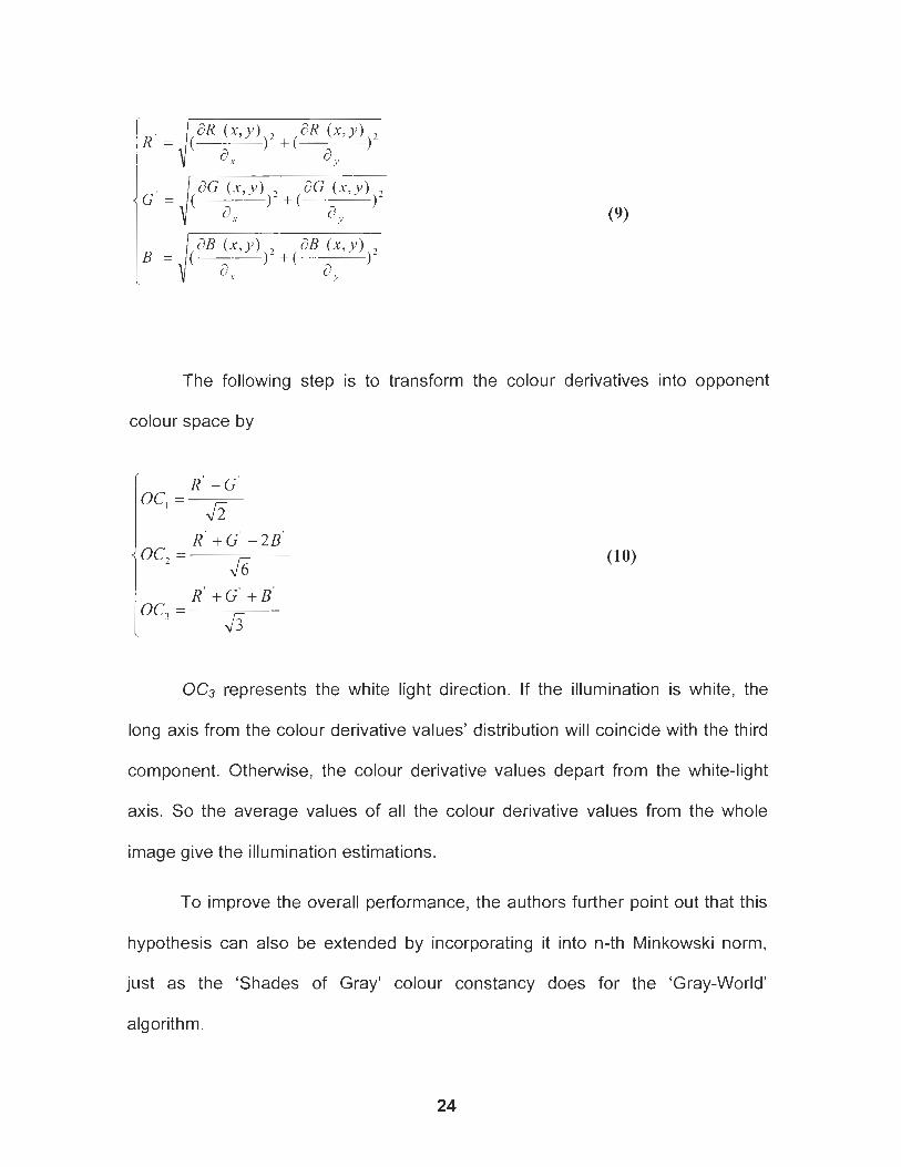
The following step is to transform the colour derivatives into opponent

colour space by

R' - G' OC, = JZ

R' +G' - 2 ~ ' OC, =

&

I R' + G' + B' OC, =

43

OCs represents the white light direction. If the illumination is white, the

long axis from the colour derivative values' distribution will coincide with the third

component. Otherwise, the colour derivative values depart from the white-light

axis. So the average values of all the colour derivative values from the whole

image give the illumination estimations.

To improve the overall performance, the authors further point out that this

hypothesis can also be extended by incorporating it into n-th Minkowski norm,

just as the 'Shades of Gray' colour constancy does for the 'Gray-World'

algorithm.

3.3.2 Supervised Illumination Estimation

Colour by Correlation

Finlayson et.al. has proposed a method, called 'Colour by Correlation,'

that builds the correlation matrix to correlate the probability of image colours with

each possible illuminant [5]. This matrix is built from a large set of colour images

and corresponding known illuminations. To cancel out the effects of intensity,

geometry, and shading, these images' colours are changed into chromaticities

and then mapped to histograms bins. The rows in the matrix are all of predefined

chromaticities, the columns are known illuminants from the training data set, and

the entity in the matrix is the likelihood of an image chromaticity under a given

light. During the test stage, the image colour is transferred into a binary vector in

which '1' or '0' indicates the presence or absence of the corresponding

chromaticity in the image. This vector is a dot-product with each column of the

correlation matrix, and the illumination with the maximal value is predicted to be

the estimation result. The other contribution of this paper [5] is that it proves that

this framework is general and can be used to describe many existing algorithms.

Barnard et. al. [35] improved the promising 'Colour by Correlation' method by

extending it into the 3D colour space. In addition to chromaticity, the extra

information used is pixel brightness.

Neural Network

A multi-layer neural network was established to learn the relationship

between illumination chromaticity and colour distribution in the image, and then

to predict the unknown illumination from an image [3,4]. The training input is the

image chromaticity binary histogram. The (R,G) space is divided into cells 0.02

units wide so that it includes 2500 bins as input layer nodes. ' 7 ' or '0' in each bin

represents the presence or 'absence' of certain chromaticity. The neural net has

two hidden layers: one has 400 nodes and the other has 30 nodes. Two output

nodes with real value are the corresponding illumination chromaticities. It is

trained with the backpropagation algorithm with a sigmoid activation function.

Colour Constancy by KL-Divergence

Many colour constancy algorithms attempt to use a statistical model to

estimate the maximum likelihood values of illumination, C. Tosenberg et, al. use

maximum likelihood and KL-divergence as the solution [36].

Assume [R(x,y)lG(xly)lB(xl~)l and [Rc(x,y),Gc(x,y),Bc(x,~)l are the

responses under an unknown illumination or some canonical illumination for the

same pixel respectively. The Von Kries diagonal transformation can tell us the

relationship between them:

If we ignore only the absolute intensity values of illumination, the colour

constancy problem can be solved by only estimating a and P while restricting y to

be 1.

Considering the image in log-chromaticity space, the illumination change

means colour values shift:

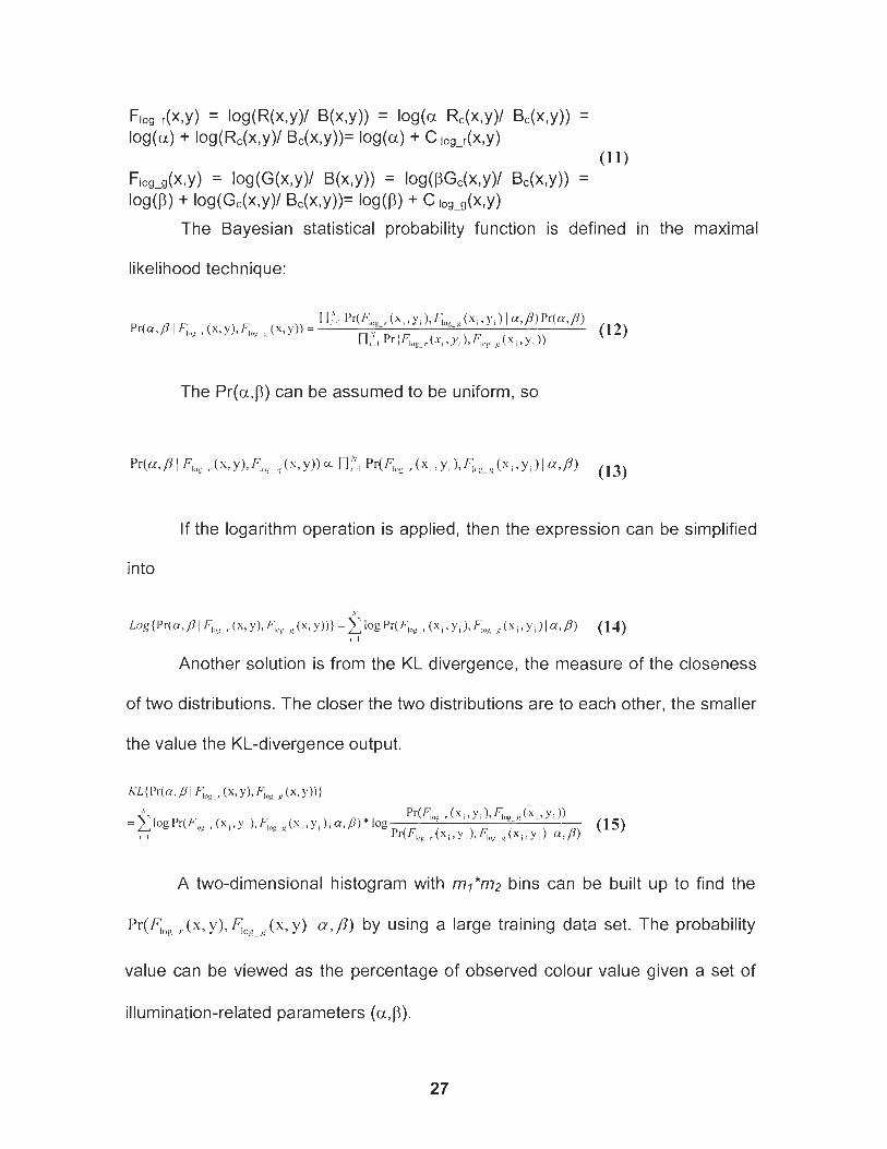
likelihood technique:

The Pr(a,P) can be assumed to be uniform, so

If the logarithm operation is applied, then the expression can be simplified

into

\I

Log{Pr(ff7P1 I;,,,z -- , - (x ,y) ,F I , , , ( x , ~ ) ) } = ~ ~ P I . ( F ~ ~ ~ r ( ~ 1 3 ~ , ) 9 F 1 0 p _ R ( ~ i 7 ~ , ) I u 9 P ) (14) ,-I

Another solution is from the KL divergence, the measure of the closeness

of two distributions. The closer the two distributions are to each other, the smaller

the value the KL-divergence output.

A two-dimensional histogram with ml*m2 bins can be built up to find the

Pr(F,og-,.(~, y), cog - (x, y) I a,P) by using a large training data set. The probability

value can be viewed as the percentage of observed colour value given a set of

illumination-related parameters (a,P).

These two equations look very similar. But the authors point out two major

differences between them: the first one is from the scoring possible matching

functions' definitions between the canonical colour distribution and given colour

image distribution, and the second one is from the conditions when the best

match is reached.

3.4 Multiplicative Cues to Illumination

Each computational colour constancy algorithm can be considered as

applying a potential cue to the illumination present in a scene. However, various

cues are always simultaneously available in the scene that provides valuable

information about colour perception. The human vision system attempts to

combine them, may ignore some in favour of the others, or may attempt to

represent the two as dominant perceptions. These cues not only come from the

colour information in the image but also include the scene background, object

spatial arrangement, surface orientation, binocular disparity, and other factors.

The original research in this field is indebted to the Gilchrist's work in 1977

[37]. He performed a series of experiments to investigate the effect of spatial

arrangement on human lightness constancy and proposed that the retinal ratio

alone cannot tell us the whole story. The simulated scene includes trapezoids

whose perceived orientation and shape are under different viewing conditions. All

of these trapezoids are arranged to be coplanar with one or the other of two

background planes, which were perpendicular to each other. The psychophysical

experiments proved the 'coplanar ratio hypothesis': the perceived lightness of the

object is only controlled by the luminance relationship between coplanar regions

that have same depth; those non-coplanar regions are substantially irrelevant

although they may be retinally adjacent. The luminance relationship between the

target and non-coplanar regions (despite retinal adjacency) is trivial.

Yamauchi and Uchikawa [38] investigated the effects of depth information

on perception by measuring the stimuli's upper-limit luminance in a three-

dimensional environment. In their experiments, the stimulus was presented in

one room, and the observers sat in another room. They were required to adjust

the luminance of a test colour and set the level perceived to be the limit of

surface-colour mode. The test stimulus and those surrounding stimuli composed

of 10 colours were at different spatial locations. The results strongly support the

coplanar importance on the mode of colour perception.

People observe naturally any scene binocularly. So binocular disparity can

also provide a lot of information, especially spatial depth information, which

should be very useful in colour perception. Yang and Shevell [39] found that

binocular disparity improved colour constancy. For their research, they set up a

kind of special equipment that can generate two images displayed on two

monitors controlled by two CPUs. The subject' left and right eyes focused on

separate video displays reflected by two mirrors, positioned so that the viewer

could see a fused image. A keyboard was also prepared to set the matching

chromaticity value of the test patch under different conditions. The experiments

show that the binocular disparity is indeed an important factor in colour

perception.

Another important cue is the orientation of any object's surface. Its

influence on the lightness was examined by Boyaci, Maloney, and Hersh [40]. In

this project, a test patch with seven orientations was used. The scene was lit

under a mixture of diffuse and point light sources. Six observers participated in

the experiment. In each trial, the observer used the mouse to control a

monocular stick-and-circle gradient probe superimposed on the middle of the test

patch, estimate the orientation patch, then match the lightness of the test patch

by choosing one of the reference chips. The experiments showed that human

perception of orientation was nearly veridical.

In addition to depth and binocular disparity, there are other valuable

environmental factors affecting colour perception of any surface. Yang and

Maloney [41] evaluated and determined if the human vision system takes

advantage of three illumination cues: specular light, full surface specularity, and

uniform background. Some specular, coloured spheres were placed on a uniform

plane perpendicular to the experiment participant's sight line. The viewer sat at

the open side, positioned in a chin rest, and gazed at a large, high-resolution

stereoscopic display. Two standard illuminations, D65 and A, lit the scene. The

viewers were required to adjust a small coloured patch until it appeared to be

gray. The achromatic settings from different candidate cue configurations were

evaluated in CIE u'v' space. The experiments showed that colour perception is

affected by several factors to different degrees. The surface specular cue is

significant for illumination, and the other two have trivial influence.

Maloney also proposed a plausible framework for analyzing human

surface colour perception based on the weighted average of illumination cues

1421. The weights corresponding to different cues varied from location to location

within a scene, reflecting the importance of illumination information available from

each type of cue. For example, in the scene with uniform background, little

weight should be given to illumination from background cue. His experiments

show that the cue promotion and dynamic reviewing intervene to assign the

weights.

CHAPTER 4: COLOUR CONSTANCY UNDER UNIFORM ILLUMINATION

lllumination estimation is fundamental to white balancing digital colour

images and to understanding human colour constancy. In this chapter, we will

present three advanced illumination colour estimation solutions: Support Vector

egression', Thin Plate Spline and Gray Surface ldentification2. All of these three

proposed solutions are compared with other published methods, including neural

network colour constancy, colour by correlation, and shades of gray. The

synthetic and real images experiments show that their performances are

comparable to the other colour constancy solutions.

4.1 Introduction

Accurate estimation of the spectral properties of the light illuminating an

imaged scene by automatic means is an important problem. It could help explain

human colour constancy and it would be useful for automatic white balancing in

digital cameras. Here we will focus on machine-based colour constancy. A colour

imaging system will be considered to be colour constant to the degree to which it

is able to account for changes in the colour of the scene illumination and thereby

maintain a stable representation of object colours.

1 The work on this method also appears as a published paper: Weihua Xiong and Brian Funt, "Estimating lllumination Chromaticity via Support Vector Regression", Journal of Imaging Science and Technology, Vol. 50, No. 4, pp. 341-348, JulylAugust 2006

2 These two methods have been submitted for USA and Korean Patents by Samsung Corporation

More precisely we can formulate colour constancy as: Given a digital

image acquired under unknown illumination conditions, predict what the image

would have been if the same scene had been illuminated instead by some

chosen known 'canonical' illuminant. For example, the canonical illuminant might

be specified as equal-energy white. Colour constancy can be divided into two

sub-problems: (a) estimate the colour of the illumination, (b) adjust the image

colours based on the difference between the estimated and canonical

illuminants. The second problem is often addressed by the von Kries coefficient

rule or an equivalent diagonal transformation model [43]. Because it is very under

constrained, the first problem, illumination estimation, is the more difficult of the

two. Here we will introduce three new solutions: Support Vector R.egression,

Thin Plate Splim, and Gray Surface Identification. The first two cstiinate the

illuini~lation clironlaticity values while tlic third one gives out, the illumination

coloriirletric values.

4.2 lllumination Chromaticity Estimation by Support Vector Regression

lllumination chromaticity estimation from support vector regression is

similar to previous work by Funt et. al. 14,441 and Finlayson et. al. [5] in that it

aims to recover the chromaticity of the scene illumination based on the statistical

properties of binarized colour or chromaticity histograms; however, the proposed

method replaces the neural networks and Bayesian statistics of these previous

methods with support vector machine regression.

Vapnik's [45,46] Support Vector Machine theory has been applied

successfully to a wide variety of classification problems [47-501. Support vector

machines have been extended as well to regression problems including financial

market forecasts, travel time prediction, power consumption estimation, and

highway traffic flow prediction [51-531.

Depending on the problem domain, support vector machine based

regression (SVR) can be superior to traditional statistical methods in many ways.

SVR enables inclusion of a minimization criterion into the regression, training can

be easier, and it achieves a global rather than local optimum. It also facilitates

explicit control of the tradeoffs between regression complexity and error.

4.2.1 Support Vector Regression Introduction

SVR estimates a continuous-valued function that encodes the

fundamental interrelation between a given input and its corresponding output in

the training data. This function then can be used to predict outputs for given

inputs that were not included in the training set. This is similar to a neural

network. However, a neural network's solution is based on empirical risk

minimization. In contrast, SVR introduces structural risk minimization into the

regression and thereby achieves a global optimization, while a neural network

achieves only a local minimum [54].

Most classical regression algorithms require knowledge of the expected

probability distribution of the data. Unfortunately, in many cases, this distribution

is not known accurately. Furthermore, many problems involve uncertainties such

that it is insufficient to base a decision on the event probability alone.

Consequently, it is important to take into account the potential cost of errors in

the approximation. SVR minimizes the risk without prior knowledge of the

probabilities.

Smola and Scholkopf [45] provide an introduction to SVR. Some simple

intuition about it can be gained by comparison to least-squares regression in

fitting a line in 2-dimensions. Least squares regression minimizes the sum of

squares distance between the data points and the line. SVR maximizes the

space containing the data points subject to the minimization of the distance of the

points to the resulting line. The width of the space is called the 'margin'. Points

within an 'insensitivity' region are ignored. The technique represents the region

defined by the margin by a subset of the initial data points. These data points are

called the support vectors. A linear SVR example for a set of data points is

shown in figure 3.

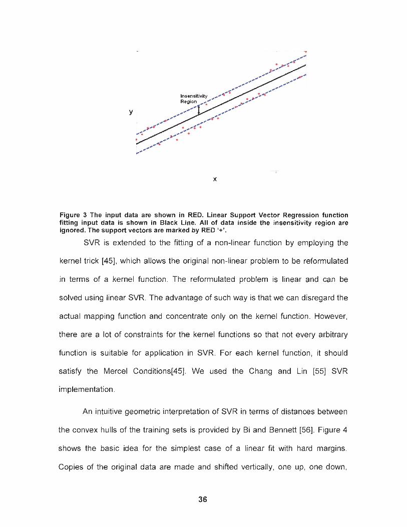
Figure 3 The input data are shown in RED. Linear Support Vector Regression function fitting input data is shown in Black Line. All of data inside the insensitivity region are ignored. The support vectors are marked by RED '+'.

SVR is extended to the fitting of a non-linear function by employing the

kernel trick [45], which allows the original non-linear problem to be reformulated

in terms of a kernel function. The reformulated problem is linear and can be

solved using linear SVR. The advantage of such way is that we can disregard the

actual mapping function and concentrate only on the kernel function. However,

there are a lot of constraints for the kernel functions so that not every arbitrary

function is suitable for application in SVR. For each kernel function, it should

satisfy the Mercel Conditions[45]. We used the Chang and Lin [55] SVR

implementation.

An intuitive geometric interpretation of SVR in terms of distances between

the convex hulls of the training sets is provided by Bi and Bennett [56]. Figure 4

shows the basic idea for the simplest case of a linear fit with hard margins.

Copies of the original data are made and shifted vertically, one up, one down,

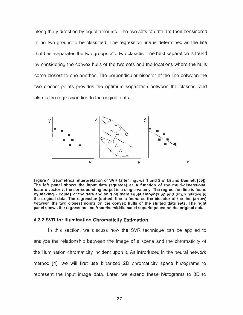
along the y direction by equal amounts. The two sets of data are then considered

to be two groups to be classified. The regression line is determined as the line

that best separates the two groups into two classes. The best separation is found

by considering the convex hulls of the two sets and the locations where the hulls

come closest to one another. The perpendicular bisector of the line between the

two closest points provides the optimum separation between the classes, and

also is the regression line to the original data.

Figure 4 Geometrical interpretation of SVR (after Figures 1 and 2 of Bi and Bennett [56]). The left panel shows the input data (squares) as a function of the multi-dimensional feature vector v, the corresponding output is a single value y. The regression line is found by making 2 copies of the data and shifting them equal amounts up and down relative to the original data. The regression (dotted) line is found as the bisector of the line (arrow) between the two closest points on the convex hulls of the shifted data sets. The right panel shows the regression line from the middle panel superimposed on the original data.

4.2.2 SVR for Illumination Chromaticity Estimation

In this section, we discuss how the SVR technique can be applied to

analyze the relationship between the image of a scene and the chromaticity of

the illumination chromaticity incident upon it. As introduced in the neural network

method [4], we will first use binarized 2D chromaticity space histograms to

represent the input image data. Later, we extend these histograms to 3D to

include intensity as well as chromaticity. Chromaticity histograms have the

potential advantage that they discard intensity shading, which varies with the

surface geometry and viewing direction, but is most likely unrelated to the

illumination's spectral properties.

The training set consists of histograms of many images along with the

measured rg chromaticities (r=R/(R+G+B) and g=G/(R+G+B)) of the

corresponding scene illuminants. Each image's binarized chromaticity histogram

forms an SVR binary input vector in which each component corresponds to a

histogram bin. A '1' or '0' indicates that the presence or absence of the

corresponding chromaticity in the input image. Partitioning the chromaticity space

equally along each component into N equal parts yields N x N bins. The resulting

SVR binary input vector is of size N ~ . We experimented with various alternative

choices for N and eventually settled on N=50. Generally speaking, for N<50, the

bins are too large so the colour space is quantized too coarsely, with the result

that the illumination estimation error increases. For N>50, the training time

increases, but without a corresponding improvement in overall performance. All

the results reported below are based on N=50, so the chromaticity step size is

0.02. With o 2 1;s s rand r+g = I -b < I, only half these bins can ever be filled, so a

sparse matrix representation was used. Support vector regression then finds the

function mapping from image histograms to illuminant chromaticities.

Since some other illumination estimation methods [14,15,57] (gamut

mapping and colour by correlation) benefit from the inclusion of intensity data, it

is natural to consider it in the SVR case as well. The neural network method has

thus far not been applied to 3D data (chromaticity plus intensity) because the

number of input nodes becomes too large and the space too sparse for

successful training, given the relatively small size of the available training sets.

Support vector regression handles sparse data reasonably well, so we

experimented with 3D binarized histograms in the training set. Intensity, defined

as L = R + G + B, becomes the third histogram dimension along with the r and g

chromaticity. We quantized L into 25 equal steps, so the 3D histograms consist

of 62,500 (25x50~50) bins.

4.2.3 Histogram Construction

To increase the reliability of the histograms, the images are pre-processed

to reduce the effects of noise and pixels straddling colour boundaries. We have

chosen to follow the region-growing segmentation approach described by

Barnard et, al. [14,15], in which each pixel that does not belong to any created

region will be used as seed. Each segmented region will correspond to one

histogram bin, and those regions with very few pixels will be ignored, since they

will be considered noisy. This also facilitates comparison of the SVR method to

the other colour constancy methods Barnard et. al. tested. The region-growing

method is good because the borders it finds are perfectly thin and connected.

Membership in a region is based on chromaticity and intensity. A region is only

considered to be meaningful if it has a significant area. For the sake of easy

comparison, we used the same thresholds as 1141; namely, to be in the same

region, the r and g chromaticities at a pixel must not differ from their respective

averages for the region containing the pixel by more than 0.5%, or its intensity by

10%. Also, regions that result in an area of fewer than 5 pixels are discarded.

The RGB's of all pixels within each separate region are then averaged, converted

to L, r, g and histogrammed.

4.2.4 K-Fold Cross Validation for SVR Parameters

The performance of SVR is known to depend on its insensitivity parameter

E, regularization parameter C, the choice of kernel function and associated

parameters. Different kernel functions work better on some problem domains

than others. Four of the commonly used kernel functions are listed in Table 1.

From a practical and empirical standpoint, the bigger the insensitivity parameter

E , the fewer the support vectors, and the higher the error in estimating the

illumination. After much experimentation with different E values, we fixed it to be

0.0001.

Table 1 Admissible Kernel Functions

Name Linear Polynomial

Radial Basis Function (RBF)

Sigmoid*

In the case of SVR for illumination estimation, the best choice of kernel

function and its parameters may depend on the training set. We eliminated the

Sigmoid kernel function from further consideration since it is known to be invalid

for some values of the parameter rr [46] and focus instead on the RBF and

polynomial kernel functions. This leaves the choice of either the RBF or

(*: For some rr values, the kernel function is invalid)

Definition K(x,,xJ = (x;) 'xi K(x,,xJ = [(x3 'x i+ lP

K(x,, xj) = e-711~'~-xl 11' K(x,, xJ =tanh[(xJ ' xi+rr]

Parameters. ---

d

j/

rr

polynomial kernel functions and for each of these kernels their parameters:

penalty C and width y for the RBF kernel function; or penalty C and exponential

degree d for polynomial kernel function. The parameters y and d control the

corresponding kernel function's shape, while C determines the penalty cost of

estimation errors. The kernel choice and parameter settings are made during the

training phase by k-fold cross validation, which involves running the training

using several different parameter choices and then selecting the choice that

works best for that particular training set. This is described in more detail below.

For the RBF kernel function, we allow the penalty parameter to be chosen

from 4 different values C ~ ( 0 . 0 1 , 0.1, 1, 10) and the width value from y ~(0 .025 ,

0.05, 0.1, 0.2). For the polynomial kernel function, we used the same 4 penalty

candidates and selected the best degree d from the set (2 3 4 5). Thus for each

training data set, 32 test cases (2 kernel choices with 16 pairs of parameter

settings each) are tested to find the best choice.

Among the algorithms generally used to find the best parameters for

support vector regression, we chose k-fold cross validation because it does not

depend on a priori knowledge or user expertise and it handles the possibility of

outliers in the training data. The disadvantage of the k-fold method is that it is

computationally intensive.

In k-fold cross validation, the whole training set is divided evenly into k

distinct subsets. Every kernel function and each of its related parameters forms a

candidate parameter setting. For any candidate parameter setting, we conduct

the same process k times during which (k-I) of the subsets are used to form a

training set and the remaining subset is taken as the test set. The RMS

chromaticity distance errors from k trials are averaged to represent the error for

that candidate parameter setting. The parameter setting leading to the minimum

error is then chosen and the final SVR training is done using the entire training

set based on the chosen parameter setting.

4.3 Illumination Colour Estimation Using Thin Plate Splines

A new approach basing on the technique of thin-plate interpolation to

illumination estimation for colour constancy and automatic white balancing is

developed in this section. In this method, we will treat illumination estimation as a

problem of interpolation over a set of training images

Interpolation is a common problem and there are many well-established

interpolation methods[58]. The majority of these methods, such as bilinear or bi-

cubic interpolation, are based on interpolation over training data sampled on a

uniform grid. However, we map image information to illumination r-chromaticity

and g-chromaticity values and use the image's r and g chromaticity values as

inputs. We can not uniformly sample the space of images because the difference

between any two images' chromaticity values is not fixed, so interpolation over a

non-uniformly sampled space is required. Thin-plate spline interpolation is an

effective interpolation method under these conditions, and has been widely used

in the context of deforming one image into registration with another.

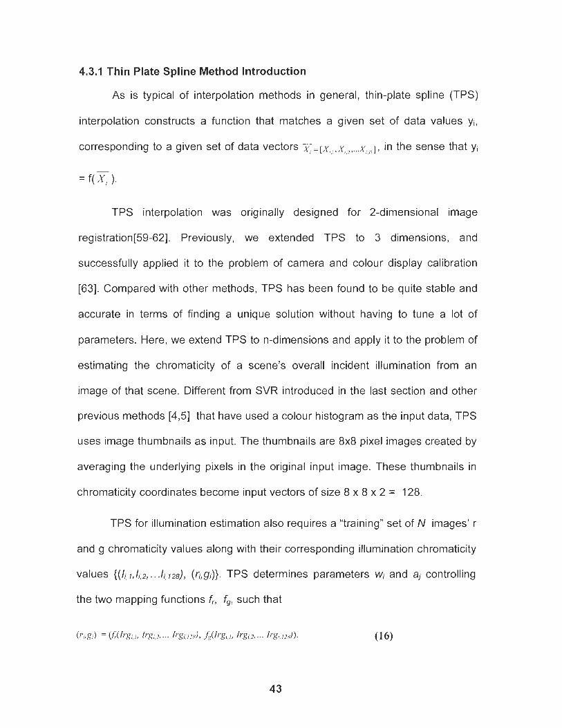
4.3.1 Thin Plate Spline Method Introduction

As is typical of interpolation methods in general, thin-plate spline (TPS)

interpolation constructs a function that matches a given set of data values yi,

corresponding to a given set of data vectors T=[X. ,.I ,?,... x i,,, 1 , in the sense that yi

= f(x,).

TPS interpolation was originally designed for 2-dimensional image

registration[59-621. Previously, we extended TPS to 3 dimensions, and

successfully applied it to the problem of camera and colour display calibration

[63]. Compared with other methods, TPS has been found to be quite stable and

accurate in terms of finding a unique solution without having to tune a lot of

parameters. Here, we extend TPS to n-dimensions and apply it to the problem of

estimating the chromaticity of a scene's overall incident illumination from an

image of that scene. Different from SVR introduced in the last section and other

previous methods [4,5] that have used a colour histogram as the input data, TPS

uses image thumbnails as input. The thumbnails are 8x8 pixel images created by

averaging the underlying pixels in the original input image. These thumbnails in

chromaticity coordinates become input vectors of size 8 x 8 x 2 = 128.

TPS for illumination estimation also requires a "training" set of N images' r

and g chromaticity values along with their corresponding illumination chromaticity

values {(li,l,li,2,. . .livl28)1 (fi,g;)}. TPS determines parameters wi and a, controlling

the two mapping functions f , f,, such that

The mapping function f,, is defined as

where Ci(,r) = x' logr

The function f, is defined similarly. The weights wi control a non-linear

term, and the a,, control an additional linear term.

Each training set pair (an image plus its illumination chromaticity) provides

2 equations. For the th training image we have

In addition, a smoothness constraint is imposed by minimizing the bending

energy. In the original TPS formulation [59], the bending energy function was

defined in 2D. Here we generalize it to higher dimensions defined as a, (i=

1.. 128)

whereJ(j;.) is the total bending energy described in terms of the curvature of f . .

Following [60-621, the energy will be minimized when

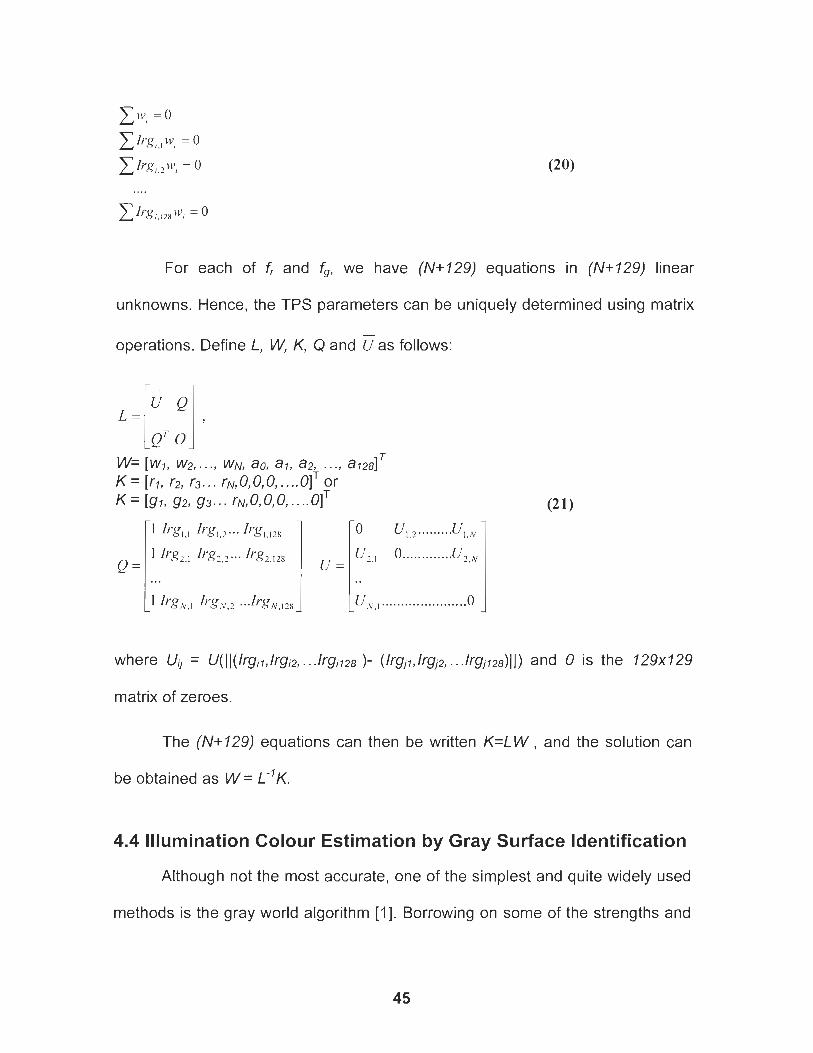
For each of f, and f,, we have (N+129) equations in (N+129) linear

unknowns. Hence, the TPS parameters can be uniquely determined using matrix

operations. Define L, W, K, Q and Gas follows:

The (N+129) equations can then be written K=LW, and the solution can

be obtained as W = L-'K.

4.4 Illumination Colour Estimation by Gray Surface Identification

Although not the most accurate, one of the simplest and quite widely used

methods is the gray world algorithm [I]. Borrowing on some of the strengths and

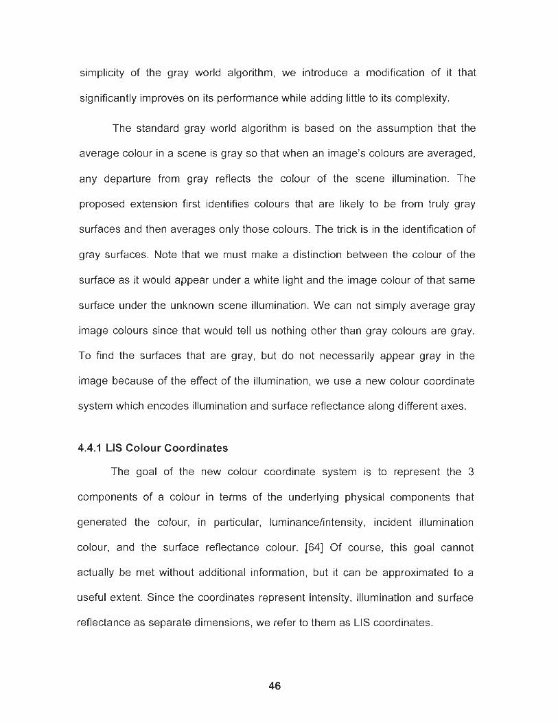
simplicity of the gray world algorithm, we introduce a modification of it that

significantly improves on its performance while adding little to its complexity.

The standard gray world algorithm is based on the assumption that the

average colour in a scene is gray so that when an image's colours are averaged,

any departure from gray reflects the colour of the scene illumination. The

proposed extension first identifies colours that are likely to be from truly gray

surfaces and then averages only those colours. The trick is in the identification of

gray surfaces. Note that we must make a distinction between the colour of the

surface as it would appear under a white light and the image colour of that same

surface under the unknown scene illumination. We can not simply average gray

image colours since that would tell us nothing other than gray colours are gray.

To find the surfaces that are gray, but do not necessarily appear gray in the

image because of the effect of the illumination, we use a new colour coordinate

system which encodes illumination and surface reflectance along different axes.

4.4.1 LIS Colour Coordinates

The goal of the new colour coordinate system is to represent the 3

components of a colour in terms of the underlying physical components that

generated the colour, in particular, luminance/intensity, incident illumination

colour, and the surface reflectance colour. [64] Of course, this goal cannot

actually be met without additional information, but it can be approximated to a

useful extent. Since the coordinates represent intensity, illumination and surface

reflectance as separate dimensions, we refer to them as LIS coordinates.

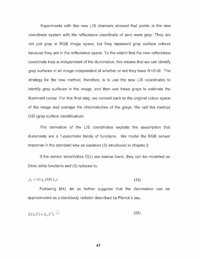
Experiments with this new LIS channels showed that points in the new

coordinate system with the reflectance coordinate of zero were gray. They are

not just gray in RGB image space, but they represent gray surface colours

because they are in the reflectance space. To the extent that the new reflectance

coordinate truly is independent of the illumination, this means that we can identify

gray surfaces in an image independent of whether or not they have R=G=B. The

strategy for the new method, therefore, is to use the new LIS coordinates to

identify gray surfaces in the image, and then use these grays to estimate the

illuminant colour. For this final step, we convert back to the original colour space

of the image and average the chromaticities of the grays. We call this method

GSI (gray surface identification)

The derivation of the LIS coordinates exploits the assumption that

illuminants are a I-parameter family of functions. We model the RGB sensor

response in the standard way as equation (3) introduced in chapter 2

If the sensor sensitivities O(h) are narrow band, they can be modelled as

Dirac delta functions and (3) reduces to,

p, = E(/Z, )SR(/Z, ) (22)

Following [64], let us further suppose that the illumination can be

approximated as a blackbody radiator described by Planck's law,

I is the power of illumination, T is the blackbody radiator temperature, and

the constants cl and cp are 3.741 83*1 o ' ' ~ w ~ ~ and 1.4388*1 o - ~ ~ K , respectively.

Equation (23) becomes

Taking logarithms, we have

C' log(pk ) = log I + log(SR(A, )) -I-+ log(cl/2,')

7-4 (25)

Equation (24) imposes a constraint such that the log of camera responses

[log(R), log(G), log(B)] for a given surface reflectance are confined to a plane. To

see this, let n, = c', 11, and tn, = IO~(C,A;~)+ log(SR(il,)) and substitute into the

equations for log(k). After combining the equations and eliminating the terms log

I and IIT, we obtain

I 1 (I+---- ' I B ) I O ~ R - - 1711 - n t l log G - log B = 1 1 1 , + I I , , I ? I ~ , - I I , ~ I N , + nUmM

n(, - 1 1 ~ n ( , - ) I! , I I ~ , - l l t l I I ( , - r 7 , (26)

Since the nk are fixed by the choice of camera sensitivity, and mk are fixed

by the choice of camera and surface reflectance, for any given surface

reflectance, varying the illumination's colour temperature, T, or its intensity, I,

causes [log(R), log(G), log(B)] to move within a plane. For a different surface

reflectance, a parallel plane is generated. The axis perpendicular to these

parallel planes becomes the reflectance axis of the LIS coordinates.

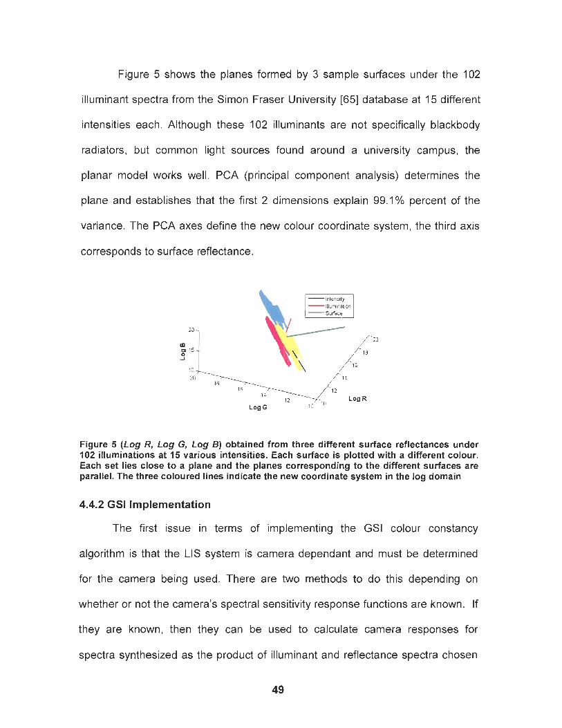
Figure 5 shows the planes formed by 3 sample surfaces under the 102

illuminant spectra from the Simon Fraser University [65] database at 15 different

intensities each. Although these 102 illuminants are not specifically blackbody

radiators, but common light sources found around a university campus, the

planar model works well. PCA (principal component analysis) determines the

plane and establishes that the first 2 dimensions explain 99.1% percent of the

variance. The PCA axes define the new colour coordinate system, the third axis

corresponds to surface reflectance.

Figure 5 (Log R, Log G, Log B) obtained from three different surface reflectances under 102 illuminations at 15 various intensities. Each surface is plotted with a different colour. Each set lies close to a plane and the planes corresponding to the different surfaces are parallel. The three coloured lines indicate the new coordinate system in the log domain

4.4.2 GSI Implementation

The first issue in terms of implementing the GSI colour constancy

algorithm is that the LIS system is camera dependant and must be determined

for the camera being used. There are two methods to do this depending on

whether or not the camera's spectral sensitivity response functions are known. If

they are known, then they can be used to calculate camera responses for

spectra synthesized as the product of illuminant and reflectance spectra chosen

from a database of spectra. If the camera's spectral sensitivity curves are not

known, then real values can be obtained by using the camera to take images of a

gray card under several different illuminants. PCA is then applied to the

logarithms of RGBs from the gray card. The vector corresponding to the maximal

eigenvalue forms the intensity axis, the next vector forms the illumination axes,

and the vector corresponding to the least eigenvalue is the surface reflectance

axis. We have conducted an experiment with Barnard's [65] 321 images

captured using a calibrated SONY DXC-930 camera. These images are from 33

different scenes under 11 different lights that represent a cross-section of

common lights. Since the spectral sensitivity functions of the camera are known

and the calibration images are available on the Internet [65], this data set

provides a means of comparing LIS coordinates extracted based on synthetic

versus on real data. For the synthetic case, we synthesize RGB values for the

measured percent spectral reflectance of 24 Macbeth Colour Checker patches

and the spectral power distributions of 102 illuminants at 15 different intensities

values. Applying PCA to this data, we find the LIS axes as row vectors:

[0.5994 0.5871 0.54411, [0.6421 0.0482 -0.76511, [0.4729 -0.81 32 0.33581.

To compute the LIS coordinates from real data, we have the RGB values

from the gray card under the 11 different illuminants The LIS axes are:

Clearly, the two methods produce very similar results. The advantage of

the real data method is that it is much easier to collect images of a gray card

under a dozen or so different illuminants than it is to determine a camera's

spectral sensitivity functions.

To estimate the illumination for an image of N pixels [Ri,GilBi], each pixel

is first classified as to whether or not it belongs to the class of gray pixels. To

classify a pixel, the logarithm of each channel is taken producing

[logR,,logG,,logBj] which is then projected onto the S axis of the LIS coordinate

system via vector inner product. If the resulting value is less than a specified

threshold value then the pixel is classified as gray.

The GSI method estimates the colour [Re,Ge,B,] of an image's illumination

according to

$ isgru.y([Ri, Gi , B, I) then w, = 1 else W; = 0

where 'isgray' is the test that classifies pixels as gray or not.

An example of the GSI method is shown in Figure 6. The isgray test

identifies as gray those pixels from Figure 6(a) that are shown in white in Figure

6(b)). The true scene illumination as measured from a gray card is [0.2476,

0.2910, 0.46141. The standard gray world method averages the RGBs of all

pixels so that the estimated illumination is found to be [0.4748, 0.2348, 0.29031.

Figure 6(c) shows the result of colour balancing the colours using this gray world

estimate. The GSI method, however, averages only the RGB of pixels that pass

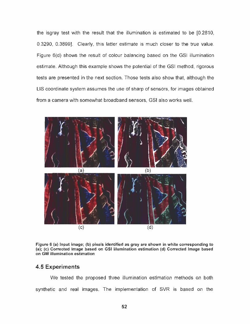
the isgray test with the result that the illumination is estimated to be l0.2810,

0.3290, 0.38991. Clearly, this latter estimate is much closer to the true value.

Figure 6(d) shows the result of colour balancing based on the GSI illumination

estimate. Although this example shows the potential of the GSI method, rigorous

tests are presented in the next section. Those tests also show that, although the

LIS coordinate system assumes the use of sharp of sensors, for images obtained

from a camera with somewhat broadband sensors. GSI also works well.

Figure 6 (a) Input image; (b) pixels identified as gray are shown in white corresponding to (a); (c) Corrected lmage based on GSI illumination estimation (d) Corrected lmage based on GW illumination estimation

4.5 Experiments

We tested the proposed three illumination estimation methods on both

synthetic and real images. The implementation of SVR is based on the

implementation by Chang and Lin [55]. To this we added a Matlab interface that

reads data files representing the image histograms and associated illumination

chromaticities. Each row in the training data file represents one training image

and consists of two parts: the true illumination chromaticity followed by the bin

number for each non-zero histogram bin. TPS and GSI method were

implemented in MATLAB 7.0.1 [66]

Barnard et. al. [ l 4 , l5 ] reported tests of several illumination estimation

methods, including neural-network and colour by correlation based on binary

histogram. For SVR, We have tried to follow their experimental procedure as

closely as possible and used the same image data so that it can be compared

fairly to these other methods. For TPS, the original image will be averaged into

8*8 thumbnail images and changed into chromaticity space as input. In addition,

we compare all of these methods to the "shades of gray" (SoG) technique [2]

based on the Minkowski family of norms, Max RGB and Grayworld.

4.5.1 Error Measures

Several different error measures are used to evaluate performance. The

first is the distance between the actual (ra,ga) and estimated chromaticity of the

illuminant (re,ge) as [14,15]:

For the distance error, we also compute the root mean square (RMS),

mean, and median errors over a set of N test images. It has been argued that the

median is the most appropriate metric for evaluating colour constancy[67]. The

standard RMS is defined as:

The second error measure is the angular error between the chromaticity 3-

vectors when the b-chromaticity component is included. Given rand g, b = 1 - r -

g. Thus, we can view the real illumination and estimated illumination as two

<r,g,b> vectors in 3D chromaticity space and calculate the angle between them.

The angular error represented in degrees is:

We also compute the RMS, mean, and median angular error over a set of

images.

Even if the median angular error for one method is less than for another,

the difference may not be statistically significant. To evaluate whether a

difference is significant, we use the Wilcoxon signed-rank test based on the

angular errors[67]. In the following experiments, the error rate for accepting or

rejecting null hypothesis is always set to 0.01.

4.5.2 Synthetic Data Training, Real-Data Testing

The first tests are based on training with synthesized image data

constructed using the 102 illuminant spectra and 1995 reflectances described by

Barnard [I51 along with the sensor sensitivity functions of the calibrated SONY

DXC-930 CCD[68]. Testing is based on Barnard1s[14] 321 real images taken with

the SONY DXC-930 of 30 scenes under 11 different light sources. These images

are linear (a gamma of 1.0) with respect to scene intensity. This data is available

on-line from the Simon Fraser University Computational Vision Laboratory colour

image database[69].

The number of distinct synthesized training 'scenes' was varied from 8 to

1024 in order to study the effect of training size on performance. Each synthetic

scene was 'lit' by each of the 102 illuminants in turn to create 102 images of each

scene.

For SVR, all of these synthesized camera RGB values, their

corresponding chromaticities, and the illuminant chromaticity are mapped to 2D

and 3D binary vectors for input to SVR. Table 2 shows that the parameters vary

with the training set as expected. Although the basis function type was allowed to

vary during the cross-validation, the RBF was eventually selected in all cases.

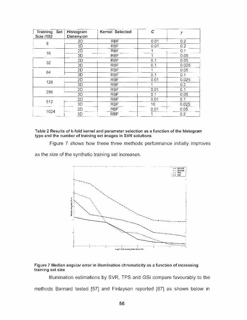
Training Set Size I1 02

8

16

32

Table 2 Results of k-fold kernel and parameter selection as a function of the histogram type and the number of training set images in SVR solutions

Histogram Dimension

2D 3D 2D 3D 2D 3D

64

128

256

51 2

1024

Figure 7 shows how these three methods performance initially improves

2D 3D 2 D 3D

RBF RBF RBF RBF

as the size of the synthetic training set increases.

Kernel Selected

RBF RBF RBF RBF RBF RBF

2 D 3D 2D 3 D 2D 3D

Figure 7 Median angular error in illumination chromaticity as a function of increasing training set size

1 0.1 0.01 1

Illumination estimations by SVR, TPS and GSI compare favourably to the

C

0.01 0.01 1 1 0.1 0.1

0.05 0.1 0.025 0.2

RBF RBF RBF RBF RBF RBF

methods Barnard tested [57] and Finlayson reported [67] as shown below in

Y

0.2 0.2 0.1 0.05 0.05 0.025

0.01 0.1 0.01 10 0.01 1

0.1 0.05 0.1 0.025 0.05 0.2

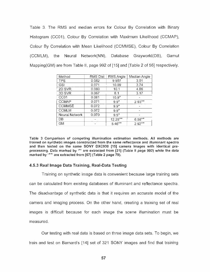
Table 3. The RMS and median errors for Colour By Correlation with Binary

Histogram (CCOI), Colour By Correlation with Maximum Likelihood (CCMAP),

Colour By Correlation with Mean Likelihood (CCMMSE), Colour By Correlation

(CCMLM), the Neural Network(NN), Database Grayworld(DB), Gamut

Mapping(GM) are from Table ll, page 992 of [ I 51 and [Table 2 of 561 respectively.

Method I RMS Dist I RMS Angle 1 Median Angle

GS I

I CCMMSE 1 0.072 1 9.9' 1 I

3.01 TPS

3D SVR CCOl CCMAP

0.071

Table 3 Comparison of competing illumination estimation methods. All methods are trained on synthetic images constructed from the same reflectance and illuminant spectra and then tested on the same SONY DXC930 [I51 camera images with identical pre- processing. Data marked by ' * ' are extracted from 1311 (Table II page 992) while the data marked by I * * ' are extracted from [67] (Table 2 page 79).

0.082

0.067 0.081 0.071

CCMLM Neural Network

4.5.3 Real Image Data Training, Real-Data Testing

9.907 10.09

2D SVR.

Training on synthetic image data is convenient because large training sets

3.74 0.080 10.1

8.1 10.9' 9.9' - -

can be calculated from existing databases of illuminant and reflectance spectra.

4.86 3.17

2.93"

0.072

The disadvantage of synthetic data is that it requires an accurate model of the

9.9'

camera and imaging process. On the other hand, creating a training set of real

images is difficult because for each image the scene illumination must be

0.070

measured.

9 5'

Our testing with real data is based on three image data sets. To begin, we

train and test on Barnard's [I41 set of 321 SONY images and find that training

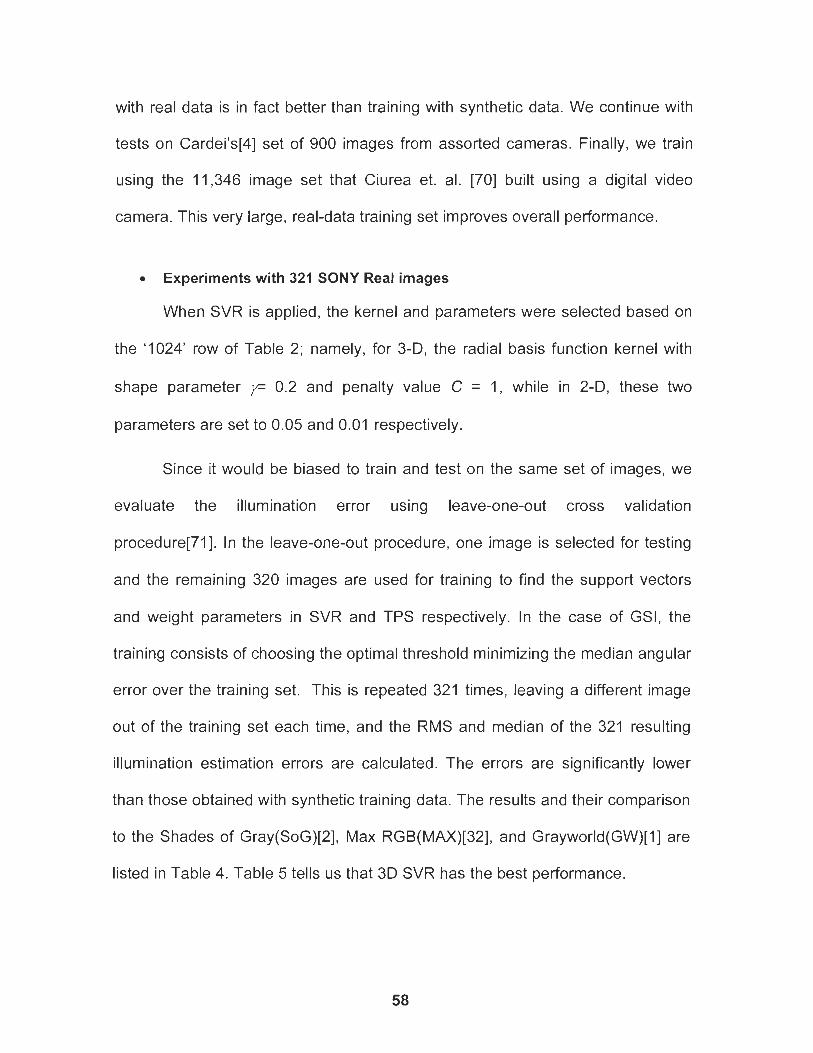
with real data is in fact better than training with synthetic data. We continue with

tests on Cardei1s[4] set of 900 images from assorted cameras. Finally, we train

using the 11,346 image set that Ciurea et. al. [70] built using a digital video

camera. This very large, real-data training set improves overall performance.

Experiments with 321 SONY Real images

When SVR is applied, the kernel and parameters were selected based on

the '1024' row of Table 2; namely, for 3-D, the radial basis function kernel with

shape parameter i / r 0.2 and penalty value C = 1, while in 2-0, these two

parameters are set to 0.05 and 0.01 respectively.

Since it would be biased to train and test on the same set of images, we

evaluate the illumination error using leave-one-out cross validation

procedure[71]. In the leave-one-out procedure, one image is selected for testing

and the remaining 320 images are used for training to find the support vectors

and weight parameters in SVR and TPS respectively. In the case of GSI, the

training consists of choosing the optimal threshold minimizing the median angular

error over the training set. This is repeated 321 times, leaving a different image

out of the training set each time, and the RMS and median of the 321 resulting

illumination estimation errors are calculated. The errors are significantly lower

than those obtained with synthetic training data. The results and their comparison

to the Shades of Gray(SoG)[2], Max RGB(MAX)[32], and Grayworld(GW)[I] are

listed in Table 4. Table 5 tells us that 3D SVR has the best performance.

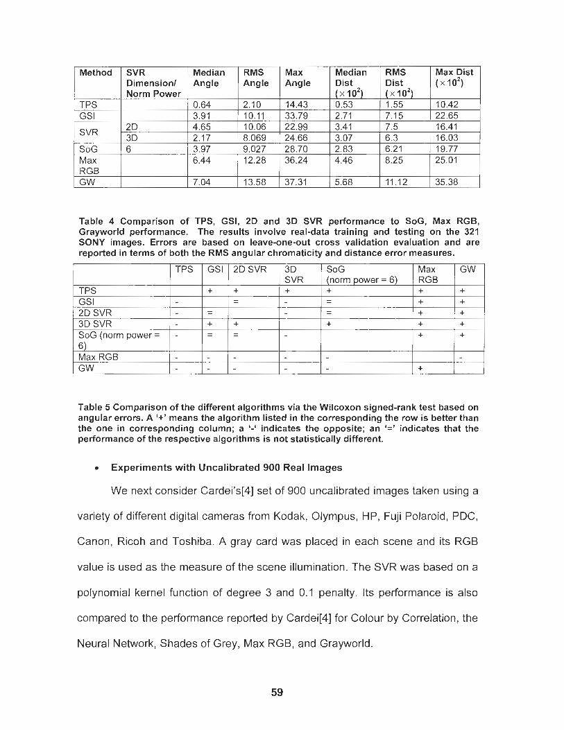
Table 4 Comparison of TPS, GSI, 2D and 3D SVR performance to SoG, Max RGB, Grayworld performance. The results involve real-data training and testing on the 321 SONY images. Errors are based on leave-one-out cross validation evaluation and are reported in terms of both the RMS angular chromaticity and distance error measures.

~ethod-SVR

TPS GSI

SVR

SoG Max RGB GW

Table 5 Comparison of the different algorithms via the Wilcoxon signed-rank test based on angular errors. A '+I means the algorithm listed in the corresponding the row is better than the one in corresponding column; a '-' indicates the opposite; an '=' indicates that the performance of the respective algorithms is not statistically different.

Median Angle

0.64 3.91 4.65 2.17 3.97 6.44

Dimension1 Norm Power

2D 3D 6

Experiments with Uncalibrated 900 Real Images

We next consider Cardei1s[4] set of 900 uncalibrated images taken using a

7.04

variety of different digital cameras from Kodak, Olympus, HP, Fuji Polaroid, PDC,

RMS Angle

2.10 10.11 10.06 8.069 9.027 12.28

Canon, Ricoh and Toshiba. A gray card was placed in each scene and its RGB

13.58

value is used as the measure of the scene illumination. The SVR was based on a

Max Angle

14.43 33.79 22.99 24.66 28.70 36.24

polynomial kernel function of degree 3 and 0.1 penalty. Its performance is also

37.31

compared to the performance reported by Cardei[4] for Colour by Correlation, the

Median Dist ( x loZ) 0.53 2.71 3.41 3.07 2.83 4.46

Neural Network, Shades of Grey, Max RGB, and Grayworld.

5.68

RMS Dist ( x lo2) 1.55 7.1 5 7.5 6.3 6.21 8.25

Max Dist ( x lo2)

1 0.42 22.65 16.41 16.03 19.77 25.01

11.12 35.38

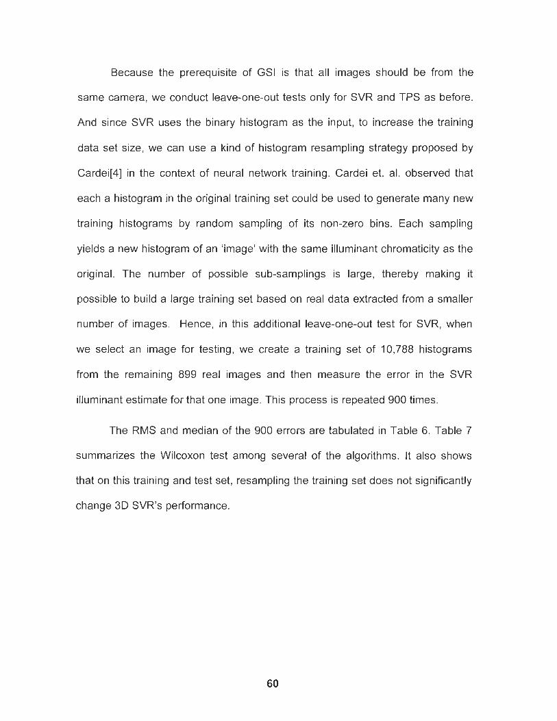
Because the prerequisite of GSI is that all images should be from the

same camera, we conduct leave-one-out tests only for SVR and TPS as before.

And since SVR uses the binary histogram as the input, to increase the training

data set size, we can use a kind of histogram resampling strategy proposed by

Cardei[4] in the context of neural network training. Cardei et. al. observed that

each a histogram in the original training set could be used to generate many new

training histograms by random sampling of its non-zero bins. Each sampling

yields a new histogram of an 'image' with the same illuminant chromaticity as the

original. The number of possible sub-samplings is large, thereby making it

possible to build a large training set based on real data extracted from a smaller

number of images. Hence, in this additional leave-one-out test for SVR, when

we select an image for testing, we create a training set of 10,788 histograms

from the remaining 899 real images and then measure the error in the SVR

illuminant estimate for that one image. This process is repeated 900 times.

The RMS and median of the 900 errors are tabulated in Table 6. Table 7

summarizes the Wilcoxon test among several of the algorithms. It also shows

that on this training and test set, resampling the training set does not significantly

change 3D SVR's performance.

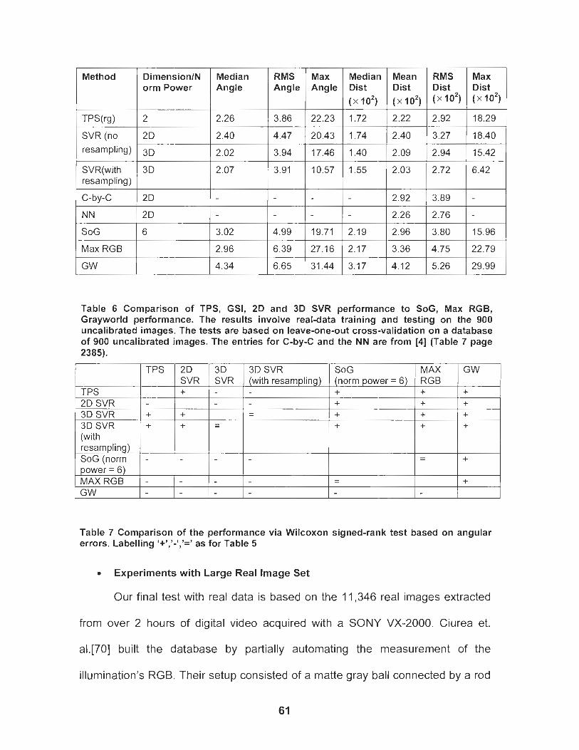
Method / DimensionlN I Median I RMS I Max I Median I Mean I RMS I Max

TPS(rg)

SVR (no resampling)

orm Power

2

2D

3D 1 2.02 1 3.94 1 17.46 1 1.40 1 2.09 1 2.94 1 15.42

SVR(with resampling)

C-by-C

Table 6 Comparison of TPS, GSI, 2D and 3D SVR performance to SoG, Max RGB, Grayworld performance. The results involve real-data training and testing on the 900 uncalibrated images. The tests are based on leave-one-out cross-validation on a database of 900 uncalibrated images. The entries for C-by-C and the NN are from [4] (Table 7 page 2385).

NN

SoG

Max RGB

Angle

2.26

2.40

3D

2D

Table 7 Comparison of the performance via Wilcoxon signed-rank test based on angular errors. Labelling I+','-','=' as for Table 5

2D

6

Experiments with Large Real Image Set

Our final test with real data is based on the 11,346 real images extracted

from over 2 hours of digital video acquired with a SONY VX-2000. Ciurea et.

a1.[70] built the database by partially automating the measurement of the

illumination's RGB. Their setup consisted of a matte gray ball connected by a rod

Angle

3.86

4.47

2.07

TPS 2D SVR 3D SVR 3D SVR (with resampling) SoG (norm power = 6) MAXRGB GW

3.02

2.96

TPS

+ +

-

-

Angle

22.23

20.43

3.91

2D SVR +

+ +

-

4.99

6.39

MAX RGB + + + +

- -

Dist o(io2)

1.72

1.74

10.57

3D SVR

- -

-

GW

+ + + +

+

+

-

19.71

27.16

Dist

pi01 2.22

2.40

1.55

3DSVR (with resampling)

- -

-

-

2.19

2.17

SoG (norm power = 6) + + + +

- -

Dist W o 2 )

2.92

3.27

2.03

2.92

Dist W o 2 )

18.29

18.40

2.26

2.96

3.36

2.72

3.89

6.42

-

2.76

3.80

4.75

-

15.96

22.79

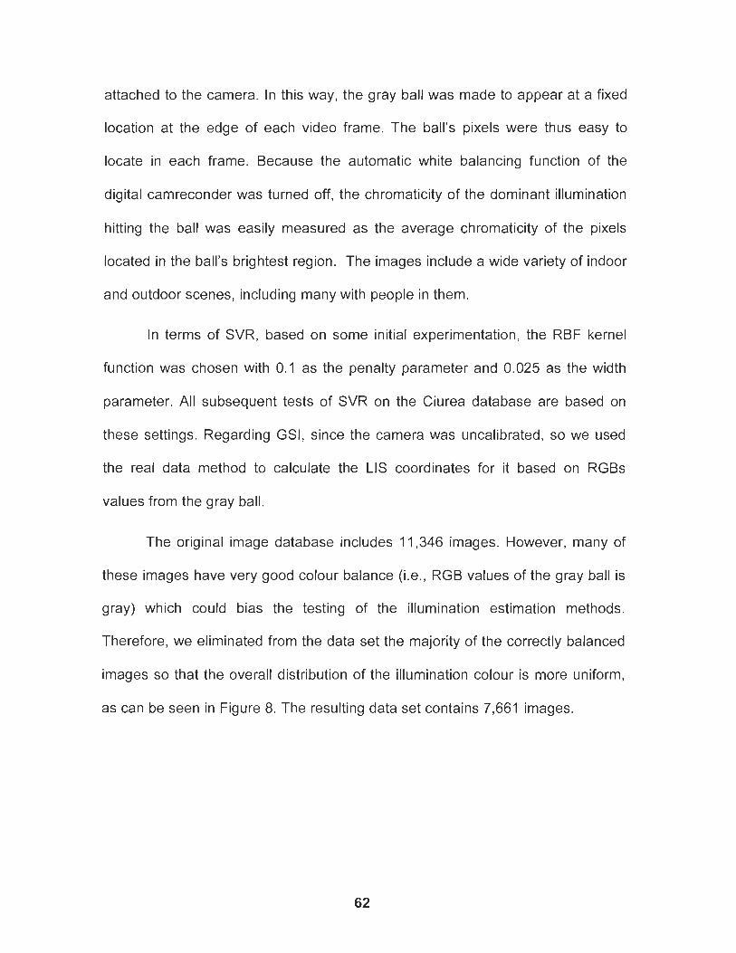
attached to the camera. In this way, the gray ball was made to appear at a fixed

location at the edge of each video frame. The ball's pixels were thus easy to

locate in each frame. Because the automatic white balancing function of the

digital camreconder was turned off, the chromaticity of the dominant illumination

hitting the ball was easily measured as the average chromaticity of the pixels

located in the ball's brightest region. The images include a wide variety of indoor

and outdoor scenes, including many with people in them.

In terms of SVR, based on some initial experimentation, the RBF kernel

function was chosen with 0.1 as the penalty parameter and 0.025 as the width

parameter. All subsequent tests of SVR on the Ciurea database are based on

these settings. Regarding GSI, since the camera was uncalibrated, so we used

the real data method to calculate the LIS coordinates for it based on RGBs

values from the gray ball.

The original image database includes 11,346 images. However, many of

these images have very good colour balance (i.e., RGB values of the gray ball is

gray) which could bias the testing of the illumination estimation methods.

Therefore, we eliminated from the data set the majority of the correctly balanced

images so that the overall distribution of the illumination colour is more uniform,

as can be seen in Figure 8. The resulting data set contains 7,661 images.

Figure 8 (a) The original data set contains 11346 images, but the illumination chromaticities cluster around gray (0.33, 0.33). (b) The reduced data set contains 7661 images with a more uniform distribution of illumination chromaticity.

As shown in Figure 9, the images are cropped to remove the gray ball,

which is located at a fixed location in the lower right quadrant. The resulting

image size is 240 * 240.

Figure 9 (a) Original image containing the gray ball from which the colour of the scene illumination is determined. (b) Cropped image to be used for algorithm testing with gray ball removed.

The size of the database means that leave-one-out validation is not

feasible, although leave-N-out for a reasonable choice of N would be possible. In

any case, it would not necessarily be a fair test because of the inherent

regularities in the database. Since the database was constructed from a 3-frame-

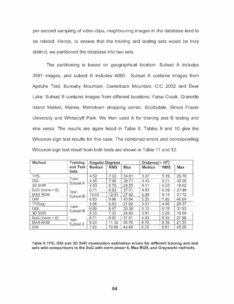
per-second sampling of video clips, neighbouring images in the database tend to

be related. Hence, to ensure that the training and testing sets would be truly

distinct, we partitioned the database into two sets.

The partitioning is based on geographical location. Subset A includes

3581 images, and subset B includes 4080. Subset A contains images from

Apache Trail, Burnaby Mountain, Camelback Mountain, CIC 2002 and Deer

Lake. Subset B contains images from different locations: False Creek, Granville

Island Market, Marine, Metrotown shopping center, Scottsdale, Simon Fraser

University and Whiteclyff Park. We then used A for training and B testing and

vice versa. The results are again listed in Table 8. Tables 9 and 10 give the

Wilcoxon sign test results for this case. The combined errors and corresponding

Wilcoxon sign test result from both tests are shown in Table 11 and 12.

Method

i orm = 6) - -

TPS GSI 3D SVR SoG (norm = 6) MAX RGB GW TPS(rg)

Table 8 TPS, GSI and 3D SVR illumination estimation errors for different training and test sets with comparisons to the SoG with norm power 6, Max RGB, and Grayworld methods.

Training and Test

Angular Degrees I Distancefx I@) Median 1 RMS 1 Max I Median 1 RMS 1 Max

Sets

Train: SubsetA

Test: Subset B

4.52 4.55 4,53 6.71 10.33 6.83

Train: GSI - Subset B

4.58 6.69 -

9.23 7.83

3D SVf -

SoG (n - MAX RGB GW

7.02 7.46 6.76 8.93 12.81 9.66

Test: Subset A

6.83 8.47 7.32 8.92 11.32 10.66

34.81 38.71 24.55 37.01 27.42 43.84 27.62 30.38 24.80 37.01 26.76 43.84

3.37 3.43 4.1 1 4.83 6.99 5.25 3.31 5.12 3.91 4.83 6.76 6.25

5.19 5.71 5.03 6.59 9.14 7.82

25.78 30.26 18.62 27.99 21.72 45.09

4.99 6.78 5.29 6.59 8.39 8.81

29.37 31 -93 16.68 27.99 21.55 45.09

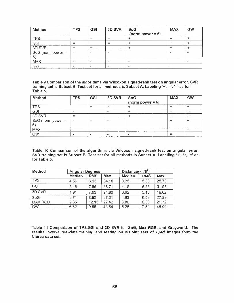
Table 10 Comparison of the algorithms via Wilcoxon signed-rank test on angular error. SVR training set is Subset B. Test set for all methods is Subset A. Labelling I+', I-', '=' as for Table 5.

Table 9 Comparison of the algorithms via Wilcoxon signed-rank test on angular error. SVR training set is Subset B. Test set for all methods is Subset A. Labeling '+', '-', '=' as for Table 5.

MAX

+ + +

+

Method

TPS GS I 3D SVR SOG (norm power = 6) MAX GW

Method

TPS GS I 3D SVR SoG (norm power = 6) MAX GW

GW

+ + + -

GSI

- -

- - -

-

TPS

- - - - =

Method

TPS

TPS

- - -

-

-

Table 11 Comparison of TPS,GSI and 3D SVR to SoG, Max RGB, and Grayworld. The results involve real-data training and testing on disjoint sets of 7,661 images from the Ciurea data set.

3D SVR

- - - -

-

GSI

3D SVR

SoG MAX RGB GW

SoG (norm power = 6)

+ + +

-

GSI

+

+ - -

-

Distance(x ld) Median 1 RMS 1 Max 3.35 1 5.09 1 25.78

Angular Degrees

7.95

7.03

5.46

4.91

Median 4.56

6.71 9.65 6.82

3DSVR

- -

-

RMS 1 Max 6.93 1 34.18

38.71

24.80 8.93 12.13 9.66

SoG (norm power = 6) + - - +

-

4.15

3.62 37.01 27.42 43.84

MAX

+ + + +

- -

6.23

5.16

GW

+ + + +

- -

31.93

18.62 4.83 6.86 5.25

6.59 8.80 7.82

27.99 21.72 45.09

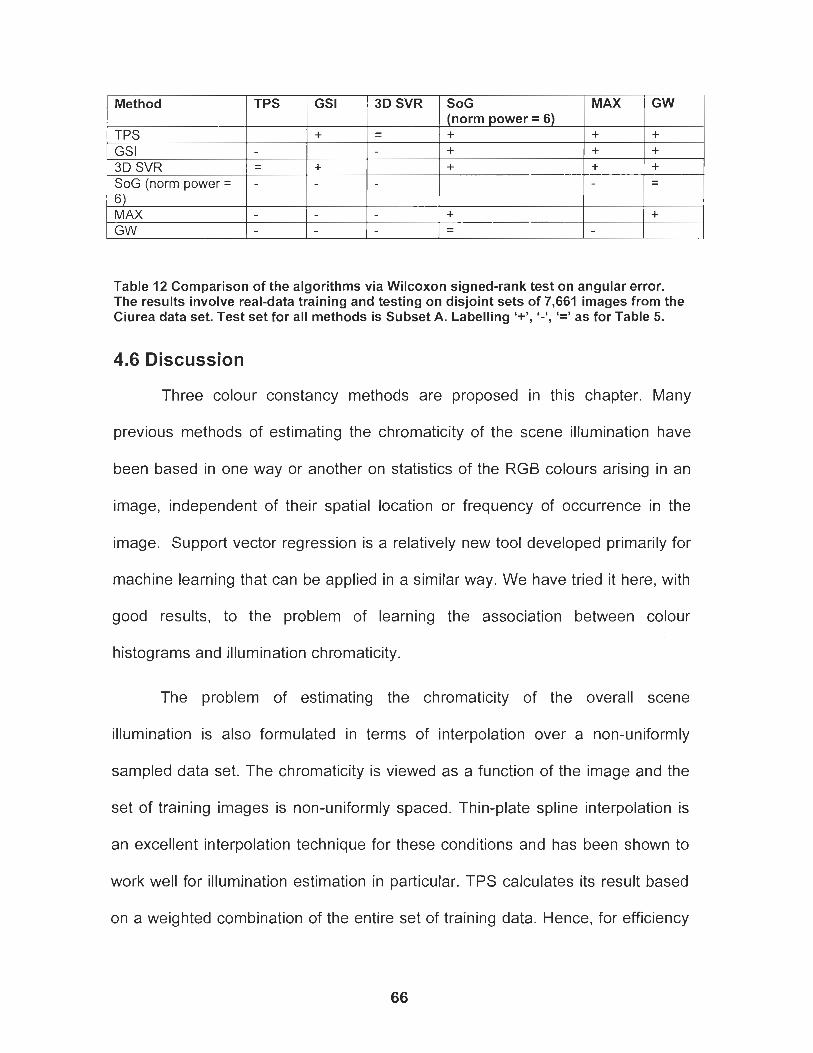
Table 12 Comparison of the algorithms via Wilcoxon signed-rank test on angular error. The results involve real-data training and testing on disjoint sets of 7,661 images from the Ciurea data set. Test set for all methods is Subset A. Labelling I+', I-', '=' as for Table 5.

4.6 Discussion

Three colour constancy methods are proposed in this chapter. Many

MAX

+ + +

Method

TPS GSI 3D SVR SoG (norm power = 6) MAX GW

previous methods of estimating the chromaticity of the scene illumination have

GW

+ + + - -

+

3D SVR

- -

been based in one way or another on statistics of the RGB colours arising in an

SoG (norm power = 6) + + +

+ - -

TPS

- - -

image, independent of their spatial location or frequency of occurrence in the

GSI

+

+

-

image. Support vector regression is a relatively new tool developed primarily for

machine learning that can be applied in a similar way. We have tried it here, with

good results, to the problem of learning the association between colour

histograms and illumination chromaticity.

The problem of estimating the chromaticity of the overall scene

illumination is also formulated in terms of interpolation over a non-uniformly

sampled data set. The chromaticity is viewed as a function of the image and the

set of training images is non-uniformly spaced. Thin-plate spline interpolation is

an excellent interpolation technique for these conditions and has been shown to

work well for illumination estimation in particular. TPS calculates its result based

on a weighted combination of the entire set of training data. Hence, for efficiency

it is important to keep that set as small as possible. Another non-statistical

solution, GSI, is finally proposed that is based on detecting pixels corresponding

to gray surface reflectance--- which is not necessarily the same as gray image

colour--- and using their average image colour as an indicator of the colour of the

overall scene illumination. The gray surfaces are found by first transforming the

image RGB values to a new LIS coordinate system with axes that roughly

correspond to luminance, illumination and reflectance. In LIS coordinates, values

of S near zero tend to be gray. The major advantage of GIs is much faster, does

not require training, and is substantially simpler to implement.

Under almost the same experimentation conditions as those used by

Barnard [ l4 , l5 ] , tests of the shades-of-grey, neural-network, colour-by-

correlation, Max RGB, and Grayworld methods, the experiments show that these

three methods' performance generally is comparable to or better than these other

methods.

All of colour constancy solutions, including the three new ones introduced

in the previous chapter, always assume that there is only one illumination

incident upon the scene. However, this is not true for most typical scenes. The

goal of this chapter is to conduct research on colour constancy under two or

more illuminations. To achieve the goal, the Retinex algorithm for lightness and

colour constancy is extended to include 3-dimensional spatial information

reconstructed from a stereo image. A key aspect of traditional Retinex is that,

within each colour channel, it makes local spatial comparisons of intensity. In

particular, intensity ratios are computed between neighbouring spatial locations.

Retinex assumes that a large ratio indicates a change in surface reflectance, not

a change in incident illumination; however, this assumption is often violated in 3-

dimensional scenes, where an abrupt change in surface orientation can lead to a

significant change in illumination. In this chapter, Retinex is modified to use the

3-dimensional edge information derived from stereo images. The edge map is

used so that spatial comparisons are only made between locations lying on

approximately the same plane in 3-dimensions. Experiments on real images

show this method works well, however, they also reveal that it can lead to

isolated regions, which, as a result of being isolated, are incorrectly determined

1 The chapter also appears as two published papers: Weihua Xiong and Brian Funt, "Stereo Retinex", Third Canadian Conference on Computer and Robot Vision, (Best Vision Paper Award) Quebec, June 2006; Brian Funt and Weihua Xiong, "Colour Space for Stereo Retinex", Third International Conference on Colour in Graphics, Imaging, and Vision, Leeds, June 2006

to be grey. To overcome this problem, stereo Retinex is extended to allow

information that is orthogonal to the space of possible illuminants to propagate

across changes in surface orientation. This is accomplished by transforming the

original RGB image data into the LIS colour space introduced in the last chapter.

This coordinate system allows stereo Retinex to propagate reflectance

information across changes in surface orientation, while at the same time

inhibiting the propagation of potentially invalid illumination information. The

stereo Retinex algorithm builds upon the multi-resolution implementation of

Retinex known as McCann99. Experiments on synthetic and real images show

that stereo Retinex performs significantly better than unmodified McCann99

Retinex when evaluated in terms of the accuracy with which correct surface

object colours are estimated.

5.1 Introduction

Although it is well established that for human subjects, a surface's

perceived spatial location affects the perception of its lightness and colour

[37,41], many machine colour constancy models [l-5,28-361 make no use of 3-

dimensional spatial information. In fact, many of the methods are based on

binarized colour histograms, which discard all the images' spatial structure, and

rely instead on statistical properties of the colour distribution in order to

determine the colour of the scene illuminant. Although these methods work quite

well [14,15], they all assume implicitly that there is a single scene illuminant or a

single adapted illuminant in the visual system. However, multiple illuminants are

common in typical scenes. Outdoors, for example, shadowed areas are not only

darker, but much bluer, than those in the sun, because the sky's light is bluer

than the sun's.

In this chapter, we extend Retinex to take advantage of 3-dimensional

distance information extracted from stereo imagery. In particular, since an abrupt

change in surface orientation may lead to an abrupt change in the incident

illumination as, for example, occurs due to self-shadowing, Retinex is modified so

that its computation does not cross edges in the depth map. In this way, it can

provide lightness/colour estimates for different parts of the scene that may be

illuminated differently.

Although this modification of Retinex does ameliorate many of problems

that arise in multi-illuminant scenes, the processing has a tendency to result in

isolated grey areas. This problem arises especially for surfaces of uniform colour

that are completely isolated from other surfaces by a change in surface

orientation. Retinex normalizes to white, so any completely isolated single colour

will always be made white (or grey after subsequent intensity adjustment). To

overcome this problem, a new colour coordinate system is derived with axes

representing variation in illumination colour, intensity, and object reflectance.

Retinex is applied separately to each of these new colour channels and the result

is then transformed back to the original colour coordinates. The new coordinate

system allows stereo Retinex to propagate reflectance information across

changes in surface orientation, while at the same time inhibiting the propagation

of potentially invalid illumination information.

Tests on synthetic and real images show that the modified, depth-aware

stereo Retinex method outperforms the original Retinex method in terms of the

accuracy with which the true scene surface colours are estimated. Accurate

estimation of scene colours under uncontrolled illumination conditions is

important in many computer vision applications.

5.2 Background

Retinex has a long history beginning with an early paper by Land [22] and

there are many variations on the original Retinex algorithm. We have introduced

them in chapter 3. The basic principles of Retinex are: (i) colour is obtained from

3 'lightnesses' computed separately for each of the colour channels; (ii) the ratios

of intensities from neighbouring locations are assumed to be illumination

invariant; (iii) lightness in a given channel is computed over large regions based

on combining evidence from local ratios; (iv) the location with the highest

lightness in each channel is assumed to have 100% reflectance within that

channel's band. Lightness refers to the perceived (in the case of human

perception), or estimated (in the case of computational methods) surface albedo

(reflectance averaged over the channel's band).

All of the Retinex variants treat the input image as a spatial arrangement

of colours and make no use of the 3-dimensional structure of the underlying

scene. However, there are a number of psychophysical experiments indicating

that the human lightness and colour perception are influenced by information

from several sources, including 3-dimensional scene geometry. In particular,

Gilchrist's early experiments [37] showed that, in the black and white scenes,

changing a surface's apparent 3-dimensional context affected the perception of

its lightness. Gilchrist writes, "The central conclusion of this research is that

perceived surface lightness depends on ratios between regions perceived to lie

next to one another in the same plane."[37]. The extension to Retinex proposed

here uses ratios between regions lying next to one another and, furthermore,

specifically excludes ratios from neighbouring regions lying in different planes. In

experiments using computer graphics rendered 3-dimensional scenes, Boyaci

et.al. [40] provided further evidence for the relationship between perceived

orientation and the perceived lightness of matte surfaces. Yamauchi and

Uchikawa 1361 used stereoscopic stimuli to support the notion that surface colour

perception is strongly influenced by depth information. Bloj et.al. 1721 illustrated

the effect of spatial shape on chromatic recognition. Yang and Shevell 1391 show

that binocular disparity can improve colour constancy. Adelson 1731 argues that

statistical properties and spatial arrangement in three dimensions are combined

for lightness perception.

Since there is plenty of psychophysical evidence indicating a connection

between a surface's spatial properties in 3-dimensions and its perceived

lightness and colour properties, the question is how to include the spatial

information into a colour constancy model? We investigate how it can be

incorporated into the Retinex model in particular, and show that spatial

information does improve its colour constancy performance significantly.

5.3 Stereo Retinex Basics

Since we begin with the multi-resolution version of the Retinex algorithm,

known as McCann99 [23], and extend it to include 3D spatial information, we

briefly describe the original algorithm. McCann99 is a multi-resolution technique

which involves the standard pyramid of decreasing resolution. The computation

starts at the top of the pyramid with a ratio-product-reset-average process that

involves local comparisons between each pixel and its immediate neighbors. The

procedure is iterative so that a pixel's lightness estimate is updated based on its

current lightness estimate in conjunction with its intensity ratios with respect to its

neighbors. After a fixed, but user-selectable, number of iterations, the lightness

estimates are propagated down a layer where the computation is continued, then

propagated further.

We use a stereo image to calculate a depth map registered with the image

data. Details of the camera setup, calibration and stereo-correspondence

algorithm will be described in the Experiments section; however, any standard

stereo-reconstruction algorithm could be used. Edges in the depth map are then

detected using a modified version of the method proposed by Gelautz et.al [74].

These edges represent sharp changes in surface orientation, or depth

discontinuities such as those created by occlusion.

The depth edges are the key factor in controlling the spatial comparisons

made during the Retinex computation. Traditional Retinex compares a pixel to all

its neighbors. In this case, the implicit assumption is that a large change in

intensity between pixels arises from a change in surface reflectance, while a

small change arises from a gradual change in illumination. However, in 3-

dimensions an abrupt change in surface orientation can also mean that there is

an abrupt change in the incident illumination, since the differently oriented parts

of the surface may be pointed towards different light sources. Similarly, depth

discontinuities imply that there are two separate surfaces, which may, of course,

be illuminated differently. As Gilchrist [37] pointed out, the only spatial

comparisons between neighboring locations on the same locally planar surface

should be used. With the additional information about the location of depth edges

derived from stereo, the proposed stereo Retinex method only makes

comparison between pixels that do not cross a depth edge. Although this is

conceptually simple, the computation requires some organization, especially to

accommodate the multi-resolution aspect of McCann99 Retinex.

Since McCann99 Retinex compares values at neighboring pixels and

averages lightness estimates from them as well, what is required is an efficient

way to stop it making comparisons across depth edges. This is accomplished by

first constructing separate maps for vertical and horizontal edges elements. This

division makes it easier to propagate the edges up to lower resolution levels of

the multi-resolution pyramid. Once the edge information is propagated through

the pyramid, a bit-mask is used to encode the subset of the immediate a pixel's 8

neighbors that are all on the same side of any edges. As McCann99 iterates, it

simply uses the bit-mask encoding to determine which neighbors to visit. Details

are given below in the "Implementation Details" section.

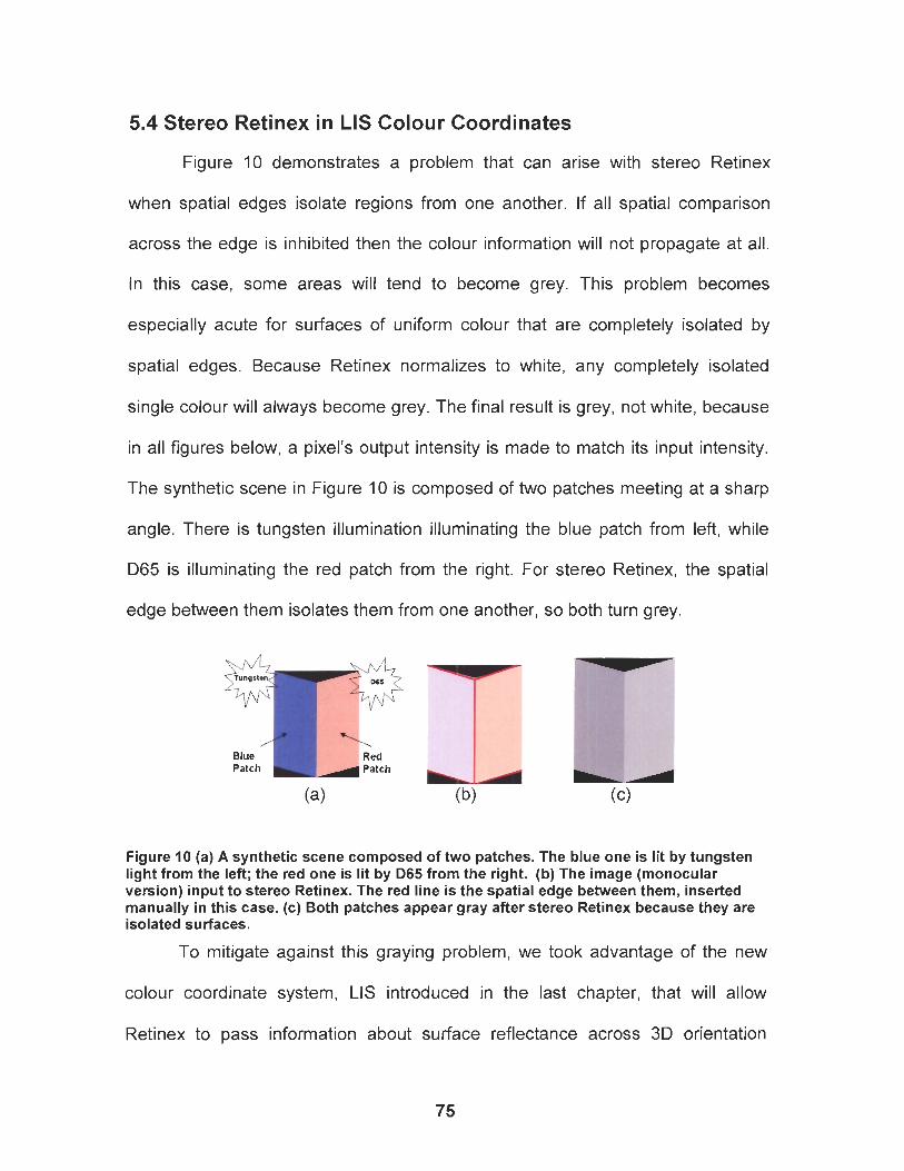
5.4 Stereo Retinex in LIS Colour Coordinates

Figure 10 demonstrates a problem that can arise with stereo Retinex

when spatial edges isolate regions from one another. If all spatial comparison

across the edge is inhibited then the colour information will not propagate at all.

In this case, some areas will tend to become grey. This problem becomes

especially acute for surfaces of uniform colour that are completely isolated by

spatial edges. Because Retinex normalizes to white, any completely isolated

single colour will always become grey. The final result is grey, not white, because

in all figures below, a pixel's output intensity is made to match its input intensity.

The synthetic scene in Figure 10 is composed of two patches meeting at a sharp

angle. There is tungsten illumination illuminating the blue patch from left, while

D65 is illuminating the red patch from the right. For stereo Retinex, the spatial

edge between them isolates them from one another, so both turn grey.

/

Blue \

Red I Patch , Patch

(a> 41

(b)

Figure 10 (a) A synthetic scene composed of two patches. The blue one is lit by tungsten light from the left; the red one is lit by D65 from the right. (b) The image (monocular version) input to stereo Retinex. The red line is the spatial edge between them, inserted manually in this case. (c) Both patches appear gray after stereo Retinex because they are isolated surfaces.

To mitigate against this graying problem, we took advantage of the new

colour coordinate system, LIS introduced in the last chapter, that will allow

Retinex to pass information about surface reflectance across 3D orientation

changes while still inhibiting the exchange of possibly incorrect illumination

information. Since LIS can represent illumination change, reflectance and

luminance as an independent component as possible, the basic stereo Retinex

method described above is modified so that, at a 3D surface edge, information is

allowed to propagate within the channel representing surface reflectance, while it

continues to be inhibited within the illumination and intensity channels.

5.5 Implementation Details

The main difficulty in implementing stereo Retinex as a modification of the

McCann99 algorithm is in transmitting the spatial edge information from one level

of the multi-resolution pyramid to the next. For convenience, the edges found

from the stereo depth map are assumed to lie in between image pixels. To

propagate the edge information to the next lower resolution level in the pyramid,

the rewrite rules shown in Figure 11 are used. For a 2-by-2 group of pixels, if

they are all to one side of an edge then the edge is easily propagated to the next

level. For the case where a vertical edge runs through the group, it is randomly

assigned to pass on one side of the group or the other; or above or below it in the

case of a horizontal edge.

Case 1 No Edges Case 2 One Edge Element

a I3 Random

Case 3 Two Edge Elements

a bN Random

Figure 11 Rewrite rules using in propagating edge information to the next lower resolution. An edge running through the middle of a 2-by-2 region is randomly assigned to one side or the other. Vertical edges are shown here. Horizontal edges are treated analogously.

If there are any edges between a pixel and its neighbors, then it should

only make comparisons with a subset of those neighbors. This subset is

compactly represented by the 'on' bits in an 8-bit mask using 1 bit for each of a

pixel's 8 immediate neighbors. This strategy is useful for reducing the memory

requirements. Deciding whether or not an edge must be crossed to reach a

neighbor to the east, south, west, or north is straightforward because the edges

are either above or to the side of a pixel. For a diagonal neighbor, the one to the

northeast for example, an edge must be crossed if there are edges both to the

north and to the east. Together they surround the pixel's northeast corner

forming an edge as shown in Figure 12a. Similarly, an edge must be crossed to

reach either of the 2 shaded pixels in Figure 12b.

Figure 12 (a) From the center pixel, the three shaded pixels in the upper right can not be reached without crossing an edge. (b) The two pixels that can not be reached are shaded.

At each iteration, McCann99 compares each pixel to its neighbors and

averages the local lightness estimates. The algorithm is modified to use the 8-bit

neighbor mask to indicate what subset of the neighbors to use. The number of

'on' bits also indicates the number to divide by in the averaging step.

For stereo matching, we use a fast cross-correlation, rectangular sub-

regioning, and 3D maximum-surface techniques in a coarse-to-fine scheme [75].

However, noise in the image, as well as errors in calibration and rectification, can

lead to false matches being made that lead to errors in the depth map. To

improve the accuracy of detected spatial edges, we use the 'edge combination'

technique developed by Gelautz et-al [74]. We used their original method with the

exception of using Laplacian of Gaussian edge detection in place of Canny

detection, since for our purposes it seemed to give slightly better results.

5.6 Experiments

We implemented stereo Retinex in Matlab 7.0 by downloading and

modifying the McCann99 Matlab code available from the Simon Fraser University

Computational Vision Laboratory [65]. We then tested it on both synthetic and

real images. Retinex's performance is evaluated in terms of the accuracy with

which it estimates the chromaticity of surface colours as they would occur under

a canonical 'white' illumination.

Images were captured using a Kodak DCS460 single-lens reflex digital

camera. A "LORE0 3D lens in a cap" is attached in place of the standard lens so

that the camera records a stereo pair within a single image frame[76]. Camera

geometry calibration, image rectification and stereo matching were conducted

using standard procedures [69,71]. We use the stereo image to calculate a 3D

depth map and then detect edges in the depth map using a modified version of

the method proposed by Gelautz et.al [74].

We evaluate performance in terms of the distance between colours in rg-

chromaticity (r=R/(R+G+B), g=G/(R+G+B)) space, and in terms of the angle

between colours viewed as vectors in RGB space. These are given by the

following formulas, where subscript 'el indicates the result of Retinex processing,

and 'w' indicates the 'benchmark' colour under white light:

We report four basic statistical measures of the error distributions: mean,

median, RMS (root mean square) and Mmax. Mmax is the average value of the

largest p percent of the errors. Mmax is more stable with respect to presence of

an isolated extreme value than the simple maximum. In this paper, p is set to be

0.5 practically. Hordley et. al. [67] indicate that the median angular error is often

the most appropriate one to use when evaluating colour constancy. RMS of the

errors from N pixels is given by the standard formula:

5.6.1 Tests using synthetic images

Since stereo reconstruction and edge detection will be imperfect, one goal

of the synthetic-image tests is to determine how much undetected edges will

affect accuracy. It is also useful to compare the performance of stereo Retinex to

McCann99 Retinex in a controlled, noise-free environment, with ground-truth

data for the colours of the objects in the scene.

The synthetic images are constructed with a variable number of patches of

different reflectances selected from the 1995 available in the database described

by Barnard 1651. The illumination spectrum and sensor sensitivity functions 1681 of

a SONY DXC-930 3-CCD camera are used to derive the RGB for each patch.

First, a benchmark image is generated using equal-energy white illumination.

Second, using the same patch reflectances, the same synthetic scene is divided

into two parts. RGB1s for one part are synthesized using the spectrum of

tungsten light, and for the-other using D65 daylight. All the reflectance and

illuminant data were downloaded from the Simon Fraser University colour

database 1651. For the synthetic case, we do not synthesize stereo images, but

instead create the depth-edge map manually so that the number and extent of

leaks between the two differently illuminated parts of the image can be

controlled.

For the first experiment, we divided the image down the middle. We apply

stereo Retinex to the image once providing it a perfect edge map. The results are

shown visually in Figure 13 and tabulated numerically in Table 13.

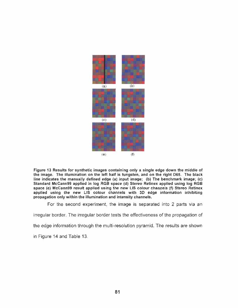
Figure 13 Results for synthetic images containing only a single edge down the middle of the image. The illumination on the left half is tungsten, and on the right D65. The black line indicates the manually defined edge (a) Input image; (b) The benchmark image; (c) Standard McCann99 applied in log RGB space (d) Stereo Retinex applied using log RGB space (e) McCann99 result applied using the new LIS colour channels (f) Stereo Retinex applied using the new LIS colour channels with 3D edge information inhibiting propagation only within the illumination and intensity channels.

For the second experiment, the image is separated into 2 parts via an

irregular border. The irregular border tests the effectiveness of the propagation of

the edge information through the multi-resolution pyramid. The results are shown

in Figure 14 and Table 13.

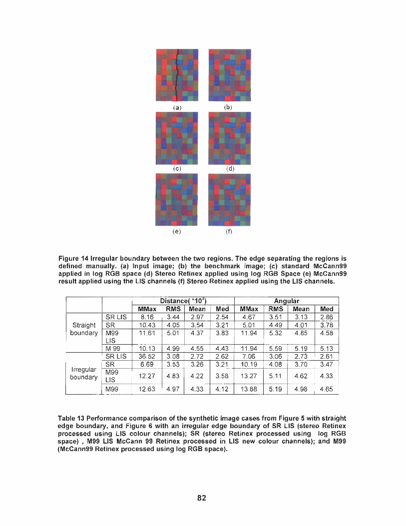
Figure 14 Irregular boundary between the two regions. The edge separating the regions is defined manually. (a) Input image; (b) the benchmark image; (c) standard McCann99 applied in log RGB space (d) Stereo Retinex applied using log RGB Space (e) McCann99 result applied using the LIS channels (f) Stereo Retinex applied using the LIS channels.

Table 13 Performance comparison of the synthetic image cases from Figure 5 with straight edge boundary, and Figure 6 with an irregular edge boundary of SR LIS (stereo Retinex processed using LIS colour channels); SR (stereo Retinex processed using log RGB space) , M99 LIS McCann 99 Retinex processed in LIS new colour channels); and M99 (McCann99 Retinex processed using log RGB space).

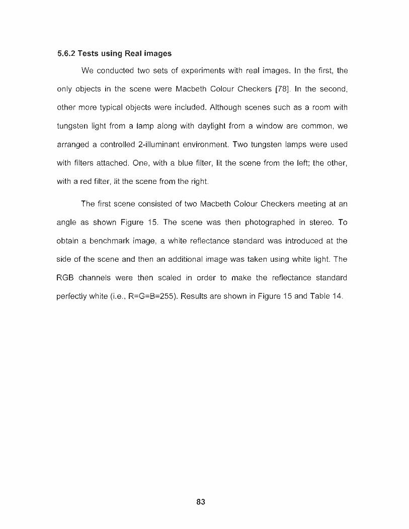
5.6.2 Tests using Real images

We conducted two sets of experiments with real images. In the first, the

only objects in the scene were Macbeth Colour Checkers [78]. In the second,

other more typical objects were included. Although scenes such as a room with

tungsten light from a lamp along with daylight from a window are common, we

arranged a controlled 2-illuminant environment. Two tungsten lamps were used

with filters attached. One, with a blue filter, lit the scene from the left; the other,

with a red filter, lit the scene from the right.

The first scene consisted of two Macbeth Colour Checkers meeting at an

angle as shown Figure 15. The scene was then photographed in stereo. To

obtain a benchmark image, a white reflectance standard was introduced at the

side of the scene and then an additional image was taken using white light. The

RGB channels were then scaled in order to make the reflectance standard

perfectly white (i.e., R=G=B=255). Results are shown in Figure 15 and Table 14.

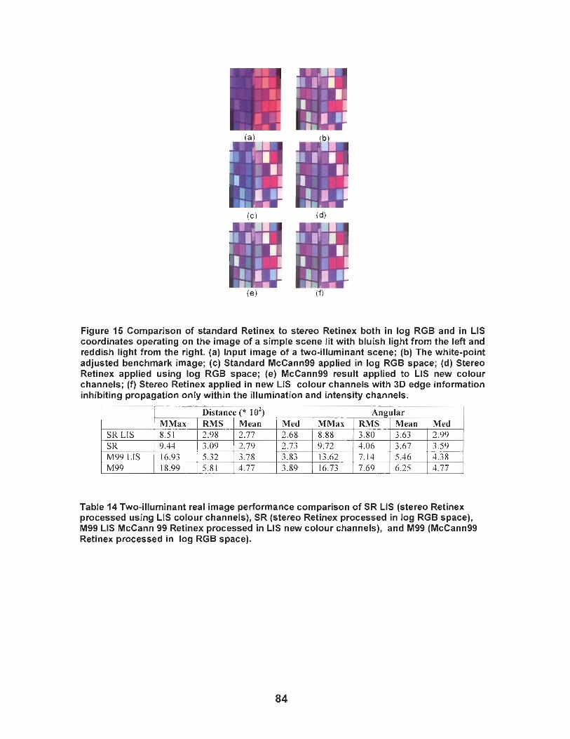
Figure 15 Comparison of standard Retinex to stereo Retinex both in log RGB and in LIS coordinates operating on the image of a simple scene lit with bluish light from the left and reddish light from the right. (a) Input image of a two-illurninant scene; (b) The white-point adjusted benchmark image; (c) Standard McCann99 applied in log RGB space; (d) Stereo Retinex applied using log RGB space; (e) McCann99 result applied to LIS new colour channels; (f) Stereo Retinex applied in new LIS colour channels with 3D edge information inhibiting propagation only within the illumination and intensity channels.

Table 14 Two-illuminant real image performance comparison of SR LIS (stereo Retinex processed using LIS colour channels), SR (stereo Retinex processed in log RGB space), M99 LIS McCann 99 Retinex processed in LIS new colour channels), and M99 (McCann99 Retinex processed in log RGB space).

Angular MMar I RMS 1 Mean ] Med 8.88 1 3.80 1 3.63 1 2.99 SR LIS

Distance (* lo2) lMMax 1 RMS 1 Mean 1 ~Med 8.5 1 1 2.98 1 2.77 1 2.68

Figure 16 Edge map and recovered illumination: (a) Edges representing abrupt changes in surface orientation extracted from the stereo image pair are marked in white; (b) Chromaticity of illumination as estimated by stereo Retinex in LIS colour channels correctly shows a sharp change in illumination where the surface orientation changes; (c) Illumination field recovered by McCann99 shows a much less distinct change in illumination.

The surface orientation edge in the previous scene is very distinct and

easily identified. To test how well stereo Retinex works in a less controlled

environment, we use the more complex scenes shown in Figures 17 and 18.

Again, Figure 17 has blue light from the right and red light from the left. As can

be seen from the white bust in the upper right, as well as the white button in the

lower left, stereo Retinex in log RGB (Fig. 17 (e)) is more successful at

eliminating the illumination variation than McCann99 (Fig. 17 (d)). Both methods

push the colours towards grey because Retinex normalizes colours relative to the

whitest surface within a local region. This leads to desaturation of the colours

when there is no nearby white surface. In the case of stereo Retinex, this

problem is exacerbated by the fact that depth edges (correctly) limit the distance

within which a white surface needs to be found. Using the new LIS colour space,

more surface colour information propagates across the edges and this leads to

the more colorful result Fig. 17 (g).

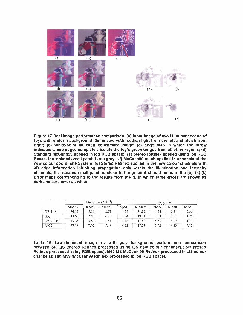
Figure 17 Real image performance comparison. (a) Input image of two-illuminant scene of toys with uniform background illuminated with reddish light from the left and bluish from right; (b) White-point adjusted benchmark image; (c) Edge map in which the arrow indicates where edges completely isolate the toy's green tongue from all other regions; (d) Standard McCann99 applied in log RGB space; (e) Stereo Retinex applied using log RGB Space, the isolated small patch turns gray; (f) McCann99 result applied to channels of the new colour coordinate System; (g) Stereo Retinex applied in the new colour channels with 3D edge information inhibiting propagation only within the illumination and intensity channels, the isolated small patch is close to the green it should be as in the (b). (h)-(k) Error maps corresponding to the results from (d)-(g) in which large errors are shown as dark and zero error as white

Table 15 Two-illuminant image toy with gray background performance comparison between SR LIS (stereo Retinex processed using LIS new colour channels); SR (stereo Retinex processed in log RGB space), M99 LIS McCann 99 Retinex processed in LIS colour channels); and M99 (McCann99 Retinex processed in log RGB space).

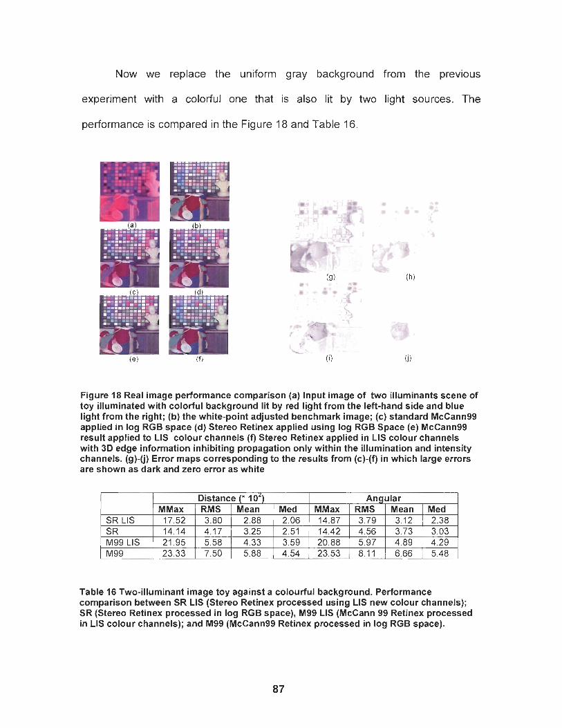
Now we replace the uniform gray background from the previous

experiment with a colorful one that is also lit by two light sources. The

performance is compared in the Figure 18 and Table 16.

Figure 18 Real image performance comparison (a) Input image of two illuminants scene of toy illuminated with colorful background lit by red light from the left-hand side and blue light from the right; (b) the white-point adjusted benchmark image; (c) standard McCann99 applied in log RGB space (d) Stereo Retinex applied using log RGB Space (e) McCann99 result applied to LIS colour channels (f) Stereo Retinex applied in LIS colour channels with 3D edge information inhibiting propagation only within the illumination and intensity channels. (9)-(j) Error maps corresponding to the results from (c)-(f) in which large errors are shown as dark and zero error as white

M99 LIS 1 21.95 1 5.58 1 4.33 1 3.59 1 20.88 1 5.97 1 4.89 1 4.29 M99 1 23.33 1 7.50 1 5.88 1 4.54 1 23.53 1 8.11 1 6.66 1 5.48

SR LIS SR

Table 16 Two-illuminant image toy against a colourful background. Performance comparison between SR LIS (Stereo Retinex processed using LIS new colour channels); SR (Stereo Retinex processed in log RGB space), M99 LIS (McCann 99 Retinex processed in LIS colour channels); and M99 (McCann99 Retinex processed in log RGB space).

Distance (* 10') MMax

17.52 14.14

Angular MMax 14.87 14.42

RMS 3.80 4.17

RMS 3.79 4.56

Mean 2.88 3.25

Med 2.06 2.51

Mean 3.12 3.73

Med 2.38 3.03

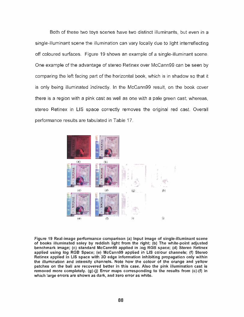
Both of these two toys scenes have two distinct illuminants, but even in a

single-illuminant scene the illumination can vary locally due to light interreflecting

off coloured surfaces. Figure 19 shows an example of a single-illuminant scene.

One example of the advantage of stereo Retinex over McCann99 can be seen by

comparing the left facing part of the horizontal book, which is in shadow so that it

is only being illuminated indirectly. In the McCann99 result, on the book cover

there is a region with a pink cast as well as one with a pale green cast; whereas,

stereo Retinex in LIS space correctly removes the original red cast. Overall

performance results are tabulated in Table 17.

Figure 19 Real-image performance comparison (a) Input image of single-illuminant scene of books illuminated soley by reddish light from the right; (b) The white-point adjusted benchmark image; (c) standard McCann99 applied in log RGB space; (d) Stereo Retinex applied using log RGB Space; (e) McCann99 applied in LIS colour channels; (f) Stereo Retinex applied in LIS space with 3D edge information inhibiting propagation only within the illumination and intensity channels. Note how the colour of the orange and yellow patches on the ball are recovered better in this case. Also the pink illumination cast is removed more completely. (9)-(j) Error maps corresponding to the results from (c)-(f) in which large errors are shown as dark, and zero error as white.

Table 17 Single-illuminant real image books scene performance comparison between SR LIS (stereo Retinex processed using LIS new colour channels); SR (stereo Retinex processed in log RGB space), M99 LIS McCann 99 Retinex processed in LIS space); and M99 (McCann99 Retinex processed in log RGB space).

5.7 Retinex's iteration parameter

One of the key parameter choices to make when running McCann99

Retinex is the number iterations to be conducted at each pyramid level. The

larger the number of iterations the greater distance at which pixels affect one

another. Figure 20 plots the median chromaticity angular error as a function of

the number of iterations for the scene from Figure 18. The plots for all the other

scenes showed a similar trend. From this plot, it appears that 1 iteration is the

best choice, so it is what has been used to obtain all the results reported above.

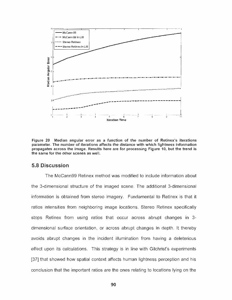
- McCann 99

-.- McCann 99 in LIS

m m m a - Stereo Retinex

- -- Stereo Retinex In LIS

i I I I I I I I I I 2 3 4 5 6 7 8 9 10

Iteration Time

Figure 20 Median angular error as a function of the number of Retinex's iterations parameter. The number of iterations affects the distance with which lightness information propagates across the image. Results here are for processing Figure 10, but the trend is the same for the other scenes as well.

5.8 Discussion

The McCann99 Retinex method was modified to include information about

the 3-dimensional structure of the imaged scene. The additional 3-dimensional

information is obtained from stereo imagery. Fundamental to Retinex is that it

ratios intensities from neighboring image locations. Stereo Retinex specifically

stops Retinex from using ratios that occur across abrupt changes in 3-

dimensional surface orientation, or across abrupt changes in depth. It thereby

avoids abrupt changes in the incident illumination from having a deleterious

effect upon its calculations. This strategy is in line with Gilchrist's experiments

[37] that showed how spatial context affects human lightness perception and his

conclusion that the important ratios are the ones relating to locations lying on the

same 3-space plane. Although stereo imagery was used here to determine the 3-

dimensional structure, any other method (e.g. from shading in a monocular

image) of identifying when neighbouring image pixels correspond to scene points

lying on a locally planar surface would work just as well.

Although a significant improvement over traditional Retinex, stereo

Retinex also highlights the problem that limiting the propagation of lightness

information across the image increases the likelihood that it will normalize

colours relative to a colour which is not a true white, with the result that some

colours are estimated as being more desaturated than they should be. To solve

this problem, the new colour coordinate system, LIS, was again introduced for

use in Retinex processing. The new coordinate system defines channels that

relate to changes in illumination, intensity and reflectance. Both Retinex and

stereo Retinex applied to these channels performs modestly better than when

either is applied to the standard log RGB channels. By at least partially

separating changes in surface reflectance from changes in illumination and

intensity, the LIS colour space makes it possible to express the fact that across

an abrupt change in 3D surface orientation the comparison of surface reflectance

information across the edge remains valid even though the illumination may have

changed in unpredictable ways

Stereo Retinex outperforms McCann99 Retinex in its ability to estimate

the chromaticity of surface colours as they would appear under ideal white light.

For the case of Retinex at least, this demonstrates that knowledge of scene's 3-

dimensional spatial structure can be useful for colour constancy.

CHAPTER 6: COLOUR CONSTANCY FOR MULTIPLE- ILLUMINANT SCENES USING RETINEX AND SVR'

Scenes lit by multiple colours of illumination provide a problem for colour

constancy and automatic white balancing algorithms. Many of these algorithms

estimate a single illuminant colour, but when there are multiple illuminants, there

is in fact not a single correct answer when we recover the surface reflectance.

For automatic white balancing and colour-cast removal in digital images, multiple

illuminants mean that a single, image-wide adjustment of colours may not yield a

good result, since the adjustment that makes one image area look better, may

simultaneously make another look worse. Retinex is one method that adjusts

colours on a pixel-by-pixel basis, and so inherently addresses the multiple-

illumination problem, but it does not always produce a perfect overall colour

balance. In the last chapter, we tried to solve the problem by extending Retinex

with 3D spatial information. However, Stereo Retinex requires two or more

images captured simultaneously from different view points, which is not practical.

On the other hand, illumination estimation by Support Vector Regression (SVR),

produces quite good overall colour balance for single-illuminant scenes, but does

not adjust the colours locally. Therefore, in this chapter, we combine Retinex and

SVR into a hybrid Retinex+SVR method to overcome some of these problems.

Experiments with both synthetic and real images show promising results.

1 This chapter also appears as a published paper: Weihua Xiong and Brian Funt, "Colour Constancy for Multiple-llluminant Scenes using Retinex and SVR,", in Proc, of Imaging Science and Technology Fourteenth Colour Imaging Conference pp. 304-308, Nov. 2006

6.1 Introduction

Many scenes involve multiple sources of illumination. One very common

example occurs when one is indoors and looks across the room and through a

window to the outdoors. The indoor illumination will generally be reddish in

comparison to the bluish illumination provided by the sky. These situations can

lead to very strange output. If the camera is correctly balanced for the indoor

illumination, the window will often look far too blue. The problem is that a single

colour balance setting is insufficient. The colours must, to some extent at least,

be adjusted locally to account for the local variation in scene illumination.

The majority of the illumination-estimation methods [I-5,28-361 that have

been developed for automatically colour balancing images makes a single

estimate of the scene illumination. They, therefore, are susceptible to the

situations such as the too blue window. Retinex is an exception in that it makes

a separate illumination estimate for each pixel. Although this is strength of

Retinex, it can also be a weakness in that the illumination estimate is strongly

influenced by the colours in each pixel's neighbourhoods. For pixels that have

same initial colour values but are at very different locations, Retinex's output may

be different.

Our goal is to gain the benefits of both the local and global approaches by

merging them into a single process. In particular, we use Retinex to make local

colour adjustments and then apply the Support Vector Regression (SVR) method

to the Retinex-processed image to adjust the overall colour balance. In scenes

with strong differences of illumination, our hypothesis is that because it makes

local adjustments, Retinex will attenuate the differences in illumination, and as

result SVR will be able to make a better global adjustment for the illumination.

The experiments describe below show that this hybrid method works better than

either SVR or Retinex alone.

6.2 Implementation Details

For the Retinex implementation, we use the Matlab version of McCann99

Retinex [66] . For Support Vector Regression we use the "3D" method described

in chapter 4 which is based on binarized histograms of the image pixels' (L, r, g)

where L = R + G + B and r=R/L and g = G/L. We quantize L into 25 equal steps,

and r and g into 50 steps so the 3D histograms consist of 62,500 (25x50~50)

bins. After training, SVR provides an estimate of the rg-chromaticity of the overall

scene illumination based on the binarized image histogram submitted to it.

SVR requires a training set. We created a training set of 56,730

histograms by random subsampling of colours from images contained in the

11,346 "grayball" image database [70].

Each image is processed first with McCann99 Retinex. The binarized Lrg

colour histogram of the resulting image is then passed to SVR which returns the

estimate of the illumination chromaticity. The SVR estimate is not actually an

estimate of the true illumination, but rather an estimate of the illumination relative

to the post-Retinex-processed image. The SVR illumination estimate is used in a

diagonal von Kries transformation to correct the post-Retinex image in order to

adjust it to have the colours it would have had if the original scene had been

imaged under the canonical illumination. This Retinex-SVR image is then

compared with the ground-truth image of the same scene imaged under the

canonical white illumination

We evaluate Retinex-SVR performance at each pixel in terms of the

distance between measured in rg-chromaticity (r=R/(R+G+B), g=G/(R+G+B))

space and in terms of the angle in degrees between colours in RGB space.

These errors are defined by the following formulas, where subscript 'p' indicates

the result after Retinex-SVR and 'g' indicates the ground-truth image.

We also compute three statistics on the distribution of errors across all the

pixels in an image: the median, the RMS (root mean square) and the mean of

the top 112 percentile of the largest errors, denoted MMax. In contrast to a single

maximum error, MMax is a more representative measure of the methods failures.

RMS of the errors from N pixels is given by the standard formula:

The Wilcoxon signed-rank test based on angular error with a 0.01

threshold for accepting or rejecting the null hypothesis is also used to evaluate

difference between error distributions [67].

6.2.1 Synthetic Image Experiments

Our first experiments are based on synthetic images that model a scene

with two quite distinct illuminants lighting different parts of the scene. We

generate synthetic scenes composed of patches of different reflectance by

randomly selecting reflectances from the 1995 available in the database

described by Barnard [65]. The patches are divided into two sections by an

irregular boundary representing where the illumination changes. RGB values for

the patches are calculate by using two illumination spectra, CIE A on the left, CIE

D65 daylight on the right, and sensor sensitivity functions of the SONY DXC-930

camera colour balanced equal-energy white. The ground-truth image is

generated using equal-energy white illumination over the whole scene. The

sensitivity functions were normalized for this white light. All of the spectra and

sensitivity functions were downloaded from the Simon Fraser University colour

database [69].

Figure 21 shows the results of SVR, Retinex and Retinex+SVR

processing. The top left Mondrian is the input image with a white line

superimposed demarcating the boundary between the two illuminations to make

it easier to see. The line is not part of the actual input image. SVR applied to the

input Mondrian estimates the illumination's rgb-chromaticity as [0.375, 0.298,

0.3081, in other words, as quite reddish in comparison to white [0.333, 0.333,

0.3331. This successfully removes some of the reddish cast from the left side of

the image, but introduces more blue to the right side (Figure 21, bottom row on

the left). On the other hand, when SVR is applied to the Retinex-processed

image (Figure 21, middle row on the left), it estimates the "illumination" as a

bluish [0.296, 0.31 5, 0.3891. In this second case, there was no actual illumination;

rather it is SVR's estimate of what the illumination would be if the Retinex output

were actually an unprocessed input image. Since the Retinex result is too blue in

comparison to the ground-truth Mondrian (top right), correcting the colours based

on SVR's estimate improves the image so that now the bottom right

(Retinex+SVR) and top right (ground truth) images are very similar. Numerical

results are tabulated in Tables 18 and 19. The Wilcoxon signed-rank test applied

to the angular error indicates that for this image the performance difference is

significant and that Retinex+SVR outperforms Retinex, and Retinex outperforms

SVR.

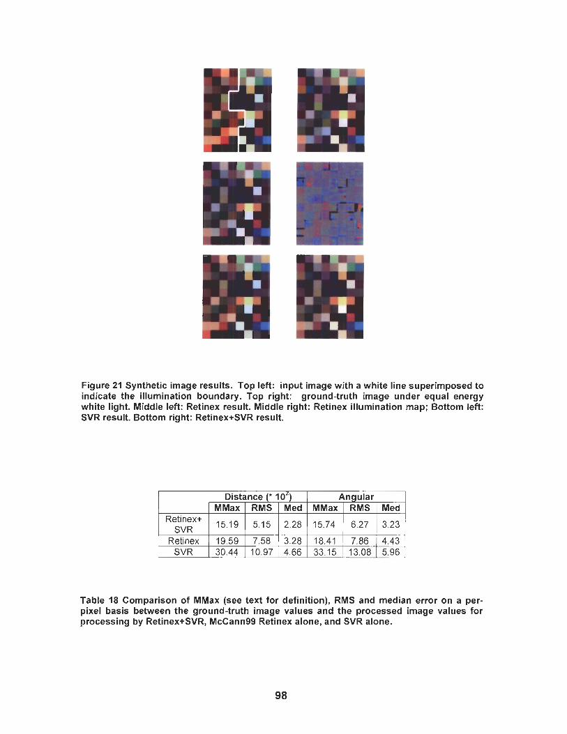
Figure 21 Synthetic image results. Top left: input image with a white line superimposed to indicate the illumination boundary. Top right: ground-truth image under equal energy white light. Middle left: Retinex result. Middle right: Retinex illumination map; Bottom left: SVR result. Bottom right: Retinex+SVR result.

1 Distance (* l o L ) I Anaular

Retinex 1 19.59 / 7.58 1 3.28 1 18.41 1 7.86 1 4.43 SVR 1 30.44 1 10.97 / 4.66 1 33.15 / 13.08 1 5.96

Table 18 Comparison of MMax (see text for definition), RMS and median error on a per- pixel basis between the ground-truth image values and the processed image values for processing by Retinex+SVR, McCann99 Retinex alone, and SVR alone.

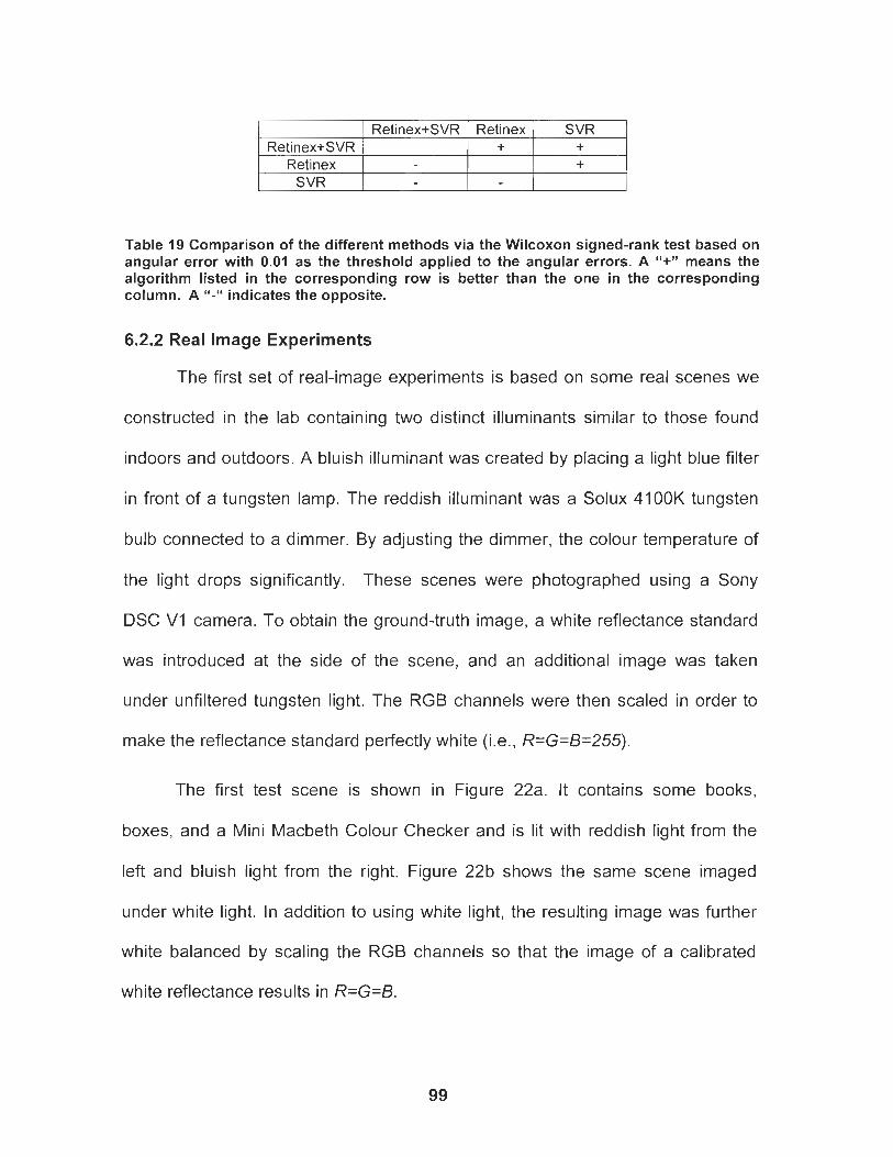
I Retinex+SVR I Retinex I SVR

Table 19 Comparison of the different methods via the Wilcoxon signed-rank test based on angular error with 0.01 as the threshold applied to the angular errors. A "+" means the algorithm listed in the corresponding row is better than the one in the corresponding column. A "-" indicates the opposite.

6.2.2 Real Image Experiments

The first set of real-image experiments is based on some real scenes we

constructed in the lab containing two distinct illuminants similar to those found

indoors and outdoors. A bluish illuminant was created by placing a light blue filter

in front of a tungsten lamp. The reddish illuminant was a Solux 4100K tungsten

bulb connected to a dimmer. By adjusting the dimmer, the colour temperature of

the light drops significantly. These scenes were photographed using a Sony

DSC V1 camera. To obtain the ground-truth image, a white reflectance standard

was introduced at the side of the scene, and an additional image was taken

under unfiltered tungsten light. The RGB channels were then scaled in order to

make the reflectance standard perfectly white (i.e., R=G=B=255).

Retinex

The first test scene is shown in Figure 22a. It contains some books,

boxes, and a Mini Macbeth Colour Checker and is lit with reddish light from the

left and bluish light from the right. Figure 22b shows the same scene imaged

under white light. In addition to using white light, the resulting image was further

white balanced by scaling the RGB channels so that the image of a calibrated

white reflectance results in R=G=B.

+ SVR

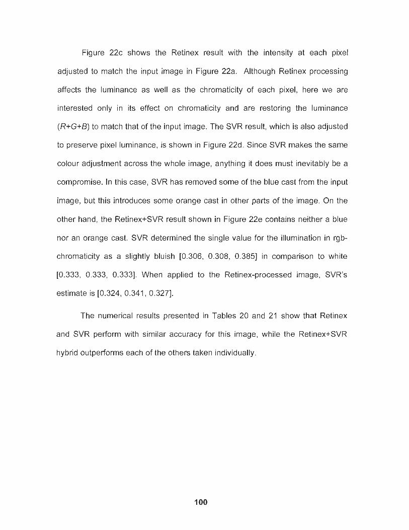
Figure 22c shows the Retinex result with the intensity at each pixel

adjusted to match the input image in Figure 22a. Although Retinex processing

affects the luminance as well as the chromaticity of each pixel, here we are

interested only in its effect on chromaticity and are restoring the luminance

(R+G+B) to match that of the input image. The SVR result, which is also adjusted

to preserve pixel luminance, is shown in Figure 22d. Since SVR makes the same

colour adjustment across the whole image, anything it does must inevitably be a

compromise. In this case, SVR has removed some of the blue cast from the input

image, but this introduces some orange cast in other parts of the image. On the

other hand, the Retinex+SVR result shown in Figure 22e contains neither a blue

nor an orange cast. SVR determined the single value for the illumination in rgb-

chromaticity as a slightly bluish [0.306, 0.308, 0.3851 in comparison to white

[0.333, 0.333, 0.3331. When applied to the Retinex-processed image, SVR's

estimate is [0.324, 0.341, 0.3271.

The numerical results presented in Tables 20 and 21 show that Retinex

and SVR perform with similar accuracy for this image, while the Retinex+SVR

hybrid outperforms each of the others taken individually.

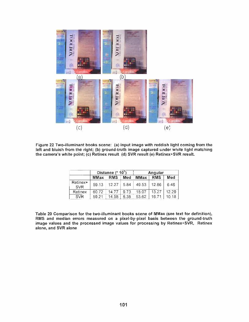
Figure 22 Two-illuminant books scene: (a) input image with reddish light coming from the left and bluish from the right; (b) ground-truth image captured under white light matching the camera's white point; (c) Retinex result (d) SVR result (e) Retinex+SVR result.

Table 20 Comparison for the two-illuminant books scene of MMax (see text for definition), RMS and median errors measured on a pixel-by-pixel basis between the ground-truth image values and the processed image values for processing by Retinex+SVR, Retinex alone, and SVR alone

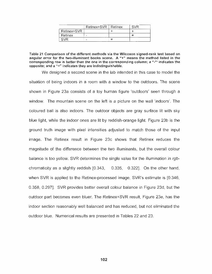
I Retinex+SVR I Retinex I SVR

Table 21 Comparison of the different methods via the Wilcoxon signed-rank test based on angular error for the two-illuminant books scene. A "+" means the method listed in the corresponding row is better than the one in the corresponding column; a "-"' indicates the opposite; and a "=" indicates they are indistinguishable.

Retinex+SVR 1

We designed a second scene in the lab intended in this case to model the

situation of being indoors in a room with a window to the outdoors. The scene

shown in Figure 23a consists of a toy human figure 'outdoors' seen through a

+

window. The mountain scene on the left is a picture on the wall 'indoors'. The

coloured ball is also indoors. The outdoor objects are gray surface lit with sky

blue light, while the indoor ones are lit by reddish-orange light. Figure 23b is the

ground truth image with pixel intensities adjusted to match those of the input

image. The Retinex result in Figure 23c shows that Retinex reduces the

+ Retinex

magnitude of the difference between the two illuminants, but the overall colour

balance is too yellow. SVR determines the single value for the illumination in rgb-

chromaticity as a slightly reddish 10.343, 0.335, 0.3221. On the other hand,

when SVR is applied to the Retinex-processed image, SVR1s estimate is [0.346,

0.358, 0.2971. SVR provides better overall colour balance in Figure 23d, but the

outdoor part becomes even bluer. The Retinex+SVR result, Figure 23e, has the

indoor section reasonably well balanced and has reduced, but not eliminated the

outdoor blue. Numerical results are presented in Tables 22 and 23.

- -

Figure 23 Window scene: (a) input image with bluish outdoor illumination and red-orange indoor illumination. (a) input image (b) ground-truth image captured under white light that matches the camera's white point; (c) Retinex result (d) SVR result (e) Retinex+SVR result

I Distance (* 10') I Angular I MMax 1 RMS I Med ( MMax I RMS I Med

Table 22 Comparison of MMax (see text for definition), RMS and median errors measured on a pixel-by-pixel basis between the ground-truth image values and the processed image values for processing by Retinex+SVR, Retinex alone, and SVR alone.

- - . . Retinex

SVR

Table 23 Comparison of the different methods via the Wilcoxon signed-rank test based on angular error for the window scene. A "+" means the method listed in the corresponding row is better than the one in the corresponding column. A "-"' indicates the opposite.

50.05 40.17

In addition to laboratory scenes, we processed images of other typical

Retinex+SVR Retinex SVR

scenes. The advantage of the laboratory scenes is that it is possible to obtain a

11.98 9.76

Retinex +

+

Retinex+SVR

ground truth image with which to evaluate the error in illumination estimation.

SVR + -

Outside the laboratory, it is difficult to make enough measurements of the

4.85 6.26

56.33 43.26

13.38 10.94

8.39 7.83

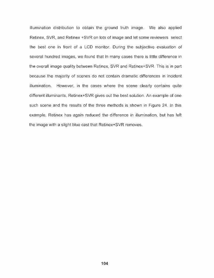
illumination distribution to obtain the ground truth image. We also applied

Retinex, SVR, and Retinex +SVR on lots of image and let some reviewers select

the best one in front of a LCD monitor. During the subjective evaluation of

several hundred images, we found that in many cases there is little difference in

the overall image quality between Retinex, SVR and Retinex+SVR. This is in part

because the majority of scenes do not contain dramatic differences in incident

illumination. However, in the cases where the scene clearly contains quite

different illuminants, Retinex+SVR gives out the best solution. An example of one

such scene and the results of the three methods is shown in Figure 24. In this

example, Retinex has again reduced the difference in illumination, but has left

the image with a slight blue cast that Retinex+SVR removes.

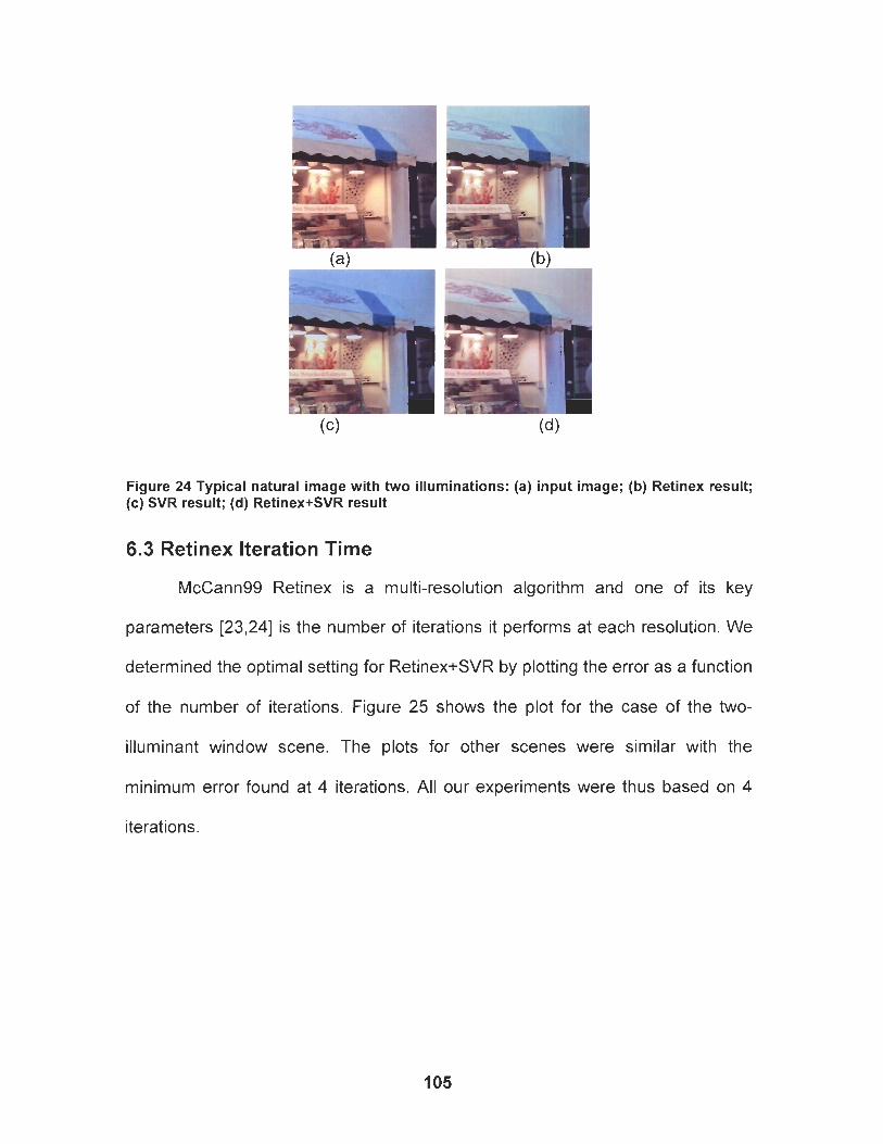
Figure 24 Typical natural image with two illuminations: (a) input image; (b) Retinex result; (c) SVR result; (d) Retinex+SVR result

6.3 Retinex Iteration Time

McCann99 Retinex is a multi-resolution algorithm and one of its key

parameters 123,241 is the number of iterations it performs at each resolution. We

determined the optimal setting for Retinex+SVR by plotting the error as a function

of the number of iterations. Figure 25 shows the plot for the case of the two-

illuminant window scene. The plots for other scenes were similar with the

minimum error found at 4 iterations. All our experiments were thus based on 4

iterations.

c .- ; lo. P

8 -

6 1 2 3 4 5 6 7 8 9 1 0

Number of Iterations

Figure 25 Median angular error as a function of the number of iterations Retinex used at each resolution. This plot is for the two-illuminant window scene; however, for other scenes the results are qualitatively similar.

6.4 Discussion

Many images are of scenes with at least two distinct illuminants. These

images present a challenge for automatic white balancing algorithms because

there is no single right answer. Retinex is one method that makes local

adjustments for the illumination, but it does not always get the overall colour

balance correct. We proposed a hybrid Retinex+SVR method and shown, at least

for the limited set of images it is possible to create in the laboratory, that it works

better than either SVR or Retinex working separately.

SVR is not the only illumination-estimation method that could be

hybridized with Retinex. Since there are several learning-based illumination

methods [I-5,32-361 of similar accuracy, it is reasonable to suppose that any one

of them could be substituted for SVR in this context with similar results.

Our goal was to remove the colour effects of illumination; however, as

Hubel [79] has argued perhaps in terms of creating an interesting image it is best

to preserve the illumination effects.

CHAPTER 7: INDEPENDENT COMPONENT ANALYSIS AND NONNEGATIVE LINEAR MODEL ANALYSIS OF

ILLUMINANT AND REFLECTANCE SPECTRA'

The colour outputs can be viewed as the projection of colour spectra on

the imaging device sensitivity functions. Another accurate way to represent any

location's colour is to provide the spectrum value at each wavelength. To reduce

storage and processing requirements, Principal Component Analysis (PCA),

lndependent Component Analysis (ICA), Non-Negative Matrix Factorization

(NNMF) and Non-Negative lndependent Component Analysis (NNICA) are all

techniques that can be used to compute basis vectors for finite-dimensional

models of spectra. The two non-negative techniques turn out to be especially

interesting because the pseudo-inverse of their basis vectors is also close to

being non-negative. This means that after truncating any negative components of

the pseudo-inverse vectors to zero, the resulting vectors become physically

realizable sensors functions whose outputs map directly to the appropriate finite-

dimensional weighting coefficients in terms of the associated (NNMF or NNICA)

basis. Experiments show that truncating the negative values incurs only a very

slight performance penalty in terms of the accuracy with which the input

spectrum can be approximated using a finite-dimensional model.

1 This chapter also appears as a published paper: Weihua Xiong and Brian Funt, "lndependent Component Analysis and Nonnegative Linear Model Analysis of llluminant and Reflectance Spectra", Proc. 10th Congress of the International Colour Association, Granada, May 2005

l o 8

7. 1 Introduction

Finite-dimensional models of spectra based on PCA have been widely

used since Judd's model of daylight and Cohen's analysis of Munsell chips.

Previous studies have applied ICA to surface reflectance [80] and daylight

spectra 1811. In this chapter, we extend this analysis to a larger set of illuminants

and to colour signal spectra. The colour signal is defined as the product of

surface reflectance and spectral power distribution of the illuminant incident on it.

We compare the PCA and ICA bases to the entirely non-negative bases obtained

via NNlCA and NNMF in terms of the accuracy with which full spectra can be

modelled using the various bases.

For any finite-dimensional model, a spectrum is modelled by projecting it

onto the pseudo-inverse of a set of basis vectors. This projection yields the

weighting coefficients of the model as described in more detail below. The output

of an optical sensor can also be described as the result of a projection of the

incoming spectrum on the sensor's spectral sensitivity functions. This leads to

the question: Is there a good basis for modelling spectra that also has the

property that the pseudo-inverse of the basis might be used as physically

realizable sensors?

PCA is a standard technique for calculating a good orthogonal basis from

a training set of spectra. However, being orthogonal, the PCA basis vectors

contain significant negative components. The pseudo-inverse of this basis is also

orthogonal and similarly contains significant negative components. As a result,

the PCA basis is unlikely to yield physically realizable sensors since such sensor

clearly can not have negative sensitivity; however, we hypothesize that perhaps

NNlCA and NNMF which yield non-negative basis vectors might. Such a sensor

would directly output the weighting coefficients of a finite-dimensional model of

the incident light's spectrum.

7.2 Method

It is convenient to express a finite-dimensional linear model of spectra as:

X = AB where X is an m-by-d matrix of m spectra each uniformly sampled at d

wavelengths; B is an n-by-d matrix of n basis vectors; and A is the m-by-n

mixing matrix of weighting coefficients. Since the intent of the dimensionality

reduction techniques is to identify a basis of reduced dimension that

approximates the original data well, n is generally less than m. Each of the four

dimensionality reduction techniques finds a basis B minimizing (possibly subject

to additional constraints):

PCA finds basis vectors that are uncorrelated and orthogonal. ICA finds

basis vectors that are uncorrelated and in addition are independent but not

orthogonal. There are many different ICA algorithms [82]. Here we used the

JADE [83] (Joint Approximate Diagonalization of Eigenvalues) implementation.

NNlCA [84] carries out ICA subject to the additional constraint of non-negativity

in the resulting basis vectors. Non-negative Matrix Factorization solves (37)

subject to all entries in both A and B being nonnegative. An iterative algorithm

1851 to do this is based on the following pair of equations:

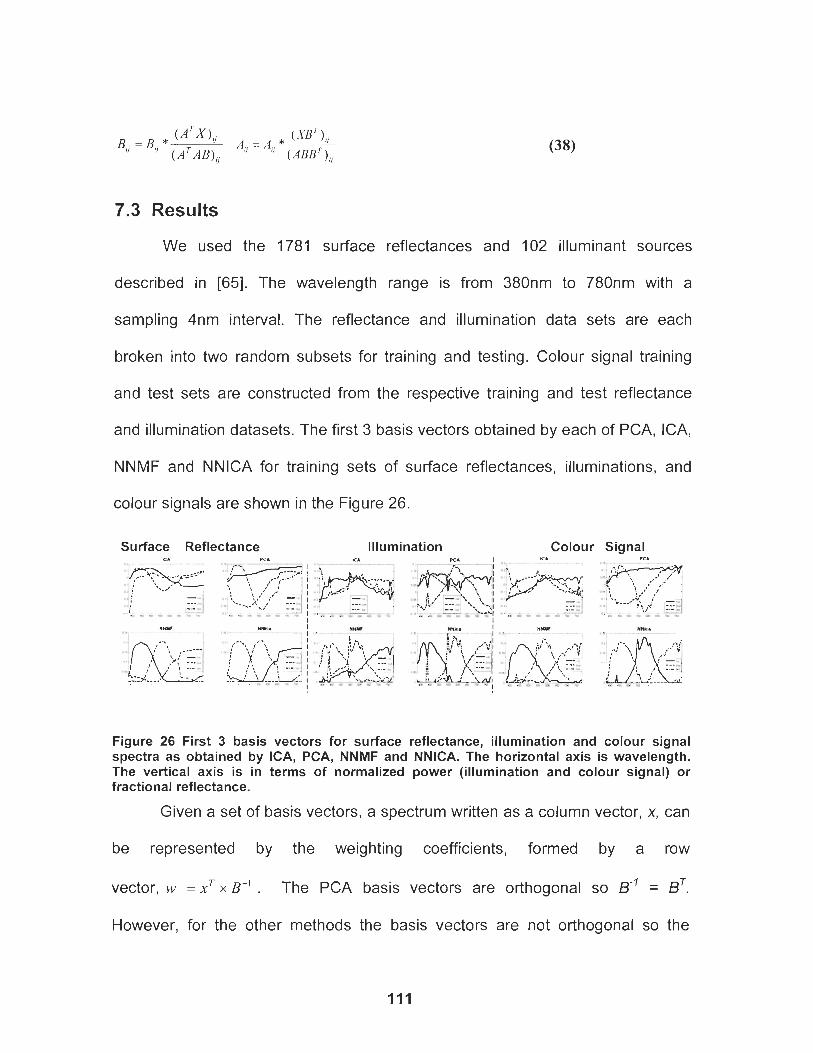
7.3 Results

We used the 1781 surface reflectances and 102 illuminant sources

described in [65]. The wavelength range is from 380nm to 780nm with a

sampling 4nm interval. The reflectance and illumination data sets are each

broken into two random subsets for training and testing. Colour signal training

and test sets are constructed from the respective training and test reflectance

and illumination datasets. The first 3 basis vectors obtained by each of PCA, ICA,

NNMF and NNICA for training sets of surface reflectances, illuminations, and

colour signals are shown in the Figure 26.

Figure 26 First 3 basis spectra as obtained by The vertical axis is in fractional reflectance.

t vectors for surface reflectance, illumination and colour signal ICA, PCA, NNMF and NNICA. The horizontal axis is wavelength. terms of normalized power (illumination and colour signal) or

Given a set of basis vectors, a spectrum written as a column vector, x, can

be represented by the weighting coefficients, formed by a row

vector, w = sT x B-' . The PCA basis vectors are orthogonal so B-' = BT.

However, for the other methods the basis vectors are not orthogonal so the

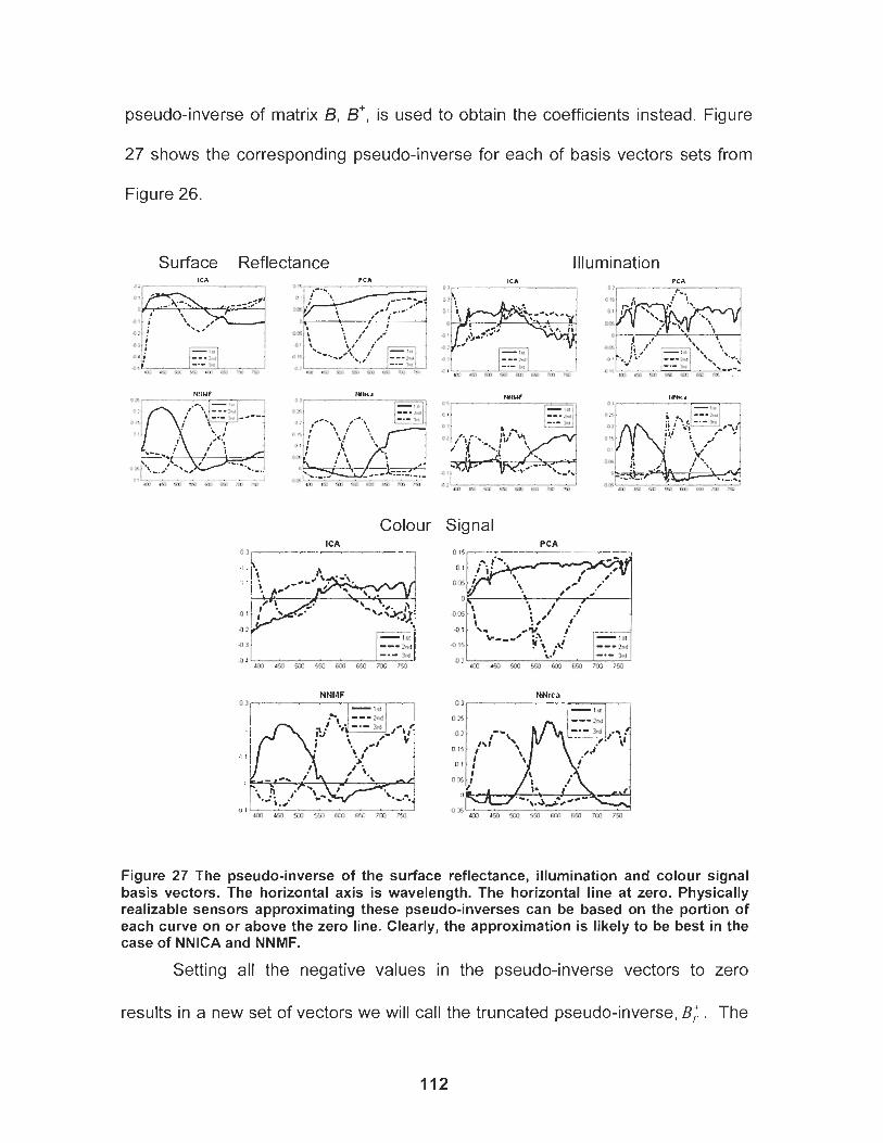
pseudo-inverse of matrix B, B', is used to obtain the coefficients instead. Figure

27 shows the corresponding pseudo-inverse for each of basis vectors sets from

Figure 26.

Surface Reflectance ICA PC4

Illumination

Colour ICA

I

Signal PC A

Figure 27 The pseudo-inverse of the surface reflectance, illumination and colour signal basis vectors. The horizontal axis is wavelength. The horizontal line at zero. Physically realizable sensors approximating these pseudo-inverses can be based on the portion of each curve on or above the zero line. Clearly, the approximation is likely to be best in the case of NNlCA and NNMF.

Setting all the negative values in the pseudo-inverse vectors to zero

results in a new set of vectors we will call the truncated pseudo-inverse, B,' . The

weighting coefficients are then obtained as w = x x B,' . An approximation, xl, , to

the original spectrum is reconstructed from the weights and basis as x,, = w x B .

The root mean square distance is one the measure of the accuracy of the

approximation of xu to .v :

We found that the L1 norm yielded qualitatively similar results to the RMS

error and therefore report only the RMS error. For N spectra the mean RMS error

is then simply the mean of the individual RMS errors:

When the true pseudo-inverse of basis vectors is used, ICA always results

in the least error. Figure 28 shows the mean approximation error as a function of

the number of basis vectors used. Plots of the median RMS error are qualitatively

similar.

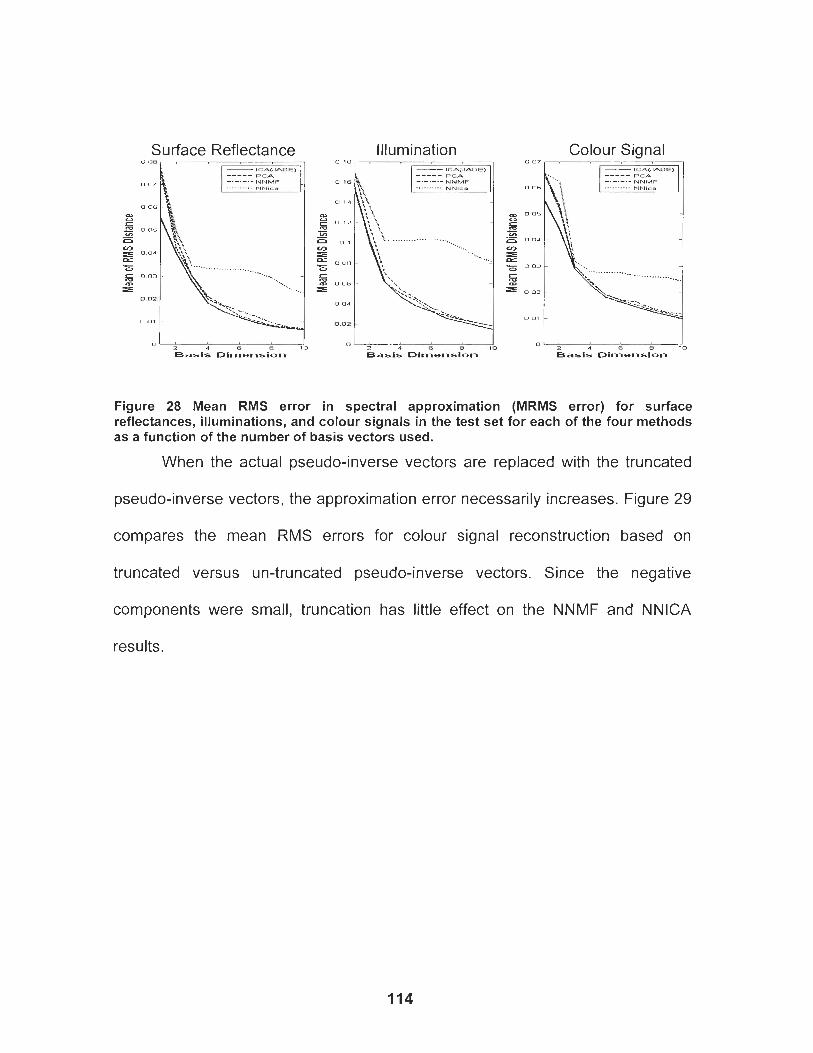
Surface Reflectance Illumination Colour Sianal

I . 2 4 e Basls Dlmiiension Bask DI~nensIon Basis Dlnienslo~i

Figure 28 Mean RMS error in spectral approximation (MRMS error) for surface reflectances, illuminations, and colour signals in the test set for each of the four methods as a function of the number of basis vectors used.

When the actual pseudo-inverse vectors are replaced with the truncated

pseudo-inverse vectors, the approximation error necessarily increases. Figure 29

compares the mean RMS errors for colour signal reconstruction based on

truncated versus un-truncated pseudo-inverse vectors. Since the negative

components were small, truncation has little effect on the NNMF and NNlCA

results.

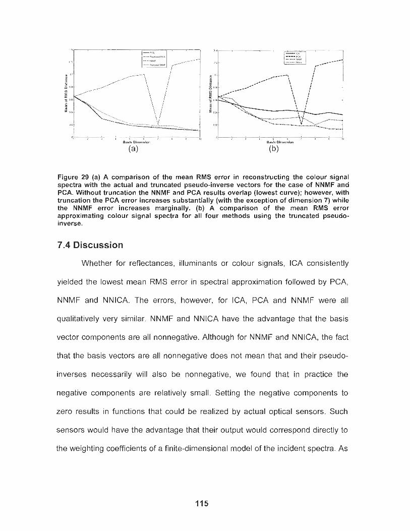
Figure 29 (a) A comparison of the mean RMS error in reconstructing the colour signal spectra with the actual and truncated pseudo-inverse vectors for the case of NNMF and PCA. Without truncation the NNMF and PCA results overlap (lowest curve); however, with truncation the PCA error increases substantially (with the exception of dimension 7) while the NNMF error increases marginally. (b) A comparison of the mean RMS error approximating colour signal spectra for all four methods using the truncated pseudo- inverse.

7.4 Discussion

Whether for reflectances, illurninants or colour signals, ICA consistently

yielded the lowest mean RMS error in spectral approximation followed by PCA,

NNMF and NNICA. The errors, however, for ICA, PCA and NNMF were all

qualitatively very similar. NNMF and NNICA have the advantage that the basis

vector components are all nonnegative. Although for NNMF and NNICA, the fact

that the basis vectors are all nonnegative does not mean that and their pseudo-

inverses necessarily will also be nonnegative, we found that in practice the

negative components are relatively small. Setting the negative components to

zero results in functions that could be realized by actual optical sensors. Such

sensors would have the advantage that their output would correspond directly to

the weighting coefficients of a finite-dimensional model of the incident spectra. As

such, they could be considered optimal (ignoring the influence of noise) in terms

of the information they capture about the incident spectra.

CHAPTER 8: CONCLUSION

With the development of multimedia and virtual reality technology, colour

information is being utilized widely and comprehensively in computer vision and

pattern recognition applications, such as image segmentation and object

recognition. But colour is one of the most complex phenomena of visual

perception. Colour perception is derived from the interactions between the visual

system, physical surfaces, illumination, and the visual environment. It is strongly

dependent on lighting geometry (direction and intensity of light sources) and

illuminant colour (spectral power distribution), which changes with the position

and atmospheric conditions. A fundamental and challenging issue is to separate

the illumination information from the image and recover the original surface

colour. This desired invariance of colour representation to general changes in

illumination is called colour constancy.

My dissertation has described my research work including new models of

colour constancy. The first contribution is to propose two new statistical

illumination colour estimation methods, one is based on the regression technique

and the other one is based on the interpolation technique. It is well known that

there is some relationship between the colour distribution of an image and its

illumination, and some research has been conducted to investigate this

phenomenon, for example, Colour by Correlation by Finlayson et. al., and Neural

Network by Funt et. al.. However, Neural Network may suffer from local

optimization. To overcome this disadvantage, I implemented Support Vector

Regression, a simple and better global solution, for predicting illumination

chromaticity values. The other solution is to extend a typical non-uniform

interpolation technique, Thin Plate Spline, into higher dimensions and extract a

continuous function representing the relationship between image colours and the

corresponding scene illumination. Compared with SVR, TPS has a major

advantage in that its outputs are always parameter-independent and unique.

The second contribution in my thesis is to design a fast and efficient colour

constancy method by designing a new colour coordinate system, named LIS.

This system can separate the illumination, intensity and surface information from

colour images as independently as possible. The surface axis is used to identify

those gray surfaces in the scene. Obviously the average of all RGB values of

these gray surfaces can be used to estimate the illumination chromaticities.

The third important contribution is to recover the original surface image by

integrating a spatially dependent method with a colour constancy solution for

those scenes under two or more sources of illumination. Until now, almost all

colour constancy algorithms assume either that there is only one uniform

illumination or that the illumination change is very smooth. These cases are not

true for most scenes. My work supposes that the surface orientation may cause

an illumination discontinuity. So the basic idea is to find those surfaces on the

same plane by stereo image technique, and apply a spatially dependent method

on the different planes separately. To avoid the problem that the Retinex method

tends to push isolated patches to gray, LIS is applied again here. The results

indicate the spatial arrangement can improve the colour constancy calculation.

However, this method requires one or more images captured of the same scene

simultaneously to detect the objects' depth information and surface orientation.

Such a limitation makes the method less practical, so the question of how to

solve this problem is a potential research direction in the next stage.

The fourth contribution is to design a hybrid colour constancy solution for

any single image under multiple sources of illumination. Retinex can be used to

mitigate the illuminations' difference and to create an intermediate image

assumed to be lit by an unknown consistent light, then the SVR global

illumination method and Von Kris diagonal transformation is applied to remove

the illumination effect. Although this method has been tested on several sets of

images, including synthetic images and real images, the performance of natural

images is not effective enough for practical uses. Thus improvement on it is

another possible research work in the future.

The fifth contribution is presented by research on the finite dimensional

model of colour spectra. PCA and ICA are commonly used to reduce the storage

and processing requirements for illumination and surface reflectance spectra. I

introduced two non-negative component analysis tools: NNMF and NNica. They

are shown not only to be accurate but also to be an efficient way to find the

optimal sensor sensitivity for the imaging device in terms of spectral estimation or

recovery.

REFERENCES

[ I ] B-Buchsbaum. "A spatial processor model for object color perception", Journal

of the Franklin Institute, 1980, Vol. 31, ppl -26

[2] G.D. Finlayson, and E. Trezzi, "Shades of Gray and Colour Constancy",

Proceedings of lz th Color Imaging Conference, 2004, pp. 37-41

[3] B. Funt and V.C. Cardei, "Bootstrapping colour constancy", Proc. Of SPIE,

Vol. 3644 1999, pp. 421 -428

[4] V. Cardei, B. Funt, and K. Barnard, "Estimating the Scene Illumination

Chromaticity Using a Neural Network", Journal of the Optical Society of America

A, Vol. 19, No. 12, Dec 2002, pp2374-2386.

[5] G. D. Finlayson, S. Hordley, and P. M. Hubel, "Color by Correction: A Simple,

Unifying Framework for Color Constancy", IEEE Transactions On Pattern

Analysis And Machine Intelligence Vo1.23, No. 1 1 Nov. 2001, pp.1209-1221

[6] T.K. Sarkar, "History of Wireless", Wiley-Interscience, 2006, pp20-66

[7] Mark D. Fairchild "Color Appearance Models", Wiley & Sons. Ltd 2005 pp.

146-1 50

[8] G. Wyszecki & W.S. Stiles, "Color Science: Concepts and Methods,

Quantitative Data and Formulas", 2nd edition, John Wiley & Sons, New York,

1 982, ~ ~ 7 4 - 1 0 3

[9] V. Kries. "Influence of adaptation on the effects produced by luminous stimuli"

Sources of Color Science, The MIT Press, Cambridge MA, 1970, pp. 109-1 19

[ l o ] M.R. Luo and R. W. G. Hunt. "A chromatic adaptation transform and a colour

inconstancy index". Color Res. Appl., Vol. 23, 1 998, pp. 1 54-1 58.

[ I I ] K. M. Lam. "Metamersim and Colour Constancy". PhD thesis, University of

Bradford, 1985.

[I21 D.H. Foster, S. M. C. Nascimento, "Four issues concerning colour constancy

and relational colour constancy1'. Vision Research, Vol. 37, lssue 10,

1997,pp.341-350.

1131 J.L. Simonds, "Application of characteristic vector analysis to photographic

and optical response data", Journal of the Optical Society of America A, Vol. 53,

Issue. 8, 196, pp. 968-974

[I41 K. Barnard, L. Martin, A. Coath, and B. Funt, "A Comparison of

Computational Colour Constancy Algorithms. Part Two: Experiments on lmage

Data", IEEE Transactions on lmage Processing, No. 11, 2002, pp.985-996 .

[I51 K. Barnard, V. Cardei, and B. Funt, "A Comparison of Computational Colour

Constancy Algorithms. Part One: Methodology and Experiments with

Synthesized Data", IEEE Transactions on lmage Processing, No. 1 1,2002, pp.

972-984 .

[I61 L.T. Maloney and B.A. Wandell, "Color Constancy: A Method for Recovering

Surface Spectral Reflectance", Journal of the Optical Society of America A, Vol.

3, lssue 1, 1986, pp.29-33

[I71 B.A. Wandell, "The synthetic and Analysis of Color Images", IEEE

Transactions on PAMI, No. 1, lssue 9, January, I987 ppl-13

1181 J.Cohen, "Dependency of the spectral reflectance curves of the Munsell

colour chips", Psychonomic Science, Vol. 1, 1964, pp369-370

[ I 91 L.T. Malony, "Evaluation of linear models of surface spectral reflectance with

small numbers of parameters," Journal of the Optical society of America A, Vol.

3, 1986, ~~1673 -1683

[20] J.P.S. Parkkinen, J.Hallikainen, and T. Jaaskelainen, "Characteristic spectra

of Munsell colors", Journal of the Optical society of America A, Vol. 6, 1989,

~ ~ 7 2 5 - 7 3 0

[21] H.Laamanen, T. Jaaskelainen, J.P.S. Parkkinen, and J.Hallikainen,

"Comparison of PCA and ICA in color recognition", Proceedings of SPIE, Vol.

41 97,2000

[22] E. Land, J. McCann, "Lightness and Retinex Theory", Journal of the Optical

Society of America A, Vol. 61, January 1971, pp. 1-1 1

[23] B. Funt, F. Ciurea, J. McCann, "Retinex in Matlab", Journal of the Electronic

Imaging, Jan. 2004, pp 48-57

[24] B. Funt, and F. Ciurea, "Parameters for Retinex", Proc. 9th Congress of the

International Color Association, Rochester, June 200 1 .

[25] B. Funt, F. Ciurea, and J. McCann, "Tuning Retinex Parameters", Journal of

the Electronic Imaging, Jan. 2004, pp 48-57.

[26] Jr. T.G. Stockham, "Image processing in the context of a visual model1',

Proc. of IEEE. Vol. 60, Issue 1072,pp. 828-842

1271 O.D. Faugeras, "Digital image color processing within the framework of a

human visual system1', IEEE transactions on ASSP, Vol. 27, 1979, pp380-393

[28] B.K.P. Horn, "Determining lightness from an image", Computer Graphics and

lmage Processing, Vol. 3, 1974, pp277-299

[29] J. Frankle, Jonathan and J. McCann, "Method and Apparatus for Lightness

Imaging", US Patent #4,384,336, May 17, I983

[30] R. Kimmel, M. Elad, D. Shaked, R. Keshet, and I. Sobel, "A Variational

Framework for Retinex", International Journal of Computer Vision, Vol. 52, Issue

1, 2003, pp7-23

[31] G. D. Finlayson and S. Hordley, "Selection for Gamut Mapping Color

Constancy", British Machine Vision Conference, 630-639, Sept. 1997.

[32] G.D. Finlayson. "Retinex viewed as a gamut mapping theory of color

constancy", Proc. AIC lnternational Association 97, Vol. 2, 1997, pp. 527-530

[33] S.D. Hordley, "Scene Illumination Estimation: Past, Present, and Future",

Color Research and Application, Vol. 31, Number 4, 2006, pp. 303-31 4

[34] J. Weijer, and Th. Gevers, "Color Constancy based on the Grey-Edge

Hypothesis", Proceedings of I International Conference on lmage

Processing, 2005, pp. 722-725

[35] K. Barnard, L. Martin, and B. Funt, "Colour by correlation in a three

dimensional colour space'', 6th European Conference on Computer Vision, 2000,

~ ~ 3 7 5 - 3 8 9

[36] C. Rosenberg, M. Hebert and S. Thrun, "Color constancy using KL-

divergence", Proc. 8'h ICCV, Vol. 1, 2001, pp. 239-246

[37] A.L. Gilchrist, "Perceived lightness depends on perceived spatial

arrangement," Science, Vol. 195, 1977, pp. 185-1 87

[38] Y. Yamauchi, K. Uchikawa, "Depth Information Affects Judgment of the

Surface-Color Mode Appearance", Journal of Vision, Vol. 5, 2005, pp.515-523

[39] J. N. Yang, S.K. Shevell, "Stereo Disparity Improves Color Constancy,"

Vision Research, Vol. 42, 2002, pp. 1979-1989

[40] H. Boyaci, L.T. Maloney, S. Hersh, "The Effect of Perceived Surface

Orientation on Perceived Surface Albedo in Binocularly Viewed Scenes", Journal

of Vision, Vol. 3, 2003, pp. 541-553

[41] J.N. Yang, L.T. Maloney, "llluminant cues in surface color perception: Tests

of three candidate cues", Vision Research, Vol. 41, 2001, pp. 2581-2600

[42] L.T. Maloney, M. S. "illumination Estimation as Cue Combination", Journal of

Vision, Vo1.2, 2002, pp493-504.

[43] G. Finlayson, M. Drew, and B. Funt, "Color constancy: generalized diagonal

transforms suffice", Journal of the Optical Society of America, A No. 11, 1994,

pp.3011-3020.

[44] B. Funt, V. Cardei and K. Barnard, "Learning Color Constancy", Proc.

IS&T/SID Fourth Color Imaging Conference: Color Science, Systems and

Applications, 1996, pp. 58-60

[45] A. Smola and B. Scholkopf, "A tutorial on support vector regression",

Statistics and Computing, 2003

[46] V. Kecman, Learning and Soft Computing, MIT, Cambridge, 2001, pp. 121-

193

[47]A. Chodorowski, T. Gustavsson and U. Mattson, "Support Vector Machine for

Oral Lesion Classification", Proceedings of 2002 IEEE International Symposium

on Biomedical Imaging, July, 2002, pp.173 - 176

[48] C.W. Hsu and C.J. Lin, "A Comparison of Methods for Multiclass Support

Vector Machine", IEEE Transaction on Neural Network, 2002, Vol. 13 No 2,

pp.415-425

[49] Y. Lee and C. Lee, "Classification of Multiple Cancer Types by Multicategory

Support Vector Machines using Gene Expression Data Bioinformatics",

Bioinformatics Vol. 19 No. 9, 2003 pp. 11 32-1 139

[50] Y.Lee, Y.Lin and G. Wahba, "Multicategory Support Vector Machine",

Proceedings of the 33rd Symposium on the Interface, 2001

[51] H. Yang, L. Chan, and I. King, "Support Vector Machine Regression for

Volatile Stock Market Prediction", lntelligent Data Engineering and Automated

Learning 2002, LNCS 24412, 2002, pp. 391-396

[52] C.H. Wu, C. C. Wei, M.H. Chang, D.C. Su and J.M. Ho, "Travel Time

Prediction with Support Vector Regression", Proc. Of IEEE lntelligent

Transportation Conference, October, 2003, pp. 1438-1442.

[53] D. X. Zhao, and L. Jiao, "Traffic Flow Time Series Prediction Based On

Statistics Learning Theory", Proceedings of IEEE 5th International Conference on

lntelligent Transportation Systems, 2002, pp. 727-730

1541 H. V. Khuu, H.K. Lee and J.L. Tsai, "Machine Learning with Neural Networks

and Support Vector Machines", Online Technical Report, available at:

http://www.cs.wisc.edu/-hiep/Sources/Articles/, accessed on April, 2004

[55] C.C. Chang, and C.J. Lin(2001), LIBSVM: a library for support vector

machines. Software available at http://www.csie, ntu.edu. tw/-cilin/libsvm,

accessed on April, 2004

1561 NJ. Bi and K. P. Bennett, "A Geometric Approach to Support Vector

Regression, Neurocomputing7', Vol. 55, Issues 1-2, 2003, pp. 79-108

[57] K. Barnard, L. Martin, and B. Funt, "Colour by correlation in a three

dimensional colour space", 6th European Conference on Computer Vision,

Springer, 2000, pp. 375-389.

[58] G.D. Knott, Interpolating Cubic Splines, Birkhauser Inc, 2000

1591 F. L. Bookstein. "Principal warps: thin-plate splines and decomposition of

deformations", IEEE Trans. Pattern Analysis and Machine Intelligence, Vol. 11,

lssue 6, 1989, pp. 567-585.

[60] M. H. Davis, A. Khotanzad, D. Flamig, and S. Harms. "A physics-based

coordinate transformation for 3-d image matching", IEEE Trans. Medical Imaging,

Vol. 16, lssue 3, 1997, pp.317-328.

[61] N. Arad and D. Reisfeld, "Image warping using few anchor points and radial

functions", Computer Graphics forum, pp.35-46, vol. 14, 1995, pp. 35-46.

[62] Asker M. Bazen and Sabih H. Gerez, "Elastic minutiae matching by means

of thin-plate spline models", International Conference on Pattern Recognition,

Aug 2002

[63] W. Xiong and B. Funt, "Nonlinear RGB-to-XYZ Mapping for Device

Calibration", Proceedings of the 13'~ CIC, 2005, pp. 200-204

[64] G.D. Finlayson and S.D. Hordley, "Color Constancy at a pixel", Journal of the

Optical Society of America A, Vol. 18, issue 2, 2001, pp. 253-64

[65] K. Barnard, L. Martin, B. Funt, A. Coath, "A Data Set for Color Research",

Colour Research and Application, Vol. 27 No. 3, 2002, pp. 140-147. (Data from:

www.cs.sfu .cat-colour )

[66] http://www,mathworks.com/, accessed on January 2006

[67]S.D. Hordley, G.D. Finlayson, "Reevaluation of color constancy algorithm

performance", Journal of the Optical Society of America A, vol. 23, Issue 5, 2006,

pp. 1008-1 020

[68] K. Barnard, and B. Funt, "Camera Characterization for Color Research",

Colour Research andApplication, Vol. 27, No. 3, 2002, pp. 153-164.

[69] www.cs.sfu.ca/-colour, accessed on January 2006

[70] F. Ciurea and B. Funt, "A Large Image Database for Color Constancy

Research", Proc. IS&T.SID Eleventh Color lmaging Conference, Society for

lmaging Science and Technology, 2003, pp. 160-1 63.

[71] R.L. Eubank, Spline Smoothing and Nonparametric Regression, Marcel

Dekker, New York, 1988

[72] M.G. Bloj., D. Kersten, A.C. Hurlbert, "Perception of Three-Dimensional

Shape Influences Colour Perception through mutual Illumination", Nature, Vol.

42, 1999, pp. 23-30

[73] E.H. Adelson. "Lightness Perception and Lightness Illusions," New Cognitive

Neuroscience, 2"d ed., MIT Press, 2000, pp. 339-351

[74] M. Gelautz, D. Markovic, "Recognition of Object Contours from Stereo

Images: an Edge Combination Approach", Proc. Of Yd International Symposium

on 3 0 Data Processing, Visualization and Transmission, 2004, pp. 774-780

[75] Ch. Sun, "Fast Stereo Matching Using Rectangular Subregioning and 3D

Maximum-Surface Techniques", International Journal of Computer Vision. Vol.

47,2002, pp. 99-1 17

[76] http://ww.loreo.com , accessed on September 2005

[77]http://www.vision.caltech .edu/bouqueti/calib doc/, accessed on September

2005

[78] www.qretaqmacbeth.com, accessed on September 2005

[79] P. M. Hubel, "The Perception of Colour at Dawn and Dusk", Proc. fh Color

lmaging Conference, 1999, pp.48-51

[80] H. Laamanen, T. Jaaskelainen, and J.P.S. Parkkinen, "Comparison of PCA

and ICA in color recognition", Proceedings of Intelligent Robots and Computer

Vision, SPlE vol. 4197, 2000, pp. 367-377

[81] Eva M. Valero, Juan L. Nieves, Javier Hernandez-Andres, and Javier

Romero, "lndependent component analysis with Different Daylight Illuminants",

Proc. Second European Conference on Colour in Graphics, Imaging and Vision,

2004,pp.I 93-1 96

[82] A. Hyvarinen, J. Karhunen and E. Oja, lndependent Component Analysis,

(John Wiley & Sons Inc, Part 11 2001) pp. 147-1 93.

[83] J. F. Cardoso and A.Souloumiac, "Blind Beamforming for Non Gaussian

Signals", IEEE Transactions on Signal Processing, Vol. 46, Issue 7, 1998, pp.

1878-1 885.

1841 M.D. Plumbley, "A Nonnegative PCA Algorithm for lndependent Component

Analysis", IEEE Transactions On Neural Network, Vol. 15, No 1, 2004, pp.66-76

[85] D.D. Lee and H.S. Seung, "Algorithms for Non-negative Matrix

Factorization", Advanced Neural Information Processing Systems, Vol. 13 , 43-56,

(2001 ).