SE—Structures and Environment: Acceptable Nitrate Concentration of Greenhouse Lettuce: Two Optimal Control Policies

Biosystems Engineering (2002) 83 (2), 199–215doi:10.1016/S1537-5110(02)00158-7, available online at http://www.idealibrary.com onSE}Structures and Environment

Acceptable Nitrate Concentration of Greenhouse Lettuce: Two Optimal ControlPolicies

Ilya Ioslovich; Ido Seginer

Agricultural Engineering Department, Technion, Haifa 32000, Israel; e-mail of corresponding author: [email protected]

(Received 11 January 2001; accepted in revised form 11 July 2002)

Greenhouse lettuce with high nitrate levels is unmarketable in the European Union. To avoid the loss of acrop, an economical environmental control strategy, based on a suitable crop model, is required. A recentlydeveloped dynamic lettuce growth model, in conjunction with a simple greenhouse model, is used here todevelop a strategy for hydroponic greenhouses where temperature and nitrate supply rate can be controlled.Two cases are considered: (1) fixed spacing, as in traditional systems and (2) potted or floating plants, wherecontinuously variable spacing can be used as a third control variable. The optimization criteria are formulatedfor a market-quota situation, and optimal control methodology is used to find the optimal strategies. Twosimplifying assumptions are made, (1) the weather is constant throughout the growing period and (2)photosynthesis and growth are not inhibited.

The results show that the optimal policy for the variable spacing systems is independent of the age ofthe crop. The canopy density (leaf area index) is maintained constant by continuously increasing the spacing,the optimal heating temperature alternates, and the optimal ventilation temperature is constant. If,under the prevailing light level, the minimum temperature cannot ensure a sufficiently low crop nitratecontent, the supply rate of nitrate must be reduced.

The optimal control policy for fixed spacing systems is to start with the highest permissible temperature andwith abundant nitrate supply. At certain points in time, a switch down to the temperature of unventilated andunheated greenhouse, and later to the lowest feasible temperature, may be required. Finally, a switch to thelowest permissible nitrate supply rate may also be needed.

Two variants of the variable-spacing system (fixed and free final state of the crop) are analysed first. Next,the fixed-spacing system (with fixed and free final state) is explored. An algorithmic solution method isoutlined for each of the cases and sample results are compared. # 2002 Silsoe Research Institute. Published by Elsevier

Science Ltd. All rights reserved

1. Introduction

High nitrate content in lettuce may be hazardous tohealth (MAFF, 1997), and it is well established thatcertain environmental conditions, in particular low lightlevel, are conducive to such an outcome. Recently, asimple dynamic lettuce growth model Nicolet (Segineret al., 1998, 1999) has been developed to predict nitratecontent, from the environmental history of the crop.The model is based on a source–sink balance for carbon,and on a turgor-maintenance relationship, which resultsin an often observed negative correlation betweencarbon and nitrate in the cell-sap (e.g. Drews et al.,1995). The availability of a crop model makes it possibleto develop an optimal control strategy for growing

1537-5110/02/$35.00 19

greenhouse lettuce; a strategy which maximises theprofits of the grower, subject to maintaining anacceptable level of nitrate content.

In this study, lettuce production systems are con-sidered where temperature and nutrient composition canbe controlled. Two rather different systems are treated:fixed plant spacing and continuously variable plantspacing. While the fixed-spacing system operates inbatch mode (conventional production), the variablespacing requires a continuous production system, whereplants of all ages are present in the greenhouse at thesame time (Both et al., 1999).

Plant spacing has a major effect on the totalproductivity of a crop, and variable spacing, as anelement of industrialised production of crops, has been

9 # 2002 Silsoe Research Institute. Published by

Elsevier Science Ltd. All rights reserved

I. IOSLOVICH; I. SEGINER200

Notation

a plant spacing, m2 [ground] plant–1

A;B mathematical terms [Eqn (60)], $mol–1 [C]bg border coefficient in the inhibition function hg

bp border coefficient in the inhibition function hp

c respiration exponent [Eqn (22)], K–1

CCa CO2 concentration in air, mol [C]m�3

e� specific respiration function, s–1

E time integral of the area in Table 1,m2 [ground] s plant�1

f � light interception function [Eqn (23)]FCij carbon flux from crop compartment

i to j, mol [C]m–2 [ground] s–1

FCg growth respiration carbon flux,mol [C]m�2 [ground] s�1

FCm maintenance respiration rate,mol [C]m–2 [ground] s–1

FCp photosynthesis carbon flux,mol [C]m�2 [ground] s�1

FL lower bound for FCvs [Eqn (32)],mol [C]m–2 [ground] s–1

FNu nitrate uptake flux,mol [N]m�2 [ground] s�1

FNvs nitrate flux from vacuole to structure,mol [N]m�2 [ground] s�1

FU upper bound for FCvs [Eqn (32)],mol [C]m–2 [ground] s–1

g� uninhibited growth rate of a closedcanopy, mol [C]m–2 [ground] s–1

G constant value determined in Eqn (11),Pam3mol–1 [C]

hg� growth inhibition function (hg ¼ 1 whenno inhibition)

hp� photosynthesis inhibition function(hp ¼ 1 when no inhibition)

H Hamiltonian, $mol–1 [C]I light intensity of photosynthetically

active photons (PAP),mol [PAP]m–2 [ground] s–1

J optimization criterion, $plant–1

k respiration coefficient [Eqn (22)], s–1

mCj carbon content of compartment j ofa single plant, mol [C] plant–1

MCj carbon content of crop compartment j,mol [C]m–2 [ground]

MNj nitrogen content of crop compartment j,mol [N]m–2 [ground]

N numerator [Eqn (43)], $m–2 [ground] s–1

N1 numerator [Eqn (52)], $m–2 [ground] s–1

p� uninhibited gross photosynthesis rate of aclosed canopy, mol [C]m–2 [ground] s–1

PH unit cost of heating, $m–2 [ground]K–1 s–1

Pm unit cost of structural carbon of the crop,$mol�1 [C]

PR unit cost of rent, $m–2 [ground] s–1

rN nitrogen to carbon ratio in structure,mol [N]mol�1 [C]

sg slope coefficient in the inhibition function hg

sp slope coefficient in the inhibition function hp

t time, sT greenhouse temperature, KTS temperature in an unheated and

unventilated greenhouse, KT� reference temperature [Eqn (22)], KV volume of water, m3m–2 [ground]a coefficient defined by Eqn (6), m3 mol�1 [C]bN coefficient [Eqn (9)], Pam3 mol–1 [N]bC coefficient [Eqn (9)], Pam3 mol–1 [C]g coefficient in Eqn (57)GCv normalised carbon concentration in vacuoleGNv normalised nitrate concentration in

vacuoled difference [Eqn (60)], $mol–1 [C]e light efficiency coefficient [Eqn (20)],

mol [CO2]mol�1 [PAP]y coefficient (growth respiration as fraction of

growth)l costate variable of carbon mass in the

vacuole mCv, $mol–1 [C]m gfTg=efTg, mol [C]m–2 [ground]s coefficient [Eqn (20)],

mol [air] m�2 [ground] m s�1

P osmotic pressure in vacuole, Pac exponent [Eqn (23)], m2 [ground]mol�1 [C]

Subscriptsa airC carbonf finalg growthi initialL lower boundm maintenanceN nitrogenn nutrient solutions crop structure compartmentU upper boundv crop vacuole compartment1–4 numbers of switching points of the

control along the trajectory (Fig. 4)

SuperscriptsD demandS supply

Other conventions{ } exclusively used to contain the arguments

of functions, the point in {�} being ashorthand notation for the arguments

FCp

Atmosphere (a)CCa

Maintenance respiration,

FCm

Growthrespiration,

FCg

Structure (s)MCs, MNsGrowth

FCvs, FNvs

Temperature

FNnv

Rhizospherenutrient solution (n)

Demand

MCv, MNv

Vacuoles (v)substrate poolTurgor control

Light, CO2

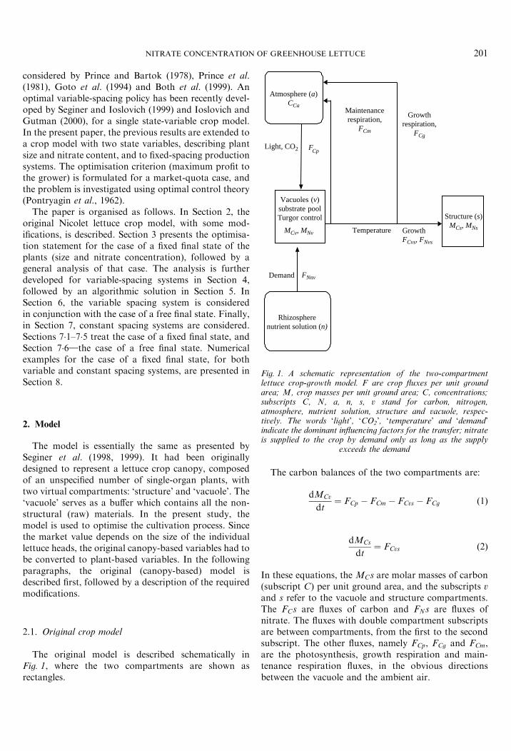
Fig. 1. A schematic representation of the two-compartmentlettuce crop-growth model. F are crop fluxes per unit groundarea; M, crop masses per unit ground area; C, concentrations;subscripts C, N, a, n, s, v stand for carbon, nitrogen,atmosphere, nutrient solution, structure and vacuole, respec-tively. The words ‘light’, ‘CO2’, ‘temperature’ and ‘demand’indicate the dominant influencing factors for the transfer; nitrateis supplied to the crop by demand only as long as the supply

exceeds the demand

NITRATE CONCENTRATION OF GREENHOUSE LETTUCE 201

considered by Prince and Bartok (1978), Prince et al.(1981), Goto et al. (1994) and Both et al. (1999). Anoptimal variable-spacing policy has been recently devel-oped by Seginer and Ioslovich (1999) and Ioslovich andGutman (2000), for a single state-variable crop model.In the present paper, the previous results are extended toa crop model with two state variables, describing plantsize and nitrate content, and to fixed-spacing productionsystems. The optimisation criterion (maximum profit tothe grower) is formulated for a market-quota case, andthe problem is investigated using optimal control theory(Pontryagin et al., 1962).

The paper is organised as follows. In Section 2, theoriginal Nicolet lettuce crop model, with some mod-ifications, is described. Section 3 presents the optimisa-tion statement for the case of a fixed final state of theplants (size and nitrate concentration), followed by ageneral analysis of that case. The analysis is furtherdeveloped for variable-spacing systems in Section 4,followed by an algorithmic solution in Section 5. InSection 6, the variable spacing system is consideredin conjunction with the case of a free final state. Finally,in Section 7, constant spacing systems are considered.Sections 7�1–7�5 treat the case of a fixed final state, andSection 7�6}the case of a free final state. Numericalexamples for the case of a fixed final state, for bothvariable and constant spacing systems, are presented inSection 8.

2. Model

The model is essentially the same as presented bySeginer et al. (1998, 1999). It had been originallydesigned to represent a lettuce crop canopy, composedof an unspecified number of single-organ plants, withtwo virtual compartments: ‘structure’ and ‘vacuole’. The‘vacuole’ serves as a buffer which contains all the non-structural (raw) materials. In the present study, themodel is used to optimise the cultivation process. Sincethe market value depends on the size of the individuallettuce heads, the original canopy-based variables had tobe converted to plant-based variables. In the followingparagraphs, the original (canopy-based) model isdescribed first, followed by a description of the requiredmodifications.

2.1. Original crop model

The original model is described schematically inFig. 1, where the two compartments are shown asrectangles.

The carbon balances of the two compartments are:

dMCv

dt¼ FCp � FCm � FCvs � FCg ð1Þ

dMCs

dt¼ FCvs ð2Þ

In these equations, the MCs are molar masses of carbon(subscript C) per unit ground area, and the subscripts v

and s refer to the vacuole and structure compartments.The FCs are fluxes of carbon and FNs are fluxes ofnitrate. The fluxes with double compartment subscriptsare between compartments, from the first to the secondsubscript. The other fluxes, namely FCp, FCg and FCm,are the photosynthesis, growth respiration and main-tenance respiration fluxes, in the obvious directionsbetween the vacuole and the ambient air.


The nitrogen balances are:

dMNv

dt¼ FNnv � FNvs ð3Þ

dMNs

dt¼ FNvs ð4Þ

where the subscripts N and n denote nitrogen anduptake from the nutrient solution, respectively. All thevacuolar nitrogen is considered to consist of nitrate,while all the structural nitrogen is considered to beorganic nitrogen (reduced-nitrogen).

Two constant compositional ratios are assumed:nitrogen-to-carbon in the structure, and water tostructural carbon

MNs ¼ rNMCs ð5Þ

V ¼ aMCs ð6Þ

where rN and a are the two proportionality coefficients.Constant proportions are also assumed among some ofthe fluxes. First, in view of Eqns (2) and (4), Eqn (5)implies

FNvs ¼ rNFCvs ð7Þ

Second, growth respiration is assumed to be aconstant fraction of growth, namely

FCg ¼ yFCvs ð8Þ

A central element of the model is the osmotic balance:

bCMCv þ bNMNv ¼ aPMCs ð9Þ

where: bC and bN are the osmotic pressures associatedwith one unit of vacuolar carbon or nitrogen and P isthe total osmotic pressure (assumed to be constant).This equation ensures that the combined osmoticcontribution of the vacuolar soluble carbon compoundsMCv and of the vacuolar nitrate MNv, together withother compounds that are well correlated with them, areconstant.

The model involves five constituents, namely MCs;MCv;MNs;MNv and V , constrained by three inter-relationships, Eqns (5), (6) and (9). Hence, the modelhas two state variables, chosen to be MCs and MCv.

Differentiating the osmotic balance, Eqn (9), withrespect to time, and substituting from Eqns (1)–(3), (7)and (8), results in the flux balance:

GFCvs � bNFNnv ¼ bCðFCp � FCmÞ ð10Þ

where

G ¼ aPþ bNrN þ bCð1 þ yÞ ð11Þ

is a collection of parameters. The two terms on the leftof Eqn (10) may be affected by the availability ofnitrogen in the nutrient solution, and have to beformulated differently for different nutritional situations

(abundant or limiting nitrogen). If one of them is given,the other can be determined from the equation, as willbe shown below.

The various fluxes need now to be expressed in termsof the state of the crop and its environment. For thispurpose, it is convenient to define normalised concen-trations, G, for the vacuolar material, namely

GCv bC

aPv

MCv

MCs

; GNv bN

aPv

MNv

MCs

ð12Þ

leading to a normalised-concentration osmotic balance,

GCv þ GNv ¼ 1 ð13Þ

The carbon fluxes of Eqn (10) are formulated as

FCp ¼ pfI ;CCagf fMCsghpfGCvg ð14Þ

FDCvs ¼ gfTgf fMCsghgfGCvg ð15Þ

FCm ¼ efTgMCs ð16Þ

Equation (15) describes the rate of structural growthwhen nutrients are abundant (superscript D indicatinggrowth according to crop demand). This may not be theactual growth rate, if nitrogen supply FS

Nnv (superscript S

for supply) is limited. All carbon fluxes are functions ofthe environment, namely: I , light; CCa, CO2 concentra-tion in the air and T , temperature; as well as of the stateof the crop, via MCs and GCv. The first factor in Eqns(14) and (15) is the potential flux, which only depends onthe environment. The factor f fMCsg, the effect of cropsize, approaches one as the crop grows. PhotosynthesisFCp may become inhibited, via hpfGCvg, when thevacuole approaches saturation with carbohydrates,and growth F D

Cvs may become inhibited, via hgfGCvg,when the vacuole is depleted of carbohydrates.

Equation (10) can be modified to test if the nutritionalsituation is of limited or unlimited nitrogen supply.Replacing the actual fluxes FCvs and FNv on the left ofEqn (10) by the demand and supply fluxes, the left-handside becomes either smaller or larger than the right-handside. If

GFDCvs � bNF S

Nv > bCðFCp � FCmÞ ð17Þ

then the instantaneous growth is nitrogen limited andgrowth must adjust to the limited nitrogen supply:

GFCvs ¼ bNFSNnv þ bCðFCp � FCmÞ ð18Þ

If the opposite is true, uptake must adjust to the lowgrowth potential

bNFNnv ¼ GF DCvs � bCðFCp � FCmÞ ð19Þ


Photosynthesis is formulated as a simplified Michaelis–Menten process. Respiration, and hence growth, areformulated as exponential functions of temperature:

Photosynthesis

pfI ;CCag ¼eIsCCa

eI þ sCCa

ð20Þ

Growth

gfTg ¼ mefTg ð21Þ

where

efTg ¼ k expfcðT � T�Þg ð22Þ

The coefficients e; s; k; c and m are constants and T� is anarbitrary reference temperature.

The dependence on crop size has the form

f fMCsg ¼ 1 � expf�cMCsg ð23Þ

and the inhibition functions hp and hg are given by

hpfGCvg ¼1

1 þ ðð1 � bpÞ=ð1 � GCvÞÞsp

ð24Þ

hgfGCvg ¼1

1 þ ðbg=GCvÞsg

ð25Þ

where c, bp, bg, sp and sg are constant coefficients.

2.2. Modifications to crop model

The state variables of the new model representindividual plants. They are derived from the originalcanopy variables by multiplying with the area occupiedby a single plant. Since this area may vary with time, it isrepresented by aftg. Hence,

mCv ¼ aftgMCv ð26Þ

mCs ¼ aftgMCs ð27Þ

where mCv and mCs are the masses of vacuolar andstructural carbon of a single plant. The equations ofstate, (1) and (2), are modified, accordingly, to

dmCv

dt¼ aftg½FCp � FCm � ð1 þ yÞFCvs� ð28Þ

dmCs

dt¼ aftgFCvs ð29Þ

where Eqn (8) has also been used.

2.3. Control variables and bounds

The greenhouses under consideration are assumed tohave a heating system, a ventilation system and a meansto control the rate of supply of nitrogen. Hence, thecontrols of the system can be expressed in terms of thegreenhouse temperature Tftg, the nitrate supply flux

F SNnvftg and, for systems with variable plant spacing,

also the space occupied by a single plant aftg. In thefollowing paragraphs, the control bounds will be set andthe substitution of FCvsftg for FS

Nnvftg and of MCsftg foraftg will be justified.

2.3.1. Temperature

The temperature is bounded by

TL4Tftg4TU ; ð30Þ

the bounds being defined by the physiological comfortlimits of the crop and by the feasible temperature range(the more restrictive of the two).

2.3.2. Nitrate supply flux

The supply flux of N, FSNnvftg, is adjustable

between zero and the maximum possible uptake rate,given by Eqn (19). Hence, the upper bound onthe growth rate is F D

Cvsftg, and the lower bound isobtained from Eqn (18) by setting FS

Nnvftg to zero,namely;

bC

GðFCpftg � FCmftgÞ4FCvsftg4F D

Cvsftg ð31Þ

or, in short-hand notation:

FL4FCvs4FU ð32Þ

Here Eqns (14)–(16) must be used for the terms includedon the left-hand side and right-hand side of Eqn (31).Equation (10) shows that the uptake of nitrate FNnvftg isuniquely related to the rate of growth FCvsftg. There-fore, the latter, with bounds as in Eqn (32) can beformally used as the control variable instead of theformer.

Note that if growth based on demand FDCvsftg

is severely limited, the normal upper bound maybecome smaller than the normal lower bound. Thisunlikely situation is not permitted in the followinganalysis.

2.3.3. Spacing

Where variable spacing is an option, aftg becomes acontrol variable. It is more convenient, however, toreplace aftg by MCsftg, which is permissible, since thetwo are uniquely related at any time (state) via Eqn (27).There is an evident constraint that spacing aftg andvalue MCsftg must be positive.

2.4. Optimisation options

Crops, including lettuce, are often harvested whenthey reach a pre-specified marketable state, while theharvest time remains free. Another common situationfor lettuce is to time the harvest when the markettolerates a range of head sizes, so that the profit is


maximised. From the commercial point of view, the finalstate of lettuce is expressed in terms of the total freshweight per head and the nitrate concentration in the cellsap (as well as other quality attributes, which will not beconsidered here). In terms of the present model, the stateat harvest may be defined by the final values of the statevariables:

mCsftf g ¼ mCsf ð33Þ

and

mCvftf g ¼ mCvf ; ð34Þ

where the subscript f denotes the harvest point.In view of Eqns (9), (26) and (27), carbon content of

vacuole mCv is negatively correlated with mNv, the nitratecontent of the vacuole. Therefore, placing an upperbound on mNv is equivalent to placing a lower bound onmCv.

The final state may be reached in different ways,namely along different growth trajectories, and our taskis to find the optimal trajectory. For this, an optimisa-tion criterion must be formulated, which considers thecosts incurred by the grower during the growth process,in particular the costs of rent and of heating. It isassumed that the unit-prices of the marketable crop, ofthe rent and of the control, are fixed in time. A furtherassumption is that the production is limited by amarketing quota [Seginer & Ioslovich (1999) alsoconsider area-limited production].

3. General analysis for the case of fixed final state

3.1. Optimisation criterion

Considering first the fixed-final-state case (for bothconstant and variable spacing), the optimisation criter-ion may be expressed in terms of the cost of producing asingle plant (the value of the plant is a given constant).The costs to be considered are those of heating PH , andof rent PR, while ventilation and spacing (whenavailable) are assumed to be free of charge. The criterionJ, to be minimised, is

J ¼Z tf

ti

aftg½maxf0;PH ðTftg � TSftgÞg þ PR� dt ð35Þ

where TS is the temperature prevailing in an unheatedand unventilated greenhouse, and the integration coversthe whole growing period from ti to tf . The first terminside the square brackets is the cost of heating and thesecond is the cost of rent, both per unit ground (floor)area. The cost of heating is based on the assumption thatthe loss of heat (by convection and radiation) isproportional to the temperature difference between theactual (desired) temperature T and the ‘no-control’

temperature TS, provided that T > TS. The bracketedexpression is the simplest representation of the green-house, which nevertheless enables a useful overallsolution of the optimisation problem.

To further simplify the analysis, an assumption ismade (and this can be shown to apply under reasonablegrowing conditions for the variable-spacing case (Sec-tion 4)), that the optimal trajectory lies inside a region(cone) of the state variables, where the inhibitionfunctions are approximately equal to one (no inhibi-tion). The inhibition functions are, therefore, eliminatedfrom Eqns (14) and (15) by setting them to 1. Inaddition, FCvs is assumed to be positive (as is normallythe case). Finally, the weather, and therefore TS, isassumed to remain constant throughout the growingperiod. If TU5TS5TL, heating is required whenTftg > TS and ventilation is required when Tftg5TS.In very cold climates, TL > TS and TS is outsidethe feasible range. Note that ignoring the diurnalweather fluctuations is justified, because the presentstudy focuses on the qualitative long-term features ofthe control problem (characteristic time of a month).

The right-hand side of Eqn (29) is positive, andtherefore mCs increases monotonically with time andmay, therefore, be used as the independent variable.Thus, it is possible to eliminate the time t between Eqns(28) and (29), reducing the system to a single statevariable system, mCvfmCsg:

dmCv

dmCs

¼FCp � FCm

FCvs

� ð1 þ yÞ ð36Þ

The criterion, Eqn (35), may now be written, using Eqn(29), as

J ¼Z mCsf

mCsi

1

FCvs

½maxf0;PH ðT � TSÞg þ PR� dmCs ð37Þ

where the integration limits are from a given initial to agiven final value of mCs.

3.2. Hamiltonian and costate

Utilising Pontryagin’s maximum principle (Pontrya-gin et al., 1962), the Hamiltonian H, based on Eqns (36)and (37), is constructed:

H ¼ lFCp � FCm

FCvs

� ð1 þ yÞ� �

�1

FCvs

maxf0;PHðT � TSÞg þ PR½ � ð38Þ

where l is the costate variable corresponding to thestate variable mCv. According to Optimal Control


Theory,

dldmCs

¼ �@H

@mCv

ð39Þ

Since the inhibition functions are assumed to beinactive, the right-hand side of Eqn (38) is independentof GCv and therefore [Eqns (12) and (26)] of the statevariable mCv. This means that, according to Eqn (39),the costate l is constant.

To find the proper sign of the costate l, note thatthere is no justification to expend (positive) effort inorder to increase the nitrate concentration to themaximum permissible (namely, to decrease the finalvalue of mCv). Hence, the condition of Eqn (34) may bechanged to

mCvfmCsf g5mCvf ð40Þ

The appropriate transversality condition (Seierstadt &Sydsaeter, 1987) for Eqn (40) is

l50 ð41Þ

The costate l must be zero if Eqn (40) is a stronginequality, which as we mentioned above is not justifiedfrom the economical point of view. Thus, Eqn (40) mustbe considered as an equality and l is strongly positive.

To obtain a solution, the Hamiltonian, H, must bemaximised over the control variables for each point inmodified time ðmCsÞ. Removing the constant term lð1 þyÞ from the Hamiltonian [Eqn (38)], substituting for FCp

and FCm from Eqns (14) and (16), and setting theinhibition functions h to 1, the result is:

H ¼l½pfI ;CCagf fMCsg�efTgMCs��maxf0;PH ðT �TSÞg�PR

FCvs

(42)or, denoting the numerator by N,

H ¼N

FCvs

ð43Þ

3.3. Three cases

From Eqns (43) and (32), it is seen that theoptimal value of FCvs is determined by the followingconditions:

case ðaÞ}if N50 H attains a maximum

for FCvs ¼ FU

case ðbÞ}if N ¼ 0 H attains a maximum

for FCvs ¼ any value in the

interval ½FL;FU �

case ðcÞ}if N > 0 H attains a maximum

for FCvs ¼ FL

ð44Þ

The cases (a)-(c) are arranged in the order of increasingl, since the numerator N is an increasing linear functionof l [Eqns (42) and (43)].

To this point it has been established, for the case offixed final state, that

(1) the costate variable of mCv, l, is constant andpositive [Eqns (39) and (41)] and

(2) there are three distinct nutrient regimes to beconsidered [Eqns (44)].

The following steps depend on whether the spacing isvariable or constant.

4. Variable plant spacing: analysis

4.1. Optimal spacing

In a previous study (Seginer & Ioslovich, 1999), whereonly a constant temperature and one state variable MCs

were considered, the optimal policy for variable spacinghas been found to dictate a constant value of the canopydensity (leaf area) MCs. This is also true in the presentcase, because the Hamiltonian, Eqn (38), dependsneither on the state variable mCv, nor on the independentvariable mCs.

As is shown below, the optimal temperature for thepresent case is no longer constant; if heating is required,the temperature must switch back and forth betweentwo levels. Strictly speaking, this requires a correspond-ing back and forth switching of the spacing, which opensup two options.

(1) The temperature is switched only a few times duringthe growth period and the greenhouse is dividedinto a corresponding number of compartments withalternating temperatures (example: plants spendevery third week in the high-temperature compart-ments and the rest of the time at the lowtemperature). In this case, the optimal spacingshould be temperature dependent.

(2) The temperature is switched back and forthfrequently (e.g. on a daily cycle). In this case, thegreenhouse does not have to be divided intocompartments, and since adjusting the spacing totemperature becomes impractical (and unimportanton the time scale of this problem), the crop densityMCs remains constant.

The second option, with a single crop density MCs

replacing a trajectory of aftg, will now be used to findthe temperatures which maximise the Hamiltonian foreach of the three nutrient-supply cases given by Eqns(44).

mCvf


4.2. Optimal temperature

Consider first case (a). Since FCvs is set to FU [Eqn(44)], the Hamiltonian, Eqn (42), becomes

H ¼l½pfI ;CCagf fMCsg � efTgMCs� �maxf0;PH ðT � TSÞg � PR

FU

(45)

Utilizing Eqns (15), (31), (32) and (21), and settinghg ¼ 1, Eqn (45) can be rewritten as:

HfTg¼l½pfI ;CCagf fMCsg�efTgMCs��maxf0;PH ðT�TSÞg�PR

mefTgf fMCsg

(46)

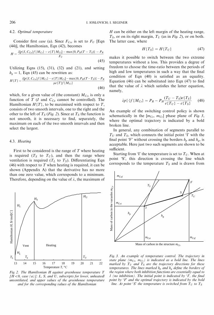
which, for a given value of (the constant) MCs, is only afunction of T (I and CCa cannot be controlled). TheHamiltonian HfTg, to be maximised with respect to T ,consists of two smooth intervals, one to the right and theother to the left of TS (Fig. 2). Since at TS the function isnot smooth, it is necessary to find, separately, themaximum on each of the two smooth intervals and thenselect the largest.

4.3. Heating

First to be considered is the range of T where heatingis required (TS to TU ), and then the range whereventilation is required (TL to TS). Differentiating Eqn(46) with respect to T when heating is required, it can beshown (Appendix A) that the derivative has no morethan one zero value, which corresponds to a minimum.Therefore, depending on the value of l, the maximum of

13 14 15 16 17 18 19 20 21 22

HUHS

HL

TL TUTS

HL

Vent Heating

Temperature T, °C

Ham

ilton

ian

H, $

/mol

[C]

Fig. 2. The Hamiltonian H against greenhouse temperature T[H50, case (a)]; L, S, and U, subscripts for lower, unheated/unventilated, and upper values of the greenhouse temperature

and for the corresponding values of the Hamiltonian

H can be either on the left margin of the heating range,TS, or on its right margin, TU (as in Fig. 2), or on both.The latter case, where

HfTSg ¼ HfTUg ð47Þ

makes it possible to switch between the two extremetemperatures without a loss. This provides a degree offreedom to choose the time-ratio between the periods ofhigh and low temperatures in such a way that the finalcondition of Eqn (40) is satisfied as an equality.Equation (46) can be substituted into Eqn (47) to findthat the value of l which satisfies the latter equation,namely,

lpf�gf fMCsg ¼ PR � PH

ðTU � TSÞefTSgefTUg � efTSg

ð48Þ

An example of the switching control policy is shownschematically in the [mCs, mCv] phase plane of Fig. 3,where the optimal trajectory is indicated by a boldbroken line.

In general, any combination of segments parallel toTU and TS, which connects the initial point ‘I’ with thefinal point ‘F’ without crossing the borders hp and hg, isacceptable. Here just two such segments are shown to besufficient.

Starting from ‘I’ the temperature is set to TU . When atpoint ‘S’, this direction is crossing the line whichcorresponds to the temperature TS and is drawn from

S

hphg

I

F

TU

TS

mCsfmCsi

mCvi

Mass of carbon in the structure mCs

Mas

s of

car

bon

in th

e va

cuol

es m

Cv

Fig. 3. An example of temperature control. The trajectory instate plane (mCs, mCv) is indicated as a bold line. The linesmarked by TU and TS are the trajectory directions for thesetemperatures. The lines marked hp and hg define the borders ofthe region where both inhibition functions are essentially equal to1 (no inhibition). The initial point is indicated by ‘I’, the finalpoint by ‘F’ and the optimal trajectory is indicated by the bold

line. At point ‘S’ the temperature is switched from TU to TS


the final point ‘F’, the temperature is switched to TS

until the final point ‘F’ is reached.Any combination of such zigzag segments, which ends

at the final state, is optimal. This non-unique sequencecan be selected in such a way that the phase trajectorystays in the region of no inhibition. A switching periodof 1 day (option 2 of Section 4�1) is probably shortenough to ensure that inhibition is avoided.

Note that jumping back and forth between TU and TS

is a result of the exponential form of the respirationfunction [Eqn (22)]. The corresponding analysis fora linear respiration function (not shown) yields asingle (intermediate between TU and TS) optimaltemperature.

Since the second term on the right-hand side of Eqn(48) is negative, l must satisfy

lpf�gf f�g � PR50 ð49Þ

From Eqn (48) it is also possible to see that, since l isnon-negative, this regime can exist only if the followinginequality is satisfied:

PR5PHðTU � TSÞefTSgefTUg � efTSg

ð50Þ

which means that when TL5TS and PR is less than theright-hand side in Eqn (50), heating is not justified.

4.4. Ventilation

Since ventilation, between TL and TS, is free ofcharge, the Hamiltonian of Eqn (46) becomes

HfTg ¼l½pf�gf ðMCsg � efTgMCs� � PR

mefTgf fMCsg

¼N

mefTgf fMCsgð51Þ

Removing the constant term lMCs=mf fMCsg anddenoting the resulting numerator N1, the result is

H ¼lpf�gf ðMCsg � PR

mefTgf fMCsg¼

N1

mefTgf fMCsgð52Þ

For l which satisfies

N1 ¼ lpf�gf fMCsg � PR ¼ 0 ð53Þ

any temperature in the feasible range TL4T4TS

maximises the Hamiltonian. This provides the freedomto select a (constant) temperature that satisfies the endcondition, Eqn (40).

4.5. Further points

By now, the following has been established for thevariable spacing case (a) [FCvs ¼ FU ; Eqn (44)].

(1) If heating is required, l should be chosen to satisfyEqn (48), which permits the switching, without loss,between TU and TS, and provides a degree offreedom to satisfy the end condition for the nitratecontent [Eqn (40)].

(2) If ventilation is required, l should be chosen tosatisfy Eqn (53), which makes any temperaturewithin the range TL4T4TS optimal, thus provid-ing a degree of freedom to satisfy the end condition.

If the end condition cannot be satisfied under thiscontrol, then case (b) [N ¼ 0; Eqn (44)] must beconsidered. The numerator of Eqn (42) decreases as T

increases, and since the control FCvs is not definite [Eqn(44)], the temperature control must be on the lowerbound, TL. The value of l is determined from thecondition N ¼ 0 [Eqn (51)], and hence the control FCvs

must be chosen to satisfy the end condition, Eqn (40). Inother words, nitrate supply has to be limited in such away that the end condition is met.

There is no need to consider case (c), because in thiscase nitrate supply is switched off from the verybeginning, which is not realistic and could also beconsidered as a particular control of case (b).

Note that since in this problem the Hamiltonian, Eqn(38), does not depend on the state variable, mCv,satisfying the Pontryagin Maximum Principle (Pontrya-gin et al., 1962) is not only a necessary condition butalso a sufficient condition of optimality.

5. Variable plant spacing: algorithmic solution

The non-uniqueness of the optimal solution maymake it difficult to find a numerical solution without a

priori knowledge of its structure. Since the precedinganalysis revealed the nature of the solution, an appro-priate algorithmic solution, which does not searchexplicitly for the optimal costate value, can be devised.The algorithm can be used to guide a simulation-aidedsearch for the optimal control strategy under constantweather conditions:

(1) Select a crop mass-density MCs, to be maintained ata constant level while searching for the optimalvalues of the controls T and FCvs.

(2) Start with an unlimited nitrate flux (namely FU ) andcontrol heating to switch the temperature back andforth between TU and TS in such a way that leads tomeeting the end condition for mCv (directly obtain-able from mCsf and GNvf ), while avoiding inhibition(e.g. daily cycle).

(3) If the required final mCv cannot be achieved in thatway, keep the temperature on the appropriate levelbetween TS and TL, using ventilation.


(4) If the desired mCvf is still not achievable, keep thetemperature as close as possible to TL, and keepFCvs at an intermediate level between FU and FL (bylimiting the availability of nitrate). Such a solutionis always possible, since FL means zero nitratesupply.

(5) Find the global optimum by searching for theoptimal crop density MCs, repeating steps (1)–(4)for each trial value of MCs.

Note that the algorithm consists of a finite number ofsteps for each point of the MCs grid and thus is a finiteprocedure.

6. Variable spacing: free final size

For situations where lettuce is harvested not at a pre-specified size but at a time which maximises the profit tothe grower, the optimisation criterion needs to bemodified. When the final state is free, the market price,which did not appear in the original minimisationcriterion [Eqn (35)], needs to be specified as a function ofthe head size. The price per unit mass of head is often aconcave (downward) function of head size PmfmCsg andit is assumed here that it is invariant with time. Theappropriate maximisation criterion has, thus, the form

J ¼PmfmCsftf ggmCsftf g

�Z tf

ti

aftg½maxf0;PH ðT � TSÞg þ PR� dt ð54Þ

The final time tf , and the final size mCsftf g are bothinitially unknown, and the problem is a so-called mixedoptimal control problem (Elsgolc, 1961). The criterion[Eqn (54)] can be written in an equivalent integralLagrange form, utilizing Eqn (29), as

J ¼Z tf

ti

aftgFCvs

dPm

dmCs

mCs þ Pm

� ��

�aftg½maxf0;PH ðT � TSÞg þ PR�Þ dt ð55Þ

Using mCs as an independent variable, the correspond-ing Hamiltonian, similar to the original one [Eqn (38)]becomes

H ¼dPmfmCsg

dmCs

mCs þ PmfmCsg� �

þ lFCp � FCm

FCvs

� ð1 þ yÞ� �

�1

FCvs

½maxf0;PH ðT � TSÞg þ PR� ð56Þ

The additional (first) term depends only on mCs and noton the controls T , afmCsg and FCvs. Thus, the analysisleading to the optimal control proceeds in the same way

as before. The difference is that the optimal value of theadditional parameter mCsftf g, must be found. Thecorresponding final constraint is

mCvfmCsf g5gmCsf ð57Þ

and transversality condition for this final constraint hasthe following form (Seierstad & Sydsaeter, 1987):

HfmCsf g ¼ gl ð58Þ

In these constraints, the constant g (ratio between finalvalues of state variables) is such that the final nitrateconcentration is low enough to satisfy the requirements.

The transversality condition can be combined withEqn (56) at the final point to obtain

dPmfmCsf gdmCs

mCsf þ PmfmCsf g

¼ gl� lFCp � FCm

FCvs

� ð1 þ yÞ� �

þ1

FCvs

½maxf0;PH ðT � TSÞg þ PR� ð59Þ

The costate variable l for the assumed current value ofMCs is determined in the same way as before, namelyfrom Eqn (48) for heating and from Eqn (53) forventilation. For the case of a limited nitrate supply, l isdetermined from T ¼ TL and the condition N ¼ 0 [Eqn(51)], also as before. The final value mCsf has to be foundfrom Eqn (59) when the final constraint in Eqn (57) issatisfied as an equality. Note that when MCs is changedin the process of maximisation of H of Eqn (56), thevalues of l and of mCsf are changed as well.

7. Constant plant spacing

When plants cannot be respaced, which is stillgenerally true for greenhouses, the model, problemformulation, optimisation criterion and Hamiltonianare all the same as for the variable-spacing situation.The difference is in the now more limited set of controlvariables, consisting only of temperature T , and nitrateflux (replaced, as before, by FCvs). This difference turnsout to have a significant effect on the nature of thesolution. The analysis for the case of a fixed final state istaken up first, and the case of a free final size is treatedin Section 7�6.

The assumptions and analysis of the fixed-final-statecase are the same as for the variable spacing (Section 3).The area per plant a, is however now a constant, andMCs can be expressed, in view of Eqn (27), as mCs=a,which monotonically increases as the plants grow. Thus,the Hamiltonian is a function of the control variablesand of the independent variable mCs.


When MCs is small, it can be seen from Eqns (42) and(43) that N is likely to be negative. Therefore, case (a)[Eqn (44)] is considered first. Since in this case FCvs is setto FU , the relevant Hamiltonian is Eqn (46). Theproblem, as before, is to find the value of T whichmaximises H.

7.1. Heating

First to be considered is the range of T where heatingis required (TS to TU ). Again, depending on the valuesof l and MCs, the maximum of H can be either on theleft margin TS, or on the right margin TU , or on both(Fig. 2). It is now required to find whether the differenced HfTSg2HfTUg increases or decreases as the plantsgrow (as mCs, and hence MCs, increases).

The difference d can be written, in view of Eqn (46), as

d HfTSg � HfTUg ¼ A þ B

lpf�g1

mefTSg�

1

mefTUg

� �

þ1

mf fMCsgPH

ðTU � TSÞefTUg

� ��

�PR1

efTSg�

1

efTUg

� ��ð60Þ

where the first term A, which is proportional to l, isalways positive [l > 0, Eqn (41)]; pf�g > 0, Eqn (20);TU > TS], and only the second term B is a function ofMCs. Depending on the prevailing price structure, theconstant bracketed factor in B is either positive ornegative. If it is negative (high PR=PH ), B is negative(since mf fMCsg is always positive), and vice versa.

Differentiating d with respect to MCs results in

@d@MCs

¼@B

@MCs

¼ �B

f fMCsg@f fMCsg@MCs

ð61Þ

First to be considered is the situation where B is negative(low cost of heat). Since @f fMCsg=@MCs [Eqn (23)] ispositive and B is negative, it follows from Eqn (61) that@d=@MCs is positive and d increases with MCs and thuswith time (a is constant). When the crop is young,f fMCsg in the denominator of B [Eqn (60)] is small, B islarge negative, and although A is positive, it is likely thatd50, which means that the optimum is at T ¼ TU andheating is justified. As the crop matures, d increases andmay become positive, which would switch the optimaltemperature to TS (no heating and no ventilation). Nointermediate values of T are optimal under ourassumptions, which means that the control is bang-bang. Since @d=@MCs [Eqn (61)] is always positive, onced becomes positive, it will never become negative again

and the maximum of the Hamiltonian in the TS to TU

temperature range will remain on the left margin TS

(Fig. 2).In summary, the high temperature TU , is valid on the

interval

MCsi4MCs4MCs1 ð62Þ

where MCsi and MCs1 are the initial value of MCs and thevalue that satisfies Eqn (47) ðd HfTSg2HfTUg ¼ 0Þfor a given value of l. When MCs1 is reached, TU

switches to TS, which means that heating will no longerbe required (Fig. 4). Note that for certain values of l,MCs1 may be less than MCsi, implying that T ¼ TS fromthe beginning (no heating). In general, if the cost of heatis sufficiently high relative to the cost of rent to make B

positive, d is never negative, the maximum value of theHamiltonian is attained for T ¼ TS, and heating is notjustified.

7.2. Ventilation for the upper bound carbon flux

to the structure

The appropriate Hamiltonian for ventilation, Eqn(51), can be written as

H ¼N

mefTgf fMCsg

¼lpf�gf fMCsg � PR

mefTgf fMCsg�

lMCs

mf fMCsg

¼N1

mefTgf fMCsg�

lMCs

mf fMCsgð63Þ

where N1 is the same as in Eqn (52). Suppose that MCs

has reached MCs1, where d ¼ 0 and the numerator N isnegative [case (a)], while N1 is still negative. As long asN150, TS remains the optimal temperature [Eqn (63)],but as soon as N1 becomes positive, the optimaltemperature switches to TL [Eqn (63)] and remainsthere for ever after, even if N becomes eventuallypositive (Fig. 4). The value of MCs at the switching pointof N1 (where N1 ¼ 0) is denoted by MCs2, namely [Eqn(52)]

f fMCs2g ¼ PR=lpf�g ð64Þ

Note that MCs2 may be smaller than MCs1 if rent is veryinexpensive.

7.3. Ventilation for the lower bound carbon flux

to the structure

Since the analysis in Appendix B shows that case (b) isnot feasible for constant spacing, case (c) is considered

TU

TS

TL

FU

FL

0

δN1

N MCsi MCsfMCs1 MCs2 MCs3 MCs4case acase ccase a

Mass of carbon content in the structure MCs

Heat

Vent

AbundantnitrateZero

nitrate

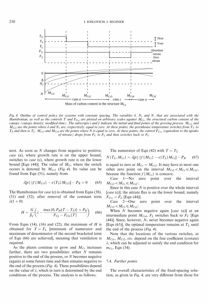
Fig. 4. Outline of control policy for systems with constant spacing. The variables d, N1 and N, that are associated with theHamiltonian, as well as the controls T and FCvs are plotted on arbitrary scales against MCs, the structural carbon content of thecanopy (canopy density, modified time). The subscripts i and f indicate the initial and final points of the growing process. MCs1 andMCs2 are the points where d and N1 are, respectively, equal to zero. At these points, the greenhouse temperature switches from TU toTS and then to TL. MCs3 and MCs4 are the points where N is equal to zero. At these points, the control FCvs (equivalent to the uptake

of nitrate) drops from FU to FL and then switches back to FU


next. As soon as N changes from negative to positive,case (a), where growth rate is on the upper bound,switches to case (c), where growth rate is on the lowerbound [Eqn (44)]. The value of MCs where the switchoccurs is denoted by MCs3 (Fig. 4). Its value can befound from Eqn (51), namely from

l½pf�gf fMCs3g � efTSgMCs3� � PR ¼ 0 ð65Þ

The Hamiltonian for case (c) is obtained from Eqns (38),(31) and (32), after removal of the constant termlð1 þ yÞ:

H ¼G

bC

l�maxf0;PH ðT � TSÞg þ PR

FCp � FCmfTg

� �ð66Þ

From Eqns (14), (16) and (22), the maximum of H isobtained for T ¼ TL [minimum of numerator andmaximum of denominator of the second bracketed termof Eqn (66) are achieved], meaning that ventilation isrequired.

As the plants continue to grow and MCs increasesfurther, there are two possibilities: either N remainspositive to the end of the process, or N becomes negative(again) at some future time and then remains negative tothe end of the process (Fig. 4). These possibilities dependon the value of l, which in turn is determined by the endconditions of the process. The analysis is as follows.

The numerator of Eqn (42) with T ¼ TL

NfTL;MCsg ¼ l½pf�gf fMCsg � efTLgMCs� � PR ð67Þ

is equal to zero at MCs ¼ MCs3. It may have at most oneother zero point on the interval MCs35MCs4MCsf ,because the function f fMCsg is concave.

Case 1}No zero point over the intervalMCs35MCs4MCsf :

Since in this case N is positive over the whole interval[case (c)], the nitrate flux is on the lower bound, namelyFCvs ¼ FL [Eqn (44)].

Case 2}One zero point over the intervalMCs35MCs4MCsf :

When N becomes negative again [case (a)] at anintermediate point MCs4, FL switches back to FU [Eqn(44)]. Since, however, N1 never becomes negative again[Eqn (63)], the optimal temperature remains at TL untilthe end of the process (Fig. 4).

Note that the locations of the various switches, atMCs1, MCs2, etc. depend on the free coefficient (costate)l, which can be adjusted to satisfy the end condition formCv, Eqn (34).

7.4. Further points

The overall characteristics of the fixed-spacing solu-tion, as given in Fig. 4, are very different from those for


variable-spacing systems, where the optimal control isinvariant with time. Here, as in other optimisationstudies of plants at fixed spacing (Marsh & Albright,1991; Seginer & McClendon, 1992), the recommendedtemperature decreases as the crop matures. The mainreason is the advantage of closing the canopy (absorbingall the available light) at an early stage. In the presentstudy, an initially higher temperature promotes growthand leads to an earlier canopy closure, albeit at theexpense of a higher nitrate content. As soon as thecanopy closes, there is less advantage in rapid growthand the lower temperatures make it possible to reducethe nitrate concentration to an acceptable level. Redu-cing the availability of nitrate by jumping down from FU

to FL at MCs3, agrees with the intuitive strategy thatinitially an effort must be made to close the canopy asfast as possible and postpone the adjustment of nitrateconcentration to the linear growth phase (Seginer et al.,1999). The jump back to FU at MCs4 is less intuitive andmay not always be required. The minimum betweenMCs3 and MCs4 may be associated with a maximum ofnet photosynthesis.

The optimal control solutions are based on theassumption that the inhibition functions are inactive.Unlike the case of variable spacing, where frequentswitching between TU and TS is helpful in balancing thecontent of the vacuole, it is not clear how to preventimbalance with the fixed-spacing strategy. Longstretches with high temperature TU , may reduce thecarbon content of the vacuole GCv to a sufficiently lowlevel, which may activate growth inhibition [Eqn (25)].Long stretches of low temperature may result inphotosynthesis inhibition [Eqn (24)]. This solution,which is based on simplifying assumptions, is notintended to produce final quantitative solutions to theoptimal control problem. Rather, it is meant to providea general guideline to numerical solutions, which wouldbe based on the complete model (including activeinhibitions) and applied to a variable weather. InSection 8, a numerical example is presented, whichindicates that a constant intermediate temperature mayproduce an outcome that is only slightly inferior to theoptimal.

7.5. An algorithmic solution

The algorithm consists of a one-dimensional searchover the non-negative coefficient (costate) l. Thecontrols T and FCvs are only changed at the pointsMCs1, MCs2, MCs3 and MCs4, if these points exist. Thelocation of these points depends on the environment, theprices, the end condition and on the value of l. A proper

value of l is that which satisfies the end condition ofEqn (40) as an equality.

7.6. Free final size

The free final-size problem is also relevant toconstant-spacing systems. The solution may be obtainedby solving the constant spacing, fixed-final-state pro-blem, for a range of final head sizes. The solution whichmaximises the criterion of Eqn (54) is the desired one.An alternative is to use the transversality condition, Eqn(59). The algorithmic solution of Section 7�5 is applic-able here too. The difference is that the final state mCsf

for the current value of l is determined from theconstraint in Eqn (57) taken as an equality. In addition,the value of l must be corrected iteratively in such a waythat the transversality condition of Eqn (59) is satisfied.

8. Sample numerical solutions for problems witha fixed final state

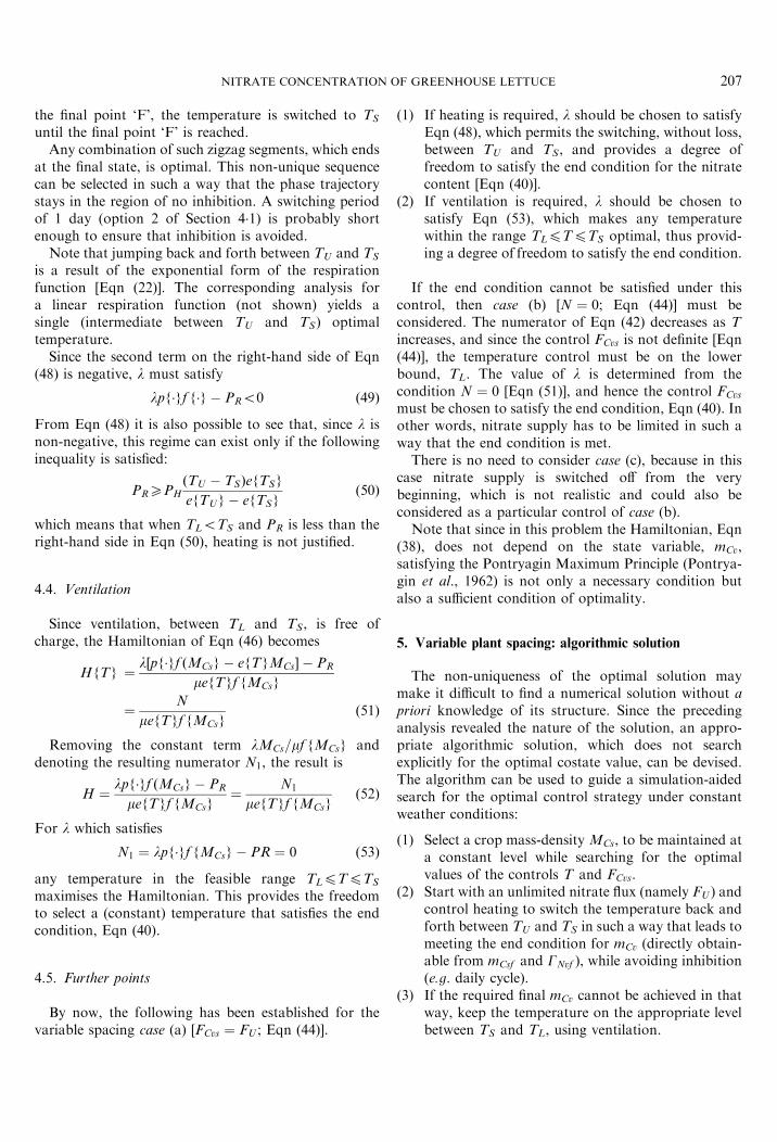
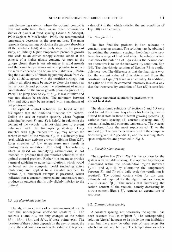
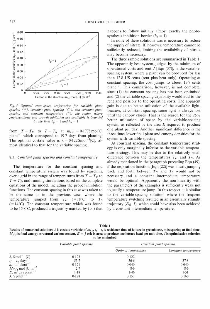
The algorithmic solutions of Sections 5 and 7�5 wereused to find the optimal trajectories for lettuce grown toa fixed final state in three different growing systems: (1)variable plant spacing, (2) constant spacing and (3)constant spacing and constant temperature. The systemsare ordered from the most sophisticated (1) to thesimplest (3). The parameter values used in the computa-tions are given in Appendix C, and the resulting state-space trajectories are presented in Fig. 5.

8.1. Variable plant spacing

The step-like line (r) in Fig. 5 is the solution for thesystem with variable spacing. The optimal trajectory ismaintained within the no-inhibition region (betweenhp ¼ 1 and hg ¼ 1) by alternating the temperaturebetween TU and TS on a daily cycle (no ventilation isrequired). The optimal costate value for this case,although not required for the algorithmic solution, isl ¼ 0�123 $mol�1[C]. This means that increasing thecarbon content of the vacuole, namely decreasing itsnitrate content [Eqn (13)], requires an expenditure ofresources.

8.2. Constant plant spacing

A constant spacing, not necessarily the optimal, hasbeen selected: a ¼ 0�04m2 plant�1. The correspondingsolution (circles) happens to lie inside the non-inhibitionarea, but there may be other sets of parameters forwhich this will not be true. The temperature switches

0 0.05 0.10 0.15 0.20 0.25 0.30 0.350

0.02

0.04

0.06

0.08

0.10

0.12

0.14

0.16

0.18

Carbon in the structure mCs, mol [C ] plant_1

Car

bon

in th

e va

cuol

es m

Cv,

mol

[C

] pl

ant_ 1

1

hg = 1

hp = 1

Fig. 5. Optimal state-space trajectories for variable plantspacing (,), constant plant spacing (*), and constant plantspacing and constant temperature (*); the region wherephotosynthesis and growth inhibition are negligible is bounded

by the lines hp ¼ 1 and hg ¼ 1


from T ¼ TU to T ¼ TS at mCs1 ¼ 0�1778mol[C]plant�1 which correspond to 19�7 days from planting.The optimal costate value is l ¼ 0�122 $mol�1[C], al-most identical to that for the variable spacing.

8.3. Constant plant spacing and constant temperature

The temperature for the constant spacing andconstant temperature system was found by searchingover a grid in the range of temperatures from T ¼ TU toT ¼ TS, and running simulations based on the completeequations of the model, including the proper inhibitionfunctions. The constant spacing in this case was taken tobe the same as in the previous case, where thetemperature jumped from TU (=188C) to TS

(=148C). The constant temperature which was foundto be 15�88C, produced a trajectory marked by (� ) that

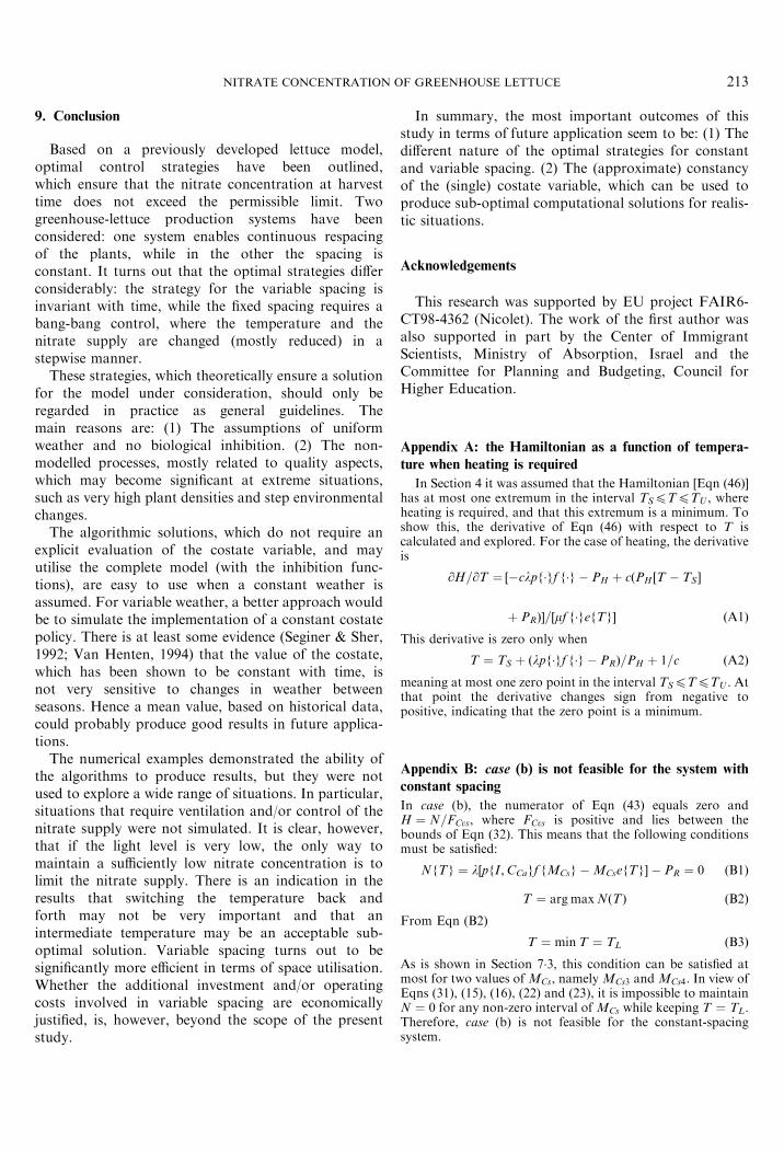
Table

Results of numerical solutions: l is costate variable of mCv, tf� ti is

MCsf is final canopy structural carbon content, E ¼R

a dt is area to

to be min

Variable plant spacing

l, $mol�1 [C] 0�123tf � ti, days 53�7af , m2 plant�1 0�121MCsf , mol [C] m–2 2�7E, m2 day plant�1 1�18J, $ plant�1 0�128

happens to follow initially almost exactly the photo-synthesis inhibition border ðhp ¼ 1Þ.

In none of these solutions was it necessary to reducethe supply of nitrate. If, however, temperature cannot besufficiently reduced, limiting the availability of nitratemay become necessary.

The three sample solutions are summarised in Table 1.The apparently best system, judged by the minimum ofoperational costs and rent J [Eqn (37)], is the variable-spacing system, where a plant can be produced for lessthan 12�8 US cents (rent plus heat only). Operating atconstant spacing, the cost jumps to about 15�7 centsplant�1. This comparison, however, is not complete,since (1) the constant spacing has not been optimisedand (2) the variable-spacing capability would add to therent and possibly to the operating costs. The apparentgain is due to better utilisation of the available light,because, at constant spacing, some light is always lostuntil the canopy closes. That is the reason for the 25%better utilisation of space by the variable-spacingsystem, as reflected by the area E required to produceone plant per day. Another significant difference is thethree times lower final plant and canopy densities for thesystem with variable spacing.

At constant spacing, the constant temperature strat-egy is only marginally inferior to the variable tempera-ture strategy. This may be due to the relatively smalldifference between the temperatures TU and TS. Asalready mentioned in the paragraph preceding Eqn (49),if the respiration function [Eqn (22)] was linear, jumpingback and forth between TU and TS would not benecessary and a constant intermediate temperaturewould be optimal. Apparently the non-linearity withthe parameters of the examples is sufficiently weak notto justify a temperature jump. In this respect, it is similarto the variable-spacing solution, where the frequenttemperature switching resulted in an essentially straighttrajectory (Fig. 5), which could have also been achievedby a constant intermediate temperature.

1

residence time of lettuce in greenhouse, af is spacing at final time,

produce one lettuce head per unit time, J is optimisation criterion

imised

Constant plant spacing

Optimal temperature Constant temperature

0�12236�6 37�8

0�040 0�0408�6 8�6

1�46 1�510�157 0�160


9. Conclusion

Based on a previously developed lettuce model,optimal control strategies have been outlined,which ensure that the nitrate concentration at harvesttime does not exceed the permissible limit. Twogreenhouse-lettuce production systems have beenconsidered: one system enables continuous respacingof the plants, while in the other the spacing isconstant. It turns out that the optimal strategies differconsiderably: the strategy for the variable spacing isinvariant with time, while the fixed spacing requires abang-bang control, where the temperature and thenitrate supply are changed (mostly reduced) in astepwise manner.

These strategies, which theoretically ensure a solutionfor the model under consideration, should only beregarded in practice as general guidelines. Themain reasons are: (1) The assumptions of uniformweather and no biological inhibition. (2) The non-modelled processes, mostly related to quality aspects,which may become significant at extreme situations,such as very high plant densities and step environmentalchanges.

The algorithmic solutions, which do not require anexplicit evaluation of the costate variable, and mayutilise the complete model (with the inhibition func-tions), are easy to use when a constant weather isassumed. For variable weather, a better approach wouldbe to simulate the implementation of a constant costatepolicy. There is at least some evidence (Seginer & Sher,1992; Van Henten, 1994) that the value of the costate,which has been shown to be constant with time, isnot very sensitive to changes in weather betweenseasons. Hence a mean value, based on historical data,could probably produce good results in future applica-tions.

The numerical examples demonstrated the ability ofthe algorithms to produce results, but they were notused to explore a wide range of situations. In particular,situations that require ventilation and/or control of thenitrate supply were not simulated. It is clear, however,that if the light level is very low, the only way tomaintain a sufficiently low nitrate concentration is tolimit the nitrate supply. There is an indication in theresults that switching the temperature back andforth may not be very important and that anintermediate temperature may be an acceptable sub-optimal solution. Variable spacing turns out to besignificantly more efficient in terms of space utilisation.Whether the additional investment and/or operatingcosts involved in variable spacing are economicallyjustified, is, however, beyond the scope of the presentstudy.

In summary, the most important outcomes of thisstudy in terms of future application seem to be: (1) Thedifferent nature of the optimal strategies for constantand variable spacing. (2) The (approximate) constancyof the (single) costate variable, which can be used toproduce sub-optimal computational solutions for realis-tic situations.

Acknowledgements

This research was supported by EU project FAIR6-CT98-4362 (Nicolet). The work of the first author wasalso supported in part by the Center of ImmigrantScientists, Ministry of Absorption, Israel and theCommittee for Planning and Budgeting, Council forHigher Education.

Appendix A: the Hamiltonian as a function of tempera-

ture when heating is required

In Section 4 it was assumed that the Hamiltonian [Eqn (46)]has at most one extremum in the interval TS4T4TU , whereheating is required, and that this extremum is a minimum. Toshow this, the derivative of Eqn (46) with respect to T iscalculated and explored. For the case of heating, the derivativeis

@H=@T ¼ ½�clpf�gf f�g � PH þ cðPH ½T � TS�

þ PRÞ�=½mf f�gefTg� ðA1Þ

This derivative is zero only when

T ¼ TS þ ðlpf�gf f�g � PRÞ=PH þ 1=c ðA2Þ

meaning at most one zero point in the interval TS4T4TU . Atthat point the derivative changes sign from negative topositive, indicating that the zero point is a minimum.

Appendix B: case (b) is not feasible for the system with

constant spacing

In case (b), the numerator of Eqn (43) equals zero andH ¼ N=FCvs, where FCvs is positive and lies between thebounds of Eqn (32). This means that the following conditionsmust be satisfied:

NfTg ¼ l½pfI ;CCagf fMCsg � MCsefTg� � PR ¼ 0 ðB1Þ

T ¼ arg max NðTÞ ðB2Þ

From Eqn (B2)

T ¼ min T ¼ TL ðB3Þ

As is shown in Section 7�3, this condition can be satisfied atmost for two values of MCs, namely MCs3 and MCs4. In view ofEqns (31), (15), (16), (22) and (23), it is impossible to maintainN ¼ 0 for any non-zero interval of MCs while keeping T ¼ TL.Therefore, case (b) is not feasible for the constant-spacingsystem.


Appendix C: parameter values for numerical examples

Environmental conditions:

TL ¼ 88C

TS ¼ 148C

TU ¼ 188C

I ¼ 10 mol½PAP� day�1

(abbreviation PAP stands for photosynthetically activephotons).

Prices:

PH ¼ 3 � 10�3 $m�2 d�1 K�1 ðcost of heatingÞ

PR ¼ 0�1 $m�2 d�1 ðcost of rentÞ

Photosynthesis:

e ¼ 0�07 mol½C�mol�1½phot�

s ¼ 1�4� 10�3 m s�1

Respiration and growth:

y ¼ 0�3

m ¼ 17

k ¼ 0�25 � 10�6 mol½C� ðm2½ground� sÞ�1

c ¼ 0�0693 1=K

Photosynthesis and growth:

c ¼ 1�7 m2 mol�1½C�

Internal relationships:

bN ¼ 6�0 kPa m3 mol�1½N�

bC ¼ 0�61 kPa m3 mol�1½C�

a ¼ 0�741 � 10�3 m3 mol�1½C�

P ¼ 580 kPa

Inhibition functions:

bp ¼ 0�8

sp ¼ 40

bg ¼ 0�2

sg ¼ 40

Nitrogen-to-carbon ratio in the structure:

rNs ¼ 0�08 g½N� g�1½C�

Spacing:

a ¼ 0�04 m2½ground� plant�1

Initial conditions:

mCvi ¼ 1�7� 10�4 mol½C� plant�1

mCSi ¼ 5�1 � 10�4 mol½C� plant�1

Final conditions:

mCvf ¼ 0�10 mol½C� plant�1

mCsf ¼ 0�34 mol½C� plant�1

These final conditions correspond to harvested lettuce headshaving fresh weight of 0�3 kg plant�1, and to nitrate concen-tration at the time of harvest of 3500 p.p.m.

Arbitrarily fixed:

T� ¼ 208C1

References

Both A J; Albright L D; Langhans R W (1999). Designof a demonstration greenhouse operation for commercialhydroponic lettuce production. ASAE Paper No. 99-4123

Drews M; Schonhof I; Krumbein A (1995). Influence of growthseason on the content of nitrate, vitamin C, b-Carotene andsugar of head lettuce under greenhouse conditions. Garten-bauwissenschaft, 60(4), 180–187

Elsgolc L E (1961). Calculus of Variations. Pergamon Press,London

Goto E; Albright L D; Langhans R W; Leed A R (1994). Plantspacing management in hydroponic lettuce production.ASAE Paper No. 94-4574

Ioslovich I; Gutman P -O (2000). Plant factory optimisation.Automatica, 36(11), 1665–1668

MAFF (1997). 1996/97 UK monitoring program for nitrate inlettuce and spinach. Ministry of Agriculture, Fisheries andFood, Food Surveillance Information Sheet, No 121, pp.1–10. HMSO, UK

Marsh L S; Albright L D (1991). Economically optimum daytemperatures for greenhouse hydroponic lettuce production,part I: a computer model. Transactions of the ASAE, 34(2),550–556

Pontryagin L S; Boltyanskii V G; Gamkrelidze R V;

Mishchenko E F (1962). The Mathematical Theory ofOptimal Processes. Wiley-Interscience, New York

Prince R P; Bartok J W Jr (1978). Plant spacing for controlledenvironment plant growth. Transactions of the ASAE, 21,

332–336Prince R P; Bartok J W Jr; Protheroe D W Jr (1981). Lettuce

production in a controlled environment plant growth unit.Transactions of the ASAE, 24(3), 725–730

Seginer I; Ioslovich I (1999). Optimal spacing and cultivationintensity for an industrialized crop production system.Agricultural Systems, 62, 143–157

Seginer I; McClendon R W (1992). Methods for optimalcontrol of the greenhouse environment. Transactions of theASAE, 35(4), 1299–1307

Seginer I; Sher A (1992). Neural-nets for greenhouse climatecontrol. ASAE Paper No. 92-7013


Seginer I; Buwalda F; van Straten G (1998). Nitrate concentra-tion in greenhouse lettuce: a modelling study. ActaHorticulturae, 456, 189–197

Seginer I; van Straten G; Buwalda F (1999). Lettuce growthlimited by nitrate supply. Acta Horticulturae, 507,

141–148

Seierstadt A; Sydsaeter K (1987). Optimal Control Theory withEconomic Applications. Elsevier Science Publishers, Am-sterdam

Van Henten E J (1994). Greenhouse climate management: anoptimal control approach. Doctor Dissertation, Wagenin-gen Agricultural University, The Netherlands

Documents

SE—Structures and Environment: Acceptable Nitrate Concentration of Greenhouse Lettuce: Two Optimal Control Policies