Computers & Graphics 35 (2011) 904–915

Contents lists available at ScienceDirect

Computers & Graphics

0097-84

doi:10.1

� Corr

E-m

journal homepage: www.elsevier.com/locate/cag

Technical Section

Shape classification and normal estimation for non-uniformly sampled, noisypoint data

Cindy Grimm �, William D. Smart

Campus Box 1045, Department of Computer Science and Engineering, Washington University in St. Louis, St. Louis, MO 63130, United States

a r t i c l e i n f o

Article history:

Received 8 October 2010

Received in revised form

11 March 2011

Accepted 17 March 2011Available online 13 April 2011

Keywords:

Surface reconstruction

Normal estimation

Shape classification

Unlabeled data

Point data

One-ring

93/$ - see front matter & 2011 Elsevier Ltd. A

016/j.cag.2011.03.036

esponding author.

ail addresses: cmg@wustl.edu (C. Grimm), wd

a b s t r a c t

We present an algorithm for robustly analyzing point data arising from sampling a 2D surface

embedded in 3D, even in the presence of noise and non-uniform sampling. The algorithm outputs,

for each data point, a surface normal, a local surface approximation in the form of a one-ring, the local

shape (flat, ridge, bowl, saddle, sharp edge, corner, boundary), the feature size, and a confidence value

that can be used to determine areas where the sampling is poor or not surface-like.

We show that the normal estimation out-performs traditional fitting approaches, especially when

the data points are non-uniformly sampled and in areas of high curvature. We demonstrate surface

reconstruction, parameterization, and smoothing using the one-ring neighborhood at each point as an

approximation of the full mesh structure.

& 2011 Elsevier Ltd. All rights reserved.

1. Introduction

We present an algorithm for estimating surface normals andlocal shape from point data that is sampled from a 2D surfaceembedded in 3D space. We show that our algorithm is robust inthe presence of both noise and non-uniform sampling. For eachdata point the algorithm produces a surface normal, a localsurface approximation in the form of a one-ring, a local estimateof shape (flat, bowl, saddle, ridge, edge, corner, or boundary), ameasure of the feature size, and a confidence value. This valuereflects both the quality of the local sampling and noise in thefunction and can be used to detect places where the points do notrepresent a surface. The one-ring neighborhood can be used forfurther mesh processing such as reconstruction, smoothing orspectral mesh processing.

Traditional normal estimation approaches usually rely on fitting alocal surface approximation to some subset of the k-nearest neigh-bors [1]. This approach works well most of the time, but it has severallimitations (see Fig. 1). First, if the data are non-uniformly distributed,the fitting error becomes biased—the classic example of this iscontour data, where the best planar fit can be perpendicular to thesurface. Second, the local surface approximation may not haveenough flexibility to match the surface, which introduces additionalerror and increases the sensitivity to non-uniformly distributed data.

ll rights reserved.

s@wustl.edu (W.D. Smart).

Increasing the flexibility of the representation, unfortunately, can leadto over-fitting. Third, there is no method for distinguishing betweennoisy data and poor local fit, or determining if the local samples evenrepresent a surface.

Our fundamental idea is to build three different representa-tions of the local surface—a surface normal, a good-quality one-ring, and a local shape model—and cross-validate them. If allthree representations are mutually consistent with each other and

the data, then we can be reasonably confident that they arecorrect. In this we are closer in spirit to approaches that userobust statistics [2,3]. We also gain a lot of information about thesamples, namely how much noise is present, how even thesampling is, if there are sharp features or boundaries, the localfeature size, and a plausible graph structure. There are severalapproaches that use one of these pieces of information to derive

another—for example, normals from the graph structure [4]—butto our knowledge no-one else has used cross-validation toimprove normal estimation and surface analysis.

We show that cross-validation produces better-quality nor-mals than standard fitting approaches, particularly in areas withuneven sampling and high curvature. Not only are the averagesbetter, but the variance is narrower, meaning we are less likely toreturn a ‘‘wrong’’ result. This is particularly true in saddle andridge areas. Our approach also behaves well near boundaries andsharp features, and can explicitly identify them.

We make use of three observations. The first is that, locally,smooth surfaces are either flat (zero curvature), ridges (zerocurvature in one direction), bowls (positive curvature), or saddles

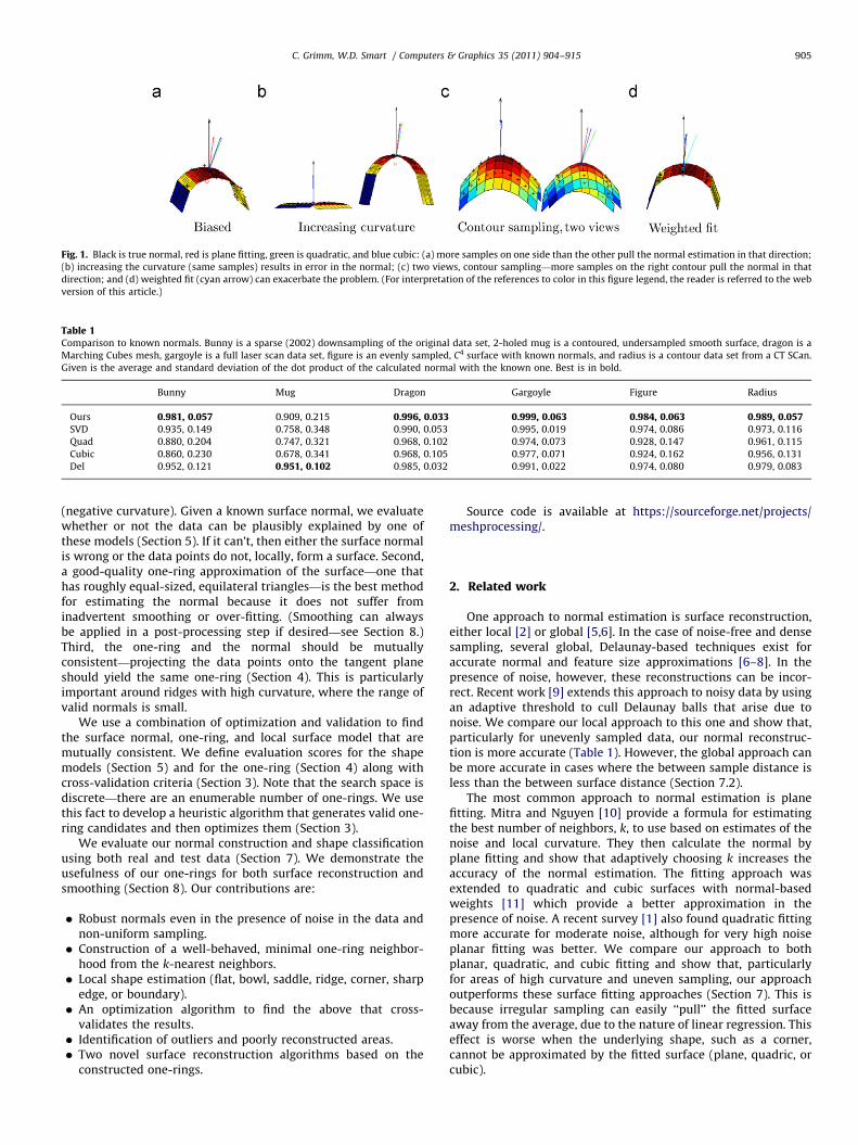
Fig. 1. Black is true normal, red is plane fitting, green is quadratic, and blue cubic: (a) more samples on one side than the other pull the normal estimation in that direction;

(b) increasing the curvature (same samples) results in error in the normal; (c) two views, contour sampling—more samples on the right contour pull the normal in that

direction; and (d) weighted fit (cyan arrow) can exacerbate the problem. (For interpretation of the references to color in this figure legend, the reader is referred to the web

version of this article.)

Table 1Comparison to known normals. Bunny is a sparse (2002) downsampling of the original data set, 2-holed mug is a contoured, undersampled smooth surface, dragon is a

Marching Cubes mesh, gargoyle is a full laser scan data set, figure is an evenly sampled, C4 surface with known normals, and radius is a contour data set from a CT SCan.

Given is the average and standard deviation of the dot product of the calculated normal with the known one. Best is in bold.

Bunny Mug Dragon Gargoyle Figure Radius

Ours 0.981, 0.057 0.909, 0.215 0.996, 0.033 0.999, 0.063 0.984, 0.063 0.989, 0.057SVD 0.935, 0.149 0.758, 0.348 0.990, 0.053 0.995, 0.019 0.974, 0.086 0.973, 0.116

Quad 0.880, 0.204 0.747, 0.321 0.968, 0.102 0.974, 0.073 0.928, 0.147 0.961, 0.115

Cubic 0.860, 0.230 0.678, 0.341 0.968, 0.105 0.977, 0.071 0.924, 0.162 0.956, 0.131

Del 0.952, 0.121 0.951, 0.102 0.985, 0.032 0.991, 0.022 0.974, 0.080 0.979, 0.083

C. Grimm, W.D. Smart / Computers & Graphics 35 (2011) 904–915 905

(negative curvature). Given a known surface normal, we evaluatewhether or not the data can be plausibly explained by one ofthese models (Section 5). If it can’t, then either the surface normalis wrong or the data points do not, locally, form a surface. Second,a good-quality one-ring approximation of the surface—one thathas roughly equal-sized, equilateral triangles—is the best methodfor estimating the normal because it does not suffer frominadvertent smoothing or over-fitting. (Smoothing can alwaysbe applied in a post-processing step if desired—see Section 8.)Third, the one-ring and the normal should be mutuallyconsistent—projecting the data points onto the tangent planeshould yield the same one-ring (Section 4). This is particularlyimportant around ridges with high curvature, where the range ofvalid normals is small.

We use a combination of optimization and validation to findthe surface normal, one-ring, and local surface model that aremutually consistent. We define evaluation scores for the shapemodels (Section 5) and for the one-ring (Section 4) along withcross-validation criteria (Section 3). Note that the search space isdiscrete—there are an enumerable number of one-rings. We usethis fact to develop a heuristic algorithm that generates valid one-ring candidates and then optimizes them (Section 3).

We evaluate our normal construction and shape classificationusing both real and test data (Section 7). We demonstrate theusefulness of our one-rings for both surface reconstruction andsmoothing (Section 8). Our contributions are:

�

Robust normals even in the presence of noise in the data andnon-uniform sampling. � Construction of a well-behaved, minimal one-ring neighbor-

hood from the k-nearest neighbors.

� Local shape estimation (flat, bowl, saddle, ridge, corner, sharp

edge, or boundary).

� An optimization algorithm to find the above that cross-

validates the results.

� Identification of outliers and poorly reconstructed areas. � Two novel surface reconstruction algorithms based on the

constructed one-rings.

Source code is available at https://sourceforge.net/projects/

meshprocessing/.

2. Related work

One approach to normal estimation is surface reconstruction,either local [2] or global [5,6]. In the case of noise-free and densesampling, several global, Delaunay-based techniques exist foraccurate normal and feature size approximations [6–8]. In thepresence of noise, however, these reconstructions can be incor-rect. Recent work [9] extends this approach to noisy data by usingan adaptive threshold to cull Delaunay balls that arise due tonoise. We compare our local approach to this one and show that,particularly for unevenly sampled data, our normal reconstruc-tion is more accurate (Table 1). However, the global approach canbe more accurate in cases where the between sample distance isless than the between surface distance (Section 7.2).

The most common approach to normal estimation is planefitting. Mitra and Nguyen [10] provide a formula for estimatingthe best number of neighbors, k, to use based on estimates of thenoise and local curvature. They then calculate the normal byplane fitting and show that adaptively choosing k increases theaccuracy of the normal estimation. The fitting approach wasextended to quadratic and cubic surfaces with normal-basedweights [11] which provide a better approximation in thepresence of noise. A recent survey [1] also found quadratic fittingmore accurate for moderate noise, although for very high noiseplanar fitting was better. We compare our approach to bothplanar, quadratic, and cubic fitting and show that, particularlyfor areas of high curvature and uneven sampling, our approachoutperforms these surface fitting approaches (Section 7). This isbecause irregular sampling can easily ‘‘pull’’ the fitted surfaceaway from the average, due to the nature of linear regression. Thiseffect is worse when the underlying shape, such as a corner,cannot be approximated by the fitted surface (plane, quadric, orcubic).

C. Grimm, W.D. Smart / Computers & Graphics 35 (2011) 904–915906

Pauly et al. [12] present a modification of the plane-fittingalgorithm that weights points by their distance from the point ofinterest. This is called locally weighted regression in the machinelearning literature. While this can help in some cases, it actuallyexacerbates the contour-sampling problem by reducing the influ-ence of the points on the nearby contour. In a recent comparisonof these two plane-fitting techniques with a global, Delaunay-based one [13], the Delaunay and weighted sampling approacheswere comparable, and out-performed the non-weighted, plane-fitting approach. This result is in line with our experiments.

Fleishman et al. [2] and Li et al. [3] provide a statisticallyrobust method for locally classifying points around sharp features(which are the intersection of smooth surfaces) into clusters,using robust statistical approaches. This approach gives muchmore accurate normals along sharp features. Similarly, we alsouse intersecting planes to more robustly calculate normals atsharp features. Unlike Fleishman’s approach, we do not applysmoothing before calculating the normal; this allows us to bettercapture small surface detail without precluding the subsequentuse of smoothing if desired.

An alternative to local curvature-based feature finding is to useboth the surface locations and the normals [14] and examine howthe surface normals vary in a local patch on the surface. Thetechniques presented here could easily be applied to thisapproach to produce better normal estimation, produce a localparameterization when a mesh is not available, and identify edgesand corners, which are processed differently.

Nearly all point-based methods define the concept of a neighbor-hood, typically the k closest points as measured by Euclideandistance. This approach can cause problems when the surface ‘‘foldsback’’ on itself because nearby points in Euclidean space may not beclose from a geodesic measure. This problem is exacerbated by largek. One solution to this is to use an approximation of geodesic distanceto build large neighborhoods from small ones [11]. We haveexperimented with this approach but have found it to decrease thequality and accuracy of the normal reconstruction because a smallerneighborhood reduces the chance of ‘‘bridging’’ a gap in the samplingand increases the effect of noise. In our approach we only use asmaller k when the data samples do not constitute a valid surface(end of Section 6), gaining the benefits of using smaller neighbor-hoods without losing the benefits of larger ones. Alternative graphsover all data points, which could be used to create local neighbor-hoods, are minimum spanning trees, relative neighborhood graphs,and Gabriel graphs. These are typically too sparse for our purposes,although a recent elliptical adaptation to the Gabriel graph [4] isdenser. We differ from these approaches in that we both optimize forthe quality of the one-ring and verify that it is a valid approximationto the surface (but we do not create a consistent, global graph).

Delaunay triangulation also defines a concept of local neigh-borhood, called the ‘‘natural neighbors’’ [8]. This concept is usedin Ou Yang and Feng [15] to extract a set of mesh neighbors froma global Delaunay triangulation. Our one ring is usually anordered subset of the natural neighbors, and is computed locally,as opposed to requiring a global construction of the Delaunaytriangulation.

As part of our analysis we build local approximations of thesurface (plane, ridge, bowl, saddle, edge, corner) to determine ifthe k-nearest neighbor points could have come from that surface(Sections 5 and 6). An alternative to explicitly representing thesurface is to determine if there exists a rigid motion entirely inthe tangent space of the points [16]. This can be used to identifypoints that lie on a plane, cylinder, or sphere. This approach isunsuitable for initial shape estimation purposes because it onlyhandles a subset of the possible surface types, requires surfacenormals, and a relatively large number of points. However, itcould be a useful secondary processing step for determining

normal consistency across larger surface patches, particularlyfor data sets captured from CAD/CAM models.

3. The algorithm

The input to the algorithm is a set of N data points D¼d1,y,dN,and whether or not the surface has boundaries, corners, or sharpedges. Let Q¼q1,y,qk be the k nearest neighbors for the point d

(k¼25 in our implementation). For each data point d the algo-rithm outputs the following:

1.

A surface normal n. 2. An ordered one-ring neighborhood P¼p1,y,pm, with piAQ .

The one-ring has the following properties:(a) The surface normal computed from the one-ring neighbor-

hood is n.(b) The points P, when projected to the tangent plane defined

by d and n, form a non-self-intersecting polygon.(c) The points Q, when projected to the tangent plane defined

by d and n, lie on, or outside, of that polygon. These twoconditions essentially ensure that the one-ring represents(locally) a disk of a manifold surface.

3.

The local shape type sAS, which is one of: flat, bowl, saddle,ridge, corner, sharp edge, or boundary. The latter three will onlybe used if the user has explicitly said they are present in thedata.(a) The local shape has the surface normal n.(b) An estimate of the curvature of the local shape

(feature size).

4. A noise score, esðd,n,Q Þ, which represents the average variation

of Q from the fitted shape model. This score is normalized.

5. A quality score, epðd,n,PÞ, for the one-ring neighborhood. This

score is normalized.

The algorithm optimizes for the P, n, and s that minimizeesðd,n,Q Þþepðd,n,PÞ while ensuring that the properties in items2 and 3 hold. The difficulty is that the one-ring is used to computethe surface normal, which in turn is used to find a one-ringneighborhood that satisfies the given properties (and minimizesepðd,n,PÞ). This is addressed by guessing a surface normal, theniterating between computing the one-ring and the normal untilboth stabilize (if they do). This initial one-ring is dense; wefurther optimize it by removing points. Removing points mightchange the computed normal; we check that this candidate one-ring is still valid by re-projecting and checking the properties initem 2. If the candidate one-ring passes this test then we calculateepðd,n,PÞ and the shape model scores esASðd,n,Q Þ for each model.The score for the candidate one-ring is epðd,n,PÞþminsASesðd,n,Q Þ.We return the candidate one-ring, normal, and shape which havethe lowest combined score. This algorithm has the followingcomponents, described in more detail in the following sectionsand in Grimm and Smart [17]:

�

Calculate an initial, cross-validated surface normal and one-ring pair (Section 4).J Calculate a surface normal n from a one-ring P.J Calculate an initial one-ring P�Q from a surface normal n.J Calculate candidate surface normals. � Optimize surface normal and one-ring pairs using the score

epðd,n,PÞ (Section 4.1).J Compute epðd,n,PÞ.J Generate candidate one-rings P0 from P.

� Compute shape models esASðd,n,Q Þ (Section 5).

J Fit shape models (bowl, ridge, flat, saddle) to Q given d and n.J Evaluate resulting fitted shape model.

C. Grimm, W.D. Smart / Computers & Graphics 35 (2011) 904–915 907

�

Figfirs

Specialized shape models (sharp edge, corner, boundary)(Section 6).J Compute additional candidate normals n from the corner

and sharp edge models.J Fit corner, sharp edge, and boundary models to Q given d, P,

and n.J Evaluate resulting fitted specialized shape models.

. 3. F

t qua

�

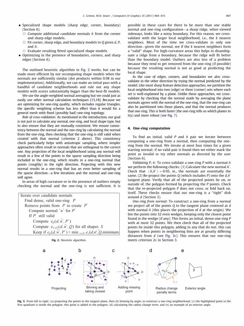
Optimizing in the presence of boundaries, corners, and sharpedges (Section 6).

The outlined heuristic algorithm in Fig. 2 works, but can bemade more efficient by not recomputing shape models when thenormals are sufficiently similar (dot products within 0.98 in ourimplementation). Additionally, we can make an initial pass with ahandful of candidate neighborhoods and rule out any shapemodels with scores substantially bigger than the best-fit models.

We use the angle-weighted normal averaging but we could just aseasily use other normal calculation techniques [15,18]. Because weare optimizing for one-ring quality, which includes regular triangles,the specific weighting scheme has less effect than it would for ageneral mesh with fixed (possibly bad) one-ring topology.

Role of cross-validation: As mentioned in the introduction, our goalis not just to calculate any normal, one-ring, and local shape type, butto also ensure that they are mutually consistent. We ensure consis-tency between the normal and the one-ring by calculating the normalfrom the one-ring, then checking that the one-ring is still valid whencreated with that normal (criterion 2 above). This consistencycheck particularly helps with anisotropic sampling, where simplerapproaches often result in normals that are orthogonal to the correctone. Any projection of the local neighborhood using any normal willresult in a few of the points in the sparse sampling direction beingincluded in the one-ring, which results in a one-ring normal thatpoints (roughly) in the right direction. Projecting with this newnormal results in a one-ring that has an even better sampling ofthe sparse direction—a few iterations and the normal and one-ringwill agree.

In areas of high curvature or in the presence of outliers simplychecking the normal and the one-ring is not sufficient. It is

Fig. 2. Heuristic algorithm.

d

n

Projecting

qi pid

Binning andtaking closest

Addingp

rom left to right: (a) projecting the points to the tangent plane, then (b) binnin

drant is inside the polygon; this point is added to the polygon; (d) calculating

possible in these cases for there to be more than one stablenormal and one-ring configuration—a sharp ridge, when viewedsideways, looks like a noisy boundary. For this reason, we cross-validate with the larger local neighborhood, i.e., the k nearestneighbors. Most of the time we cross-validate in only onedirection—given the normal, see if the k nearest neighbors forma ‘‘valid’’ shape. For high-curvature areas this helps to disambig-uate a ridge from a boundary, because the ridge will fit betterthan the boundary model. Outliers are also less of a problembecause they tend to get removed from the one-ring (if possible)because the resulting normal is not as good at predicting thelocal shape.

In the case of edges, corners, and boundaries we also cross-validate in the other direction by trying the normal predicted by themodel. Like most sharp feature detection approaches, we partition thelocal neighborhood into two (edge) or three (corner) sets where eachset is well-explained by a plane. Unlike these approaches, we cross-validate by checking that the normal made by averaging the planenormals agrees with the normal of the one-ring, that the one-ring canalso be partitioned into those planes, and that the normal producesthat one-ring. This is both faster (the one-ring tells us which planes totry) and more robust (see Fig. 7).

4. One-ring computation

To find an initial, valid P and n pair we iterate betweencomputing a one-ring from a normal, then computing the one-ring from the normal. We iterate at most four times for a givenstarting normal; if no valid pair is found then we either mark thepoint as invalid or try other normals as directed by the user(Section 6).

Validating P, n: To cross-validate a one-ring P with a normal n

we perform the following checks: (1) Calculate the new normal n0.

Check that /n,n0S40:95, ie., the normals are essentially the

same. (2) Re-project the points Q (which includes P) onto the d,n0

tangent plane. Verify that all of the projected points lie on, oroutside of, the polygon formed by projecting the P points. Checkthat the re-projected polygon P does not cross, or fold back on,itself. These checks ensure that our one-ring is a ‘‘tight’’ diskaround d (Section 3).

One-ring from normal: To construct a one-ring from a normalwe project all of the points Q to the tangent plane centered at d

with normal n (this places the projection of d at the origin). Webin the points into 32 even wedges, keeping only the closest pointfound in the wedge (if any). This forms an initial, dense one-ring P

with at most 32 points. We then check that all of the projectedpoints lie inside this polygon, adding in any that do not; this canhappen when points in neighboring bins are at greatly differingdistances from d (see Fig. 3c). This ensures that our one-ringmeets criterion 2c in Section 3.

missingoint

ri-1

ri-1

r

Radius changepenalty terms

Exterior angle

αi+1αi-1 β

g by angle, to construct a one-ring neighborhood; (c) the highlighted point in the

the radius change term; and (e) an example of an exterior angle.

C. Grimm, W.D. Smart / Computers & Graphics 35 (2011) 904–915908

Normal from one-ring: We use the standard angle-weightednormal averaging [18] with one exception; we use a decreasingweight for angles bigger than 25% of the total. These representgaps in the data.

Initial normals: We compute the singular value decompositionof the k�3 matrix Qj�d and use all three vectors as initial,candidate normals. Other candidate normals may be added if wedetect edges, corners, or boundaries (Section 6).

4.1. One-ring evaluation

The ideal one-ring neighborhood P is one that surrounds d,with d roughly in the center and the points in P evenly distributedaround d. We evaluate the quality of P not in 3D, but using the 2Dpolygon created by projecting the points P onto the tangent plane.Our metric epðd,n,PÞ is the average of three terms: even anglespacing, minimal change in radius length, and how centered thepoint d is. We then add to epðd,n,PÞ an additional term whichpenalizes concave polygons (see Fig. 3e).

Let n be the number of points in the projected polygon P, and pi

be the projection of the ith point of P. The angle term ea(i) is thedifference, squared, of the angle ai from the average, divided bythe average. The radius change term er(i) is the differencebetween the radius at pi and the average of the previous andnext radii (weighted by angle) and scaled by the overall radius.The centered term ec is the difference between the polygon’scentroid and the origin, divided by the maximum polygon radiusR. The convexity term ex is the exterior angle (divided by p) forany convex boundary point. The first three terms are normalizedso they can be combined; the convexity term grows as the one-ring becomes concave:

eaðiÞ ¼ai�

1

n

Pjaj

1

n

Pjaj

0B@

1CA

2

ð1Þ

erðiÞ ¼

ri�1

2

ai�1

ai�1þaiþ1ri�1þ

aiþ1

ai�1þaiþ1riþ1

� �� �riþri�1þriþ1

0BB@

1CCA

2

ð2Þ

ecðPÞ ¼

1

n

Pipi

��������

Rð3Þ

Flat

d

Tangent plan

dLine

Ridge

Plane 1Edge

n n

n

Plane 2

Pl

Plane 1

x

y

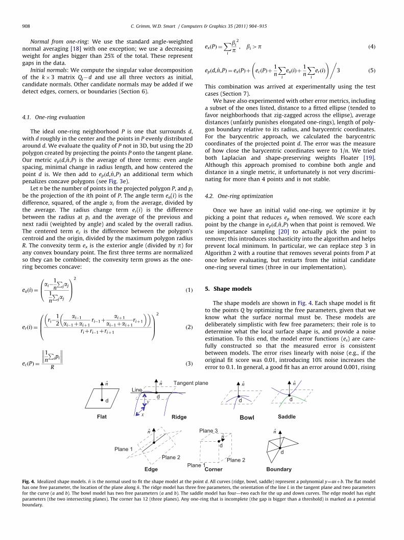
Fig. 4. Idealized shape models. n is the normal used to fit the shape model at the point

has one free parameter, the location of the plane along n . The ridge model has three fre

for the curve (a and b). The bowl model has two free parameters (a and b). The saddle

parameters (the two intersecting planes). The corner has 12 (three planes). Any one-ri

boundary.

exðPÞ ¼X

i

bi

p

2

, bi4p ð4Þ

epðd,n,PÞ ¼ exðPÞþ ecðPÞþ1

n

Xi

eaðiÞþ1

n

Xi

erðiÞ

!,3 ð5Þ

This combination was arrived at experimentally using the testcases (Section 7).

We have also experimented with other error metrics, includinga subset of the ones listed, distance to a fitted ellipse (tended tofavor neighborhoods that zig-zagged across the ellipse), averagedistances (unfairly punishes elongated one-rings), length of poly-gon boundary relative to its radius, and barycentric coordinates.For the barycentric approach, we calculated the barycentriccoordinates of the projected point d. The error was the measureof how close the barycentric coordinates were to 1/n. We triedboth Laplacian and shape-preserving weights Floater [19].Although this approach promised to combine both angle anddistance in a single metric, it unfortunately is not very discrimi-nating for more than 4 points and is not stable.

4.2. One-ring optimization

Once we have an initial valid one-ring, we optimize it bypicking a point that reduces ep when removed. We score eachpoint by the change in epðd,n,PÞ when that point is removed. Weuse importance sampling [20] to actually pick the point toremove; this introduces stochasticity into the algorithm and helpsprevent local minimum. In particular, we can replace step 3 inAlgorithm 2 with a routine that removes several points from P atonce before evaluating, but restarts from the initial candidateone-ring several times (three in our implementation).

5. Shape models

The shape models are shown in Fig. 4. Each shape model is fitto the points Q by optimizing the free parameters, given that weknow what the surface normal must be. These models aredeliberately simplistic with few free parameters; their role is todetermine what the local surface shape is, and provide a noiseestimation. To this end, the model error functions (es) are care-fully constructed so that the measured error is consistentbetween models. The error rises linearly with noise (e.g., if theoriginal fit score was 0.01, introducing 10% noise increases theerror to 0.1. In general, a good fit has an error around 0.001, rising

e

d d

Saddle

d

Corner

d

Boundary

n n

nn

Plane 2

ane 3

Bowl

d. All curves (ridge, bowl, saddle) represent a polynomial y¼axþb. The flat model

e parameters, the orientation of the line L in the tangent plane and two parameters

model has four—two each for the up and down curves. The edge model has eight

ng that is incomplete (the gap is bigger than a threshold) is marked as a potential

C. Grimm, W.D. Smart / Computers & Graphics 35 (2011) 904–915 909

to 0.2 for a tolerable fit. Errors bigger than that indicate problemsor outliers.

The free parameters are chosen so that the distribution of thepoints has little, or no, effect, provided there are enough points torecognize the shape (i.e., for a ridge there must be points bothalong the ridge and on either side). Because the shapes aresimplistic they tend not to hold for large regions; for that reasonwe use a fall-off weight when solving for the parameters. Thisweight is

la ¼1

k

Xi

Jqi�dJ ð6Þ

wi ¼max 1,1:1�Jqi�dJ�la

maxiJqi�dJ�la

� �ð7Þ

We include the point d when solving for the parameters.A point Qi is considered to be on the tangent plane through d

with normal n if it is projected distance is less than 0.1 of theaverage distance:

1

10k

Xi

JQi�dJ ð8Þ

Flat model: For the flat model we know the surface normal; allthat is left to find is where the tangent plane is located along n

(one degree of freedom). We find this location using a weightedleast-squares solve (Eq. (7)). The error es is the residual error ofthe solve.

Bowl model: The bowl model assumes that the surface liesentirely on one side of the tangent plane passing through d withnormal n, and that points further from d are further below theplane (this ensures that a flat region is not marked as a bowl). Weassume the curving can be modeled by a simple polynomial, y¼a

x2þb, where x is the distance in the tangent plane from d and y is

the distance below the tangent plane. We solve for a,b using aweighted least-squares solve. The reason we include b is to allowthe tangent plane to slide up or down, accounting for noise in thenormal direction at d.

We measure how much the bowl curves down by calculatingthe angle a between the starting point of the polynomial (x¼0)and the ending point x¼maxiJqi�dJ. Angles less than p=16indicate a plane, not a bowl. For angles between p=16 and p=8we introduce a penalty term 0:1ðp=8�aÞ=ðp=16�p=8Þ. This pen-alty is added to the residual fit error to give es.

Ridge model: The difference between the ridge model and thebowl one is that the surface is flush with the tangent plane in onedirection. Given the direction ~t in which the surface is flush, wecalculate a fall-off polynomial as in the bowl model, except weuse the distance to the line dþ~t for x.

We try three different~t directions, taking the one with the bestfit value. (1) Take all of the points that lie on, or near, the tangentplane and fit a line to them; project this line onto the tangentplane. (2 and 3) Calculate a sharp edge model (Section 6).Intersect each of the two resulting planes with the tangent plane.

Saddle model: A saddle is formed by radially alternatingupward curving areas with downward curving ones, i.e., thereare points both above and below the tangent plane, and thefurther from d the point Qi is, the further from the tangent plane itis. To measure the curving, we divide the points into two groups(above and below), putting points that are close to the tangentplane into both groups. We then fit a bowl model to each group.The es term is the average of the two bowl models.

To prevent a noisy local neighborhood from looking like asaddle, we add an additional penalty term to ensure that, in anygiven radial direction, the points all curve up (or down). We binthe points by angle, then count the number of bins that have

points that belong to both the up and down group. We use 4p=k

bins. The penalty term is 0.1 times the number of bad bins.Feature size: For the curved models we use the angle a to

provide an absolute measure of the local feature size. For flatmodels we use the angle a of the best-fit smooth model.

6. Edge, corner, boundary models

If there are sharp edges or corners in the data than we canexplicitly fit a model to them, which results in better normalestimation. The boundary model assumes that the one-ring isincomplete and is used to flag boundary points in the data set. It issafe to include these models even if these features are not presentin the data set; however, it increases the computation cost, whichis why they are optional.

An edge is formed when two planes with sufficiently differentorientations meet. Similarly, a corner is formed when three planesmeet. To determine if we have an edge (or corner) we need to firstfind those two (or three) planes. The observation we use is thatthe triangle wedges of the one-ring (formed by d, Pi, Piþ1) are agood approximation to the planes. We therefore look at all pairs(triplets) of wedges with normals that are sufficiently different(angle difference greater that p=3 for edges, p=4 for corners). Ifthere are no pairs (triplets) then there is no edge (or corner).

Normal calculation: To calculate the normal, we assign eachpoint in Q to one of the candidate planes, assigning it to bothplanes if it is close enough (Eq. (8)). We then fit planes, as in theflat model. To ensure the normals are oriented correctly, they areflipped if they do not point in the same direction as the candidateplanes. The normal is the average of the two (three) planenormals. We only keep normals that pass the validity check inSection 4.

If we find a valid edge or corner model we add that normal tothe list of candidate normals. We cross-validate edge and cornermodels slightly differently. We use the normal found by thecandidate planes and only try one-rings which are valid whenprojected by that normal. We additionally check that, whenwalking around the one-ring, the triangle wedges split into twoconsecutive groups (three for corner) where the normals areapproximately that of the fitted planes.

Edge model: The edge model is a combination of how well theplanes fit (flat model ef ðd,n,Q Þ), the angle a between the planes,whether or not the points lie below the tangent plane (h), andhow close d is to each plane. Let Q1 be the group of pointsassigned to plane one, and similarly for Q2. Let d1 be the distancefrom d to plane one, divided by the average size of the neighbor-hood ðð1=kÞ

PiJqi�dJÞ, and similarly for d2:

h¼X

max 0,li

1

k

PiJqi�dJ

�0:1 ð9Þ

esðd,n,Q Þ ¼ 0:25jQ1jef ðd,n1 ,Q1ÞþjQ2jef ðd,n2 ,Q2Þ

jQ1jþjQ2jð10Þ

þ0:75a�p

2p2

0B@

1CA

2

þd1þd2

2þh

0B@

1CA ð11Þ

where jQ j is the number of points in the set Q. li is the signeddistance of qi to the tangent plane.

Corner model: The corner model is identical to the edge model,except we place the points in three groups, sum over three planes,and compare the normals pair-wise.

Boundary model: Unlike the other shape models, there is nonatural, simple shape for boundaries because they arise when the

C. Grimm, W.D. Smart / Computers & Graphics 35 (2011) 904–915910

sampling process is incomplete, leaving a gap in the data. There-fore, the ‘‘correct’’ shape could be any one of the smooth models,with a piece missing. We use the flat model score for theboundary model score and additionally mark all smooth modelsas being boundaries if they satisfy either of the following:

�

The point (0,0) is not in the projected polygon, i.e., the one-ringis less than half a circle. � Any wedge of the polygon is bigger than 0:8p.

Note that sharp edges and corners can also masquerade asboundaries with noise. If the best smooth shape model is flaggedas being a boundary then the point is marked as a boundary. If thebest shape model is an edge or corner one we check forsufficiently different planes; if the planes are close to at wereturn a boundary. Otherwise, we return the best shape modelas usual.

6.1. Modifications to heuristic algorithm

The regular algorithm uses just three initial, orthogonalvectors. If, after trying these three vectors, all of the smoothmodels are marked as boundaries we do a more exhaustive searchto see if there is a projection direction that results in no gaps. Wetry 12 normal directions, evenly distributed on the sphere; if anyof these pass the no boundary test (items listed above) we add itas a candidate normal in the outer loop.

If we get a boundary model, or the best model score is greaterthan 0.1 we try both adjusting the neighborhood size down(minimum size 6) and up (maximum size 50) in increments of25% of the current size. Shrinking the neighborhood is helpfulwhere the surface passes close to another piece of surface, andgrowing the neighborhood helps with bridging sampling gaps.Provided the inter-surface distance is greater than the intra-sample distance, the shape model that comes from only onesurface will have a better score than one that has samples fromboth surfaces.

7. Evaluation

We evaluated the algorithm in three ways: (1) known surfaces,(2) real data, and (3) comparison to exhaustive search.

Grid ContoHexagonal

Flat Ridge Bowl

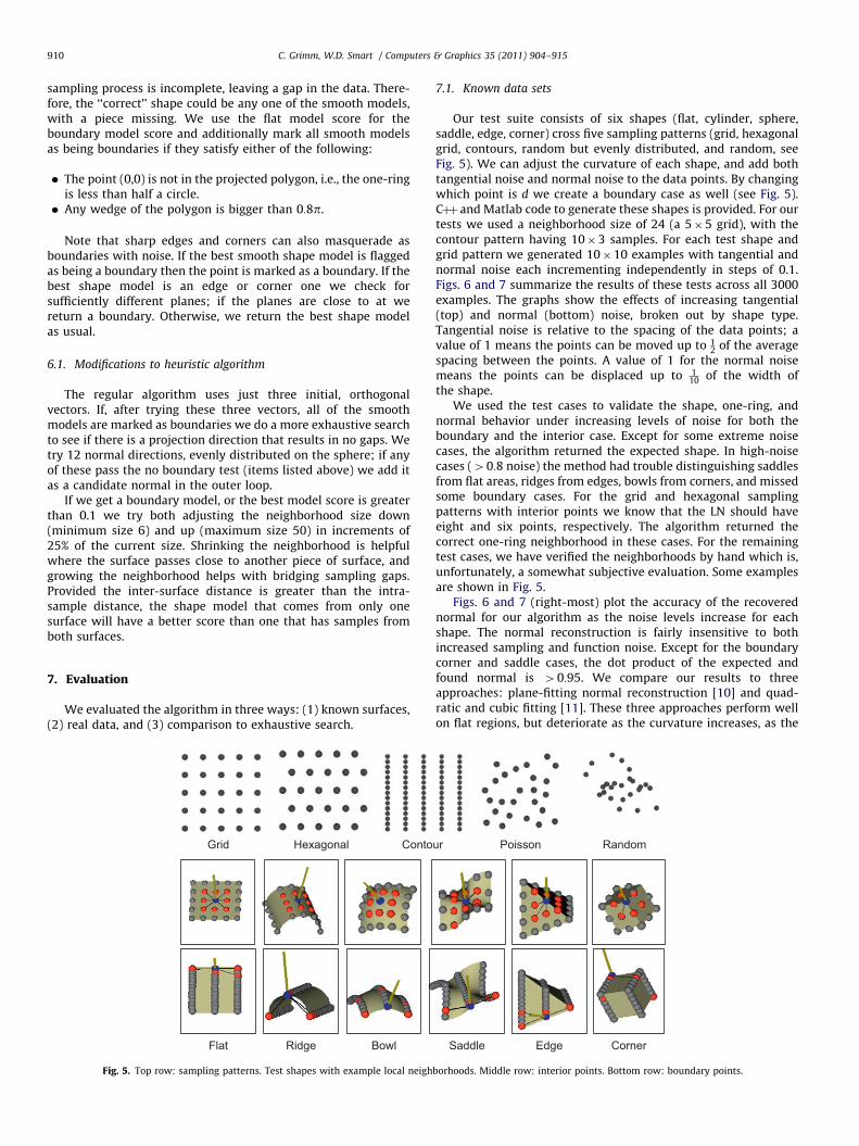
Fig. 5. Top row: sampling patterns. Test shapes with example local neigh

7.1. Known data sets

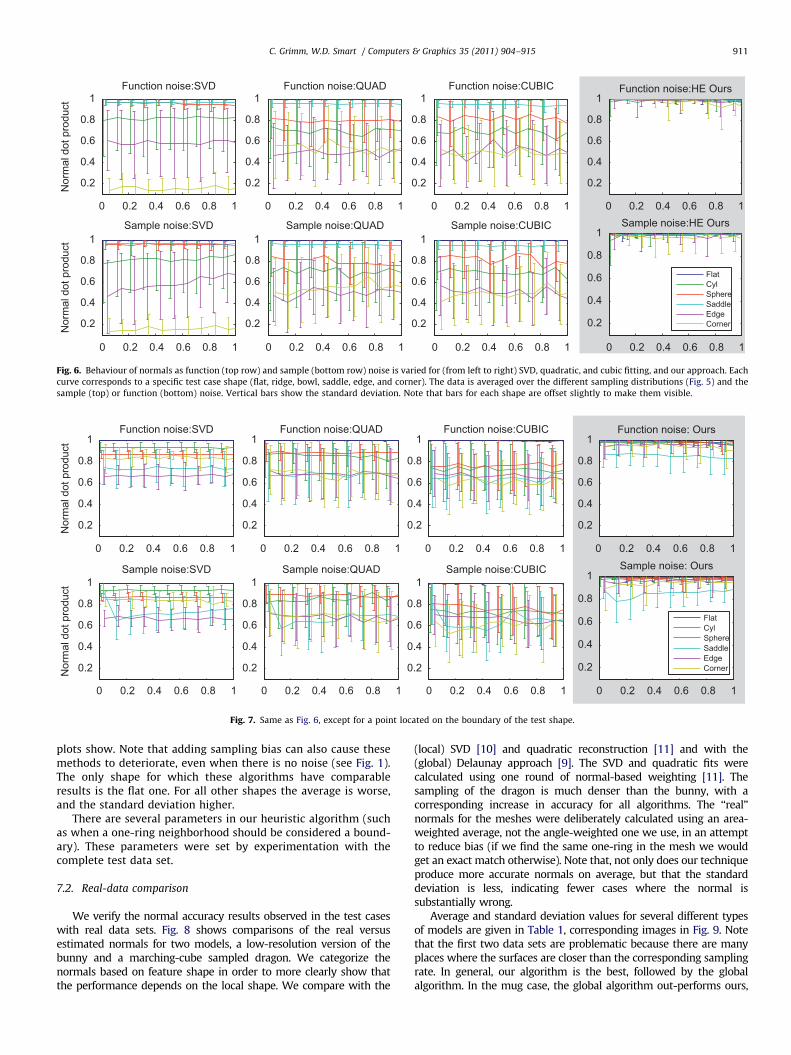
Our test suite consists of six shapes (flat, cylinder, sphere,saddle, edge, corner) cross five sampling patterns (grid, hexagonalgrid, contours, random but evenly distributed, and random, seeFig. 5). We can adjust the curvature of each shape, and add bothtangential noise and normal noise to the data points. By changingwhich point is d we create a boundary case as well (see Fig. 5).Cþþand Matlab code to generate these shapes is provided. For ourtests we used a neighborhood size of 24 (a 5�5 grid), with thecontour pattern having 10�3 samples. For each test shape andgrid pattern we generated 10�10 examples with tangential andnormal noise each incrementing independently in steps of 0.1.Figs. 6 and 7 summarize the results of these tests across all 3000examples. The graphs show the effects of increasing tangential(top) and normal (bottom) noise, broken out by shape type.Tangential noise is relative to the spacing of the data points; avalue of 1 means the points can be moved up to 1

2 of the averagespacing between the points. A value of 1 for the normal noisemeans the points can be displaced up to 1

10 of the width ofthe shape.

We used the test cases to validate the shape, one-ring, andnormal behavior under increasing levels of noise for both theboundary and the interior case. Except for some extreme noisecases, the algorithm returned the expected shape. In high-noisecases (40:8 noise) the method had trouble distinguishing saddlesfrom flat areas, ridges from edges, bowls from corners, and missedsome boundary cases. For the grid and hexagonal samplingpatterns with interior points we know that the LN should haveeight and six points, respectively. The algorithm returned thecorrect one-ring neighborhood in these cases. For the remainingtest cases, we have verified the neighborhoods by hand which is,unfortunately, a somewhat subjective evaluation. Some examplesare shown in Fig. 5.

Figs. 6 and 7 (right-most) plot the accuracy of the recoverednormal for our algorithm as the noise levels increase for eachshape. The normal reconstruction is fairly insensitive to bothincreased sampling and function noise. Except for the boundarycorner and saddle cases, the dot product of the expected andfound normal is 40:95. We compare our results to threeapproaches: plane-fitting normal reconstruction [10] and quad-ratic and cubic fitting [11]. These three approaches perform wellon flat regions, but deteriorate as the curvature increases, as the

Poissonur Random

Saddle Edge Corner

borhoods. Middle row: interior points. Bottom row: boundary points.

0 0.2 0.4 0.6 0.8 1

0.2

0.4

0.6

0.8

1Function noise:SVD

Nor

mal

dot

pro

duct

0 0.2 0.4 0.6 0.8 1

0.2

0.4

0.6

0.8

1Function noise:QUAD

0 0.2 0.4 0.6 0.8 1

0.2

0.4

0.6

0.8

1Function noise:CUBIC

0 0.2 0.4 0.6 0.8 1

0.2

0.4

0.6

0.8

1Function noise:HE Ours

0 0.2 0.4 0.6 0.8 1

0.2

0.4

0.6

0.8

1Sample noise:SVD

Nor

mal

dot

pro

duct

0 0.2 0.4 0.6 0.8 1

0.2

0.4

0.6

0.8

1Sample noise:QUAD

0 0.2 0.4 0.6 0.8 1

0.2

0.4

0.6

0.8

1Sample noise:CUBIC

0 0.2 0.4 0.6 0.8 1

0.2

0.4

0.6

0.8

1Sample noise:HE Ours

FlatCylSphereSaddleEdgeCorner

Fig. 6. Behaviour of normals as function (top row) and sample (bottom row) noise is varied for (from left to right) SVD, quadratic, and cubic fitting, and our approach. Each

curve corresponds to a specific test case shape (flat, ridge, bowl, saddle, edge, and corner). The data is averaged over the different sampling distributions (Fig. 5) and the

sample (top) or function (bottom) noise. Vertical bars show the standard deviation. Note that bars for each shape are offset slightly to make them visible.

0 0.2 0.4 0.6 0.8 1

0.2

0.4

0.6

0.8

1Function noise:SVD

Nor

mal

dot

pro

duct

0 0.2 0.4 0.6 0.8 1

0.2

0.4

0.6

0.8

1Function noise:QUAD

0 0.2 0.4 0.6 0.8 1

0.2

0.4

0.6

0.8

1Function noise:CUBIC

0 0.2 0.4 0.6 0.8 1

0.2

0.4

0.6

0.8

1Function noise: Ours

0 0.2 0.4 0.6 0.8 1

0.2

0.4

0.6

0.8

1Sample noise:SVD

Nor

mal

dot

pro

duct

0 0.2 0.4 0.6 0.8 1

0.2

0.4

0.6

0.8

1Sample noise:QUAD

0 0.2 0.4 0.6 0.8 1

0.2

0.4

0.6

0.8

1Sample noise:CUBIC

0 0.2 0.4 0.6 0.8 1

0.2

0.4

0.6

0.8

1Sample noise: Ours

FlatCylSphereSaddleEdgeCorner

Fig. 7. Same as Fig. 6, except for a point located on the boundary of the test shape.

C. Grimm, W.D. Smart / Computers & Graphics 35 (2011) 904–915 911

plots show. Note that adding sampling bias can also cause thesemethods to deteriorate, even when there is no noise (see Fig. 1).The only shape for which these algorithms have comparableresults is the flat one. For all other shapes the average is worse,and the standard deviation higher.

There are several parameters in our heuristic algorithm (suchas when a one-ring neighborhood should be considered a bound-ary). These parameters were set by experimentation with thecomplete test data set.

7.2. Real-data comparison

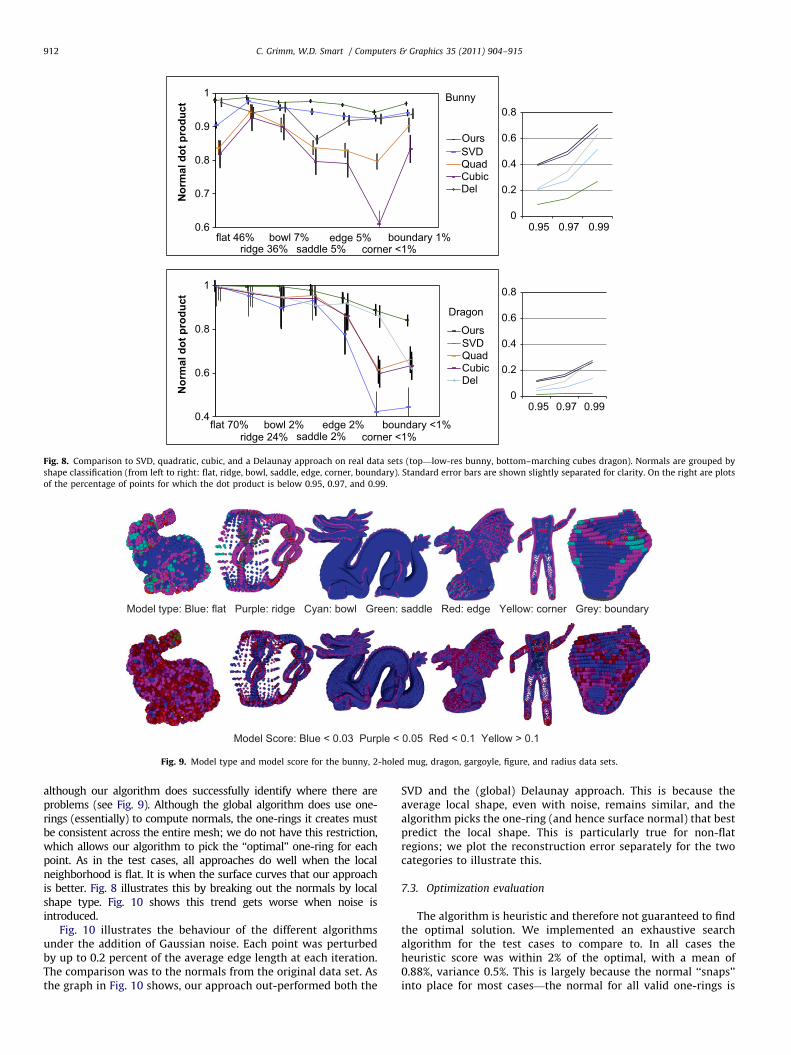
We verify the normal accuracy results observed in the test caseswith real data sets. Fig. 8 shows comparisons of the real versusestimated normals for two models, a low-resolution version of thebunny and a marching-cube sampled dragon. We categorize thenormals based on feature shape in order to more clearly show thatthe performance depends on the local shape. We compare with the

(local) SVD [10] and quadratic reconstruction [11] and with the(global) Delaunay approach [9]. The SVD and quadratic fits werecalculated using one round of normal-based weighting [11]. Thesampling of the dragon is much denser than the bunny, with acorresponding increase in accuracy for all algorithms. The ‘‘real’’normals for the meshes were deliberately calculated using an area-weighted average, not the angle-weighted one we use, in an attemptto reduce bias (if we find the same one-ring in the mesh we wouldget an exact match otherwise). Note that, not only does our techniqueproduce more accurate normals on average, but that the standarddeviation is less, indicating fewer cases where the normal issubstantially wrong.

Average and standard deviation values for several different typesof models are given in Table 1, corresponding images in Fig. 9. Notethat the first two data sets are problematic because there are manyplaces where the surfaces are closer than the corresponding samplingrate. In general, our algorithm is the best, followed by the globalalgorithm. In the mug case, the global algorithm out-performs ours,

0.4

0.6

0.8

1

Nor

mal

dot

pro

duct

SVDQuadCubicDel

0.6

0.7

0.8

0.9

1

Nor

mal

dot

pro

duct

SVDQuadCubicDel

Bunny

Dragon

0

0.2

0.4

0.6

0.8

0.95 0.97 0.99

0

0.2

0.4

0.6

0.8

0.95 0.97 0.99

Ours

Ours

flat 70%ridge 24% saddle 2% corner <1%

ridge 36% saddle 5% corner <1%

bowl 2% edge 2% boundary <1%

flat 46% bowl 7% edge 5% boundary 1%

Fig. 8. Comparison to SVD, quadratic, cubic, and a Delaunay approach on real data sets (top—low-res bunny, bottom–marching cubes dragon). Normals are grouped by

shape classification (from left to right: flat, ridge, bowl, saddle, edge, corner, boundary). Standard error bars are shown slightly separated for clarity. On the right are plots

of the percentage of points for which the dot product is below 0.95, 0.97, and 0.99.

Model type: Blue: flat Purple: ridge Cyan: bowl Green: saddle Red: edge Yellow: corner Grey: boundary

Model Score: Blue < 0.03 Purple < 0.05 Red < 0.1 Yellow > 0.1

Fig. 9. Model type and model score for the bunny, 2-holed mug, dragon, gargoyle, figure, and radius data sets.

C. Grimm, W.D. Smart / Computers & Graphics 35 (2011) 904–915912

although our algorithm does successfully identify where there areproblems (see Fig. 9). Although the global algorithm does use one-rings (essentially) to compute normals, the one-rings it creates mustbe consistent across the entire mesh; we do not have this restriction,which allows our algorithm to pick the ‘‘optimal’’ one-ring for eachpoint. As in the test cases, all approaches do well when the localneighborhood is flat. It is when the surface curves that our approachis better. Fig. 8 illustrates this by breaking out the normals by localshape type. Fig. 10 shows this trend gets worse when noise isintroduced.

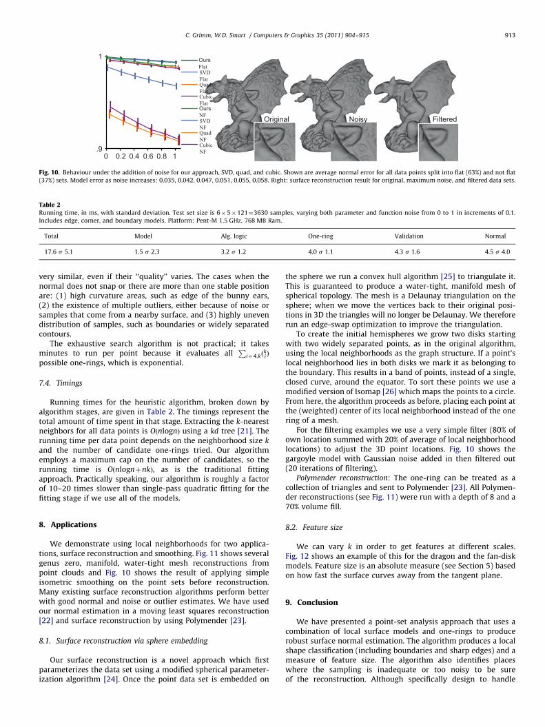
Fig. 10 illustrates the behaviour of the different algorithmsunder the addition of Gaussian noise. Each point was perturbedby up to 0.2 percent of the average edge length at each iteration.The comparison was to the normals from the original data set. Asthe graph in Fig. 10 shows, our approach out-performed both the

SVD and the (global) Delaunay approach. This is because theaverage local shape, even with noise, remains similar, and thealgorithm picks the one-ring (and hence surface normal) that bestpredict the local shape. This is particularly true for non-flatregions; we plot the reconstruction error separately for the twocategories to illustrate this.

7.3. Optimization evaluation

The algorithm is heuristic and therefore not guaranteed to findthe optimal solution. We implemented an exhaustive searchalgorithm for the test cases to compare to. In all cases theheuristic score was within 2% of the optimal, with a mean of0.88%, variance 0.5%. This is largely because the normal ‘‘snaps’’into place for most cases—the normal for all valid one-rings is

FilteredNoisyOriginal

0

SVDFlatQuadFlatCubicFlat

SVDNFQuadNFCubicNF

1

.9

OursFlat

OursNF

0.2 0.4 0.6 0.8 1

Fig. 10. Behaviour under the addition of noise for our approach, SVD, quad, and cubic. Shown are average normal error for all data points split into flat (63%) and not flat

(37%) sets. Model error as noise increases: 0.035, 0.042, 0.047, 0.051, 0.055, 0.058. Right: surface reconstruction result for original, maximum noise, and filtered data sets.

Table 2Running time, in ms, with standard deviation. Test set size is 6�5�121¼3630 samples, varying both parameter and function noise from 0 to 1 in increments of 0.1.

Includes edge, corner, and boundary models. Platform: Pent-M 1.5 GHz, 768 MB Ram.

Total Model Alg. logic One-ring Validation Normal

17.6 s 5.1 1.5 s 2.3 3.2 s 1.2 4.0 s 1.1 4.3 s 1.6 4.5 s 4.0

C. Grimm, W.D. Smart / Computers & Graphics 35 (2011) 904–915 913

very similar, even if their ‘‘quality’’ varies. The cases when thenormal does not snap or there are more than one stable positionare: (1) high curvature areas, such as edge of the bunny ears,(2) the existence of multiple outliers, either because of noise orsamples that come from a nearby surface, and (3) highly unevendistribution of samples, such as boundaries or widely separatedcontours.

The exhaustive search algorithm is not practical; it takesminutes to run per point because it evaluates all

PiA4,kð

kiÞ

possible one-rings, which is exponential.

7.4. Timings

Running times for the heuristic algorithm, broken down byalgorithm stages, are given in Table 2. The timings represent thetotal amount of time spent in that stage. Extracting the k-nearestneighbors for all data points is OðnlognÞ using a kd tree [21]. Therunning time per data point depends on the neighborhood size k

and the number of candidate one-rings tried. Our algorithmemploys a maximum cap on the number of candidates, so therunning time is OðnlognþnkÞ, as is the traditional fittingapproach. Practically speaking, our algorithm is roughly a factorof 10–20 times slower than single-pass quadratic fitting for thefitting stage if we use all of the models.

8. Applications

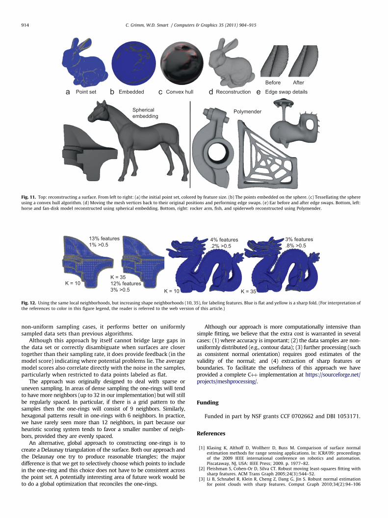
We demonstrate using local neighborhoods for two applica-tions, surface reconstruction and smoothing. Fig. 11 shows severalgenus zero, manifold, water-tight mesh reconstructions frompoint clouds and Fig. 10 shows the result of applying simpleisometric smoothing on the point sets before reconstruction.Many existing surface reconstruction algorithms perform betterwith good normal and noise or outlier estimates. We have usedour normal estimation in a moving least squares reconstruction[22] and surface reconstruction by using Polymender [23].

8.1. Surface reconstruction via sphere embedding

Our surface reconstruction is a novel approach which firstparameterizes the data set using a modified spherical parameter-ization algorithm [24]. Once the point data set is embedded on

the sphere we run a convex hull algorithm [25] to triangulate it.This is guaranteed to produce a water-tight, manifold mesh ofspherical topology. The mesh is a Delaunay triangulation on thesphere; when we move the vertices back to their original posi-tions in 3D the triangles will no longer be Delaunay. We thereforerun an edge-swap optimization to improve the triangulation.

To create the initial hemispheres we grow two disks startingwith two widely separated points, as in the original algorithm,using the local neighborhoods as the graph structure. If a point’slocal neighborhood lies in both disks we mark it as belonging tothe boundary. This results in a band of points, instead of a single,closed curve, around the equator. To sort these points we use amodified version of Isomap [26] which maps the points to a circle.From here, the algorithm proceeds as before, placing each point atthe (weighted) center of its local neighborhood instead of the onering of a mesh.

For the filtering examples we use a very simple filter (80% ofown location summed with 20% of average of local neighborhoodlocations) to adjust the 3D point locations. Fig. 10 shows thegargoyle model with Gaussian noise added in then filtered out(20 iterations of filtering).

Polymender reconstruction: The one-ring can be treated as acollection of triangles and sent to Polymender [23]. All Polymen-der reconstructions (see Fig. 11) were run with a depth of 8 and a70% volume fill.

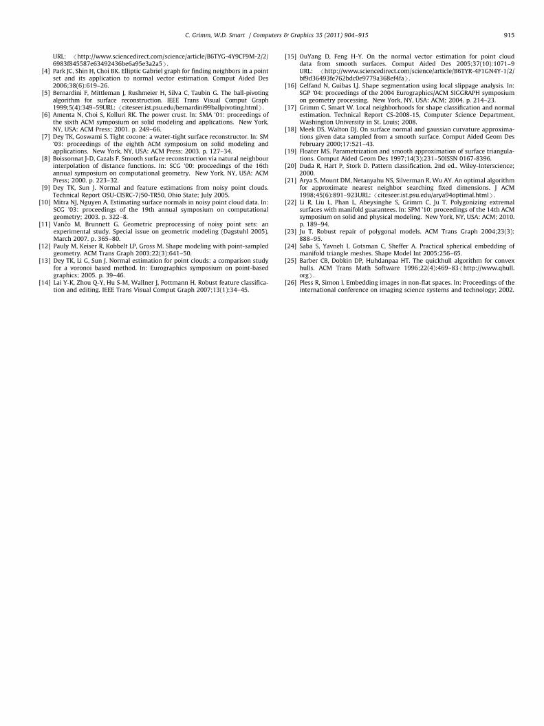
8.2. Feature size

We can vary k in order to get features at different scales.Fig. 12 shows an example of this for the dragon and the fan-diskmodels. Feature size is an absolute measure (see Section 5) basedon how fast the surface curves away from the tangent plane.

9. Conclusion

We have presented a point-set analysis approach that uses acombination of local surface models and one-rings to producerobust surface normal estimation. The algorithm produces a localshape classification (including boundaries and sharp edges) and ameasure of feature size. The algorithm also identifies placeswhere the sampling is inadequate or too noisy to be sureof the reconstruction. Although specifically design to handle

13% features1% >0.5

K = 10K = 3512% features3% >0.5 K = 35K = 10

4% features.2% >0.5

3% features.8% >0.5

Fig. 12. Using the same local neighborhoods, but increasing shape neighborhoods (10, 35), for labeling features. Blue is flat and yellow is a sharp fold. (For interpretation of

the references to color in this figure legend, the reader is referred to the web version of this article.)

Point set Convex hull

Before

Edge swap details

PolymenderSphericalembedding

Embedded Reconstruction

After

Fig. 11. Top: reconstructing a surface. From left to right: (a) the initial point set, colored by feature size. (b) The points embedded on the sphere. (c) Tessellating the sphere

using a convex hull algorithm. (d) Moving the mesh vertices back to their original positions and performing edge swaps. (e) Ear before and after edge swaps. Bottom, left:

horse and fan-disk model reconstructed using spherical embedding. Bottom, right: rocker arm, fish, and spiderweb reconstructed using Polymender.

C. Grimm, W.D. Smart / Computers & Graphics 35 (2011) 904–915914

non-uniform sampling cases, it performs better on uniformlysampled data sets than previous algorithms.

Although this approach by itself cannot bridge large gaps inthe data set or correctly disambiguate when surfaces are closertogether than their sampling rate, it does provide feedback (in themodel score) indicating where potential problems lie. The averagemodel scores also correlate directly with the noise in the samples,particularly when restricted to data points labeled as flat.

The approach was originally designed to deal with sparse oruneven sampling. In areas of dense sampling the one-rings will tendto have more neighbors (up to 32 in our implementation) but will stillbe regularly spaced. In particular, if there is a grid pattern to thesamples then the one-rings will consist of 9 neighbors. Similarly,hexagonal patterns result in one-rings with 6 neighbors. In practice,we have rarely seen more than 12 neighbors, in part because ourheuristic scoring system tends to favor a smaller number of neigh-bors, provided they are evenly spaced.

An alternative, global approach to constructing one-rings is tocreate a Delaunay triangulation of the surface. Both our approach andthe Delaunay one try to produce reasonable triangles; the majordifference is that we get to selectively choose which points to includein the one-ring and this choice does not have to be consistent acrossthe point set. A potentially interesting area of future work would beto do a global optimization that reconciles the one-rings.

Although our approach is more computationally intensive thansimple fitting, we believe that the extra cost is warranted in severalcases: (1) where accuracy is important; (2) the data samples are non-uniformly distributed (e.g., contour data); (3) further processing (suchas consistent normal orientation) requires good estimates of thevalidity of the normal; and (4) extraction of sharp features orboundaries. To facilitate the usefulness of this approach we haveprovided a complete Cþþ implementation at https://sourceforge.net/projects/meshprocessing/.

Funding

Funded in part by NSF grants CCF 0702662 and DBI 1053171.

References

[1] Klasing K, Althoff D, Wollherr D, Buss M. Comparison of surface normalestimation methods for range sensing applications. In: ICRA’09: proceedingsof the 2009 IEEE international conference on robotics and automation.Piscataway, NJ, USA: IEEE Press; 2009. p. 1977–82.

[2] Fleishman S, Cohen-Or D, Silva CT. Robust moving least-squares fitting withsharp features. ACM Trans Graph 2005;24(3):544–52.

[3] Li B, Schnabel R, Klein R, Cheng Z, Dang G, Jin S. Robust normal estimationfor point clouds with sharp features. Comput Graph 2010;34(2):94–106

C. Grimm, W.D. Smart / Computers & Graphics 35 (2011) 904–915 915

URL: /http://www.sciencedirect.com/science/article/B6TYG-4Y9CF9M-2/2/6983f845587e63492436be6a95e3a2a5S.

[4] Park JC, Shin H, Choi BK. Elliptic Gabriel graph for finding neighbors in a pointset and its application to normal vector estimation. Comput Aided Des2006;38(6):619–26.

[5] Bernardini F, Mittleman J, Rushmeier H, Silva C, Taubin G. The ball-pivotingalgorithm for surface reconstruction. IEEE Trans Visual Comput Graph1999;5(4):349–59URL: /citeseer.ist.psu.edu/bernardini99ballpivoting.htmlS.

[6] Amenta N, Choi S, Kolluri RK. The power crust. In: SMA ’01: proceedings ofthe sixth ACM symposium on solid modeling and applications. New York,NY, USA: ACM Press; 2001. p. 249–66.

[7] Dey TK, Goswami S. Tight cocone: a water-tight surface reconstructor. In: SM’03: proceedings of the eighth ACM symposium on solid modeling andapplications. New York, NY, USA: ACM Press; 2003. p. 127–34.

[8] Boissonnat J-D, Cazals F. Smooth surface reconstruction via natural neighbourinterpolation of distance functions. In: SCG ’00: proceedings of the 16thannual symposium on computational geometry. New York, NY, USA: ACMPress; 2000. p. 223–32.

[9] Dey TK, Sun J. Normal and feature estimations from noisy point clouds.Technical Report OSU-CISRC-7/50-TR50, Ohio State; July 2005.

[10] Mitra NJ, Nguyen A. Estimating surface normals in noisy point cloud data. In:SCG ’03: proceedings of the 19th annual symposium on computationalgeometry; 2003. p. 322–8.

[11] Vanco M, Brunnett G. Geometric preprocessing of noisy point sets: anexperimental study. Special issue on geometric modeling (Dagstuhl 2005),March 2007. p. 365–80.

[12] Pauly M, Keiser R, Kobbelt LP, Gross M. Shape modeling with point-sampledgeometry. ACM Trans Graph 2003;22(3):641–50.

[13] Dey TK, Li G, Sun J. Normal estimation for point clouds: a comparison studyfor a voronoi based method. In: Eurographics symposium on point-basedgraphics; 2005. p. 39–46.

[14] Lai Y-K, Zhou Q-Y, Hu S-M, Wallner J, Pottmann H. Robust feature classifica-tion and editing. IEEE Trans Visual Comput Graph 2007;13(1):34–45.

[15] OuYang D, Feng H-Y. On the normal vector estimation for point clouddata from smooth surfaces. Comput Aided Des 2005;37(10):1071–9URL: /http://www.sciencedirect.com/science/article/B6TYR-4F1GN4Y-1/2/bf9d36493fe762bdc0e9779a368ef4faS.

[16] Gelfand N, Guibas LJ. Shape segmentation using local slippage analysis. In:SGP ’04: proceedings of the 2004 Eurographics/ACM SIGGRAPH symposiumon geometry processing. New York, NY, USA: ACM; 2004. p. 214–23.

[17] Grimm C, Smart W. Local neighborhoods for shape classification and normalestimation. Technical Report CS-2008-15, Computer Science Department,Washington University in St. Louis; 2008.

[18] Meek DS, Walton DJ. On surface normal and gaussian curvature approxima-tions given data sampled from a smooth surface. Comput Aided Geom DesFebruary 2000;17:521–43.

[19] Floater MS. Parametrization and smooth approximation of surface triangula-tions. Comput Aided Geom Des 1997;14(3):231–50ISSN 0167-8396.

[20] Duda R, Hart P, Stork D. Pattern classification. 2nd ed.. Wiley-Interscience;2000.

[21] Arya S, Mount DM, Netanyahu NS, Silverman R, Wu AY. An optimal algorithmfor approximate nearest neighbor searching fixed dimensions. J ACM1998;45(6):891–923URL: /citeseer.ist.psu.edu/arya94optimal.htmlS.

[22] Li R, Liu L, Phan L, Abeysinghe S, Grimm C, Ju T. Polygonizing extremalsurfaces with manifold guarantees. In: SPM ’10: proceedings of the 14th ACMsymposium on solid and physical modeling. New York, NY, USA: ACM; 2010.p. 189–94.

[23] Ju T. Robust repair of polygonal models. ACM Trans Graph 2004;23(3):888–95.

[24] Saba S, Yavneh I, Gotsman C, Sheffer A. Practical spherical embedding ofmanifold triangle meshes. Shape Model Int 2005:256–65.

[25] Barber CB, Dobkin DP, Huhdanpaa HT. The quickhull algorithm for convexhulls. ACM Trans Math Software 1996;22(4):469–83/http://www.qhull.orgS.

[26] Pless R, Simon I. Embedding images in non-flat spaces. In: Proceedings of theinternational conference on imaging science systems and technology; 2002.