Short-Run and Long-Run Money Demand: Recent Evidence · Short-Run and Long-Run Money Demand: Recent Evidence Bharat R. Kolluri University of Hartford Rao Singamsetti University of

Short-Run and Long-Run Money Demand: Recent Evidence

Bharat R. Kolluri University of Hartford

Rao Singamsetti

University of Hartford

Mahmoud Wahab University of Hartford

The role of money and the demand for money continues to be, in principle, a prominent topic of interest in the conduct of monetary policy in the US economy. An attempt is made in this paper to estimate a money demand function with national income and interest rates assumed to be primary drivers of aggregate demand for money. A test of mean-stationarity of estimated coefficients of the money demand function is conducted to determine whether or not the coefficients exhibit mean-stationarity in levels and in first differences. We present the short-run as well as the long-term elasticity estimates for income and nominal interest rate for the US economy using quarterly time series data going back from the mid fifties to the present. INTRODUCTION

In this paper, we estimate aggregate money demand for the US economy using M1 and M2 monetary aggregates. As is well known, aggregate demand for money in the economy comes from households, businesses, and the government sector. A primary objective of monetary authorities is to anticipate money demand and provide the needed level of money supply that maintains desired levels of output, employment, and price stability. While some view interest rate-targeting as the more important monetary policy target than money demand-targeting, we still view money demand and its stability as an important monetary policy issue due to its direct link with money supply, interest rates, and economic growth. Hence, money demand should play an important role directly or indirectly in the conduct of any monetary policy. A detailed presentation on alternative views of targeting monetary aggregates versus interest rates is available in Duca and VanHoose (2004). A number of researchers have examined aggregate demand for money, its stability, and its determinants, particularly, income and interest rates. Unfortunately, studies have reported different results, and have reached differing conclusions which makes it hard to form a clear consensus of opinions1. This wide variation among results may be attributed in part to the different model-specifications and estimation procedures used. Some of the recent studies have employed newer time-series econometric procedures such as cointegration and error correction to correct some of the serious deficiencies inherent in traditional estimation procedures, and have made significant contributions in presenting more efficient and reliable estimates. However, a major drawback still remains in the existing literature, particularly one that is attributed to a failure to present estimates of the long-run

Journal of Accounting and Finance vol. 12(3) 2012 91

fundamental marginal effects of income and interest rates by presenting their elasticity estimates that are derivable from their estimated short-run counterparts. This is an issue of importance for any discussion of long-term policy implications of the effects of income growth and interest rates on money demand. Examples of publications that have employed cointegration and error correction models of money demand include Bose and Rahman (1996), Tai-Hsin Huang (1999), Drama and Chen (2011) among others. This paper rectifies this shortcoming in the literature by presenting estimates of the long-run elasticity of money demand with respect to income and interest rates. We distinguish long-run from short-run estimated relationships between money demand, income and interest rates employing cointegration and error-correction modeling. However, in contrast to existing studies that utilized similar methodologies, we go one step further by allowing estimated parameters to vary over time when generating predicted values of demand for money in the form of M1 and M2 monetary aggregates2.

The origins of money demand instability can be traced back to enactment of the Depository Institution’s Deregulation and Monetary Control Act of 1980, the explosion that took place in development of new financial products and instruments, technological innovation, and last but not least, burgeoning federal deficits stating in the early 1980s coupled with chronic deficit spending and debt monetization by the Federal Reserve, among others. The Federal Reserve Bank cannot effectively conduct monetary policy without sufficient stability of money demand. In addition, the ability to generate more accurate forecasts of money demand is needed for the conduct of interest rate-targeting by monetary authorities. If the estimated coefficients of the money demand function are sensitive to newly included information, thus varying over time, statistical inference based on a constant coefficients model using full-sample estimates can be misleading. We test whether or not the estimated coefficients vary continuously over time, and if so, we embed the information on their time series properties in generating better money demand estimates. To test for time-variation in the estimated coefficients of the money demand function, we apply the chow test on a rolling basis at multiple breakpoints which are set at eight observation (8 quarters) apart (shorter and longer periods in between break points led to similar results, so that results are not sensitive to the adopted breakpoint frequency, and the evidence is fairly conclusive that the estimated parameters of money demand functions for both M1 and M2 monetary aggregates are time-varying with almost complete certainty. Once confirmed by the rolling chow test of parameter instability both in-sample as well as out-of-sample, we proceed to capture the time series properties of the parameters and exploit their stochastic properties in generating out-of-sample predictions of demand for the two monetary aggregates. METHODOLOGY AND DATA

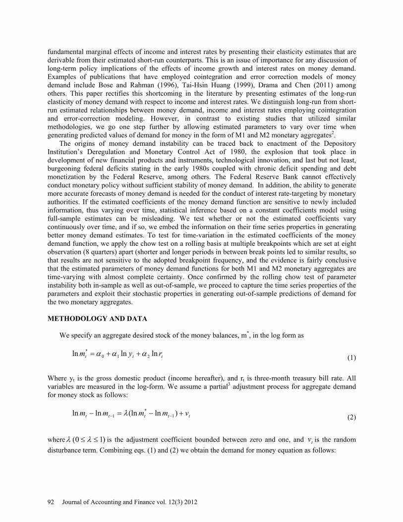
We specify an aggregate desired stock of the money balances, m*, in the log form as

ttt rym lnlnln 210* ααα ++= (1)

Where yt is the gross domestic product (income hereafter), and rt is three-month treasury bill rate. All variables are measured in the log-form. We assume a partial3 adjustment process for aggregate demand for money stock as follows:

ttttt vmmmm +−=− −− )ln(lnlnln 1*

1 λ (2)

where )10( ≤≤ λλ is the adjustment coefficient bounded between zero and one, and tv is the random disturbance term. Combining eqs. (1) and (2) we obtain the demand for money equation as follows:

92 Journal of Accounting and Finance vol. 12(3) 2012

ttttt vmrym +−+++= −1210 ln)1(lnlnln λλαλαλα (3)

This is considered to be the long run reduced-form equilibrium relationship of money demand. In

general, aggregate income facilitates transactions and is, thus, expected to have a significant positive effect on money demand, while the interest rate variable is expected to have a negative impact as it reflects the opportunity cost of holding money. The data used is quarterly monetary aggregates, income and interest rates (90-day T.bill rate) for the period from Q1-1954 to Q4-2008 for the US. All data are in current US dollars. The nominal 90-day T.bill interest rate embeds both the real interest rate and expected inflation components. STATIONARITY AND COINTEGRATION

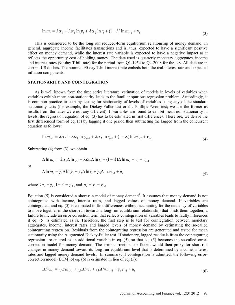
As is well known from the time series literature, estimation of models in levels of variables when variables exhibit mean non-stationarity leads to the familiar spurious regression problem. Accordingly, it is common practice to start by testing for stationarity of levels of variables using any of the standard stationarity tests (for example, the Dickey-Fuller test or the Phillips-Peron test; we use the former as results from the latter were not any different). If variables are found to exhibit mean non-stationarity in levels, the regression equation of eq. (3) has to be estimated in first differences. Therefore, we derive the first differenced form of eq. (3) by lagging it one period then subtracting the lagged from the concurrent equation as follows:

12121101 ln)1(lnlnln −−−−− +−+++= ttttt vmrym λλαλαλα (4)

Subtracting (4) from (3), we obtain

121 ln)1(lnlnln −−+∆−+∆+∆=∆ tttttt vvmrym λλαλα or

ttttt umrym +∆+∆+∆=∆ −1321 lnlnlnln γγγ (5)

where 11 γλα = , 31 γλ =− , and 1−−= ttt vvu Equation (5) is considered a short-run model of money demand4. It assumes that money demand is not cointegrated with income, interest rates, and lagged values of money demand. If variables are cointegrated, and eq. (5) is estimated in first differences without accounting for the tendency of variables to move together in the short-run towards a long-run equilibrium relationship that binds them together, a failure to include an error correction term that reflects cointegration of variables leads to faulty inferences if eq. (5) is estimated as is. Therefore, the first step is to test for cointegration between monetary aggregates, income, interest rates and lagged levels of money demand by estimating the so-called cointegrating regression. Residuals from the cointegrating regression are generated and tested for mean stationarity using the Augmented Dickey-Fuller test. If stationary, lagged residuals from the cointegrating regression are entered as an additional variable in eq. (5), so that eq. (5) becomes the so-called error-correction model for money demand. The error correction coefficient would then proxy for short-run changes in money demand toward its long-run equilibrium level that is determined by income, interest rates and lagged money demand levels. In summary, if cointegration is admitted, the following error-correction model (ECM) of eq. (6) is estimated in lieu of eq. (5):

t1t41t3t2t1t ueγmlnΔγrlnΔγylnΔγmlnΔ ++++= -- (6)


where 1−te represents lagged error correction term corresponding to lagged disequilibrium shocks. The

coefficient of 1−te is expected to be negative and indicates the magnitude of short-run adjustments in money demand toward long run equilibrium cointegration with income and interest rates; essentially, it corrects deviations of money demand from its long-run equilibrium value, and can be regarded as indicative of the speed of adjustment in money demand. The coefficients in eq. (6) for income and interest rates reflect short-term responses of money demand to changes in the exogenous variables, income and interest rates. AN ALTERNATIVE VIEW OF MONEY DEMAND

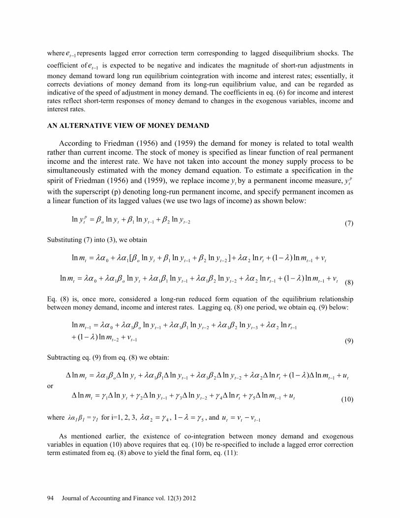
According to Friedman (1956) and (1959) the demand for money is related to total wealth rather than current income. The stock of money is specified as linear function of real permanent income and the interest rate. We have not taken into account the money supply process to be simultaneously estimated with the money demand equation. To estimate a specification in the spirit of Friedman (1956) and (1959), we replace income ty by a permanent income measure, p

ty with the superscript (p) denoting long-run permanent income, and specify permanent incomen as a linear function of its lagged values (we use two lags of income) as shown below:

2211 lnlnlnln −− ++= tttop

t yyyy βββ (7)

Substituting (7) into (3), we obtain

ttttttot vmryyym +−+++++= −−− 12221110 ln)1(ln]lnlnln[ln λλαβββλαλα

ttttttot vmryyym +−+++++= −−−− 11222111110 ln)1(lnlnlnlnln λλαβλαβλαβλαλα (8)

Eq. (8) is, once more, considered a long-run reduced form equation of the equilibrium relationship between money demand, income and interest rates. Lagging eq. (8) one period, we obtain eq. (9) below:

12

123212111101

ln)1(lnlnlnlnln

−−

−−−−−

+−+++++=

tt

ttttot

vmryyym

λλαβλαβλαβλαλα

(9)

Subtracting eq. (9) from eq. (8) we obtain:

ttttttot umryyym +∆−+∆+∆+∆+∆=∆ −−− 122211111 ln)1(lnlnlnlnln λλαβλαβλαβλα or

ttttttt umryyym +∆+∆+∆+∆+∆=∆ −−− 15423121 lnlnlnlnlnln γγγγγ (10)

where 111 γβλα = for i=1, 2, 3, 42 γλα = , 51 γλ =− , and 1−−= ttt vvu

As mentioned earlier, the existence of co-integration between money demand and exogenous variables in equation (10) above requires that eq. (10) be re-specified to include a lagged error correction term estimated from eq. (8) above to yield the final form, eq. (11):


tttttttt uemryyym ++∆+∆+∆+∆+∆=∆ −−−− 1615423121 lnlnlnlnlnln γγγγγγ (11)

EMPIRICAL RESULTS

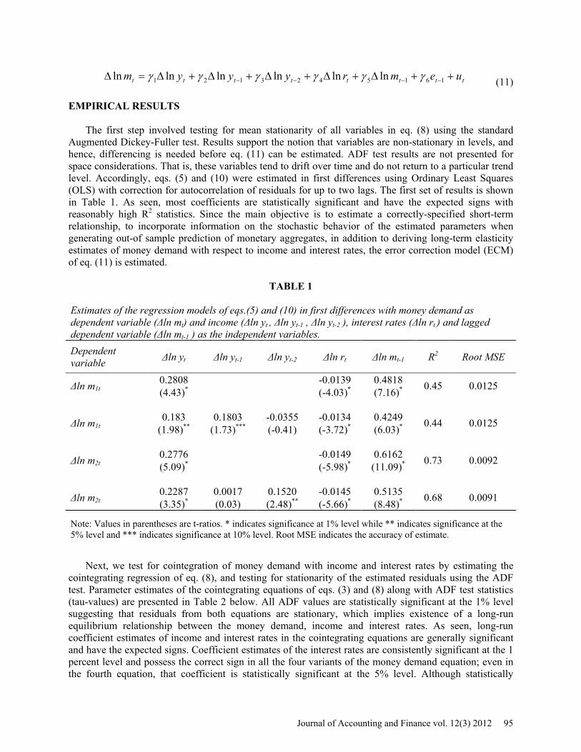
The first step involved testing for mean stationarity of all variables in eq. (8) using the standard Augmented Dickey-Fuller test. Results support the notion that variables are non-stationary in levels, and hence, differencing is needed before eq. (11) can be estimated. ADF test results are not presented for space considerations. That is, these variables tend to drift over time and do not return to a particular trend level. Accordingly, eqs. (5) and (10) were estimated in first differences using Ordinary Least Squares (OLS) with correction for autocorrelation of residuals for up to two lags. The first set of results is shown in Table 1. As seen, most coefficients are statistically significant and have the expected signs with reasonably high R2 statistics. Since the main objective is to estimate a correctly-specified short-term relationship, to incorporate information on the stochastic behavior of the estimated parameters when generating out-of sample prediction of monetary aggregates, in addition to deriving long-term elasticity estimates of money demand with respect to income and interest rates, the error correction model (ECM) of eq. (11) is estimated.

TABLE 1

Estimates of the regression models of eqs.(5) and (10) in first differences with money demand as dependent variable (Δln mt) and income (Δln yt , Δln yt-1 , Δln yt-2 ), interest rates (Δln rt ) and lagged dependent variable (Δln mt-1 ) as the independent variables. Dependent variable Δln yt Δln yt-1 Δln yt-2 Δln rt Δln mt-1 R2 Root MSE

Δln m1t 0.2808 -0.0139 0.4818 0.45 0.0125 (4.43)* (-4.03)* (7.16)*

Δln m1t 0.183 0.1803 -0.0355 -0.0134 0.4249 0.44 0.0125 (1.98)** (1.73)*** (-0.41) (-3.72)* (6.03)*

Δln m2t 0.2776 -0.0149 0.6162 0.73 0.0092 (5.09)* (-5.98)* (11.09)*

Δln m2t 0.2287 0.0017 0.1520 -0.0145 0.5135 0.68 0.0091 (3.35)* (0.03) (2.48)** (-5.66)* (8.48)*

Note: Values in parentheses are t-ratios. * indicates significance at 1% level while ** indicates significance at the 5% level and *** indicates significance at 10% level. Root MSE indicates the accuracy of estimate.

Next, we test for cointegration of money demand with income and interest rates by estimating the

cointegrating regression of eq. (8), and testing for stationarity of the estimated residuals using the ADF test. Parameter estimates of the cointegrating equations of eqs. (3) and (8) along with ADF test statistics (tau-values) are presented in Table 2 below. All ADF values are statistically significant at the 1% level suggesting that residuals from both equations are stationary, which implies existence of a long-run equilibrium relationship between the money demand, income and interest rates. As seen, long-run coefficient estimates of income and interest rates in the cointegrating equations are generally significant and have the expected signs. Coefficient estimates of the interest rates are consistently significant at the 1 percent level and possess the correct sign in all the four variants of the money demand equation; even in the fourth equation, that coefficient is statistically significant at the 5% level. Although statistically


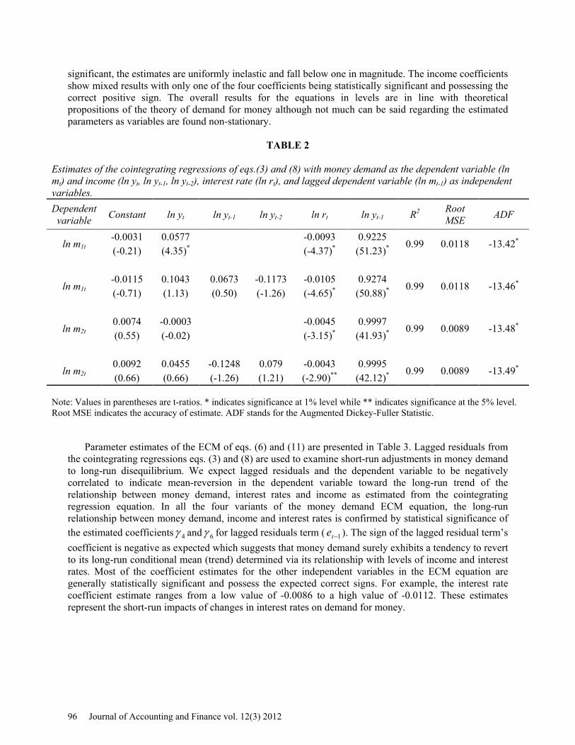
significant, the estimates are uniformly inelastic and fall below one in magnitude. The income coefficients show mixed results with only one of the four coefficients being statistically significant and possessing the correct positive sign. The overall results for the equations in levels are in line with theoretical propositions of the theory of demand for money although not much can be said regarding the estimated parameters as variables are found non-stationary.

TABLE 2

Estimates of the cointegrating regressions of eqs.(3) and (8) with money demand as the dependent variable (ln mt) and income (ln yt, ln yt-1, ln yt-2), interest rate (ln rt), and lagged dependent variable (ln mt-1) as independent variables. Dependent variable Constant ln yt ln yt-1 ln yt-2 ln rt ln yt-1 R2 Root

MSE ADF

ln m1t -0.0031 0.0577 -0.0093 0.9225

0.99 0.0118 -13.42* (-0.21) (4.35)* (-4.37)* (51.23)*

ln m1t -0.0115 0.1043 0.0673 -0.1173 -0.0105 0.9274

0.99 0.0118 -13.46* (-0.71) (1.13) (0.50) (-1.26) (-4.65)* (50.88)*

ln m2t 0.0074 -0.0003 -0.0045 0.9997

0.99 0.0089 -13.48* (0.55) (-0.02) (-3.15)* (41.93)*

ln m2t 0.0092 0.0455 -0.1248 0.079 -0.0043 0.9995

0.99 0.0089 -13.49* (0.66) (0.66) (-1.26) (1.21) (-2.90)** (42.12)*

Note: Values in parentheses are t-ratios. * indicates significance at 1% level while ** indicates significance at the 5% level. Root MSE indicates the accuracy of estimate. ADF stands for the Augmented Dickey-Fuller Statistic.

Parameter estimates of the ECM of eqs. (6) and (11) are presented in Table 3. Lagged residuals from

the cointegrating regressions eqs. (3) and (8) are used to examine short-run adjustments in money demand to long-run disequilibrium. We expect lagged residuals and the dependent variable to be negatively correlated to indicate mean-reversion in the dependent variable toward the long-run trend of the relationship between money demand, interest rates and income as estimated from the cointegrating regression equation. In all the four variants of the money demand ECM equation, the long-run relationship between money demand, income and interest rates is confirmed by statistical significance of the estimated coefficients 4γ and 6γ for lagged residuals term ( 1−te ). The sign of the lagged residual term’s coefficient is negative as expected which suggests that money demand surely exhibits a tendency to revert to its long-run conditional mean (trend) determined via its relationship with levels of income and interest rates. Most of the coefficient estimates for the other independent variables in the ECM equation are generally statistically significant and possess the expected correct signs. For example, the interest rate coefficient estimate ranges from a low value of -0.0086 to a high value of -0.0112. These estimates represent the short-run impacts of changes in interest rates on demand for money.


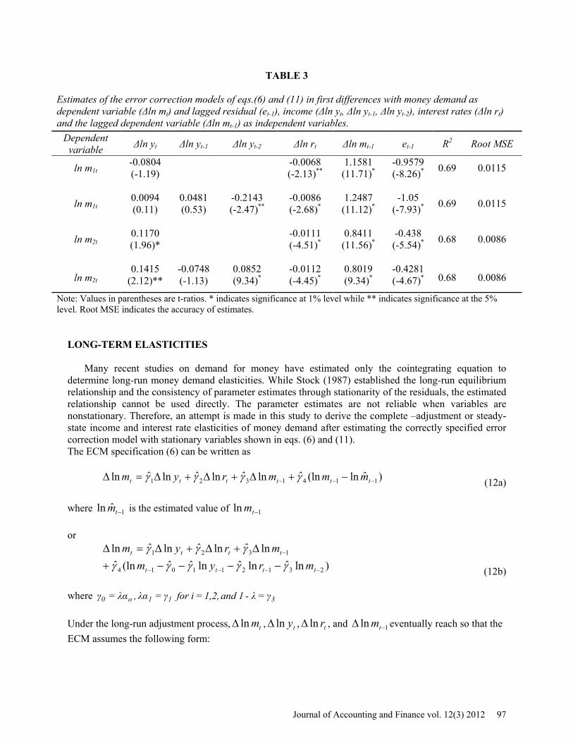
TABLE 3

Estimates of the error correction models of eqs.(6) and (11) in first differences with money demand as dependent variable (Δln mt) and lagged residual (et-1), income (Δln yt, Δln yt-1, Δln yt-2), interest rates (Δln rt) and the lagged dependent variable (Δln mt-1) as independent variables.

Dependent variable Δln yt Δln yt-1 Δln yt-2 Δln rt Δln mt-1 et-1 R2 Root MSE

ln m1t -0.0804 -0.0068 1.1581 -0.9579 0.69 0.0115 (-1.19) (-2.13)** (11.71)* (-8.26)*

ln m1t 0.0094 0.0481 -0.2143 -0.0086 1.2487 -1.05 0.69 0.0115 (0.11) (0.53) (-2.47)** (-2.68)* (11.12)* (-7.93)*

ln m2t 0.1170 -0.0111 0.8411 -0.438 0.68 0.0086 (1.96)* (-4.51)* (11.56)* (-5.54)*

ln m2t 0.1415 -0.0748 0.0852 -0.0112 0.8019 -0.4281

0.68 0.0086 (2.12)** (-1.13) (9.34)* (-4.45)* (9.34)* (-4.67)*

Note: Values in parentheses are t-ratios. * indicates significance at 1% level while ** indicates significance at the 5% level. Root MSE indicates the accuracy of estimates.

LONG-TERM ELASTICITIES

Many recent studies on demand for money have estimated only the cointegrating equation to determine long-run money demand elasticities. While Stock (1987) established the long-run equilibrium relationship and the consistency of parameter estimates through stationarity of the residuals, the estimated relationship cannot be used directly. The parameter estimates are not reliable when variables are nonstationary. Therefore, an attempt is made in this study to derive the complete –adjustment or steady-state income and interest rate elasticities of money demand after estimating the correctly specified error correction model with stationary variables shown in eqs. (6) and (11). The ECM specification (6) can be written as

)ˆln(lnˆlnˆlnˆlnˆln 1141321 −−− −+∆+∆+∆=∆ tttttt mmmrym γγγγ (12a)

where 1ˆln −tm is the estimated value of 1ln −tm or

)lnˆlnˆlnˆˆ(lnˆlnˆlnˆlnˆln

231211014

1321

−−−−

−

−−−−+∆+∆+∆=∆

tttt

tttt

mrymmrymγγγγγ

γγγ

(12b)

where 311o0 γλ-1 and 1,2,i for γλα ,λαγ ==== Under the long-run adjustment process, tmln∆ , tyln∆ , trln∆ , and 1ln −∆ tm eventually reach so that the ECM assumes the following form:


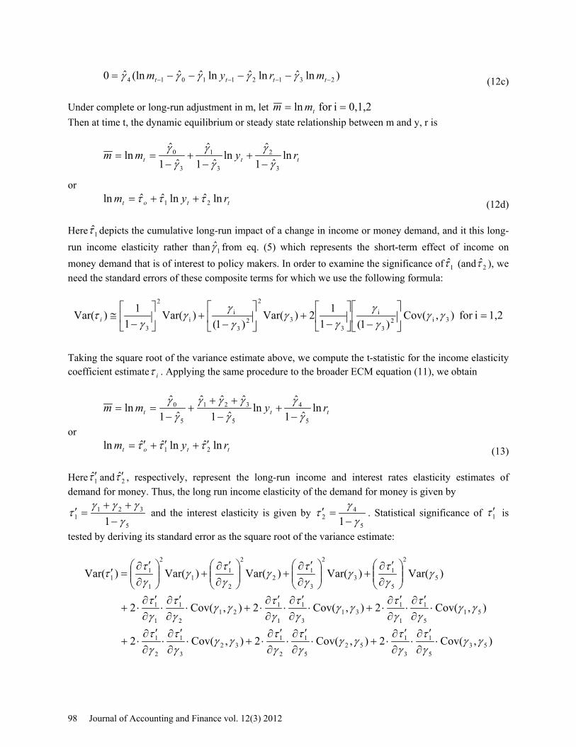
)lnˆlnˆlnˆˆ(lnˆ0 231211014 −−−− −−−−= tttt mrym γγγγγ (12c)

Under complete or long-run adjustment in m, let 0,1,2ifor ln == tmm Then at time t, the dynamic equilibrium or steady state relationship between m and y, r is

ttt rymm lnˆ1

ˆln

ˆ1ˆ

ˆ1ˆ

ln3

2

3

1

3

0

γγ

γγ

γγ

−+

−+

−==

or ttot rym lnˆlnˆˆln 21 τττ ++= (12d)

Here 1̂τ depicts the cumulative long-run impact of a change in income or money demand, and it this long-run income elasticity rather than 1γ̂ from eq. (5) which represents the short-term effect of income on money demand that is of interest to policy makers. In order to examine the significance of 1̂τ (and 2τ̂ ), we need the standard errors of these composite terms for which we use the following formula:

1,2ifor ),Cov( )1(1

12)Var()1(

)Var(1

1)Var( 3i23

i

33

2

23

ii

2

3

=

−

−

+

−

+

−

≅ γγγγ

γγ

γγ

γγ

τ i

Taking the square root of the variance estimate above, we compute the t-statistic for the income elasticity coefficient estimate iτ . Applying the same procedure to the broader ECM equation (11), we obtain

ttt rymm lnˆ1

ˆln

ˆ1ˆˆˆ

ˆ1ˆ

ln5

4

5

321

5

0

γγ

γγγγ

γγ

−+

−++

+−

==

or ttot rym lnˆlnˆˆln 21 τττ ′+′+′= (13)

Here 1̂τ ′ and 2τ̂ ′ , respectively, represent the long-run income and interest rates elasticity estimates of demand for money. Thus, the long run income elasticity of the demand for money is given by

5

3211 1 γ

γγγτ

−++

=′ and the interest elasticity is given by 5

42 1 γ

γτ

−=′ . Statistical significance of 1τ ′ is

tested by deriving its standard error as the square root of the variance estimate:

),Cov(2),Cov(2),Cov(2

),Cov(2),Cov(2),Cov(2

)Var()Var()Var()Var()Var(

535

1

3

152

5

1

2

132

3

1

2

1

515

1

1

131

3

1

1

121

2

1

1

1

5

2

5

13

2

3

12

2

2

11

2

1

11

γγγτ

γτ

γγγτ

γτ

γγγτ

γτ

γγγτ

γτ

γγγτ

γτ

γγγτ

γτ

γγτ

γγτ

γγτ

γγτ

τ

⋅∂

′∂⋅

∂′∂

⋅+⋅∂

′∂⋅

∂′∂

⋅+⋅∂

′∂⋅

∂′∂

⋅+

⋅∂

′∂⋅

∂′∂

⋅+⋅∂

′∂⋅

∂′∂

⋅+⋅∂

′∂⋅

∂′∂

⋅+

∂

′∂+

∂

′∂+

∂

′∂+

∂′∂

=′


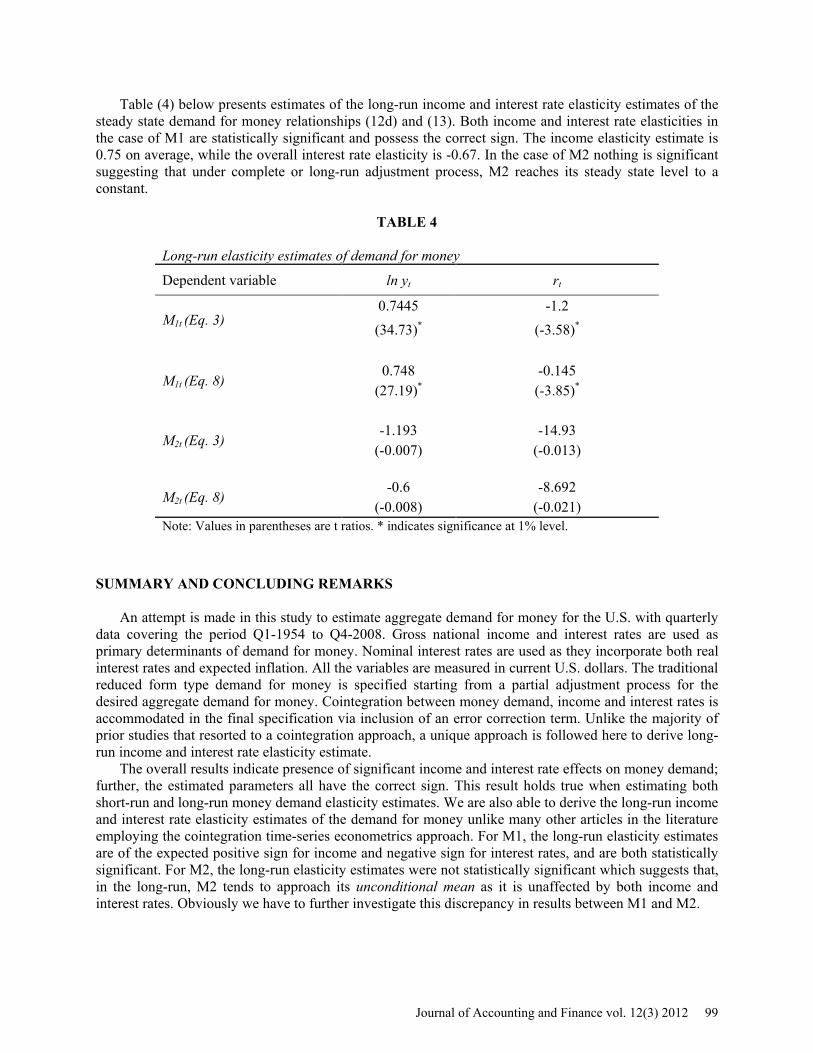
Table (4) below presents estimates of the long-run income and interest rate elasticity estimates of the steady state demand for money relationships (12d) and (13). Both income and interest rate elasticities in the case of M1 are statistically significant and possess the correct sign. The income elasticity estimate is 0.75 on average, while the overall interest rate elasticity is -0.67. In the case of M2 nothing is significant suggesting that under complete or long-run adjustment process, M2 reaches its steady state level to a constant.

TABLE 4

Long-run elasticity estimates of demand for money

Dependent variable ln yt rt

M1t (Eq. 3) 0.7445 -1.2

(34.73)* (-3.58)*

M1t (Eq. 8) 0.748 -0.145

(27.19)* (-3.85)*

M2t (Eq. 3) -1.193 -14.93

(-0.007) (-0.013)

M2t (Eq. 8) -0.6 -8.692

(-0.008) (-0.021) Note: Values in parentheses are t ratios. * indicates significance at 1% level.

SUMMARY AND CONCLUDING REMARKS An attempt is made in this study to estimate aggregate demand for money for the U.S. with quarterly

data covering the period Q1-1954 to Q4-2008. Gross national income and interest rates are used as primary determinants of demand for money. Nominal interest rates are used as they incorporate both real interest rates and expected inflation. All the variables are measured in current U.S. dollars. The traditional reduced form type demand for money is specified starting from a partial adjustment process for the desired aggregate demand for money. Cointegration between money demand, income and interest rates is accommodated in the final specification via inclusion of an error correction term. Unlike the majority of prior studies that resorted to a cointegration approach, a unique approach is followed here to derive long-run income and interest rate elasticity estimate.

The overall results indicate presence of significant income and interest rate effects on money demand; further, the estimated parameters all have the correct sign. This result holds true when estimating both short-run and long-run money demand elasticity estimates. We are also able to derive the long-run income and interest rate elasticity estimates of the demand for money unlike many other articles in the literature employing the cointegration time-series econometrics approach. For M1, the long-run elasticity estimates are of the expected positive sign for income and negative sign for interest rates, and are both statistically significant. For M2, the long-run elasticity estimates were not statistically significant which suggests that, in the long-run, M2 tends to approach its unconditional mean as it is unaffected by both income and interest rates. Obviously we have to further investigate this discrepancy in results between M1 and M2.


ENDNOTES

1. Khan (1974), Laumas and Mehra (1977), Hafer and Hein (1980), Laumas and Spencer (1980), Judd and Scadding (1982), Klovland (1982), Ram and Biswas (1983), Mizrach and Santomero (1986), Fair (1987), Ahmad and Khan (1990), Swamy and Tavlas (1992), Ball (2001), Duca and VanHoose (2004), Rao and Kumar (2007), Choi and Jung (2009), and Hsing and Jamal (2011)

2. Hondroyiannis, Swamy and Tavlas (2001) 3. It is to be noted that the partial adjustment mechanism has been specified both in real as well as in nominal

terms in the literature. It appears that no consensus has emerged in favor of one or the other. 4. The Changes in variables present only short-run effects because they are period to period changes, and

information contained in the levels of the variables about the long-term relationship is lost REFERENCES Ahmad, M. & Ashfaque H. K. (1990). A Reexamination of the Stability of the Demand for Money in Pakistan. Journal of Macroeconomics, 12, (2), Spring, 307-321. Ball, L. (2001). Another Look at Long-Run Money Demand. Journal of Monetary Economics, 47, 31-44. Bose, S. & Rahman H. (1996). The Demand for Money in Canada: A Cointegration Analysis. International Economic Journal, 10, (4), Winter, 29-45. Bronfenbrenner,M. & Mayer, T. (1960). Liquidity Functions in the American Economy. Econometrica, 28, 810-834. Cagan, P. (1956). The Monetary Dynamics of Hyperinflation, in M. Friedman (ed). Studies in the Quantity Theory of Money: The University of Chicago Press, Chicago. Carlson, J.A. (1977). A Study of Price Forecasts. Annals of Economic and Social Measurement, 6, Winter, 27-56. Choi, K. & Chulho, J. (2009). Structural Changes and the US Money Demand Function. Applied Economics, 41, 1251-1257. Chow, G.C. (1966). On the Long-run and Short-run Demand for Money. Journal of Political Economy, 74, April, 111-131. Cooley, T. & Prescott E. (1976). Estimation in the Presence if Stochastic Parameter Variation. Econometrical, 44, 167-184. Deaver, J.V. Chilean Inflation and the Demand for Money in D. Meiselman (ed). Varieties of Monetary Experience: the University of Chicago Press, Chicago. Diz, A. C. (1970) Money and Prices in Argentina 1935-62, in D. Meiselman (ed). Varieties of Monetary Experience, the University of Chicago Press, Chicago. Duca, J. V. & VanHoose, D.D. ( 2004 ). Recent Developments in Understanding the Demand for Money. Journal of Economics and Business, 56, 247-272.


Engle, R. F. & Granger, C. W. J. (1987). Cointegration and Error Correction: Representation, Estimation, and Testing. Econometrica, 55, 251-76. Fackler, J. & Mark W. (1982 ). Recent Instability of the Demand for Money: Some Further Estimates. Southern Economic Journal, 48, April, 1088-1090. Fair, Ray C. (1987 ). International Evidence on the Demand for Money. The Review of Economics and Statistics, 69, (3), August, 473-480. Friedman, M. (1956). The Quantity Theory of Money: A Restatement (ed M. Friedman): the University of Chicago Press, Chicago. Friedman, M. (1959). The Demand for Money: Some Theoretical and Empirical Evidence. Journal of Political Economy 67, 327-351. Freidman, M. (1966). Interest Rates and the Demand for Money. Journal of Law and Economics, 9, October. Goldberger, A.S. (1972). Maximum Likelihood Estimation of Regressions Containing Unobservable Independent Variables. International Economic Review, 13, February, 1-15. Goldfeld, S.M. (1973). The Demand for Money Revisited. Brooklings papers on economic activity, 3, 577-638. Granger, C. W. J. and Newbold, P. Forecasting Economic Time Series, 2nd ed: Academic Press, INC., Orlando, Florida. Drama, B. G. H. & Yao S.. (2001). The Demand for Money in Cote d’Ivoire: Evidence from the Cointegration Test. International Journal of Economics and Finance, 3, (1), February, 188-197. Hafer, R.W., & Scott E. H. (1980).The Dynamics and Estimation of Short-Run Money Demand. Federal Reserve Bank of St. Louis Review, 62, (3), March, 26-35. Hsing, Y. & Jamal A. M. M. (2011).The Demand for Money in a Simultaneous-Equation Framework. Economics Bulletin, 31, 1-5. Hynes, A. (1967).The Demand for Money and Monetary Adjustments in Chile. Review of Economic Studies, 34, 285-293. Judd, J. P., & Scadding J. L. (1982). The Search for a Stable Money Demand Function: A survey of the Post-1973 Literature. Journal of Economic Literature, XX, September, 993-1023. Khan, M. S. (1974). Stability of the Demand-for-Money Function in the United States 1901-1965. Journal of Political Economy, 82, (6), 1205-1219. Klein, B. (1975). The Demand for Quality Adjusted Cash Balances: Price Uncertainty in the U.S. Demand for Money Function. Journal of Political Economy, 85, August, 691-715. Klovland, J. T. (1982). The Stability of the Demand for Money in the Interwar Years. Journal of Money, Credit, and Banking, 14, (2), May, 252-264.


Kolluri, B.R. (1977). Analysis of Econometric Models Containing Unobservable. Ph.D Dissertation (unpublished), Department of Economics, State University of New York at Buffalo, January. Laidler, D.E.W. (1977).The Demand for Money: Theories and Evidence, Dun-Donnelley Publishing Corp. Latane, H.A. (1954). Cash Balances and the Interest Rates: A Pragmatic Approach. Review of Economics and Statistics, 36, 456-460. Latane, H.A. (1960). Income Velocity and Interest Rates: A Pragmatic Approach. Review of Economics and Statistics, 42, 445-449. Laumas, G.S., & Mehra Y.P. (1977). The Stability of the Demand for Money Function 1900-1974. The Journal of Finance, XXXII, (3), June, 911-916. Laumas, G.S., & Spencer D. E. (1980). The Stability of the Demand for Money: Evidence from the Post-1973 Period. The Review of Economics and statistics, 62, (3), August, 455-459. Lybeck, J.A. (1975). Issues in The Theory of the Long-Run Demand for Money. Swedish Journal of Economics, 77, 193-206. Malinvaud. (1970). Statistical Methods of Econometrics, second revised edition, Amsterdam: North-Holland. Melitz, J. (1976). Inflationary Expectations and the French Demand for Money 1959-70. Manchester School, 44, March, 17-41. Mizrach, B., & Santomero M. (1986). The Stability of Money Demand and Forecasting Through Changes in Regimes. The Review of Economics and Statistics, 68, (2), May, 324-28. Quandt, R. (1960). Tests of the Hypothesis that a Linear Regression Obeys Two Separate Regimes. Journal of the American Statistical Association, 55, June, 324-330. Ram, R. (1982). Recent Instability of the Demand for Money: Another Test of Stability. Southern Economic Journal, 48, April, 1083-87. Ram, R., & Biswas B. (1983). Stability of Demand for Money in India: Some Further Evidence. Indian Economic Journal, 31, July-September, 77-88. Rao, B. B. & Kumar, S. (2007). Structural Breaks, Demand for Money and Monetary Policy in Fiji. Pacific Economic Bulletin, 22, 53-62. Shapiro, A.A. (1973). Inflation, Lags, and the Demand for Money. International Economic Review, 14, February, 81-86. Shen C. H. & Huang T. S. (1999). Money Demand and Seasonal Cointegration. International Economic Journal, 13, (3), Autumn, 97-123. Simos, E. O. & Triantis J. E. (1983). Static and Dynamic Forecasting of Short-Run Demand for Money. Technological Forecasting and Social Change, 24, (3), November, 247-254.


Smith, L.B. & Winder, J.W.L. (1971). Price and Interest Rate Expectations and the Demand for Money in Canada. Journal of Finance, 26, 671-682. Stock, J.H. (1987). Asymptotic Properties of Least Squares Estimators of Cointegrating Vectors. Econometrica, 55, 1035-56. Suvanto, A. (1976). Permanent Income, Inflation Expectations and the Long-run Demand for Money in Finland. The Scandinavian Journal of Economics, 78, 457-469. Swamy, P.A.V.B., & Tavlas G. S. (1992). Is it Possible to Find an Econometric Law that Works Well in Explanation and Prediction? The Case of Australian Money Demand. Journal of Forecasting, 11, 17-33. Swamy, P.A.V.B., Kolluri B.R. & Singamsetti R.N. (1990).What Do Regressions of Interest Rates on Deficits Imply? Southern Economic Journal, 56, 1010-28. Swamy, P.A.V.B., Kennickell A.B. & von zur Muehlen P. (1990). Comparing Forecasts from Fixed and Variable Coefficient Models: The Case of Money Demand. International Journal of Forecasting, 6, 469-477. Turnovsky, S. J. (1970). Some Empirical Evidence on the Formation of Price Expectations. Journal of the American Statistical Association, 65, December, 1441-1454. Zellner, A. (1970). Estimation of Regression Relationships Containing Unobservable Independent Variables. International Economic Review, 11, October 441-454.


Documents

Short-Run and Long-Run Money Demand: Recent Evidence · Short-Run and Long-Run Money Demand: Recent Evidence Bharat R. Kolluri University of Hartford Rao Singamsetti University of