Embed Size (px)
Citation preview
SIGNAL CLASSIFICATION THROUGH MULTIFRACTAL ANALYSIS AND NEURAL NETWORKS
by
Kevin Cannons
Vincent Cheung
A Thesis submitted to the University of Manitoba in Partial Fulfillment of
the Requirements for the Degree of
BACHELOR OF SCIENCE
Department of Electrical and Computer Engineering
University of Manitoba
Winnipeg, Manitoba, Canada
Thesis Advisor: W. Kinsner, Ph. D., P. Eng.
March 2003

SIGNAL CLASSIFICATION THROUGH MULTIFRACTAL ANALYSIS AND NEURAL NETWORKS
by
Kevin Cannons
Vincent Cheung
A Thesis submitted to the University of Manitoba in Partial Fulfillment of
the Requirements for the Degree of
BACHELOR OF SCIENCE
Department of Electrical and Computer Engineering
University of Manitoba
Winnipeg, Manitoba, Canada
Thesis Advisor: W. Kinsner, Ph. D., P. Eng.
© K. Cannons, V. Cheung; March 2003
(vii + 89 + A-4 + B-5 + C-1) = 106 pp.
- i -

- ii -
ABSTRACT
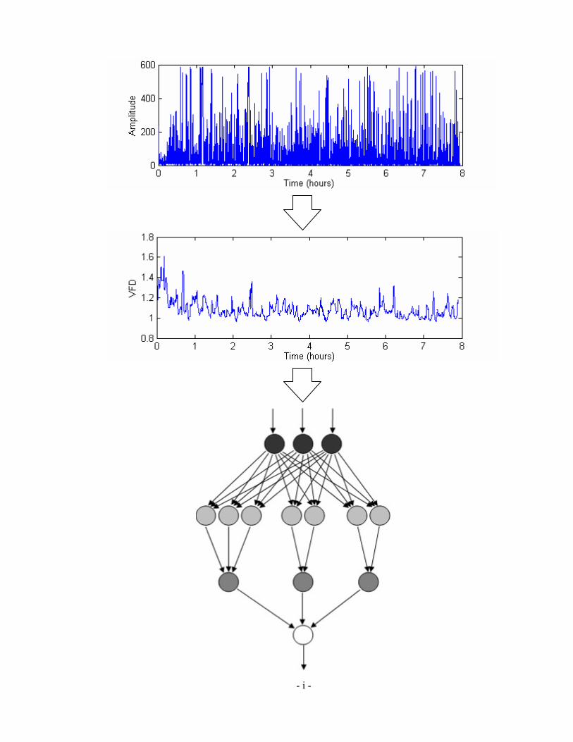
This thesis proposes a method of classifying stochastic, non-stationary, self-similar
signals which originate from non-linear systems and may be comprised of multiple signals, using
a multifractal analysis and neural networks.
The first stage of the signal classification process entails the extraction of the most
important features of the signal. To perform this feature extraction, the signal is first transformed
into the fractal dimension domain by calculating its variance fractal dimension trajectory
(VFDT). This transformation emphasizes the underlying multifractal characteristics of the signal,
and more importantly for classification, it produces a normalized signal. The resulting VFDT can
be used directly for classification. Alternatively, the most important features of the VFDT can be
obtained through the use of Kohonen self-organizing feature maps (SOFMs) and the classification
can then be based upon these features. Configurations with and without the SOFMs are examined
in this thesis.
The second stage of the classification process involves the use of neural networks to
determine the particular class of a signal based on its extracted features. This thesis employs
several advanced neural networks, including probabilistic neural networks (PNNs) and complex
domain neural networks (CNNs). While the use of PNN has been sparse in previous research, it
has significant advantages over traditional neural networks, including faster training times and
classification accuracies that are asymptotically Bayes optimal. Similarly, CNNs have not been
used extensively, but research in the area has shown that they often generalize more effectively
than real domain networks. Additionally, these networks are able to take advantage of the strong
correlation between multiple signals that constitute an entire signal.
The classification system implemented in this thesis is verified using spatio-temporal
recordings of a Siamese fighting fish when presented with various stimuli during dishabituation
experiments in a fish tank. The experiments performed in this thesis show that the proposed
classification systems are capable of classifying non-stationary, self-similar signals, such as the
fish trajectory signal, with accuracies up to 90%. Additionally, the experiments verified that the
use of multiple signal components of the fish trajectory signal yield better results than when only
a single component is used.

- iii -
ACKNOWLEDGEMENTS
We would like to thank Dr. Kinsner for his continued support and encouragement while
working on our thesis. Additionally, we would further like to thank Dr. Kinsner for introducing
us to our thesis topic, through which we have broadened and enriched our knowledge base well
beyond what we would have otherwise achieved in our undergraduate studies.
We would also like to thank the members of the Delta Research Group, especially Robert
Barry, Kalen Brunham, Stephen Dueck, Hakim El-Boustani, Aram Faghfouri, Neil Gadhok, Bin
Huang, Michael Potter, Leila Safavian, and Sharjeel Siddiqui, as well as our families and friends
for all their helpful suggestions and words of encouragement.
Many thanks must also be expressed to Dr. Pear and his research group for supplying us
with the fish trajectory signals for use in this thesis.
Finally, we would like to express our sincere gratitude to the Natural Sciences and
Engineering Research Council of Canada and the University of Manitoba for their financial
support of the research performed for this thesis.

- iv -
TABLE OF CONTENTS
Abstract ...................................................................................................... ii
Acknowledgements ................................................................................... iii
List of Figures ........................................................................................... vi
List of Tables............................................................................................ vii
Chapter 1 Introduction.............................................................................. 1 1.1 Purpose .......................................................................................................................... 1 1.2 Problem.......................................................................................................................... 1 1.3 Scope ............................................................................................................................. 2 1.4 Thesis Organization........................................................................................................ 2
Chapter 2 Background .............................................................................. 4 2.1 Signal Classification and Terminology ........................................................................... 4 2.2 Fractals .......................................................................................................................... 6
2.2.1 Introduction ....................................................................................................... 7 2.2.2 Variance Fractal Dimension ............................................................................... 9
2.3 Neural Networks .......................................................................................................... 13 2.3.1 Introduction ..................................................................................................... 13 2.3.2 Basic Concepts ................................................................................................ 14 2.3.3 Backpropagation .............................................................................................. 19 2.3.4 Complex Domain Neural Networks.................................................................. 22 2.3.5 Probabilistic Neural Networks.......................................................................... 24 2.3.6 Kohonen Self-Organizing Feature Maps........................................................... 33
2.4 Summary...................................................................................................................... 35
Chapter 3 System Design..........................................................................36 3.1 System Architecture ..................................................................................................... 36 3.2 Component Design ....................................................................................................... 40
3.2.1 Preprocessing................................................................................................... 40 3.2.2 Variance Fractal Dimension Trajectory ............................................................ 41 3.2.3 Kohonen Self-Organizing Feature Map ............................................................ 43 3.2.4 Probabilistic Neural Network ........................................................................... 46 3.2.5 Complex Domain Neural Network ................................................................... 48
3.3 Summary...................................................................................................................... 50
Chapter 4 System Implementation ..........................................................51 4.1 System ......................................................................................................................... 51 4.2 Component................................................................................................................... 52
4.2.1 Preprocessing................................................................................................... 52 4.2.2 Variance Fractal Dimension Trajectory ............................................................ 53 4.2.3 Kohonen Self-Organizing Feature Map ............................................................ 54 4.2.4 Probabilistic Neural Network ........................................................................... 55
- v -
4.2.5 Complex Domain Neural Network ................................................................... 58 4.2.6 Input Vector Creation....................................................................................... 59 4.2.7 Classifier Driver .............................................................................................. 61
4.3 Summary...................................................................................................................... 62
Chapter 5 System Verification and Testing.............................................63 5.1 Component Verification and Testing ............................................................................ 63
5.1.1 Preprocessing................................................................................................... 63 5.1.2 Variance Fractal Dimension Trajectory ............................................................ 63 5.1.3 Kohonen Self-Organizing Feature Map ............................................................ 64 5.1.4 Probabilistic Neural Network ........................................................................... 65 5.1.5 Complex Domain Neural Network ................................................................... 68
5.2 Overall System Verification and Testing....................................................................... 68 5.3 Summary...................................................................................................................... 69
Chapter 6 Experimental Results and Discussion ....................................70 6.1 Experiment Set-Up ....................................................................................................... 70 6.2 Results ......................................................................................................................... 75
6.2.1 Experiment 1: X-Axis with PNN..................................................................... 75 6.2.2 Experiment 2: X-Axis with SOFM and PNN................................................... 77 6.2.3 Experiment 3: Z-Axis with PNN ..................................................................... 78 6.2.4 Experiment 4: Z-Axis with SOFM and PNN ................................................... 79 6.2.5 Experiment 5: X and Z-Axis with PNN ........................................................... 80 6.2.6 Experiment 6: X and Z-Axis with SOFM and PNN ......................................... 81 6.2.7 Experiment 7: X and Z-Axis with CNN........................................................... 81 6.2.8 Experiment 8: X and Z-Axis with SOFM and CNN......................................... 82
6.3 Discussion.................................................................................................................... 83 6.4 Summary...................................................................................................................... 85
Chapter 7 Conclusions and Recommendations .......................................86 7.1 Conclusions.................................................................................................................. 86 7.2 Recommendations ........................................................................................................ 86
References .................................................................................................88
Appendix A Fish Trajectory Signals..................................................... A-1
Appendix B Clustering of Fish Trajectory Signals ...............................B-1
Appendix C Source Code....................................................................... C-1

- vi -
LIST OF FIGURES
Fig. 2.1: The Koch curve fractal at various magnifications. ........................................................ 7 Fig. 2.2: A hexagon viewed at different magnifications. ............................................................. 8 Fig. 2.3: A multilayer feedforward neural network. .................................................................. 14 Fig. 2.4: The basic operation of a neuron. ................................................................................. 16 Fig. 2.5: Mutually exclusive training and testing sets. ............................................................... 18 Fig. 2.6: Correct classification rate as a function of sigma,σ. .................................................... 27 Fig. 2.7: Basic architecture of a PNN........................................................................................ 28 Fig. 3.1: System block diagram. ............................................................................................... 37 Fig. 3.2: VFDT log-log plots and frequency spectrum plots. ..................................................... 42 Fig. 4.1: Preprocessing UML class diagram.............................................................................. 52 Fig. 4.2: SignalReader UML class diagram. ............................................................................. 52 Fig. 4.3: Variance fractal dimension trajectory UML class diagram. ......................................... 53 Fig. 4.4: Kohonen self-organizing feature map UML class diagram.......................................... 54 Fig. 4.5: Probabilistic neural network UML class diagram........................................................ 55 Fig. 4.6: Sectioning sigma optimization UML class diagram. ................................................... 57 Fig. 4.7: Conjugate gradient sigma optimization UML class diagram........................................ 58 Fig. 4.8: Complex domain neural network UML class diagram................................................. 59 Fig. 4.9: Create input vectors UML class diagram. ................................................................... 60 Fig. 4.10: Classifier driver UML class diagram. ....................................................................... 61 Fig. 5.1: Erroneous selection of bounded minimum. ................................................................. 67 Fig. 6.1: Time domain plots of a fish trajectory signal. ............................................................. 71 Fig. 6.2: VFDTs of a fish trajectory signal................................................................................ 72 Fig. 6.3: MSE histogram of the VFDT of the fish trajectory signal. .......................................... 73 Fig. 6.4: VFDT segment and its codebook. ............................................................................... 75 Fig. A.1: Fish trajectory signal experiment set-up and fish tank co-ordinate system. ............... A-1 Fig. A.2: Fish trajectory signals.............................................................................................. A-2 Fig. B.1: Clustering Codebook. .............................................................................................. B-3 Fig. B.2: Euclidean Distance Between Codewords ................................................................. B-3

- vii -
LIST OF TABLES
Table 6.1: X-axis PNN confusion matrix. ................................................................................. 75 Table 6.2: X-axis SOFM PNN confusion matrix....................................................................... 77 Table 6.3: Z-axis PNN confusion matrix. ................................................................................. 78 Table 6.4: Z-axis SOFM PNN confusion matrix. ...................................................................... 79 Table 6.5: X and Z-axis PNN confusion matrix. ....................................................................... 80 Table 6.6: X and Z-axis SOFM PNN confusion matrix............................................................. 81 Table 6.7: X and Z-axis CNN confusion matrix........................................................................ 82 Table 6.8: X and Z-axis SOFM CNN confusion matrix. ........................................................... 83

Chapter 1: Introduction
- 1 -
CHAPTER 1
INTRODUCTION
1.1 Purpose
The goal of this thesis is to develop a software system that is capable of classifying
stochastic, self-similar, non-stationary signals which originate from non-linear systems.
Complicated signals such as these are often composed of multiple signals, and the system for this
thesis will have the ability to take these multiple signals into account during the classification
process.
This thesis is unique because of the particular techniques that that are chosen to perform
the classification. Specifically, a rarely used transformation is used to represent a signal by its
variance fractal dimensions. This translation emphasizes the underlying multifractal
characteristics of the signal, and more importantly for classification, it has a normalizing effect.
Once the most significant features are extracted through the multifractal analysis, two advanced
neural networks are explored to perform the actual classification. One of the neural networks
utilized in this thesis is the probabilistic neural network. While the use of this network has been
sparse in previous research, it has significant advantages over traditional multilayer feedforward
neural networks including faster training times and classification accuracies that are
asymptotically Bayes optimal. The second neural network used for classification is the complex
domain neural network. This network has yet to be used extensively in research or practice, but it
is often able to generalize more effectively than real domain neural networks and is able to take
full advantage of the multiple signals that constitute an overall signal.
1.2 Problem
Signal classification is the analysis of a signal whereby the signal is determined to belong
to a particular class based on certain characteristic features. The membership to a particular class
usually signifies something about the physical process or system from whence the signal
originated. The classification and analysis of stochastic, non-stationary, self-similar signals
produced by non-linear systems is important because many real world processes have been shown
to generate signals of this type. The nature of these signals makes them very challenging to

Chapter 1: Introduction
- 2 -
analyze because traditional techniques, such as the Fourier transform, which often depend on the
stationarity of a signal and the linearity of the analyzed system, cannot be applied. In addition to
belonging to the class of stochastic, self-similar signals, non-stationary signals, many signals that
are produced in the real world consist of multiple signals that are required to completely define
the overall signal. For example, multichannel audio signals and multiple lead
electroencephalograms and electrocardiograms all consist of many signals, all of which are
required to provide a complete description of the physical process from which they were created.
Since traditional techniques cannot effectively be applied to these types of complex
signals, more advanced methods are sought. The first task that is usually undertaken in an
attempt to classify these complex signals is to extract the most important characteristics, or
features from the signal. In general, the fewest number of features that are capable of
representing the different classes of signals are desired. Once the most important features have
been extracted from the signal, they are used to determine the class membership of the signal.
The function that maps these input features to an output class is often unknown and very
complex. As a result, sophisticated classification methods are required to determine to what class
the signal belongs based on its given features.
1.3 Scope
This paper will limit the feature extraction to utilizing a multifractal characterization
through the computation of the variance fractal dimension trajectory in addition to Kohonen self-
organizing feature maps. The classifiers used to perform the classification based on these
features are restricted to probabilistic and complex domain neural networks. The differing
degrees of success of the various configurations of the system will be measured through the use
of fish trajectory signals in which only two components of the signal are considered.
1.4 Thesis Organization
This paper is divided into seven distinct chapters. Chapter 1 provides a general
introduction to the thesis and outlines its motivation and objectives. Chapter 2 gives background
information on the different techniques that are used in the thesis. The third and fourth chapters
describe the design and implementation of the classification system. The fifth chapter details the
testing and verification methods used to ensure that the software components operate as expected.

Chapter 1: Introduction
- 3 -
Chapter 6 explains the experiments performed to gauge the performance of the classification
system and thoroughly discuss their results and implications. Chapter 7 concludes the thesis and
suggests future work that can extend the work done in this thesis to improve the performance of
the system. Appendices A and B provide a description of the fish trajectory signals used to verify
the classification system and the clustering technique used to derive the training and testing sets
for classification. The source code and documentation for the classification system are contained
in Appendix C.

Chapter 2: Background
- 4 -
CHAPTER 2
BACKGROUND
2.1 Signal Classification and Terminology
This section provides a general description of the overall idea of signal classification and
introduces the terms used to describe the types of signals used in this thesis.
Before proceeding any further into this thesis, the concept of signal classification must
first be concretely defined. Signal classification means to analyze different characteristics of a
signal, and based on those characteristics, decide to which grouping or class the signal belongs.
The resulting classification decision can be mapped back into the physical world to reveal
information about the physical process that created the signal. Often, when signal classification is
performed, it is not the goal to determine to which class an entire signal belongs. Instead, a signal
is usually provided where it is known that a variety of different classes exist at different points
throughout the signal. For example, if the signal under analysis is represented in the time
domain, the purpose of classification might be to determine that the first 15 minutes of the signal
belong to class B, while the next fifteen minutes belong to class A, and so on. In this case, all the
principles behind classification remain the same as when the entire signal is classified, but instead
of classifying the whole signal, only a segment of the signal is classified.
In order to perform classification upon signals, several analysis techniques are typically
performed. First, the characteristics or features upon which the signal is to be classified must be
defined. There are an infinite number of features that could be extracted from the signal for the
purpose of classification, including the mean of the signal, its Fourier coefficients, and its wavelet
coefficients [Mall98]. Based on the selected signal features, a classifier will determine to which
class the signal belongs. The output of the classification system, in which the class membership
of the input signal is determined, can then be used to infer what event in the real world process
occurred to produce the input signal. In this thesis, multifractal analysis and Kohonen self-
organizing feature maps (SOFMs) are used to extract the critical features from signals, while
neural networks are the tools used to perform the classification.
It may seem like overkill to use complicated techniques such as multifractal analysis and
SOFMs to extract the important features from the signals when much simpler metrics such as the

Chapter 2: Background
- 5 -
mean and Fourier coefficients of the signal could be used. However, these complex feature
extraction and classification tools are required for this thesis because of the nature of the signals
being classified. Specifically, the signals under analysis in this thesis are non-stationary,
stochastic, self-similar signals that originate from non-linear systems. These terms describe very
complex signals and may not commonly be known, hence they will each be briefly defined.
The term non-stationary, in the general sense, means that the statistical properties of a
signal change over time. More specifically, properties such as the signal’s mean, variance,
kurtosis, and skewness do not remain constant over the entire duration of the signal, but rather,
change from one point in the signal to the next. A standard sine wave, for example, would be
considered a stationary signal as its statistics remain constant. The statistics for other signals,
such as those produced by speech, clearly do not remain constant, making them non-stationary.
Although an overall signal may not be stationary, usually smaller windows, or parts of those
signals will exhibit stationarity. For example, there is a maximum speed at which the vocal
chords of a human’s voice box can change the sound which they are producing. As a result, a
voice signal is stationary for that small amount of time during which it is physically impossible
for the vocal chords to change sounds. Knowledge of the period over which a particular type of
signal remains stationary is very valuable during signal analysis.
Stochastic refers to signals where the events in the signal occur in a random fashion and
self-similar, at the simplest level means that if a portion of a signal is magnified, the magnified
signal will look the same and have the same statistical properties as the original signal.
Linear systems are systems that abide by the principle of superposition. Most systems in
the real world are decisively non-linear meaning that superposition does not apply. For example,
humans are non-linear systems. Consider a situation where a person is told to perform a chore
and then correspondingly does so. If that same person was yelled at twice as loud to carry out
that same duty, he or she would not necessarily complete the task twice as fast.
Non-stationary, stochastic, self-similar signals originating from non-linear systems are
challenging to analyze, but what makes matters even more complicated is that these signals are
often composed of multiple different recordings, each of which contribute to the information
content of the overall physical phenomena which created the signal. Examples of such signals
include multichannel audio signals and multiple lead electroencephalograms and
electrocardiograms. A classification system can choose to ignore the fact that multiple recordings

Chapter 2: Background
- 6 -
are required to completely define such signals and merely perform classification using the
recording which is deemed the most important. On the other hand, a classification system, such
as the one developed in this thesis, can make use of the information held within the different
recordings in an attempt to achieve superior results.
The goal of this thesis is not the analysis of a particular signal, rather it is the
development of a general classification system which can be used to perform analysis upon non-
stationary, stochastic, self-similar signals originating from non-linear processes. However, in
order to verify the operation of the classification system and gauge its performance, fish
trajectory signals are used. These signals are the result of tracking the three-dimensional position
of a fish in a fish tank when presented with various stimuli over an eight hour period. The fish
signals exhibit the desired stochastic, self-similar, non-stationary properties and originate from a
non-linear system – a fish. The fish trajectory signals also are composed of multiple recordings,
one for each of the Cartesian co-ordinate axes so that the effects of utilizing multiple recordings
during classification can be studied. Sample plots of these signals are shown in Fig. A.2 in
Appendix A. The details of the experiment that generated these signals and a discussion of these
plots are also provided in Appendix A.
2.2 Fractals
This section introduces some of the fundamental concepts behind fractals, and explains
how a specific fractal dimension, the variance fractal dimension, is calculated. By computing the
variance fractal dimension in a sliding-window fashion over an entire signal, a multifractal
analysis is performed whereby a variance fractal dimension trajectory (VFDT) for that signal can
be created. It is the samples in this signal representing the fractal dimensions of the original
signal which is used as the features from which to perform classification. The use of the VFDT
technique has been fairly limited thus far; however, the benefits of its use are significant. The
VFDT representation of the signal can assist in revealing the underlying characteristics of a signal
which may not have been apparent when analyzing the original signal, while simultaneously
compressing the signal into a more compact representation. Being able to reduce the number of
points needed to represent a signal is an invaluable procedure as it makes the classification
process for a classifier much more practical. Most importantly, the resulting VFDT
representation of a signal is normalized, which is essential for the classification based on these
extracted features.

Chapter 2: Background
- 7 -
2.2.1 Introduction
The first notion that must be understood in regards to fractals is that in the simplest sense,
fractals are self-similar entities. As previously defined, self-similarity means that no matter what
magnification is used when viewing an object, its statistical properties, structure, and complexity
remain constant [Mand82]. For example, consider the Koch curve, which is displayed in Fig. 2.1.
The lower of the two images shown is the standard Koch curve. If the upper portion of
the Koch curve is magnified, the resulting image looks identical to the original Koch curve itself,
as can be seen in the upper image of the figure. Mathematically, even if a portion of the Koch
curve is repeatedly magnified, it will still look identical to the original, unmagnified curve.
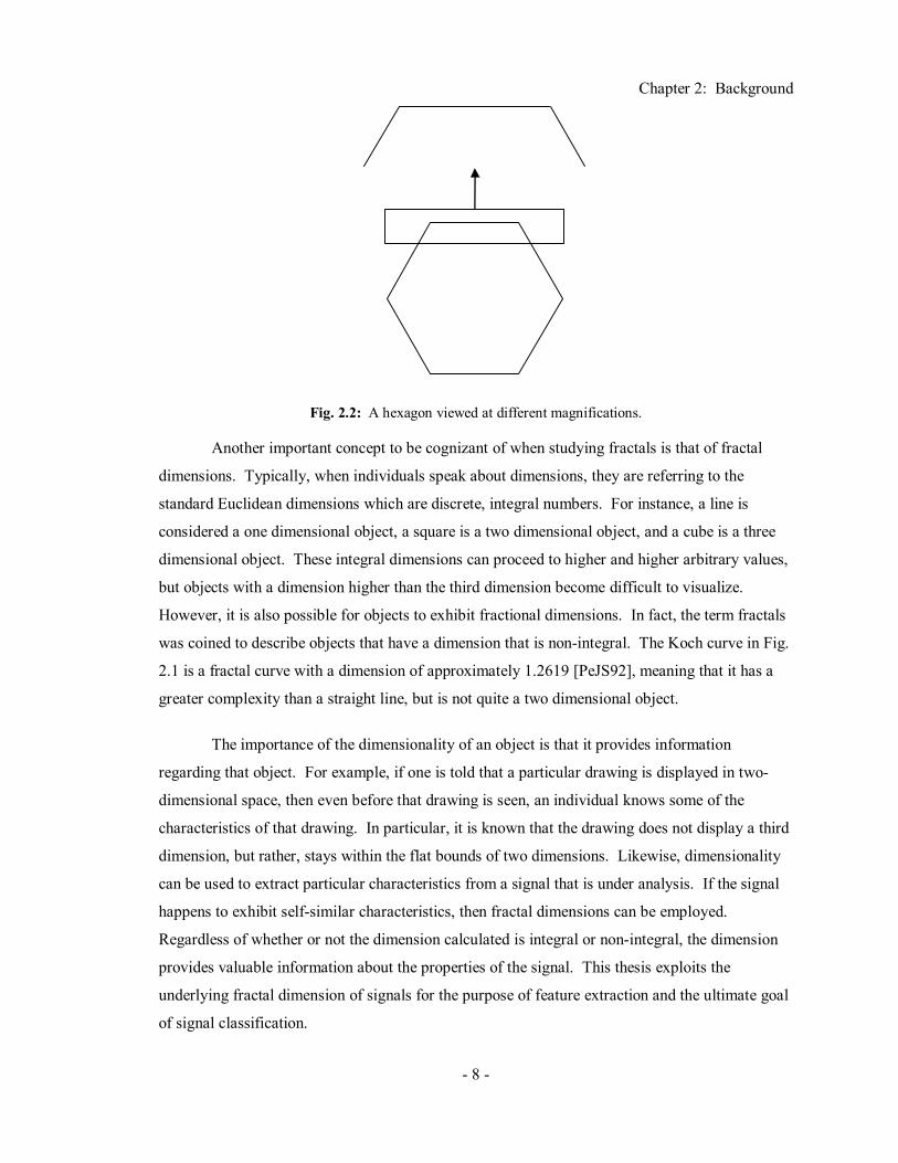
The idea of an object looking the same regardless of what magnification it is viewed
under is quite a contrast to the way most shapes and objects appear when magnified. For
example, if the upper portion of a hexagon is magnified, as shown in Fig. 2.2, the magnified
portion does not look similar to the original, unmagnified hexagon. Typically, as a portion of a
non-fractal object is magnified repeatedly, its complexity will decrease to the point where the
magnified portion will merely appear as a straight line. With fractal objects, this is not the case.
For example, the appearance and complexity of the Koch curve remains constant no matter the
level of magnification used for viewing.
1 Adapted from http://www.jimloy.com/fractals/koch.htm last checked March 6, 2003
Fig. 2.1: The Koch curve fractal at various magnifications.1
Chapter 2: Background
- 8 -
Another important concept to be cognizant of when studying fractals is that of fractal
dimensions. Typically, when individuals speak about dimensions, they are referring to the
standard Euclidean dimensions which are discrete, integral numbers. For instance, a line is
considered a one dimensional object, a square is a two dimensional object, and a cube is a three
dimensional object. These integral dimensions can proceed to higher and higher arbitrary values,
but objects with a dimension higher than the third dimension become difficult to visualize.
However, it is also possible for objects to exhibit fractional dimensions. In fact, the term fractals
was coined to describe objects that have a dimension that is non-integral. The Koch curve in Fig.
2.1 is a fractal curve with a dimension of approximately 1.2619 [PeJS92], meaning that it has a
greater complexity than a straight line, but is not quite a two dimensional object.
The importance of the dimensionality of an object is that it provides information
regarding that object. For example, if one is told that a particular drawing is displayed in two-
dimensional space, then even before that drawing is seen, an individual knows some of the
characteristics of that drawing. In particular, it is known that the drawing does not display a third
dimension, but rather, stays within the flat bounds of two dimensions. Likewise, dimensionality
can be used to extract particular characteristics from a signal that is under analysis. If the signal
happens to exhibit self-similar characteristics, then fractal dimensions can be employed.
Regardless of whether or not the dimension calculated is integral or non-integral, the dimension
provides valuable information about the properties of the signal. This thesis exploits the
underlying fractal dimension of signals for the purpose of feature extraction and the ultimate goal
of signal classification.
Fig. 2.2: A hexagon viewed at different magnifications.
Chapter 2: Background
- 9 -
2.2.2 Variance Fractal Dimension
To further consider the ideas that dimensions need not be integral and that fractal objects
typically possess non-integral dimensions, the process of calculating the dimensionality of an
entity must be explained. Complicating matters is the fact that there are many different types of
dimension. These include topological dimension, box-counting dimension, as well as many
others [PeJS92]. In certain cases the different types of dimensionality, when calculated, yield the
same result for the same object. However, at other times, the computation of the different
dimensions provides different numerical values. For the purposes of this paper, only one form of
fractal dimension, the variance fractal dimension [Kins94], is utilized.
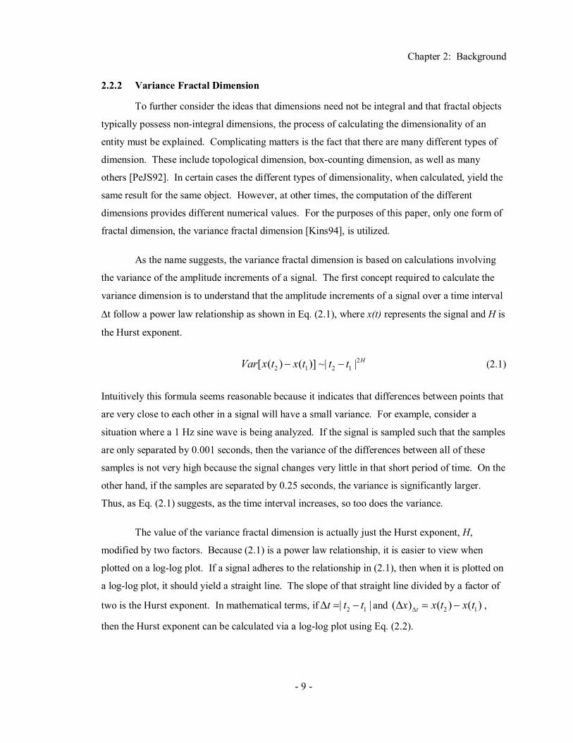
As the name suggests, the variance fractal dimension is based on calculations involving
the variance of the amplitude increments of a signal. The first concept required to calculate the
variance dimension is to understand that the amplitude increments of a signal over a time interval
∆t follow a power law relationship as shown in Eq. (2.1), where x(t) represents the signal and H is
the Hurst exponent.
22 1 2 1[ ( ) ( )] ~| | HVar x t x t t t− − (2.1)
Intuitively this formula seems reasonable because it indicates that differences between points that
are very close to each other in a signal will have a small variance. For example, consider a
situation where a 1 Hz sine wave is being analyzed. If the signal is sampled such that the samples
are only separated by 0.001 seconds, then the variance of the differences between all of these
samples is not very high because the signal changes very little in that short period of time. On the
other hand, if the samples are separated by 0.25 seconds, the variance is significantly larger.
Thus, as Eq. (2.1) suggests, as the time interval increases, so too does the variance.
The value of the variance fractal dimension is actually just the Hurst exponent, H,
modified by two factors. Because (2.1) is a power law relationship, it is easier to view when
plotted on a log-log plot. If a signal adheres to the relationship in (2.1), then when it is plotted on
a log-log plot, it should yield a straight line. The slope of that straight line divided by a factor of
two is the Hurst exponent. In mathematical terms, if 2 1| |t t t∆ = − and 2 1( ) ( ) ( )tx x t x t∆∆ = − ,
then the Hurst exponent can be calculated via a log-log plot using Eq. (2.2).

Chapter 2: Background
- 10 -
0
log[ ( ) ]1lim2 log( )
t
t
Var xHt
∆
→
∆=
∆ (2.2)
As mentioned previously, the variance fractal dimension is merely the Hurst exponent modified
by two factors, which is shown in Eq. (2.3), where Dσ is the variance fractal dimension, and E is
the Euclidean dimension.
1D E Hσ = + − (2.3)
The Euclidean dimension is equal to the number of independent variables in the signal. Thus,
since this thesis concentrates solely upon Euclidean one-dimensional signals, E can be set to 1.
Equation (2.3) then reduces to:
2D Hσ = − (2.4)
The variance fractal dimension can be calculated repeatedly over the duration of a signal
to compute the variance fractal dimension trajectory of the signal. The process of calculating the
VFDT of a signal essentially involves breaking up the entire signal into numerous sub-signals, or
windows, and calculating the variance fractal dimension for each of these windows. The
concatenation of all these fractal dimensions to form a signal is the signal’s VFDT.
A multifractal signal is a signal whose fractal dimension changes over time. Conversely,
a simple fractal signal’s fractal dimension remains constant. The process of computing a signal’s
VFDT is a multifractal characterization as it will expose if a signal contains multiple fractal
dimensions. Should the VFDT be computed upon a simple fractal signal, then the resulting
VFDT is simply constant. There are several benefits in representing a signal in the fractal domain
including dimensionality reduction, underlying feature exemplification, and normalization.
Keeping in mind that the VFDT merely involves taking a signal and transforming it so
that it is represented in the multifractal domain, the following steps [Kins94] outline the
procedure used to calculate the variance fractal dimension trajectory of a signal:

Chapter 2: Background
- 11 -
1. Select values for the window size, NT, and window displacement, d. The window size is
the number of points that are held in each of the smaller sub-signals for which the
variance fractal dimension is calculated. The size of the window should be selected
based on the stationarity of the signal under analysis. The displacement indicates how far
the window shifts following each variance fractal dimension calculation, and determines
the resolution of the resulting VFDT. Both the window and displacement parameters
have an effect on the number of points in the VFDT. A high resolution is usually desired,
indicating a smaller displacement should be used. However, the displacement should not
be given an extremely small value since this would result in significant windowing
artifacts because of the excessive correlation between windows.
2. Next, the change in magnitude, x∆ , is required in order to calculate the Hurst exponent,
as seen in Eq. (2.2). Additionally, as the equation indicates, the time period over which
x∆ is being calculated must be specified. In (2.2) the difference in time was indicated
by t∆ . However, when implementing the VFDT algorithm, the signal being worked with
is digitized and hence the separation should be presented by the number of samples rather
than time. Hence, the number of samples separating two points for which x∆ is
calculated is called nk, and is set as follows:
2 , 1kkn k= > (2.5)
The base of 2 in Eq. (2.5) can be any integer number greater than zero. For this thesis
only a value of 2 is considered. Thus, nk will take on the values of 2, 4, 8, 16, and so on
as k is incremented.
3. Determine the maximum allowable separation, nKhi, between two points for which x∆ can
be calculated by using the following formula:
log log 30log 2 log 2
Thi
NK
= −
(2.6)
The first factor in Eq. (2.6) ensures that the two points remain within the bounds of the
current window. However, if the first factor were left by itself, then the two maximally
separated points for which x∆ is calculated would cover almost the entire window. Thus,
in order to remain statistically valid, there must be room in the window for at least 30
non-overlapping, distinct x∆ intervals. The subtraction factor in (2.6) ensures that the

Chapter 2: Background
- 12 -
maximum allowable separation of the two points involved in the x∆ calculations stays
small enough so that at least 30 x∆ calculations can be performed within the window.
4. Determine the minimum allowable separation between two points, Klow, for which x∆ is
calculated. In order to ensure that the correlation between adjacent values is not too
strong, Klow must be a value greater than 1.
5. Create a pointer indicating the beginning of the current window.
6. Position the pointer to the beginning of the signal.
7. Let the first NT points following the position pointer be considered the current window.
8. Cycle a variable, k, from Klow to Khi.
a. For each value of k, calculate the variance of x∆ for samples separated by nk
points using the following formula
2
1
1( ) ( ) ( )1
kN
k jjk
Var x x xN =
∆ = ∆ − ∆ − ∑ (2.7)
where
( ) ( ) ( )( )
( )1
,
1 1 , and
1 k
Tk
k
k kj
N
jjk
NNn
x x jn x j n
x xN =
=
∆ = − − −
∆ = ∆∑
(2.8)
b. For each value of k, calculate Xk = log[nk] and Yk = log[ ( )kVar x∆ ] and store the
results in preparation for calculating the slope of the log-log plot.
9. Calculate the slope of the log-log plot, s, using the following formula, where K = Khi -
Klow + 1
1
2
1
( )( )
( )
K
i ii
K
ii
X X Y Ys
X X
=
=
− −=
−
∑
∑ (2.9)
10. Compute the Hurst exponent using 12
H s= .
11. Calculate the variance fractal dimension using Eq. (2.4).
Chapter 2: Background
- 13 -
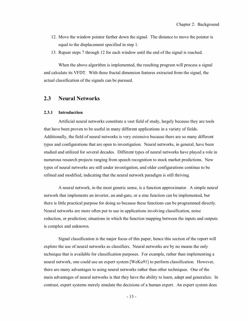
12. Move the window pointer farther down the signal. The distance to move the pointer is
equal to the displacement specified in step 1.
13. Repeat steps 7 through 12 for each window until the end of the signal is reached.
When the above algorithm is implemented, the resulting program will process a signal
and calculate its VFDT. With these fractal dimension features extracted from the signal, the
actual classification of the signals can be pursued.
2.3 Neural Networks
2.3.1 Introduction
Artificial neural networks constitute a vast field of study, largely because they are tools
that have been proven to be useful in many different applications in a variety of fields.
Additionally, the field of neural networks is very extensive because there are so many different
types and configurations that are open to investigation. Neural networks, in general, have been
studied and utilized for several decades. Different types of neural networks have played a role in
numerous research projects ranging from speech recognition to stock market predictions. New
types of neural networks are still under investigation, and older configurations continue to be
refined and modified, indicating that the neural network paradigm is still thriving.
A neural network, in the most generic sense, is a function approximator. A simple neural
network that implements an inverter, an and-gate, or a sine function can be implemented, but
there is little practical purpose for doing so because these functions can be programmed directly.
Neural networks are more often put to use in applications involving classification, noise
reduction, or prediction; situations in which the function mapping between the inputs and outputs
is complex and unknown.
Signal classification is the major focus of this paper, hence this section of the report will
explore the use of neural networks as classifiers. Neural networks are by no means the only
technique that is available for classification purposes. For example, rather than implementing a
neural network, one could use an expert system [WeKu91] to perform classification. However,
there are many advantages to using neural networks rather than other techniques. One of the
main advantages of neural networks is that they have the ability to learn, adapt and generalize. In
contrast, expert systems merely emulate the decisions of a human expert. An expert system does

Chapter 2: Background
- 14 -
not have the ability to adapt or learn, and as a result, its performance is limited by the knowledge
of the expert who designs it. Since a neural network can learn and generalize, it can surpass the
abilities of the experts who created it, and potentially, uncover information that eluded the
experts.
The information presented in this thesis will introduce the basic global concepts behind
the general class of multilayer feedforward neural networks. Once these broad concepts have
been introduced, the main types of neural networks considered in this thesis, namely
backpropagation, complex domain, and probabilistic neural networks, as well as Kohonen self-
organizing feature maps, will be highlighted and explained.
2.3.2 Basic Concepts
The first concept to be mentioned is the general topology of multilayer feedforward
neural networks. Neural networks consist of two main components: neurons and synapses, as
can be seen in Fig. 2.3.
The neurons of a neural network are the units responsible for performing the calculations.
Although the calculations performed by each neuron are relatively simple, when combined with
the calculations of all the other neurons, the neural network as a whole can solve very
sophisticated and complex problems. Neural networks accomplish their goal by passing
messages from neuron to neuron through synapses. The synapses are simply the connections
between neurons and typically have weights associated with them. These weights are adjusted so
that the neural network computes the function that it is supposed to approximate. However, the
inclusion of weights on the synapses is not mandatory. Some neural networks, such as the
Fig. 2.3: A multilayer feedforward neural network.

Chapter 2: Background
- 15 -
probabilistic neural network, define their functionality using other methods which will be
discussed later in this report. Fig. 2.3 further demonstrates that neural networks have inputs and
outputs to interact with the outside world.
An additional observation concerning the neural network shown in the above figure is
that it is organized into several layers of neurons. This aspect of grouping neurons into one or
more layers is a main characteristic of multilayer feedforward neural networks. Multilayer
feedforward neural networks have three or more layers: an input layer, an output layer, and one
or more hidden layers. Typically, the neurons in each layer have different jobs to perform. In
Fig. 2.3, the three neurons on the extreme left make up the first layer, the input layer, of the
neural network. The two neurons in the middle of the diagram form the second layer of the
neural network, the hidden layer. Finally, the remaining two neurons, located on the extreme
right, constitute the output layer. It should also be noted that information in the network
progressively flows from one neuron layer to the next, meaning that the output synapses from
neurons in a particular layer do not connect to neurons in the same or previous layers.
Given the general characteristics and architecture of a multilayer feedforward neural
network, the first operational detail that will be addressed is the manner in which the neurons
operate. The following description applies primarily to the multilayer feedforward class of neural
networks, and it is not applicable to some more specialized types of neural networks, such as
probabilistic neural networks. Despite the lack of universality with the following description, it
will provide insight into the specifics as to how the neurons in a multilayered feedforward neural
network operate. The operational details of the neurons in other neural networks are not
significantly different from the ideas presented here.
The operation of the input neurons is quite simple. The input neurons are merely used for
distribution purposes as their task is to take the inputs that are supplied to the neural network and
distribute them to each of the hidden neurons.
As can be seen from Fig. 2.3, the hidden neurons have one or more input and output
synapses. Fig. 2.4 shows how a hidden neuron processes the signals it receives via its input
synapses, and the procedure through which it generates an output. In the figure, xi represents an
input value along a synapse and wi is the corresponding synaptic weight. The neuron first
multiplies each input by the weight of the synapse on which it is traveling and then sums these
weighted inputs. It should be noted that Fig. 2.4 includes an additional bias input for the neuron.

Chapter 2: Background
- 16 -
Unlike the other synapses, which connect the neurons together, the bias input does not originate
from another neuron. The bias input is simply an additional input to the neuron that always has
an input value of one. The bias input behaves just like any other input in that the weight of the
synapse, wn, multiplied by the input value for that synapse, one, is added to the sum. This
weighted net sum is abbreviated in the equation as net. The f(net) located inside the neuron of
Fig. 2.4 is the neuron’s activation function, which is used to transform the multiple inputs into the
neuron into a single output. The output of the neuron is simply the result of the activation
function upon the net sum:
1
( ) ( )n
i i ni
Output f net f x w w=
= = +∑ (2.10)
The activation function used by the hidden neurons depends on the application, but most neural
networks use a sigmoid activation function. Sigmoid activation functions are smooth,
continuous, monotonically increasing, and are “S-shaped”. There are a variety of different
sigmoid activation functions that can be used with a neural network, but the particular function
chosen typically has little effect on the overall performance of the network. A common sigmoid
function to use is the logistic function, which has the following formula:
1( )
1 xf xe−=
+ (2.11)
Other common sigmoid activation functions include the hyperbolic tangent and arctangent
functions [Mast93].
Usually the output neurons of the multilayer feedforward neural network are designed to
behave in exactly the same fashion as the hidden neurons, but this is not a requirement.
Fig. 2.4: The basic operation of a neuron.
Chapter 2: Background
- 17 -
Up to this point, a description of the topology of multilayer feedforward neural networks
has been presented, and the general operation of the different types of neurons explained.
However, the matter of how the overall neural network is configured to achieve its overall desired
function has not been addressed, and such an explanation is now in order.
One of the main advantages of neural networks, as mentioned previously, is that they
have the ability to learn and generalize. The operational description of the different neurons
certainly has not substantiated these claims. The reason that neural networks have looked so
bland up until this point is that only the execution of a multilayer feedforward network has been
described. That is, the only events that have been detailed so far are the steps involved in
generating an output when a trained network is presented with an input. The real learning
involved with neural networks does not take place when the network is executed, but rather when
the network is trained.
There are two main categories of algorithms that can be used to train a neural network:
supervised and unsupervised training algorithms. With supervised training, the neural network is
provided with both input values as well as the desired output that is associated with each input.
In contrast, unsupervised neural network training involves providing the neural network with just
a set of inputs, but not outputs. In both supervised and unsupervised learning, the basic concept
of training involves optimizing a particular parameter, or set of parameters, throughout the neural
network. For example, in the general multilayer feedforward neural network, training involves
finding an acceptable set of synapse weights so that the neural network can produce the correct
output for any given input.
When training a multilayer feedforward neural network, whether it be supervised or
unsupervised, sample inputs are provided to the neural network After analyzing the outputs that
are produced by the neural network, the parameters being optimized are updated. Each repetition
of presenting the neural network with one or more inputs and adjusting the parameters is known
as an epoch. The number of input presentations that are used to train the network during each
epoch is known as the epoch size. There are some heuristics [Mast93] which outline the epoch
size and the number of epochs that a neural network requires in order to be trained, but the
general idea is to repeat the training process until the error reaches an acceptable level. The exact
manner in which the various parameters are updated during an epoch is different for each type of

Chapter 2: Background
- 18 -
neural network, and thus will be discussed as the different types of neural networks are
introduced.
When solving any practical problem, it is not feasible to train the neural network with
every possible input combination. In fact, in most instances, the entire set of all possible inputs is
not known. Instead, the designer has a set of sample inputs for which he or she knows the correct
output. This set of samples is known as the training set. Choosing an effective training set is
often a challenging problem, as one wants the training set be representative of the entire set of
possible inputs, but the number of known samples from which to select the training set is often
not very large.
Once a neural network is trained, it is almost always necessary to monitor how well the
network performs. In order to gauge the performance of the neural network, a second set of
inputs, known as a testing set, must be selected from the sample inputs. The testing set is
presented to the neural network after it has been completely trained, and the performance of the
neural network is measured by calculating the percentage of the testing set for which the neural
network provides the correct output.
As seen in Fig. 2.5, the testing and training sets must not overlap. The reason for having
testing and training sets completely separated involves the notions of memorization and
generalization. It is relatively easy to train a neural network that is capable of memorizing the
correct responses for each input in the training set. If a neural network is evaluated by using a
testing set that is identical to the training set, it should perform with 100% accuracy. However,
this “test” does not prove anything except the fact that that the neural network was able to
Fig. 2.5: Mutually exclusive training and testing sets.
Known Samples
Training
Set
Testing
Set

Chapter 2: Background
- 19 -
memorize the training set. This performance gauge provides no real indication as to how the
neural network will react if it is presented with an input that it has never seen previously. In any
practical application, the neural network must be able to generalize so that it can produce correct
outputs for inputs that have not been introduced to it during training. Thus, in order to achieve an
accurate measure of generalization and a true unbiased gauge of performance, the testing and
training sets must be mutually exclusive of one another.
This concludes the introduction to the fundamental ideas behind neural networks.
Although the main concepts behind multilayer feedforward neural networks were explained, there
are still many other details that have to be dealt with when designing a neural network. The
answers to these design problems are not trivial and vary from application to application. Even
decisions such as selecting the number of hidden neurons and the number of hidden layers
[Mast93] can be difficult. There are numerous heuristics that can be used in order to determine
near-optimal values for these parameters, but these heuristics are many and varied. Their
intricacies will not be further elaborated upon at this time, but the reasons for making all design
decisions and the ramifications of these decisions will be detailed later in the thesis.
2.3.3 Backpropagation
The backpropagation algorithm is the most common and basic method of training the
general class of multilayer feedforward neural networks. One of the reasons the backpropagation
algorithm is used so frequently is that it is fairly simple. The downside to the backpropagation
training algorithm’s simplicity is that it is slow. Another disadvantage of backpropagation is that
it often has problems dealing with local minima. Despite these shortcomings, the
backpropagation training algorithm has a proven record of providing decent results in practice,
and as such, is taken into consideration in this thesis. Furthermore, the backpropagation
algorithm provides the foundation for training the more advanced complex domain neural
networks, described later in this thesis. This section will provide the concepts and formulas
required for understanding the operation of the backpropagation training algorithm. Full
derivations of the mathematics behind the backpropagation training algorithm can be found in
many neural network texts [Hayk99].
The backpropagation algorithm is a supervised form of training that is used to determine
acceptable values for the synapse weights in a multilayer feedforward neural network. The basic
premise behind backpropagation is as follows. First, the neural network calculates the output for
Chapter 2: Background
- 20 -
an input training vector. Since backpropagation uses supervised training, the output produced by
the network can be compared against the output that is desired for that particular training vector.
More often than not, the desired response and the actual response will not be identical. In other
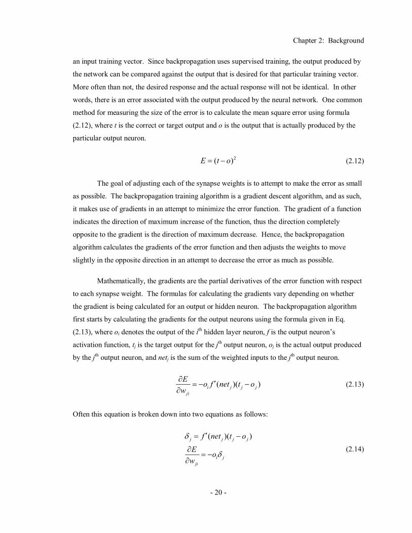
words, there is an error associated with the output produced by the neural network. One common
method for measuring the size of the error is to calculate the mean square error using formula
(2.12), where t is the correct or target output and o is the output that is actually produced by the
particular output neuron.
2( )E t o= − (2.12)
The goal of adjusting each of the synapse weights is to attempt to make the error as small
as possible. The backpropagation training algorithm is a gradient descent algorithm, and as such,
it makes use of gradients in an attempt to minimize the error function. The gradient of a function
indicates the direction of maximum increase of the function, thus the direction completely
opposite to the gradient is the direction of maximum decrease. Hence, the backpropagation
algorithm calculates the gradients of the error function and then adjusts the weights to move
slightly in the opposite direction in an attempt to decrease the error as much as possible.
Mathematically, the gradients are the partial derivatives of the error function with respect
to each synapse weight. The formulas for calculating the gradients vary depending on whether
the gradient is being calculated for an output or hidden neuron. The backpropagation algorithm
first starts by calculating the gradients for the output neurons using the formula given in Eq.
(2.13), where oi denotes the output of the ith hidden layer neuron, f is the output neuron’s
activation function, tj is the target output for the jth output neuron, oj is the actual output produced
by the jth output neuron, and netj is the sum of the weighted inputs to the jth output neuron.
( )( )i j j jji
E o f net t ow∂ ′= − −∂
(2.13)
Often this equation is broken down into two equations as follows:
( )( )j j j j
i jji
f net t o
E ow
δ
δ
′= −
∂= −
∂ (2.14)
Chapter 2: Background
- 21 -
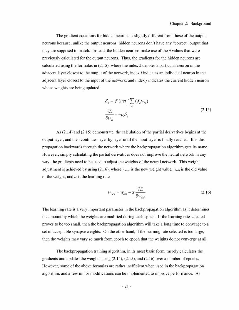
The gradient equations for hidden neurons is slightly different from those of the output
neurons because, unlike the output neurons, hidden neurons don’t have any “correct” output that
they are supposed to match. Instead, the hidden neurons make use of the δ values that were
previously calculated for the output neurons. Thus, the gradients for the hidden neurons are
calculated using the formulas in (2.15), where the index k denotes a particular neuron in the
adjacent layer closest to the output of the network, index i indicates an individual neuron in the
adjacent layer closest to the input of the network, and index j indicates the current hidden neuron
whose weights are being updated.
( ) ( )j j k kjk
i jji
f net w
E ow
δ δ
δ
′=
∂= −
∂
∑ (2.15)
As (2.14) and (2.15) demonstrate, the calculation of the partial derivatives begins at the
output layer, and then continues layer by layer until the input layer is finally reached. It is this
propagation backwards through the network where the backpropagation algorithm gets its name.
However, simply calculating the partial derivatives does not improve the neural network in any
way; the gradients need to be used to adjust the weights of the neural network. This weight
adjustment is achieved by using (2.16), where wnew is the new weight value, wold is the old value
of the weight, and α is the learning rate.
new oldold
Ew ww
α ∂= −
∂ (2.16)
The learning rate is a very important parameter in the backpropagation algorithm as it determines
the amount by which the weights are modified during each epoch. If the learning rate selected
proves to be too small, then the backpropagation algorithm will take a long time to converge to a
set of acceptable synapse weights. On the other hand, if the learning rate selected is too large,
then the weights may vary so much from epoch to epoch that the weights do not converge at all.
The backpropagation training algorithm, in its most basic form, merely calculates the
gradients and updates the weights using (2.14), (2.15), and (2.16) over a number of epochs.
However, some of the above formulas are rather inefficient when used in the backpropagation
algorithm, and a few minor modifications can be implemented to improve performance. As
Chapter 2: Background
- 22 -
mentioned previously, the weights of the neural network are adjusted in the direction which will
result in the maximum decrease in error. This approach is reasonable, but at times it can cause
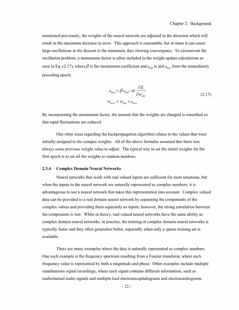
large oscillations in the descent to the minimum, thus slowing convergence. To circumvent the
oscillation problem, a momentum factor is often included in the weight update calculations as
seen in Eq. (2.17), whereβ is the momentum coefficient and old is just new from the immediately
preceding epoch.
new oldold
new old new
Ew
w w
β α ∂= −
∂
= + (2.17)
By incorporating the momentum factor, the amount that the weights are changed is smoothed so
that rapid fluctuations are reduced.
One other issue regarding the backpropagation algorithm relates to the values that were
initially assigned to the synapse weights. All of the above formulas assumed that there was
always some previous weight value to adjust. The typical way to set the initial weights for the
first epoch is to set all the weights to random numbers.
2.3.4 Complex Domain Neural Networks
Neural networks that work with real valued inputs are sufficient for most situations, but
when the inputs to the neural network are naturally represented as complex numbers, it is
advantageous to use a neural network that takes this representation into account. Complex valued
data can be provided to a real domain neural network by separating the components of the
complex values and providing them separately as inputs; however, the strong correlation between
the components is lost. While in theory, real valued neural networks have the same ability as
complex domain neural networks, in practise, the training of complex domain neural networks is
typically faster and they often generalize better, especially when only a sparse training set is
available.
There are many examples where the data is naturally represented as complex numbers.
One such example is the frequency spectrum resulting from a Fourier transform, where each
frequency value is represented by both a magnitude and phase. Other examples include multiple
simultaneous signal recordings, where each signal contains different information, such as
multichannel audio signals and multiple lead electroencephalograms and electrocardiograms.
Chapter 2: Background
- 23 -
The fish trajectory signals used in this thesis, consists of a three dimensional trajectory of a fish,
whereby each sample in the signal can be considered as consisting of three values, one for each of
the Cartesian co-ordinate axes. By restricting the classification to a single plane, complex valued
signals can be obtained by utilizing the samples from one of the axes as the real part of the
samples and the samples from the other axis as the imaginary part.
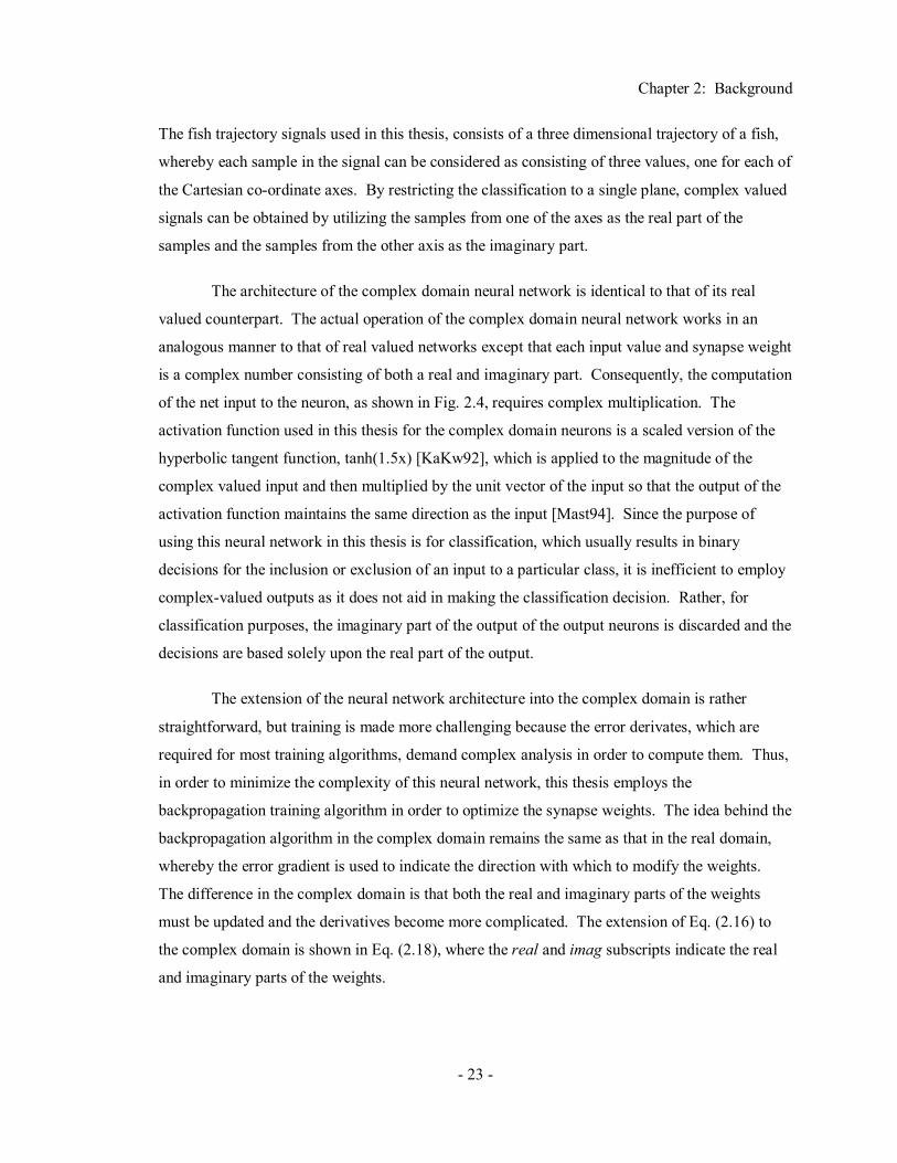
The architecture of the complex domain neural network is identical to that of its real
valued counterpart. The actual operation of the complex domain neural network works in an
analogous manner to that of real valued networks except that each input value and synapse weight
is a complex number consisting of both a real and imaginary part. Consequently, the computation
of the net input to the neuron, as shown in Fig. 2.4, requires complex multiplication. The
activation function used in this thesis for the complex domain neurons is a scaled version of the
hyperbolic tangent function, tanh(1.5x) [KaKw92], which is applied to the magnitude of the
complex valued input and then multiplied by the unit vector of the input so that the output of the
activation function maintains the same direction as the input [Mast94]. Since the purpose of
using this neural network in this thesis is for classification, which usually results in binary
decisions for the inclusion or exclusion of an input to a particular class, it is inefficient to employ
complex-valued outputs as it does not aid in making the classification decision. Rather, for
classification purposes, the imaginary part of the output of the output neurons is discarded and the
decisions are based solely upon the real part of the output.
The extension of the neural network architecture into the complex domain is rather
straightforward, but training is made more challenging because the error derivates, which are
required for most training algorithms, demand complex analysis in order to compute them. Thus,
in order to minimize the complexity of this neural network, this thesis employs the
backpropagation training algorithm in order to optimize the synapse weights. The idea behind the
backpropagation algorithm in the complex domain remains the same as that in the real domain,
whereby the error gradient is used to indicate the direction with which to modify the weights.
The difference in the complex domain is that both the real and imaginary parts of the weights
must be updated and the derivatives become more complicated. The extension of Eq. (2.16) to
the complex domain is shown in Eq. (2.18), where the real and imag subscripts indicate the real
and imaginary parts of the weights.

Chapter 2: Background
- 24 -
real real
real
imag imag
imag
new oldold
new oldold
Ew ww
Ew ww
α
α
∂= −
∂
∂= −
∂
(2.18)
The full derivation of the error gradients shown on the far right of (2.18) will not be developed
here, but the reader is encouraged to read the full derivation in [Mast94].
2.3.5 Probabilistic Neural Networks
This section of the paper will focus on another neural network called the probabilistic
neural network (PNN). Unlike multilayer feedforward networks employing the backpropagation
algorithm, PNNs are based on sound mathematics. Meisel [Meis72] first introduced the basic
mathematical concepts behind PNNs thirty years ago. At that time, Meisel’s ideas seemed to
have very little practical value because the processing of the equations he derived requires a fairly
substantial amount of memory. Today, memory in computers is economic and plentiful, so the
main disadvantage to Meisel’s work has been removed. As a result, the use of PNNs has started
to see some resurgence.
Even though interest in PNNs has recently begun to increase, it is rather surprising, given
the PNN’s numerous advantages, that more research and development has not been performed
using PNNs. One major advantage of PNNs that should attract people’s attention is the fact that
the training time is very fast. In fact, PNNs are able to train several orders of magnitude more
quickly than neural networks using backpropagation training [Wass93]. Another significant
advantage of probabilistic neural networks is the fact that, when used as classifiers, their
classification accuracy asymptotically approaches Bayes optimal [Wass93]. Furthermore, PNNs
do not have nearly as many problems as other neural networks regarding local minima. One
final, practical advantage of PNNs is that training samples can be added or removed without
extensive retraining of the neural network. This compares very favourably to neural networks
based on backpropagation training, which may require that the entire network be retrained when
training samples are added or removed, a very time consuming process.
Of course, if that were all to be said about PNNs, then they would undoubtedly be the
most popular form of neural network in use today. Unfortunately, there are a few disadvantages
with the use of PNNs. The first drawback with PNNs is the fact that they are not as general as
many other types of neural networks. PNNs are predominately designed for classification

Chapter 2: Background
- 25 -
purposes. They can be forced into performing other tasks, but the original intent of PNNs was
classification. Two more difficulties with PNNs are that they are slower to execute than most
other neural networks, and as previously stated, they require a large amount of memory.
The advantages of PNNs definitely appear to outweigh the disadvantages, especially
when the task of the neural network is to perform classification. The potential for PNNs to
approach a Bayes optimal decision indicates that very high classification rates can be attained by
a PNN if it is designed properly. Because of this substantial classification potential, PNNs will be
discussed thoroughly in this thesis.
As a means of introduction, the mathematical concepts behind PNNs will first be
introduced, followed by a description of how these ideas can be molded into the framework of a
multilayer feedforward neural network. The first concept that requires introduction is the Bayes
optimal decision rule and how it pertains to classification. Consider a case in which there are a
number of objects known to be derived from a number of different classes. Simply put, the goal
of a classifier is to identify what class a new, unidentified object belongs to. The Bayes optimal
decision rule for determining which class an unidentified object should be assigned to, is
expressed as follows, in which the object is assigned to class i provided that:
( ) ( ),i i i j j jh c f X h c f X j i> ≠ (2.19)
where hn is the prior probability that new object belongs to class n, cn is the cost of misclassifying
an object that belongs to class n, and fn is the probability density function (PDF) of class n. It
must also be noted that X is the input vector that will be classified. Typically, when dealing with
PNNs the prior probabilities and cost of misclassification are not known a priori and are made to
be equal, hence Bayes optimal decision rule reduces to:
( ) ( ),i jf X f X j i> ≠ (2.20)
This rule indicates that if the PDFs of the different classes are known, then the best classification
decision can be made by merely making a few simple comparisons. Unfortunately, the
probability distributions of the different classes are not usually known and are much too
complicated to attempt to approximate with simpler distributions.

Chapter 2: Background
- 26 -
In order to circumvent the problem of unknown probability distributions, Parzen [Parz62]
introduced a method for approximating the PDFs of each class by using training samples from
each of the classes. Mathematically, the PDF for a single class can be approximated using Eq.
(2.21), where σ is a smoothing parameter, W is the weighting function, X is the unknown input
sample to be classified, Xik is the kth training input from the ith class, n is the number of training
inputs for class i, and gi(x) is the PDF estimate for class i.
1
1( )in
iki
ki
X Xg X Wnσ σ=
− =
∑ (2.21)
As the number of sample inputs, n, for class i increases, Eq. (2.21) approaches the true PDF for
class i. When all of the PDF estimations are calculated, they are used in Eq. (2.20) in place of the
true PDFs and the classification decision is made.
There are still two facets of (2.21) that require further explanation: the weighting
function, W, and the scaling parameter, sigma, σ. For estimating the PDFs, a weighting function
is needed so that when the unknown sample to be classified is in close proximity to a particular
training sample (i.e. the input to the weighting function is small), the weighting function produces
a large value. In other words, when the unknown sample is quite similar to one of the training
samples from a particular class, the value of the estimated PDF for that class should increase
rather substantially. On the other hand, if the unknown sample and an input training vector are
not very close to one another (i.e. the input to the weighting function is large), the weighting
function should produce a small value. In this case, the unknown input is quite different from the
training sample from the particular class, and as such, the PDF for that class should not be
increased much at all. Typically, the proximity or distance between the training sample and the
unknown input is measured using Euclidean distance. The weighting function often used is the
Gaussian function because it exhibits the aforementioned properties and is relatively easy to
calculate. By setting the weighting function to the Gaussian function, (2.21) becomes:
2
2/ 2
1
21( )(2 )
iikn
i p pki
X X
g Xσ n
e σπ =
−−
= ∑ (2.22)
where p is the length of the input vector, X.

Chapter 2: Background
- 27 -
The second aspect of the PNN formulas that still requires clarification is the role of the
scaling parameter, sigma. The scaling parameter dictates how wide an area the weighting
function takes into account when determining the contributions of each training sample. If sigma
is selected to be too small, then only those training samples that are extremely close to the
unknown input will have any major contribution to the estimated PDFs. As a result, the
classification system simply breaks down to a nearest neighbour classifier. If, however, the
sigma selected is too large, then even training samples that are separated by a great distance from
the unknown input will have a large contribution to the estimated PDFs, causing the system to
display matched filter behaviour. Hence, some effort must be put forth to find an appropriate
scaling parameter for the particular classification problem. Fortunately, in most problems, there
is a range of values that will yield acceptable results [Wass93][Spec88], as can be seen in Fig.
2.6. Hence, since there is typically a plateau of sigma values producing optimal results,
extremely intense algorithms do not have to be utilized to find an exact, superior sigma value.
It should also be mentioned at this point that multiple sigma values can be employed
when using a PNN. For example, different sigma values can be utilized for each of the different
classes. Separate sigma values for each class can be useful if some classes are very tightly
defined (the training samples from such classes are very similar to one another) while other
classes are more loosely defined (the training samples from such classes vary over a wider range).
The idea of using different sigma values for each class is considered in this thesis. The formula
for calculating the PDFs for such a multi-sigma PNN is almost identical to Eq. (2.22) and is given
in (2.23).
Fig. 2.6: Correct classification rate as a function of sigma,σ.
Cor
rect
Cla
ssifi
catio
ns Optimum
Nearest Neighbour
Matched Filter
Sigma, σ

Chapter 2: Background
- 28 -
2
2
/ 21
21( )(2 )
iik
ni
i p pki i
X X
g Xσ n
e σ
π =
−−
= ∑ (2.23)
The only difference between equations (2.22) and (2.23) is the presence of the subscript i for each
sigma, indicating its class membership.
Now that the mathematics behind the PNN have been described, the manner in which the
math is mapped to the architecture of a multilayer feedforward network, as first performed by
Specht [Spec88], will briefly be explained. The architecture of a PNN is organized into four
layers: the input layer, pattern layer, summation layer, and output layer, as seen in Fig. 2.7.
The role of the input layer in the PNN is virtually identical to that of the other neural
networks described thus far. In essence, the input layer accepts input values from the outside
world and then distributes those inputs to each of the neurons in the pattern layer. No
computations are performed. Each neuron in the pattern layer corresponds to a training sample of
the PNN. Notice that for Fig. 2.7, the neurons in the pattern layer have been grouped into three
sets representing three different classes. The job of each pattern layer neuron is to compute the
Fig. 2.7: Basic architecture of a PNN.
Input
Layer
Pattern
Layer Summation
Layer
Output
Layer
Chapter 2: Background
- 29 -
result of the weighting function.
The summation layer neurons have a different task to fulfill than that of the pattern layer
neurons. There is a single summation layer neuron for each class. A summation layer neuron
accepts the result of the weighting functions for each training vector belonging to its class, and
then calculates the sum. In essence, the summation layer is performing the summation as seen in
(2.22) and (2.23).
Generally, there is only one neuron in the output layer in the basic PNN. The output
neuron accepts all the results from each of the summation neurons and selects the class that
generates the largest sum.
2.3.5.1 Probabilistic Neural Network Training
Now that the mathematics behind PNNs and the method by which those mathematical
functions are formed into a neural network architecture have been explained, the next topic that
must be discussed is the process of training a PNN. As indicated earlier, the scaling parameter,
sigma, must be optimized such that it matches the cluster sizes of the different classes. To
perform this optimization, a two step line minimization algorithm is used [Mast95]. Specifically,
the minimum must first be bounded, and then a search over the bounded interval is performed to
find the actual minimum.
At its roots, single sigma optimization is merely a single variable optimization problem.
Optimization problems are typically easily resolved provided the function one is attempting to
optimize is known. The process of differentiating the function and setting the result to zero yields
the function’s minima and maxima. However, in the case of optimizing sigma, the exact
description of the function is not known. As a result, other means of optimizing sigma must be
used. The only way to definitively find the globally optimal sigma value is to search the entire
problem space. However, this is obviously not a practical solution, as it would require an infinite
amount of time.
As mentioned, the line minimization algorithm used in this thesis for optimizing sigma
begins by attempting to bound the minimum. This process entails the selection of several trial
sigma values within a given range, and then evaluating each trial sigma to observe how it
performs. When complete, the algorithm returns three sigma values. The middle sigma produces
the best results out of the trial sigma values. The first and third sigma values returned are the trial

Chapter 2: Background
- 30 -
points to the immediate left and right of the middle sigma value. Obviously the first and third
values returned do not perform as well as the middle value. Hence, there must be a minimum in
this interval defined by the three sigma values. The minimum in this interval may not be the
absolute global minimum, but it is assumed that it will provide adequate performance.
The bounded interval defined by the three sigma values found in the first stage can be
quite large, but the second step of the line minimization will usually locate the minimum after
completion of a small number of trial points. The algorithm used for the second step of the line
minimization process utilizes a sectioning algorithm in an attempt to minimize the number of trial
sigma values required to locate the minimum. This portion of the line minimization algorithm
begins with the best sigma produced in the bounding stage. The algorithm compares the distance
between the current minimum sigma value and its left neighbour, as well as the current minimum
sigma value and its right neighbour. The algorithm selects the larger of the two intervals in order
to search for a better minimum. The value of the new trial sigma, located in the larger of the two
intervals, is dictated by the particular sectioning algorithm used. In bisectioning, the most
intuitive case, the trial sigma is the point in the middle of the interval; of course, the interval
could be sectioned in any number of other ways. If the trial sigma produces a better result than
the current best sigma, then the optimal sigma and its bounds are updated. On the other hand, if
the trial sigma does not outperform the current best sigma, the optimal sigma remains the same,
but the bounding points are altered to narrow the search interval. This process is repeated until it
is determined that the current optimal sigma produces sufficiently accurate results, or the bounded
interval gets so small that new trial sigma points are only slightly different from the current best
sigma.
The above line minimization algorithm is by no means the most sophisticated method for
finding a near-optimal sigma value. There are many more complex methods, such as genetic
algorithms and simulated annealing, that could be utilized for this optimization step, but the two
step line minimization algorithm presented here is much faster than most other algorithms, and
still is very effective. As Fig. 2.6 indicates, there is usually a range of acceptable sigma values,
hence this simple optimization algorithm will often produce sufficient results in a fraction of the
processing time.
One matter that has yet to be mentioned is the manner by which the validity of a sigma
value is determined. The procedure outlined here for evaluating the performance of a particular

Chapter 2: Background
- 31 -
sigma is called jackknifing [Mast93]. Jackknifing is a reliable method for evaluating different
sigma values because it provides a very good representation of how well a particular sigma
performs, while at the same time does not require an excessive number of training samples.
When training the PNN, several known input samples are used to serve as examples from
each of the different classes. These known examples are the network’s training set. The premise
behind jackknifing is to train and test the PNN k times, where k represents the number of training
data samples. During each of the k trainings sessions, one of the training sample inputs will not
be included in the training process. Then, once the PNN has been trained, the single training
vector that was excluded will be presented to the PNN to be classified. During each of the k
training and testing sessions, should the single excluded training input be incorrectly classified,
the sigma value receives a point. The lower the score a sigma receives the better, as the score
indicates the total number of inputs the PNN has incorrectly classified.
The jackknifing metric provides a reasonable measure of performance for a particular
sigma value when the goal is to try to optimize sigma. However, it must be stressed that
jackknifing is a biased measure of performance because the testing inputs are being used to train
the neural network. As a result, the true ability of the PNN should be measured once training has
been completed. This measurement would be performed by attempting to classify a testing set
which does not include samples that were present in the training set.
A few points should be mentioned about the manner of optimizing sigma values when a
different sigma is used for each of the different classes. In this scenario, the problem has been
extended to a multivariate optimization problem, and as such, is slightly more difficult. The
technique utilized in this thesis to determine an acceptable set of sigma values is a conjugate
gradient method. As conjugate gradient methods are standard mathematical entities, a full
description will not be provided here, but there are many reference materials available that
describe such algorithms in full detail [PrFTV88].
One requirement for the conjugate gradient algorithm that must be discussed is that of a
continuous error function. When performing single sigma optimization, the jackknifing
technique measures the performance of a particular sigma value based on a point scoring system.
The fewer the number of points a sigma value receives, the better it has performed in its
classification, since the points signify errors. This technique is sufficient for the single sigma
optimization, but something more sophisticated must be used for multi-sigma training.

Chapter 2: Background
- 32 -
Specifically, a continuous error function must be derived whereby the goal of the conjugate
gradient algorithm is to minimize the error function. There are two main reasons why a
continuous error criterion is used for the conjugate gradient algorithm rather than the point
scoring system. First, a continuous error function provides the jackknifing algorithm with a
superior metric as to how well a set of sigma values performs. With the point scoring system
described for single sigma training, tied results would occur quite frequently, whereas with a
continuous error function the occurrence of ties is much more of a remote possibility. The
second, more important reason for selecting the continuous error function is that the conjugate
gradient algorithm uses the error function and its partial derivatives with respect to the sigma
values in order to perform its optimization.
The continuous error criteria used for this project is defined in (2.24), where X is the
input being classified, index i is the class to which X belongs, index k represents all of the other
classes, and bn are the Bayesian confidences.
[ ] [ ]2 2( ) 1 ( ) ( )i i kk i
e X b X b X≠
= − +∑ (2.24)
The Bayesian confidences, are defined in (2.25), where K is the number of classes and gi(X) is
defined in (2.23).
1
( )( )( )
ii K
ik
g Xb Xg X
=
=
∑ (2.25)
Equation (2.24) intuitively seems reasonable because if X belongs to class i, then ideally the
Bayesian confidence, bi, will be close to 1, and bk, k ≠ i, will be close to 0, which will produce a
small error. If bi decreases, an indication that the PNN did not believe X belonged to class i (an
incorrect result), then the error produced will be larger.
The full derivation of (2.24) and its first and second partial derivatives with respect to the
sigma values will not be presented here as they become quite tedious, and are not a core
component to understanding the thesis as a whole. Hence, for further information regarding the
continuous error function and its derivatives that are used in conjunction with the conjugate
gradient function, the reader is encouraged to refer to [Mast95].

Chapter 2: Background
- 33 -
2.3.6 Kohonen Self-Organizing Feature Maps
Kohonen self-organizing feature maps (SOFMs) are neural networks that use
unsupervised competitive learning algorithms. These neural networks are referred to as topology-
preserving in that the neighbourhood relations of the data are preserved and structure is imposed
upon the neurons in the network [Koho84]. This clustering of the data based on their relations
allows for the discovery of the underlying structure of the data. The use of SOFMs in this thesis
is two-fold. First, SOFMs are incorporated for objectively determining the clusters, or classes, of
the signals used to verify the classification system. The second use of the SOFMs in this thesis is
for feature extraction purposes by creating a signature pattern for a given signal.
An SOFM is composed of just two layers of neurons: an input layer and an output layer.
The neurons in the output layer simply output the Euclidean distance (or the square of the
Euclidean distance) between its weights and the input, as shown in (2.26), where n is the number
of inputs to the network.
2
1
( )n
j ji ii
out w input=
= −∑ (2.26)
The neuron that has the smallest output is declared the “winner”. It is this “winner” that
is allowed to have its weights updated, hence the competitive nature of the learning. Training of
the network is performed by modifying the weights of the “winner” neuron to make it more
closely resemble the input as shown in Eq. (2.27), where w is the neuron weight, index k signifies
the “winner” neuron, and index i is the input neuron.
( )ki ki i kinew old old
k j
w w input w
k out out j k
η= + −
> ∀ ≠ (2.27)
In addition, the surrounding neurons also have their weights updated during training, in
order to encourage groupings and clusterings. It is this group learning from which the SOFM
attains its power. The aim of the training is to have similar inputs activate neurons in the same
area. The function that dictates which nearby neurons also learn is referred to as the
neighbourhood function. There are many different neighbourhood functions that can be used,
such as a constant, linearly decreasing, exponentially decreasing, or Mexican hat, which uses
negative learning rates in an attempt to more distinctly isolate the groupings [EbDo90].

Chapter 2: Background
- 34 -
However, the neighbourhood function has little overall effect on the SOFM as long as enough
training is permitted for the network to converge to a steady state [Fere95]. This thesis uses a
constant neighbourhood function where all neurons within a designated distance, or radius, of the
“winner” neuron have their weights updated at the same rate as the “winner” neuron. A heuristic
is used whereby the radius of the neighbourhood function decreases along with the learning rate
as the training progresses. Using this technique, the SOFM initially roughly defines the clusters
when the radius and learning rate are high and then refines these clusters as training progresses
and the radius and learning rate are decreased.
There are two common ways in which the neurons in the output layer can be organized.
The first is simply in a one-dimensional array, and the second is in a two-dimensional matrix.
The main difference between these layouts is how the neighbourhood function is defined, in that
for the two-dimensional case, there are neighbouring neurons in multiple directions that may have
their weights updated. This thesis does not consider this type of SOFM as the signals used in this
thesis are represented as one-dimensional vectors and do not require the extra complexity of the
two-dimensional SOFM.
The primary manner in which SOFMs are used in this thesis is for feature extraction of
signals. The number of weights in the SOFM is typically less than the length of the signal that is
used to train it. Hence, when the SOFM is presented with segments from the signal, the weights
of the SOFM have to adjust such that they represent the predominant characteristics that are
present in the signal. In other words, the weights are adjusted such that they represent the most
prominent features in the signal. When training is complete, the set of weights contained in the
SOFM are commonly referred to as the codebook, as it contains a set of codes representative of
the signal. These weights, or codes, within the codebook are known as codewords and each
codeword represents a specific feature that the SOFM found within the signals. In addition to the
reduction in the number of features representing the signal, the use of SOFMs provides some
translational robustness in that signals which are mere translations of one another result in very
similar codebooks.
The second way in which SOFMs are used for this thesis is to derive the different classes
from the signals by exploiting the SOFM’s clustering abilities. Clustering algorithms are not the
main focus of this thesis but are utilized to form the training and testing sets for the purpose of

Chapter 2: Background
- 35 -
classification since the annotations of the signals used in this thesis were not provided. A more
thorough discussion of the use of SOFM for clustering can be found in Appendix B.
2.4 Summary
This section of the thesis has provided the background on signal classification and has
introduced the techniques used to perform feature extraction for the purpose of classification,
namely, the variance fractal dimension trajectory and Kohonen self-organizing feature maps. In
addition, the probabilistic and complex domain neural networks have been presented as they are
used to perform the signal classification based on these features.

Chapter 3: System Design
- 36 -
CHAPTER 3
SYSTEM DESIGN
One of the primary goals of the signal classification system is a maximal independence
from the signal itself. It is this requirement that drives much of the design of the architecture of
the system and the components of the system.
There are three main design goals for the classification system developed for this thesis:
the average correct classification rate must be greater than 90%; the time required to train the
system must be less than a day; and the time required for the system to classify a given input
signal must be shorter than the duration of the signal itself. The correct classification rate of 90%
was selected because this success rate indicates that the system is able to correctly classify inputs
with a high degree of consistency. Additionally, a rate of 90% was deemed to be a reasonable
target given the time-constraints of the thesis.
The training time design constraint was selected in a less precise manner because there
are no reasons in this thesis to dictate a definitive time limit for the training of the system. Thus,
the training time criterion was selected so as to ensure that the system was capable of training in a
time frame in the realm of reasonability. As a result, the constraint for the training time of the
classification system was selected to be on the order of minutes or hours, and not days or months.
The final design criteria specifying that the execution of the classification system require
less processing time than the duration of the signal itself was decided to ensure that the system
could be applied to performing analysis on signals in real-time, should it be required.
3.1 System Architecture
There are many challenges for a system flexible enough to work with a variety of
different signals while requiring minimal changes to the system. One of the first issues in such a
system is simply reading the signal from its raw data representation since there is no universally
adopted format with which to represent signals. The first component of the system is
preprocessing, as shown in Fig. 3.1, and the primary function of the component is to convert the
signals from their original data representation to a proprietary format developed for this thesis.
The application of a different signal to the system primarily requires only a minor addition to the

Chapter 3: System Design
- 37 -
preprocessing stage to perform the necessary data conversion. This common data representation
provides the ground from which the rest of the system can stand upon.
The preprocessing stage is also responsible for performing any necessary filtering to
reduce noise or other signal manipulations required before its analysis. For the purpose of this
thesis, no filtering is performed so as to further test the robustness of the system.
The task of designing the part of the system to perform the actual classification of signals
seems daunting at first because of the abundance of signal processing techniques available. The
main idea behind classification is to group the signals into classes in which membership to a
particular class is based solely upon a selected set of features. The entire classification of the
signals is dependent upon the careful selection of the features with which to uniquely identify
each class of signals. The difficulty is that there are an infinite number of features to choose,
ranging from the average value of the samples, the variance of the samples, Fourier transform
coefficients, wavelet coefficients [Mall98], or even the signal samples themselves. For the
signals examined in this thesis, simple statistical measures are insufficient to uniquely identify the
signal classes and the ubiquitous Fourier transform is not applicable because of the non-
Fig. 3.1: System block diagram.

Chapter 3: System Design
- 38 -
stationarity of the signal and the non-linear processes that generate these signals. It is naïve to
simply use the samples from the signal to attempt to identify the classes because in most cases,
this results in too many features for the classifier to base the classification upon. Furthermore, the
sample domain is very sensitive to changes in amplitude, frequency, and phase. The windowed
Fourier transform or wavelet transformation could however be utilized, but this thesis chooses to
take advantage of the self-similarity of the signals and use a multifractal characterization with
which to uniquely identify each class. The particular technique used is to represent the signal as a
trajectory of its variance fractal dimension through sliding windows across the signal. The
advantages of this transformation are two-fold. First, this scale-invariant transformation
emphasizes the underlying complexity of the signal, which provides the unique identification for
each class. Second, the transformation provides a normalizing effect since the theoretical limits
of dimensionality of Euclidean one-dimensional signals is bound between one and two.
Normalization is critical for the classification process, since all signals in a particular class must
have similar values for the defined set of features. Without normalization, signals in the same
class could potentially take on any values for the set of features and it would be impossible to
perform classification because the range of acceptable values would be infinite.
Without any further feature extraction, the classification can be performed based solely
upon the signal’s variance fractal dimension trajectory (VFDT), and this is explored by this
thesis. The difficulty is that the VFDT is actually another signal. Although it is much less
sensitive than the original signal, it still suffers from translational problems. Slightly shifted
VFDTs should be interpreted to be of the same class, but when compared sample by sample, they
would be quite different. Feature extraction upon the VFDT itself could be performed using any
of the techniques mentioned previously, but the goal is to not lose the normalization achieved or
the features already extracted. The technique proposed is the use of Kohonen self-organizing
feature maps (SOFMs). The goal is to extract the characteristic features of the VFDT and form a
fingerprint of it. The SOFM will form a codebook that represents the VFDT and slightly sample
shifted signals would then have very similar codebooks. Furthermore, this feature extraction can
lead to a compression in the number of features used to represent the signal and hence, reduce the
size of the classification problem
With the set of features established, the remaining task is to perform the actual
classification of the signals based on these features. The classification should be automated and
not be specific to the actual signal being classified. There are two main lines of thinking for
Chapter 3: System Design
- 39 -
performing this task: expert systems and machine learning. Expert systems involve establishing
customized predefined rules for separating the signals into classes based on their features;
however, this is too rigid of a structure to be easily adaptable to different signals. Furthermore, in
most cases, it is not known how to arrive at concrete rules about how to perform this
classification.
Machine learning, on the other hand, entails having the computer discover its own way of
performing the classification based on some examples of signals belonging to each class. Simply
providing examples of each class requires much less work than specifically defining the rules
needed to determine exactly how to classify the signals based on the selected features. Utilizing
machine learning allows the data to speak for itself. The particular choice of machine learning
used in this thesis is neural networks. Neural networks are used in this thesis for their ability as
function approximators, meaning that they can learn virtually any function. Additionally, neural
networks were chosen because of their generalization ability and robustness to noise, meaning
that they perform well upon data they have never seen before and in situations involving
abnormalities. This flexibility is important because with any classification, there will be some
variability in the acceptable values of features for a given class.
Even with the decision of utilizing neural networks to perform the classification, there are
a variety of neural networks to choose from. While the basic backpropagation neural network
generally comes to mind, it is not the best neural network to choose for classification. The
probabilistic neural network (PNN), or Bayes classifier, trains faster and is asymptotically
optimal as the number of training vectors increases.
One aspect to consider is that some signals are composed of multiple recordings, each
capturing different information about the physical system. In the case with two simultaneous
signal recordings, the signal can be considered to consist of a single array of samples, each of
which are represented as complex numbers, where the real part is a sample from one of the
recordings and the imaginary part is a sample from the other recording. Extensions to
hypercomplex numbers, where three or more simultaneous recordings are available, are possible,
but this thesis will restrict the number of signals to being complex.
Ignoring the additional information that the multiple recordings provide could restrict the
performance of the classification. The SOFMs can be modified to handle the values as complex
numbers, as can the PNNs by appending the second signal to the first and creating a single real
Chapter 3: System Design
- 40 -
valued signal; this technique is discussed in the corresponding component design sections. As an
alternative to the PNN, this thesis also proposes to use a complex domain neural network to
perform the classification upon the signals and take advantage of this additional information as
well as the strong coupling between the two values that compose each complex valued sample.
This extension to the complex domain adds complexity, so the basic backpropagation training
algorithm is used. It is not known to what extent the inclusion of additional information with the
use of complex domain neural networks will have on the classification, so comparisons will be
made between probabilistic neural networks using one or both fish signal recordings and the
complex domain neural networks using both fish signals simultaneously.
3.2 Component Design
Even with the components selected for use in this thesis, many design decisions must be
made about the components themselves, as there are a variety of options available and several
parameters to set.
3.2.1 Preprocessing
The function performed by this component is to perform data conversion from the raw
data format of the signal to a proprietary format developed for this thesis. For the most part, each
type of signal has its own unique file format, so the data conversion involves parsing any relevant
information from the file header and translating the signal samples from their original ASCII,
binary, or other encoding schemes. Further complicating matters, some raw data files contain
multiple signals, which must be separated in order to facilitate the function of the other
components. Thus, for a given raw data file containing n signals, the output of the preprocessing
stage is n files, each containing one of the signals from the original data file in the proprietary
format used in this thesis.
The format chosen for this thesis is simple but contains all the information needed to
perform the analysis upon it. The processed files representing the signals have some basic header
information containing the sampling rate of the signal and the number of samples in the file. This
header is followed by the actual samples of the signal. All values are written in uncompressed
binary, little endian format, with floating and double point values conforming to the IEEE 154
standard. This file format allows for flexibility in the data type of the sample points, since it is
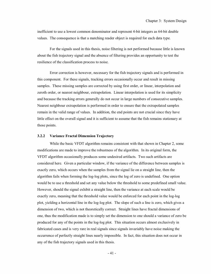
Chapter 3: System Design
- 41 -
inefficient to use a lowest common denominator and represent 4-bit integers as 64-bit double
values. The consequence is that a matching reader object is required for each data type.
For the signals used in this thesis, noise filtering is not performed because little is known
about the fish trajectory signal and the absence of filtering provides an opportunity to test the
resilience of the classification process to noise.
Error correction is however, necessary for the fish trajectory signals and is performed in
this component. For these signals, tracking errors occasionally occur and result in missing
samples. These missing samples are corrected by using first order, or linear, interpolation and
zeroth order, or nearest neighbour, extrapolation. Linear interpolation is used for its simplicity
and because the tracking errors generally do not occur in large numbers of consecutive samples.
Nearest neighbour extrapolation is performed in order to ensure that the extrapolated samples
remain in the valid range of values. In addition, the end points are not crucial since they have
little effect on the overall signal and it is sufficient to assume that the fish remains stationary at
those points.
3.2.2 Variance Fractal Dimension Trajectory
While the basic VFDT algorithm remains consistent with that shown in Chapter 2, some
modifications are made to improve the robustness of the algorithm. In its original form, the
VFDT algorithm occasionally produces some undesired artifacts. Two such artifacts are
considered here. Given a particular window, if the variance of the difference between samples is
exactly zero, which occurs when the samples from the signal lie on a straight line, then the
algorithm fails when forming the log-log plots, since the log of zero is undefined. One option
would be to use a threshold and set any value below the threshold to some predefined small value.
However, should the signal exhibit a straight line, then the variance at each scale would be
exactly zero, meaning that the threshold value would be enforced for each point in the log-log
plot, yielding a horizontal line in the log-log plot. The slope of such a line is zero, which gives a
dimension of two, which is not theoretically correct. Straight lines have fractal dimensions of
one, thus the modification made is to simply set the dimension to one should a variance of zero be
produced for any of the points in the log-log plot. This situation occurs almost exclusively in
fabricated cases and is very rare in real signals since signals invariably have noise making the
occurrence of perfectly straight lines nearly impossible. In fact, this situation does not occur in
any of the fish trajectory signals used in this thesis.
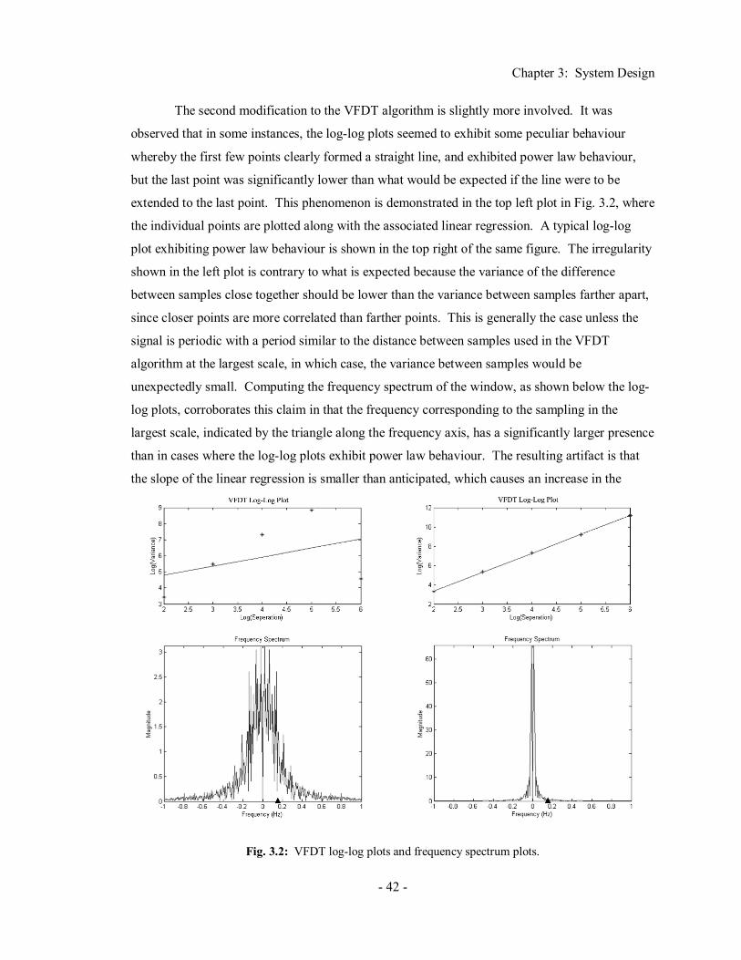
Chapter 3: System Design
- 42 -
The second modification to the VFDT algorithm is slightly more involved. It was
observed that in some instances, the log-log plots seemed to exhibit some peculiar behaviour
whereby the first few points clearly formed a straight line, and exhibited power law behaviour,
but the last point was significantly lower than what would be expected if the line were to be
extended to the last point. This phenomenon is demonstrated in the top left plot in Fig. 3.2, where
the individual points are plotted along with the associated linear regression. A typical log-log
plot exhibiting power law behaviour is shown in the top right of the same figure. The irregularity
shown in the left plot is contrary to what is expected because the variance of the difference
between samples close together should be lower than the variance between samples farther apart,
since closer points are more correlated than farther points. This is generally the case unless the
signal is periodic with a period similar to the distance between samples used in the VFDT
algorithm at the largest scale, in which case, the variance between samples would be
unexpectedly small. Computing the frequency spectrum of the window, as shown below the log-
log plots, corroborates this claim in that the frequency corresponding to the sampling in the
largest scale, indicated by the triangle along the frequency axis, has a significantly larger presence
than in cases where the log-log plots exhibit power law behaviour. The resulting artifact is that
the slope of the linear regression is smaller than anticipated, which causes an increase in the
Fig. 3.2: VFDT log-log plots and frequency spectrum plots.

Chapter 3: System Design
- 43 -
fractal dimension.
To remove these artifacts, the last point is discarded in log-log plots where the points are
progressively increasing in value, but the last point is lower than its predecessor. By ignoring the
last point in these instances, the linear regression can then capture the power law behaviour
exhibited by the remaining points. Periodicities corresponding to the last point is not the only
problem, since periodicities affecting the separation corresponding to the second last point would
have a similar affect. In such a scenario, both the second last point and the last point would be
lower than expected because the frequency corresponding to the last point is merely a harmonic
of the second. More sophisticated algorithms could be used to eliminate the outliers in general,
but are not explored in this thesis since it was observed that artifacts caused by these periodic
situations had a low rate of occurrence.
Aside from the design modifications to the VFDT component itself, there are also design
decisions to be made concerning the two free parameters involved in the algorithm. The choice
of the window size is very important and unfortunately, the choice is specific to each type of
signal. Generally, the window size is chosen to match the stationarity of the signal; however,
since such knowledge does not exist for the fish trajectory signals used in this thesis, the window
is experimentally determined. The window is chosen such that in general, the log-log plots obey
a power law relation. The second parameter is the displacement of the sliding windows. The
amount that the sliding window is shifted for each calculation of a variance fractal dimension
determines the resolution of the VFDT. Unlike the window size, the experimental determination
of the window displacement is more subjective in nature. Furthermore, these two parameters
affect the size of the classification problem in that the value of the window size and displacement
control the number of features to be used for classification. The actual choice of the window size
and displacement used during the verification of the classification system is discussed in the
experimental results and discussion in Chapter 6.
3.2.3 Kohonen Self-Organizing Feature Map
For the purpose of feature extraction and further reduction of the size of the classification
problem, SOFMs are used to produce a fingerprint of the VFDT by picking out the most common
characteristics from the VFDT. The fingerprint produced is simply the codebook of the SOFM
trained using samples from the VFDT signal. For a given codeword length, the SOFM is trained
by providing it with intervals of the VFDT with the same length as the codeword. The SOFM

Chapter 3: System Design
- 44 -
then determines the most representative codewords from the VFDT and arranges them in a
topological-preserving manner. The classification is then based upon these set of codewords.
Because the chosen intervals of the VFDT are allowed to be shifted anywhere along the signal,
the codebooks should be more robust to translational shifting than the VFDT signals. While the
codeword length is important because it determines the size of the features extracted from the
VFDT, the number of codewords is also an important because it determines the number of
features selected. If the number of codewords is too small, then the SOFM cannot capture all the
important features. Conversely, if the number of codewords is too large, then the size of the
classification problem is larger than necessary and the SOFM may extract insignificant features.
These parameters are determined experimentally and their choices specific to the fish trajectory
signals are discussed in Chapter 6.
Another architectural design decision is the organization of the neurons in the SOFM.
The most common organization represents the neurons in a two-dimensional map; however, since
the signals used in this thesis are one-dimensional in the Euclidean sense, and to reduce the
complexity of the SOFMs, the neurons are organized one after another in a one-dimensional
array.
As it is currently presented, the SOFM is only able to form a codebook based upon a
single real valued signal. In order to extend the SOFM such that it can perform feature extraction
of two signals simultaneously in cases where the classification is dependent upon two separate,
but correlated signals, each signal sample can be represented as a complex number, with the real
part representing a sample in one signal, and the imaginary part representing a sample in the other
signal. By replacing the real domain Euclidean distance between the neuron weight and the input
vector in Eq. (2.26) with the more general complex domain version, and performing some
straightforward manipulations, Eq. (3.1) can be obtained.
2
1
n
j ji ii
out w input=
= −∑
2
2 2
1
( ) ( )n
j ji i ji ireal real imag imagi
out w input w input=
= − + − ∑
2 2
1 1
( ) ( )n n
j ji i ji ireal real imag imagi i
out w input w input= =
= − + −∑ ∑ (3.1)

Chapter 3: System Design
- 45 -
This result demonstrates that using an SOFM that accepts complex valued inputs is equivalent to
a real domain SOFM where the real and imaginary parts of the input are concatenated to form a
single real valued array. Thus, no architectural changes are required to have the SOFM perform
feature extraction upon multiple simultaneous signals.
The input to the SOFM are intervals of VFDT signals, consequently, the values are, for
the most part, normalized between one and two, and hence the weights of the SOFM need only be
between one and two. Since no assumptions are made about the signal or its VFDT, the weights
are initialized by simply using random numbers uniformly distributed between one and two.
The training of these initially random weights involves a number of design decisions.
The epoch size is set to one, meaning that the weights are updated after each presentation of a
training vector as that is the standard for this neural network. Since no a priori knowledge about
the VFDT is assumed, the training vectors are randomly selected intervals from a single VFDT
signal. Because the training is unsupervised, there is no right or wrong that can be assessed, so
the number of training vectors presented to the SOFM is fixed and simply such that the SOFM
converges to a steady state. Again, this value is determined experimentally, but in general, each
training vector should be presented at least a couple of times during training. Another decision to
be made is the neighbourhood function to use for training. The neighbourhood function is not
that important as its primary effect is a slight alteration of the speed of convergence of the
network. As such, the simplest function, the constant function, is used where all the neurons
within a particular distance, or radius, of the “winner” neuron learns at the same level. The
choice of the radius of the neighbourhood function and learning rate are however, quite
important. Initially these parameters are set to large values in order to establish the general
groupings in the map and are then decreased as the training proceeds in order to refine the
clustering. The question arises as to how to decrease these parameters. Two disparate options are
exponential and linear reductions of the parameter values. Through experimentation, it was
discovered that exponential reduction does not produce good results because the parameters are
reduced too quickly and the general clustering is not properly established before the parameters
decrease to levels where refinement dominates. As a result, maps are produced where the clusters
and extracted features are poorly defined. Linear reduction causes the SOFMs to converge
quicker and produce better clustered codebooks representative of the training vectors. The initial
radius of the neighbourhood function is set to the size of the codebook and the learning rate is set
Chapter 3: System Design
- 46 -
to 0.9. Both parameters and they are reduced in a linear fashion until the radius is 0, meaning that
no neighbouring neurons are affected, and the learning rate is 0.1.
3.2.4 Probabilistic Neural Network
Probabilistic neural networks (PNNs) are utilized in this thesis for their excellent
classification ability. The majority of the design decisions in regard to the PNN relate to the
smoothing parameter, or sigma value, used in the Gaussian functions in the pattern layer of the
neural network. The first decision to be made is whether a single sigma value is to be used for
each feature. A different sigma may be desired for different features if the features have different
normalizations or importance. For this thesis, the features provided to the PNN are either a
VFDT signal or a SOFM codebook created from a VFDT signal, thus there are no reasons to have
any preference or special consideration for any particular feature, as they all represent fractal
dimensions. However, when the PNN is used to classify complex valued signals consisting of
samples from two separate recordings, things are slightly different. When dealing with complex
valued inputs with the PNN, a transformation is performed whereby a single input to the PNN is
formed by the concatenation of the two recordings, which is identical to how this situation is
handled with the SOFM in Eq. (3.1). Such a transformation is valid to use in conjunction with
the PNN because the pattern layer of the PNN simply uses a Euclidean distance measure, as was
used in the SOFM. Since in this configuration, the input to the PNN is a combination of the
features from multiple recordings, it may be desired to use different sigma values for each
recording, but due to time constraints, this option is not explored in this thesis.
Multiple sigmas may be also desirable when signal classes have very different spreads,
meaning that the signals in one class may have very little variability, or spread, whereas signals in
another class may have a high level of variability. In such instances, larger sigmas are desired for
classes with large spreads and smaller sigmas for classes with small spreads. This thesis allows
the option of choosing whether or not different sigma values for classes are used. The
consequence of using multiple sigma values is an increase in the complexity of the training
algorithm and the training time.
Training a single sigma PNN entails deciding an appropriate sigma value. However, the
problem space is infinite and the problem function is not known, so determining the globally
optimal value for the sigma parameter is not guaranteed. Although the problem landscape is
unknown, it is known that there is correlation between points in the landscape in that the

Chapter 3: System Design
- 47 -
performance of the PNN as a function of the sigma value is a continuous function, and in most
cases the function changes very slowly and there are few local minima, as shown in Fig. 2.6.
Furthermore, the sigma value has a multiplicative effect with respect to the Gaussian function
used to estimate the probability density functions. By taking advantage of this information, a
simple training algorithm can be used to train a single sigma PNN by attempting to bound the
optimal sigma value. A global line minimization is first performed whereby a variety of sigma
values between some initial bounds are tested. Because of the multiplicative effect of the sigma
value, a logarithmic space is used to select the sigma values between the initial bounds in order to
provide for a more efficient search. Jackknifing is used to evaluate the performance of the sigma
value because it is able to provide a quick estimate of the performance of the PNN for a given
sigma value based entirely upon the training set. After this approximate bounding, the optimal
value is refined using a sectioning algorithm. This algorithm reduces the bounds of the sigma
value by cutting it in half in a geometric sense in each iteration until the optimal sigma value is
found or the improvements become insignificant. Because of the way the PNN operates, the
bounding of the optimal value of sigma is on the number of inputs to the neural network. It has
been experimentally determined that the initial bounds of 10-6 and 10-1, both multiplied by the
number of inputs to the network, usually bounds the optimal value. Furthermore, 15 initial sigma
values used in the global line minimization also seems to provide an adequate initial bounding.
When training the multi-sigma PNN created for this thesis, the goal is to derive an
acceptable sigma value for each of the different classes. The multi-sigma training algorithm is
slightly more complex than the single sigma training algorithm because it must optimize an
unknown function of n variables, where n is the number of classes, whereas the single sigma
algorithm only has to optimize a function of one variable.
The actual multivariate function that must be optimized during multi-sigma training is the
continuous error function, (2.24), described in Chapter 2. There are several different techniques
that can potentially be used to optimize a multivariate function. The three most popular
techniques are conjugate gradient methods, quasi-Newton methods, and Newton’s method. The
quasi-Newton and Newton’s methods were not used in this project because of their excessive
requirements. The problem with quasi-Newton methods is that an approximation of the Hessian
matrix must be calculated and stored. In problems involving neural networks, the amount of
storage required to hold the Hessian matrix can become quite large. Newton’s method also
requires large amounts of memory because it must store all of the mixed partials of the

Chapter 3: System Design
- 48 -
continuous error function. Additionally, computing all of the mixed partials for Newton’s method
can be a very time consuming process. Conjugate gradient methods, on the other hand, do not
require the large storage requirements nor the large amounts of processing of quasi-Newton and
Newton’s method, yet, at the same time, the performance of conjugate gradient methods are
almost as good as the other two methods. As a result, a conjugate gradient method is used to
perform the multi-sigma optimization.
The first decision to be made with respect to the conjugate gradient algorithm is the
selection of the initial sigma values. One possibility is to simply select random initial sigma
values and perform the optimization from there. This is a quick and simplistic approach, but it
was decided that a slightly better technique could be utilized. A logical method to obtain initial
sigma values is to execute the single sigma training algorithm and use its result as the starting
point for each of the sigmas in the multi-sigma set. The single sigma training algorithm provides
an estimate of the average amount of variability in the classes. Often the amount of variability
contained within each class is fairly similar, thus the multiple sigma values chosen will be very
close to the original single sigma. In other problems, the amount of variability in each class is
more pronounced, meaning that the multiple sigma values will vary more greatly from the sigma
value chosen with single sigma optimization. However, in either scenario, the single sigma value
chosen provides a middle ground starting point that can be increased for some classes and
decreased for other classes to find an appropriate set of sigma values.
At the heart of the conjugate gradient method is the line minimization algorithm. Thus,
the next decision to be made is regarding which line minimization algorithm to use. The line
minimization algorithm used is merely a minor extension to the algorithm used with the single
sigma optimization. More specifically, the line minimization algorithm first performs the same
global line minimization, used in the single sigma case, to bound the minimum, and then refines
the minimum in its second step, using the well-known Brent’s line minimization. This line
minimization technique is a good choice for the conjugate gradient algorithm as it provides a
reasonable minimum very quickly. Since the conjugate gradient algorithm performs the line
minimization step numerous times, it is imperative that it be as fast as possible.
3.2.5 Complex Domain Neural Network
This thesis explores the use of neural networks that are designed to directly handle
complex valued inputs because their training is typically faster and their generalization ability is

Chapter 3: System Design
- 49 -
usually superior to their real-valued counterparts. This particular component requires a number
of design decisions, including some architectural in nature and some pertaining to the training of
the network.
Architecturally, the main design decisions concern the number of neurons to use in the
network. The number of input neurons is fixed by the number of features used for classification
and is not a parameter that is specific to the complex domain neural network itself. A single
output neuron is used for each class since it is an unnecessary burden to place upon the network
to encode the class in a binary fashion or some other encoding. This one-hot encoding is simpler
in that the network only has to activate one neuron and deactivate the others. Since each output
neuron is used as a binary indication of the inclusion or exclusion of an input to a particular class,
having a complex output for each neuron unnecessarily adds complexity. The network can be
simplified by ignoring the imaginary part of the output and training the network to produce only
real output values so that the classification decision can be based upon real output values. The
network is trained to have the output neuron corresponding to the input vector’s class produce a
value of 0.9 and with the rest of the output neurons producing -0.9. The classification decision
for a given input is then based upon which output neuron produces the highest activation.
The network is restricted to a single hidden layer since additional layers would
substantially increase the complexity of the network as well as the training time, while not
significantly adding to the network’s ability because a three-layer neural network is sufficient in
virtually all situations. The number of neurons to place in this layer has a dramatic effect on the
network’s ability to perform the desired operation and the speed at which it executes and trains.
The heuristic which specifies that the number of hidden neurons should be set to the geometric
mean of the number of input and output neurons is used in this thesis. Through experimentation,
it was discovered that this heuristic provides a good balance in that there are enough neurons to
learn the desired function without simply memorizing the inputs and the network is restrained to a
reasonable size so that the training and execution time of the network is acceptable.
Backpropagation was chosen as the training algorithm for the complex domain neural
network in order to keep the complexity of the network to a reasonable level for this thesis. The
network is trained using an epoch size equal to the size of the training set so as reduce the
oscillations of the values of the weights during training and thus speed up the convergence of the
network. A second modification to the basic backpropagation algorithm used is the inclusion of a

Chapter 3: System Design
- 50 -
momentum factor, whereby a fraction of the previous correction value for the weights is added to
the present correction value. Again, the purpose of this modification is to reduce the oscillations
that are typical when using backpropagation. A learning rate of 0.5 and a momentum coefficient
of 0.9 are used in this thesis, as it was experimentally found that these values provided a balance
between readily responding to the error derivatives while avoiding too much compensation and
resulting in oscillations. The training of the network is generally stopped when the mean square
error of the network is below a desired value. However, a maximum number of epochs is also
imposed so that the training completes in cases where the network refuses to converge. As with
the learning rate and momentum factors, these values were experimentally determined and a
mean square error of 10-5 is sought and a maximum of 105 epochs is enforced.
3.3 Summary
This section of the thesis has outlined the major design decisions made in developing a
classification system able to handle non-stationary, self-similar, stochastic signals arising from
non-linear processes. What remains is a discussion of the actual implementation of the system
along with the method in which the system was tested and verified.

Chapter 4: System Implementation
- 51 -
CHAPTER 4
SYSTEM IMPLEMENTATION
4.1 System
As this thesis involves the implementation of a number of different algorithms and
techniques, a purely software approach is adopted for rapid development, ease of interfacing with
the existing data, flexibility, and cost. The chosen programming language for use in this thesis is
Java because of its object-orientated nature, platform independence, well-documented application
programming interface, cost, and its built-in documentation abilities through Javadoc. The main
drawback of using Java is inferior performance when compared to programs written in native
compiled languages such as C or C++. However, compiling the Java bytecode to native language
code significantly narrows the performance gap. The native compiler used in this thesis is
Excelsior JET2, which reduces the execution time of the programs used in this thesis by 30-50%
over simply running the Java bytecode inside a Java virtual machine.
Because of the uniqueness and sophistication of the techniques used in this thesis,
toolboxes and packages are insufficient for the implementation of this thesis. Consequently, the
entire classification system is built specifically for this thesis, which also provides for complete
control and customization over every aspect of the system.
The primary goal in implementing the classification system is flexibility. The system
must be implemented in such a way that only minimal changes are necessary in order to use the
system with different types of signals. This relative independence of the system from the specific
signal being analyzed is achieved through the object oriented implementation of the
preprocessing component as well as the common format used to represent signals in this thesis.
The system must also be easily reconfigurable so that different techniques can be used for feature
extraction and classification. This reconfigurability is obtained by implementing independent and
decoupled components.
2 Obtained from http://www.excelsior-usa.com/ last checked March 6, 2003

Chapter 4: System Implementation
- 52 -
4.2 Component
The implementation of the system is divided up into a number of components, the details
of which are discussed in this section. The component responsible for the preprocessing of the
signals is presented followed by the feature extraction by the variance fractal dimension trajectory
and the Kohonen self-organizing feature maps. The components for the neural network
classifiers are then described. Finally, components related to the construction of input vectors for
classification and the component responsible for actually performing the classification are
detailed.
4.2.1 Preprocessing
The preprocessing component is implemented in such a way to allow for flexibility in the
specific signal used in the classification system. A common preprocessing interface is used for
all Java classes performing the preprocessing of signals, as shown in the Unified Modeling
Language (UML) class diagram [Doug99] of the preprocessing component in Fig. 4.1. UML
class diagrams depict the hierarchical structure and high level interactions between classes in an
object-oriented program. The FishPreprocessor class performs the preprocessing logic for the
fish trajectory signals. Adapting the system to operate with a different signal requires that a
corresponding preprocessor class be created. These preprocessing classes perform the entire
Fig. 4.1: Preprocessing UML class diagram.
Fig. 4.2: SignalReader UML class diagram.
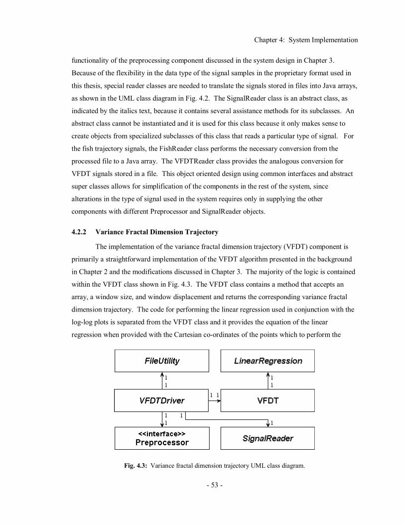
Chapter 4: System Implementation
- 53 -
functionality of the preprocessing component discussed in the system design in Chapter 3.
Because of the flexibility in the data type of the signal samples in the proprietary format used in
this thesis, special reader classes are needed to translate the signals stored in files into Java arrays,
as shown in the UML class diagram in Fig. 4.2. The SignalReader class is an abstract class, as
indicated by the italics text, because it contains several assistance methods for its subclasses. An
abstract class cannot be instantiated and it is used for this class because it only makes sense to
create objects from specialized subclasses of this class that reads a particular type of signal. For
the fish trajectory signals, the FishReader class performs the necessary conversion from the
processed file to a Java array. The VFDTReader class provides the analogous conversion for
VFDT signals stored in a file. This object oriented design using common interfaces and abstract
super classes allows for simplification of the components in the rest of the system, since
alterations in the type of signal used in the system requires only in supplying the other
components with different Preprocessor and SignalReader objects.
4.2.2 Variance Fractal Dimension Trajectory
The implementation of the variance fractal dimension trajectory (VFDT) component is
primarily a straightforward implementation of the VFDT algorithm presented in the background
in Chapter 2 and the modifications discussed in Chapter 3. The majority of the logic is contained
within the VFDT class shown in Fig. 4.3. The VFDT class contains a method that accepts an
array, a window size, and window displacement and returns the corresponding variance fractal
dimension trajectory. The code for performing the linear regression used in conjunction with the
log-log plots is separated from the VFDT class and it provides the equation of the linear
regression when provided with the Cartesian co-ordinates of the points which to perform the
Fig. 4.3: Variance fractal dimension trajectory UML class diagram.

Chapter 4: System Implementation
- 54 -
regression upon. The VFDTDriver abstract class connects the preprocessing and VFDT
components by utilizing a Preprocessor object to perform the preprocessing upon the raw data
files and to create files that can be read into an array by a SignalReader object. This array can
then be supplied to the VFDT class along with a desired window size and displacement in order
to obtain the VFDT. The FileUtility class is a multipurpose class used throughout this thesis to
assist in writing to and reading from files. The VFDTDriver uses this class to write the VFDT to
a file in the same proprietary format used by the preprocessing component, which can be later
read by a VFDTReader object.
4.2.3 Kohonen Self-Organizing Feature Map
The Kohonen self-organizing feature map (SOFM) implementation is constrained to
organizing its output neurons in a one dimensional configuration, as justified in the design of the
SOFM component. Logically, the network is composed of a number of neurons, thus the
functionality for the individual neurons are separated from the SOFM itself and is represented by
the KohonenNeuron class depicted in Fig. 4.4. The Kohonen1DSOFM class acts as the interface
for the SOFM, as it will construct the network out of a number of KohonenNeurons when
provided with the desired number of input and output neurons.
The Kohonen1DSOFM class also contains methods for training the network. The SOFM
training algorithm requires a number of different parameters, some of which are required
parameters, such as the number of epochs, the initial learning rate, and the initial radius of the
neighbourhood function. In order to limit the number of required parameters to a reasonable
level, some of the parameters are simply given predefined values, such as the minimum learning
Fig. 4.4: Kohonen self-organizing feature map UML class diagram.
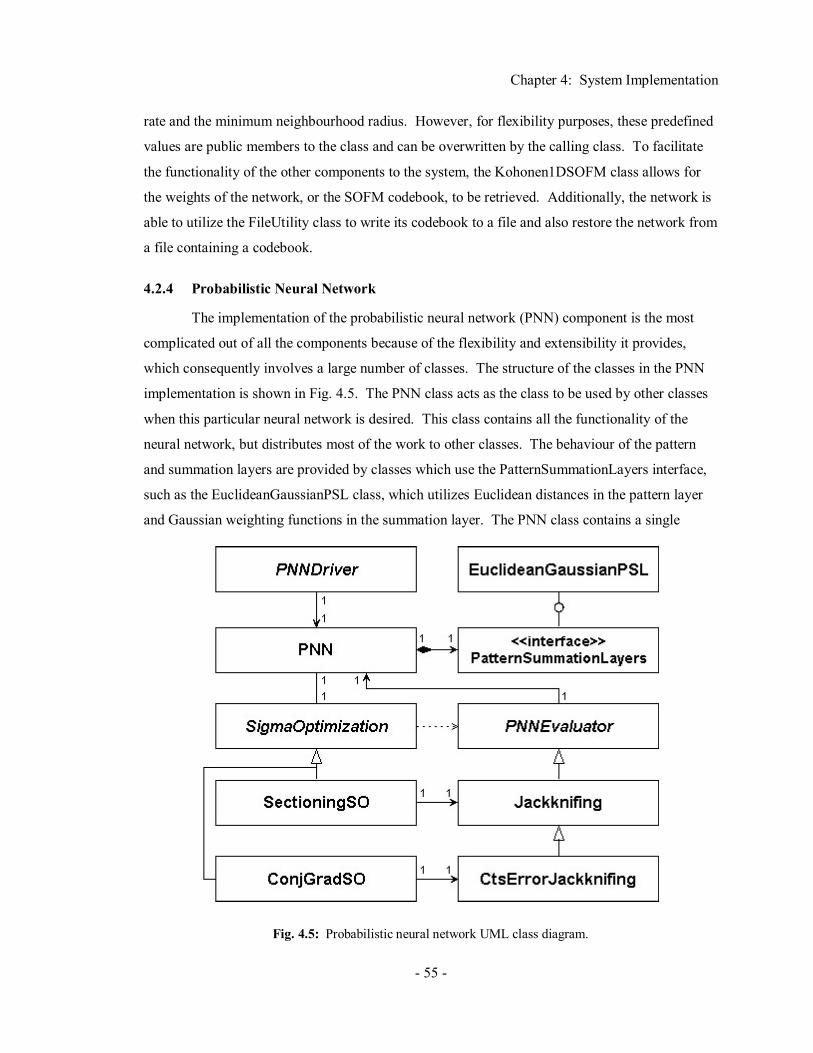
Chapter 4: System Implementation
- 55 -
rate and the minimum neighbourhood radius. However, for flexibility purposes, these predefined
values are public members to the class and can be overwritten by the calling class. To facilitate
the functionality of the other components to the system, the Kohonen1DSOFM class allows for
the weights of the network, or the SOFM codebook, to be retrieved. Additionally, the network is
able to utilize the FileUtility class to write its codebook to a file and also restore the network from
a file containing a codebook.
4.2.4 Probabilistic Neural Network
The implementation of the probabilistic neural network (PNN) component is the most
complicated out of all the components because of the flexibility and extensibility it provides,
which consequently involves a large number of classes. The structure of the classes in the PNN
implementation is shown in Fig. 4.5. The PNN class acts as the class to be used by other classes
when this particular neural network is desired. This class contains all the functionality of the
neural network, but distributes most of the work to other classes. The behaviour of the pattern
and summation layers are provided by classes which use the PatternSummationLayers interface,
such as the EuclideanGaussianPSL class, which utilizes Euclidean distances in the pattern layer
and Gaussian weighting functions in the summation layer. The PNN class contains a single
Fig. 4.5: Probabilistic neural network UML class diagram.
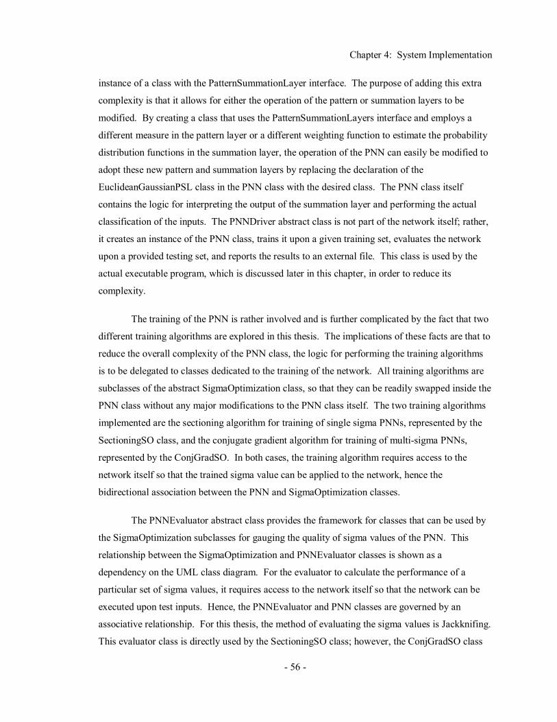
Chapter 4: System Implementation
- 56 -
instance of a class with the PatternSummationLayer interface. The purpose of adding this extra
complexity is that it allows for either the operation of the pattern or summation layers to be
modified. By creating a class that uses the PatternSummationLayers interface and employs a
different measure in the pattern layer or a different weighting function to estimate the probability
distribution functions in the summation layer, the operation of the PNN can easily be modified to
adopt these new pattern and summation layers by replacing the declaration of the
EuclideanGaussianPSL class in the PNN class with the desired class. The PNN class itself
contains the logic for interpreting the output of the summation layer and performing the actual
classification of the inputs. The PNNDriver abstract class is not part of the network itself; rather,
it creates an instance of the PNN class, trains it upon a given training set, evaluates the network
upon a provided testing set, and reports the results to an external file. This class is used by the
actual executable program, which is discussed later in this chapter, in order to reduce its
complexity.
The training of the PNN is rather involved and is further complicated by the fact that two
different training algorithms are explored in this thesis. The implications of these facts are that to
reduce the overall complexity of the PNN class, the logic for performing the training algorithms
is to be delegated to classes dedicated to the training of the network. All training algorithms are
subclasses of the abstract SigmaOptimization class, so that they can be readily swapped inside the
PNN class without any major modifications to the PNN class itself. The two training algorithms
implemented are the sectioning algorithm for training of single sigma PNNs, represented by the
SectioningSO class, and the conjugate gradient algorithm for training of multi-sigma PNNs,
represented by the ConjGradSO. In both cases, the training algorithm requires access to the
network itself so that the trained sigma value can be applied to the network, hence the
bidirectional association between the PNN and SigmaOptimization classes.
The PNNEvaluator abstract class provides the framework for classes that can be used by
the SigmaOptimization subclasses for gauging the quality of sigma values of the PNN. This
relationship between the SigmaOptimization and PNNEvaluator classes is shown as a
dependency on the UML class diagram. For the evaluator to calculate the performance of a
particular set of sigma values, it requires access to the network itself so that the network can be
executed upon test inputs. Hence, the PNNEvaluator and PNN classes are governed by an
associative relationship. For this thesis, the method of evaluating the sigma values is Jackknifing.
This evaluator class is directly used by the SectioningSO class; however, the ConjGradSO class

Chapter 4: System Implementation
- 57 -
utilizes a subclass of the Jackknifing class, the CtsErrorJackknifing class. This more specific
evaluator is required since the ConjGradSO class depends on the use of error gradients, or
derivatives, in its optimization of the sigma values, and the discretized Jackknifing evaluation is
insufficient.
The classes involved in the sectioning training algorithm are detailed in Fig. 4.6. As
previously discussed, the SectioningSO class utilizes the Jackknifing class to evaluate the
performance of a given sigma value. The sectioning algorithm itself utilizes two separate classes.
The purpose of this separation is two-fold. First, this separation is based on functionality, which
allows for substitutions of either of the components in cases where improvements to the basic
algorithm are desired. Second, the separation facilitates reuse of the classes. The GlobalLineMin
class performs the initial search through the problem space in an attempt to acquire a rough bound
of the optimal sigma value. This rough bound is then provided to a subclass of the
SectionLineMin class, for refinement. The SectionLineMin class performs the sectioning
algorithm whereby the interval thought to contain the optimal sigma value is progressively
reduced. The particular means in which the interval is reduced is provided by the
SectionLineMin class’s subclasses. The BisectionLineMin class dictates that the interval be
reduced by a factor of two in each iteration by simply calling the SectionLineMin’s refinement
method with a parameter of two. The choice of successively reducing the interval by two is
reasonable, but it should be noted that the interval can be reduced in any number of ways, some
Fig. 4.6: Sectioning sigma optimization UML class diagram.

Chapter 4: System Implementation
- 58 -
of which may take advantage of the nature of the problem space. One such alternative to
bisecting is utilizing the golden mean, 2 / (1 + √5), for reducing the intervals, as suggested in
[Mast95]. This modification was explored, but it did not produce any noticeable difference.
The conjugate gradient training component of the PNN is shown in more detail in Fig.
4.7. The ConjGradSO class utilizes the SectioningSO class in order to initiate the process by
optimizing for a single sigma PNN. The sigma values are then allowed to take on different values
and are optimized using a standard conjugate gradient algorithm, which is performed by the
ConjGradSO class. The GlobalLineMin class is reused here by the ConjGradSO class. The
BrentLineMin class, which performs Brent’s line minimization is also utilized by the
ConjGradSO class in executing the conjugate gradient algorithm The error derivates used in the
algorithm are provided by the CtsErrorJackknifing evaluator class, as previously mentioned.
4.2.5 Complex Domain Neural Network
The second classifier neural network used in this thesis is the complex domain neural
network. Complex numbers are not built into the Java language, so a ComplexNumber class is
implemented to represent complex numbers, using Cartesian co-ordinates, and perform basic
operations with complex numbers. This class contains a number of methods for complex number
arithmetic as well as operations mixing real and complex numbers in order to facilitate the
implementation of the complex domain neural network. These functions include addition,
subtraction, multiplication, division, and polar co-ordinate conversions.
The network itself is represented by the CNN class shown in Fig. 4.8, which is composed
of any number of neurons operating upon complex inputs. These neurons are implemented as the
ComplexNeuron class. Both classes utilize the ComplexNumber class extensively. The
Fig. 4.7: Conjugate gradient sigma optimization UML class diagram.
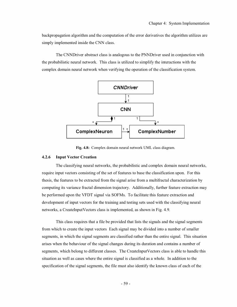
Chapter 4: System Implementation
- 59 -
backpropagation algorithm and the computation of the error derivatives the algorithm utilizes are
simply implemented inside the CNN class.
The CNNDriver abstract class is analogous to the PNNDriver used in conjunction with
the probabilistic neural network. This class is utilized to simplify the interactions with the
complex domain neural network when verifying the operation of the classification system.
4.2.6 Input Vector Creation
The classifying neural networks, the probabilistic and complex domain neural networks,
require input vectors consisting of the set of features to base the classification upon. For this
thesis, the features to be extracted from the signal arise from a multifractal characterization by
computing its variance fractal dimension trajectory. Additionally, further feature extraction may
be performed upon the VFDT signal via SOFMs. To facilitate this feature extraction and
development of input vectors for the training and testing sets used with the classifying neural
networks, a CreateInputVectors class is implemented, as shown in Fig. 4.9.
This class requires that a file be provided that lists the signals and the signal segments
from which to create the input vectors Each signal may be divided into a number of smaller
segments, in which the signal segments are classified rather than the entire signal. This situation
arises when the behaviour of the signal changes during its duration and contains a number of
segments, which belong to different classes. The CreateInputVectors class is able to handle this
situation as well as cases where the entire signal is classified as a whole. In addition to the
specification of the signal segments, the file must also identify the known class of each of the
Fig. 4.8: Complex domain neural network UML class diagram.
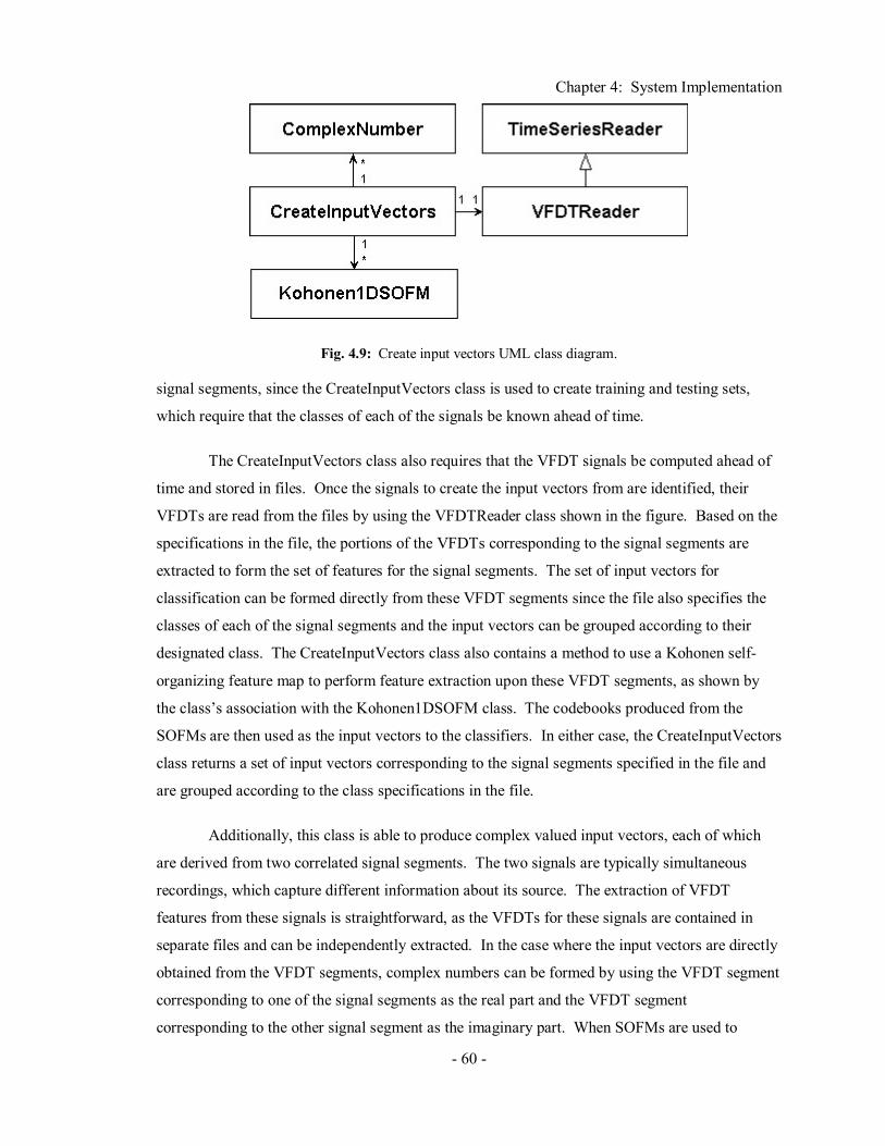
Chapter 4: System Implementation
- 60 -
signal segments, since the CreateInputVectors class is used to create training and testing sets,
which require that the classes of each of the signals be known ahead of time.
The CreateInputVectors class also requires that the VFDT signals be computed ahead of
time and stored in files. Once the signals to create the input vectors from are identified, their
VFDTs are read from the files by using the VFDTReader class shown in the figure. Based on the
specifications in the file, the portions of the VFDTs corresponding to the signal segments are
extracted to form the set of features for the signal segments. The set of input vectors for
classification can be formed directly from these VFDT segments since the file also specifies the
classes of each of the signal segments and the input vectors can be grouped according to their
designated class. The CreateInputVectors class also contains a method to use a Kohonen self-
organizing feature map to perform feature extraction upon these VFDT segments, as shown by
the class’s association with the Kohonen1DSOFM class. The codebooks produced from the
SOFMs are then used as the input vectors to the classifiers. In either case, the CreateInputVectors
class returns a set of input vectors corresponding to the signal segments specified in the file and
are grouped according to the class specifications in the file.
Additionally, this class is able to produce complex valued input vectors, each of which
are derived from two correlated signal segments. The two signals are typically simultaneous
recordings, which capture different information about its source. The extraction of VFDT
features from these signals is straightforward, as the VFDTs for these signals are contained in
separate files and can be independently extracted. In the case where the input vectors are directly
obtained from the VFDT segments, complex numbers can be formed by using the VFDT segment
corresponding to one of the signal segments as the real part and the VFDT segment
corresponding to the other signal segment as the imaginary part. When SOFMs are used to
Fig. 4.9: Create input vectors UML class diagram.

Chapter 4: System Implementation
- 61 -
extract features from the VFDT segments, the two VFDT segments corresponding to the two
signal segments are used as the training data for the SOFM. The input vectors to the SOFM
consist of appended portions of the VFDT segments, as explained in the design of the SOFM
component in Chapter 3. This ability of the CreateInputVectors class to produce complex valued
input vectors requires the use of the ComplexNumber class, as shown in Fig. 4.9.
4.2.7 Classifier Driver
The classifier driver programs are the only executable programs in the system and they
connect all the components together in order to form the various configurations of the
classification system. There are separate classifier driver programs for the configurations of the
system which use the probabilistic and complex domain neural networks, but they are identical
except that they use different classifier neural networks. Since the interface for the two networks
are very similar, their corresponding classifier driver programs differ only by a few lines.
The classifier driver for the PNN is shown in Fig. 4.10. The PNNClassifer driver is an
active class, indicated by the bold lines, meaning that it is executable. This class is responsible
for performing the preprocessing of the signals and computation of the VFDT signals. This work
is delegated to the VFDTDriver class. The training and testing sets are then formed through the
use of the CreateInputVectors class. Finally, the PNNDriver class is used to train the network
with the input vectors in the training set and also to classify the testing set input vectors. The
UML diagram for the classifier driver program that uses the complex domain neural network is
identical to that of Fig. 4.10, except that the classifier driver is named CNNClassifierDriver and it
uses the CNNDriver instead of the PNNDriver. The classifier driver programs require only that
the high level parameters such as the VFDT window size and displacement, the size of the SOFM
codewords, the number of codewords, and the specification of the training and testing sets be
provided. The values of these parameters are passed along to the corresponding components.
Fig. 4.10: Classifier driver UML class diagram.

Chapter 4: System Implementation
- 62 -
The final result of the execution of the driver program is a file summarizing the performance of
the classification system upon the testing set.
4.3 Summary
This section has discussed the implementation of the system and its components. While
the implementation of the system is finished, the overall development of the system is not
complete until it has been thoroughly tested and verified.

Chapter 5: System Verification and Testing
- 63 -
CHAPTER 5
SYSTEM VERIFICATION AND TESTING
The necessity of testing and verifying any design, whether it be software or hardware, is
of paramount importance. Testing and verification must be performed upon a system in order to
ascertain whether the results it produces are valid. The testing and verification of the software
used in this thesis is subdivided into two distinct sections. First, each of the individual, distinct
components of the system underwent separate tests to ensure their accuracy. Afterwards, testing
and verification of the system as an integrated whole was performed to ensure that the resulting
system performed as expected.
5.1 Component Verification and Testing
5.1.1 Preprocessing
The primary verification of the functionality of the preprocessing component is the
confirmation that the data conversion performs without introducing any error into the signals. In
order to perform this verification, a signal was read from its raw data file and then from the
processed file. The values read were then compared visually by plotting the two signals side by
side and numerically by comparing the signals sample by sample. Both plotted signals appeared
as expected, demonstrating that the signals were read correctly and the numerical verification
demonstrated that the conversion was error free.
5.1.2 Variance Fractal Dimension Trajectory
The calculations involved with the VFDT algorithm for even small signals are a
computationally heavy process. Thus, it was determined that verifying the system by hand would
be far too lengthy a process. As a result, other methods of verification, both subjective and
objective, were selected to verify the correctness of the VFDT component.
While the VFDT algorithm itself is too involved to verify by hand, the linear regression
used by the algorithm is simple and ubiquitous enough to independently confirm its correct
operation. The linear regression was provided with some points in a Cartesian plane and the
equation of the resulting regression was obtained. These values were then confirmed by
Chapter 5: System Verification and Testing
- 64 -
performing the identical operations by hand and independently verifying the values by using a
mathematical program to perform the regression.
The verification of the operation of the VFDT component was performed mostly by
computing the VFDT of various simulated power line transients and comparing the results to
those found in [Chen01]. The plots resulting from the VFDT component developed for this thesis
and those of the published plots correlated, thus providing a high level verification of the
implementation of the algorithm.
Another subjective measure used to verify the VFDT component was that by visual
inspection of the plots of the VFDT signals, it was observed that the signals were, for the most
part, bound between the theoretical limits of one and two. Furthermore, the signal was reasonable
in that it seemed to emphasize the changes in the original signal. Additionally, changes to the
window size and displacement yielded expected results whereby decreasing the displacement
increased the resolution of the VFDT signal and differing window sizes controlled the amount of
smoothing that occurred.
Lastly, it should be noted that the artifacts caused by straight lines and certain
periodicities in the sample domain signal were discovered during the testing and verification of
this component and modifications were made to the component during the iterative design
process to reduce the effect of these artifacts, as discussed in Chapter 3. With the modification to
the VFDT algorithm, the verification of the reduction of the artifacts was observed. By
comparing the individual samples of the VFDT signals before and after the modification to the
algorithm, it was observed that the difference was minimal, confirming the infrequency in
occurrence of these artifacts.
5.1.3 Kohonen Self-Organizing Feature Map
The Kohonen self-organizing feature map (SOFM) component was tested by tracing
through the code and performing some hand calculations and verified using toy problems. Hand
computations were performed first in order to ensure the operation of the neurons and the synapse
weight training. After completing manual calculations, the correctness of the SOFM component
was verified by training the SOFM with several groups of sinusoidal signals of varying
amplitudes, frequencies, and phase, along with noise. The resulting codebook was plotted and it
was visually seen that distinct clusters had formed, each of which were characteristic of the
sinusoidal signal classes. Further tests were performed to verify the SOFM’s ability to perform
Chapter 5: System Verification and Testing
- 65 -
feature extraction of signals. In once instance, the SOFM was instructed to form a representative
codebook of a complicated signal. This trained codebook was used to perform learned vector
quantization of the original signal. Each interval of the original signal was replaced with the best
matched codeword in the codebook, producing a signal formed entirely from the codewords in
the codebook. Visually, the resulting signal was very similar to the original signal, even though
the number of codewords was mere a fraction of the total number of interval segments in the
signal itself. By computing the mean square error between the two signals, it was noted that
numerically, the signals were fairly different, but considering the amount of compression
achieved, the result was acceptable. This learned vector quantization verified the feature
extraction capabilities of the SOFM.
5.1.4 Probabilistic Neural Network
The probabilistic neural network component was tested using a small number of hand
calculations and verified quite extensively by the use of toy problems. The hand calculations
were primarily used to confirm that the mathematical calculations in layers of the network were
being correctly calculated. Specifically, the program was traced so as to ensure that the neurons
in the pattern layer were calculating the Euclidean distance between the input to the neural
network and the training input correctly. The output of the weighting function of each of the
pattern layer neurons was also verified by hand. Additionally, the calculations performed by the
neurons in the summation layer were performed by hand to ensure that the scaled estimations of
the PDFs generated by the neurons were correct.
The verification of the PNN was performed by evaluating its performance on toy
problems. One of the main toy problems used to test the operation of the PNN was to simply
create k different classes of points in n-dimensional space. The PNN was trained using various
example training inputs from each of the k classes. To verify that the PNN was capable of
learning and generalizing, the PNN was then tested with samples from the classes that were not
present in the training set. The level of difficulty of these point-clustering toy problems ranged
from very easy, when each class consisted of a single cluster of points, to more challenging,
where some of the classes were multimodal and the cluster borders overlapped. The PNN
performed very well on all of the toy problems, including those which involving multimodal
classes, typically obtaining correct classification rates well above 90%.
Chapter 5: System Verification and Testing
- 66 -
The multi-sigma PNN was also tested using toy problems with classes of points in n-
dimensional space. With the multi-sigma PNN, the classes of points were designed such that
some of the class clusters spanned a wide area, while others were very tight and well defined.
This type of toy problem demonstrated that the multi-sigma training algorithm was capable of
selecting different sigma values, depending on the relative size of the class clusters. Accordingly,
the sigma values selected for classes whose points spanned a wide area received larger sigma
values, while the classes whose points were confined to a very tight area were assigned smaller
sigma values.
5.1.4.1 Line Minimization
The verification of the line minimization algorithm used in the training of the PNN
component was straightforward, as direct inspection could be performed. Specifically, the line
minimization component was tested using several higher order polynomials containing a variety
of local minima and maxima. The line minimization module was then configured to attempt to
discover an acceptable minimum over a particular portion of these functions. Effort was made to
ensure that the section used for the minimum search contained several different minima and
maxima, thereby confirming the fact that the optimization problem was not trivial.
Upon running the line minimization program on several higher order polynomials, the
component usually yielded the absolute minimum within the specified interval. There were
however, instances in which the program did not find the global minimum, and instead,
discovered a local minimum. The reason the algorithm did not always uncover the global
minimum was not a flaw in the implementation of the component, but rather a problem in the
algorithm itself. During the first stage of the line minimization process, the algorithm selects
several trial points at which it evaluates the function. The trial point that yields the smallest result
is assumed to be very close to the global minimum of the function, so the area immediately
surrounding that point is searched to find the minimum. However, the assumption that the global
minimum is close to the smallest result found in the first stage of the algorithm may not always be
valid.
In the simple example shown in Fig. 5.1, the line minimization algorithm selects three
trial points, which is an unreasonably small number, but has been chosen for explanation
purposes only. As can be seen in the figure, of the selected three points indicated by the arrows,
the point on the extreme left yields the smallest function value of the three. Hence, the second

Chapter 5: System Verification and Testing
- 67 -
step of the line minimization algorithm will look for the minimum in the area immediately
surrounding this trial point. Of course, in doing so, the algorithm will find the local minimum
between the X-axis values of 1 and 1.5. As can be seen in the figure, there is a superior minimum
located between the X-axis values of 4.5 and 5 that was not identified by the algorithm.
This specific difficulty with the algorithm was recognized before the testing process was
undertaken, but was not considered to be of large concern. If the number of trial points in this
example were increased to a more reasonable number, such as 15, then the true global minimum
would have been identified. This line minimization is being used in this thesis to optimize the
smoothing parameter(s) of the PNN, which, as was noted earlier in this paper, generally tends to
have a region of values which are acceptable. Hence, more importance was placed on finding a
reasonable local minimum in a short period of time, as opposed to finding the absolute global
minimum through a lengthier search.
Despite the fact that the algorithm was designed with the knowledge that it might not
always uncover the absolute minimum within a given interval, the algorithm was shown to
operate correctly through the testing and verification stage.
1 1.5 2 2.5 3 3.5 4 4.5 5-8
-7
-6
-5
-4
-3
-2
-1
0
1
2
x
y
Fig. 5.1: Erroneous selection of bounded minimum.
Chapter 5: System Verification and Testing
- 68 -
5.1.5 Complex Domain Neural Network
As was the case with most of the components implemented in this thesis, the testing of
the complex domain neural network was difficult to perform thoroughly by virtue of the fact that
its computations were so numerous. As a result, it would have been time consuming to fully
verify the algorithm’s calculations by hand. Nonetheless, the correctness of the neural network
was verified through a combination of hand calculations and toy problems.
Initially, the complex domain neural network using the backpropagation training
algorithm was verified with hand calculations. The computations were performed by hand on a
simple toy problem where the neural network implemented a very simple parity checker
involving only two inputs, one hidden neuron, and one output neuron. The calculations focused
on ensuring that the hidden layer neurons computed the correct net sums, and that the results of
the activation functions were accurate. Additionally, some of the partial derivatives used in the
actual backpropagation algorithm were performed by hand to ensure that the algorithm was
implemented correctly. Furthermore, updating of the synapse weights was verified by hand. The
hand calculations were limited only to the first few iterations, as attempting to perform full
verification through the thousands of iterations was overtly cumbersome. These limited
calculations that were performed by hand did help to ensure that all the mathematical formulas
had been programmed correctly.
After the hand verification of the complex neural network was completed, the next step
was to confirm that it was capable of learning, generalizing, and operating correctly as a whole.
To that end, a more complicated parity testing toy problem was utilized as well as a classification
problem in an n-dimensional space similar to that used with the PNN. The complex neural
network was able to correctly identify the parity of the various inputs in the testing set and
perform the classification of points in an n-dimensional space. In both cases, the neural network
correctly performed the operation on the testing set well above 90%, indicating that the
component was operating overall as anticipated.
5.2 Overall System Verification and Testing
In addition to performing testing and verification of all the individual components created
for this thesis, it was still necessary to verify that when all those components were interconnected,
the overall system would operate correctly. The overall system operation was verified through

Chapter 5: System Verification and Testing
- 69 -
the use of simulated signals. By creating signals with known class memberships, such as power
line transients used in [Chen01], the classification system using the PNN component was verified
by performing classification of these signals using both the VFDT and SOFM components to
perform feature extraction. Initially, the correct classification rates obtained by the system were
not as high as expected, achieving rates only in the low 70% range. However, further
examination showed that the less than spectacular results were caused because the system was
consistently unable to classify signals from particular classes. In these classes, the simulated
power line transients only exhibited simple transitions and were not fractal in nature, hence,
according to their VFDT signals, they were all the same. By grouping these simple transients into
a single class, the resulting classification results showed much improvement, correctly classifying
the signals above 90% of the time.
In order to further verify the various configurations of the system, additional tests using a
small subset of the fish trajectory signals and assumed classes based upon a priori knowledge of
the experiment were performed. The different system configurations, including the complex
domain neural network and the probabilistic neural network with complex inputs based systems,
did, for the most part, successfully perform the requested classification. The results however, will
not be quoted here as the classes which the classification was based upon were very limited and
not known to be true.
The only problem that was encountered during system testing and verification was that
the multi-sigma training algorithm was not able to operate successfully with the fish trajectory
signals. During training, the error derivatives unexpectedly become zero, causing the algorithm
to fail. It is suspected that the cause of the problem was the size of the classification problem and
the limited precision of the floating point values used in the PNN component. Thus, due to these
complications which were not resolvable within the time limits of this thesis, the PNN multi-
sigma training will not be further examined.
5.3 Summary
The verification and testing of the classification system and its components were
discussed in this section of the thesis. Aside from the multi-sigma PNN, no difficulties were
encountered. The remaining task is to verify that the classification system indeed works well
upon stochastic, self-similar, non-stationary signals arising from non-linear systems.

Chapter 6: Experimental Results and Discussion
- 70 -
CHAPTER 6
EXPERIMENTAL RESULTS AND DISCUSSION
In this section, the experiments used to formally verify and compare the various
configurations of the system will be presented and explained. The classification system begins
with a preprocessing stage to convert the signals into the format used in this thesis. Following the
preprocessing stage, a multifractal analysis is performed whereby the signal is transformed into
the fractal dimension domain to produce a variance fractal dimension trajectory (VFDT). In one
configuration of the system these fractal dimensions are directly used as features for the
classification process. In the second, Kohonen self organizing feature maps (SOFMs) are used to
extract the features from the VFDT signal in an attempt to eliminate redundancy while
simultaneously reducing the size of the classification problem. To perform the classification
based on the extracted features, this thesis explores two different types of neural networks:
probabilistic neural networks (PNN) and complex domain neural networks (CNN). The signals
used to verify the various configurations of the system consist of two recordings. The extent to
which classification can be performed with a single recording is explored through the use of the
PNN. Further experiments upon the system are performed by classifying the signals while taking
into consideration features from both recordings via the PNN and CNN in separate experiments.
6.1 Experiment Set-Up
The particular verification signals used in this thesis are fish trajectory recordings
produced from a tracking system that monitors the position of a fish in a fish tank along the X, Y
and Z axes when presented with various stimuli, as explained in Appendix A. Seventeen of these
recordings have been obtained and are used for the formal experiments. Of the 17 recordings,
nine involve one particular fish while the remaining eight concern a different fish. Ordinarily,
class specifications and examples from each of the classes would be available to construct the
training and testing sets which are used to train the classification system and evaluate its
performance. These specifications were not available for the fish trajectory signals. Since
training and testing sets are a necessity, an objective method in deriving these sets was sought. It
was decided that clustering upon the time domain signals using an SOFM would be an
appropriate vehicle to arrive at the desired class specifications. A full discussion of the derivation
of the training and testing sets is presented in Appendix B.

Chapter 6: Experimental Results and Discussion
- 71 -
This thesis is not concerned about the classification of the fish signals per se, but rather in
using them in order to verify the system. Thus, the two most important axes, X and Z, are used
since the CNNs only operate on two simultaneous recordings.
Through the clustering performed upon the signals in Appendix B, it was shown that four
different classes were present in each signal when they were divided into segments of 4096
samples, which corresponds to just under seven minutes. All the segments from nine of the files
were dedicated to the training set, while the segments from the other eight were delegated to act
as the testing set. Both the training and testing sets have approximately equal number of
recordings from both of the fish. It is important to note that the training and testing sets are
mutually exclusive so as to provide an unbiased performance assessment of the various
configurations of the classification system.
With the training and testing sets established, the classification of the signals can actually
be performed. Preprocessing is the first task that must be executed so as to put the signals into
the propriety format used by the rest of the components in their analysis. The recordings along
Fig. 6.1: Time domain plots of a fish trajectory signal.

Chapter 6: Experimental Results and Discussion
- 72 -
the X and Z axes for a sample signal following the preprocessing stage are plotted in Fig. 6.1.
The time required to perform this preprocessing for each signal is approximately four and a half
minutes on a 1 GHz AMD Athlon computer.
The next stage of the classification system involves computing the VFDT of the signals
for the purpose of feature extraction. There are two parameters involved in calculating the
VFDT: window size and the displacement of the windows. Normally the window size would be
decided upon based on the largest stationarity of the signal; however not enough is known about
the fish trajectory signals, so the window size had to be determined experimentally. It was
discovered that a window size of 2048 and window displacement of 256 provided the best results
in that the combination yielded a good balance between an adequate resolution and substantial
reduction in the problem size. Because of this displacement, 256 samples in the sample domain
correspond to one sample in the VFDT, thus the 4096 samples in each segment are represented by
only 16 fractal dimensions. The plots of the VFDT signals corresponding to the signals of Fig.
6.1 are shown in Fig. 6.2. The processing time required to computer these plots for each axis is
Fig. 6.2: VFDTs of a fish trajectory signal.

Chapter 6: Experimental Results and Discussion
- 73 -
only a third of a second. The first thing to note about the VFDT plots is that the fractal dimension
of the signals change, indicating that it is a multifractal. It can further be noted that the samples
of the VFDT are normalized between dimensions of one and two, which is essential for the
classification process. Additionally, the VFDT plots visually seem to correspond to the time
domain plots in that they tend to emphasize some of the characteristics in the original signal; the
most exemplary characteristic being the initial dramatic changes in the VFDT signals which
correspond to the irregular motion of the fish as seen in the time domain plot. The VFDT plots
shown are characteristic of all the fish trajectory VFDTs.
In calculating the VDFT, log-log plots were produced and linear regressions upon the
points in these plots were computed as per the VFDT algorithm as presented in Chapter 2. As a
means of evaluating the signal’s accordance to the power law behaviour, mean square errors
(MSEs) between the linear regression and the sample points in these log-log plots are tabulated in
a histogram format, as shown in Fig. 6.3, which correspond to the VFDT signals in Fig. 6.2. The
vast majority of the MSEs are low, which indicates that the power law behaviour is exhibited
Fig. 6.3: MSE histogram of the VFDT of the fish trajectory signal.

Chapter 6: Experimental Results and Discussion
- 74 -
throughout most of the signal. There are some outliers where the MSE is more substantial but
their occurrence is very seldom. This adherence to the power law behaviour indicates that the
particular window size is valid for the signal and furthermore, that indeed that the signal is fractal
in nature.
Segmentation of the VFDT signals is performed at this stage in such a manner to
correspond to the time domain segments of length 4096 as defined for the training and testing
sets. These VFDT segments are the features for classification.
In the configurations of the system using the SOFM, feature extraction is performed upon
these VFDT segments. The SOFMs can be used to extract features from VFDT segments which
consist of a single recording or multiple recordings. In order to facilitate the extraction of
features from segements involving multiple recordings, the recordings are merely appended to
each other prior to being presented to the SOFM as was shown in Eq. (3.1).
For the formal experiments used to verify the different configurations of the classification
system, the SOFM was configured to use three codewords, each of which had a length of four.
This combination means that 12 features are extracted from each VFDT segment. The
configuration of three codewords with a length of four apiece was selected as experimentally it
yielded very good results. Scenarios where fewer codewords were used usually produced decent
results and decreased the problem size even further. However, the overall classification accuracy
decreases with fewer codewords. Since none of the systems take more than a few seconds to
execute, it was decided to make use of more codewords instead of reducing the problem size as
much as possible.
Figure 6.4 shows a sample segment of a VFDT and its corresponding SOFM codebook.
The codebook contains the codewords most representative of the signal and it should also be
noted that the classification problem size is reduced during the transition from the VFDT segment
to the SOFM codebook in that the number of features used to represent the signal segment is
reduced. The generation of the all the codebooks for the entire training and testing sets require no
more than a third of a second, whether it be for a single recording signal or a multiple recording
signal. In the configurations of the system involving the SOFM component, it is these codebooks
and their codewords that are provided as inputs into the neural networks rather than the VFDT as
is done when the SOFM module is not used.

Chapter 6: Experimental Results and Discussion
- 75 -
6.2 Results
6.2.1 Experiment 1: X-Axis with PNN
For the first experiment, the VFDT segments corresponding the X-axis were directly used
to form training and testing sets for use with the PNN. It took approximately four seconds to
train the PNN and less than a fifth of a second to classify the entire testing set consisting of 544
input vectors. The results of the testing set classification are summarized in the confusion matrix
shown in Table 6.1. The rows of the confusion matrix indicate the expected class of a particular
signal segment, as defined in the testing set, whereas the columns indicate the experimental
classification result produced by the PNN. The count in any given cell is the corresponding
number of signal segments from the testing set which the PNN considered to belong to that class.
As a result, the entries along the diagonal indicate the number of correct classifications for a
given class whereas cells off the diagonal indicate incorrect classifications where the PNN
identified the signal segment as belonging to a class different than was expected. The column on
Fig. 6.4: VFDT segment and its codebook.
Table 6.1: X-axis PNN confusion matrix.
Experimental
1 2 3 4
Correct Classification
Rate 1 24 0 0 0 100.00%
2 3 135 4 4 92.47%
3 0 12 111 65 59.04%
Expe
cted
4 0 23 70 93 50.00%
Average Correct Classification Rate: 66.73%
95% Confidence Interval: [62.77%, 70.69%]

Chapter 6: Experimental Results and Discussion
- 76 -
the extreme right indicates the percent correct classification for each of the individual classes.
With respect to the first experiment, the table show that all 24 inputs from class 1 were classified
correctly, yielding a classification accuracy of 100%. For the second class, three inputs were
erroneously considered to belong to class one, four inputs to class three, and four inputs to class
four. However, the classification system correctly identified 135 inputs as belonging to class two,
which meant that class two had a correct classification rate of 92.47%. This same analysis
procedure can be performed for the remaining rows of the confusion matrix.
The average classification rate, shown below the confusion matrix, is the overall
performance indicator of the network and is the ratio of the number of correct classifications to
the total number of signal segments presented to the network. For example, in this experiment
the average classification rate is calculated by (24 + 135 + 111 + 93) / 544 * 100%. For this
experiment, the average classification rate is approximately 67%. Despite the overall poor
performance, the system did function quite well with respect to the first two classes. However,
the network was simply not able to differentiate between the last two classes with much success.
Although 67% is not a substantially high correct classification rate, if the system were to perform
classification by randomly guessing to which class an input signal belongs, then the expected rate
of classification would only be 25%. In that regard, 67% shows that there is confidence that the
system is able to analyze the signal and is not just performing arbitrary assignments. However, a
67% correct classification rate is still far from the desired rate of 90%.
Since randomness is involved in the particular selection of the testing sets, confidence
intervals are computed. These particular intervals show the range of values within which the true
classification rate falls, with a confidence of 95%. The computation of the confidence intervals
for the average classification rate comes from the binomial distribution, in that each input vector
to the neural network is either correctly or incorrectly classified. The estimation of the standard
deviation about the true mean is given by (1 ) /s r r n= − , where r is the average classification
rate and n is the total number of input vectors in the testing set. The 95% confidence intervals are
defined by [r – 1.96s, r + 1.96s]. For this experiment, it can be stated that the true mean
classification rate falls between 62.77% and 70.69% with a 95% confidence. This experiment did
not produce a correct classification rate as high as desired, even when the confidence intervals are
taken into consideration; however, this experiment only made use of the information in the X-axis
recordings. The additional inclusion of the information contained in the Z-axis during the
classification process should increase the classification rate.

Chapter 6: Experimental Results and Discussion
- 77 -
6.2.2 Experiment 2: X-Axis with SOFM and PNN
The second experiment performed was similar to the first experiment in that only the X-
axis information from the fish trajectory signals was used to perform classification. What
differentiates these two experiments is the fact that the second experiment made use of the SOFM
component to perform feature extraction upon the VFDT signal whereas the first experiment did
not.
The inclusion of the SOFM feature extraction process did not improve the overall
classification rate of the system as indicated by the average classification rate seen in Table 6.2.
Making use of the SOFMs did, however, reduce the number of inputs into the PNN from 16 in
experiment one to 12 in experiment two, which caused a reduction in the training and execution
times of the system. Hence the SOFM stage did not improve the overall classification accuracy
of the system, but it did reduce the classification problem size, which expedites the classification
process. Specifically, the training time was reduced to a little less than three seconds while the
execution time was closer to a tenth of a second.
One important aspect to note about the confusion matrix for experiment two is that the
classification system was able to distinguish between the first three classes with a good deal of
success, but was unable to perform effective classification upon the fourth class.
Overall, no conclusions can be drawn as to whether the system configuration presented in
this second experiment provided superior classification accuracies than the first because the
confidence intervals overlap. As with the first experiment, the performance of the classification
system in this particular configuration is disappointing.
Table 6.2: X-axis SOFM PNN confusion matrix.
Experimental
1 2 3 4
Correct Classification
Rate 1 24 0 0 0 100.00%
2 4 131 8 3 89.73%
3 0 16 131 41 69.68%
Expe
cted
4 0 29 84 73 39.25%
Average Correct Classification Rate: 65.99%
95% Confidence Interval: [62.01%, 69.97%]
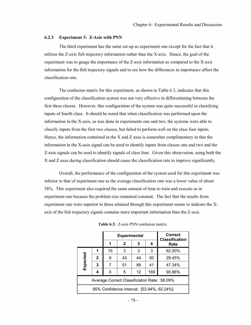
Chapter 6: Experimental Results and Discussion
- 78 -
6.2.3 Experiment 3: Z-Axis with PNN
The third experiment has the same set-up as experiment one except for the fact that it
utilizes the Z-axis fish trajectory information rather than the X-axis. Hence, the goal of the
experiment was to gauge the importance of the Z-axis information as compared to the X-axis
information for the fish trajectory signals and to see how the differences in importance affect the
classification rate.
The confusion matrix for this experiment, as shown in Table 6.3, indicates that this
configuration of the classification system was not very effective in differentiating between the
first three classes. However, this configuration of the system was quite successful in classifying
inputs of fourth class. It should be noted that when classification was performed upon the
information in the X-axis, as was done in experiments one and two, the systems were able to
classify inputs from the first two classes, but failed to perform well on the class four inputs.
Hence, the information contained in the X and Z axes is somewhat complimentary in that the
information in the X-axis signal can be used to identify inputs from classes one and two and the
Z-axis signals can be used to identify signals of class four. Given this observation, using both the
X and Z axes during classification should cause the classification rate to improve significantly.
Overall, the performance of the configuration of the system used for this experiment was
inferior to that of experiment one as the average classification rate was a lower value of about
58%. This experiment also required the same amount of time to train and execute as in
experiment one because the problem size remained constant. The fact that the results from
experiment one were superior to those attained through this experiment seems to indicate the X-
axis of the fish trajectory signals contains more important information than the Z-axis.
Table 6.3: Z-axis PNN confusion matrix.
Experimental
1 2 3 4
Correct Classification
Rate 1 15 3 3 3 62.50%
2 9 43 44 50 29.45%
3 7 51 89 41 47.34%
Expe
cted
4 0 5 12 169 90.86%
Average Correct Classification Rate: 58.09%
95% Confidence Interval: [53.94%, 62.24%]
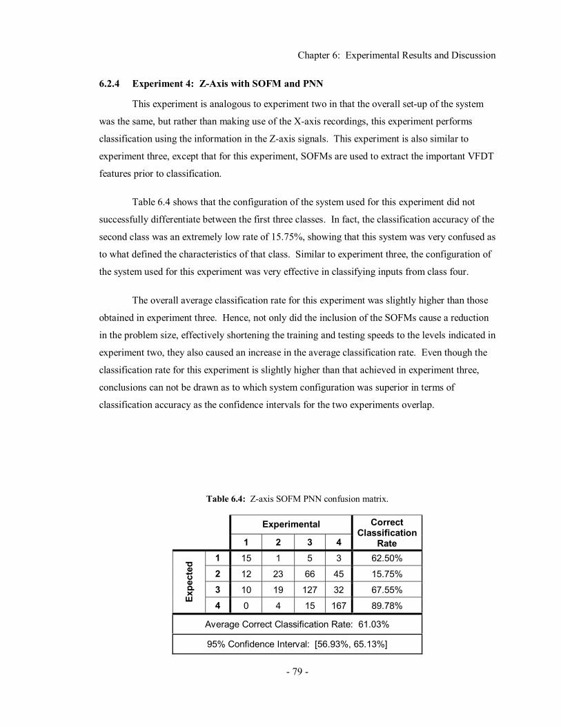
Chapter 6: Experimental Results and Discussion
- 79 -
6.2.4 Experiment 4: Z-Axis with SOFM and PNN
This experiment is analogous to experiment two in that the overall set-up of the system
was the same, but rather than making use of the X-axis recordings, this experiment performs
classification using the information in the Z-axis signals. This experiment is also similar to
experiment three, except that for this experiment, SOFMs are used to extract the important VFDT
features prior to classification.
Table 6.4 shows that the configuration of the system used for this experiment did not
successfully differentiate between the first three classes. In fact, the classification accuracy of the
second class was an extremely low rate of 15.75%, showing that this system was very confused as
to what defined the characteristics of that class. Similar to experiment three, the configuration of
the system used for this experiment was very effective in classifying inputs from class four.
The overall average classification rate for this experiment was slightly higher than those
obtained in experiment three. Hence, not only did the inclusion of the SOFMs cause a reduction
in the problem size, effectively shortening the training and testing speeds to the levels indicated in
experiment two, they also caused an increase in the average classification rate. Even though the
classification rate for this experiment is slightly higher than that achieved in experiment three,
conclusions can not be drawn as to which system configuration was superior in terms of
classification accuracy as the confidence intervals for the two experiments overlap.
Table 6.4: Z-axis SOFM PNN confusion matrix.
Experimental
1 2 3 4
Correct Classification
Rate 1 15 1 5 3 62.50%
2 12 23 66 45 15.75%
3 10 19 127 32 67.55%
Expe
cted
4 0 4 15 167 89.78%
Average Correct Classification Rate: 61.03%
95% Confidence Interval: [56.93%, 65.13%]

Chapter 6: Experimental Results and Discussion
- 80 -
6.2.5 Experiment 5: X and Z-Axis with PNN
Building off the idea that greater classification rates may be possible if both the X and Z
axes are utilized, this experiment focuses on the case where both axes are taken into consideration
when performing classification with the PNN.
The system used for this experiment performed at a consistently high rate for all of the
different classes. The individual classification rates for each class were all above 90% except for
class three. When the X and Z axes were used independently for classification, as was the case
for experiments one through four, class three consistently had a fairly low classification rate.
Thus, it is not all that surprising that the when the classification system uses information from
both X and Z-axis that it still has difficulties with class three.
Overall this experiment produced the highest average classification rate of any of the
experiments and the results are summarized in Table 6.5. The slight drawback of this
configuration of the system when compared to the systems outlined in experiments one though
four is that this system takes approximately twice as long to run since the classification problem
size is twice as large. However, in this case that meant that the classification system took
approximately seven seconds to train and a quarter of a second to execute, which is still very fast
and meets the time-based design constraints. This is also the one system that meets the design
constraint of at least a 90% average correct classification rate.
Table 6.5: X and Z-axis PNN confusion matrix.
Experimental
1 2 3 4
Correct Classification
Rate 1 24 0 0 0 100.00%
2 3 139 2 2 95.21%
3 0 12 157 19 83.51%
Expe
cted
4 0 9 1 176 94.62%
Average Correct Classification Rate: 91.18%
95% Confidence Interval: [88.80%, 93.56%]

Chapter 6: Experimental Results and Discussion
- 81 -
6.2.6 Experiment 6: X and Z-Axis with SOFM and PNN
This experiment is analogous to experiments two and four where the SOFMs are used in
an attempt to improve classification. However, for this experiment, rather than simply using the
X or Z-axis independently, this experiment considers both axes when developing the codebooks
used for classification.
As with experiment seven, the system configuration used in this experiment produced
very good results. Test inputs were classified quite successfully for each of the classes and the
average classification rate was a respectable 87.68%, as shown in Table 6.6. From this data it
cannot be determined whether the system used for this experiment was outperformed by the
configuration from experiment five because the average classification rate confidence intervals
overlap. However the execution time of the system used for this experiment is less than that of
the system in experiment five because it only took a little more than three seconds to train and a
sixth of a second to execute. Hence, the system used for this experiment yielded a classification
rate almost as high, if not as high as that of experiment five’s system, while requiring less training
and execution time.
6.2.7 Experiment 7: X and Z-Axis with CNN
Although experiments six and seven showed that the PNN is capable of classifying the
fish trajectory signals at very high classification rates by appending information from the X and Z
axes together, further experiments were performed to see how well a complex domain neural
network would perform. The PNN was not designed to be used in conjunction with complex
valued signals, but the complex domain neural networks were explicitly created for that purpose.
Table 6.6: X and Z-axis SOFM PNN confusion matrix.
Experimental
1 2 3 4
Correct Classification
Rate 1 23 1 0 0 95.83%
2 2 133 5 6 91.10%
3 0 14 161 13 85.64%
Expe
cted
4 0 19 7 160 86.02%
Average Correct Classification Rate: 87.68%
95% Confidence Interval: [84.92%, 90.44%]
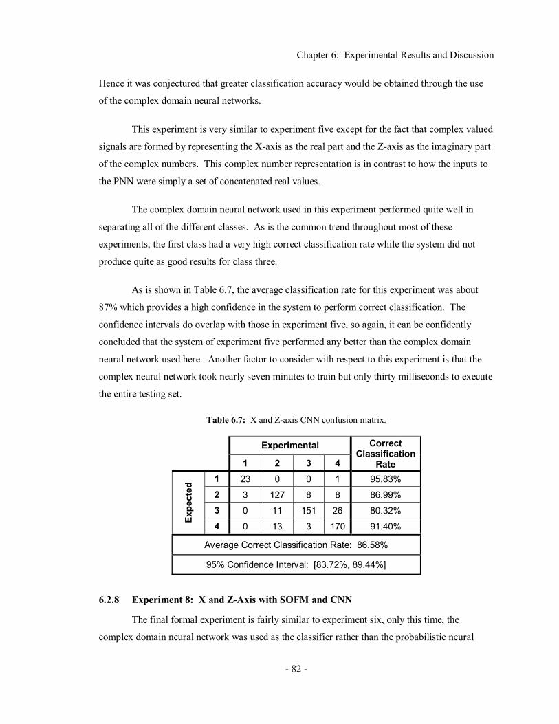
Chapter 6: Experimental Results and Discussion
- 82 -
Hence it was conjectured that greater classification accuracy would be obtained through the use
of the complex domain neural networks.
This experiment is very similar to experiment five except for the fact that complex valued
signals are formed by representing the X-axis as the real part and the Z-axis as the imaginary part
of the complex numbers. This complex number representation is in contrast to how the inputs to
the PNN were simply a set of concatenated real values.
The complex domain neural network used in this experiment performed quite well in
separating all of the different classes. As is the common trend throughout most of these
experiments, the first class had a very high correct classification rate while the system did not
produce quite as good results for class three.
As is shown in Table 6.7, the average classification rate for this experiment was about
87% which provides a high confidence in the system to perform correct classification. The
confidence intervals do overlap with those in experiment five, so again, it can be confidently
concluded that the system of experiment five performed any better than the complex domain
neural network used here. Another factor to consider with respect to this experiment is that the
complex neural network took nearly seven minutes to train but only thirty milliseconds to execute
the entire testing set.
6.2.8 Experiment 8: X and Z-Axis with SOFM and CNN
The final formal experiment is fairly similar to experiment six, only this time, the
complex domain neural network was used as the classifier rather than the probabilistic neural
Table 6.7: X and Z-axis CNN confusion matrix.
Experimental
1 2 3 4
Correct Classification
Rate 1 23 0 0 1 95.83%
2 3 127 8 8 86.99%
3 0 11 151 26 80.32%
Expe
cted
4 0 13 3 170 91.40%
Average Correct Classification Rate: 86.58%
95% Confidence Interval: [83.72%, 89.44%]
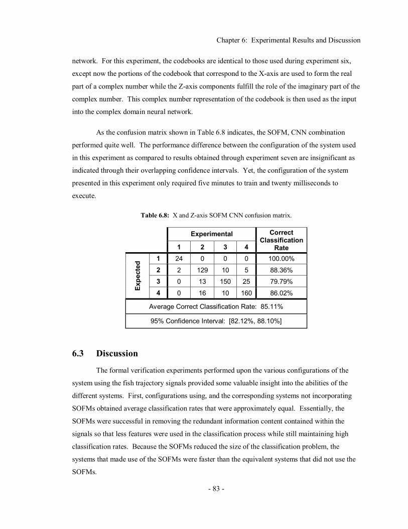
Chapter 6: Experimental Results and Discussion
- 83 -
network. For this experiment, the codebooks are identical to those used during experiment six,
except now the portions of the codebook that correspond to the X-axis are used to form the real
part of a complex number while the Z-axis components fulfill the role of the imaginary part of the
complex number. This complex number representation of the codebook is then used as the input
into the complex domain neural network.
As the confusion matrix shown in Table 6.8 indicates, the SOFM, CNN combination
performed quite well. The performance difference between the configuration of the system used
in this experiment as compared to results obtained through experiment seven are insignificant as
indicated through their overlapping confidence intervals. Yet, the configuration of the system
presented in this experiment only required five minutes to train and twenty milliseconds to
execute.
6.3 Discussion
The formal verification experiments performed upon the various configurations of the
system using the fish trajectory signals provided some valuable insight into the abilities of the
different systems. First, configurations using, and the corresponding systems not incorporating
SOFMs obtained average classification rates that were approximately equal. Essentially, the
SOFMs were successful in removing the redundant information content contained within the
signals so that less features were used in the classification process while still maintaining high
classification rates. Because the SOFMs reduced the size of the classification problem, the
systems that made use of the SOFMs were faster than the equivalent systems that did not use the
SOFMs.
Table 6.8: X and Z-axis SOFM CNN confusion matrix.
Experimental
1 2 3 4
Correct Classification
Rate 1 24 0 0 0 100.00%
2 2 129 10 5 88.36%
3 0 13 150 25 79.79%
Expe
cted
4 0 16 10 160 86.02%
Average Correct Classification Rate: 85.11%
95% Confidence Interval: [82.12%, 88.10%]

Chapter 6: Experimental Results and Discussion
- 84 -
A second general observation that can be made from these experiments is that the
classification systems that made use of only the X-axis information outperformed those systems
which only used the Z-axis information. This indicates that the X-axis contains more important
information than the Z-axis. Configurations that made use of both axes simultaneously, however,
dramatically outperformed the systems that only utilized one axis. Intuitively this finding makes
sense as the clustering techniques as explained in Appendix B use both axes when deriving the
classes. Hence, when a classification system only makes use of one of the X or Z-axis, it is
effectively only taking only half the information content of the signal into account. The systems
making use of both axes used all the information in the signals when making classification
decisions, which provided higher classification rates. In improving the classification rate above
configurations utilizing only a single axis, the neural networks when presented with both axes,
demonstrated that they were also able to differentiate between which axis information was
important when making each individual classification decision. More specifically, the X-axis
seemed to contain the most important information regarding classes one and two while the Z-axis
seemed to provide the most information regarding class four. Both the CNN and PNN were able
to use the complementary information from each of the signals in order to achieve greater
classification accuracy.
A third observation to note is in regard to the training and execution times of the two
neural networks used to perform classification based on the selected features. It was stated in the
background that probabilistic neural networks train orders of magnitude faster than most other
neural networks, and this fact is corroborated by the results of the experiments performed. When
comparing the training time of experiment five to that of experiment seven, the PNN trained more
than 50 times faster than the CNN. In comparing experiments six and eight, the CNN was
approximately 100 times slower than the PNN. In terms of execution time, PNNs were stated to
generally have slower execution times than other neural networks, and again, the experiments
confirmed this fact. In the experiments performed in this thesis, once trained properly, the CNNs
were able to classify input vectors more than eight times faster than the PNNs. But in the end,
both networks were fully able to meet and exceed both of the time design constraints, in that the
training time for the neural networks were only on the order of minutes or seconds, and the
networks were both able to perform classification upon eight separate eight hour signals in less
than a second; hence, based on their speed of execution, they would be applicable for use in real-
time systems.

Chapter 6: Experimental Results and Discussion
- 85 -
Overall, from the experiments it appears that the system used in experiment five whereby
the PNN makes use of both X and Z-axis information provided the highest correct classification
results. This configuration of the system attained an average classification rate of about 90%
which indicates that a high degree of confidence can be placed in the results obtained by the
system. However, one may wonder why the system does not obtain classification rates in the
range of 95-100%, especially when both the clustering analysis and PNN techniques use
Euclidean distance during their calculations. The main flaw in this logic is that the training and
testing sets were derived directly from the fish trajectory time series, whereas the actual
classification system based its decisions upon the multifractal characterization provided by the
variance fractal dimension trajectory. Hence, the clustering analysis performed to derive the
testing and training sets is very sensitive to factors such as changes in magnitude and phase shifts.
Because of these shortcomings with the clustering algorithm, the training and testing sets derived
and used for the formal experiments may not be optimal. These non-ideal testing and training
sets would be a contributing factor in decreasing the average classification rate. Other reasons
why a perfect classification rate is not practical include the fact that the signals used in this thesis
contain inherent noise which was not removed during the preprocessing stage and that not enough
training and testing sets were utilized.
6.4 Summary
This section presented the formal experiments conducted in verifying the classification
system developed for this thesis. In performing these experiments with the fish trajectory signals,
the results were mostly as expected and a number of observations were made. First, it is
detrimental to the classification process to ignore information contained in the signal. Second,
while the use of the SOFM was generally unsuccessful in improving the classification of the
system, it was able to reduce the size of the classification problem while maintaining
approximately the same level of accuracy. The PNN and CNN both performed well; however,
the PNN trained orders of magnitude faster than the CNN, but the CNN executed faster than the
PNN. In the end, all the design constraints for the classification system were met in the particular
configuration where the PNN utilized the VFDT from both the X and Z axes as the features for
classification.

Chapter 7: Conclusions and Recommendations
- 86 -
CHAPTER 7
CONCLUSIONS AND RECOMMENDATIONS
7.1 Conclusions
This thesis illustrated a system capable of classifying the general group of self-similar,
stochastic, non-stationary signals which originated from non-linear processes. This thesis is
unique in that it uses very experimental, but powerful techniques to perform classification upon
these signals, because traditional signal processing methods are insufficient. The use of the
VFDT has also been shown to be effective in extracting a set of compressed features which
represent the characteristics of the signal while simultaneously performing normalization. These
fractal dimension features have been shown to be a sufficient metric upon which to classify these
challenging signals. Furthermore, probabilistic neural networks and complex domain neural
networks have been shown to be capable of performing classification based on these extracted
features with a high degree of success. The system developed for this thesis is also very practical
as it has been designed to adapt to a wide array of signals including those which are composed of
multiple signals.
This thesis presented various different configurations of the classification system. One
system was shown to meet all the specified design criteria, namely a correct classification rate of
at least 90%, a system training time of less than one day, and an execution time of less than the
signal duration itself. Several other configurations also met the time-based constraints, but failed
to meet the correct classification rate by about 5-10%.
7.2 Recommendations
Although the classification system created for this thesis was shown to perform quite
successfully in classifying non-stationary, self-similar, stochastic signals which may or may not
consist of multiple recordings, there are always further improvements that could be made. One
such enhancement would be to tweak the PNN training algorithm that selects a separate sigma
value for each class so that it correctly functions with the fish trajectory signals. Similarly, the
multi-sigma concept could be extended even further to include a separate sigma value for each
variable. This could improve performance in the case where the inputs to the PNN consist of
Chapter 7: Conclusions and Recommendations
- 87 -
multiple recordings as there is no guarantee that each recording has equal importance. A different
sigma for each variable would take the variation of importance of each recording into account and
potentially improve the performance of the PNN with such signals.
Additionally, the classification system could be extended to incorporate hypercomplex
inputs. In the case of the fish trajectory signals, this addition would allow all the axes to be
included in the classification process rather than just the X and Z axes. For the fish trajectory
signal, this addition may not significantly improve performance as it is difficult to gauge the
importance the Y-axis readings. However, other signals that consist of three or more independent
recordings, each of which holds significant information content, may benefit greatly from this
enhancement.
Another beneficial task that could be undertaken is comparing the results of the
classification system developed for this thesis with those derived by expert psychologists
studying the fish trajectory signals. This collaboration was not arranged in time for this thesis,
hence the classes were derived and the system verified in a completely objective manner.
Comparing the objective classification system with the subjective analysis performed by the
experts would provide another metric to evaluate the performance of the system and may lead to
insight as to further improvements to the system
A total of 17 different fish trajectory signals were used for the formal experiment in this
thesis. Of these 17 recordings, nine were used for training while eight where used for testing the
system. These signal recordings provided sufficient results for this thesis, but incorporating a
larger training set should improve the performance of the system and an increased testing set
would provide a better overall picture of the system’s performance.
A task that could be completed to further verify the performance of the system would be
to superimpose synthetic noise upon the signals in order to test the system’s robustness to noise.
Further, the use of additional types of signals with the system would further test the neutrality of
the system with respect to the specific signal used and would show that the system can be applied
to a variety of stochastic, self-similar, non-stationary signals with a high level of success.

References
- 88 -
REFERENCES
[Chen01] J. Chen, Classification of Transients in Power Systems. MSc Thesis, University of
Manitoba, 2001.
[Doug99] B. Douglas, Doing Hard Time: Developing Real-Time Systems with UML, Objects,
Frameworks, and Patterns. Reading, MA: Addison Wesley Longman, Inc., 1999.
[EbDo90] R. Eberhart and R. Dobbins, Neural Network PC Tools: A Practical Guide. San
Diego, CA: Academic Press, Inc., 1990.
[Fere95] K. Ferens, Perceptual Measures off Signal Features. Ph.D. Thesis, University of
Manitoba, 1995.
[Hayk99] S. Haykin, Neural Networks: A Comprehensive Foundation. Upper Saddle River,
NJ: Prentice-Hall, Inc., 1999.
[KaKw92] B.L. Kalman and S.C. Kwasny, “Why tanh? Choosing a sigmoidal function”,
International Joint Conference on Neural Networks, vol. 4, pp. 578-581, June 1992.
[Kins94] W. Kinsner, “Batch and real-time computation of a fractal dimension based on
variance of a time series,” Technical Report, DEL94-6; UofM; June 15, 1994,
(v+17) 22 pp.
[Koho84] T. Kohonen, Self-Organization and Associative Memory. Berlin: Springer-Verlag,
1984.
[Mall98] S. Mallat, A Wavelet Tour of Signal Processing. San Diego, CA: Academic Press,
1998.
[Mand82] B. Mandelbrot, The Fractal Geometry of Nature. San Francisco, CA: W. H.
Freeman and Co., 1982.
[Mast93] T. Masters, Practical Neural Network Recipes in C++. San Diego, CA: Academic
Press, Inc., 1993.
References
- 89 -
[Mast94] T. Masters, Signal and Image Processing with Neural Networks: A C++
Sourcebook. New York, NY: John Wiley & Sons, Inc., 1994.
[Mast95] T. Masters, Advanced Algorithms for Neural Networks: A C++ Sourcebook. New
York, NY: John Wiley & Sons, Inc., 1995.
[Meis72] W. Meisel, Computer-Oriented Approaches to Pattern Recognition. New York, NY:
Academic Press, 1972.
[Parz62] E. Parzen, “On estimation of a probability density function and mode”, Annals of
Mathematical Statistics, 33:3, pp. 1065-1076, 1962.
[PeJS92] H.O. Peitgen, H. Jürgens, and D. Saupe, Chaos and Fractals: New Frontiers of
Science. New York, NY: Springer Verlag, 1992.
[PrFTV88] W. Press, B. Flannery, S. Teukolsky, and W. Vetterling, Numerical Recipes in C.
New York, NY: Cambridge University Press, 1988.
[Spec88] D.F. Specht, “Probabilistic neural networks for classification, mapping, or
associative memory”, IEEE International Conference on Neural Networks, vol. 1,
pp. 525-532, July 1988.
[Spec92] D.F. Specht, “Enhancements to probabilistic neural networks”, International Joint
Conference on Neural Networks, vol. 1, pp. 761-768, June 1992.
[Wass93] P. Wasserman, Advanced Methods in Neural Computing. New York, NY: Van
Nostrand Reinhold, 1993.
[WeKu91] S. Weiss and C. Kulikowski, Computer Systems that Learn: Classification and
Prediction Methods from Statistics, Neural Nets, Machine Learning, and Expert
Systems. San Mateo, CA: Morgan Kaufmann Publishers, Inc., 1991.
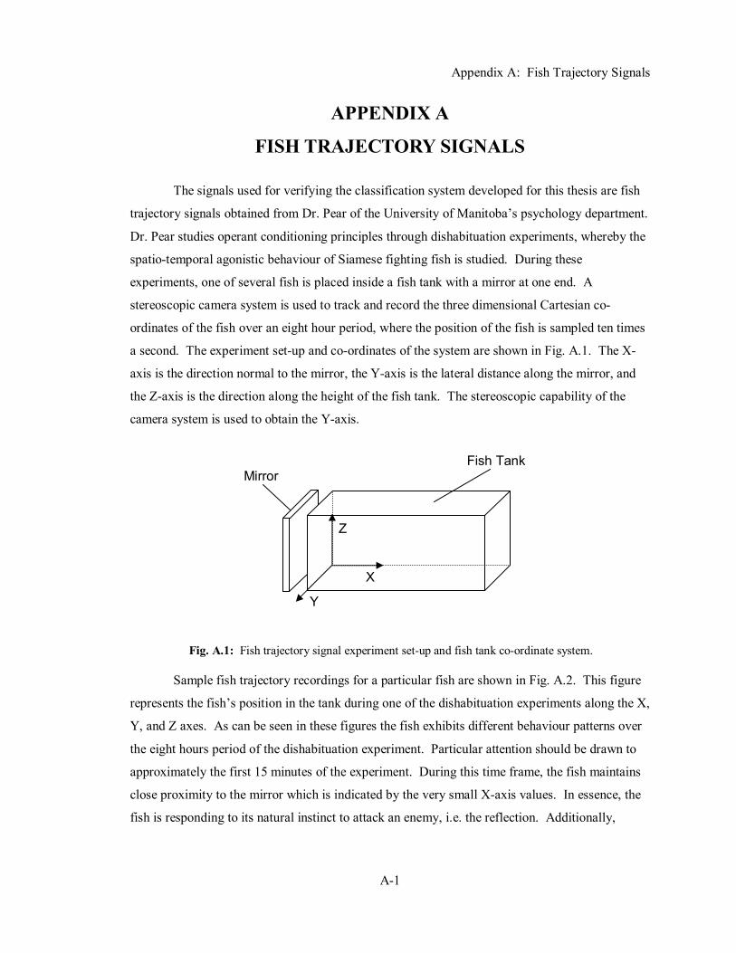
Appendix A: Fish Trajectory Signals
A-1
APPENDIX A
FISH TRAJECTORY SIGNALS
The signals used for verifying the classification system developed for this thesis are fish
trajectory signals obtained from Dr. Pear of the University of Manitoba’s psychology department.
Dr. Pear studies operant conditioning principles through dishabituation experiments, whereby the
spatio-temporal agonistic behaviour of Siamese fighting fish is studied. During these
experiments, one of several fish is placed inside a fish tank with a mirror at one end. A
stereoscopic camera system is used to track and record the three dimensional Cartesian co-
ordinates of the fish over an eight hour period, where the position of the fish is sampled ten times
a second. The experiment set-up and co-ordinates of the system are shown in Fig. A.1. The X-
axis is the direction normal to the mirror, the Y-axis is the lateral distance along the mirror, and
the Z-axis is the direction along the height of the fish tank. The stereoscopic capability of the
camera system is used to obtain the Y-axis.
Sample fish trajectory recordings for a particular fish are shown in Fig. A.2. This figure
represents the fish’s position in the tank during one of the dishabituation experiments along the X,
Y, and Z axes. As can be seen in these figures the fish exhibits different behaviour patterns over
the eight hours period of the dishabituation experiment. Particular attention should be drawn to
approximately the first 15 minutes of the experiment. During this time frame, the fish maintains
close proximity to the mirror which is indicated by the very small X-axis values. In essence, the
fish is responding to its natural instinct to attack an enemy, i.e. the reflection. Additionally,
Fig. A.1: Fish trajectory signal experiment set-up and fish tank co-ordinate system.
X
Z
Y
Fish Tank Mirror

Appendix A: Fish Trajectory Signals
A-2
Fig. A.2: Fish trajectory signals.

Appendix A: Fish Trajectory Signals
A-3
during these initial 15 minutes the fish remains close to the surface of the tank, as indicated by
large Z-axis values. This behaviour is exhibited because the fish breathes air and requires more
air when it is excited.
Following the initial 15 minute period the fish begins to move farther away from the
mirror and for longer periods of time. At seven hours into the experiment, the mirror is removed
for 60 seconds and a dishabituation stimulus is presented in an attempt to have the fish revert to
its initial behaviour. This dishabituation stimulus is a conspecific – another Siamese fighting fish
– in a separate fish tank positioned at the side of the tank directly opposite the mirror. After 60
seconds the mirror is restored to its original position and the conspecific is removed.
As previously mentioned, the stereoscopic portion of the camera system was used to
obtain the Y-axis recordings. Because of this configuration, the Y-axis is the least accurate of
any of the axes. This was arranged because the Y-axis is the only direction which there is no
explicit stimuli and is considered the least significant in terms of the information provided. Both
the mirror and conspecific are stimuli along the X-axis and is correspondingly considered the axis
that contains the most useful information. While the experiment presents no stimuli along the Z-
axis, what differentiates this direction from that of the Y-axis is that the fish must periodically
breathe air, and this action of rising to the surface of the water to breathe has significance in the
experiment. As this thesis restricts its scope to developing a system to classify signals composed
of two correlated recordings, only the X and Z axes used for the purpose of verifying the system.
As with all real signals, the tracking system is subject to noise and inaccuracies along all
three axes. Furthermore, because of the set-up of the experiment, the system sometimes
encounters tracking errors where the fish moves into a particular position close to the mirror that
is outside the view of the camera, and results in missing samples. These non-idealities aid in
testing the robustness of the signal classification system.
An important issue to consider when processing any signal is the sampling rate.
Obviously the sampling rate must adhere to the Nyquist sampling theorem. The following
explanation justifies the sampling rate used in the recording of the fish trajectory signals. Assume
that the fish moves in a sinusoidal trajectory at the Nyquist frequency, or half of the sampling
frequency. Further, assume that the amplitude of the sinusoidal is approximately the size of the
fish, since this guarantees that the tracking system identifies this lateral motion. The resulting
signal is given by x = Asinωt, where A is the amplitude, 2 cm, and ω is the Nyquist frequency,

Appendix A: Fish Trajectory Signals
A-4
2π5 rad/s. The corresponding velocity is given by the derivative of this sinusoidal, v = Aωcosωt.
If the fish is to travel this particular trajectory, then it must be able to move at the maximum
velocity, Aω. Thus, the fish must be able to reach a speed of 62.8 cm/s. However, this value is
beyond the maximum speed of the fish observed during these experiments and thus, it is not
possible for there to be frequencies above the Nyquist frequency, given the sampling rate of 10
Hz. Therefore, the sampling rate is valid for this signal.
The purpose of attempting signal classification upon these signals is to identify the
various behaviours exhibited by the fish in an automated, quantitative manner. This quantitative
assessment based on the position of the fish in the fish tank could then be compared to the
psychological qualitative analysis performed by Dr. Pear and his graduate students. Because this
signal emanates from a living being that is acting erratically, the system in question is non-linear.
Further, the fish’s reaction to the stimuli is random in nature and changes over time, hence its
stochastic and non-stationary properties. The self-similarity property of a signal is difficult to
intuitively identify, but it can be shown that the signal is indeed self-similar. Because of the
complex nature of the signal and the properties it exhibits, this fish trajectory signal is used as the
basis to verify the performance of the classification system developed for this thesis.

Appendix B: Clustering of Fish Trajectory Signals
B-1
APPENDIX B
CLUSTERING OF FISH TRAJECTORY SIGNALS
The fish trajectory signals used for the verification of the classification system developed
for this thesis were not accompanied by the specification of the classes. However, example
signals from each of the different classes are required in order to establish the training and testing
sets. For the purposes of this thesis, the determination of the classes is to be performed in an
objective manner that is unbiased with respect to the techniques used in the thesis itself.
Furthermore, this class specification is to be performed assuming nothing about the data itself, so
as not to bias the results based on a priori information.
In order to determine these class specifications, it is desired to perform a clustering
analysis upon the signals to discover the groupings that exist within the signal. There are
numerous techniques for performing clustering, but most require that at minimum, the number of
classes be known a priori; information that is unfortunately not known for the fish trajectory
signals. The proposed clustering technique is Kohonen self-organizing feature maps (SOFMs), as
discussed in the background in Chapter 2. This unsupervised neural network is able to perform a
topology-preserving clustering with no a priori information about the data. The result of training
the network is a codebook consisting of codewords representative of the input vectors to be
clustered. The codewords in the codebook are grouped in the codebook based on their similarity.
By visually viewing the groupings of the codewords, the underlying clustering of the signal can
be inferred.
Each signal is divided up into a number of segments and it is these segments of the
signals which are to be classified by the system and thus clustering is based upon these segments.
By utilizing these segments of the signal as the input vectors to the SOFM, it will produce the
desired codebook containing the clusters. However, it would be naïve to perform clustering only
upon one axis since it would then completely ignore the information contained in the other axes.
Since this thesis restricts the classification to complex valued signals composed of two separate
recordings and the purpose of utilizing these fish trajectory signals is solely for the verification of
the system, not the analysis of the behaviours of the fish, only the axes considered to be the most
important, the X and Z-axis, are considered. In order to adapt the SOFM to perform clustering by
taking both axes into account, the input vectors to the SOFM are formed by concatenating the
signal segments from the X and Z-axis, as explained in Eq. (3.1).
Appendix B: Clustering of Fish Trajectory Signals
B-2
The difficulty in performing this clustering based on both the X and Z-axis is that
because of the nature of the signals, the fish exhibits more dramatic changes along the X-axis as
compared to the Z-axis. This inequity causes a problem because the X-axis influences the
clustering much more than the Z-axis because of its greater changes in magnitude. To circumvent
this problem and to put the two axes on equal footing, a Z-score normalization is performed
separately upon the axes, whereby the signal samples are normalized according to (B.1), where x
is the sample, x is the sample mean of all the samples for the axis, and s is the sample standard
deviation of all the samples for the axis.
x xy
s−
= (B.1)
The axes are separately normalized such that the mean of all the samples for the axis is zero and
the standard deviation is one. This normalization ensures that both axes equally influence the
outcome of the clustering, as desired. This need for explicit normalization is in contrast to the
actual classification system where the computed variance fractal dimension trajectory naturally
produces normalized features.
The details of the operation and training of the network, as well as the design,
implementation, and testing and verification of the SOFM can be found in the body of the thesis.
Once the SOFM has been trained, the codebook must then be analyzed to discover the
clusters of the signal segments. It was found that segments of length 4096 samples, or
approximately 6.8 minutes, produced decent clustering. Plots of the codebook using segments of
the aforementioned size are shown in Fig. B.1 where the portions of the codewords corresponding
to the different axes are first extracted and then appended together. Thus, in the figure, the first
codeword actually consists of the segment between 0 and 1 of the X-axis codebook followed by a
concatenation of the segment between 0 and 1 of the Z-axis codebook. Note that visually, the
codewords are grouped together in such a manner that adjacent codewords are similar.
There is a range of segment lengths where the clustering yields similar results. It was
discovered that, lengths between 2048 and 4096 samples produced similar codebooks, meaning
that the classes of the signal are approximately constant over 4096 samples. Here, the segment
size selected was the largest segment where the signal’s class of behaviour remained constant, i.e.
4096 samples.
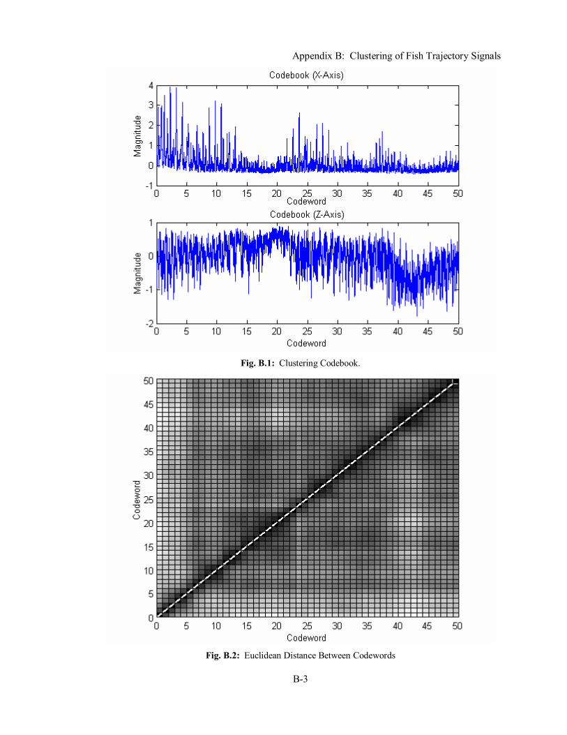
Appendix B: Clustering of Fish Trajectory Signals
B-3
Fig. B.1: Clustering Codebook.
Fig. B.2: Euclidean Distance Between Codewords

Appendix B: Clustering of Fish Trajectory Signals
B-4
Direct analysis of the clustering in this view is quite difficult. In order to better view the
clustering, a plot is created to exemplify the relative similarity between the codewords. The
judge of similarity between codewords is done by computing the Euclidean distance between all
the combinations of codewords and plotting these results in a colour map, as seen in Fig. B.2.
The number of the codewords appears along both axes and the value for a given row and column
is the Euclidean distance between the two codewords. The distance between two codewords is
represented in the figure as a gray scale colouring, where black corresponds to a distance of zero
and white corresponds to a very high distance. Note that the values along the diagonal should
always be black because the distance between a codeword and itself is zero. The fact that the
diagonal appears to be white in the figure is merely an artifact of the plotting program used. The
groupings can be much more easily seen in this plot because the relative similarity of the
codewords is clearly shown. Dark sections are indicative of groups of codewords that can be
considered to be of the same class. Ideally, if the groupings were very distinct and separable,
there would be several dark areas where the intersection of the dark areas on the map are lightly
coloured, meaning that none of the codewords in a particular class are similar to the codewords in
any other class.
This plot shows some separability of the classes, but it is difficult to see in print. There
seems to be a distinct class consisting of the codewords 0 through 5, as the Euclidean distance
between all these codewords are very small, and the Euclidean distance between these codewords
and others are substantially higher. The second class appears to be between 6 and 22, but are not
as well formed as the first class. There appears to be a third class between the 23rd and 39th
codewords, which leaves the codewords from 40 to 49 as the fourth class. Referring back to Fig.
B.1, these classes seem reasonable, as the codewords defined to be of the same class visually
seem similar. By identifying these clusters, the signals can be annotated by segmenting them into
lengths of 4096, which corresponds to the codeword size and discovering to which codeword it
corresponds. The codeword corresponding to a given signal segment is determined by the
“winner” neuron in the SOFM for that given input. The class which that codeword belongs, as
determined by the visual inspection, is then assigned to the signal segment in question. This
procedure is repeated for every segment in each signal. These segments now act as examples for
each of the classes for use in the formation of training and testing tests. With segments of size
4096 samples, there are 68 segments in each signal. The segments in nine of the files are set
aside for the training set and the segments in the other eight files are set aside for the testing set.

Appendix B: Clustering of Fish Trajectory Signals
B-5
Note that this clustering is based on the time domain, so it is sensitive to changes in such
things as magnitude and phase shifts. The simple similarity of signals when compared sample to
sample is not a particularly good judgement of whether the signals have the same behaviour and
hence, belong to the same class, but it is an objective way of performing this clustering and is
unbiased to the techniques used in this thesis.

Appendix C: Source Code
C-1
APPENDIX C
SOURCE CODE
The source code for all of the programs written for the various configurations of the
classification system developed for this thesis is provided on the attached CD. The source code
can be found the “src” directory. In addition to the source code, full documentation in the form of
Javadocs for all of the programs is supplied on the CD in the “doc” directory.

CONTRIBUTIONS
Thesis Report
The writing of this thesis was a combined effort between the two team members.
Although the entire thesis was edited and revised by both group members, the following list
indicates which individual made substantial written contributions to each section of the report.
Abstract ............................................................................... [Kevin and Vincent]
Chapter 1 Introduction....................................................... [Kevin and Vincent]
Chapter 2 Background 2.1 Signal Classification and Terminology ............................................................ [Kevin] 2.2 Fractals ................................................................................................................ [Kevin]
2.2.1 Introduction ............................................................................................. [Kevin] 2.2.2 Variance Fractal Dimension ..................................................................... [Kevin]
2.3 Neural Networks ...............................................................................[Kevin and Vincent] 2.3.1 Introduction ............................................................................................. [Kevin] 2.3.2 Basic Concepts ........................................................................................ [Kevin] 2.3.3 Backpropagation ...................................................................................... [Kevin] 2.3.4 Complex Domain Neural Networks....................................................... [Vincent] 2.3.5 Probabilistic Neural Networks.................................................................. [Kevin] 2.3.6 Kohonen Self-Organizing Feature Maps................................................ [Vincent]
Chapter 3 System Design 3.1 System Architecture .......................................................................................... [Vincent] 3.2 Component Design ............................................................................................ [Vincent]
3.2.1 Preprocessing........................................................................................ [Vincent] 3.2.2 Variance Fractal Dimension Trajectory ................................................. [Vincent] 3.2.3 Kohonen Self-Organizing Feature Map ................................................. [Vincent] 3.2.4 Probabilistic Neural Network ................................................[Kevin and Vincent] 3.2.5 Complex Domain Neural Network ........................................................ [Vincent]
Chapter 4 System Implementation ..................................................[Vincent]
Chapter 5 System Verification and Testing....................... [Kevin and Vincent]
Chapter 6 Experimental Results and Discussion .............. [Kevin and Vincent]
Chapter 7 Conclusions and Recommendations ................. [Kevin and Vincent]
Appendix A Fish Trajectory Signals.................................. [Kevin and Vincent]
Appendix B Clustering of Fish Trajectory Signals .........................[Vincent]

Individual Contributions
Individual Work Completed Kevin Cannons Implemented Brent’s line minimization algorithm.
Implemented the conjugate gradient multi-sigma training algorithm for the PNN. Extensively tested and compared the performance of the single sigma PNN and the multi-sigma PNN.
Vincent Cheung Designed and implemented the preprocessing, variance fractal dimension trajectory, Kohonen self-organizing feature map, probabilistic neural network, and complex domain neural network components. Designed and implemented the classes to create the input vectors for classification and for performing the actual classification of the signals with the various configurations of the system. Thoroughly tested and verified each component as well as the overall system. Optimized the VFDT, SOFM, PNN, and CNN parameters. Conducted the formal verification experiments to compare the performance of the various configurations of the system with the fish trajectory signals. Performed the clustering of the fish trajectory signals using Kohonen self-organizing feature maps in order to develop the training and testing sets.

VITA
NAME: Kevin Cannons
PLACE OF BIRTH: Palo Alto, California, USA
YEAR OF BIRTH: 1981
SECONDARY Shaftesbury High School EDUCATION:
HONOURS and 1999 AWARDS: • Advanced Placement and International Baccalaureate
Scholarship Enhancement • APEGM Engineering Entrance Scholarship • Dr. Kwan Chi Kao Entrance Scholarship in Engineering • I.O.D.E Jon Sigurdsson Memorial Entrance Scholarship • University of Manitoba Advanced Early Admission
Scholarship 2000-2002
• Dean’s Honour List • UMSU Scholarship
2000
• Faculty of Engineering Second Year Scholarship • NSERC Undergraduate Student Research Award
2001
• Engineering Academic Excellence Award • Grettir Eggertson Memorial Scholarship • Technical Communication Report Prize
2002
• Grettir Eggertson Memorial Scholarship • NSERC Undergraduate Student Research Award

VITA
NAME: Vincent Cheung
PLACE OF BIRTH: Thompson, Manitoba, Canada
YEAR OF BIRTH: 1981
SECONDARY Shaftesbury High School EDUCATION:
HONOURS and 1999 AWARDS: • Governor General’s Award
• Advanced Placement and International Baccalaureate Scholarship Enhancement
• APEGM Engineering Entrance Scholarship • Challenge Math Award • Doug Strang Memorial / Reid Crowther Scholarship • Dr. Kwan Chi Kao Scholarship • Johana Gudrun Skaptason Scholarship • Manitoba Hydro Entrance Scholarship
2000-2002
• Dean’s Honour List • Dr. A.W. Hogg Undergraduate Scholarship • Isbister Scholarship in Engineering • MTS Pursue Your Calling Scholarship • UMSU Scholarship
2000
• APEGM First Year Scholarship • Dr. Kwan Chi Kao Scholarship in Elec. and Comp. Eng. • Edward Oliver Grimsdick Memorial Prize • EECOL Electric Inc. Scholarship • Faculty of Engineering Second Year Scholarship
2001
• Donald George Lougheed Memorial Scholarship • Engineering Academic Excellence Award - Comp. Eng. • Royal Air Force Auxiliary Memorial Scholarship • Technical Communication Report Prize
2002
• Abitibi-Consolidated Inc. Scholarship • Dr. Kwan Chi Kao Scholarship in Computer Engineering • NSERC Undergraduate Student Research Award