Simulating the Dow Jones Industrial Average: A Further Test of the Random Walk Hypothesis

CFA Institute

Simulating the Dow Jones Industrial Average: A Further Test of the Random WalkHypothesisAuthor(s): Edward F. Renshaw and Vernon D. RenshawSource: Financial Analysts Journal, Vol. 26, No. 5 (Sep. - Oct., 1970), pp. 51-59Published by: CFA InstituteStable URL: http://www.jstor.org/stable/4470725 .

Accessed: 15/06/2014 00:48

Your use of the JSTOR archive indicates your acceptance of the Terms & Conditions of Use, available at .http://www.jstor.org/page/info/about/policies/terms.jsp

.JSTOR is a not-for-profit service that helps scholars, researchers, and students discover, use, and build upon a wide range ofcontent in a trusted digital archive. We use information technology and tools to increase productivity and facilitate new formsof scholarship. For more information about JSTOR, please contact [email protected].

.

CFA Institute is collaborating with JSTOR to digitize, preserve and extend access to Financial AnalystsJournal.

http://www.jstor.org

This content downloaded from 91.229.229.44 on Sun, 15 Jun 2014 00:48:51 AMAll use subject to JSTOR Terms and Conditions

http://www.jstor.org/action/showPublisher?publisherCode=cfa

http://www.jstor.org/stable/4470725?origin=JSTOR-pdf

http://www.jstor.org/page/info/about/policies/terms.jsp


Simulating the Dow Jones

Industrial Average:

A further test of the

Random Walk Hypothesis

by Edward F. and Vernon D. Renshaw

W HILE both of IBM's portfolio selection programs were developed on the assumption that subjective estimates, of relevant parameters might

be useful in obtaining efficient portfolios, the usefulness of subjective estimates has never been demonstrated to the best of our knowledge. In the meantime, however, evidence has accumulated to suggest that there may be some degree of predictive content to the parameters that are obtained from historical data. [ 16] Studies by Smith [ 12 ], [ 13 ], and Cohen and Pogue [2] have used varia- tions of the Sharpe-Markowitz programs [6], [7], [11] to obtain portfolios from historical data which have performed so well in subsequent periods as to possibly be inconsistent with the random walk hypothesis.

In this article we will use some simplified portfolio balance models to obtain a reasonably efficient portfolio for the Dow Jones Industrial Average (DJIA) in the period 1947-65. The resulting portfolios will then be compared to some simulated portfolios which were derived on the basis of a model suggested by M. F. M. Osborne. Our main conclusion is that distributions of stock re-turns which appear to conform to the laws of

random motion can hide a significant amount of internal structure.

The fairly stable risk parameters observed for the stocks in the DJIA suggest that portfolio balance models can be used to identify securities which will be significantly more defensive in future periods than a representative price index. The bear markets of 1966 and 1969 help to confirm this hypothesis. The simplified portfolios obtained for the period 1947-65 were not only more defensive than the DJIA in these markets but also turned out to be superior to other portfolios which are pre- sumed to be defensive, such as those stocks with the least average variance.

If investors are aware of this structure and endeavor to get out of defensive stocks during bull markets and to move back into efficient portfolios when the outlook becomes more bearish, this would tend to reinforce the parameter structure observed for the DJIA and make arbitrage even more worthwhile. A detailed analysis of risk parameters, in other words, might increase the in- stability of some stock prices and possibly the market in general, if fluctuations in the economy are not exactly random.

Simulating the Dow Jones Industrial Average

In his now classic article on "Brownian Motion in the Stock Market," Osborne has suggested that logarithmic changes in stock prices can be expressed as the sum of two variables, where the first variable is common to all stocks at a given time and the second variable is independent for each stock. Our method of simulating the

[ ] References appear at end of article.

EDWARD F. RENSHAW is Professor of Economics and Finance, State University of New York at Albany.

VERNON D. RENSHAW is presently a Ph.D. candidate, the Department of Economics at Massachusetts Institute of Technology.

FINANCIAL ANALYSTS JOURNAL / SEPTEMBER-OCTOBER 1970 51



Dow Jones Industrial Average is essentially equivalent to Osborne's Model II [3, p. 113], where:

rt = the annual percentage return including dividends for an individual security,

At-the annual percentage return including dividends on Standard & Poor's (S&P's) composite stock index, and

ut a random deviate which has been drawn from a log normal distribution with a standard deviation of 20 percentage points:

we can link the partly random returns on an individual security to the market average in the following way:

rt At + ut. (1)

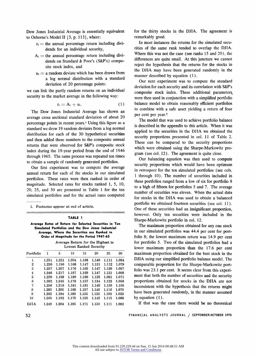
The Dow Jones Industrial Average has shown an average cross sectional standard deviation of about 20 percentage points in recent years.' Using this figure as a standard we drew 19 random deviates from a log normal distribution for each of the 30 hypothetical securities and then added these numbers to the composite annual returns that were observed for S&P's composite stock index during the 19-year period from the end of 1946 through 1965. The same process was repeated ten times to obtain a sample of randomly generated portfolios.

Our first experiment was to compute the average annual return for each of the stocks in our simulated portfolios. These rates were then ranked in order of magnitude. Selected rates for stocks ranked 1, 5, 10, 20, 25, and 30 are presented in Table 1 for the ten simulated portfolios and for the actual rates computed

for the thirty stocks in the DJIA. The agreement is remarkably good.

In most instances the returns for the simulated securities of the same rank tended to overlap the DJIA. Where this was not the case (see ranks 15 and 20), the differences are quite small. At this juncture we cannot reject the hypothesis that the returns for the stocks in the DJIA may have been generated randomly in the manner described by equation (1).

Our next experiment was to compute the standard deviation for each security and its correlation with S&P's composite stock index. These additional parameters, were then used in conjunction with a simplified portfolio balance model to obtain reasonably efficient portfolios to combine with a safe asset yielding a return of four per cent per year.2

The model that was used to achieve portfolio balance is described in the appendix to this article. When it was applied to the securities in the DJIA we obtained the security proportions presented in col. 11 of Table 2. These can be compared to the security proportions which were obtained using the Sharpe-Markowitz program (see col. 12). The agreement is quite close.

Our balancing equation was then used to compute security proportions which would have been optimum in retrospect for the ten simulated portfolios (see cols. 1 through 10). The number of securities included in these portfolios ranged from a low of six for portfolio 8 to a high of fifteen for portfolios 5 and 7. The average number of securities was eleven. When the actual data for stocks in the DJIA was used to obtain a balanced portfolio we obtained fourteien securities (see col. 11). One of these securities had an insignificant proportion, however. Only ten securities were included in the Sharpe-Markowitz portfolio in col. 12.

The maximum proportion obtained for any one stock in our simulated portfolios was 44.4 per cent for portfolio 8; the lowest maximum return was 14.9 per cent for portfolio 5. Two of the simulated portfolios had a lower maximum proportion than the 17.6 per cent maximum proportion obtained for the best stock in the DJIA using our simplified portfolio balance model. The comparable proportion for the Sharpe-Markowitz portfolio was 23.1 per cent. It seems clear from this experiment that both the number of securities and the security proportions obtained for stocks in the DJIA are not inconsistent with the hypothesis that the returns might have been generated randomly, in the manner assumed by equation ( 1) .

If that was the case there would be no theoretical

TABLE 1

Average Rates of Return for Selected Securities in Ten Simulated Portfolios and the Dow Jones Industrial

Average, Where the Securities are Ranked in Order of Magnitude for the Period 1947-65

Average Return for the Highest to Lowest Ranked Security

Portfolio 1 5 10 15 20 25 30

1 1.251 1.221 1.204 1.168 1.140 1.111 1.094 2 1.236 1.196 1.168 1.147 1.131 1.112 1.079 3 1.257 1.207 1.176 1.165 1.147 1.129 1.097 4 1.246 1.217 1.187 1.169 1.147 1.121 1.098 5 1.220 1.199 1.180 1.160 1.135 1.081 1.071 6 1.282 1.245 1.179 1.157 1.134 1.123 1.058 7 1.256 1.216 1.181 1.161 1.145 1.130 1.105 8 1.285 1.205 1.168 1.157 1.140 1.116 1.070 9 1.262 1.194 1.180 1.155 1.135 1.103 1.033

10 1.265 1.192 1.175 1.155 1.142 1.115 1.088

DJIA 1.249 1.204 1.185 1.171 1.150 1.111 1.092

1. Footnotes appear at end of article.

52 FINANCIAL, ANALYSTS JOURNAL / SEPTEMBER-OCTOBER 197G



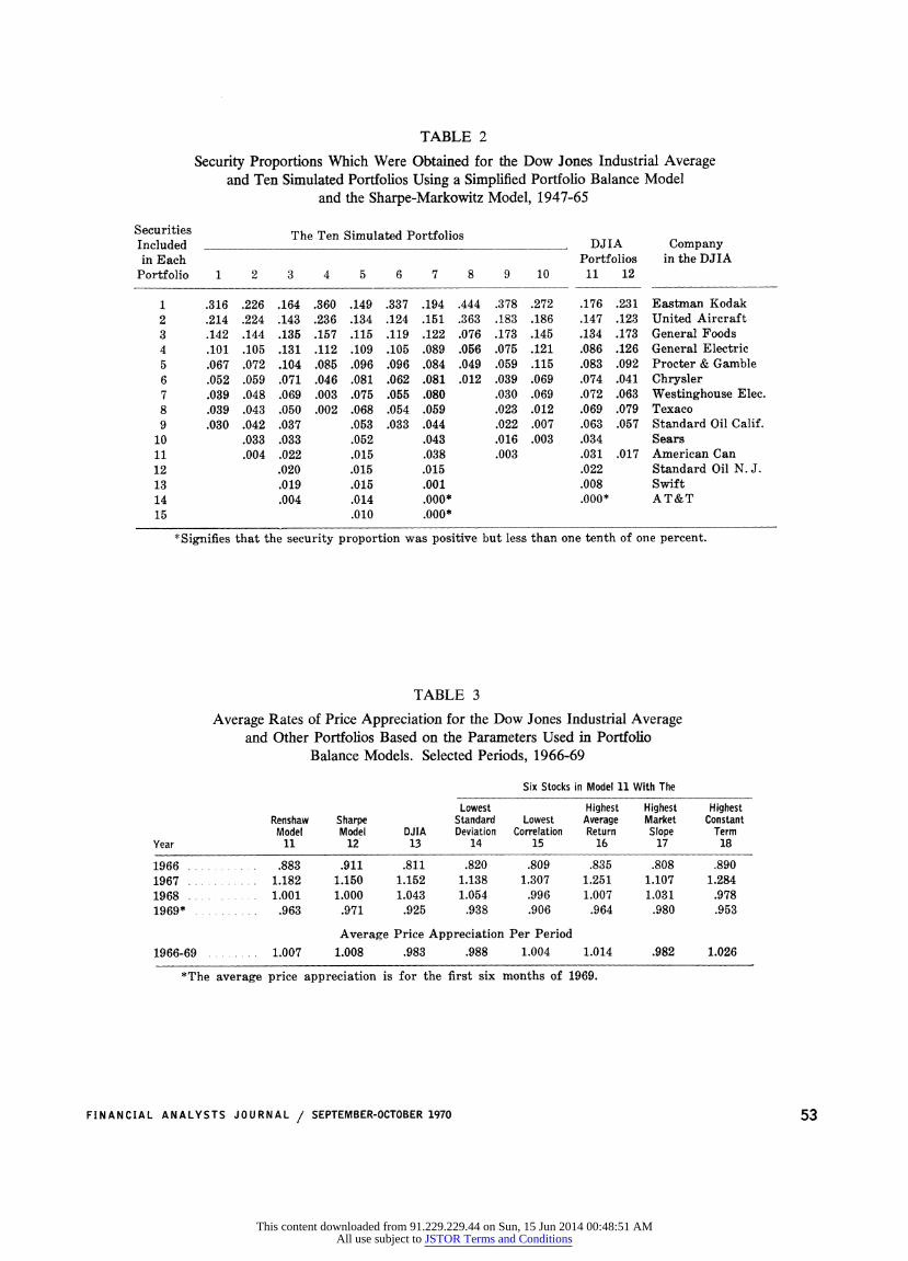
TABLE 2

Security Proportions Which Were Obtained for the Dow Jones Industrial Average and Ten Simulated Portfolios Using a Simplified Portfolio Balance Model

and the Sharpe-Markowitz Model, 1947-65

Securities The Ten Simulated Portfolios DJIA Company Included DJIA___ _ __ _ __ _ _Company__ _ __ _ __ _ __ _

in Each Portfolios in the DJIA Portfolio 1 2 3 4 5 6 7 8 9 10 11 12

1 .316 .226 .164 .360 .149 .337 .194 .444 .378 .272 .176 .231 Eastman Kodak 2 .214 .224 .143 .236 .134 .124 .151 .363 .183 .186 .147 .123 United Aircraft 3 .142 .144 .135 .157 .115 .119 .122 .076 .173 .145 .134 .173 General Foods 4 .101 .105 .131 .112 .109 .105 .089 .056 .075 .121 .086 .126 General Electric 5 .067 .072 .104 .085 .096 .096 .084 .049 .059 .115 .083 .092 Procter & Gamble 6 .052 .059 .071 .046 .081 .062 .081 .012 .039 .069 .074 .041 Chrysler 7 .039 .048 .069 .003 .075 .055 .080 .030 .069 .072 .063 Westinghouse Elec. 8 .039 .043 .050 .002 .068 .054 .059 .023 .012 .069 .079 Texaco 9 .030 .042 .037 .053 .033 .044 .022 .007 .063 .057 Standard Oil Calif.

10 .033 .033 .052 .043 .016 .003 .034 Sears 11 .004 .022 .015 .038 .003 .031 .017 American Can 12 .020 .015 .015 .022 Standard Oil N. J. 13 .019 .015 .001 .008 Swift 14 .004 .014 .000* .000* AT&T 15 .010 .000*

*Signifies that the security proportion was positive but less than one tenth of one percent.

TABLE 3

Average Rates of Price Appreciation for the Dow Jones Industrial Average and Other Portfolios Based on the Parameters Used in Portfolio

Balance Models. Selected Periods, 1966-69

Six Stocks in Model 11 With The

Lowest Highest Highest Highest Renshaw Sharpe Standard Lowest Average Market Constant Model Model DJIA Deviation Correlation Return Slope Term

Year 11 12 13 14 15 16 17 18

1966 ...... .883 .911 .811 .820 .809 .835 .808 .890

1967 . . 1.182 1.150 1.152 1.138 1.307 1.251 1.107 1.284 1968 .1. 1.001 1.000 1.043 1.054 .996 1.007 1.031 .978 1969* .......... .963 .971 .925 .938 .906 .964 .980 .953

Average Price Appreciation Per Period

1966-69 .. . 1.007 1.008 .983 .988 1.004 1.014 .982 1.026

*The average price appreciation is for the first six months of 1969.




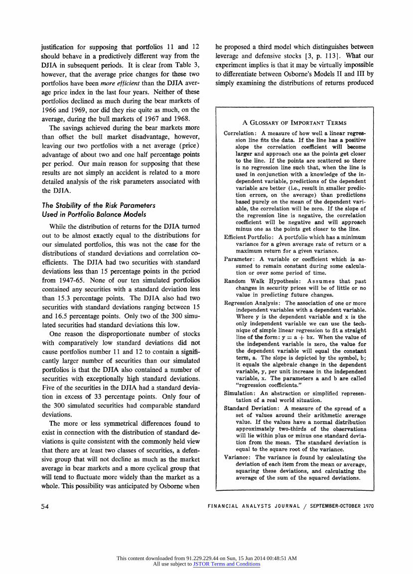
justification for supposing that portfolios 11 and 12 should behave in a predictively different way from the DJIA in subsequent periods. It is clear from Table 3, however, that the average price changes for these two portfolios have been more efficient than the DJIA average price index in the last four years. Neither of these portfolios declined as much during the bear markets of 1966 and 1969, nor did they rise quite as much, on the average, during the bull markets of 1967 and 1968.

The savings achieved during the bear markets more than offset the bull market disadvantage, however, leaving our two portfolios with a net average (price) advantage of about two and one half percentage points per periord. Our main reason for supposing that these results are not simply an accident is related to a more detailed analysis of the risk parameters associated with the DJIA.

The Stability of the Risk Parameters Used in Portfolio Balance Models

While the distribution of returns for the DJIA turned out to be almost exactly equal to the distributions for our simulated portfolios, this was not the case for the distributions of standard deviations and correlation coefficients. The DJIA had two securities with-standard deviations less than 15 percentage points in the period from 1947-65. None of our ten simulated portfolios contained any securities with a standard deviation less than 15.3 percentage points. The DJIA also had two securities with standard deviations ranging between 15 and 16.5 percentage points. Only two of the 300 simulated securities had standard deviations this low.

One reason the disproportionate number of stocks with comparatively low standard deviations did not cause portfolios number 11 and 12 to contain a significantly larger number of securities than our simulated portfolios is that the DJIA also contained a number of securities with exceptionally high standard deviations. Five of the securities in the DJIA had a standard deviation in excess of 33 percentage points. Only four of the 300 simulated securities had comparable standard deviations.

The more or less symmetrical differences found to exist in connection with the distribution of standard deviations is quite consistent with the commonly held view that there are at least two classes of securities, a defensive group that will not decline as much as the market average in bear markets and a more cyclical group that will tend to fluctuate more widely than the market as a whole. This possibility was anticipated by Osborne when

he proposed a third model which distinguishes between leverage and defensive stocks [3, p. 1131. What our experiment implies is that it may be virtually impossible to differentiate between Osbome's Models II and Ill by simply examining the distributions of returns produced

A GLOSSARY OF IMPORTANT TERMS

Correlation: A measure of how well a linear regression line fits the data. If the line has a positive slope the correlation coefficient will become larger and approach one as the points get closer to the line. If the points are scattered so there is no regression line such that, when the line is used in conjunction with a knowledge of the independent variable, predictions of the dependent variable are beitter (i.e., result in, smaller predic- tion errors, on the average) than predictions based purely on the mean of the dependent variable, the correlation will be zero. If the slope of the regression line is negative, the correlation coefficient will be negative and will approach minus one as the points get closer to the line.

Efficient Portfolio: A portfolio which has a minimum variance for a given average rate of return or a maximum return for a given variance.

Parameter: A variable or coefficient which is assumed to remain constant during some calcula- tion or over some period of time.

Random Walk Hypothesis: Assumes that past changes in security prices will be of little or no value in predicting future changes.

Regression Analysis: The association of one or more independent variables with a dependent variable. Where y is the dependent variable and x is the only independent variable we can use the tech- nique of simple linear regression to fit a straight line of the form: y = a + bx. When the value of the independent variable is zero, the value for the dependent variable will equal the constant term, a. The slope is depicted by the symbol, b; it equals the algebraic change in the dependent variable, y, per unit increase in the independent variable, x. The parameters a and b are called "regression coefficients."

Simulation: An abstraction or simplified represen- tation of a real world situation.

Standard Deviation: A measure of the spread of a set of values around their arithmetic average value. If the values have a normal distribution approximately two-thirds of the observations. will lie within plus or minus one standard deviation from the mean. The standard deviation is equal to the square root of the variance.

Variance: The variance is found by calculating the deviation of each item from the mean or average, squaring these deviations, and calculating the average of the sum of the squared deviations.

54 FINANCIAL ANALYSTS JOURNAL / SEPTEMBER-OCTOBER 1970



in the market place. These distributions can apparently hide a great deal of internal structure.

Further evidence of structure is provided by the distribution of correlation coefficients. Eight stocks in the DJIA had a correlation with S&P's composite stock index greater than 80 per cent. None of the simulated portfolios had more than two stocks with an index correlation this high. Four of the simulated portfolios had no stock with a correlation coefficient greater than 0.8.

These differences were also counterbalanced by off- setting differences at the other end of the distribution. The DJIA had six stocks with a correlation less than 0.4. None of the simulated portfolios had more than three stocks with an index correlation this low and three of the portfolios had no stock with a correlation below 0.4.

Another interesting phenomenon to observe in connection with the risk parameter distributions is the tendency for the differences in standard deviations and correlation coefficients to reinforce each other. Most of the stocks in the DJIA with a high correlation coefficient also had very high standard deviations. While those stocks with low correlation coefficients also tended to have low standard deviations, there were a few dramatic exceptions. Chrysler Corporation not only had the lowest index correlation during this period, but also had the highest standard deviation for any company in the DJIA. United Aircraft Company was a similar exception.

The notion that there is structure to the risk param-

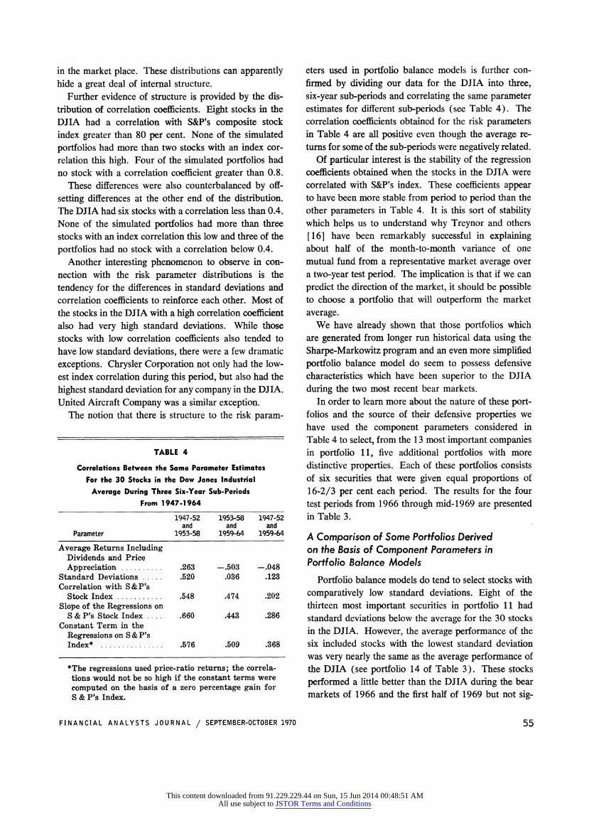
eters used in portfolio balance models is further con- firmed by dividing our data for the DJIA into, three, six-year sub-periods and correlating the same parameter estimates for different sub-periods (see Table 4). The correlation coefficients obtained for the risk parameters in Table 4 are all positive even though the average returns for some of the sub-periods were negatively related.

Of particular interest is the stability of the regression coefficients obtained when the stocks in the DJIA were correlated with S&P's index. These coefficients appear to have been more stable from period to period than the other parameters in Table 4. It is this sort of stability which helps us to understand why Treynor and others [ 16] have been remarkably successful in explaining about half of the month-to-month variance of one mutual fund from a representative market average over a two-year test period. The implication is that if we can predict the direction of the market, it should be possible to choose a portfolio that will outperform the market average.

We have already shown that those portfolios which are generated from longer run historical data using the Sharpe-Markowitz program and an even more simplified portfolio balance model do seem to possess defensive characteristics which have been superior to the DJIA during the two most recent bear markets.

In order to learn more about the nature of these portfolios and the source of their defensive properties we have used the component parameters considered in Table 4 to select, from the 13 most important companies in portfolio 11, five additional portfolios with more distinctive properties. Each of these portfolios consists of six securities that were given equal proportions of 16-2/3 per cent each period. The results for the four test periods from 1966 through mid-1969 are presented in Table 3.

A Comparison of Some Portfolios Derived on the Basis of Component Parameters in Portfolio Balance Models

Portfolio balance models do tend to select stocks with comparatively low standard deviations. Eight of the thirteen most important securities in portfolio 11 had standard deviations below the average for the 30 stocks in the DJIA. However, the average performance of the six included stocks with the lowest standard deviation was very nearly the same as the average performance of the DJIA (see portfolio 14 of Table 3). Thesie stocks performed a little better than the DJIA during the bear marke.ts of 1966 and the first half of 1969 but not sig-

TABLE 4

Correlations Between the Same Parameter Estimates For the 30 Stocks in the Dow Jones Industrial

Average During Three Six-Year Sub-Periods From 1947-1964

1947-52 1953-58 1947-52 and and and

Parameter 1953-58 1959-64 1959-64

Average Returns Including Dividends and Price Appreciation .......... .263 -.503 -.048

Standard Deviations ..... .520 .036 .123 Correlation with S&P's

Stock Index ........... .548 .474 .202 Slope of the Regressions on

S & P's Stock Index .660 .443 .286 Constant Term in the

Regressions on S & P's Index* ............... .576 .509 .368

*The regressions used price-ratio returns; the correlations would not be so high if the constant terms were computed on the basis of a zero percentage gain for S & P's Index.




nificantly better. It would appear that a defensive portfolio should not be chosen simply on the basis of those stocks with the least variance over some past period of time.-3

Portfolio 11 includes the six stocks in the DJIA with the lowest correlation with S&P's index. The average performance of these six securities was even more surprising than the performance of the six stocks with the lowest standard deviations. This portfolio, number 15, is clearly the least efficient portfolio in Table 3. It performed less well than the, DJIA during the two bear market years and much better than the DJIA during the bull market of 1967.

Most of the differential performance can be attributed to Chrysler Corporation, Westinghouse Electric and Swift. The prices of these three companies were poorly correlated with S&P's index from 1947-65 but have since been highly correlated with fluctuations in the market average. In the first two instances it would have been quite reasonable to have expected a much higher index correlation in subsequent periods since similar type companies such as General Motors and General Electric had much higher index correlations than Chrysler and Westinghouse. In the final analysis, the low correlations for these two companies may have been largely the result of temporary adversities that are infrequent and largely random in character.

One way to adjust the correlation coefficients for disturbances that are presumably random might be to sort firms on the basis of different industries and then regress the observed correlation coefficients on some indicator of intrinsic risk such as market share or aggregate sales. The calculated correlation coefficients could then be substituted for the actual coefficients to obtain a normal- ized risk parameter that is less influenced by historical accidents that are peculiar to individual firms.4 Accord- ing to the physicist P. W. Bridgman:

"In most laboratory situations repetition is not as a matter of fact the most effective way of dealing with the possibility of error. We are more likely to vary the conditions deliberately by small amounts for our successive measurements, and obtain in this way a succession of readings which we can plot. We then draw a smooth curve through the plotted points and expect that the curve will have a greater accuracy than the individual readings". [ 1, p. 174]

The tendency for stocks with relatively low correlation coefficients to "regress" to higher levels in subsequent

periods is of some importance in choosing a portfolio balance model. One reason our simplified portfolio balance model did not perform as well as the Sharpe- Markowitz program in the more recent bear markets is that relatively greater weight was given to stocks with comparatively low correlations. This does not seem to be a theoretical weakness of the model since the more exact Markowitz model has also been known to give greater weight to stocks with low correlations [9, Table 1, p. 1331, but could be of considerable practical importance if no attempt is made to adjust the historical correlations for accidental disturbances unrelated to a stock's normal propensity to fluctuate with the market.

Our next portfolio, number 16, gives equal weight to the six stocks in portfolio 11 with the highest average returns in the period from 1947-65. This particular portfolio consisted of United Aircraft which also had the highest average return for any stock in the DJIA, Eastman Kodak which ranked fourth (behind General Motors and Goodyear, excluded from portfolio 11 be- cause of their high correlation with S&P's index), Texaco, Chrysler, Standard Oil of New Jersey and Sears & Roebuck. The latter two companies ranked ninth and tenth in the DJIA (after Bethlehem Steel and U. S. Steel, excluded on the basis of both a high index correlation and a high standard deviation).

This portfolio is of particular interest since it appears to have outperformed the DJIA in both the bear markets of 1966 and 1969 and the major bull market of 1967. It was not quite as defensive as portfolios 11 and 12 but did have a higher average return over the four periods as a whole. Many investors would probably he happy to sacrifice some efficiency during bear markets in the hope of obtaining better than average performance over longer periods of time. This sort of trade-off is espe- cially apt to be important if the investor is not very successful in predicting the direction of the market.

When the individual stocks in the DJIA are regressed on S&P's composite index we obtain regression coefficients which figure prominently in the Sharpe-Markowitz portfolio model. This model tends to discriminate against companies with high slope coefficients. None of the ten stocks in the DJIA with the highest slope coefficients appeared in either the Sharpe-Markowitz portfolio or our more simplified portfolio balance model. Portfolio 17 consists of the six stocks in portfolio 11 with the highest slope coefficients. This portfolio behaved in an unpredictable fashion. It failed to outperform the DJIA during the bull market of 1967-when one would have expected better than average performance- and for the




four periods as a whole performed slightly less well, on the average, than the DJIA.

If a person was given a choice of component parameters to help him predict the ten stocks which appeared in both portfolios 11 and 12, he would have been wise to have selected the constant terms obtained when the percentage returns for individual securities are regressed on the percentage returns for S&P's composite index. All of the ten stocks in the DJIA with the highest constant terms were included in portfolios 11 and 12.

The six stocks ranked in order of the highest constant terms were United Aircraft, Eastman Kodak, Chrysler, General Foods, Westinghouse Electric, and Procter & Gamble. Portfolio 18 describes the average returns that could have been obtained by investing equal amounts of money in each of these six stocks during our four test periods from 1966-69. Since the constant terms were the best single predictor of the stocks included in portfolios 11 and 12, it is not too surprising that this portfolio turned out to be almost as defensive, on the average, as the more sophisticated portfolios.

The very high return for the bull market of 1967 is almost ten percentage points greater than was to be expected on the basis of the regression equations obtained during the original fitting period from 1947-65. This return was largely the result of Chrysler and Westing- house which were both poorly correlated with S&P's index in the original fitting period but have since fluctu- ated much more widely than the market average. Since both of the;se stocks declined more than the DJIA during the bear markets of 1966 and 1969 it is really quite re- markable that portfolio 18 turned out to be so defensive.

Portfolio 18 had an arithmetic average rate or price appreciation about 4.3 percentage points better than the average return from buying and holding the DJIA during our four test periods. This was more than one percentage point better than any of the other portfolios in Table 3. The higher average return was not entirely the result of Chrysler and Westinghouse. The average appreciation of these two stocks over the entire test period from the end of 1966 to mid-1969 was almost exactly the same as the average appreciation of the other four securities in portfolio 18. About 0.8 percentage points of the average difference between portfolio 18 and the DJIA can be attributed to the equalizing adjustments implicit in portfolio balance models; the remaining 3.5 percentage points are the result of having selected stocks which were relatively more resistant, on the average, to the general decline in stock prices which has occurred since the end of 1965.

While three and a half years is not a long enougb period to provide a very conclusive test of any forecasting system, it does seem clear that there is structure to some of the parameters used in portfolio balance models and that these models may be of assistance in selecting stocks that will be more defensive than the market average during periods of financial crisis. Such portfolios ought to be of interest to investors that are either risk averse or somewhat apprehensive about the future direction of stock prices.

If bull markets can be predicted with some degree of confidence, an investor may wish to consider portfolios somewhat less defensive than 1 and 12. We have ex- amined three different strategies for trying to beat the market in 1967 and 1968. The first strategy was to buy those six stocks which appreciated the most in the preceding year. This strategy has figured prominently in recent discussions of the random walk hypothesis [ 1i01]. During the period 1955-66 it would have worked rather well. The average return for the stars of the previous year was about five per cent greater, on the average, during this period than the average return for the 30 stocks in the DJIA.

The method did not work very well from 1947-54, however, nor has it worked very well in the last three years. The average price appreciation for those six stocks with the best preceding year performance was 8.7 per cent for 1967 and 1968 compared to 9.8 per cent for the DJIA.

Our second strategy was to invest equal amounts of money in those six stocks with the highest average returns for the entire DJIA in the period 1947-65. The average performance of these six stocks in 1967-68 was 12.5 per cent-about 2.5 per cent better than the DJIA.

Our third strategy was to invest equal amounts of money in those six stocks with the highest slope coefficients in the period 1947-65. If we accept the definition of risk proposed by Jensen [4] in his recent study of mutual fund performance, these six stocks-U. S. Steel, Bethlehem Steel, Anaconda, Goodyear, Alcoa, and In- ternational Paper -can be considered the six riskiest stocks in the DJIA. None of these six stocks were included in either portfolio 11 or 12. Their average appreciation in 1967-68 was 12.2 per cent-almost 21/2 percentage points better, on the average, than the DJIA.5

Suppose that a large fraction of the investing public believes it can forecast the general direction of the market with some degree of confidence. The optimal strategy, from a wealth maximizing point of view, would be to move out of defensive securities into more risky




investments when the market is bullish and to shift from risky issues to cash and more defensive securities when the outlook appears bearish. This sort of arbitrage would tend to reinforce the parameter structure which was observed for the DJIA.

With regard to whether the direction of the market can be forecast with some degree of confidence, it is our belief that investors who are attracted to the random walk hypothesis should at least keep an open mind. It is quite clear that the annual returns from holding common stock have been related in a fairly systematic way to both the business cycle [8] and to fluctuations in the money supply.6 [ 141 While changes in the latter two variables are sometimes difficult to forecast, we do not believe any economist would seriously contend that changes in the economy and the money supply are com- pletely random. *

APPENDIX A

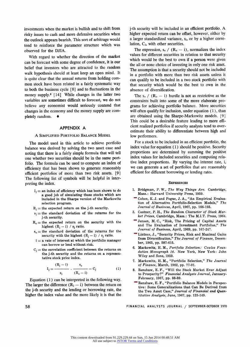
A SIMPLIFIED PORTFOLIO BALANCE MODEL

The model used in this article to achieve portfolio balance was derived by solving the two asset case and noting that there is a fairly simple formula that will teli one whether two securities should be in the same portfolio. The formula can be used to compute an index of efficiency that has been shown to! generate reasonably efficient portfolios of more than two risk assets. [9] The following list of symbols will be helpful in inter- preting the index.

Ij = an index of efficiency which has been shown to do a good job of simulating those stocks which are included in the Sharpe version of the Markowitz selection program.

Rj = the expected return on the j-th security.

sj = the standard deviation of the returns for the j-th security.

Ro = the expected return on the security with the highest (Ri - i) / sj ratio.

so = the standard deviation of the returns for the security with the highest (R3 - i) / sj ratio.

i = a rate of interest at which the portfolio manager can borrow or lend without risk.

Cj = the correlation coefficient between the returns on the j-th security and the returns on a representative stock price index.

(Ri-i) so Ij = . -j c(1)

sj (Ro-i)

Equation (1) can be interpreted in the following way. The larger the difference (Rj - i) between the return on the j-th security and the lending or borrowing rate, the higher the index value and the more likely it is that the

j-th security will be included in an efficient portfolio. A higher expected return can be offset, however, either by a larger standardized variance, sj, or by a higher correlation, Cj, with other securities.

The expression, so / (R. - i), normalizes the index values for different securities in relation to that security which would be the best to own if a person were given the all or none choice of investing in only one risk asset. The assumption is that a security should not be included in a portfolio with more than two risk assets unless it can qualify to be included in a two stock portfolio with that security which would be the best to own in the absence of diversification.

The so / (R. - i) hurdle is not as restrictive as the constraints built into some of the more elaborate programs for achieving portfolio balance. More securities will often qualify for inclusion, under equation (1), than are obtained using the Sharpe-Markowitz models. [9] This could be a desirable feature leading to more efficient realized portfolios if security analysts tend to over- estimate their ability to differentiate between high and low performers.

For a stock to be included in an efficient portfolio, the index value for equation ( 1 ) should be positive. Security proportions are determined by summing the positive index values for included securities and computing relative index proportions. By varying the interest rate, i, we can generate a set of portfolios that are reasonably efficient for different borrowing or lending rates.

REFERENCES

1. Bridgman, P. W., The Way Things Are. Cambridge, Mass.: Harvard University Press, 1959.

2. Cohen, K. J. and Pogue, J. A., "An Empirical Evalua- tion of Alternative Portfolio-Selection Models," The Journal of Business, April, 1967, pp. 166-193.

3. Cootner, P. H., The Random Character of Stock Mar- ket Prices, Cambridge, Mass.: The M.I.T. Press, 1964.

4. Jensen, M. C., "Risk, The Pricing of Capital Assets and The Evaluation of Investment Portfolios," The Journal of Business, April, 1969, pp. 167-247.

5. Lintner, J., "Security Prices, Risk and Maximal Gains from Diversification," The Journal of Finance, Decem- ber, 1965, pp. 587-615.

6. Markowitz, H. M., Portfolio Selection: Cowles Foun- dation Monograph 16. New York, New York: John Wiley and Sons, 1959.

7. Markowitz, H. M., "Portfolio Selection," The Journal of Finance, March, 1962, pp. 77-91.

8. Renshaw, E. F., "Will the Stock Market Ever Adjust to Prosperity?" Financial Analysts Journal, January- February, 1967, pp. 88-89.

9. Renshaw, E. F., "Portfolio Balance Models in Perspec- tive: Some Generalizations that Can Be Derived from the Two Asset Case," Journal of Financial and Quan- titative Analysis, June, 1967, pp. 123-149.




10. Renshaw, E. F., "The Random Walk Hypothesis, Per- formance Management, and Portfolio Theory," Finan- cial Analysts Journal, March-April, 1968, pp. 114-118.

11. Sharpe, W. F., "A Simplified Model for Portfolio Analysis," Management Science, January, 1963, pp. 277-293.

12. Smith, K., "Alternative Procedures for Revising In- vestment Portfolios," Journal of Financial and Quan- titative Analysis, December, 1968.

13. Smith, K. V., "A Transition Model for Portfolio Re- vision," The Journal of Finance, September, 1967.

14. Sprinkel, B. W., Money and Stock Prices. Homewood, Illinois: Richard D. Irwin, 1964.

15. Tobin, J., "Liquidity Preference as Behavior Towards Risk," Review of Economic Studies, February, 1958, pp. 65-86.

16. Treynor, J. L., Priest, W. W., Fisher, L., and Higgins, C. A., "Using Portfolio Composition to Estimate Risk," Financial Analysts Journal, September-October, 1968, pp. 93-102.

FOOTNOTES

1. This figure is for the 12-year period from 1952-64. 2. See Tobin's expansion of Markowitz's efficient set [15]. 3. Three stocks with comparatively low standard devia-

tions, AT & T, Union Carbide, and Allied Chemical did

not enter significantly into portfolio 11. When these stocks are included in the six stocks with the lowest standard deviation for the entire DJIA we obtain a value of .908 for the first six months of 1969, compared to a value of .925 for the DJIA and a value of .780 for 1966 compared to .811 for the DJIA.

4. Another possibility that ought to be considered in this context is to regress the correlation coefficients for different firms on their associated standard deviations. These two parameters tended to be positively related in both the DJIA and our simulated portfolios.

5. The surprising thing about this portfolio is that most of the advantage over the DJIA occurred in 1968, which was not a bullish year for the majority of stocks in the DJIA.

6. About ten per cent of the variation in annual returns including dividends associated with S&P's composite stock index can be explained by corresponding changes in the money supply from 1924-52. In the more recent period from 1953-65 this percentage jumps to over 35 per cent; when a trend term is included in the regression, the square of the correlation coefficient rises to nearly 65 per cent. When the latter equation was used to explain subsequent behavior we obtained an implied loss of 7.1 per cent for 1966 which was very nearly equal to the 9.7 per cent loss which actually occurred in that year.

Characteristics of Sales Forecasts... CONTINUED FROM PAGE 46

is documented in Table 5. It means that, if other things are equal, the forecaster is likeliest to do well in those cases where it matters most.6

Collaboration With the Industry Specialists

The working partnership of industry specialist and statistician-forecaster seems to be one of those happy wholes which is much greater than the sum of its parts. Each member of the team finds his own task transform- ed in many respects by the other's contribution.

An example from the statistician's point of view was noted at the beginning of this article. In contrast to the usual rule, such a team can make better use of a formula that mostly gives excellent results but occasionally goes far astray than they can of a consistently mediocre formula.

The advantages of the collaboration do not come about automatically, however. They have to be worked for. BDSA's econometric forecasting unit has found cer- tain practices helpful in this connection. We try to avoid symbols and abbreviations in our presentation to the industry specialists. We make a systematic attempt to suit our standard format to their characteristic ways of thinking about their industry. Above all, we try to be

as specific as possible about the way the projection might actually come to pass: the respective contributions of price and volume increases, for example; and the contributions of different segments of the industry's markets. We then urge the specialists, when they modify our initial formula projections, to do so in terms of these factors. Another experiment now in progress will illustrate these efforts, and is of some interest in its own right beside.

Forecasts in Market-Sector Detail

If one had any information or impressions at all sug- gesting that some customer groups might fare better than others in the year ahead, ideally one would prefer to study the various customer categories separately. BDSA has attempted to project market detail for some of the broad industry groups distinguished in the 1958 input-output table. We estimated the relative importance of different customers by use of multiple regression techniques, and checked the results against what would have been expected in the light of the 1958 pattern of inter-industry transactions.

Of course the latter would be somewhat different in any case. The year 1958 was not very typical of the




Documents

Simulating the Dow Jones Industrial Average: A Further Test of the Random Walk Hypothesis