SIMULATION METHOD FOR PARTICLE

ADHESION IN VEHICLE COOLING SYSTEMS

FINAL REPORT

Prepared by

Jeffrey S. Marshall, John Mousel and Shuiqing Li

Submitted to

Caterpillar Technical Center Youssef M. Dakhoul, Project Manager

IIHR Technical Report # 459

IIHR − Hydroscience & Engineering College of Engineering The University of Iowa

Iowa City, IA 52242-1585 USA

December 2006

i

Summary

An efficient computational method was developed for transport, collision and aggregation of small adhesive particles. A level-set method was used on a background Cartesian grid to rapidly advect particles in complex geometrical domains. The method has been developed with both van der Waals and liquid-bridging adhesion forces. The computational method was tested for a variety of two- and three-dimensional problems. In two dimensions, the method is used to examine particle capture by walls in periodic channel flows and in nozzles with various contraction lengths. For channel flow, it is found that particle capture by the channel walls is dominated by collisions of free-floating aggregates with aggregates attached to the wall. This collision can result in capture of the aggregate by the wall-attached aggregate or tearing of the wall-attached aggregate and re-entrainment into the flow. Particle adhesion in nozzle flow is shown to result in formation of aggregates both due to the stretching of fluid elements as they pass through the nozzle and from development of aggregates on the nozzle wall and resuspension back into the flow. Similar aggregate collision and adhesion processes are observed to control particle wall capture in three-dimensional periodic pipe flow. For the problem of particle capture by a cylindrical fiber array, the particles are observed to collect on the front face of the fiber. Comparison of the length of the collected particles is found to compare well with experimental data. Preliminary computations are then used for flow of a dusty fluid through a section of a radiator, consisting of a vertical support and neighboring cooling channels. The flow field through the radiator section is computed using U2RANS, a finite-volume general-use fluid flow code developed at IIHR – Hydroscience and Engineering. Particles are advected through the radiator section and shown to adhere to the front side of the vertical support, as well as adhesion to a lesser extent to the particle channel walls. The computational method is found to be highly efficient and accurate for computation of particle wall capture in dusty fluid flows in complex geometrical domains, including a section of a radiator flow. The second phase of the research will use this code to examine strategies for mitigation of particle build-up on radiators, including steady and unsteady fluid flow with various orientations, in both the forward and backward directions, and electromagnetic pulsing. The results of these computations will be validated experimentally using the Caterpillar dusty wind tunnel facility.

ii

iii

Simulation Method for Particle Adhesion in Vehicle Cooling Systems

TABLE OF CONTENTS

Contents Page I. Introduction and Objectives.................................................................................... 1 II. Simulation Method.................................................................................................. 1

A. Fluid forces and torques .................................................................................... 2 B. Collision forces and torques............................................................................... 3 C. Van der Waals adhesion .................................................................................. 12 D. Liquid bridging adhesion ................................................................................. 14 E. Level set method for simulation with complex geometries ............................. 16

III. Two-Dimensional Test Cases… ........................................................................... 22

A. Channel flow ................................................................................................... 22 B. Nozzle flow ..................................................................................................... 30

IV. Three-Dimensional Test Cases ............................................................................ 37

A. Pipe flow ......................................................................................................... 37 B. Fiber filter array ............................................................................................... 43

V. Radiator Flows ..................................................................................................... 50

A. Grid and velocity field .................................................................................... 50 B. Preliminary results for particle adhesion ......................................................... 51

VII . References Cited ................................................................................................ 53 VIII. List of Staff Working on Project........................................................................ 57 IX. List of Papers and Theses .................................................................................... 57

A. Journal articles ................................................................................................ 57 B. Thesis .............................................................................................................. 58 C. Conferences ..................................................................................................... 58

iv

1

Simulation Method for Particle Adhesion in Vehicle Cooling Systems I. Introduction and Objectives Caterpillar vehicles operate in environments filled with particulate matter of various types, including sand and dirt particles, mine dust, and metal shavings. These particles vary greatly in size and density. Under certain conditions, particles can clog vehicle radiators after relatively short operation times. While large particles can be removed from the inlet air stream by screens or centrifugal pre-cleaners, it is often the small particles (10-100 µm diameter) that are most problematic in clogging cooling channels. These particles adhere to radiator surfaces through a variety of forces, including van der Waals, liquid bridging, and electrostatic and magnetic forces, under different environmental conditions. Numerical prediction of particle adhesion requires the ability of a CFD code to account for both particle collisions and a wide range of adhesion forces. This can be a challenge due to the fact that most adhesion forces act over distances of a nanometer or less, which is much smaller than the particle diameter. Commercial CFD codes do not offer any capabilities for modeling particle adhesion. At the same time, empirical tests are expensive and difficult to conduct over the wide range of particle types, moisture levels, and operating conditions that are known to lead to particle clogging problems. The current project is Phase I of what is proposed to be a two-part effort. Phase I examined the feasibility of developing an efficient computational model for simulation of particle adhesion in vehicle cooling systems. The proposed particle transport code is developed as a stand-alone code which can be coupled to a variety of fluid flow codes. In our current work, we utilize the particle code in conjunction with to an existing fluid flow simulation code (U2RANS) developed at IIHR-Hydroscience and Engineering. The particle transport code developed in the current project was tested for a series of simplified geometries characteristic of different regions of the radiator flow field. Preliminary computations were performed for particle transport and adhesion in the radiator flow domain, consisting of a series of radiator channels on either side of a section of a support bar. The second part (Phase II) of the project will utilize this code to develop and test mitigation strategies for removal of dust particle build-up on construction vehicle radiators. II. Simulation Method We seek to develop a fast, accurate computational method for simulation of dust particle adhesion in flow fields with complex geometry, in particular a vehicle radiator. We further seek to utilize these methods to understand the physical mechanisms leading to cooling system clogging under different environmental situations, which includes different humidity conditions and different particle types. We ultimately seek to utilize this knowledge to develop mitigation strategies to dramatically reduce cooling system clogging problems.

2

The discrete-element method solves for the velocity v and rotation rate Ω of each particle by solution of the linear and angular momentum equations

AFdtdm FFv += , AFdt

dI MMΩ += (1)

where m is the particle mass, d is the particle diameter, 2)10/1( mdI = is the particle momentum of inertia, and dtd / is the derivative following a moving particle. The forces acting on the particle are the fluid force ( FF ) and the collision and van der Waals adhesion forces, which are together denoted as AF . In the angular momentum equation,

FM and AM denote the corresponding fluid torque and the sum of the collision and van der Waals adhesion torques on the particle. Use of a soft-sphere DEM for colliding particles entails resolution of the particle collision process, which requires very small time steps for solution accuracy. The presence of adhesive forces further reduces the required time step, since small variations of the particle separation distance within the region of closest contact must be finely resolved. In order to adequately resolve the particle motion at these widely diverse time scales, Marshall (2006a) proposed an algorithm using three different time steps – the fluid time step ULft /1=∆ on which the fluid flow is updated, the particle time step UdftP /2=∆ use to evolve particles that are not involved in a collision, and the collision time step

5/1223 )/( UEdft ppC ρ=∆ used to evolve particles that are involved in a collisions. Here

1f , 2f , and 3f are all small parameters, and the time scales are ordered such that CP ttt ∆>>∆>>∆ . In these equations, L and U are characteristic length and velocity

scales of the fluid flow, and pρ and pE are the particle density and Young’s modulus. To accelerate the computation, a list of nearby particles is stored for each particle, which is recomputed every fluid time step. This “local-list” is constructed by sorting the particle onto a Cartesian grid, whose grid increment is set equal to the “search radius” of the particle, and then searching through the grid cell in which a particle resides and all neighboring grid cells. We identify colliding particles at each particle time step, where the collision and adhesion forces of the colliding particles are recomputed each collision time step. As a typical example, we consider dust particles in a radiator flow in air. For dust particle diameter of m 10 µ and fluid length and velocity scales of mm1=L and cm/s1=U , respectively, the fluid-to-particle density ratio is 4106.4/ −×≅≡ pf ρρχ , the dimensionless particle diameter is 01.0/ =≡ Ldε , and the corresponding Stokes number is 01.0)18/(Re18 22 ≅=≡ χεµρ Fp LUdSt . Setting 132 10 fff == , the ratio of the fluid time scale to the particle time scale is 10/ =∆∆ Ptt . Using a particle elastic modulus of GPa 5≅pE , the ratio of the particle time scale to the collision time scale is

270,12/ ≅∆∆ CP tt , resulting in 120,000 collision time steps per fluid time step. Even

3

with the multiple time-step algorithm, it is usually necessary to assume a much lower elastic modulus for the dust particles in order to make the computations feasible. A. Fluid Forces and Torques Fluid forces on the particles include drag, lift, pressure gradient (or buoyancy), gravity, added mass force, and Magnus force. The particle Reynolds number, ν/Re dP uv −≡ where u is the fluid velocity at the particle location and fρµν /= is the fluid kinematic viscosity, and the dimensionless particle diameter Ld /≡ε are both assumed to be much smaller than unity. For small particles, the dominant fluid force is usually the drag force dF , given by fdd )(3 uvF −−= µπ . (2) The Stokes drag solution for an isolated sphere is recovered for friction factor 1=f . We use the correlation of Di Felice (1994) to correct friction factor to account for particle crowding in non-dilute flows, giving β−−= )1( cf , (3) where ),( tc x is the local particle concentration (i.e., the ratio of the particle volume to the fluid volume in a small region around the particle) and β is given by

⎟⎠⎞

⎜⎝⎛ −−−= 2)]ln(Re5.1[

21exp65.07.3 Pβ . (4)

The reduced gravity force gF is gF )1( χ−= mg , (5) where g is the gravitational acceleration vector. The pressure gradient force pF , due to the acceleration of the external flow past the particle, is

DtDmp

uF χ= , (6)

where DtD / denotes the rate of change with time following a fluid particle, such that

uuvuu ])[( ∇⋅−−=dtd

DtD . (7)

4

The added mass force aF is given by

)(dtd

dtdmcMa

uvF −−= χ , (8)

where the added mass coefficient for a sphere is 2/1=Mc . The ratio

)(/)or ( χOFFF dap ≈ , so these forces are generally small when the particle density is much greater than the fluid density. A particle placed in a shear flow exhibits a lift force lF in the direction normal to the direction of the flow. If the particle is assumed to rotate at the same rate as the local rotation rate of fluid particles, the lift force solution of Saffman (1965, 1968) can be written as

2/12/1Re)(18.2

LP

mα

χ ωuvF ×−−=l , (9)

where )2/( uvω −≡ dLα . The ratio )(/ 2/1SOFF d ε=l , where νω /2LS ≡ is a dimensionless shear parameter. For small particles ( 1<<ε ), the lift force is generally small compared to drag except in regions of very large vorticity. We note that the Basset history force bF is neglected in this model since for small particles the ratio of Basset force to drag scales as 1Re/ 2/1 <<≅ pdb FF . A detailed discussion of the effects of Basset force on particle motion is given by Druzhinin and Ostrovsky (1994). When the particle rotation rate differs from that of the surrounding fluid, an additional “Magnus” force mF is exerted on the particles, given by

)()21(

43 uvΩωF −×−−= mm χ . (10)

The ratio )(/ SOFF dm ε= , so Magnus force tends to be important under the same conditions that particle lift is important. The corresponding torque on the particle due to local fluid rotation is given by

)21(3 ΩωM −= dF πµ . (11)

In additional to the forces listed above, it often necessary to include a random force acting on the particles. For very small particles (less than a micron diameter), this random force results from the Brownian motion induced by individual molecular collisions with

5

the particle. For turbulent flows, a random force is often used to model effects of subgrid-scale turbulence on dispersion of the particles. A review of random force models for particulate flows is given by Crowe et al. (1998). The particles exert a body force on the fluid flow. This body force is computed by determining the fluid grid cell in which each particle lies and distributing the force

ngF )( FF −− on the fluid imposed by particle n onto the surrounding grid nodal points by the equation

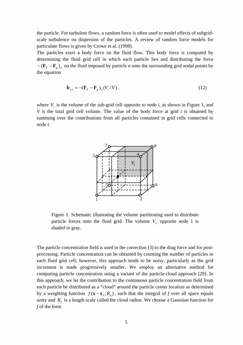
)/()(, VVingFin FFb −−= . (12)

where iV is the volume of the sub-grid cell opposite to node i, as shown in Figure 1, and V is the total grid cell volume. The value of the body force at grid i is obtained by summing over the contributions from all particles contained in grid cells connected to node i.

1 2

3 4

5 6

7 8

V1

Figure 1. Schematic illustrating the volume partitioning used to distribute particle forces onto the fluid grid. The volume 1V opposite node 1 is shaded in gray.

The particle concentration field is used in the correction (3) to the drag force and for post-processing. Particle concentration can be obtained by counting the number of particles in each fluid grid cell; however, this approach tends to be noisy, particularly as the grid increment is made progressively smaller. We employ an alternative method for computing particle concentration using a variant of the particle-cloud approach [29]. In this approach, we let the contribution to the continuous particle concentration field from each particle be distributed as a “cloud” around the particle center location as determined by a weighting function ),( nn Rf xx − , such that the integral of f over all space equals unity and nR is a length scale called the cloud radius. We choose a Gaussian function for f of the form

6

]/exp[3

2),( 22

3 nnn

nn RR

Rf xxxx −−=−π

. (13)

The concentration ),( tc x at a point x is obtained by summing over the contributions of the nearby particle clouds as

),(),(1

nnn

N

nRfAtc xxx −=∑

=, (14)

where the cloud amplitude nA and cloud radius nR are held constant for each computational particle. The cloud amplitude is equal to the particle volume, or

3)6/( nn dA π= , such that the integral of the concentration field over all space equals the sum of all the particle amplitudes, or the total volume occupied by the particles. B. Collision Forces and Torques The forces and torques acting on the particles are decomposed into four parts: that acting along the line normal to the particles centers and the resistance from sliding, twisting, and rolling of one particle over another (Figure 2). The normal force acts in the direction of the unit vector n which points tangent to the line connecting the centers of the two particles, denoted by i and j, such that ijij xxxxn −−= /)( . Since for spherical particles the normal force acts in the direction n passing through the particle centroids, it exerts no torque on the particles. The sliding resistance acts in a direction St , corresponding to the direction of relative motion of the particle surfaces at the contact point projected onto the contact plane (the plane orthogonal to n). The sliding resistance also imposes a torque on the particle in the Stn× direction. The twisting resistance exerts a moment on the particle in the n direction, normal to the contact plane. The rolling resistance exerts a torque on the particle in the nt ×R direction, where Rt is the direction of the “rolling” velocity, which we define later in this section. The total collision and adhesion force and torque fields on particle i can then be written as

SsnA FF tnF += , nnttnM tRrSsiA MMFr +×+×= )()( , (15)

where ir is the radius of particle i.

7

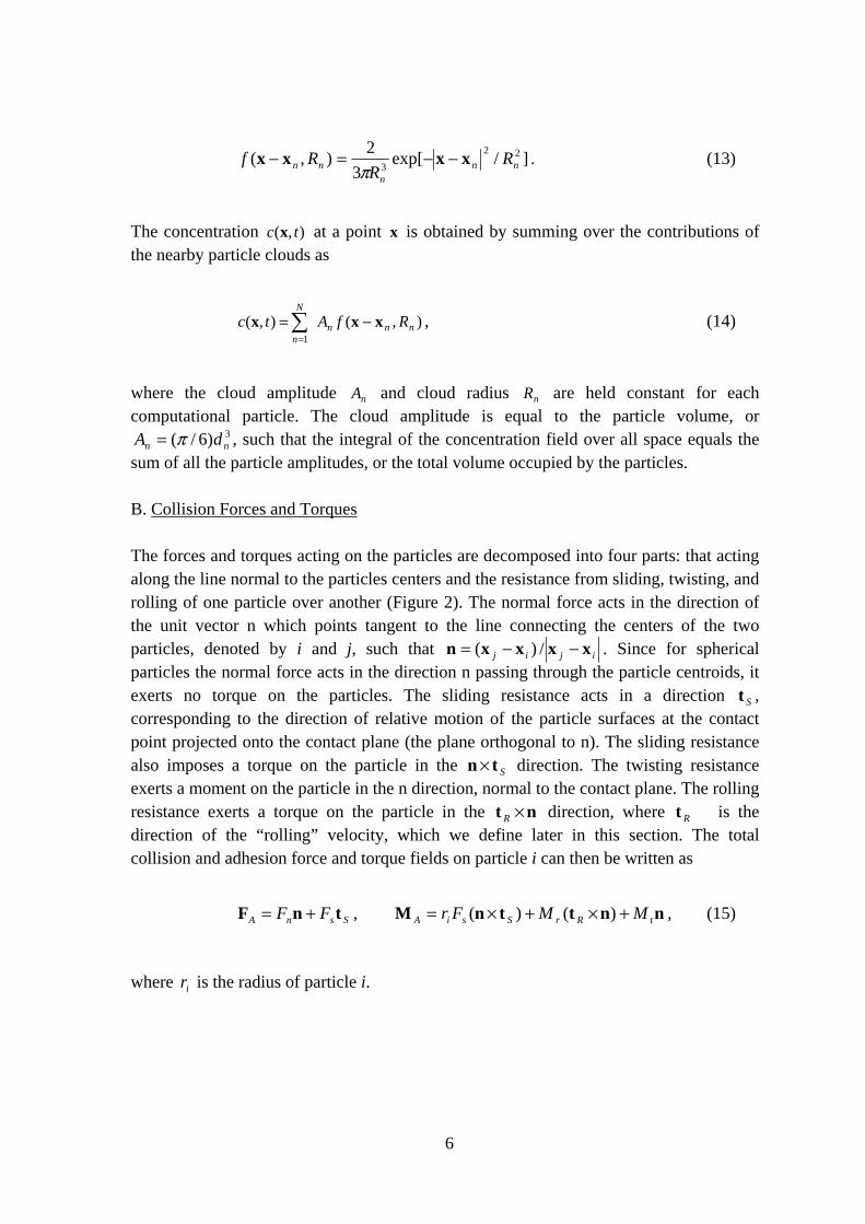
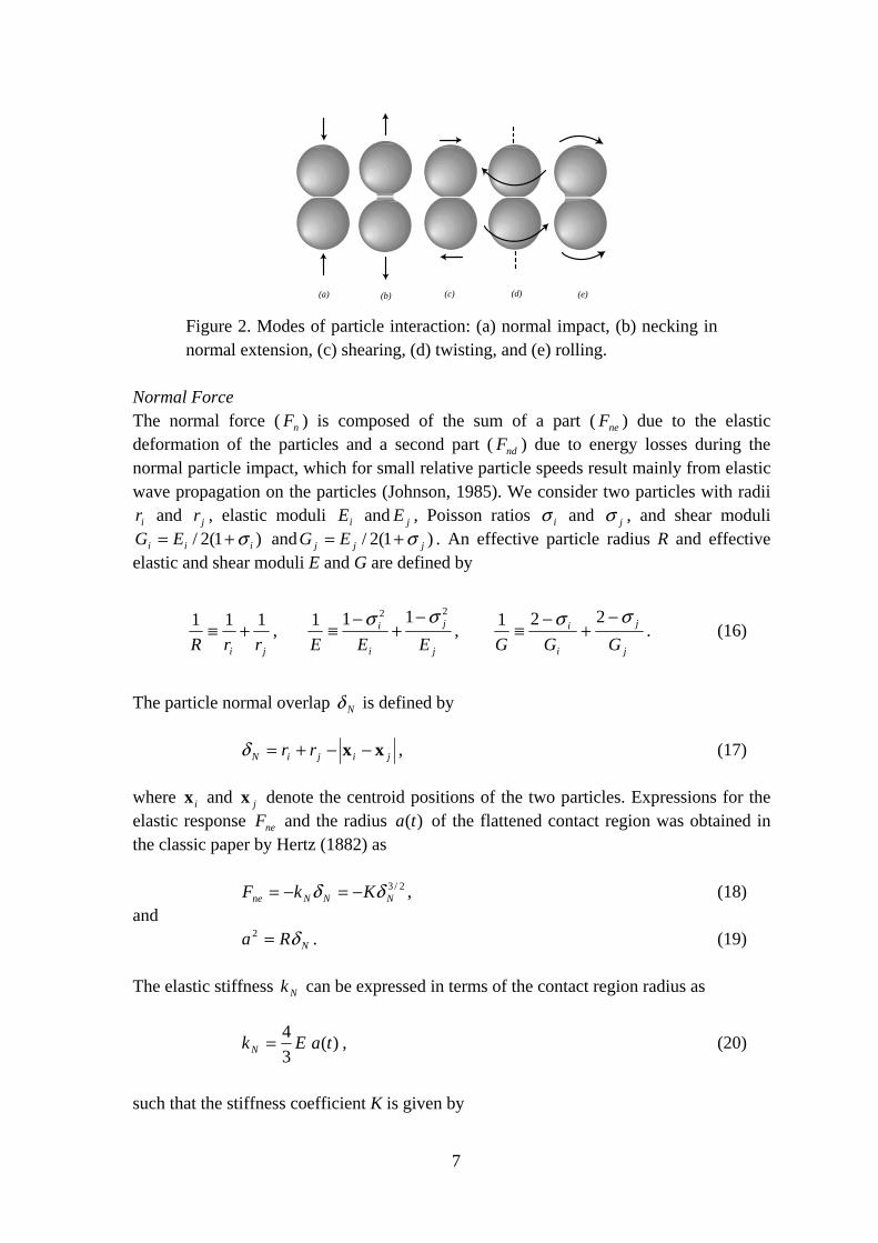
(a) (b) (c) (d) (e) Figure 2. Modes of particle interaction: (a) normal impact, (b) necking in normal extension, (c) shearing, (d) twisting, and (e) rolling.

Normal Force The normal force ( nF ) is composed of the sum of a part ( neF ) due to the elastic deformation of the particles and a second part ( ndF ) due to energy losses during the normal particle impact, which for small relative particle speeds result mainly from elastic wave propagation on the particles (Johnson, 1985). We consider two particles with radii

ir and jr , elastic moduli iE and jE , Poisson ratios iσ and jσ , and shear moduli )1(2/ iii EG σ+= and )1(2/ jjj EG σ+= . An effective particle radius R and effective

elastic and shear moduli E and G are defined by

ji rrR

111 +≡ , j

j

i

i

EEE

22 111 σσ −+

−≡ ,

j

j

i

i

GGGσσ −

+−

≡221 . (16)

The particle normal overlap Nδ is defined by jijiN rr xx −−+=δ , (17) where ix and jx denote the centroid positions of the two particles. Expressions for the elastic response neF and the radius )(ta of the flattened contact region was obtained in the classic paper by Hertz (1882) as 2/3

NNNne KkF δδ −=−= , (18) and NRa δ=2 . (19) The elastic stiffness Nk can be expressed in terms of the contact region radius as

)(34 taEkN = , (20)

such that the stiffness coefficient K is given by

8

REK34= . (21)

The dissipation force ndF is given by nv ⋅−= RNndF η , (22) where iiiiC rΩvv ×+=, is the surface velocity of particle i at the contact point, nr ii r= and nr jj r−= are the vectors from the particle centroids to the contact point,

CjCiR vvv −= is the relative particle surface velocity at the contact point, and Nη is the normal friction coefficient. Cundall and Strack (1979) and Tsuji et al. (1992) propose expressions for Nη in which 2/1)( NN mk∝η , where NneN Fk δ/= is the normal stiffness coefficient. Tsuji et al. (1992) propose that the damping coefficient is related to the coefficient of restitution if Nη is assumed to have the form 2/1)( NN mkαη = , (23) where α is a coefficient of friction that is written as a function of the restitution coefficient of the particles (see Section 7). Other expressions for Nη have also been proposed. For instance, Brilliantov et al (1996) examine the damping produced by collisions of two viscoelastic particles and propose an expression for normal damping coefficient where aN ∝η , whereas substitution of (20) into (23) gives 2/1aN ∝η . Since most of the literature on normal particle collision reports results in terms of the restitution coefficient, it is often convenient to use the expression (23) for Nη and then account for effects such as viscous fluid damping (Barnocky and Davis, 1989) and material viscoelastic or wave propagation losses through modification of the restitution coefficient. Sliding Resistance We adopt a spring-dashpot-slider model for the sliding resistance proposed by Cundall and Strack (1979). In this model, the tangential sliding force sF is first absorbed by the spring and dashpot until its magnitude reaches a critical value nfcrit FF µ= . The friction coefficient fµ has a typical value of about 0.3 for dry surfaces, but can be substantially reduced by the presence of the fluid within the contact region, particularly for smooth particle surfaces. If crits FF > , then the particle surfaces will slip and the friction coefficient will be given by the modified Amonton friction expression crits FF −= . (24) For the subcritical case crits FF < , the sliding resistance due to the spring and dashpot for particle i yields

9

SSTS

t

tSTs dkF tvtv ⋅−⋅−= ∫ ηττ ))((

0

, (25)

where the slip velocity )(tSv is the tangent projection of Rv to the particle surface at the contact point, or

nnvvv )( ⋅−= RRS (26)

and the slip direction is SSS vvt /= . The first term on the right-hand side of (25) is an elastic spring and the second term is viscous friction. The time integral in the first term gives the tangential elastic displacement of the material before slipping sets in, where 0t is the time of initial particle impact. An expression for the tangential stiffness coefficient Tk is derived by Mindlin (1949). Rewriting this expression in terms of the contact region radius )(ta gives )(8 taGkT = . (27) Tsuji et al. (1992) assume that the tangential dissipation coefficient is of the same order as the normal viscous damping coefficient, so that lacking further information they set

NT ηη = . Other investigators in granular flows omit the last term in (25), which reduces to the common stick-slip friction model. Twisting Resistance Twisting occurs when the two colliding particles have different rotation rate in the direction n (Figure 2d). The relative twisting rate TΩ is defined by nΩΩ ⋅−=Ω )( jiT , (28) In analogy to the friction model (25) used for sliding, we propose a twisting resistance expression of the form

TQT

t

tQt dkM Ω−Ω−= ∫ ηξξ )(

0

. (29)

Here the time integral represents the angular displacement prior to torsional sliding. The expression (29) can be derived from (25) by integrating the friction stress 2/ aFs π over the contact area with relative velocity RR rv Ω= oriented in the azimuthal direction, giving

10

TT

T

t

t

Ts

a

ta

dak

drrrFa

M Ω−Ω−== ∫∫ 2)(

2)(2 22

2

02

0

ηξξ . (30)

Comparing (29) and (30) yields the torsional stiffness and friction coefficients as 2/2akk TQ = , 2/2aTQ ηη = . (31) The particles will begin to spin relative to each other when the torque exceeds a critical value. The critical torque can be derived by integrating the moment 2/ arFcrit π due to the critical sliding stress over the contact region, yielding

critcritt aFM32

, = . (32)

When crittt MM ,> , the torsional resistance is given by TTcrittt MM ΩΩ−= /, . (33) Rolling Resistance Several computational and experimental studies have pointed out that rolling, rather than slipping or twisting, is the primary micro-deformational mechanism in granular flows and materials with small particle sizes (Bardet, 1994; Iwashita and Oda, 1998; Oda, 1982). Rolling is related to the change in position of the particle-particle contact point due to the particle rotation. The particles are simultaneously undergoing several different motions, including sliding, twist, and solid-body rotation of the particle aggregate, in addition to rolling, and there are several different ways that the rolling motion has been defined in the literature as distinct from these other motions. A discussion of four different definitions of rolling and of the effect of rolling motion on granular particle dynamics is given by Kuhn and Bagi (2004). An expression for the rolling displacement of arbitrary-shaped particles is derived by Bagi and Kuhn (2004) which is objective, such that the rolling velocity is independent of the reference frame in which it is measured. This property is important in part to ensure that the rolling motion is independent of solid-body rotation of the particle aggregate. Taking the rate of this expression and specializing to spherical particles yields an equation for the “rolling velocity” Lv of particle i as

Sij

ijjiL rr

rrR vnΩΩv )(

21)(

+−

−×−−= . (34)

11

The first term is the velocity due to the difference in rotation rate of the particles projected onto the plane orthogonal to n. The last term accounts for the effect of different particle size on rolling velocity. This definition reduces to that of Iwashita and Oda (1998) when applied to a circular disk. We define the direction of rolling as

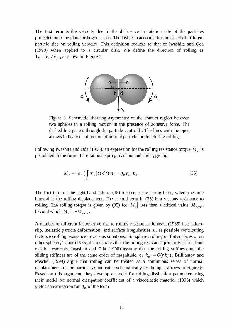
LLR vvt /= , as shown in Figure 3.

Ω i Ω j

n

Figure 3. Schematic showing asymmetry of the contact region between two spheres in a rolling motion in the presence of adhesive force. The dashed line passes through the particle centroids. The lines with the open arrows indicate the direction of normal particle motion during rolling.

Following Iwashita and Oda (1998), an expression for the rolling resistance torque rM is postulated in the form of a rotational spring, dashpot and slider, giving

RLRRL

t

tRr dkM tvtv ⋅−⋅−= ∫ ηττ ))((

0

. (35)

The first term on the right-hand side of (35) represents the spring force, where the time integral is the rolling displacement. The second term in (35) is a viscous resistance to rolling. The rolling torque is given by (35) for rM less than a critical value critrM , , beyond which critrr MM ,−= . A number of different factors give rise to rolling resistance. Johnson (1985) lists micro-slip, inelastic particle deformation, and surface irregularities all as possible contributing factors to rolling resistance in various situations. For spheres rolling on flat surfaces or on other spheres, Tabor (1955) demonstrates that the rolling resistance primarily arises from elastic hysteresis. Iwashita and Oda (1998) assume that the rolling stiffness and the sliding stiffness are of the same order of magnitude, or )(0 TiR krOk = . Brilliantov and Pöschel (1999) argue that rolling can be treated as a continuous series of normal displacements of the particle, as indicated schematically by the open arrows in Figure 5. Based on this argument, they develop a model for rolling dissipation parameter using their model for normal dissipation coefficient of a viscoelastic material (1996) which yields an expression for Rη of the form

12

neRR Fµη = , (36) The rolling coefficient Rµ is related to the coefficient of restitution e by

5/25/10 )/(

1mKwb

eR

−=µ , (37)

where the constant b is given by 283.2≅b and 0w is a measure of the relative normal velocity between the particles prior to collision. C. Van der Waals Adhesion Following the approach of Johnson et al. (1971), we assume that van der Waals adhesive force acts only within the flattened contact region. The separation of the particles is further assumed to remain constant within this contact region, due to the effect of the short-range van der Waals repulsive force, so that the adhesive force can be described using a surface potential γ, defined such that 22 aπγ is the work that must be performed to separate the surfaces if the particles are treated as rigid bodies. Normal Force For very slow particle impact velocities and with no fluid forces, the two particles approach an equilibrium state in which the elastic repulsion is balanced by the adhesive attraction of the particles. In this equilibrium state, the radius )(ta of the contact region is given by

3/12

09

⎟⎟⎠

⎞⎜⎜⎝

⎛=

ERa πγ . (38)

The expressions (18)-(19) for contact region radius and elastic rebound force neF are modified in the presence of van der Waals force, and can be written as (Chokshi et al., 1993)

2/3

0

3

0

44 ⎟⎟⎠

⎞⎜⎜⎝

⎛−⎟⎟

⎠

⎞⎜⎜⎝

⎛=

aa

aa

FF

C

ne (39)

and

⎥⎥⎦

⎤

⎢⎢⎣

⎡⎟⎟⎠

⎞⎜⎜⎝

⎛−⎟⎟

⎠

⎞⎜⎜⎝

⎛=

2/1

0

2

0

3/1

3426

aa

aa

C

N

δδ

. (40)

13

In these equations, the critical force and overlap, CF and Cδ , are given by

RFC πγ3= , R

aC 3/1

20

)6(2=δ . (41)

The force neF is defined to be positive when it pushes the two particles toward each other. As the two particles move away from each other due to an applied stretching from the fluid or the particle inertial force, contact will be maintained even for negative values of Nδ via necking of the particle material (Figure 2b), until the critical point is reached, at which Cne FF −= and CN δδ −= . As the particles are pulled further apart, the contact will suddenly break. To minimize the computational time, we pre-compute Cne FF / and

0/ aa as functions of CN δδ / at the beginning of the calculation, and then use a look-up table to determine neF and )(ta for the given value of Nδ at each time step. By writing

Nk in terms of the contact region radius a in (20), rather than the more traditional form in terms of the overlap Nδ , we can use the same expressions (22)-(23) for the normal dissipation force as used for cases with no adhesion. Sliding and Twisting Resistance The effect of van der Waals adhesion on tangential sliding force was examined by Savkoor and Briggs (1977), and a simplified model was proposed by Thornton (1991) and Thornton and Yin (1991). Sliding is relatively rare for adhesive particles due to their small momentum, and it is of importance mainly in cases where an aggregate is torn apart by a fluid shear of by adhesion to another aggregate. To save computational time, we therefore adopt a simplified sliding resistance model proposed by Thorton (1991), which was found to agree reasonably well with experimental data. This simplified approach uses the same expressions (24)-(27) that were developed for the case with no adhesive force, but replaces the critical sliding force by Cnefcrit FFF 2+= µ , (42) where CF is given in (41). The addition of the CF2 term in (42) is necessary to ensure that the critical tangential force approaches Cf Fµ at the critical point when the particles are just about to separate. Similarly, the twisting resistance has the same form described in Section 4, but with the critical torque replaced by

CNfcritt FFaM 232

, += µ . (43)

Rolling Resistance The van der Waals adhesion force leads to an additional mechanism for rolling resistance by inducing an asymmetry in the contact region, as shown in Figure 3, due to the pulling apart of the particles surfaces on one side of the contact point and the pushing together of

14

the particle surfaces on the other side. An expression for the torque induced by this adhesion-induced asymmetry is derived by Dominik and Tielens (1995) as ξ2/3

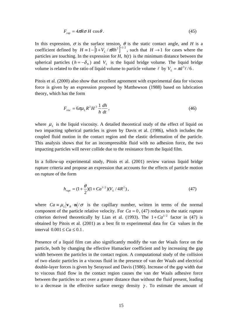
0 )/(4 aaFM Cr −= , (44) where ξ is the displacement of the particle centroid due to rolling in the Rt direction, given by the time integral in (30). Dominik and Tielens (1995) further argue that the critical resistance occurs when the rolling displacement ξ achieves a critical value, corresponding to a critical rolling angle Rcritcrit /ξθ = . For critξξ > , the rolling displacement ξ in (44) is replaced by critξ . D. Liquid Bridging Adhesion In a humid environment, each aerosol particle is surrounded by a film of liquid. When two particles collide, their liquid films will join to form a “liquid bridge” stretching between them (Figure 4). This liquid bridge introduces a capillary force capF that pulls the two particles toward each other, leading to adhesion of the particles. In addition, the liquid film introduces an enhanced frictional force viscF between the particles due to the higher viscosity of the liquid compared to that of the surrounding gas. The total liquid bridge force is given by the sum nF )( visccapL FF += . Computation of particle collision with liquid bridging adhesion requires models for both the capillary and viscous forces on the particles, as well as a criterion for rupture of the liquid bridge at a critical separation distance. Much of the earlier literature examined the bridge forces and rupture conditions for two static spheres, good summaries of which are given by Mehrotra and Sastry (1980) and Lian et al. (1993). It was pointed out by Ennis et al. (1990) that the straining induced by the relative motion of particles leads to a viscous force that can significantly modify the total force induced by the liquid bridge, as well as the bridge rupture criterion.

Figure 4. Schematic showing liquid bridge joining two spherical particles.

A careful experimental study of viscosity effects on liquid bridge forces is reported by Pitois et al. (2000), which compares the experimental data with different expressions drawn from the literature. The authors report that for equal-size spherical particles with radius R2 , where R is the equivalent radius defined in (16), the capillary force capF is well predicted by an expression derived by Maugis (1987) of the form

15

θσπ cos4 HRFcap = . (45) In this expression, σ is the surface tension, θ is the static contact angle, and H is a coefficient defined by [ ] 2/12/11 −+−≡ RhVH L π , such that 1→H for cases where the particles are touching. In the expression for H, )(th is the minimum distance between the spherical particles ( Nh δ−= ) and LV is the liquid bridge volume. The liquid bridge volume is related to the ratio of liquid volume to particle volume l by 6/3ldVL π= . Pitois et al. (2000) also show that excellent agreement with experimental data for viscous force is given by an expression proposed by Matthewson (1988) based on lubrication theory, which has the form

dtdh

hHRF Lvisc

16 22πµ= , (46)

where Lµ is the liquid viscosity. A detailed theoretical study of the effect of liquid on two impacting spherical particles is given by Davis et al. (1986), which includes the coupled fluid motion in the contact region and the elastic deformation of the particle. This analysis shows that for an incompressible fluid with no adhesion force, the two impacting particles will never collide due to the resistance from the liquid film. In a follow-up experimental study, Pitois et al. (2001) review various liquid bridge rupture criteria and propose an expression that accounts for the effects of particle motion on rupture of the form

)4/)(1)(2

1( 22/1 RVCah Lrupt ++= θ , (47)

where σµ /nv ⋅≡ RLCa is the capillary number, written in terms of the normal component of the particle relative velocity. For 0=Ca , (47) reduces to the static rupture criterion derived theoretically by Lian et al. (1993). The 2/11 Ca+ factor in (47) is obtained by Pitois et al. (2001) as a best fit to experimental data for Ca values in the interval 1.0001.0 ≤≤ Ca . Presence of a liquid film can also significantly modify the van der Waals force on the particle, both by changing the effective Hamacker coefficient and by increasing the gap width between the particles in the contact region. A computational study of the collision of two elastic particles in a viscous fluid in the presence of van der Waals and electrical double-layer forces is given by Serayssol and Davis (1986). Increase of the gap width due to viscous fluid flow in the contact region causes the van der Waals adhesive force between the particles to act over a greater distance than without the fluid present, leading to a decrease in the effective surface energy density γ . To estimate the amount of

16

decrease in γ , we assume that the van der Waals force per unit surface area can be written as a function of the surface separation distance x as mn BxAxxp +−= −)( , (48) where nm > . The Hamaker solution for van der Waals attraction between two infinite surfaces gives 3=n , where ))((6 fjfi AAAAA −−=π is the effective Hamaker constant, iA and jA are the Hamaker constants of the two particles, and fA is the Hamaker constant of the liquid within the film (Visser, 1989). The effective surface energy density γ is related to an integral of )(xp between the minimum separation distance minx to infinity as (Johnson, 1985)

dxxpx

)(21

min

∫∞

−=γ . (49)

If we assume that minx is sufficiently large that the repulsive term in (48) is negligible, then substitution of (48) into (49) with 3=n gives the reduction in γ due to the presence of the fluid as

2

⎟⎟⎠

⎞⎜⎜⎝

⎛=

fluid

dry

dry

fluid

dry

fluid

xx

AA

γγ

, (50)

where jifjfidryfluid AAAAAAAA /))((/ −−= is the ratio of the effective

Hamaker constants and dryfluid xx / is the ratio of the minimum separation distances with

and without the fluid present. E. Level Set Method for Simulation with Complex Geometries For flow past structures having a complex geometry, it is usually desirable to employ a block-structured grid fit to the surface of the structure. In advecting particles in such a flow field, it is necessary to know the fluid velocity at the position of each particle. This therefore requires interpolation of the fluid velocity information stored on the block-structured grid onto the particle position. Because this task is performed each particle time-step, the time required to locate the particle on the block-structured grid can be a major factor in dramatically slowing the computation for cases with large numbers of particles. In the current work, we use an alternative approach where all fluid velocities are first interpolated onto a Cartesian background grid, and then the fluid velocity on each particle is determined using the rapid interpolation method available for Cartesian

17

grids using integer division. This method is fast because the weights of the interpolation from the block-structured to the Cartesian grid can be determined once (for fixed grids) and then stored for subsequent time steps. This approach avoids the necessity of using a computationally expensive particle-search method to determine particle locations every particle time-step.

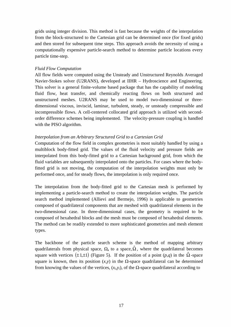
Fluid Flow Computation All flow fields were computed using the Unsteady and Unstructured Reynolds Averaged Navier-Stokes solver (U2RANS), developed at IIHR – Hydroscience and Engineering. This solver is a general finite-volume based package that has the capability of modeling fluid flow, heat transfer, and chemically reacting flows on both structured and unstructured meshes. U2RANS may be used to model two-dimensional or three-dimensional viscous, inviscid, laminar, turbulent, steady, or unsteady compressible and incompressible flows. A cell-centered collocated grid approach is utilized with second-order difference schemes being implemented. The velocity-pressure coupling is handled with the PISO algorithm. Interpolation from an Arbitrary Structured Grid to a Cartesian Grid Computation of the flow field in complex geometries is most suitably handled by using a multiblock body-fitted grid. The values of the fluid velocity and pressure fields are interpolated from this body-fitted grid to a Cartesian background grid, from which the fluid variables are subsequently interpolated onto the particles. For cases where the body-fitted grid is not moving, the computation of the interpolation weights must only be performed once, and for steady flows, the interpolation is only required once. The interpolation from the body-fitted grid to the Cartesian mesh is performed by implementing a particle-search method to create the interpolation weights. The particle search method implemented (Allievi and Bermejo, 1996) is applicable to geometries composed of quadrilateral components that are meshed with quadrilateral elements in the two-dimensional case. In three-dimensional cases, the geometry is required to be composed of hexahedral blocks and the mesh must be composed of hexahedral elements. The method can be readily extended to more sophisticated geometries and mesh element types. The backbone of the particle search scheme is the method of mapping arbitrary quadrilaterals from physical space, Ω, to a space, Ω , where the quadrilateral becomes square with vertices ( )1,1 ±± (Figure 5). If the position of a point (p,q) in the Ω -space square is known, then its position (x,y) in the Ω-space quadrilateral can be determined from knowing the values of the vertices, (xi,yi), of the Ω-space quadrilateral according to

18

,

4

1

4

1

ii

ii

yy

xx

Φ=

Φ=

∑

∑ (51)

where the shape functions, iΦ , are given by

( )( )( )( )( )( )( )( )qp

qpqpqp

+−=Φ++=Φ−+=Φ−−=Φ

1141114111411141

4

3

2

1

(52)

for simple quadrilateral shapes. In order for this mapping scheme to be of use for interpolation, the inverse relationship giving the coordinates in the Ω -space when the physical coordinates (xp,yp) are known is needed. This relationship can be found by solving the non-linear system of equations given by (51) and (52) for (p,q) using an iterative Newton-Raphson method. This gives

⎪⎭

⎪⎬⎫

⎪⎩

⎪⎨⎧

−

−

⎥⎥⎦

⎤

+

−−

⎢⎢⎣

⎡

−−

+∆

+⎪⎭

⎪⎬⎫

⎪⎩

⎪⎨⎧

=⎪⎭

⎪⎬⎫

⎪⎩

⎪⎨⎧

+

+

kpp

kpp

k

k

kq

k

kk

k

k

k

yy

xx

qaa

paaqbb

pbb

qp

qp

31

32

3

32

1

1 1 , (53)

where

( ) ( )( ) ( )( ) ( )( ) ( )( ) ( ) ( ) .

,,,

,,

322313311221

432141

3432141

3

241341

2241341

2

431241

1431241

1

4

1

4

1

kkk

ikk

iikpi

kkii

kp

qbabapbabababa

xxxxbxxxxaxxxxbxxxxayyyybxxxxa

qpyyqpxx

−+−+−=∆

−+−=−+−=−+−=−+−=−+−=−+−=

Φ=Φ= ∑∑ ==

(54)

The Cartesian mesh on which the particles are tracked is created in a manner such that it is rectangular and contains all of the complicated geometry (Figure 6). To determine in which block a Cartesian grid point is located, (53) and (54) are solved to find the value (p,q) which corresponds to the Cartesian point (xc,yc), where the quadrilateral vertices are taken as the grid-block vertices. If the point is in the block, the condition

1111

≤≤−≤≤−

qp

(55)

19

must hold. If this condition does not hold, the next block is examined. If the condition is not satisfied for any block, the point is outside the complicated geometry, and no further operations are performed for that point, and all variable values are set to zero.

Figure 5. A schematic of the mapping utilized to simplify the element search for the location of a Cartesian grid point in a complex mesh (from Allievi and Bermejo, 1997).

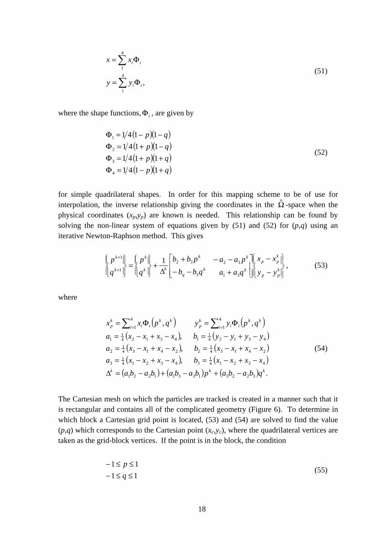
Figure 6. A Cartesian background mesh (blue) overlapped onto a block structured mesh for a converging-diverging nozzle flow.

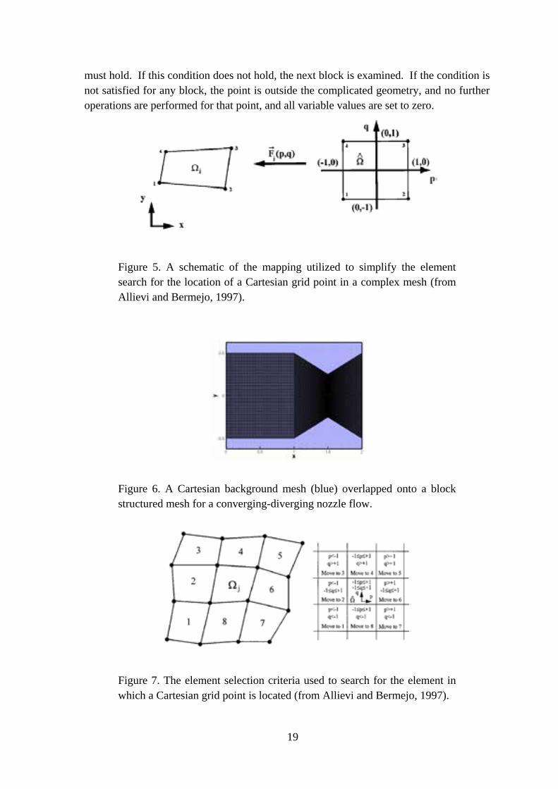
Figure 7. The element selection criteria used to search for the element in which a Cartesian grid point is located (from Allievi and Bermejo, 1997).

20

Once the block in which the Cartesian grid point is located is known, the particular element of the block in which the Cartesian point is located is determined. This is done in a manner similar to determining which block the point is in. Expression (53) is used to determine the values of p and q for a particular element where the element vertices are used as the quadrilateral vertices. If the condition given by (55) is satisfied the element contains the Cartesian point. If (55) is not satisfied, the next element is picked based on the values of p and q of the current element. This selection scheme is given in Figure 25, where the central element in the figure is the previously examined element that did not satisfy (55). The method moves from element to element in a rational manner until the correct element is found. Once the element is known, the interpolation weights can be formed in the Ω -space according to

( )

2/)1(2/1

+=+=

qp

ζξ

, (56)

where, ξ and ζ are the interpolation weights in the x- and y-direction. Both the appropriate element required for interpolation as well as the interpolation weights are stored. Once this information is computed, interpolation is straightforward. The methodology for computing the interpolation weights in three-dimensions is the same as the two-dimensional method. The only difference is one requires a mapping scheme for hexahedrals in place of quadrilaterals, but formulation of this mapping is straightforward. Representation of Embedded Boundaries on a Cartesian Grid In order to make interpolation of fluid forces onto the particles efficient, a Cartesian mesh is overlapped onto the body-fitted grid. This makes it simple to determine the particle locations, but it makes it necessary to somehow represent the now internal boundaries that form the geometry’s walls. To represent these boundaries, the value of the normal distance of a Cartesian point to the nearest surface is stored at each point in a band of points within a distance of 20 x∆ from the surfaces, where x∆ is the average of the grid-spacing in all coordinate directions. This field of normal distances is often known as a level-set function. The level-set value is interpolated onto the particles in the same manner as the fluid variables. If the level-set value at the particle center is less than a particle radius, the particle is determined as colliding with a wall. The level-set value is also used in determining whether to include a surface in a particle's local-list. Because of the adjustable size of the local-list, it is of value to know the value of the level-set function up to an arbitrary distance from a particular surface. The method used to compute this value for the each point in the Cartesian mesh is now discussed. The level-set function is often chosen to be a signed distance function (Sethian, 2001), and thus must satisfy

21

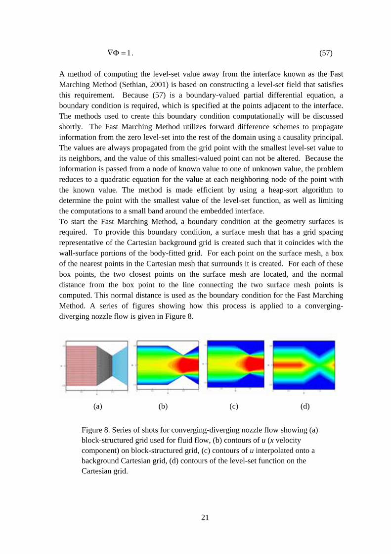
1=Φ∇ . (57) A method of computing the level-set value away from the interface known as the Fast Marching Method (Sethian, 2001) is based on constructing a level-set field that satisfies this requirement. Because (57) is a boundary-valued partial differential equation, a boundary condition is required, which is specified at the points adjacent to the interface. The methods used to create this boundary condition computationally will be discussed shortly. The Fast Marching Method utilizes forward difference schemes to propagate information from the zero level-set into the rest of the domain using a causality principal. The values are always propagated from the grid point with the smallest level-set value to its neighbors, and the value of this smallest-valued point can not be altered. Because the information is passed from a node of known value to one of unknown value, the problem reduces to a quadratic equation for the value at each neighboring node of the point with the known value. The method is made efficient by using a heap-sort algorithm to determine the point with the smallest value of the level-set function, as well as limiting the computations to a small band around the embedded interface. To start the Fast Marching Method, a boundary condition at the geometry surfaces is required. To provide this boundary condition, a surface mesh that has a grid spacing representative of the Cartesian background grid is created such that it coincides with the wall-surface portions of the body-fitted grid. For each point on the surface mesh, a box of the nearest points in the Cartesian mesh that surrounds it is created. For each of these box points, the two closest points on the surface mesh are located, and the normal distance from the box point to the line connecting the two surface mesh points is computed. This normal distance is used as the boundary condition for the Fast Marching Method. A series of figures showing how this process is applied to a converging-diverging nozzle flow is given in Figure 8.

(a) (b) (c) (d)

Figure 8. Series of shots for converging-diverging nozzle flow showing (a) block-structured grid used for fluid flow, (b) contours of u (x velocity component) on block-structured grid, (c) contours of u interpolated onto a background Cartesian grid, (d) contours of the level-set function on the Cartesian grid.

22

III. Two-Dimensional Test Cases In this section the particle collision and aggregation under van der Waals adhesion are examined for two test cases, both of which assume that the spherical particles are restricted to move in the x-y plane. The first test case is for a straight channel flow with fully-developed velocity profile and periodic end boundary conditions. In this test, we examine the dynamic process by which aggregates interact with each other near the channel walls, leading to capture of particles by the wall. The second test case is for flow through nozzles of various contraction lengths. This case utilizes the interpolation and level-set method described in Section II.E for particle transport in flows with complex geometry. The computations examine the growth of aggregates and the build-up of particle bridges within regions with contracting flow lines. The two test cases are representative of the particle adhesion dynamics within the fully-developed part and within the entrance part of a radiator cooling channel, respectively. A. Channel Flow The computations are performed for fully-developed two-dimensional laminar channel flow, where the fluid flow is assumed to be unaffected by the particles. The particle transport is periodic over a channel length equal to five times the channel width. All computational results are made dimensionless using the channel width L and maximum fluid velocity U as the fluid length and velocity scales. The particles are initially placed on an array with approximately even spacing in all three directions. The initial velocity of the particles is set equal to the local fluid velocity, plus a random perturbation with uniform probability density and maximum value equal to 0.05. The transport of particles is controlled by a number of dimensionless parameters. For adhesionless flow, these parameters include the density ratio χ , the Stokes number St, the dimensionless particle diameter ε , the average particle concentration 0c , and an elasticity parameter 2/ UE pρλ ≡ . The values of these parameters are selected to be typical of dust (sandstone) particles in air flow through a small channel, such as a radiator channel. For this application, we have 3kg/m 2600≅pρ , 3kg/m 2.1≅fρ ,

skg/m 102 5 ⋅×≅ −µ , and GPa 10≅E . The characteristic air velocity is taken to be m/s5.0≅U , the channel width is mm1=L , and the particle diameter is m10 µ≅d .

The governing dimensionless parameters are computed as 4106.4 −×≅χ , 01.0=ε , and 36.0=St . The elasticity parameter has the value 61015×≅λ for this system; however,

this high value makes the computation stiff, necessitating an excessive number of collision time steps. In order to make the problem more manageable, we reduce the elasticity parameter to 410=λ . We have repeated a sample computation with elastic parameter values 410=λ and 310=λ , and found that the results for rate of wall capture of particles and average size of wall-attached aggregates are nearly identical, thus demonstrating that the adhesion process for small particles is not sensitive to value of elastic modulus. The ratio of time scales discussed in Section II (with 132 10 fff == )

23

yield ε/10/ =∆∆ Ptt and 5/2/ λ=∆∆ CP tt , for which we obtain 10/ =∆∆ Ptt and 40/ =∆∆ CP tt . The dimensionless fluid time step is set as 01.0=∆t . A typical

computation with 8000 particles is run out to 10,000 fluid time steps, requiring about 24 hours of CPU time and consuming about 5% of the memory on a standard Pentium 4 personal computer with 2 GB RAM, operated under Linux. The strength of van der Waals adhesion is characterized by the surface potential energy γ. Denoting by A the effective Hamaker constant for the interaction of particle 1 and particle/wall 2 through a fluid medium 3, we can write ))(( 3231 AAAAA −−= , (58) where iA denotes the Hamaker constant for a material interacting with a like material in a vacuum. If δ denotes the characteristic minimum separation distance of two particle surfaces in the contact region, the effective surface potential γ can be related to A by

23 24621

δπγ

δ

Adhh

A == ∫∞

, (59)

where 36/ hA π is the van der Waals force per unit area between two infinite plates separated by a distance h. The presence of a fluid medium between the particles modifies γ both by modification of the effective Hamaker constant A and by regularizing of the minimum distance δ between the particles. From a computational study of the elastohydrodynamic response of two colliding particles, Serayssol and Davis (1986) show that the minimum separation distance between two colliding particles scales as 5/22/3 )/2( EUd πµδ ≈ . This estimate is found by Serayssol and Davis (1986) not to change significantly with addition of adhesive forces between the surfaces. A dimensionless adhesion parameter is used to characterize the magnitude of particle adhesive force relative to the particle inertia, defined by

RUp

2ργφ = . (60)

A necessary condition for particle capture is that for a single particle attached to a wall, the fluid drag force is less than the critical force for particle sliding and the torque about the contact point imposed by the fluid force is less than the critical moment for particle rolling. However, as noted by Bergendahl and Grasso (2000), detachment of a single particle from a wall tends to first be accompanied by particle rolling, rather than sliding.

24

An expression for onset of rolling can be obtained using the expression (44) for the critical rolling moment, with 0aa ≅ , and the expression (2) for fluid drag, with 1≅f , yielding a criterion for the critical dimensionless wall velocity gradient as

Cyu

critw θ2<∂∂ , (61)

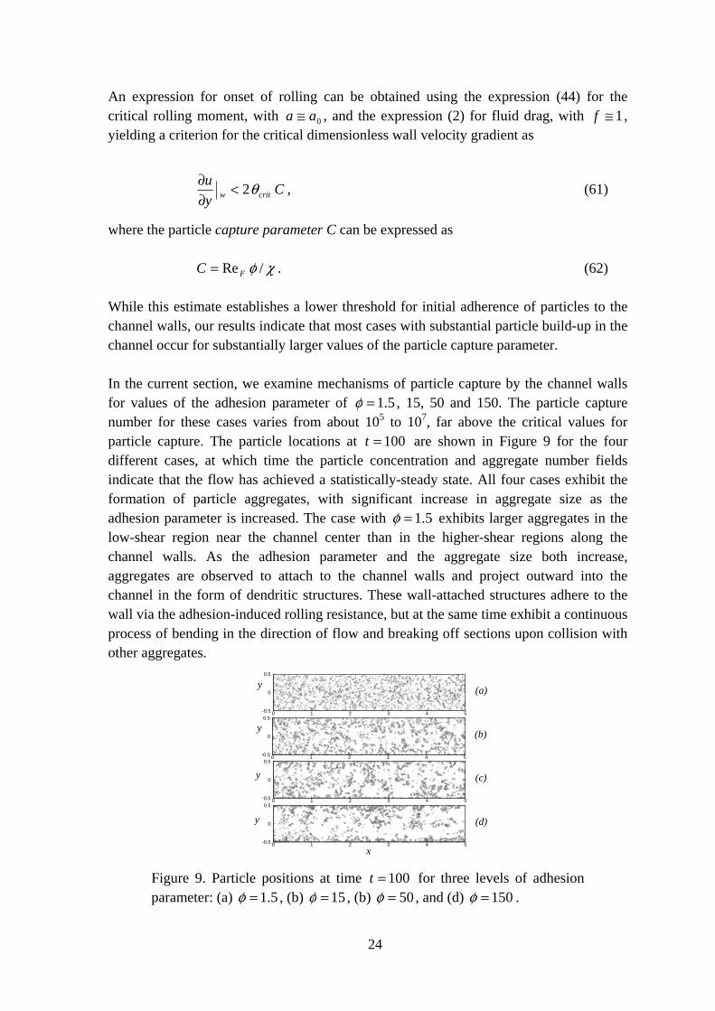
where the particle capture parameter C can be expressed as χφ /Re FC = . (62) While this estimate establishes a lower threshold for initial adherence of particles to the channel walls, our results indicate that most cases with substantial particle build-up in the channel occur for substantially larger values of the particle capture parameter. In the current section, we examine mechanisms of particle capture by the channel walls for values of the adhesion parameter of 5.1=φ , 15, 50 and 150. The particle capture number for these cases varies from about 105 to 107, far above the critical values for particle capture. The particle locations at 100=t are shown in Figure 9 for the four different cases, at which time the particle concentration and aggregate number fields indicate that the flow has achieved a statistically-steady state. All four cases exhibit the formation of particle aggregates, with significant increase in aggregate size as the adhesion parameter is increased. The case with 5.1=φ exhibits larger aggregates in the low-shear region near the channel center than in the higher-shear regions along the channel walls. As the adhesion parameter and the aggregate size both increase, aggregates are observed to attach to the channel walls and project outward into the channel in the form of dendritic structures. These wall-attached structures adhere to the wall via the adhesion-induced rolling resistance, but at the same time exhibit a continuous process of bending in the direction of flow and breaking off sections upon collision with other aggregates.

0 1 2 3 4 5-0.5

0

0.5

y

x

(d)

0 1 2 3 4 5-0.5

0

0.5

(c)y

0 1 2 3 4 5-0.5

0

0.5

(b)y0 1 2 3 4 5-0.5

0

0.5

(a)y

Figure 9. Particle positions at time 100=t for three levels of adhesion parameter: (a) 5.1=φ , (b) 15=φ , (b) 50=φ , and (d) 150=φ .

25

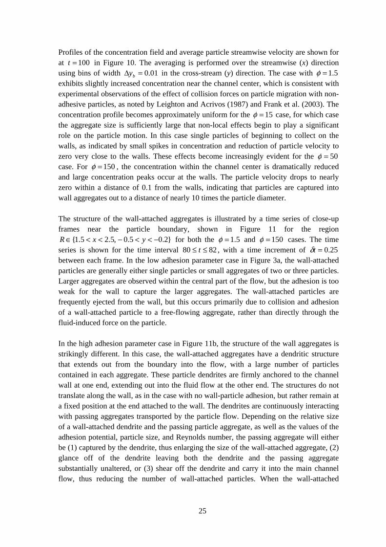
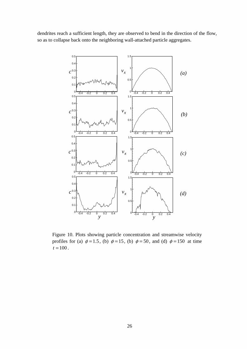
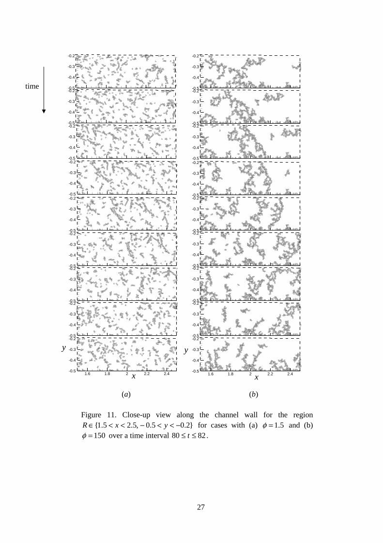
Profiles of the concentration field and average particle streamwise velocity are shown for at 100=t in Figure 10. The averaging is performed over the streamwise (x) direction using bins of width 01.0=∆ by in the cross-stream (y) direction. The case with 5.1=φ exhibits slightly increased concentration near the channel center, which is consistent with experimental observations of the effect of collision forces on particle migration with non-adhesive particles, as noted by Leighton and Acrivos (1987) and Frank et al. (2003). The concentration profile becomes approximately uniform for the 15=φ case, for which case the aggregate size is sufficiently large that non-local effects begin to play a significant role on the particle motion. In this case single particles of beginning to collect on the walls, as indicated by small spikes in concentration and reduction of particle velocity to zero very close to the walls. These effects become increasingly evident for the 50=φ case. For 150=φ , the concentration within the channel center is dramatically reduced and large concentration peaks occur at the walls. The particle velocity drops to nearly zero within a distance of 0.1 from the walls, indicating that particles are captured into wall aggregates out to a distance of nearly 10 times the particle diameter. The structure of the wall-attached aggregates is illustrated by a time series of close-up frames near the particle boundary, shown in Figure 11 for the region

2.05.0,5.25.1 −<<−<<∈ yxR for both the 5.1=φ and 150=φ cases. The time series is shown for the time interval 8280 ≤≤ t , with a time increment of 25.0=tδ between each frame. In the low adhesion parameter case in Figure 3a, the wall-attached particles are generally either single particles or small aggregates of two or three particles. Larger aggregates are observed within the central part of the flow, but the adhesion is too weak for the wall to capture the larger aggregates. The wall-attached particles are frequently ejected from the wall, but this occurs primarily due to collision and adhesion of a wall-attached particle to a free-flowing aggregate, rather than directly through the fluid-induced force on the particle. In the high adhesion parameter case in Figure 11b, the structure of the wall aggregates is strikingly different. In this case, the wall-attached aggregates have a dendritic structure that extends out from the boundary into the flow, with a large number of particles contained in each aggregate. These particle dendrites are firmly anchored to the channel wall at one end, extending out into the fluid flow at the other end. The structures do not translate along the wall, as in the case with no wall-particle adhesion, but rather remain at a fixed position at the end attached to the wall. The dendrites are continuously interacting with passing aggregates transported by the particle flow. Depending on the relative size of a wall-attached dendrite and the passing particle aggregate, as well as the values of the adhesion potential, particle size, and Reynolds number, the passing aggregate will either be (1) captured by the dendrite, thus enlarging the size of the wall-attached aggregate, (2) glance off of the dendrite leaving both the dendrite and the passing aggregate substantially unaltered, or (3) shear off the dendrite and carry it into the main channel flow, thus reducing the number of wall-attached particles. When the wall-attached

26

dendrites reach a sufficient length, they are observed to bend in the direction of the flow, so as to collapse back onto the neighboring wall-attached particle aggregates.

-0.4 -0.2 0 0.2 0.40

0.1

0.2

0.3

0.4

0.5

c

-0.4 -0.2 0 0.2 0.40

0.1

0.2

0.3

0.4

0.5

c

-0.4 -0.2 0 0.2 0.40

0.1

0.2

0.3

0.4

0.5

c

-0.4 -0.2 0 0.2 0.40

0.1

0.2

0.3

0.4

0.5

c

y

(a)

(b)

(c)

(d)

-0.4 -0.2 0 0.2 0.40

0.5

1

1.5

vx

-0.4 -0.2 0 0.2 0.40

0.5

1

1.5

vx

-0.4 -0.2 0 0.2 0.40

0.5

1

1.5

vx

-0.4 -0.2 0 0.2 0.40

0.5

1

1.5

v

y

x

Figure 10. Plots showing particle concentration and streamwise velocity profiles for (a) 5.1=φ , (b) 15=φ , (b) 50=φ , and (d) 150=φ at time

100=t .

27

-0.5

-0.4

-0.3

-0.2

-0.5

-0.4

-0.3

-0.2

-0.5

-0.4

-0.3

-0.2

-0.5

-0.4

-0.3

-0.2

-0.5

-0.4

-0.3

-0.2

-0.5

-0.4

-0.3

-0.2

-0.5

-0.4

-0.3

-0.2

-0.5

-0.4

-0.3

-0.2

1.6 1.8 2 2.2 2.4-0.5

-0.4

-0.3

-0.2

y

x

-0.5

-0.4

-0.3

-0.2

-0.5

-0.4

-0.3

-0.2

-0.5

-0.4

-0.3

-0.2

-0.5

-0.4

-0.3

-0.2

-0.5

-0.4

-0.3

-0.2

-0.5

-0.4

-0.3

-0.2

-0.5

-0.4

-0.3

-0.2

-0.5

-0.4

-0.3

-0.2

1.6 1.8 2 2.2 2.4-0.5

-0.4

-0.3

-0.2

x

y

(a) (b)

Figure 11. Close-up view along the channel wall for the region 2.05.0,5.25.1 −<<−<<∈ yxR for cases with (a) 5.1=φ and (b)

150=φ over a time interval 8280 ≤≤ t .

time

28

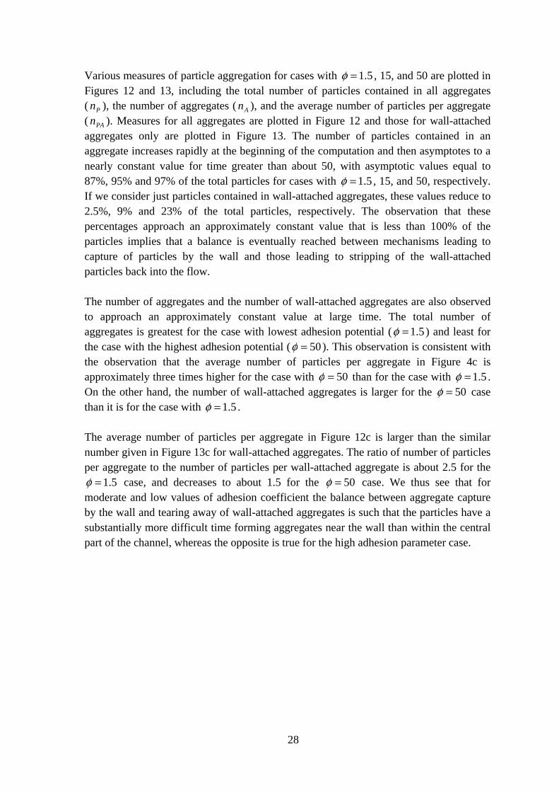
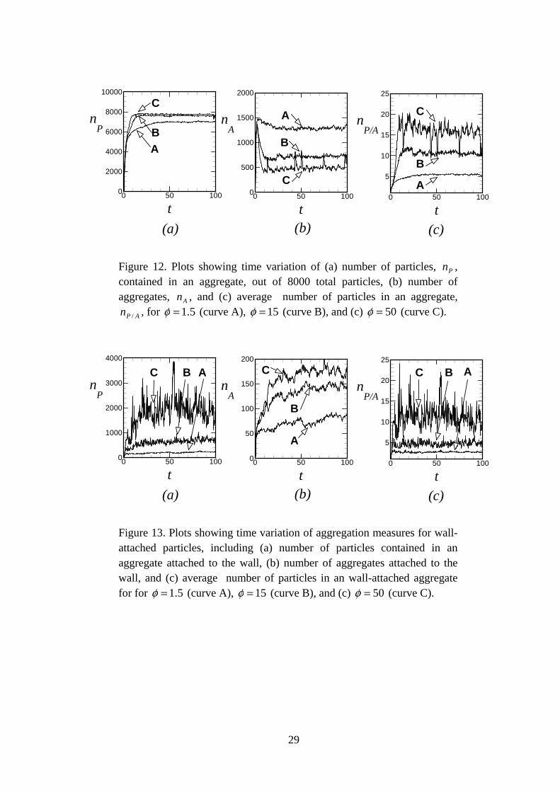
Various measures of particle aggregation for cases with 5.1=φ , 15, and 50 are plotted in Figures 12 and 13, including the total number of particles contained in all aggregates ( Pn ), the number of aggregates ( An ), and the average number of particles per aggregate ( PAn ). Measures for all aggregates are plotted in Figure 12 and those for wall-attached aggregates only are plotted in Figure 13. The number of particles contained in an aggregate increases rapidly at the beginning of the computation and then asymptotes to a nearly constant value for time greater than about 50, with asymptotic values equal to 87%, 95% and 97% of the total particles for cases with 5.1=φ , 15, and 50, respectively. If we consider just particles contained in wall-attached aggregates, these values reduce to 2.5%, 9% and 23% of the total particles, respectively. The observation that these percentages approach an approximately constant value that is less than 100% of the particles implies that a balance is eventually reached between mechanisms leading to capture of particles by the wall and those leading to stripping of the wall-attached particles back into the flow. The number of aggregates and the number of wall-attached aggregates are also observed to approach an approximately constant value at large time. The total number of aggregates is greatest for the case with lowest adhesion potential ( 5.1=φ ) and least for the case with the highest adhesion potential ( 50=φ ). This observation is consistent with the observation that the average number of particles per aggregate in Figure 4c is approximately three times higher for the case with 50=φ than for the case with 5.1=φ . On the other hand, the number of wall-attached aggregates is larger for the 50=φ case than it is for the case with 5.1=φ . The average number of particles per aggregate in Figure 12c is larger than the similar number given in Figure 13c for wall-attached aggregates. The ratio of number of particles per aggregate to the number of particles per wall-attached aggregate is about 2.5 for the

5.1=φ case, and decreases to about 1.5 for the 50=φ case. We thus see that for moderate and low values of adhesion coefficient the balance between aggregate capture by the wall and tearing away of wall-attached aggregates is such that the particles have a substantially more difficult time forming aggregates near the wall than within the central part of the channel, whereas the opposite is true for the high adhesion parameter case.

29

(c)(b)(a)

0 50 1000

2000

4000

6000

8000

10000

n

t

P

AB

C

0 50 100

5

10

15

20

25

n

t

P/A

A

B

C

0 50 1000

500

1000

1500

2000

n

t

AA

B

C

Figure 12. Plots showing time variation of (a) number of particles, Pn , contained in an aggregate, out of 8000 total particles, (b) number of aggregates, An , and (c) average number of particles in an aggregate,

APn / , for 5.1=φ (curve A), 15=φ (curve B), and (c) 50=φ (curve C).

(c)(b)(a)

0 50 100

5

10

15

20

25

n

t

P/A

ABC

0 50 1000

50

100

150

200

n

t

A

A

B

C

0 50 1000

1000

2000

3000

4000

n

t

P

ABC

Figure 13. Plots showing time variation of aggregation measures for wall-attached particles, including (a) number of particles contained in an aggregate attached to the wall, (b) number of aggregates attached to the wall, and (c) average number of particles in an wall-attached aggregate for for 5.1=φ (curve A), 15=φ (curve B), and (c) 50=φ (curve C).

30

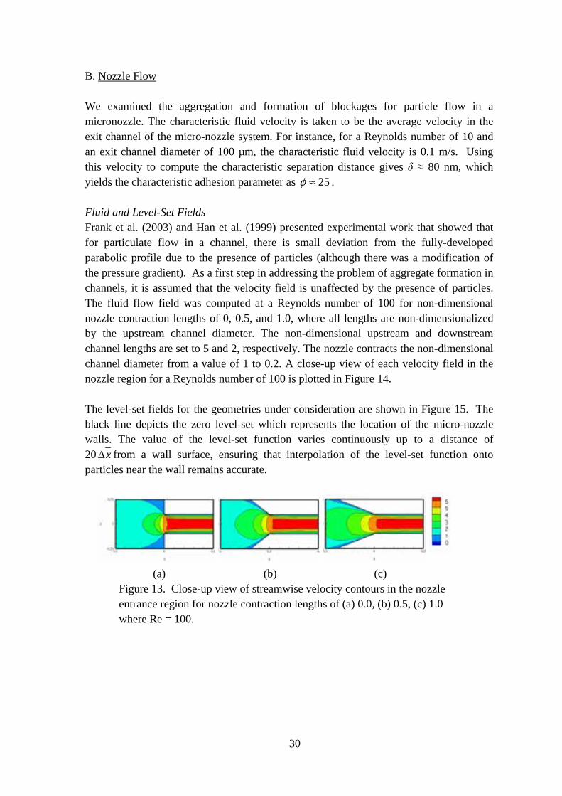
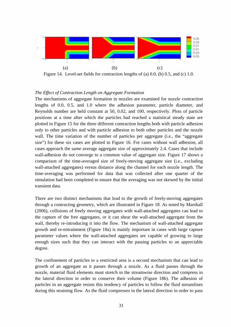
B. Nozzle Flow We examined the aggregation and formation of blockages for particle flow in a micronozzle. The characteristic fluid velocity is taken to be the average velocity in the exit channel of the micro-nozzle system. For instance, for a Reynolds number of 10 and an exit channel diameter of 100 µm, the characteristic fluid velocity is 0.1 m/s. Using this velocity to compute the characteristic separation distance gives δ ≈ 80 nm, which yields the characteristic adhesion parameter as 25≈φ . Fluid and Level-Set Fields Frank et al. (2003) and Han et al. (1999) presented experimental work that showed that for particulate flow in a channel, there is small deviation from the fully-developed parabolic profile due to the presence of particles (although there was a modification of the pressure gradient). As a first step in addressing the problem of aggregate formation in channels, it is assumed that the velocity field is unaffected by the presence of particles. The fluid flow field was computed at a Reynolds number of 100 for non-dimensional nozzle contraction lengths of 0, 0.5, and 1.0, where all lengths are non-dimensionalized by the upstream channel diameter. The non-dimensional upstream and downstream channel lengths are set to 5 and 2, respectively. The nozzle contracts the non-dimensional channel diameter from a value of 1 to 0.2. A close-up view of each velocity field in the nozzle region for a Reynolds number of 100 is plotted in Figure 14. The level-set fields for the geometries under consideration are shown in Figure 15. The black line depicts the zero level-set which represents the location of the micro-nozzle walls. The value of the level-set function varies continuously up to a distance of 20 x∆ from a wall surface, ensuring that interpolation of the level-set function onto particles near the wall remains accurate.

(a) (b) (c)

Figure 13. Close-up view of streamwise velocity contours in the nozzle entrance region for nozzle contraction lengths of (a) 0.0, (b) 0.5, (c) 1.0 where Re = 100.

31

(a) (b) (c)

Figure 14. Level-set fields for contraction lengths of (a) 0.0, (b) 0.5, and (c) 1.0.

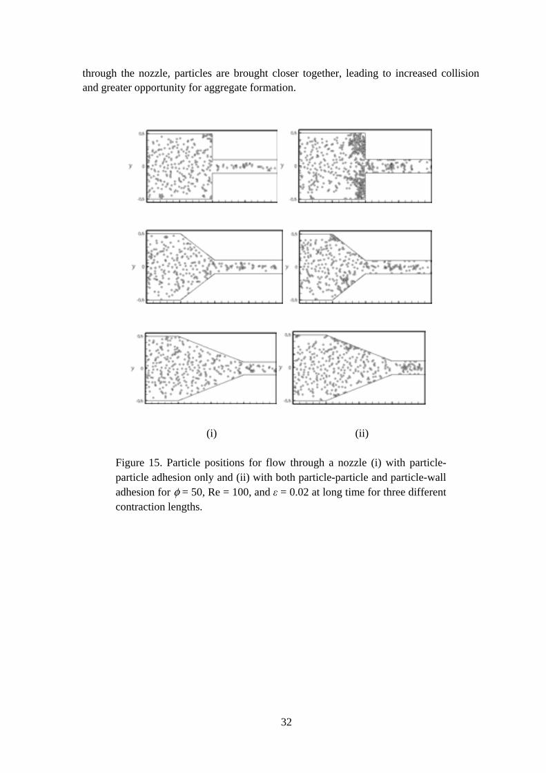
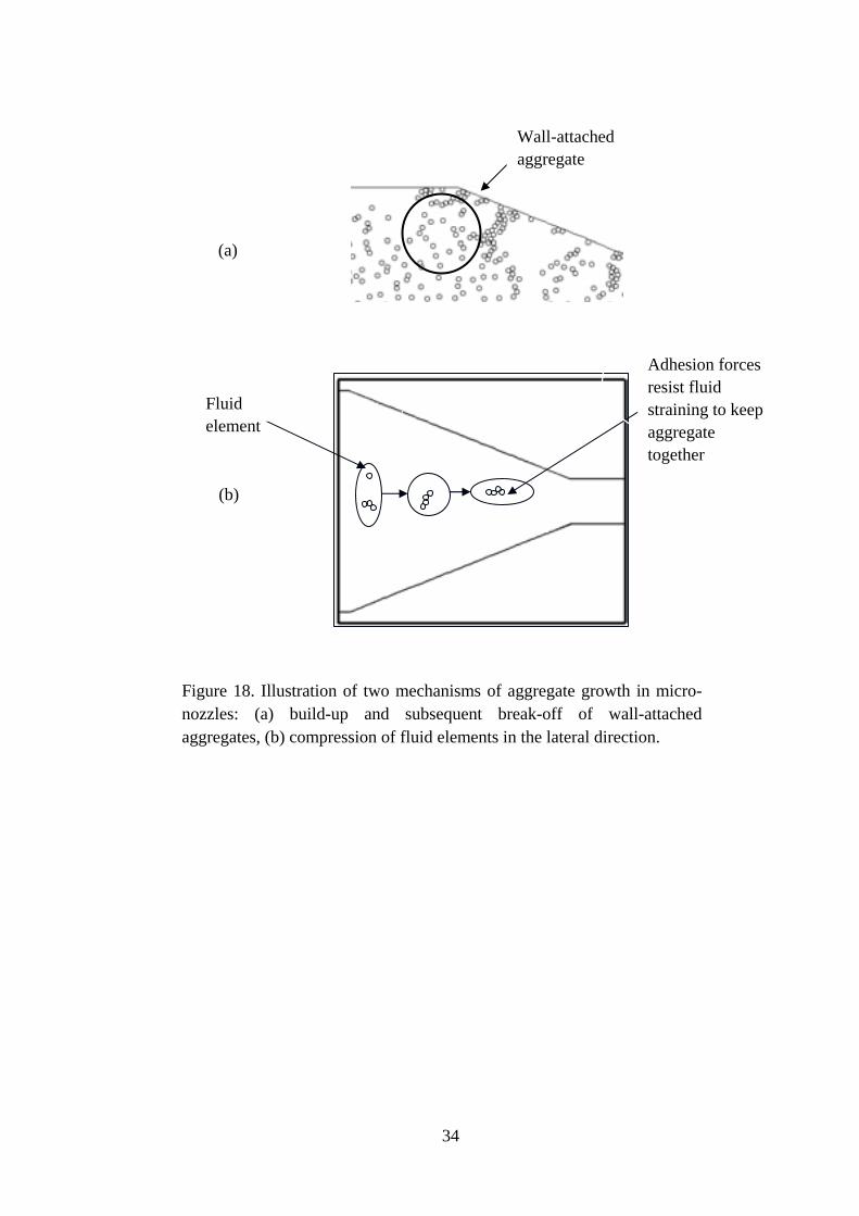
The Effect of Contraction Length on Aggregate Formation The mechanisms of aggregate formation in nozzles are examined for nozzle contraction lengths of 0.0, 0.5, and 1.0 where the adhesion parameter, particle diameter, and Reynolds number are held constant at 50, 0.02, and 100, respectively. Plots of particle positions at a time after which the particles had reached a statistical steady state are plotted in Figure 15 for the three different contraction lengths both with particle adhesion only to other particles and with particle adhesion to both other particles and the nozzle wall. The time variation of the number of particles per aggregate (i.e., the “aggregate size”) for these six cases are plotted in Figure 16. For cases without wall adhesion, all cases approach the same average aggregate size of approximately 2.4. Cases that include wall-adhesion do not converge to a common value of aggregate size. Figure 17 shows a comparison of the time-averaged size of freely-moving aggregate size (i.e., excluding wall-attached aggregates) versus distance along the channel for each nozzle length. The time-averaging was performed for data that was collected after one quarter of the simulation had been completed to ensure that the averaging was not skewed by the initial transient data. There are two distinct mechanisms that lead to the growth of freely-moving aggregates through a contracting geometry, which are illustrated in Figure 18. As noted by Marshall (2006), collisions of freely moving aggregates with wall-attached aggregates can lead to the capture of the free aggregates, or it can shear the wall-attached aggregate from the wall, thereby re-introducing it into the flow. The mechanism of wall-attached aggregate growth and re-entrainment (Figure 18a) is mainly important in cases with large capture parameter values where the wall-attached aggregates are capable of growing to large enough sizes such that they can interact with the passing particles to an appreciable degree. The confinement of particles to a restricted area is a second mechanism that can lead to growth of an aggregate as it passes through a nozzle. As a fluid passes through the nozzle, material fluid elements must stretch in the streamwise direction and compress in the lateral direction in order to conserve their volume (Figure 18b). The adhesion of particles in an aggregate resists this tendency of particles to follow the fluid streamlines during this straining flow. As the fluid compresses in the lateral direction in order to pass

32

through the nozzle, particles are brought closer together, leading to increased collision and greater opportunity for aggregate formation.

(i) (ii)

Figure 15. Particle positions for flow through a nozzle (i) with particle-particle adhesion only and (ii) with both particle-particle and particle-wall adhesion for φ = 50, Re = 100, and ε = 0.02 at long time for three different contraction lengths.

33

(a) (b)

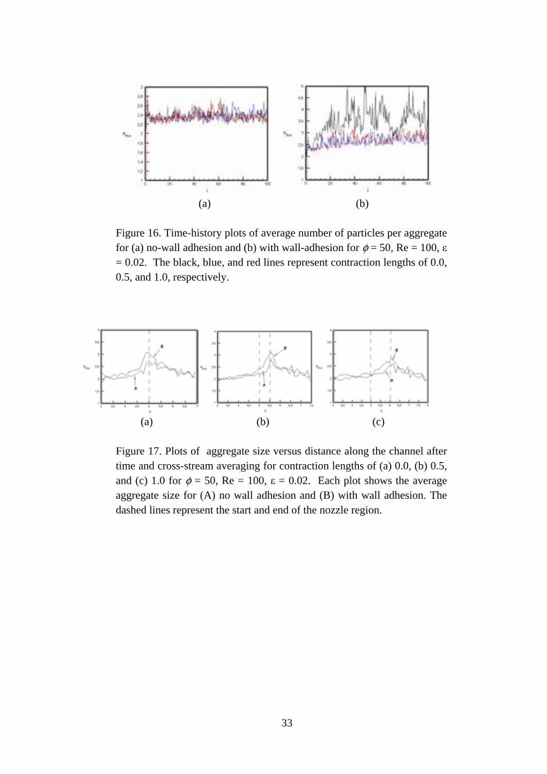
Figure 16. Time-history plots of average number of particles per aggregate for (a) no-wall adhesion and (b) with wall-adhesion for φ = 50, Re = 100, ε = 0.02. The black, blue, and red lines represent contraction lengths of 0.0, 0.5, and 1.0, respectively.

(a) (b) (c)

Figure 17. Plots of aggregate size versus distance along the channel after time and cross-stream averaging for contraction lengths of (a) 0.0, (b) 0.5, and (c) 1.0 for φ = 50, Re = 100, ε = 0.02. Each plot shows the average aggregate size for (A) no wall adhesion and (B) with wall adhesion. The dashed lines represent the start and end of the nozzle region.

34

Figure 18. Illustration of two mechanisms of aggregate growth in micro-nozzles: (a) build-up and subsequent break-off of wall-attached aggregates, (b) compression of fluid elements in the lateral direction.

Material

Element

Fluid Element Fluid element

Adhesion forces resist fluid straining to keep aggregate together

(b)

Wall-attached aggregate

(a)

35

Effects of Adhesion Parameter The effect of adhesion parameter on the formation of freely-moving aggregates is examined for adhesion parameter values of 25, 50, and 125. The contraction length, particle size, and Reynolds number are held constant at 1.0, 0.02, and 100, respectively. As the particle capture parameter C is a product of the adhesion parameter and Reynolds number, increasing the adhesion parameter while holding the Reynolds number constant would result in similar results to cases where the Reynolds number is increased while the adhesion parameter is held constant for a given value of the particle capture parameter. Figures 19 plots particle positions after the system has approached a statistical equilibrium for cases with φ = 25, 50, and 125. Figure 20 shows a comparison of the time-averaged size of freely-moving aggregates versus distance along the channel for the three adhesion parameters. Line plots for φ = 250 were not included, as this case lead to clogging of the channel which results in an unbounded growth of the aggregate size. All cases approach a state where the average aggregate size becomes statistically steady. The case with the highest adhesion parameter exhibits large fluctuations in the average aggregate size due to the increased growth and intermittent break-up of the wall-attached aggregates that can be attributed to the increase in the size of wall aggregates that results from the increased adhesion parameter. This intermittent ejection process creates new freely-moving aggregates that are typically larger than other freely-moving aggregates that have not originated in this manner. For φ = 25, most of the particles observed to be attached to the nozzle wall are single particles, not attached to any aggregate. These particles adhere to particles that pass near them, reducing the velocity of the recently attached particle such that it captures a small number of freely-moving particles. Once the newly formed particle chain grows to be 3-4 particles long, the chain either breaks and leaves 1-2 particles on the wall, or it bends over and deposits the particles on the wall. In this case, wall-attached aggregates inject new aggregates into the flow very infrequently. For very large adhesion parameters, wall-attached aggregates form on a larger portion of the nozzle walls, and these aggregates are considerably larger than the wall-attached aggregates formed for adhesion parameters of 25 and 50. The increased number of wall-attached aggregates leads to more frequent ejection of aggregates into the free-stream, as well as injection of larger aggregates. This increased injection of new freely-moving aggregates of large size causes the increase in the average aggregate size observed in Figure 20.

36

(a) (b) (c)

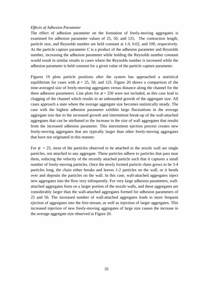
Figure 19. Particle positions for flow through a nozzle of unit length for adhesion parameter values (a) φ = 25, (b) φ = 50, and (c) φ = 125.

Figure 20. Plots of aggregate size versus distance along the channel after time and cross-stream averaging for a contraction length of 1.0, Re = 100, ε = 0.02, and Φ = (A) 25, (B) 50, and (C) 125. The dashed lines represent the start and end of the nozzle region.

Clogging in Micro-Nozzles For large capture parameter values, particle aggregation can lead to the formation of blockages in micro-nozzles. A qualitative examination of the mechanisms leading to nozzle blockage formation is performed in this section. After the blockage forms the particle blockages are likely to have a significant effect on the fluid flow. This effect is not yet included in our computations, but we propose to include it as part of the Phase II effort. Figure 21 shows particle positions for blockages in the nozzle for cases with three different contraction lengths. A time series showing the process by which these bridges develop is given in Figure 22 for the intermediate contraction length case. For contraction lengths of 0 and 0.5 the adhesion parameter was set to 125, and for the unity contraction geometry the adhesion parameter was 250. For all cases, the Reynolds number was 100, and the dimensionless particle diameter was 0.02. For these cases, the particle adhesion is sufficiently strong that large-size aggregates can grow attached to the nozzle wall. These wall-attached aggregates for long dendrites that

37

reach out into the flow and capture new particles. As the dendrite length increases, it begins to bend in the direction of flow due to the fluid forces. Particle bridges for when this process happens on both sides of the nozzle at the same time, such that two wall-attached dendrites on opposite sides of the nozzle bend toward the middle and impact each other at the nozzle centerline. The end particles of the dendrites attach to each other to form an arch-shaped bridge. Once formed, these bridges are sufficiently strong that they can withstand the fluid force as well as impact of upstream particles.

(a) (b) (c)

Figure 21. Nozzle clogging by particle bridges for cases with different contraction lengths for φ = 125, Re = 100, and ε = 0.02.

Figure 22. Time series illustrating clogging of a nozzle with a contraction length 0.5 and φ = 125, Re = 100, and ε = 0.02 with time increments of 1. The time series proceeds from top to bottom starting on the left.

38

IV. Three-Dimensional Test Cases A.. Pipe Flow In this section, we demonstrate the performance of the discrete-element method in three dimensions by examining the behavior of particles advected in a circular pipe flow with a parabolic laminar velocity profile. The fluid velocity at the pipe center and the pipe radius are used for the velocity and length scales, U and L, of the flow. The computational domain has length L4 with periodic boundary conditions at the two end planes. We use 5080 particles with effective radius 01.0/ =LR , which are initially evenly distributed within the pipe. The particle velocities are initialized to be the same as the fluid velocity, along with a random perturbation with zero mean and maximum deviation equal to U5.0 . The particle bulk concentration is 01.0=bulkc , defined as the ratio of the volume of particles to the total volume. The ratio of fluid to particle phase density is 01.0=χ , the pipe flow Reynolds number is 3000/Re == νULF , the particle Stokes number is 8.26=St , and the particle elasticity parameter is 176.0=λ . The particle restitution coefficient is set as 2.0=e , corresponding to damping coefficient

72.0=α . The flow is evolved using a fluid time step 1.0/ =∆ LtU , a particle time step ttP ∆=∆ 0263.0 , and a collision time step ttC ∆=∆ 00026.0 over a time interval from

)100,0(/ =LtU . There are, therefore, 3838 collision time steps and 38 particle time steps for each fluid time step. Computations both with no adhesion and with van der Waals adhesion are reported. Particle migration in pipe flow with no adhesion has been examined by a number of investigators, and two primary mechanisms have been identified that lead to lateral migration of particles. The first of these mechanisms is due to particle inertial effects, as incorporated in the lift and Magnus force terms discussed in Section 2 (Ho and Leal, 1974; Segre and Silberberg, 1962). For a circular pipe flow, the inertial forces cause the particles to be depleted from the pipe center and walls and to tend to collect near the radial location 6.0/ =Lr . The second mechanism for particle lateral transport is the shear-induced migration that arises from particle-particle collisions in the presence of fluid shear. Leighton and Acrivos (1987) showed that shear-induced migration causes particles to tend to migrate from regions of high to low particle concentration and from regions of high to low particle shear stress. Experimental studies of particle migration in a concentrated suspension are reported by Hampton et al. (1997) and Han et al. (1999) for flow in a circular tube and by Koh et al. (1994) for flow in a rectangular channel. These investigations note that whereas the inertial force tends to concentrate particles in circular pipe flow midway between the pipe center and the wall, the particle-particle collision forces tend to make the particles more concentrated in the low-shear region near the pipe center. For cases with small particle Reynolds number or high particle concentrations, the latter effect dominates and the particle concentrate peaks at the pipe center, whereas for cases with both large particle Reynolds numbers and low concentrations, a peak in particle concentration is observed near 6.0/ =Lr .

39

In computations with no adhesive force, the particle concentration field is averaged in both the axial and azimuthal directions. The particle concentration field is initially nearly uniform with radius (as shown by the dashed line in Figure 23), but as the computations proceed the concentration becomes higher in a region near the pipe center spanning the radii 5.0/05.0 << Lr and lower in the outer region spanning the radii 1/5.0 << Lr . An equilibrium configuration is approximately achieved by the final time, for which the concentration profile peaks to about 03.0=c at 2.0/ =Lr and decreases to about

008.0=c at 95.0/ =Lr , before plunging to nearly zero at the wall. The concentration value at 0=r tends to fluctuate significantly with time due to the small averaging volumes near the pipe center. The spatial fluctuations in Figure 23 have typical radial length scale of about 0.1, which is roughly ten times the grid size used for determination of the concentration field. Comparison of computations performed both with and without the lift and Magnus forces indicate that the inertial forces have a small effect on the computational results. Similarly, computations with different values of the restitution coefficient and the elastic modulus indicate that the results are not sensitive to the values of these parameters. The average number of particles involved in a collision ( CPn ) remains nearly constant at

02.002.2 ±=CPn during the computation, after a short initial transient. In Figure 24, we plot the total number of particles involved in collisions ( CPN ) and the number of distinct aggregates ( AN ) formed from these colliding particles. Both of these measures exhibit a steady decline during the computation as the average relative velocity between the particles and the surrounding fluid decreases. The same computation is now performed with the addition of van der Waals adhesion. Particle capture by surfaces was examined by Konstandopoulos (2000) using a “frozen deposit” assumption coupled with a hard-sphere model for the particle collisions. While this assumption may be appropriate for examining particle impact on a wall with no bulk fluid flow, in the presence of a fluid flow bending and break-up of the wall-attached aggregates is important in regulating the particle capture process. The average number of particles in an aggregate, plotted in Figure 25a, is found to increase from about 2.2 early in the computation to about 5.5 by the end of the computation. The total number of particles involved in a collision ( CPN ), plotted in Figure 25b, increases steadily during the computation, such that by 100/ =LtU approximately 80% of the particles are trapped in an aggregate. By contrast, the number of aggregates ( AN ) quickly increases to about 700 and then remains fairly constant for the remainder of the computation. The aggregate growth occurs both by capture of individual particles by aggregates and by collision of aggregates with small number of particles to form larger aggregates. The distribution of particles within aggregates of different sizes can be determined by plotting the total number of particles )( PAa nN contained within aggregates of size PAn , as shown in Figure 26. Most aggregates have relatively few particles (less than 10), but some aggregates are found with up to 60 particles.

40

Particle concentration and axial velocity profiles are shown in Figure 27 at a time

2/ =LtU near the start of the computation (dashed lines) and the final time ( 100/ =LtU ). The particle concentration is initially approximately uniform across the pipe. As the computation progresses, the particle concentration is found to attain a nearly constant value in a broad central region 8.0/0 << Lr , which decreases gradually with time. The particle concentration increases rapidly within a near-wall region

1/8.0 << Lr , with a peak in particle concentration at approximately 95.0/ =Lr . The spike in particle concentration near the wall is an outcome of particles trapped in aggregates that are then captured by van der Waals adhesion to the wall. Unlike the case with no adhesion, the particles trapped at the pipe wall generally exhibit no forward motion due to the rolling resistance associated with the van der Waals adhesion. For instance, the average particle velocity is plotted as a function of radius in Figure 27b for a time close to the start of the computation and for the final time. Near the start of the computation, the velocity profile approximately follows the parabolic profile of the fluid axial velocity, with some fluctuations that grow more pronounced near the pipe center. As the particle collect on the walls, however, the axial velocity exhibits an increasing decline near the wall, such that by 100/ =LtU the particle axial velocity vanishes for

Lr / greater than about 0.85.

0 0.2 0.4 0.6 0.8 10

0.01

0.02

0.03

c

r / L

(a) (b)

Figure 23. Plot showing (a) particle positions in pipe flow and (b) concentration profile at times 3/ =LtU (dashed line) and 100/ =LtU (solid line) for particle flow in a pipe with no adhesion force.

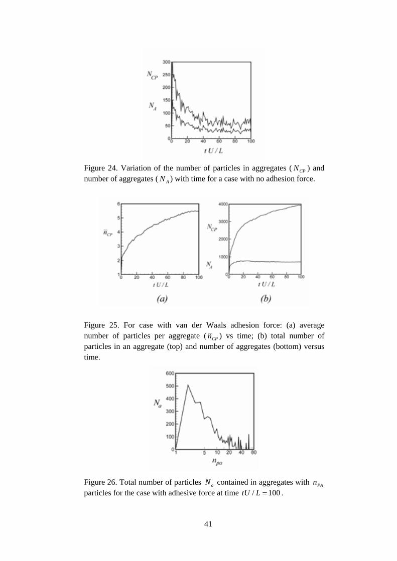
41

Figure 24. Variation of the number of particles in aggregates ( CPN ) and number of aggregates ( AN ) with time for a case with no adhesion force.

Figure 25. For case with van der Waals adhesion force: (a) average number of particles per aggregate ( CPn ) vs time; (b) total number of particles in an aggregate (top) and number of aggregates (bottom) versus time.

Figure 26. Total number of particles aN contained in aggregates with PAn particles for the case with adhesive force at time 100/ =LtU .

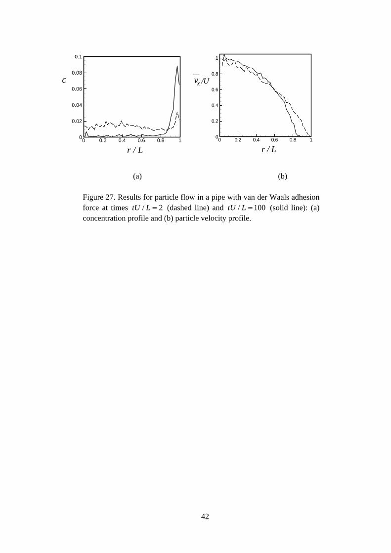
42

0 0.2 0.4 0.6 0.8 10

0.02

0.04

0.06

0.08

0.1

r / L

c

0 0.2 0.4 0.6 0.8 10

0.2

0.4

0.6

0.8

1

vx

__

r / L

/U

(a) (b)

Figure 27. Results for particle flow in a pipe with van der Waals adhesion force at times 2/ =LtU (dashed line) and 100/ =LtU (solid line): (a) concentration profile and (b) particle velocity profile.

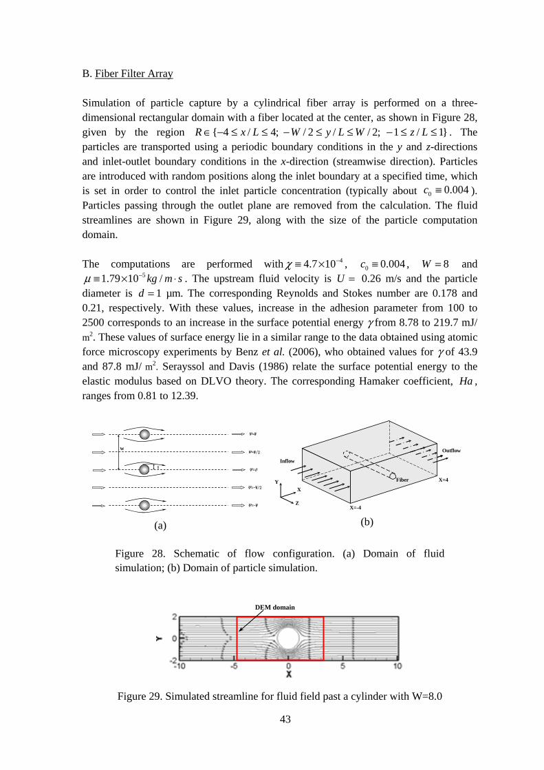
43

B. Fiber Filter Array Simulation of particle capture by a cylindrical fiber array is performed on a three-dimensional rectangular domain with a fiber located at the center, as shown in Figure 28, given by the region 1/1;2//2/;4/4 ≤≤−≤≤−≤≤−∈ LzWLyWLxR . The particles are transported using a periodic boundary conditions in the y and z-directions and inlet-outlet boundary conditions in the x-direction (streamwise direction). Particles are introduced with random positions along the inlet boundary at a specified time, which is set in order to control the inlet particle concentration (typically about 0 0.004c ≡ ). Particles passing through the outlet plane are removed from the calculation. The fluid streamlines are shown in Figure 29, along with the size of the particle computation domain. The computations are performed with 44.7 10χ −≡ × , 0 0.004c ≡ , 8=W and

51.79 10 /kg m sµ −≡ × ⋅ . The upstream fluid velocity is =U 0.26 m/s and the particle diameter is =d 1 µm. The corresponding Reynolds and Stokes number are 0.178 and 0.21, respectively. With these values, increase in the adhesion parameter from 100 to 2500 corresponds to an increase in the surface potential energy γ from 8.78 to 219.7 mJ/ m2. These values of surface energy lie in a similar range to the data obtained using atomic force microscopy experiments by Benz et al. (2006), who obtained values for γ of 43.9 and 87.8 mJ/ m2. Serayssol and Davis (1986) relate the surface potential energy to the elastic modulus based on DLVO theory. The corresponding Hamaker coefficient, Ha , ranges from 0.81 to 12.39.

1

W

Ψ=0

Ψ=W/2

Ψ=-W/2

Ψ=-W

Ψ=W

X

Z

Y

Outflow

Inflow

Fiber

X=-4

X=4

Figure 28. Schematic of flow configuration. (a) Domain of fluid simulation; (b) Domain of particle simulation.

Figure 29. Simulated streamline for fluid field past a cylinder with W=8.0

DEM domain

(a) (b)

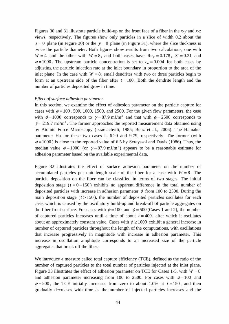
44

Figures 30 and 31 illustrate particle build-up on the front face of a fiber in the x-y and x-z views, respectively. The figures show only particles in a slice of width 0.2 about the

0=z plane (in Figure 30) or the 0=y plane (in Figure 31), where the slice thickness is twice the particle diameter. Both figures show results from two calculations, one with

4=W and the other with 8=W , and both cases have Re 0.178F = , 0.21St = and 1000φ = . The upstream particle concentration is set to 0 0.004c ≡ for both cases by

adjusting the particle injection rate at the inlet boundary in proportion to the area of the inlet plane. In the case with 8=W , small dendrites with two or three particles begin to form at an upstream side of the fiber after 100=t . Both the dendrite length and the number of particles deposited grow in time. Effect of surface adhesion parameter In this section, we examine the effect of adhesion parameter on the particle capture for cases with 100=φ , 500, 1000, 1500, and 2500. For the given flow parameters, the case with 1000φ = corresponds to 287.9 mJ/mγ = and that with 2500φ = corresponds to

2219.7 mJ/mγ = . The former approaches the reported measurement data obtained using by Atomic Force Microscopy (Israelachvili, 1985; Benz et al., 2006). The Hamaker parameter Ha for these two cases is 6.20 and 9.79, respectively. The former (with

1000φ = ) is close to the reported value of 6.5 by Serayssol and Davis (1986). Thus, the median value 1000=φ (or 287.9 mJ/mγ = ) appears to be a reasonable estimate for adhesion parameter based on the available experimental data. Figure 32 illustrates the effect of surface adhesion parameter on the number of accumulated particles per unit length scale of the fiber for a case with 8=W . The particle deposition on the fiber can be classified in terms of two stages. The initial deposition stage ( 1500 −=t ) exhibits no apparent difference in the total number of deposited particles with increase in adhesion parameter φ from 100 to 2500. During the main deposition stage ( 150>t ), the number of deposited particles oscillates for each case, which is caused by the oscillatory build-up and break-off of particle aggregates on the fiber front surface. For cases with 100φ = and 500φ = (Cases 1 and 2), the number of captured particles increases until a time of about 400=t , after which it oscillates about an approximately constant value. Cases with 1000≥φ exhibit a general increase in number of captured particles throughout the length of the computations, with oscillations that increase progressively in magnitude with increase in adhesion parameter. This increase in oscillation amplitude corresponds to an increased size of the particle aggregates that break off the fiber. We introduce a measure called total capture efficiency (TCE), defined as the ratio of the number of captured particles to the total number of particles injected at the inlet plane. Figure 33 illustrates the effect of adhesion parameter on TCE for Cases 1-5, with 8=W and adhesion parameter increasing from 100 to 2500. For cases with 100φ = and

500φ = , the TCE initially increases from zero to about 1.0% at 150=t , and then gradually decreases with time as the number of injected particles increases and the

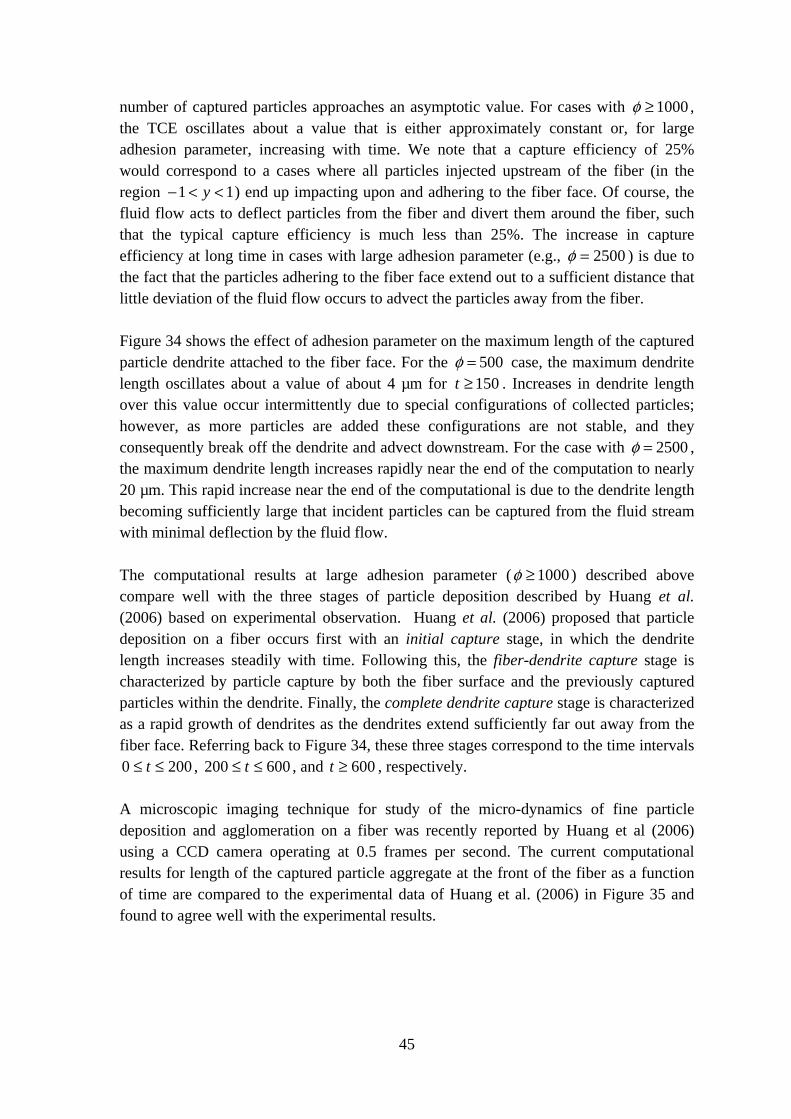
45

number of captured particles approaches an asymptotic value. For cases with 1000≥φ , the TCE oscillates about a value that is either approximately constant or, for large adhesion parameter, increasing with time. We note that a capture efficiency of 25% would correspond to a cases where all particles injected upstream of the fiber (in the region 11 <<− y ) end up impacting upon and adhering to the fiber face. Of course, the fluid flow acts to deflect particles from the fiber and divert them around the fiber, such that the typical capture efficiency is much less than 25%. The increase in capture efficiency at long time in cases with large adhesion parameter (e.g., 2500=φ ) is due to the fact that the particles adhering to the fiber face extend out to a sufficient distance that little deviation of the fluid flow occurs to advect the particles away from the fiber. Figure 34 shows the effect of adhesion parameter on the maximum length of the captured particle dendrite attached to the fiber face. For the 500φ = case, the maximum dendrite length oscillates about a value of about 4 µm for 150≥t . Increases in dendrite length over this value occur intermittently due to special configurations of collected particles; however, as more particles are added these configurations are not stable, and they consequently break off the dendrite and advect downstream. For the case with 2500φ = , the maximum dendrite length increases rapidly near the end of the computation to nearly 20 µm. This rapid increase near the end of the computational is due to the dendrite length becoming sufficiently large that incident particles can be captured from the fluid stream with minimal deflection by the fluid flow. The computational results at large adhesion parameter ( 1000≥φ ) described above compare well with the three stages of particle deposition described by Huang et al. (2006) based on experimental observation. Huang et al. (2006) proposed that particle deposition on a fiber occurs first with an initial capture stage, in which the dendrite length increases steadily with time. Following this, the fiber-dendrite capture stage is characterized by particle capture by both the fiber surface and the previously captured particles within the dendrite. Finally, the complete dendrite capture stage is characterized as a rapid growth of dendrites as the dendrites extend sufficiently far out away from the fiber face. Referring back to Figure 34, these three stages correspond to the time intervals

2000 ≤≤ t , 600200 ≤≤ t , and 600≥t , respectively. A microscopic imaging technique for study of the micro-dynamics of fine particle deposition and agglomeration on a fiber was recently reported by Huang et al (2006) using a CCD camera operating at 0.5 frames per second. The current computational results for length of the captured particle aggregate at the front of the fiber as a function of time are compared to the experimental data of Huang et al. (2006) in Figure 35 and found to agree well with the experimental results.

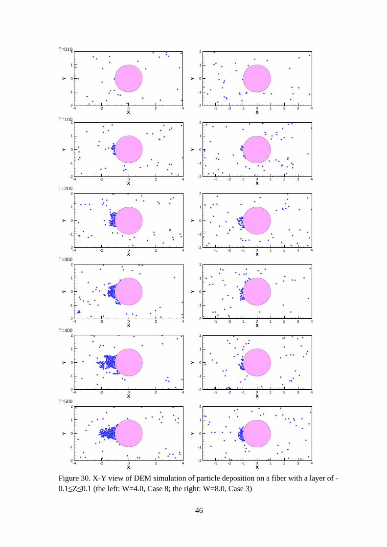
46

X

Y

-4 -2 0 2 4-2

-1

0

1

2

X

Y

-3 -2 -1 0 1 2 3 4-2

-1

0

1

2

X

Y

-4 -2 0 2 4-2

-1

0

1

2

X

Y

-3 -2 -1 0 1 2 3 4-2

-1

0

1

2

X

Y

-4 -2 0 2 4-2

-1

0

1

2

X

Y

-3 -2 -1 0 1 2 3 4-2

-1

0

1

2

X

Y

-4 -2 0 2 4-2

-1

0

1

2

X

Y

-3 -2 -1 0 1 2 3 4-2

-1

0

1

2

X

Y

-4 -2 0 2 4-2

-1

0

1

2

X

Y

-3 -2 -1 0 1 2 3 4-2

-1

0

1

2

X

Y

-4 -2 0 2 4-2

-1

0

1

2

X

Y

-3 -2 -1 0 1 2 3 4-2

-1

0

1

2

Figure 30. X-Y view of DEM simulation of particle deposition on a fiber with a layer of -0.1≤Z≤0.1 (the left: W=4.0, Case 8; the right: W=8.0, Case 3)

T=500

T=400

T=300

T=200

T=010

T=100

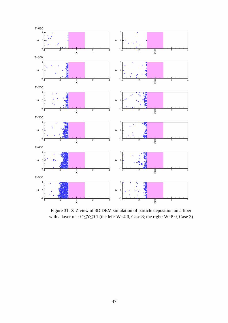
47

X

Z

-4 -2 0 2 4-1

0

1

X

Z

-4 -2 0 2 4-1

0

1

X

Z

-4 -2 0 2 4-1

0

1

X

Z

-4 -2 0 2 4-1

0

1

X

Z

-4 -2 0 2 4-1

0

1

XZ

-4 -2 0 2 4-1

0

1

X

Z

-4 -2 0 2 4-1

0

1

X

Z

-4 -2 0 2 4-1

0

1

X

Z

-4 -2 0 2 4-1

0

1

X

Z

-4 -2 0 2 4-1

0

1

X

Z

-4 -2 0 2 4-1

0

1

X

Z

-4 -2 0 2 4-1

0

1

Figure 31. X-Z view of 3D DEM simulation of particle deposition on a fiber

with a layer of -0.1≤Y≤0.1 (the left: W=4.0, Case 8; the right: W=8.0, Case 3)

T=500

T=400

T=300

T=200

T=010

T=100

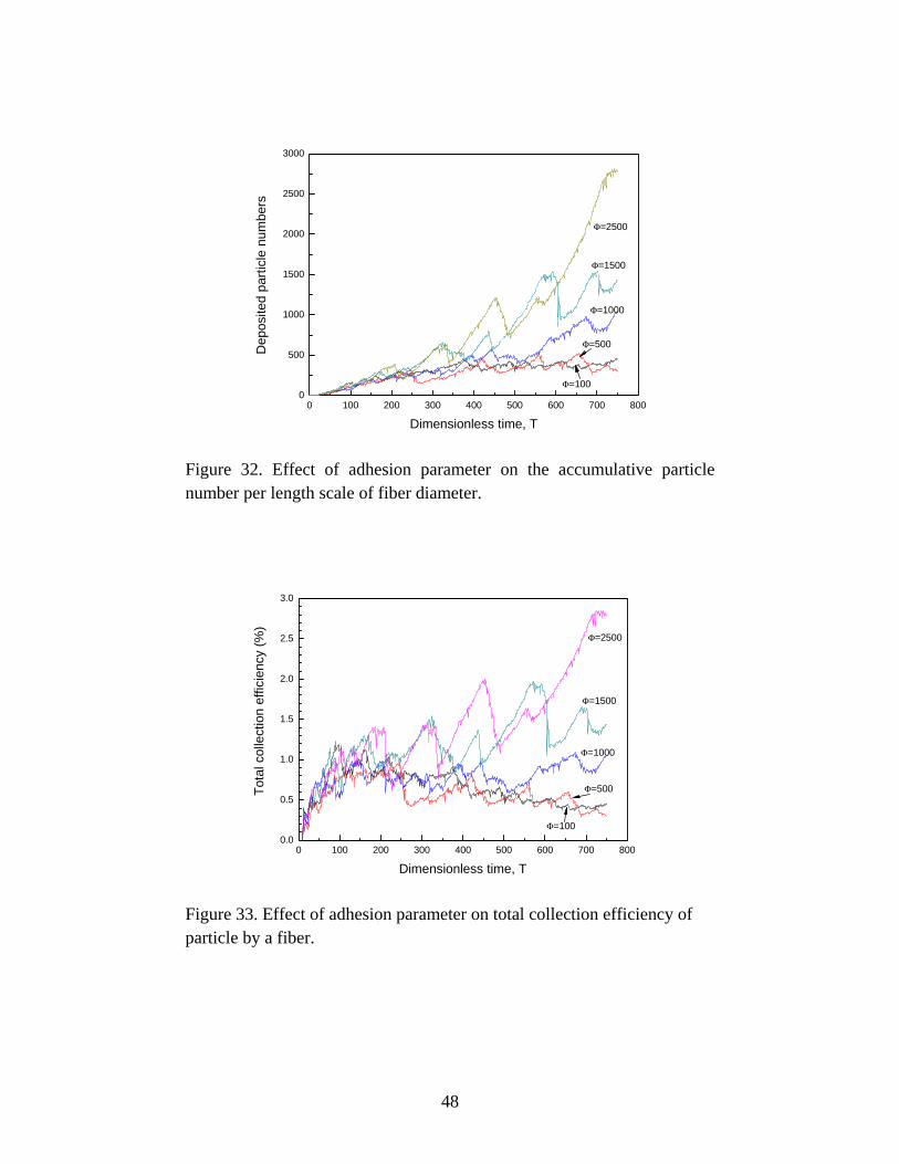
48

0 100 200 300 400 500 600 700 8000

500

1000

1500

2000

2500

3000

Φ=500

Φ=100

Φ=1000

Φ=1500

Dep

osite

d pa

rticl

e nu

mbe

rs

Dimensionless time, T

Φ=2500

Figure 32. Effect of adhesion parameter on the accumulative particle number per length scale of fiber diameter.

0 100 200 300 400 500 600 700 8000.0

0.5

1.0

1.5

2.0

2.5

3.0

Φ=100

Φ=500

Φ=1000

Φ=1500

Φ=2500

Tota

l col

lect

ion

effic

ienc

y (%

)

Dimensionless time, T

Figure 33. Effect of adhesion parameter on total collection efficiency of particle by a fiber.

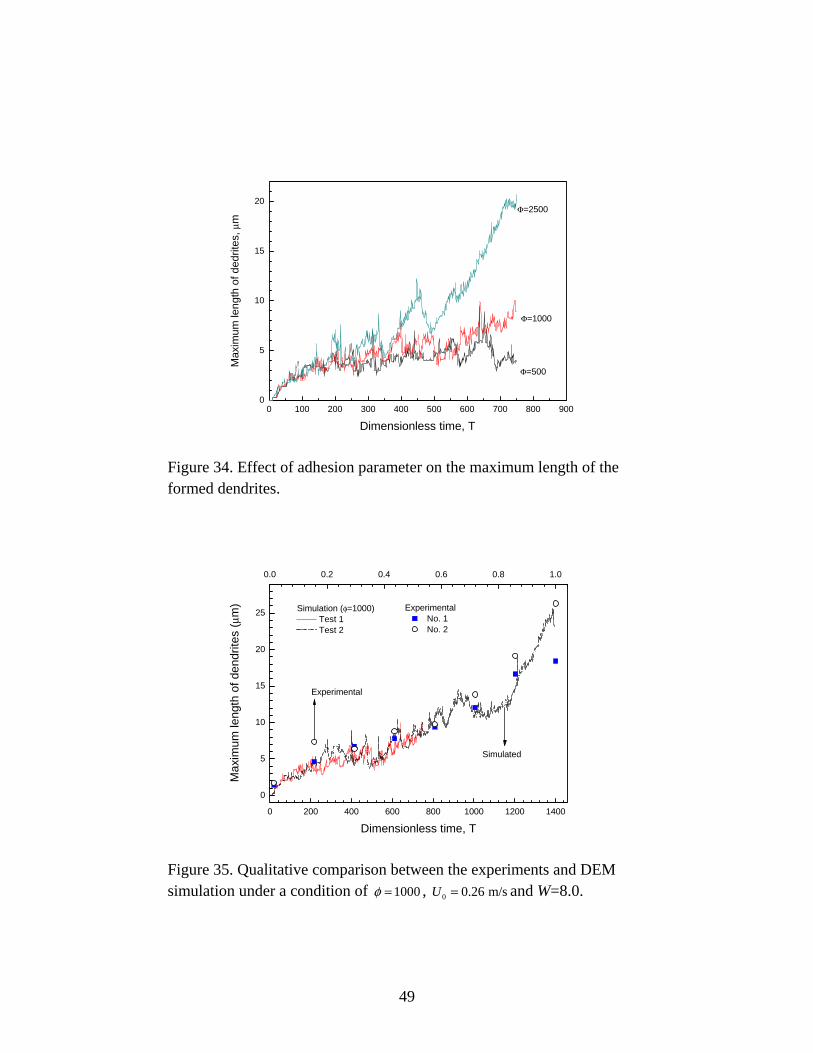
49

0 100 200 300 400 500 600 700 800 9000

5

10

15

20

Φ=500

Φ=1000

Φ=2500

Max

imum

leng

th o

f ded

rites

, µm

Dimensionless time, T

Figure 34. Effect of adhesion parameter on the maximum length of the formed dendrites.

0 200 400 600 800 1000 1200 1400

0

5

10

15

20

25

0.0 0.2 0.4 0.6 0.8 1.0

Simulation (φ=1000) Test 1 Test 2

Simulated

Max

imum

leng

th o

f den

drite

s (µ

m)

Dimensionless time, T

Experimental

Experimental No. 1 No. 2

Figure 35. Qualitative comparison between the experiments and DEM simulation under a condition of 1000φ = , 0 0.26 m/sU = and W=8.0.

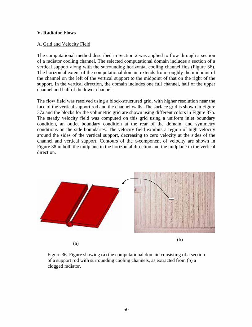
50

V. Radiator Flows A. Grid and Velocity Field The computational method described in Section 2 was applied to flow through a section of a radiator cooling channel. The selected computational domain includes a section of a vertical support along with the surrounding horizontal cooling channel fins (Figure 36). The horizontal extent of the computational domain extends from roughly the midpoint of the channel on the left of the vertical support to the midpoint of that on the right of the support. In the vertical direction, the domain includes one full channel, half of the upper channel and half of the lower channel. The flow field was resolved using a block-structured grid, with higher resolution near the face of the vertical support rod and the channel walls. The surface grid is shown in Figure 37a and the blocks for the volumetric grid are shown using different colors in Figure 37b. The steady velocity field was computed on this grid using a uniform inlet boundary condition, an outlet boundary condition at the rear of the domain, and symmetry conditions on the side boundaries. The velocity field exhibits a region of high velocity around the sides of the vertical support, decreasing to zero velocity at the sides of the channel and vertical support. Contours of the x-component of velocity are shown in Figure 38 in both the midplane in the horizontal direction and the midplane in the vertical direction.

(b) (a)

Figure 36. Figure showing (a) the computational domain consisting of a section of a support rod with surrounding cooling channels, as extracted from (b) a clogged radiator.

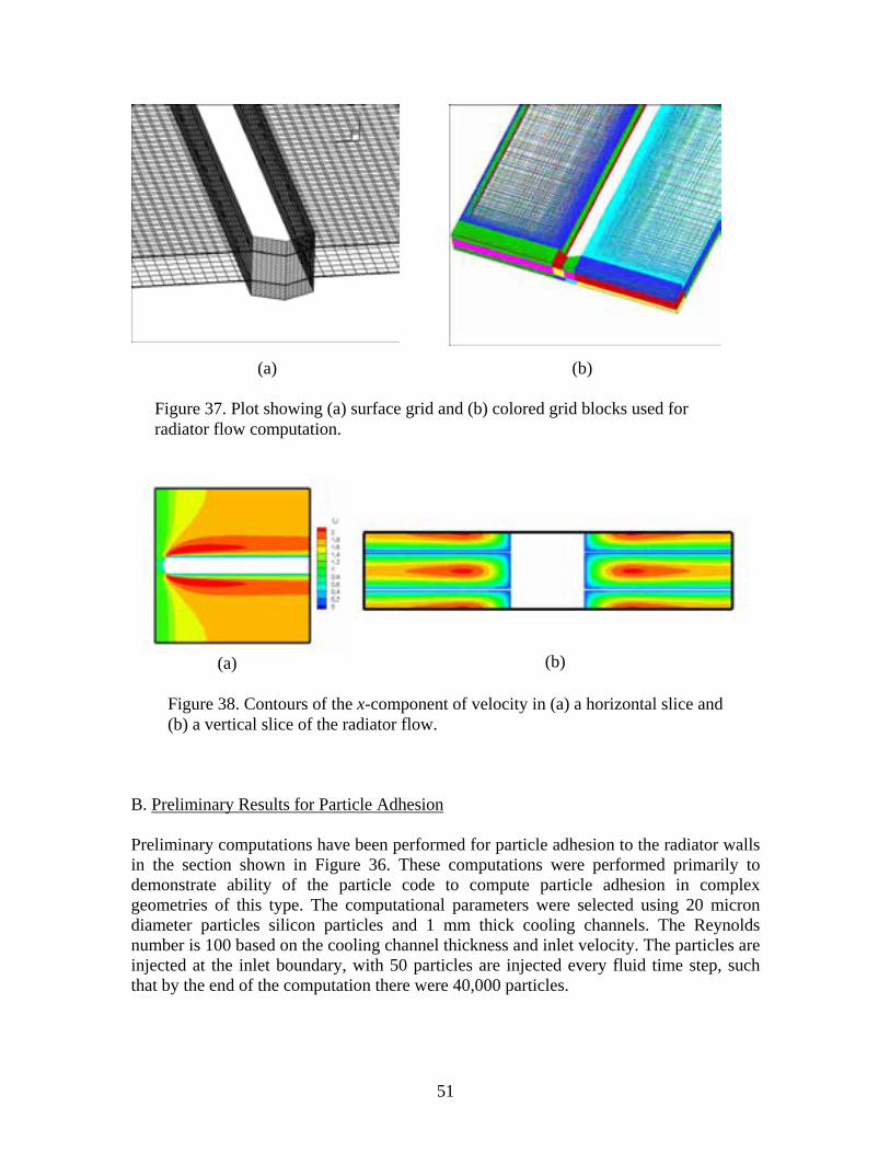
51

B. Preliminary Results for Particle Adhesion Preliminary computations have been performed for particle adhesion to the radiator walls in the section shown in Figure 36. These computations were performed primarily to demonstrate ability of the particle code to compute particle adhesion in complex geometries of this type. The computational parameters were selected using 20 micron diameter particles silicon particles and 1 mm thick cooling channels. The Reynolds number is 100 based on the cooling channel thickness and inlet velocity. The particles are injected at the inlet boundary, with 50 particles are injected every fluid time step, such that by the end of the computation there were 40,000 particles.

(a) (b)

Figure 37. Plot showing (a) surface grid and (b) colored grid blocks used for radiator flow computation.

(a) (b)

Figure 38. Contours of the x-component of velocity in (a) a horizontal slice and (b) a vertical slice of the radiator flow.

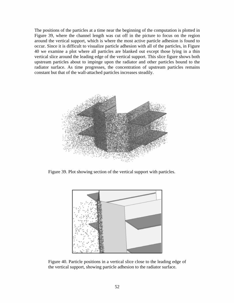
52

The positions of the particles at a time near the beginning of the computation is plotted in Figure 39, where the channel length was cut off in the picture to focus on the region around the vertical support, which is where the most active particle adhesion is found to occur. Since it is difficult to visualize particle adhesion with all of the particles, in Figure 40 we examine a plot where all particles are blanked out except those lying in a thin vertical slice around the leading edge of the vertical support. This slice figure shows both upstream particles about to impinge upon the radiator and other particles bound to the radiator surface. As time progresses, the concentration of upstream particles remains constant but that of the wall-attached particles increases steadily.

Figure 39. Plot showing section of the vertical support with particles.

Figure 40. Particle positions in a vertical slice close to the leading edge of the vertical support, showing particle adhesion to the radiator surface.

53

VII. References Cited Allievi, A. & Bermejo, R., “A generalized particle search-locate algorithm for arbitrary

grids,” Journal of Computational Physics 132, 157-166 (1997). Bagi, K. and Kuhn, M.R., “A definition of particle rolling in a granular assembly in terms

of particle translations and rotations,” Journal of Applied Mechanics 71, 493-501 (2004).

Bardet, J.P., “Observations on the effects of particle rotations on the failure of idealized

granular materials,” Mechanics of Materials 18(2), 159-182 (1994). Barnocky, G. and Davis, R.H., “The influence of pressure-dependent density and

viscosity on the elastohydrodynamic collision and rebound of two spheres,” Journal of Fluid Mechanics 209, 501-519 (1989).

Benz, M., Rosenberg, K.J., Kramer, E.J. and Israelachvili, J.N., “The Deformation and

Adhesion of Randomly Rough and Patterned Surfaces,” J. Phys. Chem. B 110, 11884-11893 (2006).

Bergendahl, J. and Grasso, D., “Prediction of colloid detachment in a model porous

media: hydrodynamics,” Chemical Engineering Science 55, 1523-1532 (2000). Brilliantov, N.V. and Pöschel, T., “Rolling as a ‘continuing collision’,” The European

Physics Journal B 12, 299-301 (1999). Brilliantov, N.V., Spahn, F., Hertzsch, J.-M., and Pöschel, T., “Model for collisions in

granular gases,” Physical Review E 53(5), 5382-5392 (1996). Burd, A.B. and Jackson, G.A., “Modeling steady-state particle size spectra,”

Environmental Science and Technology 36, 323-327 (2002). Chokshi, A., Tielens, A.G.G.M., and Hollenbach, D., “Dust coagulation,” The

Astrophysical Journal 407, 806-819 (1993). Cleary, P.W., Metcalfe, G. and Liffman, K., “How well do discrete element granular flow

models capture the essentials of mixing processes?,” Applied Mathematical Modeling 22, 995-1008 (1998).

Crowe, C.T., Sommerfeld, M. and Tsuji, Y., Multiphase Flows with Droplets and

Particles, CRC Press, Boca Raton (1998).

54

Cundall, P.A. and Strack, O.D.L., “A discrete numerical model for granular assembles,”

Geotechnique 29(1), 47-65 (1979). Davis, R.H., Serayssol, J.M. and Hinch, E.J., “The elastohydrodynamic collision of 2

spheres,” Journal of Fluid Mechanics 163, 479-497 (1986). Di Felice, R., “The voidage function for fluid-particle interaction systems,” International

Journal of Multiphase Flow 20, 153-159 (1994). Dominik, C. and Tielens, A.G.G.M., “Resistance to rolling in the adhesive contact of two

elastic spheres,” Philosophical Magazine A 92(3), 783-803 (1995). Dominik, C. and Tielens, A.G.G.M., “The physics of dust coagulation and the structure

of dust aggregates in space,” The Astrophysical Journal 480, 647-673 (1997). Druzhinin, O.A. and Ostrovsky, L.A., “The influence of Basset force on particle

dynamics in two-dimensional flows,” Physica D 76, 34-43 (1994). Frank, M., Anderson, D., Weeks, E.R. and Morris, J.F., “Particle migration in pressure-

driven flow of a Brownian suspension,” Journal of Fluid Mechanics 493, 363-378 (2003).

Hampton, R.E., Mammoli, A.A., Graham, A.L., Tetlow, N. and Altobelli, S.A.,

“Migration of particles undergoing pressure-driven flow in a circular conduit,” Journal of Rheology 41, 621-640 (1997).

Han, M., Kim, C., Kim, M. and Lee, S., “Particle migration in tube flow of suspensions,”

Journal of Rheology 43(5), 1157-1174 (1999). Hertz, H., “Über die Berührung fester elastische Körper,” J. reine und angewandte

Mathematik 92, 156-171 (1882). Ho, B.P. and Leal, L.G., “Inertial migration of rigid spheres in two-dimensional

unidirectional flows,” Journal of Fluid Mechanics 65, 365-400 (1974). Hu, K.C. and Mei, R., “Particle collision rate in fluid flows,” Physics of Fluids 10(4),

1028-1030 (1998).

55

Huang, B., Yaio, Q., Li, S.-Q., Zhao, H.-L., Song, Q. and You, C.-F., “Experimental investigation on the particle capture by a single fiber using microscopic image technique,” Powder Technology (2006)

Israelachvili, J., Intermolecular and Surface Forces, Academic Press, Amsterdam (1985). Iwashita, K. and Oda, M., “Rolling resistance at contacts in simulation of shear band

development by DEM,” Journal of Engineering Mechanics 124(3), 285-292 (1998). Johnson, K.L., Contact Mechanics, Cambridge University Press, Cambridge, U.K.

(1985). Johnson, K.L., Kendall, K. and Roberts, A.D., “Surface energy and the contact of elastic

solids,” Proceedings of the Royal Society of London A 324, 301-313 (1971). Koh, C.J., Hookham, P. and Leal, L.G., “An experimental investigation of concentrated

suspension flows in a rectangular channel,” Journal of Fluid Mechanics 266, 1-32 (1994).

Konstandopoulos, A., “Deposit growth dynamics: particle sticking and scattering

phenomena,” Powder Technology 109, 262-277 (2000). Kuhn, M.R. and Bagi, K., “Contact rolling and deformation in granular media,”

International Journal of Solids and Structures 41, 5793-5820 (2004). Leighton, D. and Acrivos, A., “The shear-induced migration of particles in concentrated

suspensions,” Journal of Fluid Mechanics 181, 415-439 (1987). Lian, G., Thornton, C. and Adams, M.J., “A theoretical study of the liquid bridge forces

between two rigid spherical bodies,” Journal of Colloid and Interface Science 161, 138-147 (1993).

Marshall, J.S., “Discrete-element modeling of particulate aerosol flows,” Journal of

Computational Physics (submitted) (2006a). Marshall, J.S., “Particle aggregation and capture by walls in a particulate aerosol channel

flow,” Journal of Aerosol Science (submitted) (2006b). Matthewson, M.J., “Adhesion of spheres by thin liquid films,” Philosophical Magazine A

57(2), 207-216 (1988).

56

Mehrotra, V.P. and Sastry, K.V.S., “Pendular bond strength between unequal-sized

spherical particles,” Powder Technology 25, 203-214 (1980). Mindlin, R.D., “Compliance of elastic bodies in contact,” Journal of Applied Mechanics

16, 259-268 (1949). Oda, M., Konishi, J. and Nemat-Nasser, S., “Experimental micromechanical evaluation

of strength of granular materials: effects of particle rolling,” Mechanics of Materials 1(4), 269-283 (1982).

Pitois, O., Moucheront, P. and Chateau, X., “Liquid bridge between two moving spheres:

An experimental study of viscosity effects,” Journal of Colloid and Interface Science 231, 26-31 (2000).

Pitois, O., Moucheront, P. and Chateau, X., “Rupture energy of a pendular bridge,”

European Physical Journal B 23, 79-86 (2001). Saffman, P.G., “The lift on a small sphere in a slow shear flow,” Journal of Fluid

Mechanics 22, 385-400 (1965). Saffman, P.G., “Corrigendum to 'The lift force on a small sphere in a slow shear flow',”

Journal of Fluid Mechanics 31, 624 (1968). Savkoor, A.R. and Briggs, G.A.D., “The effect of tangential force on the contact of

elastic solids in adhesion,” Proceedings of the Royal Society of London A 356, 103-114 (1977).

Segre, G. and Silberberg, A., “Behavior of macroscopic rigid spheres in Poiseuille flow.

Part 2. Experimental results and interpretation,” Journal of Fluid Mechanics 14, 136-157 (1962).

Serayssol, J.-M. and Davis, R.H., “The influence of surface interactions on the

elastohydrodynamic collision of two spheres,” Journal of Colloid and Interface Science 114(1), 54-66 (1986).

Sethian, J., Level Set Methods and Fast Marching Methods: Evolving Interfaces in

Computational Geometry, Fluid Mechanics, Computer Vision, and Materials Science, Cambridge University Press, Cambridge U.K. (2001).

57

Tabor, D., “The mechanism of rolling friction: the elastic range,” Proceedings of the Royal Society of London A 229, 198-220 (1955).

Thornton, C., “Interparticle sliding in the presence of adhesion,” Journal Physics D:

Applied Physics 24, 1942-1946 (1991). Thornton, C. and Yin, K.K., “Impact of elastic spheres with and without adhesion,”

Powder Technology 65, 153-166 (1991). Tsuji, Y., Tanaka, T. and Ishida, T., “Lagrangian numerical simulation of plug flow of

cohesionless particles in a horizontal pipe,” Powder Technology 71, 239-250 (1992). Visser, J., “Van der Waals and other cohesive forces affecting powder fluidization,”

Powder Technology 58, 1-10 (1989). VIII. List of Staff Working on Project Jeff Marshall, Professor, Mech. & Indust. Engr., University of Iowa, until July 2006

Professor & Director, School of Engr, Univ. Vermont, Aug 2006 - present John Mousel, M.S. student, University of Iowa, degree awarded December 2006. Shuiqing Li, Assistant Professor, Tsinghua University, China (visiting Univ. Iowa during

Summer 2006) IX. List of Papers and Theses A. Journal Articles Marshall, J.S., “Effect of shear-induced migration on the expulsion of heavy particles from a vortex core,” Physics of Fluids, Vol.18, No.11, 2006, pp. 113301-1 – 113301-12. Marshall, J.S., “Discrete-element modeling of particulate aerosol flows,” Journal of Computational Physics (submitted, 2006). Marshall, J.S., “Particle aggregation and capture by walls in a particulate aerosol channel flow,” Journal of Aerosol Science (submitted, 2006).

58

Mousel, J. and Marshall, J.S., “Particle aggregation in a microchannel nozzle flow,” in preparation. Mousel, J. and Marshall, J.S., “Particle wall adhesion for dusty gas flow in a radiator entrance region,” in preparation. Li, S.Q. and Marshall, J.S., “Discrete element simulation of particle deposition on a cylindrical fiber in an array,” in preparation. B. Thesis Mousel, J., “A computational investigation of particle aggregate growth in micro-nozzles using discrete-element modeling,” M.S. Thesis, University of Iowa, Iowa City, December (2006). C. Conferences Marshall, J.S., “Particulate aggregate formation and wall adhesion in microchannel flows,” ASME Joint U.S.-European Fluids Engineering Division Summer Meeting, Miami, Florida, July 17-20, 2006 (FEDSM2006-98117). Li, S.Q., Marshall, J.S., Ratner, A. and Yao, Q., “Granular dynamics simulation of particle deposition and coagulation in two-phase dilute flow,” 12th Conference of Engineering Thermophysics of China, Division of Combustion Institute, Wuhan, China, Nov., 2006. Mousel, J. and Marshall, J.S., “Particle aggregation and deposition in a micro-nozzle flow,” 56th Annual Meeting of the Fluid Dynamics Division of the American Physical Society (Bulletin of the American Physical Society, Vol. 51, No. 9, 2006), Tampa, Florida, Nov. 26-28, 2006.