Simulations of the mid-Pliocene Warm Period using two ... · Bab al-Mandab Connects Red Sea and Gulf of Aden 140 25000 parameterised parameterised Malacca Between Malay Peninsula

Geosci. Model Dev., 6, 517–531, 2013www.geosci-model-dev.net/6/517/2013/doi:10.5194/gmd-6-517-2013© Author(s) 2013. CC Attribution 3.0 License.

��Model Development

Open A

ccess

Simulations of the mid-Pliocene Warm Period using two versions ofthe NASA/GISS ModelE2-R Coupled ModelM. A. Chandler1,2, L. E. Sohl1,2, J. A. Jonas1,2, H. J. Dowsett3, and M. Kelley2,41Center for Climate Systems Research at Columbia University, New York, New York, USA2NASA Goddard Institute for Space Studies, New York, New York, USA3Eastern Geology & Paleoclimate Science Center, US Geological Survey, Reston, Virginia, USA4Trinnovim LLC, 2880 Broadway, New York, New York 10025, USA

Correspondence to:M. A. Chandler ([email protected])

Received: 31 July 2012 – Published in Geosci. Model Dev. Discuss.: 13 September 2012Revised: 14 March 2013 – Accepted: 21 March 2013 – Published: 24 April 2013

Abstract. The mid-Pliocene Warm Period (mPWP) bearsmany similarities to aspects of future global warming as pro-jected by the Intergovernmental Panel on Climate Change(IPCC, 2007). Both marine and terrestrial data point to high-latitude temperature amplification, including large decreasesin sea ice and land ice, as well as expansion of warmerclimate biomes into higher latitudes. Here we present ourmost recent simulations of the mid-Pliocene climate usingthe CMIP5 version of the NASA/GISS Earth System Model(ModelE2-R). We describe the substantial impact associatedwith a recent correction made in the implementation of theGent-McWilliams ocean mixing scheme (GM), which has alarge effect on the simulation of ocean surface temperatures,particularly in the North Atlantic Ocean. The effect of thiscorrection on the Pliocene climate results would not havebeen easily determined from examining its impact on thepreindustrial runs alone, a useful demonstration of how theconsequences of code improvements as seen in modern cli-mate control runs do not necessarily portend the impacts inextreme climates.Both the GM-corrected and GM-uncorrected simulations

were contributed to the Pliocene Model IntercomparisonProject (PlioMIP) Experiment 2. Many findings presentedhere corroborate results from other PlioMIP multi-modelensemble papers, but we also emphasise features in theModelE2-R simulations that are unlike the ensemble means.The corrected version yields results that more closely resem-ble the ocean core data as well as the PRISM3D reconstruc-tions of the mid-Pliocene, especially the dramatic warmingin the North Atlantic and Greenland-Iceland-Norwegian Sea,

which in the new simulation appears to be far more realis-tic than previously found with older versions of the GISSmodel. Our belief is that continued development of key phys-ical routines in the atmospheric model, along with higher res-olution and recent corrections to mixing parameterisations inthe ocean model, have led to an Earth SystemModel that willproduce more accurate projections of future climate.

1 Introduction

Climate simulations with versions of the NASA/GISS gen-eral circulation models have been used to explore thePliocene as a potential future climate analogue since NASAand the USGS partnered on a data-model comparison projectin the early 1990s (Rind and Chandler, 1991; Chandler andRind, 1992; Chandler et al., 1994; Poore and Chandler,1994). However, as with numerous other climate modellingstudies, the GISS model has often underestimated the highdegree of polar amplification seen in Pliocene proxy data,particularly in the North Atlantic Ocean, without resortingto levels of CO2 that are extreme and which are not sup-ported by other studies (Hansen and Sato, 2012; Pagani etal., 2010; Seki et al., 2010). To further complicate the issue,higher CO2 levels lead to low-latitude sea surface tempera-ture increases that are not supported by an increasing num-ber of ocean core analyses from tropical locations, a find-ing which largely validates prior assertions that the Pliocenetropical sea surface temperatures (SSTs) were little changedfrom the modern. Still, the ability to compare warm-climate

Published by Copernicus Publications on behalf of the European Geosciences Union.

https://ntrs.nasa.gov/search.jsp?R=20140010885 2019-05-26T18:53:07+00:00Z

518 M. A. Chandler et al.: Simulations of the mid-Pliocene Warm Period

simulations with data-supported global reconstructions is anadvantage that is not afforded by future climate change sce-narios. Many groups, therefore, continue to pursue a bet-ter understanding of the middle Pliocene as it provides cli-mate scientists with one of the few warm-climate scenariosin which global and high-latitude temperatures were as warmas IPCC’s future climate projections, and has continental andocean basin configurations that approximate modern geogra-phy.The experiments examined in this study were performed

in conjunction with the Pliocene Model IntercomparisonProject (PlioMIP) Experiment 2 (Phase 1), the coupledocean-atmosphere simulation. A description of the experi-ment design can be found in Haywood et al. (2010, 2011) andthe description of the large-scale features of the multi-modelensemble is found in Haywood et al. (2013). Specific modelcharacteristics that affect experiment design and which areunique to the NASA/GISS modelling effort are described be-low.

2 PlioMIP experiment design

For PlioMIP, a set of environmental reconstructions of themid-Piacenzian Stage was compiled to form the PRISM3Dreconstruction (Dowsett et al., 2010a). These reconstructionsare distributed by the US Geological Survey as a series ofuniformly gridded (2◦ × 2◦) datasets, and constitute the pre-ferred PlioMIP experiment protocol (Haywood et al., 2010,2011). The adaptation of these datasets into boundary condi-tions for use with GISS ModelE2-R, as well as the creationof required related inputs, is described below.

2.1 Land/ice topography and ocean bathymetry

A reconstructed topography and land/sea mask for thePliocene (Sohl et al., 2009), reflecting a 25-m rise in sealevel compared to the modern, was developed as part of thePRISM3D effort. Elevation and areal distribution informa-tion for static representations of the Greenland Ice Sheet andEast Antarctic Sheet (Hill et al., 2007) are incorporated intothe topography, as the ice sheets must essentially be repre-sented as “big white plateaus” for models that do not have dy-namic land ice capabilities. The original 2◦ × 2◦ PRISM3Dgridded topographic dataset was regridded in two ways foruse with GISS ModelE2-R: once to 2◦ latitude× 2.5◦ longi-tude for the atmosphere component of the model, and furtherto 1◦ latitude× 1.25◦ longitude for the ocean component; forthe land/sea mask, both atmosphere and ocean grids are non-fractional. The topographic relief from the resulting higher-resolution dataset is used directly as the input boundary con-dition, and is not applied as an anomaly relative to the mod-ern as described in Haywood et al. (2010). Corrections tothe resulting land-sea masks at both resolutions were madeby hand to ensure that continental outlines were consistent

after regridding, that larger islands did not disappear as a re-sult of the interpolation used in the regridding process, andthat narrow ocean passages that existed in the Pliocene re-mained open. Note that in ModelE2-R, a straits parameteri-sation is used to maintain ocean flow through grid cell loca-tions where straits cannot be resolved at the 1◦ × 1.25◦ res-olution of the land/sea mask in the ocean component of themodel. The changes to the land/sea mask introduced by the25-m sea level rise removed the need to parameterise certainstraits, since the straits could now be resolved; in these loca-tions, Pliocene ocean waters flow freely. (See Table 1 for acomparison to the modern).Note that the entire West Antarctic Ice Sheet is absent in

our reconstruction (as per Pollard and DeConto, 2009), creat-ing an “Ellsworth Passage” that separates the modern Antarc-tic Peninsula from the rest of Antarctica. The Pliocene oceanbathymetry in this region is uncertain, since we do not knowwhat the thickness of any previous West Antarctic Ice Sheetmay have been, nor whether the region was still undergoingglacio-isostatic adjustment after the loss of such ice. The cur-rent depth to bedrock in the region varies from 500 to 2000m(Lythe et al., 2000); we used a uniform depth of approxi-mately 500m as a reasonable estimate for maximum oceandepth through the passage during the Pliocene.Ocean bathymetry for the Pliocene was otherwise adapted

from the modern, with most modifications made to accom-modate continental edges flooded by the increase in sea level.

2.2 Riverflow and continental drainage

The river drainage system of the continents for the Plioceneexperiments is similar to that of modern geography, but ex-ceptions exist that cannot be prescribed based on the avail-able paleogeographic evidence. For example, adjustments re-lated to the coastal slope changes are required due to the sealevel rise of 25m, which was prescribed as consistent withreductions of ice sheet volume. Using the topographic ele-vation boundary condition array, and working inward fromcontinental edges, we calculate the slope of each continentalgrid cell in eight directions (four sides, four corners). Runoffis then removed from each cell in the direction of maximumslope, tracing a route back to the coast. For coastal grid cellsthat have more than one border adjacent to an ocean grid cell,runoff crosses the coastal grid cell on the same trajectory asin the adjacent inland grid cell.Glacial ice melts directly from the Greenland and East

Antarctic ice sheets, and enters the surface ocean in pre-scribed cells wherever the edges of the ice sheets coincidewith continental edges.

2.3 Ocean temperatures and salinity

Both the sea surface and deep ocean temperature datasetsprovided with PRISM3D (Dowsett et al., 2009, 2010b)were regridded to 1◦ latitude× 1.25◦ longitude horizontal

Geosci. Model Dev., 6, 517–531, 2013 www.geosci-model-dev.net/6/517/2013/

M. A. Chandler et al.: Simulations of the mid-Pliocene Warm Period 519

Table 1. Use of straits parameterisations in GISS ModelE2-R – Modern vs. Pliocene.

Strait Name Geographic Location Depth (m) Width (m) Modern Pliocene

Dolphin & Union Between Victoria Island and mainland Canada,Northwest Territories/Nunavut

56 32 000 parameterised explicit

Dease Between Victoria Island and the Kent Penin-sula, Nunavut, Canada

56 25 000 parameterised explicit

Fury & Hecla Between Baffin Island and the Melville Penin-sula, Nunavut, Canada

30 15 000 parameterised parameterised

Nares Between Ellesmere Island, Canada and Green-land

202 30 000 parameterised parameterised*

Gibraltar Between Spain and Morocco 280 15 000 parameterised explicitEnglish Between England and France 30 35 000 parameterised explicitDardanelles Northwestern Turkey 30 1000 parameterised parameterisedBosporous Northwestern Turkey 30 2000 parameterised explicitBab al-Mandab Connects Red Sea and Gulf of Aden 140 25 000 parameterised parameterisedMalacca Between Malay Peninsula and Sumatra, In-

donesia30 40 000 parameterised parameterised

Selat Sunda Between Java and Sumatra, Indonesia 30 25 000 parameterised parameterised

* The Nares Strait is divided into two parts to accommodate Pliocene geography.

resolution; the vertical resolution of the deep ocean temper-ature dataset was maintained at 33 layers. Wherever therewere missing values within the regridded temperature datasetwith respect to our new ocean bathymetry, we used a “nearestneighbour” approach to fill the gaps, always maintaining theintegrity of the vertical temperature profile. Salinity valuesfor the Pliocene were derived from modern salinity values(Conkright et al., 1998), with missing values filled in in thesame fashion as the temperatures.

2.4 Biome distribution mapping to GISS ModelE2-Rvegetation categories

GISS ModelE2-R uses a vegetation scheme that includeseight vegetation types, plus land ice as an additional type.Each type is used in to define or modify certain physicalcharacteristics of the land surface and ground, such as vis-ible and near-infrared surface albedo, the water holding ca-pacity of soil layers, transpiration rates and snow maskingdepths. The GISS vegetation categories were originally dis-tilled from a more detailed global vegetation compilation ofMatthews (1983, 1984), and subsequently have been modi-fied to better reflect agricultural coverage and its impact. Ir-rigation effects are not included. The GISS model’s radiationcode also accounts separately for subgrid-scale fractions ofbare ground in each cell.The prescribed Pliocene biome distributions for PlioMIP

were developed by the British Antarctic Survey (BAS biomesand mega-biomes; Salzmann et al., 2008), with each partic-ipating modelling group being responsible for developing amethod of translation appropriate for their model’s vegeta-tion parameterisation. To make this translation for the GISSmodel, we regridded the BAS modern mega-biome distribu-tion to 2◦ latitude× 2.5◦ longitude (the standard resolution

Table 2. Correlation of BAS mega-biomes with GISS ModelE2-Rmodern vegetation classes.

BAS Mega-Biome Type GISS Vegetation Type

Tropical Forest RainforestWarm-Temperate Forest Deciduous forestSavanna/dry woodland GrasslandGrassland/dry shrub GrasslandDesert DesertTemperate forest Deciduous forestBoreal forest Evergreen forestTundra TundraDry tundra Tundra

for the ModelE2-R vegetation input), and then comparedthe BAS distribution cell by cell against the GISS modernvegetation distribution used for ModelE2-R. We then useda frequency distribution chart plotting BAS vs. GISS typesto identify dominant links between types (see Table 2), andthe BAS Pliocene mega-biome distribution was translated ac-cordingly, with non-fractional values assigned to each cell.Note that under this translation scheme, the GISS vegetationtypes shrub/grassland and tree/grassland have no clear corol-lary to the BAS mega-biomes, and instead are represented bygrassland alone.

2.5 NASA/GISS ModelE2-R

The climate model used for these simulations was developedat the NASA Goddard Institute for Space Studies (GISS) andis the CMIP5/PMIP3 version that will be archived as GISSModelE2-R for IPCC AR5 and PMIP. The suffix (-R) is usedby GISS to identify the specific ocean version in the coupled

www.geosci-model-dev.net/6/517/2013/ Geosci. Model Dev., 6, 517–531, 2013


model, in this case the Russell ocean model. The physicsand parameterisations of the model are described in Schmidtet al. (2006) and updates for AR5 are being described inSchmidt et al. (2012, 2013). The most recent documenta-tion is also available through the NASA/GISS website. Thismodel is part of a multi-decade code lineage developed atNASA/GISS and which has been referred to in the literatureover the years as Model II’, si1995, si1997 and si2000 (e.g.,Hansen et al., 2000, 2002) and afterward as ModelE. Hence-forth, in this paper we will refer to the model as ModelE2-R,or ModelE2 if we are describing the atmosphere-only ver-sion.ModelE2-R calculates temperature, pressure, winds and

specific humidity as prognostic variables, using the conser-vation equations for mass, energy, momentum and moisture.The standard configuration produces global climate simula-tions at a latitude× longitude resolution of 2.0◦ × 2.5◦ in theatmosphere, 1.0◦ × 1.25◦ in the ocean, and includes 40 lay-ers in the atmosphere and 32 layers in the fully coupled dy-namic ocean (Russell et al., 1995). ModelE2 (atmosphereonly) uses second-order differencing schemes in the momen-tum and mass equations and a quadratic-upstream scheme forheat and moisture advection, which implicitly enhances anabsolute model resolution of 2.0◦ × 2.5◦ grid to 0.7◦ × 0.8◦(Schmidt et al., 2006, Table 1). The radiation physics in-cludes calculations for trace gas constituents (CO2, CH4,N2O, CFCs, O3) and aerosols (natural and anthropogenic)and is capable of simulating the effects of large forcingchanges in constituents such as volcanic aerosols and green-house gases. The forcings are assigned at startup or can bealtered transiently throughout an experiment. In addition, aparameterised gravity wave drag formulation incorporatesgravity-wave momentum fluxes that result from flow over to-pography and deformation in baroclinic systems. The gen-eration, propagation and drag are all a function of the calcu-lated variables at each grid box for the various vertical levels.New to this model is the capability of running with interac-tive atmospheric chemistry, aerosols and dust concentrations,as well as the incorporation of a model-calculated (ratherthan parameterised) first aerosol indirect effect. ModelE2-Ralso employs a prognostic cloud water parameterisation (DelGenio et al., 1996; Schmidt et al., 2006, 2012) that representsall-important microphysical processes.

2.6 Corrections to the ocean mixing scheme

It is important to emphasise that the simulations describedhere as “GM-CORR” utilise a correction to the Gent-McWilliams parameterisation in the ocean component ofthe coupled climate model. In prior implementations of themesoscale mixing parameterisation in GISS ModelE, whichlike many ocean models uses a unified Redi/GM scheme(Redi, 1982; Gent and McWilliams, 1990; Gent et al., 1995;Visbeck et al., 1997), a miscalculation in the isopycnalslopes led to spurious heat fluxes across the neutral surfaces,

resulting in an ocean interior generally too warm, but withsouthern high latitudes that were too cold. A correction to re-solve the problem was made for this study, and it will alsobe employed in all subsequent versions of ModelE2-R goingforward. In applying the correction the new code also usesa minimum eddy diffusivity of 600m2 s−1 in the mesoscaleeddy formulation. Since some multi-model ensembles haveincluded the previous version we also present here a compar-ison of some of the more dramatic differences between theold and new simulations. In this paper, we refer to the uncor-rected version of the model as “GM-UNCOR”. No other dif-ferences exist between the two simulations beyond the cor-rections to the mixing scheme. All boundary conditions, ini-tial conditions and model physics are identical and there wereno changes made to the land-sea masks or subgrid-scale straitdefinitions.

3 Simulation results

All results presented in the following sections are climatolog-ical averages for years 921–950 of our Pliocene and Prein-dustrial simulations. The sea surface temperatures used inthe Preindustrial control run are from 1876–1885. As notedabove in Sect. 2.6, the main results from the GISS ModelE2-R now include a correction to the ocean mixing scheme.Pliocene and Preindustrial runs including the correction arelabeled “GM CORR”; results that are from the uncorrectedversion of the model are labeled “GM UNCOR”.

3.1 Sea surface and surface air temperature response

The most fundamental mismatch between warm climate pa-leoclimate simulations and paleoclimate proxy data has beenthe inability of simulations to achieve both a reduced pole-to-equator temperature gradient along with acceptable mag-nitudes of polar and tropical temperature amplification. Ex-cessive greenhouse gas (GHG) levels have traditionally beenrequired for climate models to achieve polar temperature am-plification that is in the vicinity of the observed levels for thewarmer time periods in Earth history. However, that sameGHG excess tends to cause tropical temperatures that are un-realistically high.Pliocene simulations are no different in this respect, in-

cluding those for PlioMIP Experiment 2 (Haywood et al.,2013). However, PlioMIP Pliocene experiments prescribe theuse of 405 ppmv CO2, with other greenhouse gases held atpreindustrial levels. Though 405 ppmv is actually on the up-per end of proxy-based estimates for the Pliocene (Kurschneret al., 1996; Raymo et al., 1996; Pagani et al., 2010), thatlevel is relatively low from the perspective of other warm Ter-tiary and Mesozoic climates. The problem of tropical tem-perature amplification in Pliocene simulations is thus lessof a conundrum than for most past warm periods. Giventhat there are still large uncertainties associated with pre-



ice core CO2 estimates, and given that the tropical energybalance is very sensitive to even small CO2 changes, thesimulated tropical SSTs are within the envelope of uncer-tainties. All the same, the warming in mid- to high lat-itudes is supplemented substantially by the direct forcingand feedbacks associated with the additional carbon dioxide;405 ppmv is, after all, 45% higher than the 280 ppmv valueused in most preindustrial control runs. Of course, high-latitude temperatures are impacted by the specified sea iceand ice sheet distributions, which are substantially decreasedcompared with the present day (Hill et al., 2007; Dowsett etal., 2010b); however, compared to the CMIP3 model resultsand previous GISS model simulations of the Pliocene (e.g.,Chandler et al., 1994; Shukla et al., 2009, 2011; Haywoodet al., 2013), the GM CORR version of the GISS ModelE2-R shows compelling improvement. In the final analysis, thecorrected simulation results for PlioMIP Experiment 2 yieldsea surface temperatures in the North Atlantic that are closerto PRISM3D core data than those that we previously con-tributed to the multi-model ensemble of Dowsett et al. (2012)(see cool bias in the North Atlantic region of Fig. 3e fromDowsett et al., 2012).

3.2 Global and zonal average temperatures

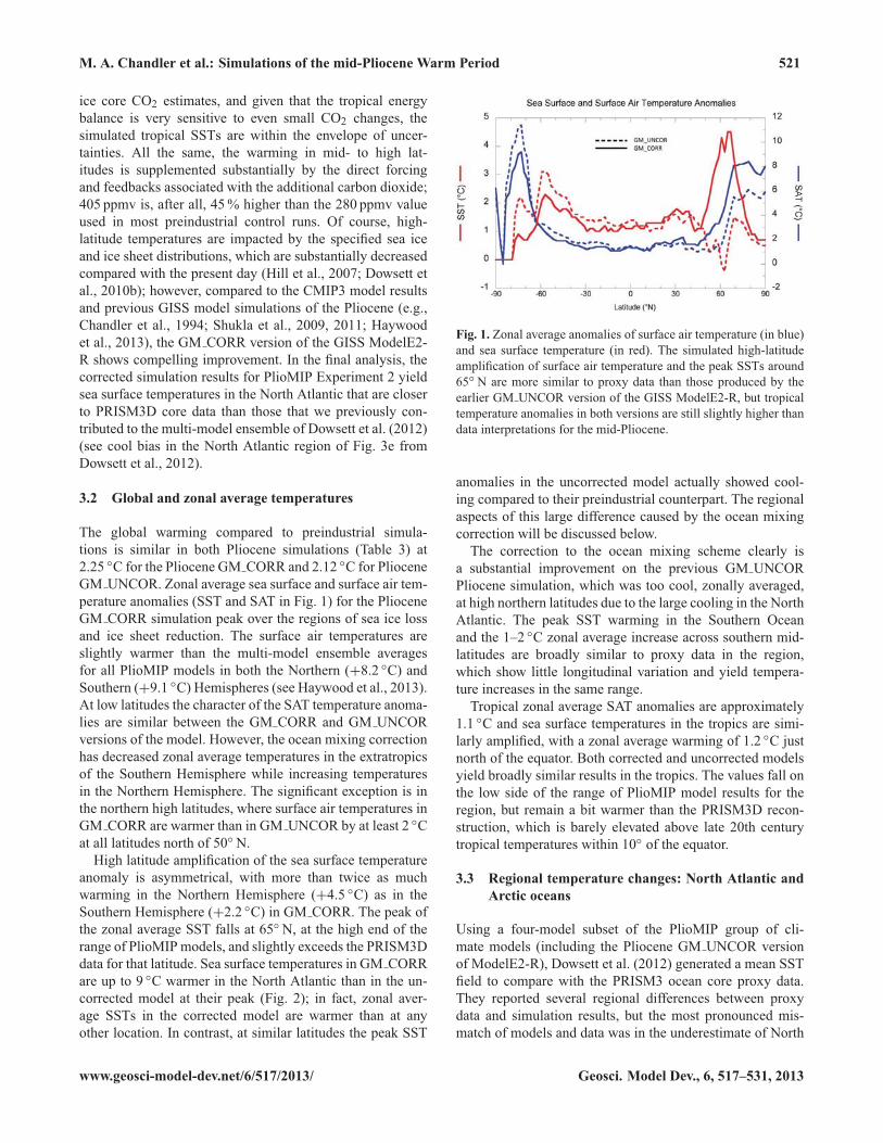
The global warming compared to preindustrial simula-tions is similar in both Pliocene simulations (Table 3) at2.25 ◦C for the Pliocene GM CORR and 2.12 ◦C for PlioceneGM UNCOR. Zonal average sea surface and surface air tem-perature anomalies (SST and SAT in Fig. 1) for the PlioceneGM CORR simulation peak over the regions of sea ice lossand ice sheet reduction. The surface air temperatures areslightly warmer than the multi-model ensemble averagesfor all PlioMIP models in both the Northern (+8.2 ◦C) andSouthern (+9.1 ◦C) Hemispheres (see Haywood et al., 2013).At low latitudes the character of the SAT temperature anoma-lies are similar between the GM CORR and GM UNCORversions of the model. However, the ocean mixing correctionhas decreased zonal average temperatures in the extratropicsof the Southern Hemisphere while increasing temperaturesin the Northern Hemisphere. The significant exception is inthe northern high latitudes, where surface air temperatures inGM CORR are warmer than in GM UNCOR by at least 2 ◦Cat all latitudes north of 50◦ N.High latitude amplification of the sea surface temperature

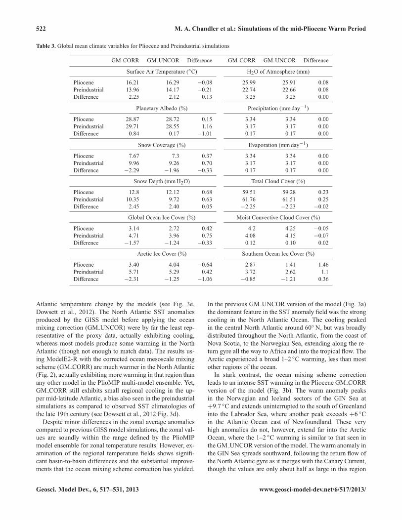
anomaly is asymmetrical, with more than twice as muchwarming in the Northern Hemisphere (+4.5 ◦C) as in theSouthern Hemisphere (+2.2 ◦C) in GM CORR. The peak ofthe zonal average SST falls at 65◦ N, at the high end of therange of PlioMIPmodels, and slightly exceeds the PRISM3Ddata for that latitude. Sea surface temperatures in GM CORRare up to 9 ◦C warmer in the North Atlantic than in the un-corrected model at their peak (Fig. 2); in fact, zonal aver-age SSTs in the corrected model are warmer than at anyother location. In contrast, at similar latitudes the peak SST

Fig. 1. Zonal average anomalies of surface air temperature (in blue)and sea surface temperature (in red). The simulated high-latitudeamplification of surface air temperature and the peak SSTs around65◦ N are more similar to proxy data than those produced by theearlier GM UNCOR version of the GISS ModelE2-R, but tropicaltemperature anomalies in both versions are still slightly higher thandata interpretations for the mid-Pliocene.

anomalies in the uncorrected model actually showed cool-ing compared to their preindustrial counterpart. The regionalaspects of this large difference caused by the ocean mixingcorrection will be discussed below.The correction to the ocean mixing scheme clearly is

a substantial improvement on the previous GM UNCORPliocene simulation, which was too cool, zonally averaged,at high northern latitudes due to the large cooling in the NorthAtlantic. The peak SST warming in the Southern Oceanand the 1–2 ◦C zonal average increase across southern mid-latitudes are broadly similar to proxy data in the region,which show little longitudinal variation and yield tempera-ture increases in the same range.Tropical zonal average SAT anomalies are approximately

1.1 ◦C and sea surface temperatures in the tropics are simi-larly amplified, with a zonal average warming of 1.2 ◦C justnorth of the equator. Both corrected and uncorrected modelsyield broadly similar results in the tropics. The values fall onthe low side of the range of PlioMIP model results for theregion, but remain a bit warmer than the PRISM3D recon-struction, which is barely elevated above late 20th centurytropical temperatures within 10◦ of the equator.

3.3 Regional temperature changes: North Atlantic andArctic oceans

Using a four-model subset of the PlioMIP group of cli-mate models (including the Pliocene GM UNCOR versionof ModelE2-R), Dowsett et al. (2012) generated a mean SSTfield to compare with the PRISM3 ocean core proxy data.They reported several regional differences between proxydata and simulation results, but the most pronounced mis-match of models and data was in the underestimate of North



Table 3. Global mean climate variables for Pliocene and Preindustrial simulations

GM CORR GM UNCOR Difference GM CORR GM UNCOR Difference

Surface Air Temperature (◦C) H2O of Atmosphere (mm)

Pliocene 16.21 16.29 −0.08 25.99 25.91 0.08Preindustrial 13.96 14.17 −0.21 22.74 22.66 0.08Difference 2.25 2.12 0.13 3.25 3.25 0.00

Planetary Albedo (%) Precipitation (mmday−1)Pliocene 28.87 28.72 0.15 3.34 3.34 0.00Preindustrial 29.71 28.55 1.16 3.17 3.17 0.00Difference 0.84 0.17 −1.01 0.17 0.17 0.00

Snow Coverage (%) Evaporation (mmday−1)Pliocene 7.67 7.3 0.37 3.34 3.34 0.00Preindustrial 9.96 9.26 0.70 3.17 3.17 0.00Difference −2.29 −1.96 −0.33 0.17 0.17 0.00

Snow Depth (mmH2O) Total Cloud Cover (%)

Pliocene 12.8 12.12 0.68 59.51 59.28 0.23Preindustrial 10.35 9.72 0.63 61.76 61.51 0.25Difference 2.45 2.40 0.05 −2.25 −2.23 −0.02

Global Ocean Ice Cover (%) Moist Convective Cloud Cover (%)

Pliocene 3.14 2.72 0.42 4.2 4.25 −0.05Preindustrial 4.71 3.96 0.75 4.08 4.15 −0.07Difference −1.57 −1.24 −0.33 0.12 0.10 0.02

Arctic Ice Cover (%) Southern Ocean Ice Cover (%)

Pliocene 3.40 4.04 −0.64 2.87 1.41 1.46Preindustrial 5.71 5.29 0.42 3.72 2.62 1.1Difference −2.31 −1.25 −1.06 −0.85 −1.21 0.36

Atlantic temperature change by the models (see Fig. 3e,Dowsett et al., 2012). The North Atlantic SST anomaliesproduced by the GISS model before applying the oceanmixing correction (GM UNCOR) were by far the least rep-resentative of the proxy data, actually exhibiting cooling,whereas most models produce some warming in the NorthAtlantic (though not enough to match data). The results us-ing ModelE2-R with the corrected ocean mesoscale mixingscheme (GM CORR) are much warmer in the North Atlantic(Fig. 2), actually exhibiting more warming in that region thanany other model in the PlioMIP multi-model ensemble. Yet,GM CORR still exhibits small regional cooling in the up-per mid-latitude Atlantic, a bias also seen in the preindustrialsimulations as compared to observed SST climatologies ofthe late 19th century (see Dowsett et al., 2012 Fig. 3d).Despite minor differences in the zonal average anomalies

compared to previous GISS model simulations, the zonal val-ues are soundly within the range defined by the PlioMIPmodel ensemble for zonal temperature results. However, ex-amination of the regional temperature fields shows signifi-cant basin-to-basin differences and the substantial improve-ments that the ocean mixing scheme correction has yielded.

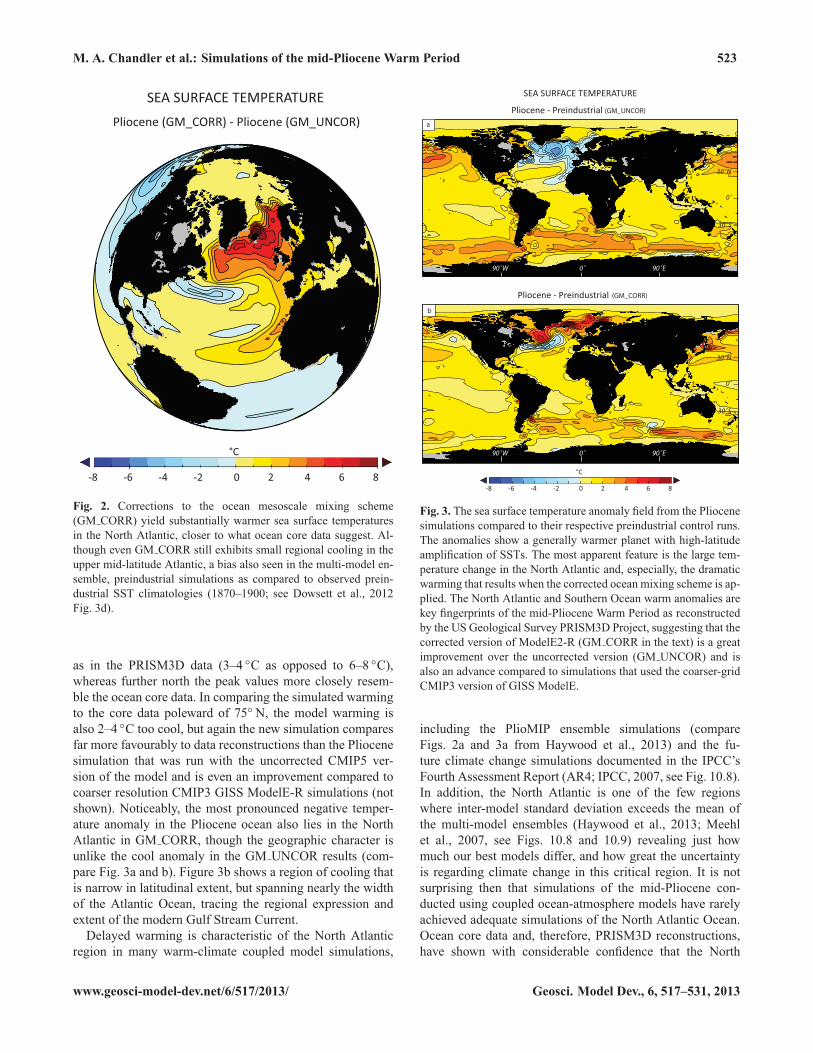
In the previous GM UNCOR version of the model (Fig. 3a)the dominant feature in the SST anomaly field was the strongcooling in the North Atlantic Ocean. The cooling peakedin the central North Atlantic around 60◦ N, but was broadlydistributed throughout the North Atlantic, from the coast ofNova Scotia, to the Norwegian Sea, extending along the re-turn gyre all the way to Africa and into the tropical flow. TheArctic experienced a broad 1–2 ◦C warming, less than mostother regions of the ocean.In stark contrast, the ocean mixing scheme correction

leads to an intense SST warming in the Pliocene GM CORRversion of the model (Fig. 3b). The warm anomaly peaksin the Norwegian and Iceland sectors of the GIN Sea at+9.7 ◦C and extends uninterrupted to the south of Greenlandinto the Labrador Sea, where another peak exceeds +6 ◦Cin the Atlantic Ocean east of Newfoundland. These veryhigh anomalies do not, however, extend far into the ArcticOcean, where the 1–2 ◦C warming is similar to that seen inthe GM UNCOR version of the model. The warm anomaly inthe GIN Sea spreads southward, following the return flow ofthe North Atlantic gyre as it merges with the Canary Current,though the values are only about half as large in this region



-8 -6 -4 -2 0 2 4 6 8

°C

SEA SURFACE TEMPERATUREPliocene (GM_CORR) - Pliocene (GM_UNCOR)

Fig. 2. Corrections to the ocean mesoscale mixing scheme(GM CORR) yield substantially warmer sea surface temperaturesin the North Atlantic, closer to what ocean core data suggest. Al-though even GM CORR still exhibits small regional cooling in theupper mid-latitude Atlantic, a bias also seen in the multi-model en-semble, preindustrial simulations as compared to observed prein-dustrial SST climatologies (1870–1900; see Dowsett et al., 2012Fig. 3d).

as in the PRISM3D data (3–4 ◦C as opposed to 6–8 ◦C),whereas further north the peak values more closely resem-ble the ocean core data. In comparing the simulated warmingto the core data poleward of 75◦ N, the model warming isalso 2–4 ◦C too cool, but again the new simulation comparesfar more favourably to data reconstructions than the Pliocenesimulation that was run with the uncorrected CMIP5 ver-sion of the model and is even an improvement compared tocoarser resolution CMIP3 GISS ModelE-R simulations (notshown). Noticeably, the most pronounced negative temper-ature anomaly in the Pliocene ocean also lies in the NorthAtlantic in GM CORR, though the geographic character isunlike the cool anomaly in the GM UNCOR results (com-pare Fig. 3a and b). Figure 3b shows a region of cooling thatis narrow in latitudinal extent, but spanning nearly the widthof the Atlantic Ocean, tracing the regional expression andextent of the modern Gulf Stream Current.Delayed warming is characteristic of the North Atlantic

region in many warm-climate coupled model simulations,

SEA SURFACE TEMPERATURE

Pliocene - Preindustrial (no GM fix)

Pliocene - Preindustrial (GM fix)

0˚ 90˚E90˚W

0˚

30˚S

0˚ 90˚E90˚W

0˚

30˚N

30˚S

30˚N

(GM_UNCOR)

(GM_CORR)

-8 -6 -4 -2 0 2 4 6 8

°C

a

b

Fig. 3. The sea surface temperature anomaly field from the Pliocenesimulations compared to their respective preindustrial control runs.The anomalies show a generally warmer planet with high-latitudeamplification of SSTs. The most apparent feature is the large tem-perature change in the North Atlantic and, especially, the dramaticwarming that results when the corrected ocean mixing scheme is ap-plied. The North Atlantic and Southern Ocean warm anomalies arekey fingerprints of the mid-Pliocene Warm Period as reconstructedby the US Geological Survey PRISM3D Project, suggesting that thecorrected version of ModelE2-R (GM CORR in the text) is a greatimprovement over the uncorrected version (GM UNCOR) and isalso an advance compared to simulations that used the coarser-gridCMIP3 version of GISS ModelE.

including the PlioMIP ensemble simulations (compareFigs. 2a and 3a from Haywood et al., 2013) and the fu-ture climate change simulations documented in the IPCC’sFourth Assessment Report (AR4; IPCC, 2007, see Fig. 10.8).In addition, the North Atlantic is one of the few regionswhere inter-model standard deviation exceeds the mean ofthe multi-model ensembles (Haywood et al., 2013; Meehlet al., 2007, see Figs. 10.8 and 10.9) revealing just howmuch our best models differ, and how great the uncertaintyis regarding climate change in this critical region. It is notsurprising then that simulations of the mid-Pliocene con-ducted using coupled ocean-atmosphere models have rarelyachieved adequate simulations of the North Atlantic Ocean.Ocean core data and, therefore, PRISM3D reconstructions,have shown with considerable confidence that the North



Atlantic and northward extensions into the GIN Sea expe-rienced strong warming in the Pliocene – greater than any-where else in the global oceans and greater than in other ex-periments in the multi-model PlioMIP ensemble (Haywoodet al., 2013; see Fig. 3). Dowsett et al. (2012) point out thateven accounting for a cool bias in the models compared totheir own preindustrial control simulations, coupled modelsunderestimate North Atlantic warming in the mid-Plioceneby 2–8 ◦C.

3.4 Regional ocean temperature changes: North Pacific,Southern Ocean, and the Tropics

Temperature change throughout the rest of the global oceansis muted by comparison with the North Atlantic and Arctic,but there are still significant anomalies that can be comparedand contrasted to data reconstructions in other key oceanicregions. The North Pacific and Southern Ocean show warm-ing in the Pliocene in both the GM CORR and GM UNCORsimulations (Fig. 3a and b). Unlike the Atlantic anomalies,the sea surface temperatures in the Pacific and SouthernOceans are broad and peak below + 5 ◦C. In addition, thewarming was 2–4 ◦C less once the ocean mixing schemewas corrected. More extreme warm anomalies near the Asianshoreline in the northwest Pacific are supported by oceancore data that Dowsett et al. (2012) give a confidence rat-ing of “Very High”. It is noteworthy that the temperatureanomaly lessens poleward of 45◦ N latitude and into thenortheastern Pacific Ocean in the GM CORR model. Datafrom the Gulf of Alaska do not dispute that trend. Corestaken off the west coast of North America are given a “high-confidence” rating in PRISM project analyses and indicatelevels of Pliocene warming that are not simulated by the cor-rected version of the model.While mid- to high latitude warming is evident in ocean

cores throughout the Southern Ocean there is little longitu-dinal variation in the warming – despite the absence of theWest Antarctic Ice Sheet in the Pliocene boundary condi-tions. ModelE2-R, like the multi-model PlioMIP ensemble,shows that the South Atlantic and southern Indian Oceanregions are somewhat warmer than the corresponding lati-tudes in the South Pacific. This feature tends to be robust,and is also borne out by the PRISM3D reconstructions. Theresults with GM CORR appear to be an improvement com-pared to GM UNCOR, which had broad warming throughoutthe southern high latitudes. However, ocean core data is verylimited at many longitudes in the Southern Ocean and themeridional character of the Pliocene Southern Hemispheresea surface temperatures is not well understood.Tropical temperature change, as mentioned previously, has

proven to be a dilemma for many model-data comparisonsfor past warm periods in Earth history. One of the overar-ching themes from proxy studies of pre-Pleistocene warmclimates is that tropical temperatures have been relativelystable compared to higher latitudes, resulting in decreased

meridional temperature gradients (e.g., Zachos et al., 1994;Galfetti et al., 2007; Pearson et al., 2007; Dowsett et al.,1996, 2010b). In contrast, climate model simulations of thesepast time periods show that when the forcing is either a well-mixed greenhouse gas or the result of changes to solar inso-lation, tropical temperatures respond measurably (e.g., Rindand Chandler, 1991; Chandler et al., 1994; Sloan et al., 1996;Haywood et al., 2000; Jiang et al., 2005).The mid-Pliocene, with its relatively lower levels of at-

mospheric CO2 (compared to earlier warm periods in geo-logic history), has minimal additional forcing in the tropics,thus, tropical SSTs and surface air temperatures warm onlyabout 1 ◦C relative to the preindustrial. Tropical temperatureswarmed another a degree in the Atlantic Ocean when theocean mixing was corrected, but that was related to the factthat the uncorrected model received substantial cool surfaceflow from the unrealistic cold anomaly in the North Atlantic.Otherwise there was little change in response in the tropicsbetween GM CORR and GM UNCORR.Results from the PRISM analyses show that some tropi-

cal regions may in fact have experienced warming on the or-der of 1–2 ◦C, but PRISM also includes a number of siteswhere no temperature increases are discernable. In eachocean basin, the sites that show little or no temperaturechange are in the central or western warm pools, whereasthose sites with minor warming are generally in the eastern-most portions of the basins. All of the ModelE2-R simula-tion results show generally uniform east-west temperature in-creases across all ocean basins and, where minor variationsexist, there is no consistent east-west trend. This permanentEl Nino or “El Padre” character of the tropical SSTs is con-sistent with some Pliocene data and simulations (Shukla etal., 2009 and references therein), but the issue is far fromresolved with both data and modelling studies suggestingENSO variability was still present in the Pliocene (Scroxtonet al., 2011; Watanabe et al., 2011).

3.5 Arctic sea ice

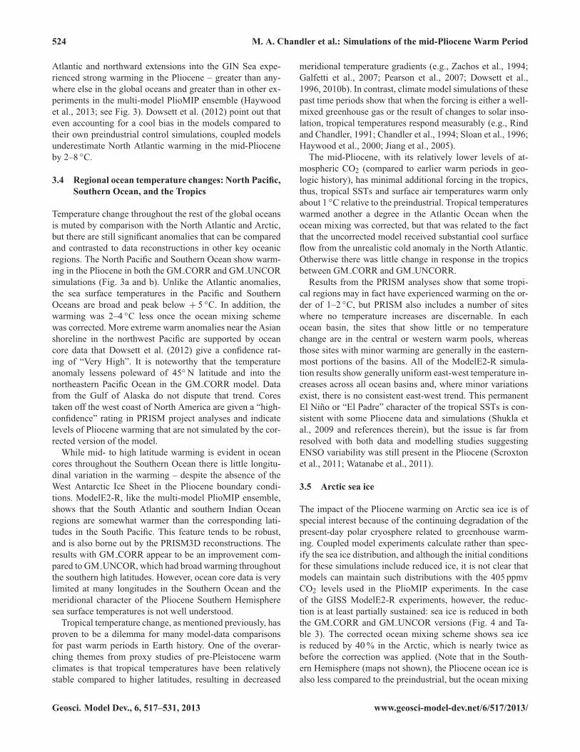
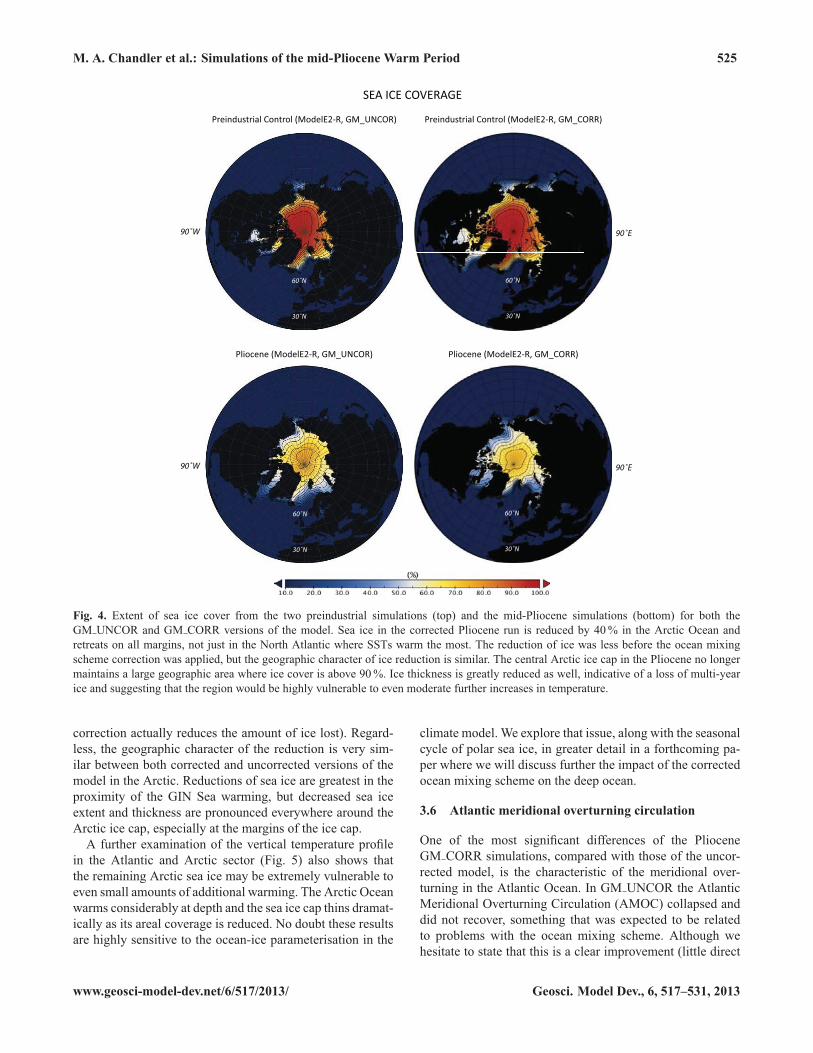
The impact of the Pliocene warming on Arctic sea ice is ofspecial interest because of the continuing degradation of thepresent-day polar cryosphere related to greenhouse warm-ing. Coupled model experiments calculate rather than spec-ify the sea ice distribution, and although the initial conditionsfor these simulations include reduced ice, it is not clear thatmodels can maintain such distributions with the 405 ppmvCO2 levels used in the PlioMIP experiments. In the caseof the GISS ModelE2-R experiments, however, the reduc-tion is at least partially sustained: sea ice is reduced in boththe GM CORR and GM UNCOR versions (Fig. 4 and Ta-ble 3). The corrected ocean mixing scheme shows sea iceis reduced by 40% in the Arctic, which is nearly twice asbefore the correction was applied. (Note that in the South-ern Hemisphere (maps not shown), the Pliocene ocean ice isalso less compared to the preindustrial, but the ocean mixing



SEA ICE COVERAGE

Preindustrial Control (ModelE2-R, GM_UNCOR) Preindustrial Control (ModelE2-R, GM_CORR)

Pliocene (ModelE2-R, GM_UNCOR) Pliocene (ModelE2-R, GM_CORR)

90˚W

90˚W

30˚N

60˚N

30˚N

60˚N

30˚N

60˚N

30˚N

60˚N

90˚E

90˚E

Fig. 4. Extent of sea ice cover from the two preindustrial simulations (top) and the mid-Pliocene simulations (bottom) for both theGM UNCOR and GM CORR versions of the model. Sea ice in the corrected Pliocene run is reduced by 40% in the Arctic Ocean andretreats on all margins, not just in the North Atlantic where SSTs warm the most. The reduction of ice was less before the ocean mixingscheme correction was applied, but the geographic character of ice reduction is similar. The central Arctic ice cap in the Pliocene no longermaintains a large geographic area where ice cover is above 90%. Ice thickness is greatly reduced as well, indicative of a loss of multi-yearice and suggesting that the region would be highly vulnerable to even moderate further increases in temperature.

correction actually reduces the amount of ice lost). Regard-less, the geographic character of the reduction is very sim-ilar between both corrected and uncorrected versions of themodel in the Arctic. Reductions of sea ice are greatest in theproximity of the GIN Sea warming, but decreased sea iceextent and thickness are pronounced everywhere around theArctic ice cap, especially at the margins of the ice cap.A further examination of the vertical temperature profile

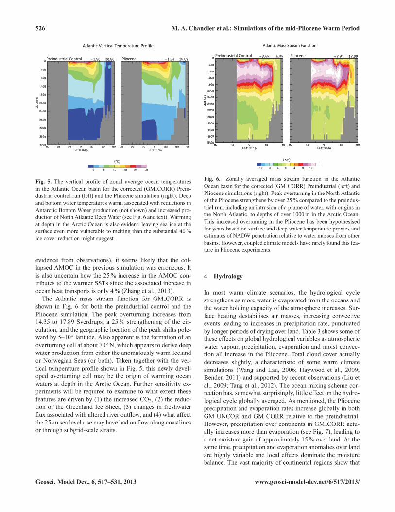
in the Atlantic and Arctic sector (Fig. 5) also shows thatthe remaining Arctic sea ice may be extremely vulnerable toeven small amounts of additional warming. The Arctic Oceanwarms considerably at depth and the sea ice cap thins dramat-ically as its areal coverage is reduced. No doubt these resultsare highly sensitive to the ocean-ice parameterisation in the

climate model. We explore that issue, along with the seasonalcycle of polar sea ice, in greater detail in a forthcoming pa-per where we will discuss further the impact of the correctedocean mixing scheme on the deep ocean.

3.6 Atlantic meridional overturning circulation

One of the most significant differences of the PlioceneGM CORR simulations, compared with those of the uncor-rected model, is the characteristic of the meridional over-turning in the Atlantic Ocean. In GM UNCOR the AtlanticMeridional Overturning Circulation (AMOC) collapsed anddid not recover, something that was expected to be relatedto problems with the ocean mixing scheme. Although wehesitate to state that this is a clear improvement (little direct



Preindustrial Control Pliocene

Fig. 5. The vertical profile of zonal average ocean temperaturesin the Atlantic Ocean basin for the corrected (GM CORR) Prein-dustrial control run (left) and the Pliocene simulation (right). Deepand bottom water temperatures warm, associated with reductions inAntarctic Bottom Water production (not shown) and increased pro-duction of North Atlantic DeepWater (see Fig. 6 and text). Warmingat depth in the Arctic Ocean is also evident, leaving sea ice at thesurface even more vulnerable to melting than the substantial 40%ice cover reduction might suggest.

evidence from observations), it seems likely that the col-lapsed AMOC in the previous simulation was erroneous. Itis also uncertain how the 25% increase in the AMOC con-tributes to the warmer SSTs since the associated increase inocean heat transports is only 4% (Zhang et al., 2013).The Atlantic mass stream function for GM CORR is

shown in Fig. 6 for both the preindustrial control and thePliocene simulation. The peak overturning increases from14.35 to 17.89 Sverdrups, a 25% strengthening of the cir-culation, and the geographic location of the peak shifts pole-ward by 5–10◦ latitude. Also apparent is the formation of anoverturning cell at about 70◦ N, which appears to derive deepwater production from either the anomalously warm Icelandor Norwegian Seas (or both). Taken together with the ver-tical temperature profile shown in Fig. 5, this newly devel-oped overturning cell may be the origin of warming oceanwaters at depth in the Arctic Ocean. Further sensitivity ex-periments will be required to examine to what extent thesefeatures are driven by (1) the increased CO2, (2) the reduc-tion of the Greenland Ice Sheet, (3) changes in freshwaterflux associated with altered river outflow, and (4) what affectthe 25-m sea level rise may have had on flow along coastlinesor through subgrid-scale straits.

Preindustrial Control Pliocene

Atlantic Mass Stream Function

Fig. 6. Zonally averaged mass stream function in the AtlanticOcean basin for the corrected (GM CORR) Preindustrial (left) andPliocene simulations (right). Peak overturning in the North Atlanticof the Pliocene strengthens by over 25% compared to the preindus-trial run, including an intrusion of a plume of water, with origins inthe North Atlantic, to depths of over 1000m in the Arctic Ocean.This increased overturning in the Pliocene has been hypothesisedfor years based on surface and deep water temperature proxies andestimates of NADW penetration relative to water masses from otherbasins. However, coupled climate models have rarely found this fea-ture in Pliocene experiments.

4 Hydrology

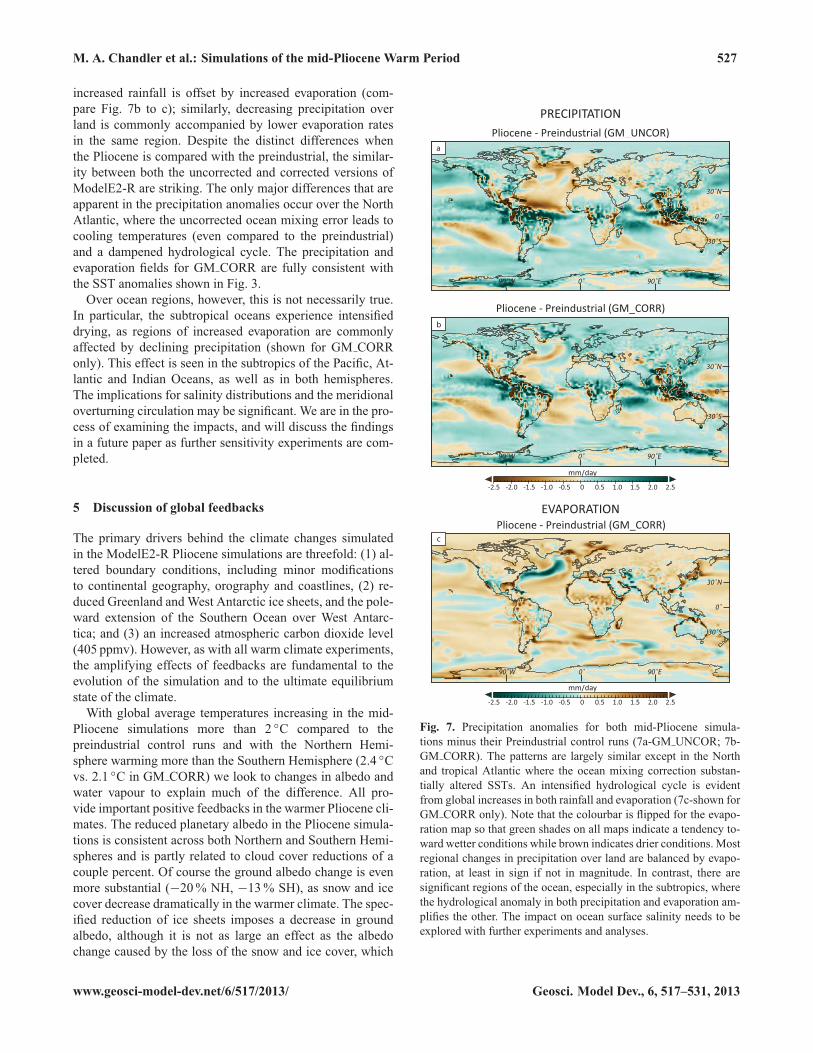
In most warm climate scenarios, the hydrological cyclestrengthens as more water is evaporated from the oceans andthe water holding capacity of the atmosphere increases. Sur-face heating destabilises air masses, increasing convectiveevents leading to increases in precipitation rate, punctuatedby longer periods of drying over land. Table 3 shows some ofthese effects on global hydrological variables as atmosphericwater vapour, precipitation, evaporation and moist convec-tion all increase in the Pliocene. Total cloud cover actuallydecreases slightly, a characteristic of some warm climatesimulations (Wang and Lau, 2006; Haywood et al., 2009;Bender, 2011) and supported by recent observations (Liu etal., 2009; Tang et al., 2012). The ocean mixing scheme cor-rection has, somewhat surprisingly, little effect on the hydro-logical cycle globally averaged. As mentioned, the Plioceneprecipitation and evaporation rates increase globally in bothGM UNCOR and GM CORR relative to the preindustrial.However, precipitation over continents in GM CORR actu-ally increases more than evaporation (see Fig. 7), leading toa net moisture gain of approximately 15% over land. At thesame time, precipitation and evaporation anomalies over landare highly variable and local effects dominate the moisturebalance. The vast majority of continental regions show that



increased rainfall is offset by increased evaporation (com-pare Fig. 7b to c); similarly, decreasing precipitation overland is commonly accompanied by lower evaporation ratesin the same region. Despite the distinct differences whenthe Pliocene is compared with the preindustrial, the similar-ity between both the uncorrected and corrected versions ofModelE2-R are striking. The only major differences that areapparent in the precipitation anomalies occur over the NorthAtlantic, where the uncorrected ocean mixing error leads tocooling temperatures (even compared to the preindustrial)and a dampened hydrological cycle. The precipitation andevaporation fields for GM CORR are fully consistent withthe SST anomalies shown in Fig. 3.Over ocean regions, however, this is not necessarily true.

In particular, the subtropical oceans experience intensifieddrying, as regions of increased evaporation are commonlyaffected by declining precipitation (shown for GM CORRonly). This effect is seen in the subtropics of the Pacific, At-lantic and Indian Oceans, as well as in both hemispheres.The implications for salinity distributions and the meridionaloverturning circulation may be significant. We are in the pro-cess of examining the impacts, and will discuss the findingsin a future paper as further sensitivity experiments are com-pleted.

5 Discussion of global feedbacks

The primary drivers behind the climate changes simulatedin the ModelE2-R Pliocene simulations are threefold: (1) al-tered boundary conditions, including minor modificationsto continental geography, orography and coastlines, (2) re-duced Greenland andWest Antarctic ice sheets, and the pole-ward extension of the Southern Ocean over West Antarc-tica; and (3) an increased atmospheric carbon dioxide level(405 ppmv). However, as with all warm climate experiments,the amplifying effects of feedbacks are fundamental to theevolution of the simulation and to the ultimate equilibriumstate of the climate.With global average temperatures increasing in the mid-

Pliocene simulations more than 2 ◦C compared to thepreindustrial control runs and with the Northern Hemi-sphere warming more than the Southern Hemisphere (2.4 ◦Cvs. 2.1 ◦C in GM CORR) we look to changes in albedo andwater vapour to explain much of the difference. All pro-vide important positive feedbacks in the warmer Pliocene cli-mates. The reduced planetary albedo in the Pliocene simula-tions is consistent across both Northern and Southern Hemi-spheres and is partly related to cloud cover reductions of acouple percent. Of course the ground albedo change is evenmore substantial (−20% NH, −13% SH), as snow and icecover decrease dramatically in the warmer climate. The spec-ified reduction of ice sheets imposes a decrease in groundalbedo, although it is not as large an effect as the albedochange caused by the loss of the snow and ice cover, which

PRECIPITATIONPliocene - Preindustrial (GM_UNCOR)

Pliocene - Preindustrial (GM_CORR)

-2.5 0.5 1.5 2.5-0.5 0.20.1-5.1-0.2- 1.00

mm/day

EVAPORATION

-2.5 0.5 1.5 2.5-0.5 0.20.1-5.1-0.2- 1.00

mm/day

Pliocene - Preindustrial (GM_CORR)

0˚ 90˚E90˚W

0˚

30˚S

30˚N

0˚ 90˚E90˚W

0˚

30˚S

30˚N

0˚ 90˚E90˚W

0˚

30˚S

30˚N

a

c

b

Fig. 7. Precipitation anomalies for both mid-Pliocene simula-tions minus their Preindustrial control runs (7a-GM UNCOR; 7b-GM CORR). The patterns are largely similar except in the Northand tropical Atlantic where the ocean mixing correction substan-tially altered SSTs. An intensified hydrological cycle is evidentfrom global increases in both rainfall and evaporation (7c-shown forGM CORR only). Note that the colourbar is flipped for the evapo-ration map so that green shades on all maps indicate a tendency to-ward wetter conditions while brown indicates drier conditions. Mostregional changes in precipitation over land are balanced by evapo-ration, at least in sign if not in magnitude. In contrast, there aresignificant regions of the ocean, especially in the subtropics, wherethe hydrological anomaly in both precipitation and evaporation am-plifies the other. The impact on ocean surface salinity needs to beexplored with further experiments and analyses.



is calculated by the GCM. Snow depth, while decreasing inthe Northern Hemisphere, actually increases on average inthe Southern Hemisphere in the Pliocene simulations. Thisless obvious result is due to the great reduction in circum-Antarctic sea ice, which leads to increased evaporation acrosswarm waters and large increases in snow accumulation overthe margins of East Antarctica. Although the West Antarc-tica Ice Sheet has been removed, and West Antarctica it-self is mostly submerged, sea ice formation across that highlatitude ocean still forms a platform that allows snow accu-mulation for much of the year. This begs the question as towhether or not the GISS ModelE2-R would actually supportthe re-initiation or maintenance of continental glaciation onany portion of West Antarctica.As mentioned above, the other factor in planetary albedo

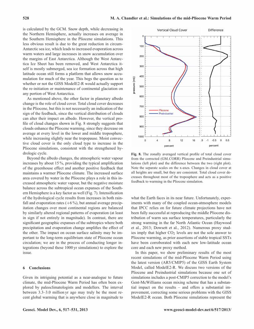
change is the role of cloud cover. Total cloud cover decreasesin the Pliocene, but this is not necessarily an indication of thesign of the feedback, since the vertical distribution of cloudscan alter their impact on albedo. However, the vertical pro-file of cloud changes shown in Fig. 8 strongly suggests thatclouds enhance the Pliocene warming, since they decrease onaverage at every level in the lower and middle troposphere,while increasing slightly near the tropopause. Moist convec-tive cloud cover is the only cloud type to increase in thePliocene simulations, consistent with the strengthened hy-drologic cycle.Beyond the albedo changes, the atmospheric water vapour

increases by about 15%, providing the typical amplificationof the greenhouse effect and another positive feedback thatmaintains a warmer Pliocene climate. The increased surfacearea covered by water in the Pliocene plays a role in this in-creased atmospheric water vapour, but the negative moisturebalance across the subtropical ocean expanses of the South-ern Hemisphere is a key factor as well (Fig. 7). Intensificationof the hydrological cycle results from increases in both rain-fall and evaporation rates (+6%), but annual average precip-itation changes over most continental regions are balancedby similarly altered regional patterns of evaporation (at leastin sign if not entirely in magnitude). In contrast, there aresignificant geographic expanses of the subtropics where bothprecipitation and evaporation change amplifies the effect ofthe other. The impact on ocean surface salinity may be im-portant to the long-term equilibrium state of Pliocene oceancirculation; we are in the process of conducting longer in-tegrations (beyond these 1000 yr simulations) to explore theissue.

6 Conclusions

Given its intriguing potential as a near-analogue to futureclimate, the mid-Pliocene Warm Period has often been ex-plored by paleoclimatologists and modellers. The intervalbetween 3.3–3.0 million yr ago may truly be the most re-cent global warming that is anywhere close in magnitude to

Fig. 8. The zonally averaged vertical profile of total cloud coverfrom the corrected (GM CORR) Pliocene and Preindustrial simu-lations (left plot) and the difference between the two (right plot).Note the separate scales on the x-axes. Changes in cloud cover atall heights are small, but they are consistent. Total cloud cover de-creases throughout most of the troposphere and acts as a positivefeedback to warming in the Pliocene simulation.

what the Earth faces in its near future. Unfortunately, exper-iments with many of the coupled ocean-atmosphere modelsthat IPCC relies on for future climate projections have notbeen fully successful at reproducing the middle Pliocene dis-tribution of warm sea surface temperatures, particularly thestrong warming in the far North Atlantic Ocean (Haywoodet al., 2013; Dowsett et al., 2012). Numerous proxy stud-ies imply that higher CO2 levels are not the sole answer toPliocene warming, as prior assertions of stable tropical SSTshave been corroborated with each new low-latitude oceancore and each new proxy method.In this paper, we show preliminary results of the most

recent simulations of the mid-Pliocene Warm Period usingthe latest version (AR5/CMIP5) of the GISS Earth SystemModel, called ModelE2-R. We discuss two versions of thePliocene and Preindustrial simulations because one set ofsimulations includes a post-CMIP5 correction to the model’sGent-McWilliams ocean mixing scheme that has a substan-tial impact on the results – and offers a substantial im-provement, correcting some serious problems with the GISSModelE2-R ocean. Both Pliocene simulations represent the



NASA/GISS contribution to the Pliocene Model Intercom-parison Project (PlioMIP, Experiment 2) and are used inPhase 1 of the PlioMIP multi-model ensemble studies. Go-ing forward, we will adopt only the model version that in-corporates the corrected mixing scheme (GM CORR in thispaper). Many of our results from the Pliocene GM CORRsimulation fall squarely within the range defined by othercoupled models in the PlioMIP ensemble, but we empha-sise here some features that would be outliers in the en-semble ranges. The most prominent is the simulation of alarge region of warming in the North Atlantic and Greenland-Iceland-Norwegian Sea (large areas covered by SST anoma-lies greater than + 4◦C, with distinct peaks of more than9 ◦C). This is by far the most accurate portrayal of this keygeographic region by any version of the NASA/GISS fam-ily of models to date and comparisons with the PlioceneGM UNCOR simulations shows that the ocean mixingscheme correction is the key factor in the improved results– at least for ModelE2-R. There are still model-data differ-ences to be addressed, and these preliminary results requirefurther analysis in order to fully understand the physical pro-cesses involved in the warming of the North Atlantic and inthe changes to ocean circulation. However, we believe thatcontinued development of key physical routines in the GISSatmospheric model, along with higher resolution and recentcorrections made to the Gent-McWilliams mixing parame-terisation in the Russell ocean model, have led to an EarthSystem Model that will produce more accurate projectionsof both past and future climate.

Acknowledgements. The authors acknowledge the support of theNASA High-End Computing (NEC) Program through the NASACenter for Climate Simulation (NCCS) at Goddard Space FlightCenter; MAC acknowledges the National Science Foundation Pa-leoclimate Program Grant No. ATM-0214400; HJD acknowledgesthe support of the US Geological Survey Climate and Land UseChange R&D Program; HJD and MAC thank the U.S.G.S. PowellCenter for Analysis and Synthesis for supporting the PlioMIPinitiative.

Edited by: J. C. Hargreaves

References

Bender, F. A. M.: Planetary albedo in a strongly forced climate, assimulated by the CMIP3 models, Theor. Appl. Climatol., 105,529–535, doi:10.1007/s00704-011-0411-2, 2011.

Chandler, M. A. and Rind, D.: The Influence of Warm NorthAtlantic Sea Surface Temperatures on the Pliocene Climate:GCM Sensitivity Experiments, EOS, Transactions, AmericanGeophysical Union, 73(14) Supp., 169, 1992.

Chandler, M. A., Rind, D., and Thompson, R. S.: Joint investi-gations of the middle Pliocene climate II: GISS GCM North-ern Hemisphere results, Global Planet. Change, 9, 197–219,doi:10.1016/0921-8181(94)90016-7, 1994.

Conkright, M. E., Levitus, S., O’Brien, T., Boyer, T. P., Stephens,C., Johnson, D., Stathoplos, L., Baranova, O., Antonov, J.,Gelfeld, R., Burney, J., Rochester, J., and Forgy, C.: World OceanDatabase 1998 Documentation and Quality Control, NationalOceanographic Data Center, Silver Spring, MD, 1998.

Del Genio, A. D., Yao, M.-S., Kovari, W., and Lo, K. K.-W.: A prognostic cloud water parameterisation for globalclimate models, J. Climate, 9, 270–304, doi:10.1175/1520-0442(1996)009<0270:APCWPF>2.0.CO;2, 1996.

Dowsett, H. J., Barron, J., and Poore, R.: Middle Pliocene sea sur-face temperatures: A global reconstruction, Marine Micropale-ontol., 27, 13–25, 1996.

Dowsett, H. J., Robinson, M. M., and Foley, K. M.: Pliocene three-dimensional global ocean temperature reconstruction, Clim. Past,5, 769–783, doi:10.5194/cp-5-769-2009, 2009.

Dowsett, H., Robinson, M., Haywood, A., Salzmann, U., Hill, D.,Sohl, L., Chandler, M., Williams, M., Foley, K., and Stoll, D.:The PRISM3D paleoenvironmental reconstruction, Stratigraphy,7, 123–139, 2010a.

Dowsett, H. J., Robinson, M. M., Stoll, D. K., and Foley, K. M.:Mid-Piacenzian mean annual sea surface temperature analysisfor data-model comparisons, Stratigraphy, 7, 189–198, 2010b.

Galfetti, T., Bucher, H., Brayard, A., Hochuli, P. A., Weissert, H.,Guodun, K., Atudorei, V., and Guex, J.: Late Early Triassic cli-mate change: Insights from carbonate carbon isotopes, sedimen-tary evolution and ammonoid palaeobiogeography, Palaeogeogr.Palaeoclimatol, 243, 394–411, 2007.

Gent, P. R. and McWilliams, J. C.: Isopycnal mixing in ocean cir-culation models, J. Phys. Oceanogr., 20, 150–155, 1990.

Gent, P. R., Willebrand, J., McDougall, T. J., and McWilliams, J. C.:Parameterizing eddy-induced tracer transports in ocean circula-tion models, J. Phys. Oceanogr., 25, 463–474, 1995.

Hansen, J. E. and Sato, Mki.: Paleoclimate implications for human-made climate change, in Climate Change: Inferences fromPaleoclimate and Regional Aspects, edited by: Berger, A.,Mesinger, F., and Sijacki, D., Springer, Vienna, Austria, 21–48,doi:10.1007/978-3-7091-0973-1 2, 2012.

Hansen, J. E., Ruedy, R., Lacis, A., Sato, Mki., Nazarenko, L.,Tausnev, N., Tegen, I., and Koch, D.: Climate modelling in theglobal warming debate. In General Circulation Model Develop-ment, edited by: Randall, D., Academic Press, 127–164, 2000.

Hansen, J. E., Sato, Mki., Nazarenko, L., Ruedy, R., Lacis, A.,Koch, D., Tegen, I., Hall, T., Shindell, D., Santer, B., Stone, P.,Novakov, T., Thomason, L., Wang, R., Wang, Y., Jacob, D., Hol-landsworth, S., Bishop, L., Logan, J., Thompson, A., Stolarski,R., Lean, J., Willson, R., Levitus, S., Antonov, J., Rayner, N.,Parker, D., and Christy, J.: Climate forcings in Goddard Insti-tute for Space Studies SI2000 simulations, J. Geophys. Res., 107,4347, doi:10.1029/2001JD001143, 2002.

Haywood, A. M., Valdes, P. J., and Sellwood, B. W.: Global scalepaleoclimate reconstruction of the middle Pliocene climate usingthe UKMOGCM: initial results, Global Planet. Chang., 25, 239–256, 2000.

Haywood, A.M., Chandler, M. A., Valdes, P. J., Salzmann, U., Lunt,D. J., and Dowsett, H. J.: Comparison of mid-Pliocene climatepredictions produced by the HadAM3 and GCMAM3 GeneralCirculation Models, Global Planet. Chang., 66, 208–224, 2009.

Haywood, A.M., Dowsett, H. J., Otto-Bliesner, B., Chandler, M. A.,Dolan, A. M., Hill, D. J., Lunt, D. J., Robinson, M. M., Rosen-



bloom, N., Salzmann, U., and Sohl, L. E.: Pliocene Model Inter-comparison Project (PlioMIP): experimental design and bound-ary conditions (Experiment 1), Geosci. Model Dev., 3, 227–242,doi:10.5194/gmd-3-227-2010, 2010.

Haywood, A. M., Dowsett, H. J., Robinson, M. M., Stoll, D. K.,Dolan, A. M., Lunt, D. J., Otto-Bliesner, B., and Chandler, M.A.: Pliocene Model Intercomparison Project (PlioMIP): experi-mental design and boundary conditions (Experiment 2), Geosci.Model Dev., 4, 571–577, doi:10.5194/gmd-4-571-2011, 2011.

Haywood, A. M., Hill, D. J., Dolan, A. M., Otto-Bliesner, B. L.,Bragg, F., Chan, W.-L., Chandler, M. A., Contoux, C., Dowsett,H. J., Jost, A., Kamae, Y., Lohmann, G., Lunt, D. J., Abe-Ouchi,A., Pickering, S. J., Ramstein, G., Rosenbloom, N. A., Salz-mann, U., Sohl, L., Stepanek, C., Ueda, H., Yan, Q., and Zhang,Z.: Large-scale features of Pliocene climate: results from thePliocene Model Intercomparison Project, Clim. Past, 9, 191–209,doi:10.5194/cp-9-191-2013, 2013.

Hill, D. J., Haywood, A. M., Hindmarsh, R. C. M., and Valdes, P.J.: Characterising ice sheets during the Pliocene: evidence fromdata and models, in: Deep-time perspectives on climate change:marrying the signal from computer models and biological prox-ies, edited by: Williams, M., Haywood, A. M., Gregory, J., andSchmidt, D., Micropalaeontol. Soc., Spec. Pub. Geol. Soc., Lon-don, 517–538, 2007.

IPCC: Climate Change 2007: The Physical Science Basis. Con-tribution of Working Group I to the Fourth Assessment Reportof the Intergovernmental Panel on Climate Change, edited by:Solomon, S., Qin, D., Manning, M., Chen, Z., Marquis, M., Av-eryt, K. B., Tignor, M., and Miller, H. L., Cambridge Univ. Press,Cambridge, UK, and New York, 996 pp., 2007.

Jiang, D. B., Wang, H. J., Ding, Z. L., Lang, X. M., and Drange,H.: Modeling the middle Pliocene climate with a global atmo-spheric general circulation model, J. Geophys. Res.-Atmos., 110,D14107, doi:10.1029/2004JD005639, 2005.

Kurschner, W. M., Van der Burgh, J., Visscher, H., and Dilcher, D.L.: Oak leaves as biosensors of late Neogene and early Pleis-tocene paleoatmospheric CO2 concentrations, Mar. Micropale-ontol., 27, 299–312, 1996.

Liu, Y. H., Key, J. R., and Wang, X. J.: Influence of changesin sea ice concentration and cloud cover on recent Arcticsurface temperature trends, Geophys. Res. Lett., 36, L20710,doi:10.1029/2009GL040708, 2009.

Lythe, M. B., Vaughn, D. G., and the BEDMAP Consortium:BEDMAP – bed topography of the Antarctic, Cambridge, UK,British Antarctic Survey, 2000, Digital media available at: http://nsidc.org/data/atlas/, last access: 23 January 2011.

Matthews, E.: Global vegetation and land use: New high-resolution data bases for climate studies, J. Clim.Appl. Meteorol., 22, 474–487, doi:10.1175/1520-0450(1983)022<0474:GVALUN>2.0.CO;2, 1983.

Matthews, E.: Prescription of Land-Surface Boundary Conditionsin GISS GCM II: A Simple Method Based on High-ResolutionVegetation Data Bases, NASA TM-86096, National Aeronauticsand Space Administration, 1984.

Meehl, G. A., Stocker, T. F., Collins, W. D., Friedlingstein, P., Gaye,A. T., Gregory, J. M., Kitoh, A., Knutti, R., Murphy, J. M., Noda,A., Raper, S. C. B., Watterson, I. G., Weaver, A. J., and Zhao,Z.-C.: Global Climate Projections, in: Climate Change 2007:The Physical Science Basis, Contribution of Working Group I

to the Fourth Assessment Report of the Intergovernmental Panelon Climate Change, edited by: Solomon, S., Qin, D., Manning,M., Chen, Z., Marquis, M., Averyt, K. B., Tignor, M., and Miller,H. L., Cambridge University Press, Cambridge, United Kingdomand New York, NY, USA, 2007.

Pagani, M., Liu, Z. H., LaRiviere, J., and Ravelo, A. C.: HighEarth-system climate sensitivity determined from Pliocenecarbon dioxide concentrations, Nat. Geosci., 3, 27–30,doi:10.1038/NGEO724, 2010.

Pearson, P. N., van Dongen, B. E., Nicholas, C. J., Pancost, R. D.,Schouten, S., Singano, J. M., and Wade, B. S.: Stable warm trop-ical climate through the Eocene Epoch, Geology, 35, 211–214,2007.

Pollard, D. and DeConto, R. M.: ModellingWest Antarctic ice sheetgrowth and collapse through the past five million years, Nature,458, 329–332, 2009.

Poore, R. Z. and Chandler, M. A.: Simulating past climates, Thedata-model connection, Global Planet. Change, 9, 165–167,1994.

Raymo, M. E., Grant, B., Horowitz, M., and Rau, G. H.:Mid-Pliocene warmth: Stronger greenhouse and stronger con-veyor, Mar. Micropaleontol., 27, 313–326, doi:10.1016/0377-8398(95)00048-8, 1996.

Redi, M. H.: Oceanic isopycnal mixing by coordinate rotation, J.Phys. Oceanogr., 12, 1154–1158, 1982.

Rind, D. and Chandler, M. A.: Increased ocean heat trans-ports and warmer climate, J. Geophys. Res., 96, 7437–7461,doi:10.1029/91JD00009, 1991.

Russell, G. L., Miller, J. R., and Rind, D.: A coupled atmosphere-ocean model for transient climate change studies, Atmos.-Ocean,33, 683–730, 1995.

Salzmann, U., Haywood, A.M., Lunt D. J., Valdes, P. J., and Hill, D.J.: A new Global Biome Reconstruction and Data-Model Com-parison for the middle Pliocene, Global Ecol. Biogeogr., 17, 432–447, 2008.

Schmidt, G. A., Ruedy, R., Hansen, J. E., Aleinov, I., Bell, N.,Bauer, M., Bauer, S., Cairns, B., Canuto, V., Cheng, Y., Del Ge-nio, A., Faluvegi, G., Friend, A. D., Hall, T. M., Hu, Y., Kelley,M., Kiang, N. Y., Koch, D., Lacis, A. A., Lerner, J., Lo, K. K.,Miller, R. L., Nazarenko, L., Oinas, V., Perlwitz, J. P., Perlwitz,Ju., Rind, D., Romanou, A., Russell, G. L., Sato, Mki., Shindell,D. T., Stone, P. H., Sun, S., Tausnev, N., Thresher, D., and Yao,M.-S.: Present day atmospheric simulations using GISSModelE:Comparison to in-situ, satellite and reanalysis data, J. Climate,19, 153–192, doi:10.1175/JCLI3612.1, 2006.

Schmidt, G. A., Kelley, M., Nazarenko, L., Ruedy, R., Russell, G.L., Aleinov, I., Bauer, M., Bauer, S., Bhat, M. K., Bleck, R.,Canuto, V., Chen, Y., Ye Cheng, Clune, T. L., Del Genio, A., deFainchtein, R., Faluvegi, G., Hansen, J. E., Healy, R. J., Kiang,N. Y., Koch, D., Lacis, A. A., LeGrande, A. N., Lerner, J., Lo,K. K., Marshall, J., Menon, S., Miller, R. L., Oinas, V., Oloso, A.O., Perlwitz, J., Puma, M. J., Putman,W.M., Rind, D., Romanou,A., Sato, M., Shindell, D. T., Shan Sun, Syed, R. A., Tausnev, N.,Tsigaridis, K., Unger, N., Voulgarakis, A., Mao-Sung Yao, andJinlun Zhang: Configuration and assessment of the GISS Mod-elE2 contributions to the CMIP5 archive, in preparation, 2013.

Scroxton, N., Bonham, S. G., Rickaby, R. E. M., Lawrence, S. H. F.,Hermoso, M., and Haywood, A. M.: Persistent El Nino–SouthernOscillation variation during the Pliocene Epoch, Paleoceanogra-



phy, 26, PA2215, doi:10.1029/2010PA002097, 2011.Seki, O., Foster, G. L., Schmidt, D. N., Mackensen, A., Kawamura,K., and Pancost, R. D.: Alkenone and boron-based PliocenepCO2 records, Earth Planet. Sci. Lett., 292, 201–211, 2010.

Shukla, S. P., Chandler, M. A., Jonas, J., Sohl, L. E., Mankoff, K.,and Dowsett, H.: Impact of a permanent El Nino (El Padre) andIndian Ocean Dipole in warm Pliocene climates, Paleoceanogra-phy, 24, PA2221, doi:10.1029/2008PA001682, 2009.

Shukla, S. P., Chandler, M. A., Rind, D., Sohl, L. E., Jonas, J., andLerner, J.: Teleconnections in a warmer climate: The Plioceneperspective, Clim. Dynam., 37, 1869–1887, doi:10.1007/s00382-010-0976-y, 2011.

Sloan, L. C., Crowley, T. C., and Pollard, D.: Modeling of middlePliocene climate with the NCAR GENESIS general circulationmodel, Mar. Micropaleontol., 27, 51–61, 1996.

Sohl, L. E., Chandler, M. A., Schmunk, R. B., Mankoff, K., Jonas, J.A., Foley, K. M., and Dowsett, H. J.: PRISM3/GISS topographicreconstruction, U. S. Geol. Surv. Data Series, 419, 6 pp., 2009.

Tang, Q. H., Leng, G. Y., and Groisman, P. Y.: European hot sum-mers associated with a reduction of cloudiness, J. Climate, 25,3637–3644, doi:10.1175/JCLI-D-12-00040.1, 2012.

Visbeck, M., Marshall, J., Haine, T., and Spall, M.: Specification ofEddy Transfer Coefficients in Coarse-Resolution Ocean Circula-tionModels, J. Phys. Oceanogr., 27, 381–402, doi:10.1175/1520-0485(1997)027<0381:SOETCI>2.0.CO;2, 1997.

Wang, H. L. and Lau, K. M.: Atmospheric hydrological cycle in thetropics in twentieth century coupled climate simulations, Int. J.Climatol., 26, 655–678, 2006.

Watanabe, T., Suzuki, A., Minobe, S., Kawashima, T., Kameo, K.,Minoshima, K., Aguilar, Y. M., Wani, R., Kawahata, H., Sowa,K., Nagai, T., and Kase, T.: Permanent El Nino during Pliocenewarm period not suppoted by coral evidence, Nature, 471, 209–211, doi:10.1038/nature09777, 2011.

Zachos, J. M., Scott, L. D., and Lohmann, K. C.: Evolution of earlyCenozoic marine temperatures, Paleoceanography, 9, 353–387,1994.

Zhang, Z.-S., Nisancioglu, K. H., Chandler, M. A., Haywood, A.M., Otto-Bliesner, B. L., Ramstein, G., Stepanek, C., Abe-Ouchi,A., Chan, W.-L., Bragg, F. J., Contoux, C., Dolan, A. M., Hill, D.J., Jost, A., Kamae, Y., Lohmann, G., Lunt, D. J., Rosenbloom,N. A., Sohl, L. E., and Ueda, H.: Mid-pliocene Atlantic merid-ional overturning circulation not unlike modern?, Clim. Past Dis-cuss., 9, 1297–1319, doi:10.5194/cpd-9-1297-2013, 2013.


Documents

Simulations of the mid-Pliocene Warm Period using two ... · Bab al-Mandab Connects Red Sea and Gulf of Aden 140 25000 parameterised parameterised Malacca Between Malay Peninsula