Computers & Operations Research 39 (2012) 659–663

Contents lists available at ScienceDirect

Computers & Operations Research

0305-05

doi:10.1

� Corr

E-m

wangjib

journal homepage: www.elsevier.com/locate/caor

Single-machine makespan minimization scheduling with nonlinearshortening processing times

Ming-Zheng Wang a,�, Ji-Bo Wang b

a School of Management Science and Engineering, Dalian University of Technology, Dalian 116024, Chinab School of Science, Shenyang Aerospace University, Shenyang 110136, China

a r t i c l e i n f o

Available online 10 May 2011

Keywords:

Scheduling

Single-machine

Makespan

Nonlinear shortening processing times

48/$ - see front matter & 2011 Elsevier Ltd. A

016/j.cor.2011.05.001

esponding author.

ail addresses: mzhwang@dlut.edu.cn (M.-Z. W

o75@yahoo.com.cn (J.-B. Wang).

a b s t r a c t

In this paper, we consider the single-machine makespan minimization scheduling problem with

nonlinear shortening processing times. By the nonlinear shortening processing times, we mean that the

processing times of jobs are non-increasing nonlinear functions of their starting times. The computa-

tional complexity of the general problem remains an open problem, but we show that even with the

introduction of nonlinear shortening processing times to job processing times, some special cases

remain polynomially solvable. We also show that an optimal schedule of the general makespan

minimization problem is V-shaped with respect to job normal processing times. A heuristic algorithm

which utilize the V-shaped property is proposed, and computational experiments show that it is

effective and efficient in obtaining near-optimal solutions.

& 2011 Elsevier Ltd. All rights reserved.

1. Introduction

Traditional scheduling problems usually involve jobs withconstant, independent processing times. In practice, however,we often encounter settings in which the job processing timesincrease or decrease over time. Applications of these models canbe found, among others, in fire fighting, emergency medicine,police, machine maintenance, computer science, and radarscience. Researchers have formulated this phenomenon intodifferent models and solved different problems for various cri-teria. For example, consider the production of custom industrialsteel products such as vault doors or boiler covers, whereby rawiron is first converted into a batch of iron ingots in an electricfurnace. The ingots are then sequentially processed on a machineinto different products. An ingot has to reach a thresholdtemperature before it can be processed by the machine into aproduct. The longer an ingot waits for processing (i.e., the later itis processed by the machine), the cooler it becomes. After waitingfor a period of time, an ingot needs to be reheated to thethreshold temperature before the machine can work on it.Consequently, extra time is required to produce each productfrom an ingot that has waited longer than a certain time interval(Barketau et al. [3]). On the other hand, an example consideringthe so-called ‘‘learning effect’’ can be described by a non-increas-ing start time dependent function. Assume that a worker has toassemble a large number of similar products. The time required

ll rights reserved.

ang),

by the worker to assemble one product depends on his knowl-edge, skills, organization of his working place and others. Theworker learns how to produce. After some time, he is betterskilled, his working place is better organized and his knowledgehas increased. As a result of his learning, the time required toassemble one product decreases. Another example is the processby which aerial threats are to be recognized by a radar station. Inthis case, a radar station has detected some objects approachingit. The time required to recognize the objects decreases as theobjects get closer. Thus, the later the objects are detected, the lesstime needed for their recognition (Wang and Xia [13]). Extensivesurveys of scheduling models and problems concerning start timedependent job processing times can be found in Alidaee andWomer [2], Cheng et al. [4] and Gawiejnowicz [5]. More recentpapers which have considered scheduling jobs with time dependentprocessing include Barketau et al. [3], Ng et al. [9], Li et al. [10],Oron [11], Toksari and Guner [12], Yang [14], Yang et al. [15], andZhao and Tang [16].

According to the notion mentioned above, many schedulingproblems with linear, piecewise linear or nonlinear time depen-dent processing times are studied in the literature. There aremany interesting efficient ordering policies provided for somescheduling problems with linear or piecewise linear processingtimes. However, there are less efficient rules available for thosewith nonlinear processing times. Only a few heuristic algorithmswere proposed. For example, Gupta and Gupta [7] studied thesingle-machine makespan scheduling problem with nonlinearprocessing times. In this study, the complexity of the problemwas conjectured to be NP-hard. Thus, Gupta and Gupta [7]proposed two heuristic algorithms to solve the problem. Further,Alidaee [1] proposed a more efficient heuristic algorithm to solve

J.-B. Wang, J.-J. Wang / Computers & Operations Research 39 (2012) 659–663660

the problem proposed by Gupta and Gupta [7] when the poly-nomial function is differentiable.

In this paper, we focus on a more general nonlinear shorteningprocessing times model. This model is adopted from Wang andXia [13]. The paper is organized as follows: In Section 2, weformulate the model. In Section 3, we consider the makespanminimization problem. In Section 4, we propose a heuristicalgorithm utilized the V-shaped property for the makespanminimization problem followed by computational experiments,where the definition of the V-shaped property is as follows:A schedule is V-shaped with respect to job normal processingtimes (aj) if jobs are arranged in descending order if they areplaced before the job with the smallest aj but in ascending order ifplaced after it. In Section 5, we consider some special cases whichcan be solved in polynomial time. The last section is the summaryand future research.

2. Problem formulation

Given a single machine and a set J¼ fJ1,J2, . . . ,Jng of n indepen-dent and non-preemptive jobs, our goal is to find a sequence thatminimizes makespan. All jobs are available for processing at time 0.The machine can handle one job at a time and preemption is notallowed. Associated with each job Jjðj¼ 1,2, . . . ,nÞ there is a normalprocessing time aj. Let pjðtÞ be the actual processing time of job Jj

if it is started at time t in a sequence. Gupta and Gupta [7]considered the model in which pjðtÞ ¼ aj0þaj1tþ � � � þajmtm, whereaj0,aj1, . . . ,ajm are non-negative constants. Wang and Xia [13]considered the model in which pjðtÞ ¼ ajð1�utÞ, where uZ0,uðPn

j ¼ 1 aj�aminÞo1 and amin ¼mini ¼ 1,2,...,nai (the conditionsensure that all job processing times are positive in a feasibleschedule). In this paper, we consider a single-machine schedulingwith nonlinear processing times which is adopted from Wang andXia [13]. Specially, we consider a general nonlinear processingtimes model as follows:

pjðtÞ ¼ ajð1�utÞa, ð1Þ

where uZ0 is a given parameter and aZ0 is a given constantrepresenting a rate of change, which is common for all jobs. It isassumed that the normal processing times satisfy the followingconditions: uZ0, uð

Pnj ¼ 1 aj�aminÞo1 and amin ¼mini ¼ 1,2,...,nai

(The conditions ensure that all job processing times are positivein a feasible schedule). Obviously, if a¼ 1 the model (1) is themodel of Wang and Xia [13].

For a given schedule p¼ ½J1,J2, . . . ,Jn�, CjðpÞ represents thecompletion time of job Jj. Let CmaxðpÞ ¼maxfCjjj¼ 1,2, . . . ,ngrepresent the makespan of a given permutation p. In the remain-ing part of the paper, all the problems considered will be denotedusing the three-field notation schema ajbjg introduced by Gra-ham et al. [6], where a indicates the scheduling environment, bdescribes the job characteristics or restrictive requirements, and gdefines the objective function to be minimized.

3. Makespan minimization problem

In this section, we will consider the single-machine schedulingmakespan minimization problem with nonlinear shortening pro-cessing times. In the classical single-machine makespan pro-blems, the makespan value is sequence-independent. In theproblem 1jpjðtÞ ¼ ajð1�utÞjCmax, the makespan value is alsosequence-independent (Wang and Xia [13]). However, the pro-blem 1jpjðtÞ ¼ ajð1�utÞajCmax cannot always be solved optimallyby sequencing jobs in non-decreasing order of aj (the SPT rule) or

by sequencing jobs in non-increasing order of aj (the LPT rule), theexample is as follows:

Counter-example 1: n¼ 3,a1 ¼ 1,a2 ¼ 2,a3 ¼ 15, u¼ 0:1,a¼ 2.The SPT sequence is p1 ¼ ½J1,J2,J3�, Cmaxðp1Þ ¼ 1þ2�ð1�0:1�1Þ2

þ15�ð1�0:1�ð1þ2�ð1�0:1�1Þ2ÞÞ2 ¼ 10:7897. The LPT sequence isp2 ¼ ½J3,J2,J1�, Cmaxðp2Þ ¼ 15þ2�ð1�0:1�15Þ2þ1�ð1�0:1�ð15þ2�ð1�0:1�15Þ2ÞÞ2 ¼ 15:8025. Obviously, the optimal sequence isp3 ¼ ½J2,J1,J3�, Cmaxðp3Þ ¼ 2þ1�ð1�0:1�2Þ2þ15�ð1�0:1�ð2þ1�ð1�0:1�2Þ2ÞÞ2 ¼ 10:7654.

From counter-example 1, if a40 and aa1, we know that theclassical SPT rule or LPT rule cannot always give an optimalsolution for the makespan minimization problem. It remains anopen problem, we conjecture that the problem 1jpjðtÞ ¼

ajð1�utÞa,a40,aa1jCmax is NP-hard. Now, we prove that theoptimal schedule of problem 1jpjðtÞ ¼ ajð1�utÞa, a40, aa1jCmax

is V-shaped with respect to the job normal processing times(SPT and LPT rules provide optimal solutions to special cases ofthe problem in which the optimal solution has a specificV-shape).

Theorem 1. For the problem 1jpjðtÞ ¼ ajð1�utÞa,a40,aa1jCmax,an optimal schedule exists which is V-shaped with respect to the job

normal processing times.

Proof. Consider a schedule p with three consecutive jobs, Ji,Jj and Jk,i.e., p¼ ½S1,Ji,Jj,Jk,S2� such that aj4ai and aj4ak, where S1 and S2

denote partial schedules. We show that an interchange between Ji

and Jj or between Jj and Jk reduces the value of total completiontime. Let p1 be the schedule obtained from p by interchanging Ji andJj, i.e., p1 ¼ ½S1,Jj,Ji,Jk,S2�. Similarly, let p2 be the schedule obtainedfrom p by interchanging Jj and Jk, i.e., p2 ¼ ½S1,Ji,Jk,Jj,S2�. Further-more, let t denote the completion time of the last job in S1. Then, thecontribution of the three jobs to the total completion time is

DðpÞ ¼ tþaið1�utÞaþajð1�uðtþaið1�utÞaÞÞa

þakð1�uðtþaið1�utÞaþajð1�uðtþaið1�utÞaÞÞaÞÞa

¼ tþaið1�utÞaþajð1�ut�uaið1�utÞaÞa

þakð1�ut�uaið1�utÞa�uajð1�ut�uaið1�utÞaÞaÞa: ð2Þ

Similar expressions are easily obtained for p1 and p2:

Dðp1Þ ¼ tþajð1�utÞaþaið1�ut�uajð1�utÞaÞa

þakð1�ut�uajð1�utÞa�uaið1�ut�uajð1�utÞaÞaÞa, ð3Þ

Dðp2Þ ¼ tþaið1�utÞaþakð1�ut�uaið1�utÞaÞa

þajð1�ut�uaið1�utÞa�uakð1�ut�uaið1�utÞaÞaÞa: ð4Þ

It follows that

DðpÞ�Dðp1Þ ¼ ðai�ajÞð1�utÞaþajð1�ut�uaið1�utÞaÞa

�aið1�ut�uajð1�utÞaÞaþak½ð1�ut�uaið1�utÞa

�uajð1�ut�uaið1�utÞaÞaÞa�ð1�ut�uajð1�utÞa

�uaið1�ut�uajð1�utÞaÞaÞa�, ð5Þ

DðpÞ�Dðp2Þ ¼ ðaj�akÞð1�ut�uaið1�utÞaÞa

þakð1�ut�uaið1�utÞa�uajð1�ut�uaið1�utÞaÞaÞa

�ajð1�ut�uaið1�utÞa�uakð1�ut�uaið1�utÞaÞaÞa: ð6Þ

Let l¼ aj=ai, x¼ uaið1�utÞa�1, then from (5), we have

DðpÞ�Dðp1Þ

ð1�utÞaai¼ 1�lþlð1�xÞa�ð1�lxÞa

þak

ð1�utÞaai½ð1�ut�uaið1�utÞa�uajð1�ut�uaið1�utÞaÞaÞa

�ð1�ut�uajð1�utÞa�uaið1�ut�uajð1�utÞaÞaÞa�: ð7Þ

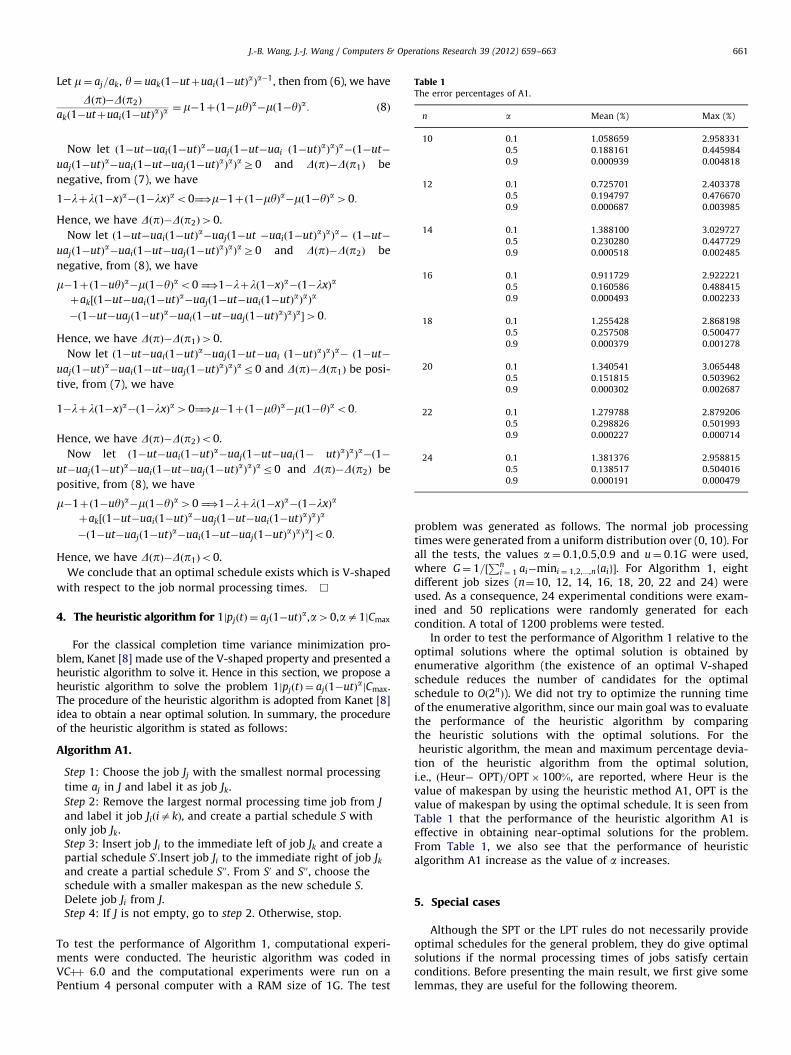
Table 1The error percentages of A1.

n a Mean (%) Max (%)

10 0.1 1.058659 2.958331

0.5 0.188161 0.445984

0.9 0.000939 0.004818

12 0.1 0.725701 2.403378

0.5 0.194797 0.476670

0.9 0.000687 0.003985

14 0.1 1.388100 3.029727

0.5 0.230280 0.447729

0.9 0.000518 0.002485

16 0.1 0.911729 2.922221

0.5 0.160586 0.488415

0.9 0.000493 0.002233

18 0.1 1.255428 2.868198

0.5 0.257508 0.500477

0.9 0.000379 0.001278

20 0.1 1.340541 3.065448

0.5 0.151815 0.503962

0.9 0.000302 0.002687

22 0.1 1.279788 2.879206

0.5 0.298826 0.501993

0.9 0.000227 0.000714

24 0.1 1.381376 2.958815

0.5 0.138517 0.504016

0.9 0.000191 0.000479

J.-B. Wang, J.-J. Wang / Computers & Operations Research 39 (2012) 659–663 661

Let m¼ aj=ak, y¼ uakð1�utþuaið1�utÞaÞa�1, then from (6), we have

DðpÞ�Dðp2Þ

akð1�utþuaið1�utÞaÞa¼ m�1þð1�myÞa�mð1�yÞa: ð8Þ

Now let ð1�ut�uaið1�utÞa�uajð1�ut�uai ð1�utÞaÞaÞa�ð1�ut�

uajð1�utÞa�uaið1�ut�uajð1�utÞaÞaÞaZ0 and DðpÞ�Dðp1Þ be

negative, from (7), we have

1�lþlð1�xÞa�ð1�lxÞao0¼)m�1þð1�myÞa�mð1�yÞa40:

Hence, we have DðpÞ�Dðp2Þ40.

Now let ð1�ut�uaið1�utÞa�uajð1�ut �uaið1�utÞaÞaÞa� ð1�ut�

uajð1�utÞa�uaið1�ut�uajð1�utÞaÞaÞaZ0 and DðpÞ�Dðp2Þ be

negative, from (8), we have

m�1þð1�uyÞa�mð1�yÞao0 ¼)1�lþlð1�xÞa�ð1�lxÞa

þak½ð1�ut�uaið1�utÞa�uajð1�ut�uaið1�utÞaÞaÞa

�ð1�ut�uajð1�utÞa�uaið1�ut�uajð1�utÞaÞaÞa�40:

Hence, we have DðpÞ�Dðp1Þ40.

Now let ð1�ut�uaið1�utÞa�uajð1�ut�uai ð1�utÞaÞaÞa� ð1�ut�

uajð1�utÞa�uaið1�ut�uajð1�utÞaÞaÞar0 and DðpÞ�Dðp1Þ be posi-

tive, from (7), we have

1�lþlð1�xÞa�ð1�lxÞa40¼)m�1þð1�myÞa�mð1�yÞao0:

Hence, we have DðpÞ�Dðp2Þo0.

Now let ð1�ut�uaið1�utÞa�uajð1�ut�uaið1� utÞaÞaÞa�ð1�

ut�uajð1�utÞa�uaið1�ut�uajð1�utÞaÞaÞar0 and DðpÞ�Dðp2Þ be

positive, from (8), we have

m�1þð1�uyÞa�mð1�yÞa40 ¼)1�lþlð1�xÞa�ð1�lxÞa

þak½ð1�ut�uaið1�utÞa�uajð1�ut�uaið1�utÞaÞaÞa

�ð1�ut�uajð1�utÞa�uaið1�ut�uajð1�utÞaÞaÞa�o0:

Hence, we have DðpÞ�Dðp1Þo0.

We conclude that an optimal schedule exists which is V-shaped

with respect to the job normal processing times. &

4. The heuristic algorithm for 1jpjðtÞ ¼ ajð1�utÞa,a40,aa1jCmax

For the classical completion time variance minimization pro-blem, Kanet [8] made use of the V-shaped property and presented aheuristic algorithm to solve it. Hence in this section, we propose aheuristic algorithm to solve the problem 1jpjðtÞ ¼ ajð1�utÞajCmax.The procedure of the heuristic algorithm is adopted from Kanet [8]idea to obtain a near optimal solution. In summary, the procedureof the heuristic algorithm is stated as follows:

Algorithm A1.

Step 1: Choose the job Jj with the smallest normal processing

time aj in J and label it as job Jk.

Step 2: Remove the largest normal processing time job from J

and label it job JiðiakÞ, and create a partial schedule S withonly job Jk.Step 3: Insert job Ji to the immediate left of job Jk and create apartial schedule S0.Insert job Ji to the immediate right of job Jk

and create a partial schedule S00. From S0 and S00, choose theschedule with a smaller makespan as the new schedule S.Delete job Ji from J.Step 4: If J is not empty, go to step 2. Otherwise, stop.

To test the performance of Algorithm 1, computational experi-ments were conducted. The heuristic algorithm was coded inVCþþ 6.0 and the computational experiments were run on aPentium 4 personal computer with a RAM size of 1G. The test

problem was generated as follows. The normal job processingtimes were generated from a uniform distribution over (0, 10). Forall the tests, the values a¼ 0:1,0:5,0:9 and u¼ 0:1G were used,where G¼ 1=½

Pni ¼ 1 ai�mini ¼ 1,2,...,nfaig�. For Algorithm 1, eight

different job sizes (n¼10, 12, 14, 16, 18, 20, 22 and 24) wereused. As a consequence, 24 experimental conditions were exam-ined and 50 replications were randomly generated for eachcondition. A total of 1200 problems were tested.

In order to test the performance of Algorithm 1 relative to theoptimal solutions where the optimal solution is obtained byenumerative algorithm (the existence of an optimal V-shapedschedule reduces the number of candidates for the optimalschedule to Oð2n

Þ). We did not try to optimize the running timeof the enumerative algorithm, since our main goal was to evaluatethe performance of the heuristic algorithm by comparingthe heuristic solutions with the optimal solutions. For theheuristic algorithm, the mean and maximum percentage devia-

tion of the heuristic algorithm from the optimal solution,i.e., ðHeur� OPTÞ=OPT� 100%, are reported, where Heur is thevalue of makespan by using the heuristic method A1, OPT is thevalue of makespan by using the optimal schedule. It is seen fromTable 1 that the performance of the heuristic algorithm A1 iseffective in obtaining near-optimal solutions for the problem.From Table 1, we also see that the performance of heuristicalgorithm A1 increase as the value of a increases.

5. Special cases

Although the SPT or the LPT rules do not necessarily provideoptimal schedules for the general problem, they do give optimalsolutions if the normal processing times of jobs satisfy certainconditions. Before presenting the main result, we first give somelemmas, they are useful for the following theorem.

J.-B. Wang, J.-J. Wang / Computers & Operations Research 39 (2012) 659–663662

Lemma 1. atð1�tÞa�1�1þð1�tÞar0 if aZ1 and 0rtr1.

Proof. Let hðtÞ ¼ atð1�tÞa�1�1þð1�tÞa. By taking the first deri-

vative of hðtÞ with respect to t, we have h0ðtÞ ¼�aða�1Þtð1�tÞa�2r0 for aZ1 and 0rtr1. Hence, hðtÞ is decreasing on0rtr1, and we have hðtÞrhð0Þ ¼ 0. &

Lemma 2. ð1�ð1�ltÞaÞ�lð1�ð1�tÞaÞr0 if lZ1, aZ1, 0rtr1and 0rltr1.

Proof. Let f ðlÞ ¼ ð1�ð1�ltÞaÞ�lð1�ð1�tÞaÞ. Then we have

f 0ðlÞ ¼ atð1�ltÞa�1�1þð1�tÞa

and

f 00ðlÞ ¼ �aða�1Þt2ð1�ltÞa�2r0:

Hence, f 0ðlÞ is decreasing on lZ1, aZ1, 0rtr1 and 0rltr1for f 00ðlÞr0. In addition, from Lemma 1, we have

f 0ð1Þ ¼ atð1�tÞa�1�1þð1�tÞar0:

Therefore, f 0ðlÞr f 0ð1Þr0 for lZ1, aZ1, 0rtr1 and 0rltr1.

Hence, f ðlÞ is decreasing on lZ1, aZ1, 0rtr1 and 0rltr1.

Also, f ðlÞr f ð1Þ ¼ 0 for lZ1, aZ1, 0rtr1 and 0rltr1. &

Lemma 3. ð1�ð1�ltÞaÞ�lð1�ð1�tÞaÞZ0 if lZ1, 0rar1,0rtr1 and 0rltr1.

Proof. Similar to the proof of Lemma 2. &

Lemma 4. ð1�x�yÞa�ð1�xÞaZ�ay if 0rxr1, 0ryr1, xþyr1and aZ1.

Proof. Let f ðzÞ ¼ za ðz40Þ. Then we have f 0ðzÞ ¼ aza�1 andf 00ðzÞ ¼ aða�1Þza�2

Z0. Hence, f 0ðzÞ is increasing on z40 andaZ1 for f 00ðzÞZ0. According to the mean value theorem, for anyz40 and z040, there exists a point z between z and z0, such thatf ðzÞ�f ðz0Þ ¼ f 0ðzÞðz�z0Þ: Let z¼ 1�x�y and z0 ¼ 1�x. Then we haveð1�x�yÞa�ð1�xÞa ¼�ayðzÞa�1

Z�ayð1�xÞa�1Z�ay: &

Lemma 5. ð1�x�yÞa�ð1�xÞar�ay if 0rxr1, 0ryr1, xþyr1and 0rar1.

Proof. Similar to the proof of Lemma 4. &

Theorem 2. For the problem 1jpjðtÞ ¼ ajð1�utÞajCmax,

(i)

if ajr1=ua and aZ1, then an optimal schedule can be obtained

by sequencing the jobs in non-decreasing order of aj (the SPT rule);

(ii) if ajr1=ua and 0rar1, then an optimal schedule can be

obtained by sequencing the jobs in non-increasing order of aj

(the LPT rule).

Proof. Let p and p0 be two job schedules where the differencebetween p and p0 is a pairwise interchange of two adjacent jobs Jj

and Jk, that is, p¼ ½S1,Jj,Jk,S2�,p0 ¼ ½S1,Jk,Jj,S2�, where S1 and S2 arepartial sequences. To further simplify the notation, let t denotethe completion time of the last job in S1 and Jh be the first jobin S2. To show p dominates p0, it suffices to show thatCkðpÞrCjðp0Þ and CnðpÞrCnðp0Þ for any Jn in S2. Under p, thecompletion times of jobs Jj and Jk are

CjðpÞ ¼ tþajð1�utÞa

and

CkðpÞ ¼ tþajð1�utÞaþakð1�uðtþajð1�utÞaÞÞa: ð9Þ

Under p0, the completion times of jobs Jk and Jj are

Ckðp0Þ ¼ tþakð1�utÞa

and

Cjðp0Þ ¼ tþakð1�utÞaþajð1�uðtþakð1�utÞaÞÞa: ð10Þ

Based on Eqs. (9) and (10), we have

Cjðp0Þ�CkðpÞ ¼ ðak�ajÞð1�utÞaþajð1�ut�uakð1�utÞaÞa

�akð1�ut�uajð1�utÞaÞa: ð11Þ

(i) Suppose ajrak.

By substituting x¼ uajð1�utÞa�1 and l¼ ak=aj, into Eq. (4), we

have

Cjðp0Þ�CkðpÞð1�utÞaaj

¼ lð1�ð1�xÞaÞ�ð1�ð1�lxÞaÞ:

From Lemma 2, we have Cjðp0Þ�CkðpÞZ0.

Note that

Chðp0Þ ¼ Cjðp0Þþahð1�uCjðp0ÞÞa ð12Þ

and

ChðpÞ ¼ CkðpÞþahð1�uCkðpÞÞa: ð13Þ

Taking the difference between Eqs. (12) and (13), we have

Chðp0Þ�ChðpÞ¼ Cjðp0Þ�CkðpÞþah½ð1�uCjðp0ÞÞa�ð1�uCkðpÞÞa�¼ Cjðp0Þ�CkðpÞþah½ð1�uCkðpÞ�uCjðp0ÞþuCkðpÞÞa�ð1�uCkðpÞÞa�

ZCjðp0Þ�CkðpÞ�uaahðCjðp0Þ�CkðpÞÞ ðfrom Lemma 4Þ

¼ ðCjðp0Þ�CkðpÞÞð1�uaahÞZ0 due to ajr1

ua

� �:

Thus Chðp0ÞZChðpÞ. In other word, we have showed that the first

job Jh in S2, which starts earlier in p than p0, completes earlier in

p. Similarly, we have Cnðp0ÞZCnðpÞ for any Jn in S2. This completes

the proof.

(ii) If ajr1=ua and 0rar1, then from the case (i), Lemmas 3

and 5, the result can be easily obtained. &

6. Summary and future research

In this paper we have studied the single-machine schedulingproblem with nonlinear shortening processing times. We showedthat the makespan minimization problem can be optimally solvedunder certain conditions. However, the optimal job sequence ofthe makespan minimization problem is still unknown if aj41=ua,a40 and aa1, but we proved that the optimal sequence has aV-shaped property with respect to the normal processing times. Itis clearly worthwhile for future research to investigate this openproblem, consider the nonlinear shortening processing times inthe context of other scheduling problems, for example, flow shopscheduling problem, study other objective functions, or proposemore sophisticated and efficient heuristics.

Acknowledgments

We are grateful to an anonymous referee for his/her helpfulcomments on an earlier version of this paper. This research waspartially supported by a research grant from the Program ofNational Natural Science Foundation of China (Nos. 11001181 and71031002), the National Natural Science Foundation of China forDistinguished Young Scholars (Grant No. 70725004).

References

[1] Alidaee B. A heuristic solution procedure to minimize makespan on a singlemachine with non-linear cost functions. Journal of the Operational ResearchSociety 1990;41:1065–8.

J.-B. Wang, J.-J. Wang / Computers & Operations Research 39 (2012) 659–663 663

[2] Alidaee B, Womer NK. Scheduling with time dependent processing times:review and extensions. Journal of the Operational Research Society1999;50:711–20.

[3] Barketau MS, Cheng TCE, Ng CT, Kotov V, Kovalyov MY. Batch scheduling ofstep deteriorating jobs. Journal of Scheduling 2008;11:17–28.

[4] Cheng TCE, Ding Q, Lin BMT. A concise survey of scheduling with time-dependent processing times. European Journal of Operational Research2004;152:1–13.

[5] Gawiejnowicz S. Time-dependent scheduling. Berlin: Springer; 2008.[6] Graham RL, Lawler EL, Lenstra JK, Rinnooy Kan AHG. Optimization and

approximation in deterministic sequencing and scheduling: a survey. Annalsof Discrete Mathematics 1979;5:287–326.

[7] Gupta JND, Gupta SK. Single facility scheduling with nonlinear processingtimes. Computers and Industrial Engineering 1998;14:387–93.

[8] Kanet JJ. Minimizing variation of flow time in single machine systems.Management Science 1981;27:1453–9.

[9] Ng CT, Wang J-B, Cheng TCE, Liu LL. A branch-and-bound algorithm forsolving a two-machine flow shop problem with deteriorating jobs. Compu-ters and Operations Research 2010;37:83–90.

[10] Li Y, Li G, Sun L, Xu Z. Single machine scheduling of deteriorating jobs tominimize total absolute differences in completion times. InternationalJournal of Production Economics 2009;118:424–9.

[11] Oron D. Single machine scheduling with simple linear deterioration tominimize total absolute deviation of completion times. Computers andOperations Research 2008;35:2071–8.

[12] Toksari MD, Guner E. The common due-date early/tardy scheduling problemon a parallel machine under the effects of time-dependent learning and

linear and nonlinear deterioration. Expert Systems with Applications2010;37:92–112.

[13] Wang J-B, Xia Z-Q. Scheduling jobs under decreasing linear deterioration.Information Processing Letters 2005;94:63–9.

[14] Yang S-J. Single-machine scheduling problems with both start-time depen-

dent learning and position dependent aging effects under deterioratingmaintenance consideration. Applied Mathematics and Computation 2011;

217:3321–9.[15] Yang S-J, Yang D-L, Cheng TCE. Single-machine due-window assignment and

scheduling with job-dependent aging effects and deteriorating maintenance.Computers and Operations Research 2010;37:1510–4.

[16] Zhao C, Tang C. A note to due-window assignment and single machinescheduling with deteriorating jobs and a rate-modifying activity, Computersand Operations Research 2010, doi:10.1016/j.cor.2010.04.006.