Single machine scheduling with controllable release and processing parameters

Discrete Applied Mathematics 154 (2006) 2178–2199www.elsevier.com/locate/dam

Single machine scheduling with controllable release and processingparameters

Natalia V. Shakhlevicha, Vitaly A. Strusevichb

aSchool of Computing, University of Leeds, Leeds LS2 9JT, UKbSchool of Computing and Mathematical Sciences, University of Greenwich, Old Royal Naval College, Park Row, London SE10 9LS, UK

Received 24 December 2002; received in revised form 17 September 2004; accepted 21 April 2005Available online 23 March 2006

Abstract

This paper considers single machine scheduling problems in which the job processing times and/or their release dates arecontrollable. Possible changes to the controllable parameters are either individual or done by controlling the relevant processing orrelease rate. The objective is to minimize the sum of the makespan plus the cost for changing the parameters. For the problems ofthis type, we provide a number of polynomial-time algorithms and give a fairly complete complexity classification.© 2006 Elsevier B.V. All rights reserved.

MSC: Primary 90B35; secondary 90B30;90B06

Keywords: Single machine scheduling; Controllable processing times; Controllable processing speeds; Controllable release dates; Controllablerelease speeds

1. Introduction

We consider a series of single machine scheduling problems that may serve as mathematical models that arise insupply chain scheduling. Various aspects of supply chain scheduling have been systematically studied by Hall and hiscoauthors, see [1,4,8,9]. These papers address the issues of coordination and cooperation between the elements of thesupply chain and analyze operational decisions taken in deterministic machine environment (an assembly model, amanufacturer with several suppliers, etc.).

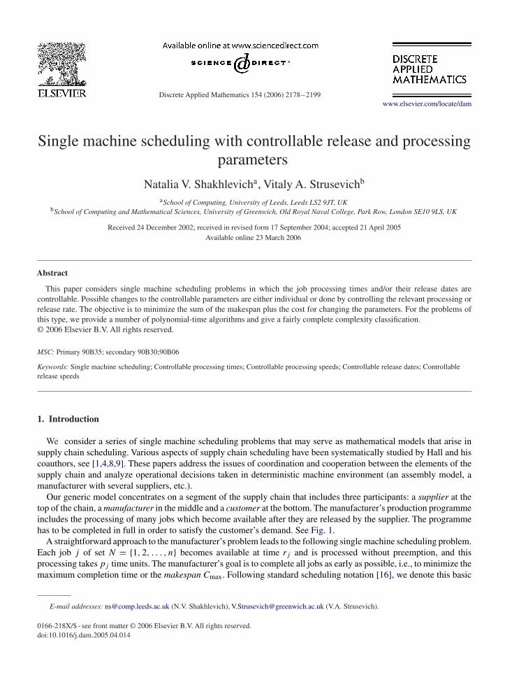
Our generic model concentrates on a segment of the supply chain that includes three participants: a supplier at thetop of the chain, a manufacturer in the middle and a customer at the bottom. The manufacturer’s production programmeincludes the processing of many jobs which become available after they are released by the supplier. The programmehas to be completed in full in order to satisfy the customer’s demand. See Fig. 1.

A straightforward approach to the manufacturer’s problem leads to the following single machine scheduling problem.Each job j of set N = {1, 2, . . . , n} becomes available at time rj and is processed without preemption, and thisprocessing takes pj time units. The manufacturer’s goal is to complete all jobs as early as possible, i.e., to minimize themaximum completion time or the makespan Cmax. Following standard scheduling notation [16], we denote this basic

E-mail addresses: [email protected] (N.V. Shakhlevich), [email protected] (V.A. Strusevich).

0166-218X/$ - see front matter © 2006 Elsevier B.V. All rights reserved.doi:10.1016/j.dam.2005.04.014

http://www.elsevier.com/locate/dam

mailto:[email protected]

mailto:[email protected]

N.V. Shakhlevich, V.A. Strusevich / Discrete Applied Mathematics 154 (2006) 2178–2199 2179

Fig. 1. Supply chain and controllable parameters.

problem by 1|rj |Cmax. Let the jobs be numbered in non-decreasing order of their release dates, i.e.,

r1 �r2 � · · · �rn. (1)

It is well-known that an optimal schedule S∗ is associated with the job sequence (1, 2, . . . , n) and the optimal makespanCmax(S

∗) is given by

Cmax(S∗) = max

1�u�n

⎧⎨⎩ru +

n∑j=u

pj

⎫⎬⎭ . (2)

Thus, problem 1|rj |Cmax is solvable in O(n log n) time. A job for which the maximum in the right-hand side of (2) isachieved is called critical. A schedule may contain several critical jobs. A critical job starts processing as soon as it isreleased, and that processing cannot be delayed without increasing the overall makespan.

From the point of view of the supply chain in Fig. 1, problem 1|rj |Cmax arises when the manufacturer (i) acceptsthe job release dates r1, . . . , rn established by the supplier, and (ii) does not alter the processing times p1, . . . , pn.If the customer is willing to receive the completed jobs from the manufacturer earlier, i.e., is interested in reducing themakespan Cmax, he may want to encourage the manufacturer to revise the parameters of the production programme.If the manufacturer is ready to cooperate, the customer is prepared to meet or to share the incurred expenses to createa so-called “win–win” situation. The options open to the manufacturer in revising his programme can be characterizedas internal and external.

Internally, the manufacturer may put additional effort in order to reduce the job processing times. In this paper, weconsider two ways of changing processing times: to alter the times simultaneously for all jobs by means of speedingup the machine or to amend the processing times individually, on a job-by-job basis. Anyway, these changes requireconsumption of additional resources (energy, workforce, advanced equipment or materials, etc.) allocated either to themachine or to individual jobs, and this incurs additional cost.

It may appear profitable to try external alterations to the production programme. This means that the manufacturermay want to negotiate possible changes of job release dates with the supplier. Similarly, the release dates can bemodified either simultaneously for all jobs by controlling the release speed or individually, job by job. Note that in thelatter case not only the values of job release dates are subject to change but also the sequence in which the jobs becomeavailable to the manufacturer may become different.

We now formally describe how the parameters can be controlled and define the associated cost functions:

• Controllable processing speed: For the manufacturer, if the processing speed of the machine is equal to vp thenthe processing time of job j ∈ N equals wppj , where pj is a given ‘standard’ value of the processing time andwp =1/vp is the processing rate. The associated cost is given by the polynomial cpv

qp, where cp is a given positive

constant, while q is a given positive integer.• Controllable processing times: For the manufacturer, we are given ‘standard’ processing times p̄j that can

be crashed down to the minimum value pj, where p

j� p̄j . Crashing p̄j to some actual processing time pj ,

pj�pj � p̄j , may decrease the makespan but incurs additional cost �j xj , where xj = p̄j −pj is the compression

amount of job j . The associated cost is given by the linear function∑

j∈N �j xj .• Controllable release speed: If the speed at which the supplier releases the jobs is equal to vr , then the release date

of job j ∈ N equals wrrj , where rj is a given ‘standard’ value of the job release date and wr = 1/vr is the releaserate. The associated cost is given by crv

qr , where cr is a given positive constant, while q is a given positive integer.

• Controllable release dates: Under ‘standard’ conditions, the supplier releases job j ∈ N at time r̄j which can bereduced to the minimum value rj , where rj � r̄j . Reducing r̄j to some actual value rj , rj �rj � r̄j , may decrease

2180 N.V. Shakhlevich, V.A. Strusevich / Discrete Applied Mathematics 154 (2006) 2178–2199

the makespan for the manufacturer but incurs additional cost �j yj , where yj = r̄j − rj is the compression amountof the corresponding release date. The associated cost is given by the linear function

∑j∈N �j yj .

The resulting makespan and the associated costs are the components that can be used to measure the quality ofdecisions taken by all participants of the chain. Since efficacy of supply chain planning and scheduling is strengthenedby information sharing and coordination, it is reasonable to minimize the total cost represented by the sum of all thesecomponents.

Note that the models studied in this paper combine both simultaneous and individual changes of the processing andrelease parameters. So far, in scheduling literature these types of control have been treated separately. The problemswith controllable machine speeds have been considered mostly for the two-machine shop scheduling problems, see[11,12,22,23]. The survey of scheduling problems with controllable processing times is given in [20]. A more generalproblem with controllable processing times and fixed release times and delivery times is studied in [19]. Schedulingproblems with controllable release dates considered in [13,17]. The single-machine problem in which both processingtimes and release dates are controllable is studied in [5].

2. Controllable release speed

In this section, we assume that the speed vr at which the jobs are released can be controlled. In terms of the supplychain in Fig. 1, this problem corresponds to the situation that the manufacturer wishes to reduce the makespan byencouraging the supplier to speed up the job release.

2.1. Controllable release and processing speeds

Additionally, assume that the manufacturer is prepared to change the processing speed vp. For fixed release speed vr

and fixed processing speed vp, let Cmax(vr , vp) denote the optimal makespan. Consider the single machine problemof finding the values of speeds v∗

r and v∗p that minimize the function

F(vr , vp) = c0(Cmax(vr , vp))q1 + crvq2r + cpv

q2p , (3)

where c0, cr and cp are given positive constants, while q1 and q2 are given positive integers. In what follows, we assumethat c0 = 1; otherwise, the coefficients could be appropriately normalized. The last two components of function (3) canbe seen as the costs for speeding up the job release and selecting the speed of the manufacturer’s machine. Function (3)takes into account both the advantage of decreasing the makespan due to increasing speeds and the costs at which thisis achieved. The cost components crv

q2r and cpv

q2p are used as negotiation tools to encourage the relevant participants

of the chain to alter the standard release and/or processing conditions.Provided that the jobs are numbered according to (1), by introducing the release rate wr = 1/vr and the production

rate wp = 1/vp, we define t (wr, wp) = Cmax(vr , vp), so that

t (wr, wp) = max1�u�n

⎧⎨⎩wrru +

n∑j=u

wppj

⎫⎬⎭ .

To minimize function (3), we use the approach first developed by Ishii and Nishida [12] for the two-machine openshop scheduling problem with controllable machine speeds, and later successfully applied to other problems of thistype, see [11,22,23].

Define � = wr/wp = vp/vr and rewrite t (wr, wp) as wpt(�), where

t (�) = max1�u�n

⎧⎨⎩�ru +

n∑j=u

pj

⎫⎬⎭ . (4)

Function t (�) is a piece-wise linear function. Let �0, �1, . . . , �m be the sequence of its breakpoints, such that 0 =�0 < �1 < · · · < �m < + ∞ and for each k, 1�k�m + 1, the same job u = u(k) is critical for all � ∈ (�k−1, �k]. Thebreakpoints �0, �1, . . . , �m can be found in O(n log n) time by the algorithm developed by Meggido [18] for finding an


upper convex envelope of a piece-wise linear function. Additionally, define �m+1 = W , where W > �m is a sufficientlylarge number. For each k, 1�k�m + 1, we have that

t (�) = �R(k) + P(k),

where R(k) is the release date of the critical job u(k), and P(k) is the partial sum of all processing times of the jobsfrom u(k) till n, inclusive.

For each k, 1�k�m + 1, introduce the function

Gk(�, wp) = wq1p (�R(k) + P(k))q1 + w

−q2p (cr�

−q2 + cp).

The original problem of minimizing function (3) is reduced to the sequence of subproblems Pk for k=1, 2, . . . , m+1,where subproblem Pk consists in minimizing the function Gk(�, wp) for � ∈ (�k−1, �k] and wp > 0. Since functiont (�) is continuous at each point �k for k > 1, and G1(�, wp) → ∞ as � approaches zero, we may conclude that insubproblem Pk function Gk(�, wp) can be minimized over the closed interval [�k−1, �k], rather than over the semi-openinterval (�k−1, �k].

Let �∗(k) and w∗p(k) be the values of � and wp, respectively, that minimize function Gk(�, wp) over [�k−1, �k]. To

find these values, we follow the idea of Ishii and Nishida [12] who base their analysis on the classical inequality of thearithmetic and geometric means:

1

h

h∑i=1

zi �(

h∏i=1

zi

)1/h

,

where all zi are non-negative, and the equality is reached if and only if all zi are equal.Split the term w

q1p (�R(k) + P(k))q1 into q2 equal summands, and split the other term w

−q2p (cr�−q2 + cp) into q1

equal summands. We obtain that

Gk(�, wp)�(q1 + q2)

[(1

q2

)q2

(�R(k) + P(k))q1q2

(1

q1

)q1

(cr�−q2 + cp)q1

]1/(q1+q2)

. (5)

To find the optimal value �∗(k) we minimize the right-hand side of the above inequality. The optimal value w∗p(k)

of wp is found as the root of the equation

wq1p (�∗(k)R(k) + P(k))q1

q2= w

−q2p [cr(�∗(k))−q2 + cp]

q1

to guarantee the equality in (5).It can be seen from (5) that the value �∗(k) can be found by minimizing the function (�R(k)+P(k))q2(cr�−q2 + cp)

over [�k−1, �k]. The required minimum is either at one of the endpoints of the interval or at the internal stationary point.Thus, we may apply the following procedure.

Procedure Min(Gk):

1. Compute

Q =(

crP (k)

cpR(k)

)1/(q2+1)

.

2. Find

�∗(k) ={�k−1 if �k−1 �Q,

�k if �k �Q,

Q if �k−1 < Q < �k.

3. Compute

w∗p(k) =

[q2(cr�∗(k)−q2 + cp)

q1(�∗(k)R(k) + P(k))q1

]1/(q1+q2)

and stop.


We are now ready to present the complete algorithm for solving the single machine problem with controllable releaseand processing speeds.

Algorithm CRS/CPS.

1. If necessary, renumber the jobs so that (1) holds.2. Run the algorithm by Meggido [18] and find all breakpoints �0, �1, . . . , �m of function t (�). Define �m+1 = W ,

where W > �m is a sufficiently large number. For each k, 1�k�m + 1, determine the values R(k) and P(k).3. For each k, 1�k�m+1, run Procedure Min(Gk) and find the values �∗(k) and w∗

p(k). Compute Gk(�∗(k), w∗p(k)).

4. Find the values �∗ and w∗p such that �∗ = �∗(l) and w∗

p = w∗p(l) for some l, 1� l�m + 1, where

Gl(�∗(l), w∗

p(l)) = min1�k �m+1

Gk(�∗(k), w∗

p(k)).

5. Define v∗p = 1/w∗

p and v∗r = v∗

p/�∗.

Step 1 of Algorithm CRS/CPS requires at most O(n log n) time. Finding the breakpoints in Step 2 takes O(n log n)

time, while the values R(k) and P(k) for all k, 1�k�m + 1, can be found in O(n) time. In Step 3, for each k,1�k�m + 1, finding the values �∗(k), w∗

p(k) and Gk(�∗(k), w∗p(k)) requires constant time, provided that the power

and root operations can be implemented in constant time. Thus, Step 3 takes O(m) = O(n) time, and so does Step 4.Therefore, the overall time complexity of Algorithm CRS/CPS is O(n log n), which cannot be improved, since solvingthe problem of minimizing the makespan with constant speeds needs that much time.

2.2. Controllable release speed and controllable job processing times

In this subsection we consider the situation that the supplier has agreed to increase the release speed, while themanufacturer is prepared to reduce individual job processing times. The objective is to determine the optimum releasespeed vr and the job compression amounts x1, . . . , xn that minimize the function

F(vr , x1, . . . , xn) = Cmax(vr , x1, . . . , xn) + crvqr +

n∑j=1

�j xj , (6)

where Cmax(vr , x1, . . . , xn) is the makespan, cr is a given positive constant, and q is a given positive integer. It is easyto verify that in an associated optimal schedule the jobs follow their numbering given by (1). Note that in the case ofa constant release speed the problem can be solved in O(n2) time; see Van Wassenhove and Baker [24], Nowicki andZdrzałka [20].

Define the release rate as w = 1/vr . Using this new variable, introduce the function

t (w, x1, . . . , xn) = Cmax(vr , x1, . . . , xn).

It follows that

t (w, x1, . . . , xn) = max1� i �n

⎧⎨⎩wri +

n∑j=i

(p̄j − xj )

⎫⎬⎭ .

Recall that job u such that

t (w, x1, . . . , xn) = wru +n∑

j=u

(p̄j − xj )

is called critical.A critical job need not be unique. For a given release rate w and the actual processing times pj = p̄j − xj , every

critical job u starts exactly at its release date wru.


Fix a value of w, and determine the first critical job u0, provided that all jobs remain uncrashed. The makespan ofthe corresponding schedule is equal to

t (w, 0, . . . , 0) = wru0 +n∑

j=u0

p̄j .

For various values of w a critical job (or a set of critical jobs) may change. However, if w varies within certain limitsso that the first critical job u0 remains the same, then the jobs 1, . . . , u0 −1 have no influence on the value of makespanand they remain uncrashed in an optimal schedule. Moreover, as u0 remains critical, the jobs u0, u0 + 1, . . . , n areprocessed in an optimal schedule as a block, without intermediate idle time. Note that jobs u0, u0 + 1, . . . , n may besubject to compression. For a fixed value of w we can determine the compression amounts xj for j = u0, . . . , n suchthat job u0 still remains critical, i.e., the makespan of the corresponding schedule is given by

t (w, x1, . . . , xn) = wru0 +n∑

j=u0

(p̄j − xj ).

Define the function

�(w, x1, . . . , xn) =⎛⎝wru0 +

n∑j=u0

(p̄j − xj )

⎞⎠+ crw

−q +n∑

j=u0

�j xj . (7)

We are interested in minimizing �(w, x1, . . . , xn), provided that w and xj are subject to change while job u0 remainscritical. Since in this case x1 = · · · = xu0−1 = 0, we can rewrite

�(w, x1, . . . , xn) =⎛⎝wru0 +

n∑j=u0

p̄j

⎞⎠+ crw

−q −n∑

j=u0

(1 − �j )xj

= t (w, 0, . . . , 0) + crw−q −

n∑j=1

(1 − �j )xj .

Job u0 remains critical for a specific range of w-values. Decreasing w beyond that range makes one of the earlierjobs critical. This means that the function

t (w, 0, . . . , 0) = max1�u�n

⎧⎨⎩wru +

n∑j=u

p̄j

⎫⎬⎭

is a piece-wise linear function similar to function t (�)of form (4) introduced in Section 2.1. Its breakpointsw0, w1, . . . , wm

can be found in O(n log n) time due to Meggido [18], and wm+1 = W > wm can be additionally defined. For all w ∈(wk−1, wk] the first critical job does not change, so that

t (w, 0, . . . , 0) = wR(k) + P(k),

where R(k) is the release date of the current first critical job, and P(k) is the partial sum of all processing times p̄j ofthe jobs that follow the critical job.

For each k, 1�k�m + 1, introduce the function

�k(w, x1, . . . , xn) = (wR(k) + P(k)) + crw−q −

n∑j=1

(1 − �j )xj . (8)

Analogously to Section 2.1, the original problem of minimizing function (6) is reduced to the sequence of subproblemsPk for k = 1, 2, . . . , m + 1, where subproblem Pk consists in minimizing the function �k(w, x1, . . . , xn) for w ∈[wk−1, wk].

For any fixed value of w, the optimal compression amounts x1(w), . . . , xn(w) can be constructed by the algorithmformulated in [20,24]. In order to find an optimal value w∗(k) ∈ [wk−1, wk], we derive analytical formulas for


x1(w), . . . , xn(w) and use them to represent function �k(w, x1, . . . , xn) as a single-variable function �k(w) that canbe minimized by the standard technique of finding stationary points.

In what follows we state formally the algorithm from [20,24] for constructing an optimal schedule with controllableprocessing times and a fixed value of w and describe the structure of an optimal schedule (see Section 2.2.1). To simplifyour discussion, we study in Section 2.2.2 the component

�k(w, x1, . . . , xn) =⎛⎝wru0 +

n∑j=u0

p̄j

⎞⎠−

n∑j=1

(1 − �j )xj

of function �k(w, x1, . . . , xn). We describe how an interval [wk−1, wk] can be split into a number of smaller intervals[wk−1, �1] ∪ [�1, �2] ∪ · · · ∪ [�l−1, �l] ∪ · · · ∪ [�d−1, wk] such that for any w ∈ [�l−1, �l] the optimal schedules have asimilar structure. For each subinterval [�l−1, �l] we determine the optimal compression amounts x1(w), . . . , xn(w) aslinear functions of the release rate w and represent function �k(w, x1, . . . , xn) in the form �k(w)=Hw+D, where H

and D are constants and their values depend on the subinterval [�l−1, �l]. In Section 2.2.3 we describe how the function�k(w)=�k(w)+crw

−q can be minimized in each subinterval [�l−1, �l] and thus how the minimum in [wk−1, wk] canbe found. We conclude with the description of the general algorithm of finding the global optimum in Section 2.2.4.

2.2.1. Generating optimal schedules with fixed release rateIn order to describe the structure of the optimal schedule for a fixed value of w we formally state the algorithm from

[20,24] which solves the problem with controllable processing times. We need to introduce the concepts of a slack ofa job, a min-slack job, and a compressible job. A slack of job j is given by �j = sj − wrj , where sj is the starting timeof job j in the current schedule and wrj is its actual release date. For a given job ji we define a min-slack job ui asthe first job that follows ji with the minimum slack �ui

. If the slack of a min-slack job is equal to zero, we call sucha job zero-slack job. Job j is compressible if its actual processing time pj in the current schedule is not crashed to itsminimum value p

jand all subsequent jobs have non-zero slacks.

It can be seen that a job with �j �1 will be left uncrashed in an optimal schedule, since crashing it, i.e., decreasingits processing time by xj may reduce the makespan by at most xj but increases the compression cost by �j xj .

Algorithm CPT [20,24].

1. If necessary, renumber the jobs so that (1) holds and schedule them according to this numbering at their earlieststarting times.

2. Find the critical job u0 as the last job in the current schedule with an idle time before it (we assume that in anyschedule there is always an idle time before the first job). Set i = 1. Define the set of zero-slack jobs U = {u0} andthe set of crash jobs J = ∅.

3. Repeat the following steps while there exists a compressible job with �j < 1.(a) Find the first compressible job ji which has minimum cost �ji

among the compressible jobs from the set{ui−1, . . . , n}, compute the slacks �j for all jobs j that follow ji and determine the corresponding min-slackjob ui .

(b) Crash job ji by min{pji− p

ji, �ui

} and recalculate the slacks of all jobs of the set {ui, . . . , n}. Additionally,if the slack of job ui becomes zero, set i := i + 1 and update U := U ∪ {ui} and J := J ∪ {ji}.

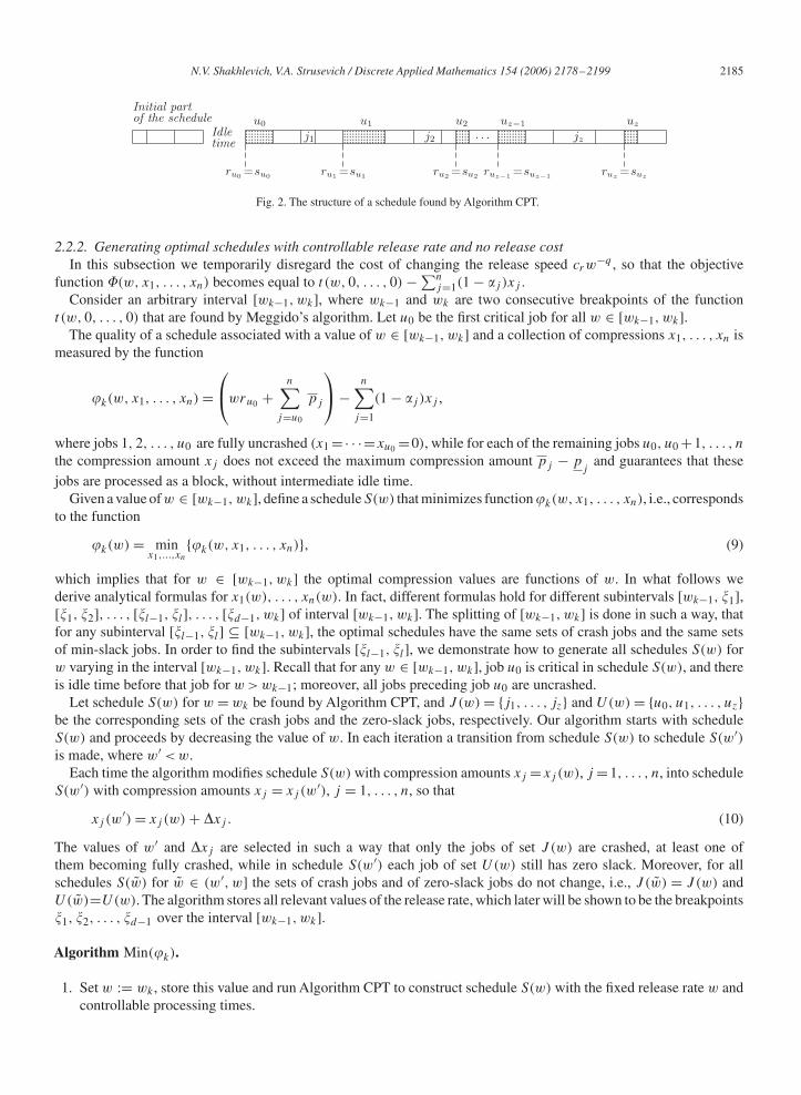
The running time of Algorithm CPT does not exceed O(n2).A typical structure of a schedule created by the algorithmis shown in Fig. 2. For our purposes two following types of jobs in that schedule are of special importance:

• zero-slack jobs u0, u1, . . . , uz;• crash jobs j1, . . . , jz.

Note that in the schedule found by Algorithm CPT, for each i, i�1, crash job ji is the first job in the set {ui−1, . . . , n}with the minimum compression cost �ji

, �ji< 1, which has not been fully crashed, i.e., pji

> pji

, and ui is the first jobwith zero slack, which follows ji . See [10] for an animated presentation of this algorithm.


Fig. 2. The structure of a schedule found by Algorithm CPT.

2.2.2. Generating optimal schedules with controllable release rate and no release costIn this subsection we temporarily disregard the cost of changing the release speed crw

−q , so that the objectivefunction �(w, x1, . . . , xn) becomes equal to t (w, 0, . . . , 0) −∑n

j=1(1 − �j )xj .Consider an arbitrary interval [wk−1, wk], where wk−1 and wk are two consecutive breakpoints of the function

t (w, 0, . . . , 0) that are found by Meggido’s algorithm. Let u0 be the first critical job for all w ∈ [wk−1, wk].The quality of a schedule associated with a value of w ∈ [wk−1, wk] and a collection of compressions x1, . . . , xn is

measured by the function

�k(w, x1, . . . , xn) =⎛⎝wru0 +

n∑j=u0

pj

⎞⎠−

n∑j=1

(1 − �j )xj ,

where jobs 1, 2, . . . , u0 are fully uncrashed (x1 =· · ·=xu0 =0), while for each of the remaining jobs u0, u0 +1, . . . , n

the compression amount xj does not exceed the maximum compression amount pj − pj

and guarantees that thesejobs are processed as a block, without intermediate idle time.

Given a value of w ∈ [wk−1, wk], define a schedule S(w) that minimizes function �k(w, x1, . . . , xn), i.e., correspondsto the function

�k(w) = minx1,...,xn

{�k(w, x1, . . . , xn)}, (9)

which implies that for w ∈ [wk−1, wk] the optimal compression values are functions of w. In what follows wederive analytical formulas for x1(w), . . . , xn(w). In fact, different formulas hold for different subintervals [wk−1, �1],[�1, �2], . . . , [�l−1, �l], . . . , [�d−1, wk] of interval [wk−1, wk]. The splitting of [wk−1, wk] is done in such a way, thatfor any subinterval [�l−1, �l] ⊆ [wk−1, wk], the optimal schedules have the same sets of crash jobs and the same setsof min-slack jobs. In order to find the subintervals [�l−1, �l], we demonstrate how to generate all schedules S(w) forw varying in the interval [wk−1, wk]. Recall that for any w ∈ [wk−1, wk], job u0 is critical in schedule S(w), and thereis idle time before that job for w > wk−1; moreover, all jobs preceding job u0 are uncrashed.

Let schedule S(w) for w = wk be found by Algorithm CPT, and J (w) = {j1, . . . , jz} and U(w) = {u0, u1, . . . , uz}be the corresponding sets of the crash jobs and the zero-slack jobs, respectively. Our algorithm starts with scheduleS(w) and proceeds by decreasing the value of w. In each iteration a transition from schedule S(w) to schedule S(w′)is made, where w′ < w.

Each time the algorithm modifies schedule S(w) with compression amounts xj =xj (w), j =1, . . . , n, into scheduleS(w′) with compression amounts xj = xj (w

′), j = 1, . . . , n, so that

xj (w′) = xj (w) + �xj . (10)

The values of w′ and �xj are selected in such a way that only the jobs of set J (w) are crashed, at least one ofthem becoming fully crashed, while in schedule S(w′) each job of set U(w) still has zero slack. Moreover, for allschedules S(w̃) for w̃ ∈ (w′, w] the sets of crash jobs and of zero-slack jobs do not change, i.e., J (w̃) = J (w) andU(w̃)=U(w). The algorithm stores all relevant values of the release rate, which later will be shown to be the breakpoints�1, �2, . . . , �d−1 over the interval [wk−1, wk].

Algorithm Min(�k).

1. Set w := wk , store this value and run Algorithm CPT to construct schedule S(w) with the fixed release rate w andcontrollable processing times.


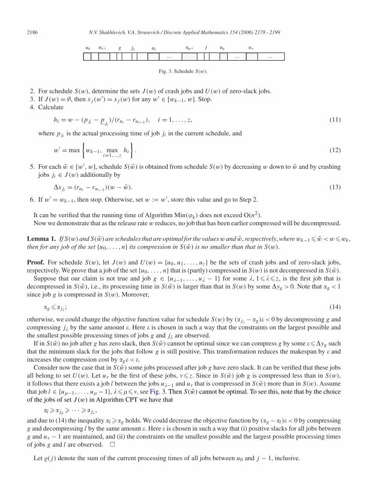
Fig. 3. Schedule S(w).

2. For schedule S(w), determine the sets J (w) of crash jobs and U(w) of zero-slack jobs.3. If J (w) = ∅, then xj (w

′) = xj (w) for any w′ ∈ [wk−1, w]. Stop.4. Calculate

hi = w − (pji− p

ji)/(rui

− rui−1), i = 1, . . . , z, (11)

where pjiis the actual processing time of job ji in the current schedule, and

w′ = max

{wk−1, max

i=1,...,zhi

}. (12)

5. For each w̃ ∈ [w′, w], schedule S(w̃) is obtained from schedule S(w) by decreasing w down to w̃ and by crashingjobs ji ∈ J (w) additionally by

�xji= (rui

− rui−1)(w − w̃). (13)

6. If w′ = wk−1, then stop. Otherwise, set w := w′, store this value and go to Step 2.

It can be verified that the running time of Algorithm Min(�k) does not exceed O(n2).Now we demonstrate that as the release rate w reduces, no job that has been earlier compressed will be decompressed.

Lemma 1. IfS(w)andS(w̃)are schedules that are optimal for the valuesw and w̃, respectively, wherewk−1 �w̃ < w�wk ,then for any job of the set {u0, . . . , n} its compression in S(w̃) is no smaller than that in S(w).

Proof. For schedule S(w), let J (w) and U(w) = {u0, u1, . . . , uz} be the sets of crash jobs and of zero-slack jobs,respectively. We prove that a job of the set {u0, . . . , n} that is (partly) compressed in S(w) is not decompressed in S(w̃).

Suppose that our claim is not true and job g ∈ {u�−1, . . . , u� − 1} for some �, 1��z, is the first job that isdecompressed in S(w̃), i.e., its processing time in S(w̃) is larger than that in S(w) by some �yg > 0. Note that �g < 1since job g is compressed in S(w). Moreover,

�g ��j� ; (14)

otherwise, we could change the objective function value for schedule S(w) by (�j� − �g)� < 0 by decompressing g andcompressing j� by the same amount �. Here � is chosen in such a way that the constraints on the largest possible andthe smallest possible processing times of jobs g and j� are observed.

If in S(w̃) no job after g has zero slack, then S(w̃) cannot be optimal since we can compress g by some ��yg suchthat the minimum slack for the jobs that follow g is still positive. This transformation reduces the makespan by � andincreases the compression cost by �g� < �.

Consider now the case that in S(w̃) some jobs processed after job g have zero slack. It can be verified that these jobsall belong to set U(w). Let u be the first of these jobs, �z. Since in S(w̃) job g is compressed less than in S(w),it follows that there exists a job l between the jobs u�−1 and u that is compressed in S(w̃) more than in S(w). Assumethat job l ∈ {u−1, . . . , u − 1}, ��, see Fig. 3. Then S(w̃) cannot be optimal. To see this, note that by the choiceof the jobs of set J (w) in Algorithm CPT we have that

�l ��j � · · · ��j� ,

and due to (14) the inequality �l ��g holds. We could decrease the objective function by (�g −�l )� < 0 by compressingg and decompressing l by the same amount �. Here � is chosen in such a way that (i) positive slacks for all jobs betweeng and u − 1 are maintained, and (ii) the constraints on the smallest possible and the largest possible processing timesof jobs g and l are observed. �

Let �(j) denote the sum of the current processing times of all jobs between u0 and j − 1, inclusive.


Theorem 1. Algorithm Min(�k) allows finding all optimal schedules for w running in the interval [wk−1, wk].The proof of this theorem is given in Appendix.Let �1, . . . , �d−1 be the increasing sequence of all values w′ generated and stored byAlgorithm Min(�k); additionally,

define �0 = wk−1 and �d = wk . It follows from the algorithm that for w ∈ [�l−1, �l] the sets J (w) and U(w) remainthe same; moreover, the optimal compressions xj depend on w linearly due to formula (10). This implies that function�k(w) is piece-wise linear over [wk−1, wk], and �0, . . . , �d are its breakpoints.

Theorem 2. Function �k(w) is convex over [wk−1, wk].Proof. To prove the convexity, we show that the slope of �k(w) increases monotonously over [wk−1, wk].

We compare the slopes of �k(w) for any two consecutive segments [�l−1, �l] and [�l , �l+1] and prove that

�k(�l ) − �k(�l−1)

�l − �l−1� �k(�l+1) − �k(�l )

�l+1 − �l

. (15)

Let xj (�l−1) and xj (�l ), j = 1, . . . , n, be the optimal compressions for w = �l−1 and w = �l , respectively. We havethat

�k(�l+1) − �k(�l ) =⎛⎝�l+1ru0 +

n∑j=u0

pj −n∑

j=1

(1 − �j ) × xj (�l+1)

⎞⎠

−⎛⎝�lru0 +

n∑j=u0

pj −n∑

j=1

(1 − �j ) × xj (�l )

⎞⎠ .

Let J (�l+1) = {j1, . . . , jz} and U(�l+1) = {u0, u1, . . . , uz}. Recall that only jobs ji ∈ J (�l+1) are subject tocompression while w decreases from �l+1 to �l . Due to (13), xji

(�l ) − xji(�l+1) = (rui

− rui−1)(�l+1 − �l ) so that wederive

�k(�l+1) − �k(�l ) = ru0(�l+1 − �l ) +z∑

i=1

(1 − �ji)(rui

− rui−1)(�l+1 − �l )

= (�l+1 − �l )

(ruz −

z∑i=1

�ji(rui

− rui−1)

).

The slope of function �k(w) for [�l , �l+1] is given by

H = ruz −z∑

i=1

�ji(rui

− rui−1). (16)

In a similar way, we can find the slope H ′ of function �k(w) for [�l−1, �l]; note that while H is determined for thesets J (�l+1) and U(�l+1), the value of H ′ is found with respect to the sets J (�l ) = {j ′

1, . . . , j′y} and U(�l ) = {u′

0 =u0, u

′1, . . . , u

′y}, where y�z. For simplicity, denote

J = J (�l+1), U = U(�l+1);

J ′ = J (�l ), U ′ = U(�l ).

It follows from Algorithm Min(�k) that U ′ ⊆ U . This means that u′y = u for some , 1��z.

To prove (15) we estimate the difference

H − H ′ =⎛⎝ruz −

∑ji∈J,ui∈U

�ji(rui

− rui−1)

⎞⎠−

⎛⎝ru′

y−

∑j ′i∈J ′,u′

i∈U ′�j ′

i(ru′

i− ru′

i−1)

⎞⎠ .


u0

u'0

u1 um um+1 um+b vu uz−1

… … …

u'µu'y

… …

u'µ +1

…

…

uz

(a)

(b)

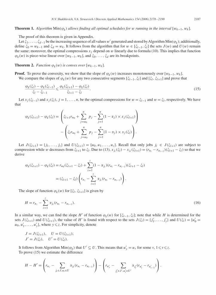
Fig. 4. Schedules (a) S(�l ) and (b) S(�l+1).

The two cases may occur.Case 1: If = z, i.e., u′

y = uz, then we obtain

H − H ′ =∑

j ′i∈J ′,u′

i∈U ′�j ′

i(ru′

i− ru′

i−1) −

∑ji∈J,ui∈U

�ji(rui

− rui−1).

It follows from Algorithm Min(�k) that for each pair of jobs u′ and u′

+1, there exist a pair of jobs um and um+b, suchthat um = u′

, um+b = u′+1. See Fig. 4. This implies that for any , 0��y − 1, the equality

ru′+1

− ru′= rum+b

− rum =m+b∑

i=m+1

(rui− rui−1)

holds. By the definition of the crash jobs, we have that �jm ��jm+1 � · · · ��jm+b��j ′

, and hence

�j ′(ru′

+1− ru′

) −

m+b∑i=m+1

�ji(rui

− rui−1) =m+b∑

i=m+1

(�j ′− �ji

)(rui− rui−1)�0. (17)

The latter inequality yields H − H ′ �0 and (15) is valid.Case 2: If < z, i.e., u′

y = u < uz, then we obtain

H − H ′ =(

ruz −∑

i=1

�ji(rui

− rui−1) −z∑

i=+1

�ji(rui

− rui−1)

)−⎛⎝ru −

∑j ′i∈J ′,u′

i∈U ′�j ′

i(ru′

i− ru′

i−1)

⎞⎠

=(

ruz −z∑

i=+1

�ji(rui

− rui−1) − ru

)+⎛⎝ ∑

j ′i∈J ′,u′

i∈U ′�j ′

i(ru′

i− ru′

i−1) −

∑i=1

�ji(rui

− rui−1)

⎞⎠ .

Since �ji< 1, the first term is positive. Besides, due to (17) the second term is non-negative. This implies that H −H ′ > 0

and (15) is valid. �

Remark 1. It follows from the proof of Theorem 2 that function �k(w) over each interval [�l , �l+1] is a linear functionwith a slope of H given by (16). Since all �ji

are less than 1, the value of H is positive for each interval [�l , �l+1], i.e.,�k(w) increases monotonously over [wk−1, wk].

2.2.3. Optimal scheduling with release costWe now turn back to the problem of minimizing the original function �(w, x1, . . . , xn) of form (7) over an interval

[wk−1, wk], 1�k�m+1. Recall that while the rate w varies within [wk−1, wk] the first critical job u0 does not change.For the last interval [wm, wm+1],where wm+1 is equal to a sufficiently large number W , there is only one critical

job u0 and all jobs u0, u0 + 1, . . . , n have equal release dates. The jobs u0, u0 + 1, . . . , n are processed as a block,


�0 = wk-1 �d = wk

ϕk (w)

Φk (w)

cw-q

w = �l�l-1

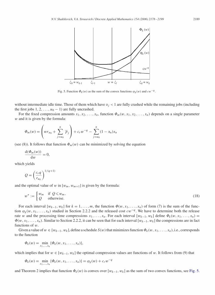
Fig. 5. Function �k(w) as the sum of the convex functions �k(w) and cw−q .

without intermediate idle time. Those of them which have �j < 1 are fully crashed while the remaining jobs (includingthe first jobs 1, 2, . . . , u0 − 1) are fully uncrashed.

For the fixed compression amounts x1, x2, . . . , xn, function �m(w, x1, x2, . . . , xn) depends on a single parameterw and it is given by the formula:

�m(w) =⎛⎝wru0 +

n∑j=u0

pj

⎞⎠+ crw

−q −n∑

j=u0

(1 − �n)xn

(see (8)). It follows that function �m(w) can be minimized by solving the equation

d(�m(w))

dw= 0,

which yields

Q =(

crq

ru0

)1/(q+1)

and the optimal value of w in [wm, wm+1] is given by the formula:

w∗ :={

wm if Q�wm,

Q otherwise.(18)

For each interval [wk−1, wk] for k = 1, . . . , m, the function �(w, x1, . . . , xn) of form (7) is the sum of the func-tion �k(w, x1, . . . , xn) studied in Section 2.2.2 and the released cost cw−q . We have to determine both the releaserate w and the processing time compressions x1, . . . , xn. For each interval [wk−1, wk] define �k(w, x1, . . . , xn) =�(w, x1, . . . , xn). Similar to Section 2.2.2, it can be seen that for each interval [wk−1, wk] the compressions are in factfunctions of w.

Given a value ofw ∈ [wk−1, wk], define a scheduleS(w) that minimizes function�k(w, x1, . . . , xn), i.e., correspondsto the function


{�k(w, x1, . . . , xn)},

which implies that for w ∈ [wk−1, wk] the optimal compression values are functions of w. It follows from (9) that


{�k(w, x1, . . . , xn)} = �k(w) + crw−q

and Theorem 2 implies that function �k(w) is convex over [wk−1, wk] as the sum of two convex functions, see Fig. 5.


Recall that function �k(w) is piecewise-linear over [wk−1, wk] and its breakpoints �0 = wk−1, �1, . . . , �d = wk canbe found by Algorithm Min(�k). Due to Remark 1, function �k(w) over an interval [�l−1, �l] for each l = 1, . . . , d,can be written as

�k(w) = Hw + crw−q + D,

where H is given by (16) and D does not depend on w, but may depend on l. The stationary point of �k(w) can befound by solving the equation

d(�k(w))

dw= 0,

which yields

Q =(crq

H

)1/(q+1)

. (19)

For minimizing function �k(w) we use the following method.

Algorithm Min(�k).

1. Use Algorithm Min(�k) for finding the increasing sequence of the breakpoints �0 = wk−1, �1, . . . , �d = wk offunction �k(w) over the interval [wk−1, wk].

2. Set l := d. Define w∗ := �l .3. Set w := �l . Determine the sets J (w), U(w). Find H by formula (16) and Q by formula (19). Define

w∗new :=

{�l−1 if �l−1 �Q,

�l if �l �Q,

Q if �l−1 < Q < �l

(20)

and update xji(w∗

new) = xji(w) + �xji

for all ji ∈ J (w), where

�xji= (rui

− rui−1)(w − w∗new),

leaving xj (w∗new) = xj (w) for all other jobs.

4. If w∗new = Q then output w∗

new, the corresponding schedule S(w∗new) and stop. Otherwise, if �k(w

∗new) < �k(w

∗)and l�2 then set w∗ := w∗

new, l := l − 1 and go to Step 3, else output w∗, the corresponding schedule S(w∗) andstop.

Algorithm Min(�k) scans the segment [wk−1, wk] by decreasing w starting from the right-hand endpoint. The valueof Q in Step 3 of the algorithm is a stationary point of the function �k(w) for w ∈ [�l−1, �l] where �l−1 and �l aretwo consecutive breakpoints of the function �k(w), see Fig. 5. In any iteration, the current value of w∗ delivers theminimum to the function �k(w) over the intervals considered so far. Similarly, w∗

new minimizes �k(w) over the currentinterval [�l−1, �l]. If w∗

new = Q then w∗new corresponds to the global minimum of the function �k(w) over [wk−1, wk],

since �k(w) is convex. If �k(w∗new) < �k(w

∗) and l =1, function �k(w) monotonously increases over [wk−1, wk], andthe algorithm finds w∗ = wk−1. If �k(w

∗new)��k(w

∗), then the function does not decrease as w decreases below w∗;due to convexity of �k(w) this implies that w∗ will deliver the minimum to the function over [wk−1, wk]. The lattercase includes the situation that the function is monotonously decreasing, so that the algorithm outputs w∗ = wk .

The running time of Algorithm Min(�k) does not exceed O(n2). Step 1 alone requires O(n2) time. Steps 3 and 4 arerepeated no more than n times. In each iteration, updating the sets J (w) and U(w) can be implemented in linear time.Finding H also takes O(n) time. Note that for the empty sets J (w) and U(w) formula (16) reduces to H = ru0 .

The results of this section can be summarized in the following statement.

Theorem 3. Algorithm Min(�k) determines the value of w that minimizes function �k(w) over the interval [wk−1, wk]in O(n2) time.


2.2.4. General algorithmWe present now the complete algorithm for solving the single machine problem with controllable release speed and

controllable processing times.

Algorithm CRS/CPT.

1. If necessary, renumber the jobs so that (1) holds.2. Run the algorithm by Meggido [18] and find all breakpoints w0, w1, . . . , wm of function �(w, 0, . . . , 0).3. Determine the optimum release rate w∗(m+ 1) in the last interval [wm, wm+1] using formula (18). Run Algorithm

CPT to find x∗1 (m + 1), . . . , x∗

1 (m + 1).4. For each k = m, m − 1, . . . , 2, 1 run Algorithm Min(�k) to find the optimal release rate w∗(k) and compression

amounts x∗1 (k), . . . , x∗

n(k). Compute �k(w∗(k), x∗

1 (k), . . . , x∗n(k)).

5. Find the value w∗ such that w∗ = w∗(h) for some h, 1�h�m + 1, where

�h(w∗(h), x∗

1 (h), . . . , x∗n(h)) = min

1�k �m+1�k(w

∗(k), x∗1 (k), . . . , x∗

n(k)).

6. Define v∗r = 1/w∗.

The running time of the algorithm is O(n3).

3. Controllable release dates

In this section we consider the situation related to the supply chain in Fig. 1 that the supplier is willing to modifyrelease dates for individual jobs. Recall that here job j ∈ N is given a ‘standard’ release date r̄j which can be reducedto the minimum value rj , where rj � r̄j . Reducing r̄j to some actual value rj , rj �rj � r̄j , incurs additional cost �j yj ,where yj = r̄j − rj is the compression amount of the corresponding release date.

3.1. Controllable release dates and constant processing times

In this subsection we assume that the job processing times p1, . . . , pn remain unchanged, i.e., modifying the jobrelease dates is the only type of coordination in the supply chain. Thus, our goal is to determine optimum releasecompression amounts y1, . . . , yn and an optimal permutation � = (�(1), �(2), . . . , �(n)) of jobs that minimize thefunction

F(�, y1, . . . , yn) = t (�, y1, . . . , yn) +n∑

j=1

�j yj . (21)

The first component of function F(�, y1, . . . , yn) represents the makespan, provided that the jobs are sequencedaccording to a permutation � and the release date of each job j is decreased by yj , i.e.,

t (�, y1, . . . , yn) = max1�u�n

⎧⎨⎩r̄�(u) − y�(u) +

n∑j=u

p�(j)

⎫⎬⎭ ,

while the second component is total compression cost.Suppose that the value of the makespan of a schedule that minimizes function (21) is known to be equal to Y .

Then the problem reduces to an auxiliary problem 1|rj − yj , Cmax �Y |∑ �j yj of finding the compression valuesy1, . . . , yn and the permutation of jobs that minimize the expression

∑nj=1 �j yj . The latter problem is equivalent to a

single machine problem PY to minimize total weighted tardiness, usually denoted by 1‖∑ wjTj , where the tardinessof job j that completes at time Cj with respect to a given due date dj is defined as Tj = max{Cj − dj , 0}. To see this,it suffices to modify Problem PY by changing the direction of time and by setting the weights wj equal to �j and thejob due dates equal to dj = Y − r̄j .


Since problem 1‖∑ wjTj is NP-hard in the strong sense [15], we obtain the following statement (see also [20] foran alternative proof).

Theorem 4. The single machine problem with controllable release dates to minimize function (21) is NP-hard in thestrong sense, even if the makespan of the optimal schedule is known.

Note that if all �j are equal, then the original problem in a similar way can be associated with a single machineproblem to minimize total (unweighted) tardiness, denoted by 1‖∑ Tj . Since the latter problem is NP-hard in theordinary sense (see [6]), we can conclude that the problem with controllable release dates and equal compression costs�j = � has the same complexity status. On the other hand, problem 1‖∑ Tj admits a pseudopolynomial dynamicprogramming algorithm by Lawler [15], and this allows us to use Lawler’s algorithm as a subroutine to obtain a solutionof the original problem with equal �j = � in pseudopolynomial time. The number of calls of Lawler’s algorithm doesnot exceed maxj∈N r̄j +∑

j∈N pj .

3.1.1. Controllable release dates and constant processing times: common boundsIn the remainder of this section we concentrate on the case that release dates have the same upper bound r̄ and

the same lower bound r . We assume that r̄ , r and all processing times are integer. In terms of the supply chain, thisassumption means that the supplier originally does not have any preferences regarding the order of releasing the jobs.By technological conditions, no job can be released earlier that time r; on the other hand, it is possible to release alljobs by time r̄ . The manufacturer accepts that some of the jobs are released at time r̄ , and negotiates with the suppliera suitable order of those jobs which will be released earlier than r̄ .

Let the jobs that become available earlier than time r̄ be called early jobs, while the other jobs are called late. Notethat the late jobs have a common release date r̄ , while for the early jobs the release dates are reduced individually.

Without loss of generality, we may assume that �j < 1 for all j = 1, . . . , n. Indeed, the release date of a job j with�j �1 will remain equal to r̄ in any optimal schedule.

We will distinguish between two versions of the problem: the unrestricted one for which the inequality

r̄ − r �n∑

j=1

pj (22)

holds and the restricted one for which (22) does not hold. Note that for the unrestricted version of the problem themanufacturer can schedule all jobs in the time interval [r, r̄], while in the restricted case that is not possible. Thus, theunrestricted version is easier to solve; in particular the NP-hardness of the unrestricted version of the problem wouldimply the NP-hardness of the restricted counterpart. Separate consideration of the restricted and unrestricted versionsof a scheduling problem is traditional for problems with a common due date, see, e.g., surveys [3,7].

As earlier in Section 3.1, we can associate the unrestricted version of the problem with common bounds on controllablerelease dates with a single machine problem to minimize total weighted tardiness with respect to a common due date,denoted by 1|dj = d|∑ wjTj . The latter problem is known to be NP-hard in the ordinary sense [25], and this impliesthe following statement.

Theorem 5. The single machine problem with controllable release dates to minimize function (21) is NP-hard inthe ordinary sense for both unrestricted and restricted cases even if the release dates have common bounds and themakespan of the optimal schedule is known.

We now present pseudopolynomial algorithms for both versions of the problem with common bounds for controllablerelease dates.

We start with the unrestricted case. Consider an optimal schedule S∗ associated with a permutation� = �(1), �(2), . . . , �(n) of jobs. In S∗ either all jobs are late or there is a sequence or early jobs �(1), . . . , �(k)

such that job �(k) completes exactly at time r̄ . If this property does not hold, then by performing an appropriate shift(to the left or to the right depending on the sign of k��(k) −1) we obtain a schedule with a smaller value of the objectivefunction. Thus, the original release date r̄ for job �(k) is reduced by y�(k) = p�(k), the release date for job �(k − 1)


is reduced by y�(k−1) = p�(k) + p�(k−1), and so on, the release date for job �(1) is reduced by y�(1) =∑kj=1 p�(j).

Hence, to minimize function (21) it suffices to minimize the function

f (�) = min1�k �n

⎧⎨⎩r̄ +

n∑j=k+1

p�(j) +k∑

j=1

��(j)

k∑i=j

p�(i)

⎫⎬⎭ (23)

over all permutations of jobs.If necessary, re-number the jobs in such a way that

p1

�1� p2

�2� · · · � pn

�n

, (24)

which corresponds to the well-known Smith rule [21]. It follows from [21] that in an optimal schedule early jobs mustbe sequenced in the order of this numbering.

Our pseudopolynomial dynamic programming algorithm for the problem of minimizing function (23) is based on abackward recursion. The jobs are scanned in the order opposite to their numbering. Suppose that jobs n, n−1, . . . , k+1have been assigned, and Fk+1(P ) is the value of the objective function, provided that total processing time of the earlyjobs is P , i.e.,

P =∑j∈E

pj ,

where E is the set of early jobs in the partial schedule. There are two options to schedule the next job k:

(i) Job k is scheduled late. Its exact position among other late jobs is immaterial. Scheduling job k does not affectthe set of early jobs, while the value of the makespan increases by pk , i.e.,

Fk(P ) = Fk+1(P ) + pk .

(ii) Job k is scheduled early. In this case job k is inserted before the first early job, which does not affect the makespan.The release date of each previously scheduled early job does not change, the release date of job k is reduced byyk equal to the total processing times of all early jobs, i.e.,

Fk(P ) = Fk+1(P − pk) + �kP .

The initial conditions are given by

Fn+1(P ) = r̄

for all P = 0, 1, . . . , p(N) =∑j∈N pj . The main recursion is given by

Fk(P ) = min{Fk+1(P ) + pk, Fk+1(P − pk) + �kP |k = n, n − 1, . . . , 1}.The algorithm stops having found

min0�P �p(N)

F1(P ).

The actual sequence of jobs corresponding to an optimal schedule can be found by backtracking. The running timeof the algorithm is O(np(N)).

Thus, we have proved the following statement.

Theorem 6. The unrestricted version of the single machine problem with controllable release dates, provided that allrelease dates have the same upper bound r̄ and the same lower bound r , is solvable in O(np(N)) time.

We now pass to considering the restricted version of our problem. As above, assume that the jobs are numbered inaccordance with (24).


Unlike the unrestricted case, there may exist a job h which straddles the release date r̄ , i.e., starts before and completesno earlier than time r̄ . The jobs that are processed before h are early and are sequenced in the order of their numbering.

Let in an optimal schedule S∗ the jobs follow the sequence � = �(1), �(2), . . . , �(n). Suppose that �(k + 1) = h isthe straddling job and the jobs �(1), . . . , �(k) are also early. If the original release date r̄ for job �(k + 1) is reducedby yh = y�(k+1), then the release date for job �(k) is reduced by y�(k) = yh + p�(k), and so on, the release date for job�(1) is reduced by y�(1) = yh +∑k

j=1 p�(j). Hence, to minimize function (21) it suffices to minimize the function

f (�) = min1�k �n−1

⎧⎨⎩r̄ + (p�(k+1) − y�(k+1)) +

n∑j=k+2

p�(j)

+k∑

j=1

��(j)

⎛⎝ k∑

i=j

p�(i) + y�(k+1)

⎞⎠+ ��(k+1)y�(k+1)

⎫⎬⎭ (25)

over all permutations of jobs. The compression amount yh may take any integer value from 1 till ph.For any h from 1 to n, let S(h, yh) define a schedule for processing a single job h in such a way that this job straddles

and is released at time r̄ − yh.For each combination of h and yh, our dynamic programming algorithm starts from schedule S(h, yh). Let the

sequence of the remaining n − 1 jobs taken in the order of their numbering be denoted by �(1), �(2), . . . , �(n − 1).These jobs are scanned according to the sequence �(n − 1), �(n − 2), . . . , �(1). Suppose that jobs �(n − 1), �(n −2), . . . ,�(k + 1) have been assigned, and Fk+1(P, h, yh) is the value of the objective function, provided that totalprocessing time of the jobs that precede the straddling job h is P . Define the room available for scheduling additionalearly jobs as

z = (r̄ − r) − P − yh,

and call this value the slack.There are two options to schedule the next job �(k):

(i) Job �(k) is scheduled late, i.e., after job h. This case is similar to the unrestricted version, so that

Fk(P, h, yh) = Fk+1(P, h, yh) + p�(k).

(ii) Job �(k) is scheduled early, i.e., before the first early job in accordance with (24). This is only possible if z�p�(k).The makespan does not change, the release date of job k is reduced by yk equal to the total processing times ofall early jobs plus yh. The value of z is decreased by p�(k).

Fk(P, h, yh) = Fk+1(P − p�(k), h, yh) + ��(k)P + ��(k)yh.

If both options are possible, the algorithm accepts the smaller of the found values Fk(P, h, yh).For every pair h and yh, where 1�h�n and 1�yh �pmax = max{pj |j ∈ N}, the initial conditions are given by

Fn(P, h, yh) = �hyh + r̄ + (ph − yh)

for all P = 0, 1, . . . , p(N) − ph.The algorithm stops having found

min{F1(P, h, yh)|0�P �p(N) − ph, 1�h�n, 1�yh �ph}.The actual sequence of jobs corresponding to an optimal schedule can be found by backtracking. The running time

of the algorithm is O(n2p(N)pmax).Thus, we have proved the following statement.

Theorem 7. The restricted version of the single machine problem with controllable release dates, provided that allrelease dates have the same upper bound r̄ and the same lower bound r , is solvable in O(n2p(N)pmax) time.


Finally, we show that the unrestricted version of the problem with common bounds on controllable release datesadmits a fully polynomial approximation scheme (FPTAS). Recall that for a minimization problem a FPTAS is a seriesof approximation algorithms which for any positive � generate a solution with the value of the objective function thatis at most (1 + �) times the optimal value, and with the running time that is polynomial with respect to both the lengthof the problem input and 1/�.

We formulate our scheduling problem as a special integer quadratic programming problem, known as positive half-product (PHP), which is a modification of the problem introduced in [2]. Problem PHP is a problem of minimizationthe function

H(z1, z2, . . . , zn) =∑

1� i<j �n

aibj zizj +n∑

j=1

hj (1 − zj ) +n∑

j=1

gj zj + D,

where zj ∈ {0, 1}, D�0, and all coefficients aj , bj , gj and hj are non-negative.A FPTAS for problem PHP is developedby Janiak et al. [14]. To see that our scheduling problem reduces to problem PHP, recall that the jobs are numberedin accordance with (24) and define the Boolean variable zj = 1 if job j is scheduled early and zj = 0, otherwise. Thecorresponding makespan can be written as r̄ +∑n

j=1 pj (1 − zj ), while the release date compression amount yi for anearly job i is equal to

∑ni=j pj zj , so that the overall objective function becomes

n∑i=1

�izi

⎛⎝ n∑

j=i

pizj

⎞⎠+ r̄ +

n∑j=1

pj (1 − zj ) =∑

1� i<j �n

�ipj zizj +n∑

j=1

pj (1 − zj ) +n∑

j=1

�jpj zj + r̄ ,

which is equivalent to function H with aj = �j , bj = pj , hj = pj , gj = �jpj and D = r̄ .

3.2. Controllable release dates and controllable processing speed: common bounds and equal compression costs

In this subsection we consider the situation that not only the supplier controls the job release dates, but also themanufacturer is ready to cooperate by modifying the machine processing speed. Due to the NP-hardness resultsestablished in Section 3.1, here we only consider the case that the release dates have a common upper bound r̄ and acommon lower bound r , and additionally all release date compression costs are equal, i.e., �j = �. Besides, we alsodistinguish between the unrestricted and restricted versions of the problem.

Assume that pj is a given ‘standard’ value of the processing time of job j and we can increase the speed at whichthe jobs are processed on the machine. If the processing speed is equal to vp then the processing time of job j ∈ N

equals wppj , where wp = 1/vp is the processing rate. Let wp be a fixed processing rate. Speeding up the machineincurs the processing speed cost cpw

−qp , where cp is a positive constant and q is a positive integer. We are looking for

a schedule that minimizes the sum of the makespan, total release date compression cost and the processing speed cost.We start with the unrestricted version first, for which condition (22) holds with respect to the standard processing

times. Assume that the jobs are numbered according to the LPT rule, i.e.,

p1 �p2 � · · · �pn.

Using the results from [5], we can derive that for any fixed processing rate there exists an optimal schedule in whichthe jobs are processed in the LPT order. Moreover, there are h = 1/�� early jobs and the job in position h completesexactly at time r .

For a schedule S associated with a fixed processing rate wp we have that

Cmax(S) = r +n∑

j=h+1

wppj ,

while total release date compression cost is given by �∑h

j=1∑h

i=j wppi . Hence, the objective function can be writtenas

F(wp) = r +n∑

j=h+1

wppj + �h∑

j=1

h∑i=j

wppi + cpw−qp


and this function has to be minimized with respect to its only controllable parameter, wp. Taking the derivative, weobtain

d(F (wp))

dwp

=n∑

j=h+1

pj + �h∑

j=1

h∑i=j

pi − qcpw−q−1p = 0,

so that the optimal processing rate w∗p satisfies

w∗p =

(qcp∑n

j=h+1 pj + �∑h

j=1∑h

i=j pi

)1/(q+1)

. (26)

The overall running time needed for finding w∗p and the corresponding optimal schedule is O(n log n) due to the

sorting of jobs in the LPT order.For the restricted version, the jobs in an optimal schedule still follow the LPT order, but there may exist a job that

straddles the release date r̄ . As in the restricted case, no optimal schedule may contain more than h = 1/�� early jobs.With the standard processing times, find how many jobs taken in the LPT order can fit into the interval [r, r̄] and

denote this number by m.For each job k, m�k�h, we determine the interval [w′

p(k), w′′p(k)] such that while wp varies within this interval

only jobs 1, 2, . . . , k are early with job k straddling. Note that

w′′p(k) = r̄ − r∑k

j=1 pj

= w′p(k − 1).

For wp ∈ [w′p(k), w′′

p(k)] the objective function becomes

F(wp) =⎛⎝r +

n∑j=1

wppj

⎞⎠+ �

k∑j=1

⎛⎝r −

j−1∑i=1

wppi

⎞⎠+ cpw

−qp .

The function is convex and can be minimized as follows. Taking the derivative, we obtain

d(F (wp))

dwp

=n∑

j=1

pj − �k∑

j=1

j−1∑i=1

pi − qcpw−q−1p = 0.

The root of this equation is given by

Q =(

qcp∑nj=1 pj − �

∑kj=1

∑j−1i=1 pi

)1/(q+1)

and the optimal value of the processing rate w∗p(k) over the interval [w′

p(k), w′′p(k)] satisfies

w∗p(k) =

⎧⎨⎩

w′p(k), if w′

p(k)�Q

w′′p(k), if w′′

p(k)�Q

Q, if w′p(k) < Q < w′′

p(k).

We find the values w∗p(k) for all k between m and h inclusive. Note that if the processing rate is further decreased,

for wp ∈ (0, w′p(h)] we obtain the situation similar to the unrestricted case. Therefore, we additionally compute w∗

p by(26) as in the unrestricted case and, if w∗

p(h) > w∗p, redefine w∗

p(h) := w∗p. An optimal processing speed corresponds

to the found value w∗p(k) that delivers the minimum to the overall cost F(wp). The running time of this algorithm

is O(n log n), since finding each of O(n) values w∗p(k) takes constant time, and all relevant values of F(wp) can be

computed in linear time.


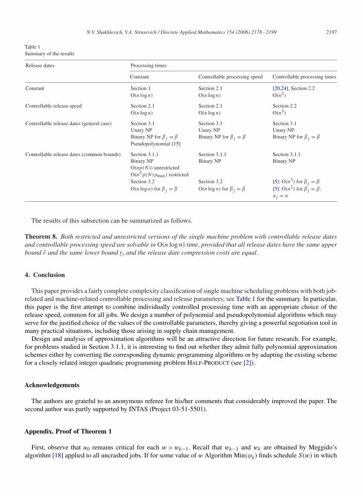
Table 1Summary of the results

Release dates Processing times

Constant Controllable processing speed Controllable processing times

Constant Section 1 Section 2.1 [20,24], Section 2.2O(n log n) O(n log n) O(n2)

Controllable release speed Section 2.1 Section 2.1 Section 2.2O(n log n) O(n log n) O(n3)

Controllable release dates (general case) Section 3.1 Section 3.1 Section 3.1Unary NP Unary NP Unary NPBinary NP for �j = � Binary NP for �j = � Binary NP for �j = �Pseudopolynomial [15]

Controllable release dates (common bounds) Section 3.1.1 Section 3.1.1 Section 3.1.1Binary NP Binary NP Binary NPO(np(N)) unrestrictedO(n2p(N)pmax) restrictedSection 3.2 Section 3.2 [5]: O(n3) for �j = �O(n log n) for �j = � O(n log n) for �j = � [5]: O(n2) for �j = �,

�j = �

The results of this subsection can be summarized as follows.

Theorem 8. Both restricted and unrestricted versions of the single machine problem with controllable release datesand controllable processing speed are solvable in O(n log n) time, provided that all release dates have the same upperbound r̄ and the same lower bound r , and the release date compression costs are equal.

4. Conclusion

This paper provides a fairly complete complexity classification of single machine scheduling problems with both job-related and machine-related controllable processing and release parameters; see Table 1 for the summary. In particular,this paper is the first attempt to combine individually controlled processing time with an appropriate choice of therelease speed, common for all jobs. We design a number of polynomial and pseudopolynomial algorithms which mayserve for the justified choice of the values of the controllable parameters, thereby giving a powerful negotiation tool inmany practical situations, including those arising in supply chain management.

Design and analysis of approximation algorithms will be an attractive direction for future research. For example,for problems studied in Section 3.1.1, it is interesting to find out whether they admit fully polynomial approximationschemes either by converting the corresponding dynamic programming algorithms or by adapting the existing schemefor a closely related integer quadratic programming problem HALF-PRODUCT (see [2]).

Acknowledgements

The authors are grateful to an anonymous referee for his/her comments that considerably improved the paper. Thesecond author was partly supported by INTAS (Project 03-51-5501).

Appendix. Proof of Theorem 1

First, observe that u0 remains critical for each w > wk−1. Recall that wk−1 and wk are obtained by Meggido’salgorithm [18] applied to all uncrashed jobs. If for some value of w Algorithm Min(�k) finds schedule S(w) in which


another job u′ > u0 is critical, then this schedule cannot be optimal, since some (partly) crashed job between jobs u0and u′ could be decompressed thereby decreasing the compression cost without increasing the makespan.

In all schedules found by Algorithm Min(�k) all jobs preceding job u0 remain uncrashed because their compressiondoes not decrease the makespan of the schedule but increases the compression cost. Therefore, while making transitionfrom schedule S(w) to schedule S(w′) only some jobs of the set {u0, . . . , n} could be subject to compression.

The algorithm starts with schedule S(wk) that is optimal since it is found by Algorithm CPT. Suppose that aftersome iterations schedule S(w) for wk−1 < w�wk is found and that schedule is optimal. We demonstrate that scheduleS(w′) found in the next iteration is also optimal.

For schedule S(w), let J (w) and U(w) be the sets of the crash jobs and the zero-slack jobs, respectively, and z bethe number of the crash jobs. If the value of w is decreased, the jobs of set U(w) receive a positive slack, so that thejobs of set J (w) can be further compressed. For each i, 1� i�z, Algorithm Min(�k) determines the value hi such thatthe slack of job ui with respect to the new release date hirui

remains zero, provided that job ji is fully crashed.Temporarily assume that there is no lower bound on possible values of the processing times.Take any w̃,wk−1 �w̃ < w.

Due to Lemma 1, the problem of finding an optimal schedule S(w̃) can be seen as the problem with controllable pro-cessing times and a fixed release rate w̃, provided that original processing times are equal to the current processingtimes in schedule S(w). This problem can be solved by Algorithm CPT. The algorithm will first take a compressible jobof set {u0, . . . , n} with the minimum compression cost no greater than 1 (this job will be job j1) and compress it till azero-slack job appears (this job will be job u1). In a similar way, job j2 will be found and compressed and a zero-slackjob u2 will be formed, etc. Thus, in transition from S(w) to S(w̃) only jobs j1, . . . , jz will be subject to compression.See [10] for an animated presentation of this discussion.

For each job ji ∈ J (w), the amount �xjiof this compression satisfies (10). Indeed, for each i, 1� i�z, the jobs

ui−1 and ui have zero slacks in both schedules S(w) and S(w̃). We obtain

wrui= wrui−1 + [�(ui) − �(ui−1)],

w̃rui= w̃ru−1 + [�(ui) − �(ui−1)] − �xji

,

so that (10) holds.In order to satisfy the lower bound restrictions on the processing times, we choose w′ as the smallest possible value

of w̃�wk−1, which guarantees that the compressions �xjiare all feasible. It follows from (10) and �xji

�pji− p

ji

that for each i, 1� i�z, the inequalities

w̃�w − (pji− p

ji)/(rui

− rui−1)

hold. Therefore, due to (11), the smallest value of w̃ is determined by (12). The theorem is proved.

References

[1] A. Agnetis, N.G. Hall, D. Pacciarelli, Supply chain scheduling: sequence coordination, Discrete Appl. Math., this issuedoi:10.1016/j.dam.2005.04.019.

[2] T. Badics, E. Boros, Minimization of half-products, Math. Oper. Res. 23 (1998) 649–660.[3] B. Chen, C.N. Potts, G. Woeginger, A review of machine scheduling: complexity, algorithms and approximability, in: D.-Z. Du, P.M. Pardalos

(Eds.), Handbook of Combinatorial Optimization, Kluwer, Dordrecht, 1998, pp. 21–169.[4] Z.-L. Chen, N.G. Hall, Supply chain scheduling: assembly systems, Working Paper, Fisher College of Business, The Ohio State University,

2001.[5] T.C.E. Cheng, M.Y. Kovalyov, N.V. Shakhlevich, Scheduling with controllable release dates and processing times: Makespan minimization,

European J. Oper. Res., to appear.[6] J. Du, J.Y.-T. Leung, Minimizing total tardiness on one machine is NP-hard, Math. Oper. Res. 15 (1990) 483–495.[7] V.S. Gordon, J.-M. Proth, C. Chu, A survey of the state-of-the-art of common due date assignment and scheduling research, European J. Oper.

Res. 139 (2002) 1–25.[8] N.G. Hall, Supply chain scheduling, in: Book of Abstracts of the International Symposium on Combinatorial Optimization, Paris, 2002,

pp. 10–11.[9] N.G. Hall, C.N. Potts, Supply chain scheduling: batching and delivery, Oper. Res. 51 (2003) 566–584.

[10] 〈http://staffweb.cms.gre.ac.uk/∼sv02/papers/animations1.html〉.[11] H. Ishii, T. Masuda, T. Nishida, Two machine mixed shop scheduling problem with controllable machine speeds, Discrete Appl. Math. 17

(1987) 29–38.[12] H. Ishii, T. Nishida, Two machine open shop scheduling problem with controllable machine speeds, J. Oper. Res. Soc. Japan 29 (1986)

123–131.

http://www.10.1016/j.dam.2005.04.019.

http://staffweb.cms.gre.ac.uk/sv02/papers/animations1.html


[13] A. Janiak, Single machine scheduling problem with a common deadline and resource dependent release dates, European J. Oper. Res. 53 (1991)317–325.

[14] A. Janiak, M.Y. Kovalyov, W. Kubiak, F. Werner, Positive half-products and scheduling with controllable processing times, European J. Oper.Res. 165 (2005) 416–422.

[15] E.L. Lawler, A ‘pseudopolynomial’ algorithm for sequencing jobs to minimize total tardiness, Ann. Discrete Math. 1 (1977) 331–342.[16] E.L. Lawler, J.K. Lenstra, A.H.G. Rinnooy Kan, D.B. Shmoys, Sequencing and scheduling: algorithms and complexity, in: S.C. Graves, A.H.G.

Rinnooy Kan, P.H. Zipkin (Eds.), Handbooks in Operations Research and Management Science, vol. 4, Logistics of Production and Inventory,North-Holland, Amsterdam, 1993, pp. 455–522.

[17] C.L. Li, Scheduling with resource dependent release dates—a comparison of two different resource consumption functions, Naval Res. Logist.41 (1994) 807–879.

[18] N. Meggido, Combinatorial optimization with rational objective functions, Math. Oper. Res. 4 (1979) 414–424.[19] E. Nowicki, An approximation algorithm for a single machine scheduling problem with release times, delivery times and controllable processing

times, European J. Oper. Res. 72 (1994) 74–81.[20] E. Nowicki, S. Zdrzałka, A survey of results for sequencing problems with controllable processing times, Discrete Appl. Math. 26 (1990)

271–287.[21] W.E. Smith, Various optimizers for single stage production, Naval Res. Logist. Quart. 3 (1956) 59–66.[22] V.A. Strusevich, Two machine flow shop scheduling problem with no-wait in process: controllable machine speeds, Discrete Appl. Math. 59

(1995) 75–86.[23] C.P.M. van Hoesel,A.P.M. Wagelmans, M. vanVliet,An O(n log n) algorithm for the two-machine flow shop problem with controllable machine

speeds, INFORMS J. Comput. 8 (1996) 376–382.[24] L.N. Van Wassenhove, K.R. Baker, A bicriterion approach to time/cost tradeoffs in sequencing, European J. Oper. Res. 11 (1982) 48–54.[25] J. Yuan, The NP-hardness of the single machine common due date weighted tardiness problem, Systems Sci. Math. Sci. 5 (1992) 328–333.

Documents

Single machine scheduling with controllable release and processing parameters