Single Machine Scheduling with Time Deteriorating Job Values

Single Machine Scheduling with Time Deteriorating Job ValuesAuthor(s): S. Raut, J. N. D. Gupta and S. SwamiSource: The Journal of the Operational Research Society, Vol. 59, No. 1 (Jan., 2008), pp. 105-118Published by: Palgrave Macmillan Journals on behalf of the Operational Research SocietyStable URL: http://www.jstor.org/stable/4622886 .

Accessed: 24/09/2013 01:34

Your use of the JSTOR archive indicates your acceptance of the Terms & Conditions of Use, available at .http://www.jstor.org/page/info/about/policies/terms.jsp

.JSTOR is a not-for-profit service that helps scholars, researchers, and students discover, use, and build upon a wide range ofcontent in a trusted digital archive. We use information technology and tools to increase productivity and facilitate new formsof scholarship. For more information about JSTOR, please contact [email protected].

.

Palgrave Macmillan Journals and Operational Research Society are collaborating with JSTOR to digitize,preserve and extend access to The Journal of the Operational Research Society.

http://www.jstor.org

This content downloaded from 147.126.1.145 on Tue, 24 Sep 2013 01:34:08 AMAll use subject to JSTOR Terms and Conditions

http://www.jstor.org/action/showPublisher?publisherCode=pal

http://www.jstor.org/action/showPublisher?publisherCode=ors

http://www.jstor.org/stable/4622886?origin=JSTOR-pdf

http://www.jstor.org/page/info/about/policies/terms.jsp


Journal of the Operational Research Society (2008) 59, 105 -118 O 2008 Operational Research Society Ltd. All rights reserved. 0160-5682/08 $30.00

www.palgravejournals.com/jors

Single machine scheduling with time deteriorating job values

S Raut1, JND Gupta2* and S Swami1

1Indian Institute of Technology, Kanpur India; and 2 University of Alabama in Huntsville, Huntsville, AL, USA

This paper considers the problem of scheduling n jobs on a single machine where the job value deteriorates with its starting time. The objective of the problem is to maximize the cumulative value of all jobs. The problem is motivated from the real-life applications, such as movie scheduling, remanufacturing of high-technology products, web object transmission, and banner advertising. Unrestricted, truncated, and capacity constrained job value functions are considered. Some special cases of the problem, such as the unrestricted linear job value function, are polynomially solvable. The general problem is shown to be unary NP-hard and is modelled as a time index integer program. For the NP-hard cases, several heuristics are proposed. Results of the empirical evaluation of the relative performance of the proposed heuristics on critical parameters are reported. Journal of the Operational Research Society (2008) 59, 105-118. doi: 10. 1057/palgrave.jors.2602303 Published online 1 November 2006

Keywords: movie theatre scheduling; single machine; deteriorating job values; capacity constraint; NP-hardness; heuristics; empirical results

Introduction

Traditional scheduling research assumes that the job values are independent of their start and finish times. However, there are practical situations where job values depend on the starting time of a job. For example, in a simplified version of scheduling movies in a theatre, the revenue generated from screening a movie depends on its starting time as the customer inter- est in a movie deteriorates with the passage of time (Swami et al, 1999). Even though the length of time for which a specific movie is shown is determined by the contract between the movie theatre and the distributor of the movie, movie scheduling decisions that determine their starting times can affect the total profits. In order to formulate and solve the movie theatre scheduling problem, therefore, we assume that all other decisions (like those discussed by Swami et al, 1999) have al- ready been made. It is desired to find the order in which these n movies should be screened so as to maximize total profit.

Several other practical situations fit the above de- scription including the remanufacturing environment with high-technology product (Fleischmann et al, 1997) and web object transmission (Xia and Tse, 2000). In such situations, it is advantageous to consider scheduling problems where job values deteriorate with job starting times and the objective is to find a schedule that maximizes the cumulative job values. Since there is only one machine (like the movie theatre), we consider the single machine scheduling problem with

deteriorating job values to maximize the aggregate value of all jobs. Following the three field notation of the scheduling problems by Lawler et al (1993), we will designate this problem as I I Vj(t) I max 1 Vj where Vj (t) is the value ofjobj if it starts at time t and 'max' is used to make clear that the objective is the maximization of value rather than minimizing cost.

Ignoring the capacity constraint, Fisher and Krieger (1981, 1984) proposed a heuristic algorithm for the nonincreasing concave job deterioration job value function. Their algorithm is based on the piecewise linear approximation and always obtains at least 2/3rd of the optimal cumulative job value. Voutsinas and Pappis (2002) developed a heuristic algorithm for the 11 Vj (t) = wj (t + pj) I max • Vj problem. However, the effectiveness of their algorithm to find an optimal solution decreases as the problem size grows. Heuristics developed for minimizing a general cost function by Alidaee (1991, 1993) can be used for solving the 11 Vj (t)l max E Vj problem considered in this paper. Apart from the above developments, the I Vj (t)l max E Vj problem has not received much attention

in the literature. For example, existing literature does not ad- dress the issue of the capacity constrained environment with deteriorating job value functions.

This paper considers the 11 Vj (t)I max 1 Vj problem with and without capacity constraints and shows that, except for some special cases, the general problem is unary NP-hard. In view of its NP-hard nature, heuristics for various forms of the I1 Vj (t)l max L Vj problem are developed and empirically evaluated.

The rest of the paper is organized as follows. We first deal with the problem formulation and complexity including the

*Correspondence: JND Gupta, College of Administrative Science, Uni- versity of Alabama in Huntsville, Huntsville, AL 35899, USA. E-mail: [email protected]



106 Journal of the Operational Research Society Vol. 59, No. 1

identification of polynomially solvable special cases and a dominance-based optimization algorithm. Heuristics to find optimal or near-optimal schedules for the Il Vj (t) I max 1 Vj problem are then described. After this, the results of the computational experiments for empirically evaluating the

proposed algorithms are reported and discussed. Finally, we conclude the paper with a summary and some fruitful directions for future research.

Problem formulation and complexity

In this section, we formulate the 11 Vj(t)l max Vj problem and show that the general problem is unary NP-hard. However, some special cases are polynomially solvable. To start the discussion in this section, we formally define the 1I Vj (t) I max E Vj problem and describe several types of job value functions analyzed in this paper. Then, we show that the

problem with equal processing times is polynomially solvable. Problems with unrestricted job value functions are considered next where it is shown that the 1l Vj (t)= wj - 1jtl max E Vj problem is polynomially solvable. Problems with exponential job value functions are shown to be unary NP-hard unless the

job value deterioration rate for all jobs is a constant. Utiliz-

ing these results, we then show that problems with truncated job value functions and/or capacity constraints are unary NP- hard even for linear job value functions. Finally, we describe a dominance algorithm to find an optimum solution to the I I Vj (t)I max E Vj problem.

Problem definition and job value functions

Let N = {1, 2,..., n} be the set of n jobs, available at time zero, that is to be processed on a single machine without in-

terruptions, preemption or inserted idle time. There are no

setup times. At any given time, the machine can process only one job. Associated with each job j E N is the processing time of pj and its value Vj (t) which is a non-increasing function of its starting time t. Because of the capacity constraints, the value of any job j may not exceed an upper limit Uj. It is desired to find a schedule that will maximize the total value of all jobs.

To define this problem, consider a schedule a =

(a(1), a(2) ...6, (n)) of n jobs. Then, the start time tj of

job a(j) is given by j-1

t(j) = E Pa(i) (1)

i=1

Therefore, the total value of schedule a is given by

Vc(a) =- {LVa)(tr(j))

} (2) j=1

Then, the problem considered in this paper is one of finding a schedule a such that V () calculated using Equations (1) and (2) is maximum.

The value function of each job j, Vj could take various forms. In this paper, we consider cases involving linear and

exponential job value functions. Problems involving no capacity constraints are called the unrestricted job values. How- ever, in several situations, the job value may deteriorate up to some time and remain constant after that time. We call this type of job values truncated job values. Further, there may be an upper limit on the value of a job due to certain restrictions, like the maximum number of seats available in a movie theatre. These type of job value functions will be called capacity constrained job values. Based on the above discussion, representative job value functions can be shown in Figure 1.

In this paper, we focus on these cases of job value functions.

Problems with equal processing times

While the general problem is shown to be unary NP-hard later in this section, the equal processing time problem can be polynomially solved as shown below.

Theorem 1 The I I Vj (t), pj = p VjlI max E Vj problem is optimally solvable in O(n3) computation steps by solving an assignment problem.

Proof Since the processing times of all jobs are equal, the starting time of the job at sequence position i is (i - 1) * p, where i = 1,..., n. Introduce assignment variables xij (i, j =

1, ..., n), such that, xij = 1 if job j is assigned to sequence position i and = 0 otherwise. The problem can be formulated as follows:

n n

max ij * Vj((i

- 1)* p) (3) i=1 j=1

subject to: n

xij = 1, Vj = 1, 2 ...

, n (4)

n

xij = 1, Vi = 1, 2 ....,

n (5) j=1

xij E {0, 1, Vi = 1, 2 ..., n, j = 1, 2 ..., n (6)

The above optimization problem represented by Equations (3)-(6) can be converted into an equivalent standard linear as-

signment problem by subtracting each value Vj ((i - 1) * p) in the objective function in Equation (3) from

maxj n (V j(O)). This assignment problem can be formulated in O(n2) computational steps and solved in O(n3) computational steps (Lawler, 1976). O

Unrestricted job value functions

We now resolve the complexity of the I Vj (t) max C Vj problems starting with those involving unrestricted job value functions.

Unrestricted linear job value functions. We first consider the 1I Vj (t) = wj - 1jt max E V1 problem with unrestricted



S Raut et al-Single machine scheduling 107

Deterioration Function Function Expression Decay Pattern

Linear Function Vj(t) = wi- it

Vi(t)

t Exponential Function v (t) = wje i

/V(t)

t -(

TruncatedLinear Functi on V, (t) =max (vU, w - t)w

v (t)

t with Lm

Truncated Exponential V, (t) = max(v, we )) Function Wti

v (t)

Linear Function with V (t) = min (U, wj - Ajt) Wi Limited Capacity

V(t)U 7 t

Exponential Function with V-(t)

min(U, w e-t) wi Limited Capacity

V (t)

t -

Truncated Linear Function Vj (t) = min (U, max (v,, wj - jt)) w .. with Limited Capacity

U V (t)

v

t Truncated Exponential VI (t) = min (U, max(v , we-' )) wi Function With Limited

(

Capacity U

V (t)

t

Figure 1 Representative job value deterioration functions.

linear job value function where the value of job j starting at time t is given by Vj (t) = wj - )j t. In order to ensure that

job values are not negative, it is assumed that for each job j, wj, lj > 0 and wj ? )j(P - pj) where P =

En,=ps .

Theorem 2 The 1 IVj (t) = wj - j t max Vj problem is optimally solvable in O(n log n) computation steps by arranging jobs in descending order of the j /pj values.

Proof Let a=(a(1), a(2),..., a(n)) be a schedule of njobs where ca(j) represents job in sequence position j. Further,

let Ca(j) be the completion time of job a(j). Then, using Equations (1) and (2), the value of schedule a, V(a) is given by

n n

V(a) = E{wa( + 2+()PU(j)}

- L{AY(j)Ca(j)} (7)

j=1 j=1

From Equation (7) above, it is clear that V (a) is maximized by minimizing E•= {(jaC,(j)C)}, which is the sum of the weighted completion times of all jobs. Therefore, this problem is polynomially solvable in O(n log n) computation steps




using Smith's (1956) rule by arranging jobs in descending order of the Aj/pj values. D

During the application of Theorem 2 above (or heuristics based on similar analysis discussed in a later section), there

may be ties that do not cause any problem and can be re- solved arbitrarily. However, for its extension to other cases, appropriate tie-breaking rules are required. Therefore, in im-

plementing Theorem 2, we break ties in favour of a job with maximum wjl/pj value first, maximum wj value second, and maximum ,j value last. However, in case of equal values for all parameters, we select the job randomly.

Unrestricted exponential job value functions. The value of

job j is given by

Vj(tj) = wje-A2tj (8)

where Vj (tj) is interpreted as a job value deteriorating function, tj is the starting time, and wj, )j > 0. The objective function of the problem is as follows:

n n

E Vj(tj) = [wje-2;tj] (9)

j=1 j=1

Before resolving the complexity of the general 1I V(t) =

wje-ti I max Vj

problem, we note that through a simple job interchange argument, the following special case can be

polynomially solved.

Theorem3 The lIVj(t)=wje-At max Vj problem is optimally solvable in O(n log n) computation steps by arranging jobs in descending order of wj /(1 - e-APJ) values.

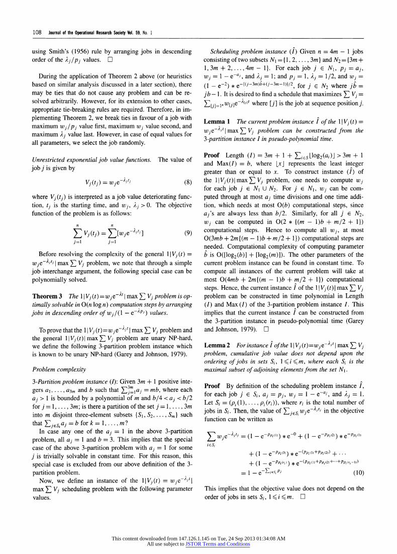
To prove that the 1 V1 (t)=wje-Atl max 1 V1 problem and the general I1 Vj(t)l max ~ Vj problem are unary NP-hard, we define the following 3-partition problem instance which is known to be unary NP-hard (Garey and Johnson, 1979).

Problem complexity

3-Partition problem instance (I): Given 3m + 1 positive inte-

gers al,..., a3m and b such that E mla = mb, where each aj > 1 is bounded by a polynomial of m and b/4 < aj < b/2 for j= 1 ..., 3m; is there a partition of the set j= 1 ..., 3m into m disjoint three-element subsets { Si, S2 ..., Sm } such that yjeskaj = b for k = 1 ..., m?

In case any one of the aj = 1 in the above 3-partition problem, all a1 = 1 and b = 3. This implies that the special case of the above 3-partition problem with aj = 1 for some j is trivially solvable in constant time. For this reason, this special case is excluded from our above definition of the 3- partition problem.

Now, we define an instance of the 1IVj(t)= wje-ljt max C Vj scheduling problem with the following parameter values.

Scheduling problem instance (I) Given n = 4m - 1 jobs consisting of two subsets N1 ={1, 2, ..., 3m) and N2= {3m + 1, 3m + 2,...,4m - 1}. For each job j e N1, pj = aj, wj = 1 - e-aJ, and ,j = 1; and pj = 1, =j = 1/2, and wj =

(1 - e-2) * e-{(j-3m)b+(j-3m-1))/2, for j E N2 where jb =

jb - 1. It is desired to find a schedule that maximizes 1 Vj =

Y[j]=1 lw[j]e-ijlt where [j] is the job at sequence position j.

Lemma 1 The current problem instance I of the 1 Vj (t) =

wje-jt I max Vj problem can be constructed from the 3-partition instance I in pseudo-polynomial time.

Proof Length (I) = 3m + 1 + •~Es[log2(ai)] > 3m + 1 and Max(I) = b, where [x] represents the least integer greater than or equal to x. To construct instance (I) of the 1I Vj(t)I max E Vj problem, one needs to compute wj for each job j E N U N2. Forj E N1, wj can be com-

puted through at most aj time divisions and one time addition, which needs at most O(b) computational steps, since

aj's are always less than b/2. Similarly, for all j E N2,

wj can be computed in 0(2 * {(m - 1)b + m/2 + 1}) computational steps. Hence to compute all w j, at most 0(3mb + 2m{(m - 1)b + m/2 + 1)) computational steps are needed. Computational complexity of computing parameter b is O([log2(b)] + [log2(m)]). The other parameters of the current problem instance can be found in constant time. To

compute all instances of the current problem will take at most 0(4mb + 2m{(m - 1)b + m/2 + 1}) computational steps. Hence, the current instance I of the I I Vj(t)I max 1 Vj problem can be constructed in time polynomial in Length (I) and Max (I) of the 3-partition problem instance I. This

implies that the current instance I can be constructed from the 3-partition instance in pseudo-polynomial time (Garey and Johnson, 1979). O

Lemma 2 For instance I of the 1I Vj (t)=wje-2;Jt I max E V1 problem, cumulative job value does not depend upon the ordering of jobs in sets Si, 1 <i <im, where each Si is the maximal subset of adjoining elements from the set N1.

Proof By definition of the scheduling problem instance I, for each job j E Si, aj = pi, wj

= 1 - e-a, and ,j = 1.

Let Si = (Pi(1) .... Pi(ri)), where ri is the total number of jobs in Si. Then, the value of js, wJe- t' in the objective function can be written as

C wje-'jtJ = (1 - e-Ppi"') * e-o + (1 - e-Ppi(2)) * e-Ppi()

isSi

+ (1 - e-piP3) * e-(ppi)-+Ppi(2))

...

+ (1 - e-ppi(ri) * e-(Ppi(l)+Ppi(2)++Ppi (ri-))

= 1 - e-EEsi PJ (10)

This implies that the objective value does not depend on the order of jobs in sets Si, 1 (ii (m. O




I S, 13m+ll S m+ S3 I ........ S- 4m-1I S, I

0 b+1 2b+2 3b+3 (m-2) b+ m-2 (m-1)b+ m-2 mb+ m-I

Figure 2 A possible solution of the 3-partition problem.

Lemma 3 In an optimal schedule for instance I of the I Vj(t) = wje-Ajtl max V1 problem, job j E N2 starts at time tj = {(j - 3m)b + (j - 3m - 1)} + 1 irrespective of the ordering of jobs in subset N1.

Proof Suppose that in an optimal schedule for instance i, job i E N1 immediately follows job j E N2. Then,

wj * ej(t)- wej e-*j(t+p;)

wi * e-2i(t)

- Wi * e-2i(t+pj)

Substituting the parameter values from the definition of the problem instance I in Equation (11), we get

t >{(j - 3m)b + (j - 3m - 1)} + 1 + 2A (12)

where

A = {ln(l + e-p/2) - ln(l + e-)} (13)

Since, by definition, pi > 1 for i E N1, it follows that

- < A < 0. In addition, as each pi is an integer, the starting times of all jobs will be integers. Further, in order to optimize the cumulative job value, starting time of job j, while satisfying condition (12) should be as small as possible. Therefore, in an optimal schedule, job j E N2 starts at time tj given by

tj = {(j - 3m)b + (j - 3m - l)} + 1 (14)

From Equation (14), it is clear that the starting time of job j e N2 does not influence the order of jobs in subset N1 nor is influenced by them. D

Theorem 4 The 1VjV(t) = wje-At'lmax E Vj and I I Vj (t) l max E Vj problems are unary NP-hard.

Proof The processing order and starting times of jobs N2 are obvious because of their parameters and Lemma 3 above. Therefore, filling other jobs in the time gaps created by the schedules of jobs in N2 will improve the objective function value. With this viewpoint, we consider a complete schedule as shown in Figure 2 where the processing order of jobs will be ({ili e SI}, 3m + 1, {ili E S2}, 3m + 2, {ili E S3} ..., 4m - 1, {ili E Sm}), where S= {S, S2,..., Sm} = {1...3m}.

From Figure 2, it follows that the starting time of job 3m + 1 is between b and iEs, ai - b = L1. The starting time of job 3m + 2 is between 2b + 1 and ZiEsus2a; + 1 - 2b - 1 = L2. Similarly, the starting times of jobs 3m + 3 ...., 4m - 1, will deviate from points 3b+ 2 ..., mb+m - 1 by L3 ..., Lm-1. From Lemma 2 it follows that the value of

_j swje-t)r

is not influenced by the ordering of jobs within the sets

S1, S2, ..., Sm. Further, from Lemma 3, it is clear that the ordering of jobs within sets S1, S2 ..., Sm is not influenced by

the jobs in subset N2. Using Lemma 2, the objective function for the scheduling problem instance I defined by Equation (9), Z =

LjeNN,UN2 we-t'iJ can be written as

Z = 1 - e- EjES aj + W3m+l * e-((b+L*)/2)

+ e-(EjEsaj+l) _ e-( jessus2aj+l)

+ W3m+2 * e-((2b+l+L2)/2) + e-(CtS jus2aj+2)

.. . . - e-( EjSI S2U...USm_

aj+m-2)

+W4m-1 e-((mb+m-l+Lm1_)/2) +e-(E•jsius...USm_ a+m-1)

- e-(EjEsaj+m-1)

= 1 - e-EjEsaj + e-(IEslaj+l) + W3m+1 * e-((b+LI)/2)

_ e-( Ejs,uS2aj+l) + e-(ZjESlUS2a

+2)

+ W3m+2 * e-((2b+1+L2)/2)_ ....

-e( ESIuus2...USm-l a+m-2)

+ e-(ESIUS2U...USms

aj+m-1)

+ W4m-1 * e-((mb+m-l+Lm-,)/2) _ e-(Ejesaj+m-1)

= 1 - (1 - e-) * e(b+L) + W3m+l * e-((b+LI)/2)

- (1 - e-1) * e-(2b+l+L2) + W3m+2 * e-((2b+l+L2)/2)

- ... - (1 - e-1) * e-(m-1)b+m-2+Lm-l

+ W4m-1 * e-((m-1)b+m-2+Lm-,)/2) _ e-(EjEsaj+m-1)

= 1 - e-(•E•saj+m-1)

- (1 - e-1)

x[{e-(b+Ll) }3m+l

*e-(b+L )/2

-

e-(2b+I+L2) _ W3m+2

*e-(2b+1+L2)/2 I (1- ee-1)

(1-e-1)

(15)

which simplifies to

Z = - e-(ESa+m-1)

W3m+k =1 e(.sa+m-)

+ k=1 4(1 - e-1)

m-1 e-Lk/2 e-1/2

kk= -

S(e-Lk/2 e+1/2 ] (16)

Since pj and b are integers, Lk must be integer. Therefore, from Equation (16), it is clear that the objective function Z increases as I LkI decreases. Hence, the objective function Z will be maximum at ILk =0 (Vk= 1, 2 ...., m- 1). Therefore,




substituting Lk = 0 in Equation (16), the optimal value of the

objective function Z* is given by

m-1 2

Z* = 1 - e-(Ejesaj+m-1) ? + E 3m+k e-')

k=l(1 - e

x e-(kb+k-1) 1 - /2 + e/2 (17)

k=12

Now, if the 3-partition instance I has a solution, then

ZjEskaj =b and ILk =0 Vk <sm. Therefore, the correspond-

ing scheduling problem instance I has an optimal solution with value Z* given by Equation (17).

Conversely, if the scheduling problem instance I has an

optimal solution with value Z* given by Equation (17), then Zjskaj = b and ILkl = 0 Vk <m. Further, since

b/4 < aj < b/2 for j = 1,...,3m, it follows that each Sk contains exactly three elements. Therefore, the subsets

S1, S2, ...,

Sm is a solution to the 3-partition instance I. Since the 3-partition problem is known to be unary NP-hard, and that the scheduling problem instance I can be constructed from the 3-partition instance I in pseudo-polynomial time (Lemma 1 above), using the results in Garey and Johnson (1979), it follows that the 1IVj (t) = wje-jt l max E

Vj and

II Vj (t)J max E Vj problems are unary NP-hard. EO

Theorem 4 above can be used to resolve the complexity of several other forms of exponential deterioration function as shown by the following corollary.

Corollary 1 The 1Vj (t) = wju-2At, u > 11

maxE Vj and

1iVj(t) = wju-At, uj > 1 Vj I max E Vj are unary NP-hard.

Truncated job value functions

We now consider the problem where the value of jobj remains constant after a certain time. In other words, we consider the

job value function of the form, Vj (t) = max(vj, fj(t)) where

fj (t) is a nonincreasing function of the start time t of job j and vj = fj (Tj) for some starting time Tj of job j. In other words, the value of a job j deteriorates only up to time Tj and not after that time.

We now show that 1Vj (t) = max(vj, fj(t)) Imax L Vj problem is unary NP-hard for any nonincreasing job value function.

Theorem 5 The 1IV1(t) = max(vj, f(t))l max Vj problem is unary NP-hard for any non-increasing job value function.

Proof To prove this theorem, consider the I Vj (t) =

max(vj, w1 - )jt)l maxE Vj problem where for each job j, vj = wi - jTj. Suppose that in an optimal schedule, subset of jobs started on or before time T1 is

r1 and those

started after time Tj

is r2. Define the deadline of job j, time by which job j must be completed,

dj as follows:

dj = Tj + pj if j E q, and dj = oo if j e /12 Then, using the developments similar to those in the proof of Theorem 2, it follows that the problem of finding an optimal schedule for the two subset of jobs r, and q/2 is equivalent to the 1 Id1 I E wj Cj problem (single machine problem to minimize

weighted flowtime subject to deadlines) which is known to be unary NP-hard (Lenstra et al, 1977). Since this subset of the special case of the II Vj (t) = max(vj, fj (t))l max E Vj problem is unary NP-hard, it follows that the general

Il Vj (t) = max(vj, fj (t))l max E Vj problem is unary NP- hard for any nonincreasing job value function. O

Capacity constrained job value functions

We now consider problems where capacity constraints causes an upper limit U on the value that a particular job can create. Therefore, the capacity constrained job value function may be represented as follows:

Vj(t) = min(U, f j(t)) (18)

where fj (t) is the unconstrained job value function. If U < minj <,n f (P - mini Pi) where P = I1 pi, then

any sequence is optimal. Further, if U > maxj <<nfj(0), the

problem reduces to the I Vj (t) = fj (t)l max E Vj problem whose complexity has been established above. Therefore, in this section, we consider the non-trivial case of the capacity constrained problem where U does not satisfy the above constraints.

Theorem 6 The 1I Vj(t) = min(U, fj (t)) max ~ Vj problem is unary NP-hard for any non-increasing job value

function.

Proof Consider a special case of this problem where Vj (t)= min(U, wj - ?jt) and U =

wj -

Jj Tj. Then, the job value function can be written as

Vj(tj) = min(0, -Xjtj ++ j Tj) + U

= U - max j(tj - Tj, 0) = U - max 1j (tj + pj - (Tj + pj), 0) (19)

Let Cj = tj + pj be the completion time of job j and define

dj = Tj + pj as its due date. Then, the I Vj (t) = min(U, wj - ljt)l max y Vj problem is equivalent to the 1 II u w; Tj (single machine weighted tardiness) problem which is known to be unary NP-hard (Lawler, 1977; Lenstra et al, 1977). There- fore, the 1IV1(t)=min(U, fj (t)) I max E V1 problem is unary NP-hard for any non-increasing job value function. O

Capacity constrained truncated job value functions

The objective function of the capacity constrained problem with truncated job value function is as follows:

_ V1(tj)

= min{U,

max(vj,

f1(t))} (20) j=1 j=1




If U < minji ~nvj, then any sequence is optimal. For other values of U, we now state the problem complexity.

Theorem 7 The 11Vj(t)=min{U, max(vj, fj(t))}I max E Vj problem is unary NP-hard.

Proof Follows from Theorems 6 above since the I Vj (t) = min{U, fj(t)} max ~Vj problem is special case of the

1lVj(t) = min{U, max(vj, fj(t))}J max Z Vj problem. O

Time index formulation

The above problem, regardless of the form of the job value function, can also be formulated as a mixed linear integer program (Sousa and Wolsey, 1992). To do so, for each job j, let xjt = 1, if job j is started at time t; and 0 otherwise. Further, let

n

P = Pi j=1

The problem then may be represented as the following integer program:

n P-Pj

max1 1 Vj (t). xjt (21) j=1 t=O

Subject to

P-pj

E xjt = 1, Vj = 1, 2, ... ,n (22) t=O

n t

E xj, 1, Vt = 1, 2,..., P (23) j=1 s=t-pj

xjt E {0o, Vj= 1,29....,n,

t = 1, 2, ...., P - pj (24)

The first set of equations ensures that each job is scheduled exactly once, whereas the second set of inequalities ensures that at each time, at most one job is executed.

Dominance algorithm

We now describe an optimization algorithm to solve the 1 V (t)l max C Vj problem. For this purpose, let V(a) be the total value of a partial (or complete) schedule a containing k jobs expressed as follows:

k

V(a) = {Va(i)(ta(i))

(25) i=1

Now consider two partial schedules a and a' that are different permutations of the same subset of jobs. Then, we state the following known result.

Theorem 8 For any schedules a and a' that are different permutations of the same subset ofjobs, V (a) < V (a') implies V(a97) < V('n).

A schedule a satisfying the conditions of Theorem 8 is said to a dominates schedule a'. Based on this, a pure dominance theorem to optimally solve the ll Vj(t)l max Vj problem can be described as follows.

Pure dominance algorithm Step 0: Let L = 1 and S= {1, 2, ..., n} be the set of n partial

schedules each consisting only of one job j E N. Compute V(p) Vp e S. Enter Step 1.

Step 1: For each partial schedule p e S, form n - L partial schedules consisting of L + 1 jobs by assigning each of the n - L unassigned jobs at sequence position L + 1. Let the set of partial schedules so formed be S. Compute V(p) Vp E S.

Step 2: Group the partial schedules containing the same subset of jobs together, that is, let S = { S, S2, ..., Sk }, where for each i < k, Si contains all partial schedules containing the same subset of jobs. For each subset Si, retain the partial schedule Pi with maximum V (Pi) value, that is, find pi e Si such that V(pi) = maxp js, V(pj). Enter Step 3.

Step 3: Let L =L + 1. If L < n, return to Step 1. Otherwise STOP; the last schedule retained in Step 2 is optimal.

While the above algorithm will optimally solve the

Il Vj (t)l max E Vj problem, it is, however, not likely to be an efficient algorithm. Its computational burden is exponential as in the best case, it will retain

r {n Cr } partial schedules.

Proposed heuristics

In view of the NP-hard nature of the problem, we present several heuristics that are based on existing literature. Since several existing algorithms can be used for problems with linear job value functions (by considering their minimum counter- parts), we concentrate on developing heuristics for the nonlinear job value functions.

Heuristics for unrestricted job value functions

Our first set of heuristics is an adaptation of greedy algorithms. At any sequence position, a greedy selection rule is used to assign a job to that sequence position. The basic steps of this greedy algorithm are as follows:

Algorithm G: basic greedy algorithm Step 0: Let t = 0, U= N= {1, 2 ..., n}, and S= 0. Enter

Step 1. Step 1: Let j be the job to be assigned to current sequence

position using some selection rule. Enter Step 2. Step 2: Set S = (S, j), U = (U\j), t = t +

pj, and enter

Step 3. Step 3: If U = 0, find V(S) using Equations (1) and (2)

and STOP, otherwise return to Step 1.

Algorithm G has a computational complexity of O(n2).




It remains to specify the selection rule used in Step 1 of the above algorithm. We now describe several rules to select job j to be assigned to a sequence position in Step 1 above.

Our first heuristic selects a job with maximum job value per unit time at a particular time t.

Algorithm H: highest value heuristic Step 1: Let j = arg[maxiu(Vi (t)/pi)] using appropriate

tie-breaking rules. Enter Step 2.

Our next heuristic follows the work of Fisher and Krieger (1981, 1984). This algorithm creates a dynamic job savings index for scheduling a job at time t rather than at the end of the schedule. To describe this algorithm, let P =

LEiNPi" Algorithm F: Fisher's greedy algorithm Step 1: Let j = arg[maxi~E(Vi(t) - Vi(P - Pi)/Pi)] using

appropriate tie-breaking rules. Enter Step 2.

Alidaee (1993) suggests to approximate Vj (t) by a contin- uous function over time and hence makes decisions based on the rate of value deterioration rather than the absolute value. To describe this algorithm, let Vj(t) be the differential of the

job value function with respect to t. Step 1 of this algorithm can be described as follows:

Algorithm A: Alidaee's differential algorithm Step 1: Let j = arg[miniu(Vi'(t)/pi)] using appropriate

tie-breaking rules. Enter Step 2.

Computational experience with algorithm A showed that it did not yield good results. However, its application in reverse, namely using the job selection rule from the last sequence position to the first produced excellent results. Therefore, we describe this revised algorithm as follows.

Algorithm R: Alidaee's reverse differential algorithm Step 0: Let t= P, U= N= {1, 2, ..., n), and S= 0. Enter

Step 1. Step 1: Let j=arg[miniu (Vi'(P-t)/pi)] using appropriate

tie-breaking rules. Enter Step 2. Step 2: Set S = (j, S), U = (U\j), t = t - pj, and enter

Step 3. Step 3: If U = 0, find V(S) using Equations (1) and (2)

and STOP, otherwise return to Step 1.

For the linear job value function, algorithms A and R described above generate an optimal schedule as they imple- ment Theorem 2 stated earlier. Therefore, their computational complexity for the linear case can be reduced to O(n log n).

Our next algorithm is an adaptation of the greedy algorithm due to Voutsinas and Pappis (2002). Because of its use of special function, it is applicable to only those objective functions where some sort of weight wi for each job j is available (like in the exponential job value functions considered in this paper). They generate four schedules using the following job selection criteria and select the best schedule.

Algorithm VI

Step 1: Let j = arg[miniu(pi)] using appropriate tie- breaking rules, similar to the ones described earlier. Enter Step 2.

Algorithm V2 Step 1: Let j = arg[mini,(pi/ wi)] using appropriate tie-

breaking rules, similar to the ones described earlier. Enter Step 2.

Algorithm V3 Step 1: Let j = arg[maxiv(wi)] using appropriate tie-

breaking rules, similar to the ones described earlier. Enter

Step 2.

Algorithm V4 Step 1: Let j = arg[maxiu (Vi (pi))] using appropriate tie-

breaking rules, similar to the ones described earlier. Enter Step 2.

Then, the Voutsinas and Pappis algorithm selects the schedules with maximum cumulative job values. Thus, for this algorithm we add additional step as follows:

Algorithm V: Voutsinas and Pappis algorithm Step A: Let S1, S2, S3 and S4 be the schedules found by

using Algorithms V1 to V4 above. Select schedule S such that S = arg[max(V(S1), V(S2), V(S3), V(S4))].

The computational complexity of algorithm V can be reduced to O(n log n) since algorithms Vi through V4 can be

implemented in O(n log n) computational steps. We now describe an adjacent pairwise interchange (API)

heuristic which can generate a better schedule, if one exists. To describe this algorithm, let a = (al, a2, -... a,n) be the schedule generated by one of the above algorithms with value V (a). Then, the steps of the API heuristic are as follows:

Algorithm I: adjacent pairwise interchange algorithm Step 0: Let a= (a(1), a(2), ..., a(n)) be the initial sched-

ule. Let i = c = 1. Enter Step 2. Step 1: Let a' =

(a", ..., ai_1, i+1, ai, ..., an). If V (a) < V (a'), set a = a' and c = 2. Enter Step 2.

Step 2: If i <n - 1, set i = i + 1 and return to Step 1; otherwise enter Step 3.

Step 3: If c = 2, set c = i = 1 and return to Step 1; otherwise STOP and accept a as the solution obtained.

Since any change in a pair of jobs can trigger another iteration of the algorithm, the computational complexity of

algorithm I is O(n2). Since algorithm I can be used for any algorithm, we have

a total of eight heuristics for the unrestricted 1i Vj (t) I Vj problem; namely, algorithms, H, F, R, V, HI, FI, RI, and VI. The first four of these eight algorithms have a computational complexity of O(n log n) while the computational complexity of other four heuristics is O(n2 + n log n).

Heuristic for truncated job value functions

We now describe adaptation of the heuristics developed above for the truncated job value functions of the form Vj (t) =



S Raut et aL-Single machine scheduling 113

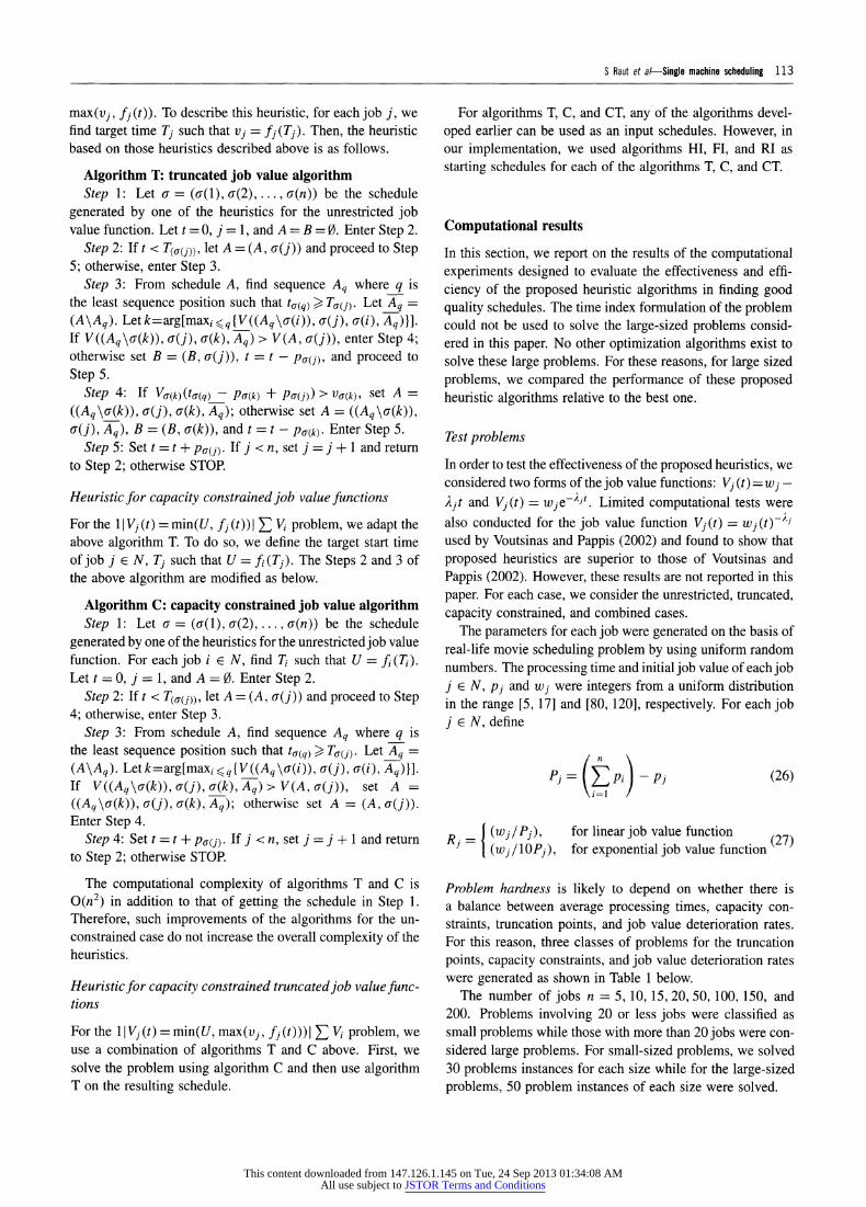
max(vj, fj (t)). To describe this heuristic, for each job j, we find target time Tj such that vj = fj (Tj). Then, the heuristic based on those heuristics described above is as follows.

Algorithm T: truncated job value algorithm Step 1: Let a = (a(1), a(2),..., a(n)) be the schedule

generated by one of the heuristics for the unrestricted job value function. Let t = 0, j = 1, and A = B = 0. Enter Step 2.

Step 2: If t < T(w(j)), let A = (A, a(j)) and proceed to Step 5; otherwise, enter Step 3.

Step 3: From schedule A, find sequence Aq where q is the least sequence position such that

ta(q) ? Ta(j). Let Aq =

(A\Aq). Let k=arg[maxi <q{V((Aq\a(i)), a(j), a(i), Aq)}]. If V((Aq\a(k)), a(j), a(k), Aq)> V(A, a(j)), enter Step 4; otherwise set B = (B, a(j)), t = t - p,(j), and proceed to Step 5.

Step 4: If Va(k)(ta(q) - Pa(k) + PU(j)) > Va(k), set A =

((Aq\a(k)), a(j), a(k), Aq); otherwise set A = ((Aq\a(k)), a(j), Aq), B = (B, a(k)), and t = t - Pa(k). Enter Step 5.

Step 5: Set t = t + pa(j). If j < n, set j = j + 1 and return to Step 2; otherwise STOP.

Heuristic for capacity constrained job value functions

For the 1l Vj (t) = min(U, fj (t)) I E Vi problem, we adapt the above algorithm T. To do so, we define the target start time of job j E N, Tj such that U = fi (Tj). The Steps 2 and 3 of the above algorithm are modified as below.

Algorithm C: capacity constrained job value algorithm Step 1: Let a = (a(1), a(2), ..., a(n)) be the schedule

generated by one of the heuristics for the unrestricted job value function. For each job i E N, find Ti such that U = fi(Ti). Let t = 0, j = 1, and A = 0. Enter Step 2.

Step 2: If t < T(,(j)), let A = (A, a(j)) and proceed to Step 4; otherwise, enter Step 3.

Step 3: From schedule A, find sequence Aq where q is the least sequence position such that t(q) ~ T,(j). Let Aq =

(A\Aq). Let k=arg[maxi q {V((Aq\a(i)), a(j), a(i), Aq)}]. If V((Aq\a(k)), a(j), a(k), Aq)> V(A, a(j)), set A =

((Aq\a(k)), a(j), a(k), Aq); otherwise set A = (A, a(j)). Enter Step 4.

Step 4: Set t = t + pa(j). If j < n, set j = j + 1 and return to Step 2; otherwise STOP.

The computational complexity of algorithms T and C is O(n2) in addition to that of getting the schedule in Step 1. Therefore, such improvements of the algorithms for the unconstrained case do not increase the overall complexity of the heuristics.

Heuristic for capacity constrained truncated job value functions

For the II Vj (t) = min(U, max(vj, f1 (t))) I Vi problem, we use a combination of algorithms T and C above. First, we solve the problem using algorithm C and then use algorithm T on the resulting schedule.

For algorithms T, C, and CT, any of the algorithms developed earlier can be used as an input schedules. However, in our implementation, we used algorithms HI, FI, and RI as starting schedules for each of the algorithms T, C, and CT.

Computational results

In this section, we report on the results of the computational experiments designed to evaluate the effectiveness and effi- ciency of the proposed heuristic algorithms in finding good quality schedules. The time index formulation of the problem could not be used to solve the large-sized problems considered in this paper. No other optimization algorithms exist to solve these large problems. For these reasons, for large sized problems, we compared the performance of these proposed heuristic algorithms relative to the best one.

Test problems

In order to test the effectiveness of the proposed heuristics, we considered two forms of the job value functions: Vj (t)= wj- Xjt and Vj(t) = wje-2Jt. Limited computational tests were also conducted for the job value function Vj(t) = wj(t)-?j used by Voutsinas and Pappis (2002) and found to show that proposed heuristics are superior to those of Voutsinas and Pappis (2002). However, these results are not reported in this paper. For each case, we consider the unrestricted, truncated, capacity constrained, and combined cases.

The parameters for each job were generated on the basis of real-life movie scheduling problem by using uniform random numbers. The processing time and initial job value of each job j e N, pj and wj were integers from a uniform distribution in the range [5, 17] and [80, 120], respectively. For each job j e N, define

-j = pi -p(26)

R (wj / Pj), for linear job value function (27) 1 (wj/lOPj), for exponential job value function

Problem hardness is likely to depend on whether there is a balance between average processing times, capacity constraints, truncation points, and job value deterioration rates. For this reason, three classes of problems for the truncation points, capacity constraints, and job value deterioration rates were generated as shown in Table 1 below.

The number of jobs n = 5, 10, 15, 20, 50, 100, 150, and 200. Problems involving 20 or less jobs were classified as small problems while those with more than 20 jobs were considered large problems. For small-sized problems, we solved 30 problems instances for each size while for the large-sized problems, 50 problem instances of each size were solved.




Table 1 Levels of the job value functions

Level Truncation Capacity Deterioration rate

Low Tj e {0.1 * Pj,...,0.25 * Pj} Uj e {50,...,70} j• E {0.01 * Rj ... 0.1 * Rj}

Medium Tj e {0.26 * Pj, ... 0.50 * Pj Uj e {60,...,801} . E 10.05 Rj, ..., 0.50 * Rj}

High Tj E {0.51 Pj,.. 0.75* P} Uj {70,...90)} 1jE {0.1*Rj .... 0.75* Rj}

Table 2 Average optimality gap of the proposed algorithms for small problems

n H HI HIT* F FI FIT* R RI RIT V VI VIT*

Linear 5 1.02 0.25 0.05 0.09 0.02 0.00 0.86 0.19 0.03 1.79 0.25 0.05 truncated 10 1.04 0.39 0.17 0.06 0.01 0.01 0.89 0.23 0.09 2.24 0.24 0.10

15 1.08 0.50 0.21 0.06 0.02 0.02 0.85 0.28 0.09 2.12 0.28 0.10 20 1.13 0.56 0.25 0.08 0.03 0.03 0.94 0.28 0.11 2.17 0.29 0.13

Average 1.07 0.42 0.17 0.07 0.02 0.02 0.88 0.24 0.08 2.08 0.27 0.10

Capacitated 5 2.65 1.14 0.94 0.97 0.81 0.80 2.86 1.04 0.94 3.67 1.18 0.97 linear 10 2.68 1.18 0.96 0.94 0.78 0.76 2.55 1.08 0.89 3.17 1.13 0.93

15 2.97 1.11 0.90 0.91 0.80 0.78 2.51 1.10 0.88 3.49 1.11 0.90 20 2.89 1.26 0.99 0.98 0.85 0.82 2.44 1.27 0.97 3.04 1.21 0.96

Average 2.80 1.17 0.95 0.95 0.81 0.79 2.59 1.12 0.92 3.34 1.16 0.94

Capacitated 5 1.18 0.98 0.85 0.84 0.83 0.83 1.26 1.02 0.87 1.49 0.95 0.84 linear 10 1.17 1.06 0.80 0.78 0.76 0.75 1.21 1.03 0.78 1.31 0.99 0.79 truncated 15 1.25 1.12 0.81 0.81 0.77 0.77 1.24 1.07 0.80 1.52 1.03 0.80

20 1.22 1.13 0.85 0.84 0.82 0.81 1.22 1.07 0.84 1.35 1.03 0.84 Average 1.21 1.07 0.83 0.82 0.79 0.79 1.23 1.05 0.82 1.42 1.00 0.82

Exponential 5 5.46 1.64 1.37 0.38 8.18 0.60 13.17 0.60 10 6.53 1.46 1.84 0.72 8.06 0.25 17.79 0.27 15 5.83 1.09 1.72 0.58 7.38 0.22 18.41 0.21 20 7.41 1.26 2.29 0.63 7.72 0.12 19.34 0.15

Average 6.31 1.36 1.80 0.58 7.84 0.30 17.18 0.31

Exponential 5 4.95 2.14 1.04 0.61 0.17 0.07 4.37 0.94 0.28 8.42 1.12 0.32 truncated 10 5.29 2.81 1.56 0.60 0.20 0.18 3.97 0.89 0.28 11.15 0.95 0.31

15 4.90 2.72 1.28 0.54 0.16 0.15 3.25 0.91 0.28 11.19 0.95 0.27 20 5.88 2.99 1.57 0.66 0.18 0.17 3.59 0.86 0.26 11.96 0.96 0.26

Average 5.26 2.66 1.36 0.60 0.18 0.14 3.80 0.90 0.27 10.68 0.99 0.29

Capacitated 5 7.58 2.26 1.34 2.27 0.75 0.66 8.21 1.39 0.97 15.40 1.26 0.91 exponential 10 9.58 3.57 1.60 3.40 1.54 0.98 10.74 2.81 1.30 18.87 2.47 1.33

15 9.07 3.81 1.63 3.73 1.96 1.10 10.10 2.97 1.28 19.26 2.41 1.21 20 10.69 4.81 1.95 4.56 2.54 1.27 11.05 3.75 1.51 19.71 3.08 1.35

Average 9.23 3.61 1.63 3.49 1.70 1.00 10.02 2.73 1.26 18.31 2.31 1.20

Capacitated 5 5.89 2.62 0.82 0.99 0.64 0.58 4.79 1.44 0.66 9.25 1.53 0.67 exponential 10 6.84 4.31 1.19 1.19 0.75 0.61 5.43 2.33 0.87 11.19 2.45 0.94 truncated 15 6.65 4.66 1.06 1.34 0.79 0.64 4.98 2.48 0.90 11.22 2.54 0.89

20 7.66 5.52 1.20 1.68 1.10 0.77 5.62 3.03 1.00 11.60 3.08 0.99 Average 6.76 4.28 1.07 1.30 0.82 0.65 5.21 2.32 0.86 10.81 2.40 0.87

*Depending on the specific case being considered, T represents the use of algorithm T, C, or TC.

Algorithm effectiveness for small problems

Each problem instance was formulated an integer program and was solved to optimality by CPLEX 7.0 in Solaris 5.8 Environment. The average CPU time for these small sizes of problems on CPLEX 7.0 in Solaris 5.8 Environment was

approximately 30 s. Each greedy and adjacent pairwise interchange algorithms were used for each problem instance re-

gardless of the nature of the job value function. In addition, each problem instance was solved using each of the algorithms applicable to the specific job value function being considered. For example, for the truncated and capacity constrained cases, algorithms T and C were used, respectively. Similarly for the combined case, both algorithms T and C were used. However, to keep the tables manageable, algorithms T, C, or TC are represented by T only. However, the designation




Table 3 Maximum optimality gap of the proposed algorithms for small problems

n H HI HIT* F FI FIT* R RI RIT* V VI VIT*


15 5.35 3.26 1.92 0.40 0.34 0.34 3.61 1.54 1.13 9.88 1.56 1.08 20 4.36 3.00 2.17 0.45 0.37 0.37 3.85 1.76 1.31 11.47 1.76 1.31

Overall 12.10 5.32 2.81 1.71 0.69 0.51 8.92 3.78 1.72 15.34 4.72 2.54


15 13.65 5.36 3.02 2.97 1.84 1.84 10.19 5.46 2.17 15.78 5.52 2.80 20 11.40 5.59 3.36 3.13 2.32 1.86 8.89 7.33 3.92 13.35 4.85 2.58

Overall 13.65 12.29 7.19 4.36 3.30 2.68 13.88 7.33 7.19 19.84 12.29 8.40


20 10.22 9.68 5.21 5.33 5.25 4.71 8.84 7.16 5.32 12.86 6.34 4.59 Overall 10.22 9.68 5.21 5.33 5.25 4.71 8.84 7.16 5.32 14.82 6.34 4.59

Exponential 5 23.95 22.83 14.05 13.25 35.50 22.83 38.29 22.83 10 16.98 11.80 8.41 5.79 25.43 5.58 48.57 4.78 15 12.65 5.86 7.22 5.27 23.61 3.13 38.03 2.18 20 12.38 3.81 4.32 2.35 11.67 0.59 31.94 0.84

Overall 23.95 22.83 14.05 13.25 35.50 22.83 48.57 22.83


15 13.63 9.42 7.69 3.99 2.60 2.60 9.46 4.39 2.82 36.07 4.39 2.82 20 18.56 10.05 7.86 4.30 3.00 3.00 9.07 3.53 1.77 42.47 3.53 1.27

Overall 26.85 23.56 22.24 14.30 14.30 3.83 26.85 24.19 22.24 42.47 24.19 22.24


15 20.46 16.12 6.63 11.14 9.76 5.28 32.76 18.22 7.42 39.70 9.23 6.09 20 22.09 17.42 7.45 14.70 9.60 5.71 32.66 13.71 6.85 46.31 13.13 5.66

Overall 31.08 17.96 10.64 17.10 14.55 6.39 34.67 19.11 13.26 50.57 14.55 9.24


20 22.16 17.48 5.64 9.17 6.89 3.52 17.64 12.89 4.39 43.32 13.12 5.11 Overall 30.70 23.88 8.59 14.94 7.70 6.17 33.18 22.86 6.94 48.07 22.86 7.02


of specific cases being considered makes the context quite clear.

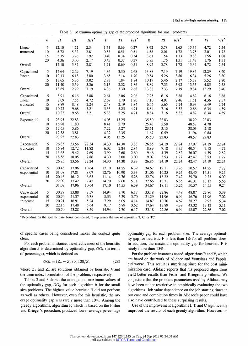
For each problem instance, the effectiveness of the heuristic algorithm h is determined by optimality gap, OGh (in terms of percentage), which is defined as

OGh = (Zo - Zh) X 100/Zo (28)

where Zh and Zo are solutions obtained by heuristic h and the time-index formulation of the problem, respectively.

Tables 2 and 3 depict the average and maximum values of the optimality gap, OGh for each algorithm h for the small size problems. The highest value heuristic H did not perform as well as others. However, even for this heuristic, the average optimality gap was rarely more than 10%. Among the greedy algorithms, algorithm F, which is based on the Fisher and Krieger's procedure, produced lower average percentage

optimality gap for each problem size. The average optimality gap for heuristic F is less than 1% for all problem sizes. In addition, the maximum optimality gap for heuristic F is rarely more than 15%.

For the problem instances tested, algorithms R and V, which are based on the work of Alidaee and Voutsinas and Pappis, did worse. This result is surprising since for the cost mini- mization case, Alidaee reports that his proposed algorithms yield better results than Fisher and Krieger algorithms. We conjecture that the problem parameters used by Alidaee may have been rather restrictive in empirically evaluating the two algorithms. Job value dependence on the job starting times in our case and completion times in Alidaee's paper could have also have contributed to these surprising results.

Use of the improvement algorithms I, T, and C significantly improved the results of each greedy algorithm. However, on




Table 4 Average optimality gap of the proposed algorithms for large problems

n H HI HIf F FI FIT* R RI RIT* V VI VIT*


150 1.07 0.55 0.28 0.05 0.00 0.00 0.87 0.30 0.11 2.05 0.32 0.12 200 1.07 0.56 0.28 0.05 0.00 0.00 0.86 0.30 0.11 2.06 0.32 0.12

Average 1.06 0.51 0.25 0.05 0.01 0.00 0.87 0.28 0.10 2.05 0.30 0.12


150 2.42 0.99 0.34 0.19 0.07 0.00 1.87 0.84 0.25 2.49 0.83 0.26 200 2.52 1.07 0.35 0.21 0.09 0.00 1.96 0.94 0.26 2.58 0.93 0.28

Average 2.40 0.89 0.31 0.19 0.07 0.00 1.86 0.78 0.23 2.48 0.77 0.25


200 0.62 0.55 0.07 0.06 0.03 0.00 0.61 0.48 0.05 0.71 0.44 0.05 Average 0.56 0.48 0.06 0.05 0.02 0.00 0.54 0.42 0.05 0.66 0.37 0.04

Exponential 50 7.42 0.99 2.45 0.69 7.04 0.07 19.75 0.05 100 8.03 1.04 2.63 0.76 7.04 0.06 19.42 0.03 150 7.99 1.13 2.68 0.79 6.71 0.01 19.77 0.03 200 8.22 1.17 2.77 0.86 6.85 0.03 19.91 0.03

Average 7.92 1.08 2.63 0.78 6.91 0.04 19.71 0.03


150 6.10 3.60 1.90 0.72 0.19 0.19 3.15 0.81 0.08 11.82 0.87 0.11 200 6.24 3.70 1.98 0.74 0.21 0.21 3.18 0.84 0.07 11.93 0.91 0.10

Average 6.04 3.48 1.83 0.71 0.18 0.18 3.18 0.82 0.09 11.83 0.89 0.12


150 10.58 4.51 0.88 4.44 2.25 0.22 9.80 4.24 0.60 19.01 3.14 0.37 200 10.62 4.50 0.84 4.35 2.23 0.18 9.91 4.23 0.61 19.17 3.15 0.38

Average 10.55 4.33 0.87 4.32 2.12 0.24 9.97 3.97 0.59 19.01 2.95 0.39


200 7.63 5.80 0.50 1.52 0.87 0.00 5.00 3.06 0.28 11.09 3.11 0.29 Average 7.49 5.62 0.50 1.43 0.76 0.02 4.98 2.91 0.27 10.94 2.96 0.28


the average, algorithm FI leads to lower percentage optimality gaps than algorithms HI, RI, and VI. The use of algorithms T and C for the truncated and capacity constrained problems dramatically improves the performance of algorithms HI, FI, RI, and VI. In fact, use of algorithms I, T, and C reduces the average and maximum gaps to less than 1 and 9% for all

algorithms. As the problem size increases, the performance of each

heuristic decreases, but not significantly. Further, while not shown in the tables, heuristics performed worse on problems with low or high levels of deterioration rate and high level of truncation.

Algorithm effectiveness for large problems

Each problem instance (n = 50, 100, 150, and 200 jobs) was solved using each of the algorithms applicable to the specific

job value function being considered. Further, each greedy and

adjacent pairwise interchange algorithms were used for each

problem instance regardless of the nature of the job value function.

For large job size problems, the average CPU times on CPLEX 7.0 in Solaris 5.8 Environment were greater than 2 h. Therefore, we used the best value of the objective function obtained by any of the heuristic in the same class (like the H, F, R, and V) as a surrogate of an optimal solution value. Therefore, for each set of 50 large problems instances, we have calculated the optimality gap, OGh for each heuristic h as follows:

OGh = (Zc - Zh) x 100/Zc (29)

where Zc is the best solution among heuristics from class c.




Table 5 Maximum optimality gap of the proposed algorithms for large problems

n H HI HIT* F FI FIT* R RI RIT* V VI VI7T


150 3.86 2.52 1.83 0.21 0.10 0.09 2.81 1.10 0.58 7.33 1.11 0.71 200 3.87 2.30 1.56 0.22 0.02 0.02 2.75 0.94 0.49 7.02 1.06 0.60

Overall 4.37 2.74 1.83 0.27 0.15 0.15 3.20 1.34 0.75 8.98 1.43 0.77


150 9.54 4.78 2.32 1.94 0.93 0.00 7.47 4.42 1.97 10.96 4.13 2.04 200 9.39 5.00 2.35 1.82 1.04 0.00 7.42 4.32 1.54 10.49 4.92 1.75

Overall 10.72 5.03 2.45 2.18 1.14 0.01 8.30 4.84 2.49 12.58 4.98 3.22


200 6.38 5.70 1.26 1.38 0.89 0.01 5.49 4.11 0.92 7.26 4.03 0.90 Overall 6.82 6.07 1.79 1.64 1.00 0.16 5.98 4.50 1.46 8.68 4.53 1.28

Exponential 50 10.48 3.44 4.15 1.80 13.68 0.83 25.35 0.33 100 10.37 2.57 3.86 1.53 10.76 0.57 23.52 0.20 150 10.52 2.65 3.89 1.74 10.76 0.57 23.52 0.20 200 10.11 2.13 3.68 1.80 9.64 0.35 24.01 0.16

Overall 10.52 3.44 4.15 1.80 13.68 0.83 25.35 0.33


150 13.49 9.43 5.79 3.88 1.92 1.92 6.13 1.95 0.65 29.05 2.03 0.64 200 13.42 11.08 6.45 3.67 1.44 1.44 6.08 1.98 0.53 30.61 2.02 0.59

Overall 14.08 11.08 6.45 4.45 1.92 1.92 7.50 2.83 1.87 32.71 2.83 0.82


150 18.68 11.82 5.57 10.08 7.05 2.17 22.48 13.74 3.39 34.13 8.57 2.31 200 17.64 11.48 4.25 9.97 6.45 1.40 22.68 15.98 4.37 35.27 8.18 2.05

Overall 21.05 14.42 6.72 12.37 9.22 3.68 26.70 15.98 5.59 38.07 9.27 4.12


200 19.76 16.45 2.62 6.95 4.30 0.40 11.72 8.56 1.49 31.76 8.74 1.45 Overall 21.81 17.03 3.73 7.09 5.24 1.28 16.93 10.43 2.28 34.12 10.48 2.83


Tables 4 and 5 show the average and maximum values of the optimality gap, OGh for each algorithm h for the large size problems. The results in Table 4 confirm the conclusions for the small problems. Greedy algorithms based on the Fisher and Krieger's procedure, like algorithm F produced lower average percentage optimality gap for each problem size, the average optimality gap being 4.5% or less. Greedy algorithms based on the work of Alidaee and Voutsinas and Pappis did worse.

Use of the improvement algorithm I significantly improved the results of each greedy algorithm, bringing the average optimality gap to less than 1% for heuristics FI, FIT(C), RI, RIT(C), and VIT(C). However, on the average, algorithm FI leads to lower percentage optimality gaps than algorithms HI, RI, and VI. Further, compared to the results for small problems, the neighbourhood improvement algorithm I produced significantly more improvements for large problems.

The use of algorithms T and C for the truncated and capacity constrained problems dramatically improves the performance of algorithms HI, FI, RI, and VI. The maximum optimality gap values in Table 5 show a similar pattern as those for small problems in Table 3. While not shown in Tables 4 and 5, each heuristic performed worse on problems with low or high deterioration rates and low and high capacity restrictions.

From the above computational results, algorithms based on the piecemeal linear approximation of the job value functions suggested by Fisher and Krieger generate the best schedules for the single machine problems with deteriorating job value functions. Algorithm V based on the work of Voutsinas and Pappis consistently performed worse producing optimality gaps greater than heuristic H. However, even for algorithm V, used of proposed improvement heuristics significantly improved its effectiveness.




Conclusions

This paper considered the problem of scheduling a given number of movies in a theatre to maximize total profit. The problem is formulated as one of scheduling jobs on a single machine where the job value deteriorate with its start time and

designated by l Vj(t)| max Vj. In view of several practical applications of the problems, different operating configu- rations, like the limitations on the job values due to the machine capacity constraint were also considered. In addition, this paper analyses cases where the job values may stop de-

teriorating after a specified starting time.

Except for a some special cases, the II Vj (t)l max ~ Vj problem was shown to be unary NP-hard where the job deterioration function is Vj (t) is a non-increasing function of the starting time of job j. In view of the NP-hard nature of the problem, several heuristic algorithms are developed to find optimal or near optimal schedules for various cases of the Il Vj (t)I max E V1 problem. Computational results over a

large number of problems show that the proposed algorithms generated near-optimal solutions for a large number of problem instances. Among the heuristics tested, heuristic F produced the best results while algorithm V produced the worst results. Further, the use of the adjacent pair-wise interchange algorithm I was found to substantially improve the quality of the solutions obtained by any of the proposed greedy algorithms. Use of algorithms T and C could further improve the results.

While we considered the single machine scheduling problem where the job value deterioration depends on the job starting times, we note that our results and proposed heuristic

algorithms can easily be adapted to the problems where the

job value deterioration depends on the job completion times.

Except for some minor changes in the details of the proofs, all complexity results are valid for the I I Vj (Cj)l max 1 Vj problem where Cj is the completion time of job j. Similarly, for the proposed heuristics, equivalent job selection criteria can easily be described for the Ii Vj (Cj) I max E Vj problem.

The development of various heuristic algorithms in this

paper also results in some fruitful directions for future research. First, it would be helpful to develop tight bounds and some dominance conditions to develop an effective branch and bound algorithm for the II Vj (t)l max E Vj problem. Second, the proposed heuristics can be modified to obtain improved solutions.

One way to do this is to use combinations of the proposed heuristics. For example, algorithms F, H, and R could be used in combination to improve the solution value. Third, it would be interesting to develop heuristics for the II Vj (t) I max C Vj problem with specified worse-case performance bounds. Fourth, it would be interesting and useful to develop and evaluate various local search heuristics such as tabu search and genetic algorithms. Finally, extension of the results to schedule movies in a multiplex theatre where several movie

screens are available to schedule multiple movies at the same time would enhance the practical utility of scheduling theory. Thus, more research is necessary in the area of scheduling on non-manufacturing sector.

Acknowledgements- Constructive comments from two anonymous re- viewers improved the presentation of this paper. This research was par- tially supported by a financial grant to Sanjeev Swami under the Young Scientist Scheme of the Department of Science and Technology, Govern- ment of India.

References

Alidaee B (1991). Single machine scheduling with nonlinear cost functions. Comput Opns Res 18: 317-332.

Alidaee B (1993). Numerical methods for single machine scheduling with non-linear cost functions to minimize total cost. J Opl Res Soc 44: 125-132.

Fisher ML and Krieger AM (1981).Analysis of a linearization heuristic for single-machine scheduling to maximize profit. Working Paper, Department of Decision Sciences, The Wharton School, University of Pennsylvania.

Fisher ML and Krieger AM (1984). Analysis of a linearization heuristic for single-machine scheduling to maximize profit. Math Programming 28: 218-225.

Fleischmann M et al (1997). Quantitative models for reverse logistics: a review. Eur J Opl Res 103: 1-17.

Garey MR and Johnson DS (1979). Computers and Intractability-A Guide to the Theory of NP-Completeness. Freeman: San Francisco, CA.

Lawler EL (1976). Combinatorial Optimization: Networks and Metriods. Holt, Rinehart and Winston: New York.

Lawler EL (1977). A pseudo-polynomial algorithm for sequencing jobs to minimize total tardiness. Ann Discrete Math 1: 331-342.

Lawler EL, Lenstra JK, Rinnooy Kan AHG and Shmoys DB (1993). Sequencing and scheduling: algorithm and complexity. In: Graves SC, Rinnooy Kan AHG and Zipkin PH (eds). Handbooks in Operations Research and Management Science, Volume 4: Logistics of Production and Inventory. North-Holland, Amsterdam, pp 445-522.

Lenstra JK, Rinnooy Kan AHG and Brucker P (1977). Complexity of machine scheduling problems. Ann Discrete Math 1: 343-362.

Smith WE (1956). Various optimizers for single-stage production. Naval Res Logistics Quart 3: 59-66.

Sousa JP and Wolsey LA (1992). A time-index formulation of non-preemptive single machine scheduling problems. Math Programming 54: 353-367.

Swami S, Jehoshua E and Charles BW (1999). SilverScreener: a modeling approach to movie screens management. Market Sci (Special Issue on Managerial Decision Making) 18: 352-372.

Voutsinas TG and Pappis CP (2002). Scheduling jobs with values exponentially deteriorating over time. Int J Product Econ 79: 163 -169.

Xia Y and Tse D (2000). Survey of single machine scheduling with application to web object transmission. Department of Electrical Engineering and Computer Science, University of California: Berkeley.

Received February 2006;

accepted June 2006



Documents

Single Machine Scheduling with Time Deteriorating Job Values