Size-related premiums

Size-related premiums

THIAGO DE OLIVEIRA SOUZA∗

Current Version: June 27, 2017First Draft: November 18, 2015

ABSTRACT

The size premium only exists in high market price of risk states because ranking stocks by

size is only equivalent to ranking them by risk if the differences in risk premiums overcome

differences in expected cash flows among them. In these states, the size premium spans

the value premium. Consequently, there is no particular risk associated with the book-to-

market characteristic of the stocks, which is simply a version of size, scaled by a proxy for

expected cash flows. This contradicts the characteristic based explanations of the value

premium, including the ones assuming costly adjustments to installed capital.

JEL Classification: G11, G12, G14.

Keywords: Size premium, Value premium, Risk, Conditional, Adjustment costs.

∗Department of Business and Economics, University of Southern Denmark, Campusvej 55, 5230Odense M, Denmark. Email: [email protected]. I would like to thank Stefano Giglio, John Cochrane,Paulo Maio, Jonathan Berk, Christian Flor, Linda Larsen, Francisco Gomes, Jaime de Jesus, and theparticipants in the World Finance Conference 2016.

Several empirical studies describe stocks in terms of some characteristics that are sup-

posedly related to risk premiums.1 Two of these characteristics stand out following Fama

and French (1996): One is the market value of equity in the firm (size). The second is

the book-to-market ratio (BM), which is size divided by the book value of equity (BE).

These characteristics have been linked to the size and to the value risk premiums, respec-

tively, often overlooking how volatile the characteristics are relative to the frequency at

which we expect the risk of the stocks to vary. For example, the link between risk and a

price-related characteristic cannot be constant unless the risk of the stocks change every

time their prices change. Thus, it can be problematic to determine this link without

understanding the mechanism behind it.

The apparent association between the BM characteristic and the risk of the stocks,

for example, gives empirical support to the idea that firms become riskier when they

increase their tangible assets. A prolific literature on adjustment costs is broadly based

on this assumption:2 Tangible assets in place (and their variants, such as fixed operating

costs) are claimed to be risky because reverting an investment decision is costly once the

physical capital is installed and also because this tends to happen in bad states of the

economy. Considering the BE as a proxy for installed capital connects this theory to the

BM characteristic of the firms. Therefore, observing a positive relation between the BM

and the risk premiums in the data confirms the ideas in these models.

This paper has three goals. The first is to establish the link between the risk of

the stocks and their size-related characteristics as a function of the market conditions.

The second is to understand which risks are associated with the size and with the value

characteristics. The third is to investigate whether the BE carries any risk information

in the way predicted by the literature on costly adjustment to the capital stock.

1See, for example, Harvey, Liu, and Zhu (2016).2The related literature goes back at least to Berk, Green, and Naik (1999) and includes, for example,

Carlson, Fisher, and Giammarino (2004), Zhang (2005), Cooper (2006), Novy-Marx (2011), Obreja(2013), Ai, Croce, and Li (2013), Choi (2013), and Kogan and Papanikolaou (2013).

2

I construct a theoretical framework in which the most restrictive assumption is the

one of a time-varying market price of risk.3 This implies that risk and size are only

related when the market price of risk is high, as the empirical evidence in Souza (2017)

suggests. The intuition is similar to Berk (1995): Given two stocks with the same expected

cash flows, the riskier stock has a higher required return and therefore a lower market

value. So this relates small stocks to large risk premiums. But for firms with different

expected cash flows, the size ranking only aligns with the risk ranking if the difference in

required premiums is sufficiently large to overcome the difference in expected cash flows

and dominate the size ranking. Hence, there must be a threshold for the market price of

risk above which the size and the risk rankings become aligned in general.

Establishing the link between risk and the BM characteristic is less straightforward

because it also involves determining the risks associated with the BE. In this respect,

there are two possibilities: The BE is either a proxy for expected cash flows (Berk, 1995),

or the BE is related to some risks, which could be real frictions on the firms’ investments

(Zhang, 2005), for example. I test these two hypotheses.

In summary, if the BE is related to some specific risks, the value ranking should always

capture these risks while the size ranking should not, regardless of the prevailing market

price of risk. Alternatively, the BE may simply help aligning the value ranking with the

risk ranking by controlling for the cross-sectional variation in expected cash flows (Berk,

1995). Given that controlling for cash flows is unnecessary when the market price of risk

is high (because the size ranking already aligns with the risk ranking), the value ranking

should only capture additional risks compared to the size ranking when the market price

of risk is low under this second hypothesis.

3There is a myriad of models based on different assumptions that generate time variation in themarket price of risk. Examples of these models include Campbell and Cochrane (1999), Shiller (2014),Rietz (1988), Barro (2006), Piazzesi, Schneider, and Tuzel (2007), Brunnermeier (2009), Hansen andSargent (2001), Epstein and Zin (1989), Bansal and Yaron (2004), Bansal, Kiku, and Yaron (2012),Constantinides and Duffie (1996), and Garleanu and Panageas (2015).

3

The empirical tests reveal the absence of any premium associated with value that is not

also (potentially) associated with size: The size premium spans the value premium in high

market price of risk states.4 There is no excess return associated with the HML portfolio

of Fama and French (1996) after controlling for its exposure to the SMB portfolio, and

the correlation between the returns on the two portfolios is highly significant in these

states. The difference is that the mean return on the HML portfolio is also positive in

low market price of risk states. In these states, the mean return on the SMB portfolio is

zero, there is zero correlation between the return on the two portfolios, and the positive

premium associated with the HML portfolio is unexplained by the return on the SMB

portfolio.

Finally, the conclusion from the findings above is that the BE and other scaling

variables are proxies for expected cash flows and are unrelated to the risk of the stocks.

In particular, I find no empirical support for the idea that the risks associated with

adjustments to installed capital are priced in equilibrium.

In fact, this paper is not the first to reject the hypothesis that the BM characteristic

is responsible for the value premium in favour of a risk based explanation. In a different

context, Davis, Fama, and French (2000), replying to Daniel and Titman (1997), also

reject the hypothesis that differences in the BM characteristic among the stocks generate

the value premium. More recently, Chordia, Goyal, and Shanken (2015) also contribute

to this literature.

This paper is also part of a long literature on the relation between stock characteristics

and premiums in cross section.5 Within this literature, its most important contribution

4I use the state variables in Souza (2017) as proxies for the market price of risk: The median BMof all CRSP stocks (MBM), the value weighted BM of all CRSP stocks (VBM), the Dow Jones’ BM ofPontiff and Schall (1998) (DJBM), the earnings-price ratio of all S&P Composite stocks (EP), the termspread (TMS), the default spread (DFY) and the Treasury bill rate (TBL).

5An incomplete list includes Banz (1981), Jegadeesh and Titman (1993), Fama and French (1996,2015, 2016), Li, Livdan, and Zhang (2009), Novy-Marx (2013), Hou, Xue, and Zhang (2015), Harveyet al. (2016), Green, Hand, and Zhang (2017), and Light, Maslov, and Rytchkov (2017).

4

is to show that the value and the size premiums do not correspond to two independent

risk dimensions as previously assumed. In addition, the paper provides a theoretical

explanation for the conditional size premium that is empirically documented in Souza

(2017).

I. Theoretical framework

Let ζ = (ζt) be the unique stochastic discount factor (SDF) that follows the continuous-

time stochastic process

dζt = −ζt[rft dt+ λt dz1t], (1)

where dz1t is a one-dimensional standard Brownian motion and the stochastic processes,

rft and λt, represent the risk free rate and the market price of risk process at time t,

respectively.

Let Pi = (Pit) be the price process of portfolio i, such that

dPit = Pit[µit dt+ σit dz1t + σ̃>it dzt], (2)

where µit and σit are one-dimensional stochastic processes, dzt is a multi-dimensional

standard Brownian motion independent of dz1t, σ̃it is a multi-dimensional stochastic

process, and > is the transposition sign. µit and σit represent, respectively, the expected

returns and the sensitivity of the returns on the portfolio to the exogenous (priced) shocks

to the economy. So σit gives the effective risk of the portfolio. σ̃it represents the unpriced

return volatility of the portfolio (the sensitivity of the returns on the portfolio to the

exogenous unpriced shocks). Without intermediate dividends, the expected excess rate

of return on the portfolio is

µit − rft = σitλt. (3)

5

So the overall market price of risk, λt, and the risk of the portfolio, σit, combined

determine the expected returns on the portfolio at time t. In particular, by construction

of the SMB portfolio and considering Eq. (3), we have

σsmb,t = σsmall,t − σbig,t, (4)

µsmb,t = σsmb,tλt, (5)

where σsmall,t and σbig,t are, respectively, the risks of the portfolios of small stocks and big

stocks, σit in Eq. (2), and µsmb,t is the expected return on the SMB portfolio at time t.

Equivalently, for the HML portfolio we have

σhml,t = σvalue,t − σgrowth,t, (6)

µhml,t = σhml,tλt, (7)

where σvalue,t and σgrowth,t are, respectively, the risks of the portfolios of value stocks and

growth stocks at time t, and µhml,t is the expected return on the HML portfolio at time t.

A. Modelling the risk of the size-related portfolios

For tractability, assume that the risk-free rate and the market price of risk are constant

between time t and time T . So the SDF follows a one-dimensional geometric Brownian

motion process,

dζt = −ζt[rf dt+ λt dzt], (8)

where the constants λt and rf are, respectively, the market price of risk and risk free rate

prevailing from time t to time T .

As in Eq. (2), let Pi = (Pit) be the price process of the equity in the firm i. The

firm makes only a final lump sum dividend payment, Di,T , at time T , which is modelled

6

through xi,t = Et[Di,T ] following the process

dxi,t = xi,t[0 dt+ σit dz1t + σ̃>

itdzt]

], (9)

where σit is a (one-dimensional) constant and σ̃it is a (multi-dimensional) constant. Under

these conditions, the time t value of the payoff Di,T is

Pit = Et

[Di,T

ζTζt

]= Et[Di,T ]e−(rf+σitλt)(T−t), (10)

which depends positively on the expected payoff, Et[Di,T ], and negatively on the risk of

the payoff, σit, and on the market price of risk, λt, (apart from the risk free rate, rf , and

the time interval, T − t).

A.1. The size ranking

Eq. (10) summarizes the framework in Berk (1995): Given two firms with the same

expected cash flows, the riskiest one, with the largest σit, has the lowest market value,

Pit. Therefore, there is an association between a price ranking, based on Pit, and a risk

ranking, based on σit.6 However, the price ranking is only imperfectly related to the risk

ranking because the price also depends on the expected cash flows, Et[Di,T ].

As a consequence from Eq. (10), there must be a minimum market price of risk, λ∗, so

that the price ranking and the risk ranking align. Intuitively, the risk premium must be

large enough to overcome differences in expected cash flows among the firms, so that risk

is the determinant of the differences in price for a large number of stocks. This translates

into the first rejectable prediction of the model:

Hypothesis 1 (H1): The size premium is positive if and only if the market price of risk is

6Considering that the market portfolio is not on the mean-variance frontier would, thus, explain theresidual CAPM excess return associated with size.

7

above a certain threshold, λt ≥ λ∗, and is zero otherwise.

In terms of Eq. (4) and Eq. (5),

σsmb,t =

0 λt < λ∗

f(λt) > 0 λt ≥ λ∗=⇒ µsmb,t =

0 λt < λ∗

f(λt)λt > 0 λt ≥ λ∗(11)

where f(λt) is a non decreasing function of the market price of risk, λt.

More details about the market price of risk threshold, λ∗: Consider a pair of

stocks. Stock r is riskier, with volatility term σrt, and stock s is safer, with volatility

term σst, such that

σrt > σst. (12)

The price ranking and the risk ranking are aligned for this pair of stocks if and only

if the price of the risky stock is smaller than the price of the safe stock, Pr,t < Ps,t. In

terms of the parameters in Eq. (10),

Pr,t < Ps,t ⇐⇒ λt > ln

(Et[Dr,T ]

Et[Ds,T ]

)1

(σrt − σst) (T − t)≡ λ∗, (13)

where λ∗ is actually specific to this pair of stocks, but I assume it to be the same for

other pairs of stocks to simplify the argument.

Under the assumption that risk and expected cash flows are unrelated, the probabili-

ties that a given riskier firm has either larger or smaller expected cash flows than a safer

firm are the same:

P

(Et[Dr,T ]

Et[Ds,T ]≤ 1

)= P

(Et[Dr,T ]

Et[Ds,T ]> 1

). (14)

Thus, a large portfolio of small stocks should only contain a disproportionally large

8

number of risky stocks, so that σsmall,t > σbig,t, if the market price of risk is above

the threshold in Eq. (13), λt > λ∗. Otherwise, the differences in expected cash flows

dominate the price ranking and the portfolios based on this ranking have the same risks,

σsmall,t = σbig,t.

A.2. The scaled-price rankings

Consider the same pair of stocks, but ranked by a scaled-price ratio (SP). The SP

ranking is aligned with the risk ranking if and only if the SP of the risky stock is smaller

than the SP of the safe stock,

Pr,tBr,t

<Ps,tBs,t

, (15)

where the scaling variable for firm i at time t, Bi,t, divides the market value calculated

in Eq. (10) for each stock. In terms of the parameters, the equivalent of Eq. (13) is now

Pr,tBr,t

<Ps,tBs,t

⇐⇒ λt > ln

(Et[Dr,T ]

Et[Ds,T ]

Bs,t

Br,t

)1

(σrt − σst) (T − t)≡ λ∗SP . (16)

This threshold is smaller than the one in Eq. (13), λ∗SP < λ∗, as long as the scaling

variable for the risky stock is larger than the one for the safe stock, Br > Bs. In

particular, the SP ranking aligns with the risk ranking for any (positive) market price of

risk if the scaling variable is equal to the expected cash flow, Bi,t = Et[Di,T ], so we have

λt > λ∗SP = 0.

B. The BE as a proxy for expected cash flows?

Let us assume that the BE is a good proxy for the expected cash flows of at least

some of the firms and use it as a scaling variable,

Bi,t ≡ BEi,t ≈ Et[Di,T ]. (17)

9

This creates the price-to-book (PB) ratio that generates the HML portfolio.7 Under this

assumption, there is a range for the market price of risk in which the SP ranking aligns

with the risk ranking, while the price ranking does not, λ∗ > λt > λ∗SP . And depending

on how well the BE proxies for the expected cash flows, the threshold in Eq. (16) can be

zero, λ∗SP = 0.

Hence, a large portfolio of value stocks (with low PB) should contain a disproportion-

ally large number of risky stocks, so σvalue,t > σgrowth,t, even if the prevailing market price

of risk is lower than the one necessary to generate the size premium. The equivalent to

Eq. (11) for λ∗SP = 0, in terms of Eq. (6) and Eq. (7), is

σhml,t =

f(λt) > 0 λt < λ∗

f(λt) > 0 λt ≥ λ∗=⇒ µhml,t =

f(λt)λt > 0 λt < λ∗

f(λt)λt > 0 λt ≥ λ∗, (18)

which is the mathematical representation of the second testable prediction of the model:

Hypothesis 2 (H2): (Assuming that the BE is a proxy for expected cash flows). The value

premium increases with the market price of risk, being small, but still positive, even if

the market price of risk is lower than the threshold below which the size premium is zero,

λt ≤ λ∗.

C. Can the BE carry risk information about the stock?

The PB ranking can also capture some specific risks that the price ranking does

not capture if the BE is related to these specific risks. For example, the BE can be a

proxy for the installed capital in the firm which is risky according to the framework in

Zhang (2005). In order to analyse this question, I must relax the assumption that the

7The conclusions are similar for other scaling variables, such as dividends, earnings, or cash flows.This is expected because the value premium spans several other premiums associated with SP, as shownin Fama and French (1996).

10

fundamental uncertainty in the economy is modelled by the one-dimensional exogenous

shock in Eq. (1).8 Otherwise there cannot be additional risks for the scaling variables to

capture. In a multi-dimensional risk setting, the equivalents of Eq. (5) and Eq. (7) are

µsmb,t = σ>smb,tλt, (19)

µhml,t = σ>hml,tλt, (20)

where λt is the multi-dimensional market price of risk process, and σsmb,t and σhml,t are

the multi-dimensional stochastic sensitivities of the returns on the SMB and on the HML

portfolios to the (independent) exogenous priced shocks to the economy, respectively.

Now let the kth element in σsmb,t be equal to zero, while being different from zero in

σhml,t. This means that the PB ranking captures this risk, but the price ranking does

not. Consequently, it is impossible to find a constant, a, that multiplied by the risk of

the SMB portfolio, σsmb,t, gives the risk of the HML portfolio, σhml,t:

@ a ∈ R | σhml,t = aσsmb,t. (21)

And therefore, it is also impossible to represent the expected return on the HML portfolio

as a multiple of the expected return on the SMB portfolio:

@ a ∈ R | µhml,t = aσ>smb,tλt = aµsmb,t. (22)

If the BE is related to risk, then Eq. (22) should hold for every market price of risk,

λt. Alternatively, if the BE is simply a proxy for expected cash flows, Eq. (22) should

still hold when the market price of risk is low because, according to Eq. (11), the size

premium is zero in these states. But a constant, a, could exist when the market price of

8Appendix A shows the adjustments to Eq. (1) and to Eq. (2) that give the results in this section.

11

risk is high, λt > λ∗.9 Thus, testing this hypothesis empirically is equivalent to testing

whether such constant, a, exists depending on the market price of risk, λt:

Hypothesis 3 (H3): (Assuming that the BE is a proxy for expected cash flows, and is

not related to the risk of the stock). The value premium should be a multiple of the size

premium, µhml,t = aµsmb,t, if and only if the market price of risk is high, λt > λ∗.

II. Empirical section

There are three main steps in order to test the three hypotheses above. The first is to

find a proxy for the market price of risk, the second is to find the threshold above which

the size ranking aligns with the risk ranking, and the third is to finally investigate the

conditional relation between the size and the value premiums.

A. Data and variables

A.1. The market price of risk proxy

I consider the typical ICAPM state variables related to the size premium in Souza

(2017) as proxies for the market price of risk. Souza (2017) shows that these variables

forecast positive market conditions. This gives them a market price of risk interpretation.

The state variables that I calculate from the data in Kenneth French’s data library

(time span in brackets) are the median BM of all CRSP stocks (MBM, 1926–2015) and the

value weighted BM of all CRSP stocks (VBM, 1926–2015).10 The variables that I obtain

from Goyal’s website are the Dow Jones’ BM of Pontiff and Schall (1998) (DJBM, 1921–

2015), the earnings-price ratio (EP, 1871–2015), the term spread (TMS, 1920–2015), the

9In fact, the constant a only exists in general if the size and the value rankings have the same relativeexposures to the different priced shocks to the economy.

10http://mba.tuck.dartmouth.edu/pages/faculty/ken.french/data library.html.

12

default spread (DFY, 1919–2015), and the Treasury bill rate (TBL, 1920–2015).11 The

TBL actually forecasts negative market conditions. So I subtract it from one to obtain

the same market price of risk interpretation as the other variables. The values of the

state variables in year t correspond the end of June of year t.

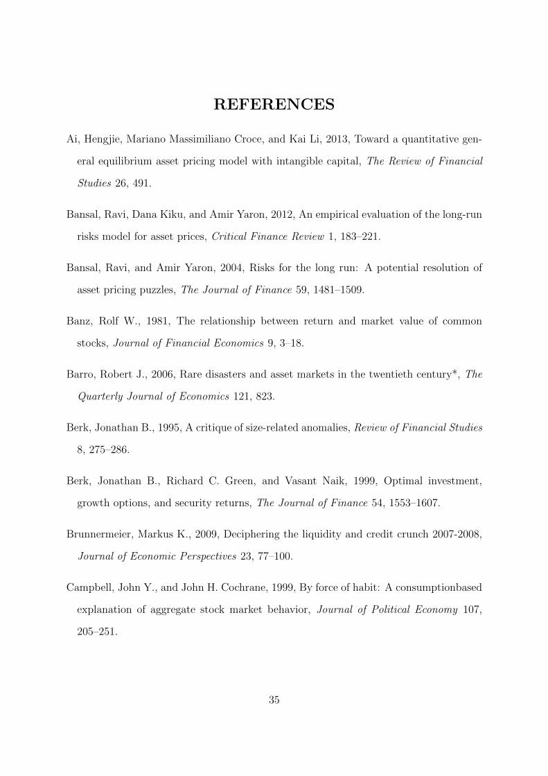
Table I presents the same summary statistics in Souza (2017) for the state variables,

assuming that they follow a first order AR process. The state variables tend to be

persistent but are stationary in line with the fact that they are essentially ratios. The

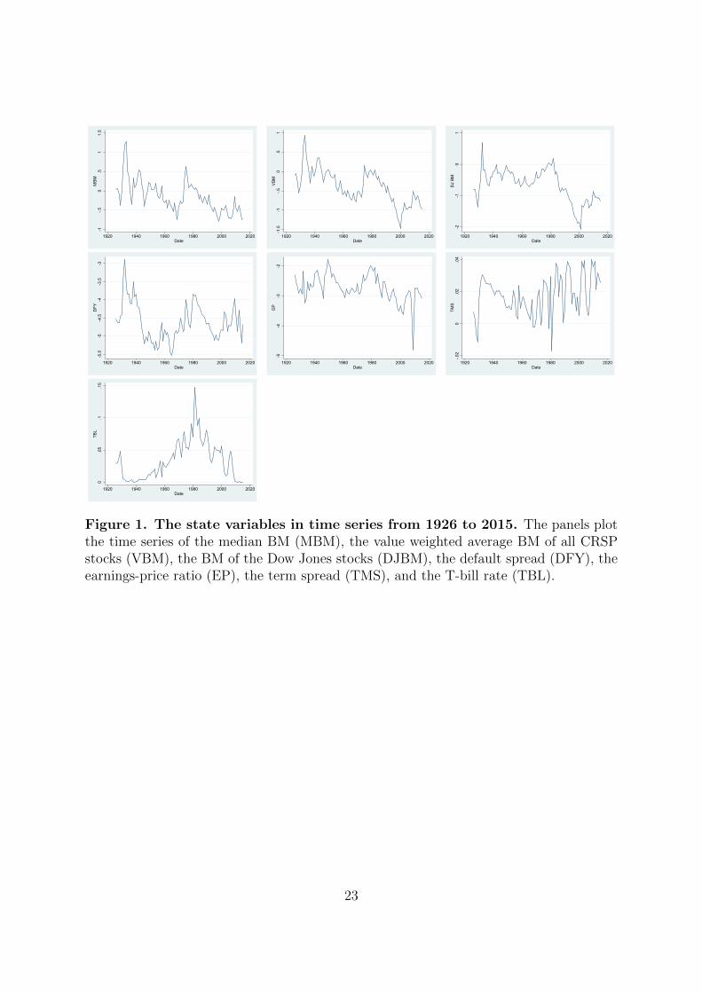
correlations between innovations in the variables are generally weak. Fig. 1, also from

Souza (2017), shows the evolution of the state variables over time between 1926 and 2015.

[Place Table I about here]

[Place Figure 1 about here]

A.2. The backward looking state classification

I classify the market price of risk in each year in high or low based on how the state

variable in that year compares to the variable’s own past values. This ranking is free

from forward looking bias and is the exact same one implemented in Souza (2017) that

also describes it in more details.

Given the historical mean of each state variable in year t, zt, we can calculate the

difference between the value of zt and its historical mean estimated until the previous

year,

Devz,t = zt − zt−1. (23)

Next, we calculate a percentile rank, Γz,t, based on how the deviation at time t, Devz,t,

11Welch and Goyal (2008) describe these variables in more details. The variables are athttp://www.hec.unil.ch/agoyal/.

13

compares with the past deviations until time t,

Γz,t =

∑ti=t0

(I{Devz,i<Devz,t} + 0.5I{Devz,i=Devz,t}

)t− t0 + 1

, (24)

where I{.} is the indicator function. Intuitively, the ranking Γz,t is large when the market

price of risk is unusually far above its historical average.

Table II presents summary statistics for the percentile rankings, still assuming that

they follow a first order AR process. The interpretation is similar to the one for the

original state variables in Table I.

[Place Table II about here]

A.3. The stock returns

I obtain the return data on US stocks, described in details in Fama and French (1993),

from Kenneth French’s data library. The monthly returns from July of 1926 to July of

2015 correspond to the size premium (as the return on the SMB portfolio, Rsmb), the

value premium (as the return on the HML portfolio, Rhml), and the market premium (as

the difference between the return on the market portfolio and the risk free rate, Rmp).

B. Hypotheses tests

B.1. The conditional size premium (H1)

According to the model, the size premium should only be positive if the market price

of risk is above a certain threshold, λt ≥ λ∗. The biggest empirical challenge is that we

do not observe the agents’ private information sets. So the market price of risk is also

unobservable.

14

Let the (observable) threshold for the state variable, Λ∗, be a proxy for λ∗. The time t

expectation of the size premium one period ahead is now

Et[Rsmb,t+1] =

0 Λt < Λ∗

Rsmb,h Λt ≥ Λ∗, (25)

where Λt is the state variable at time t, Λ∗ is the threshold for this state variable, and

Rsmb,h is the mean return on the SMB portfolio considering only the periods in which the

state variable is high (above its threshold):

Rsmb,h =

∑Tt=1 (Rsmb,t IΛt≥Λ∗)∑T

t=1 IΛt≥Λ∗, (26)

where I{} is the indicator function and T is the sample size.

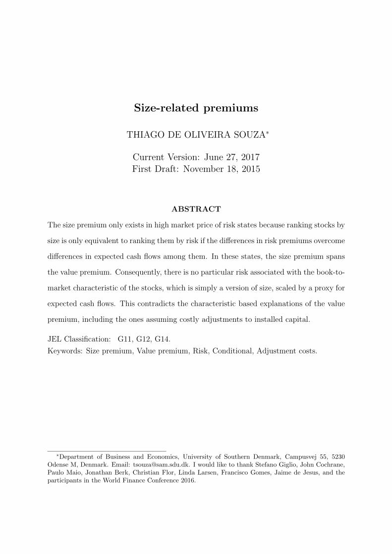
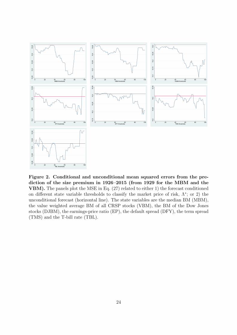
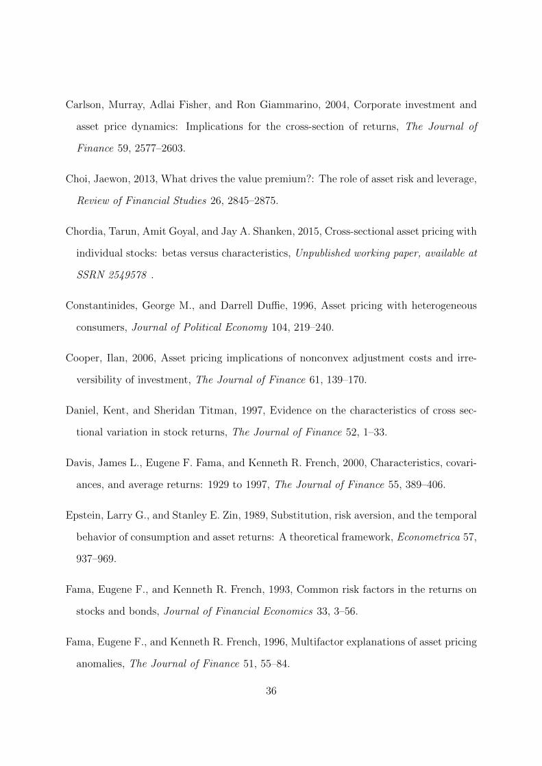
The mean squared error of this forecast (MSE), which is a function of the threshold,

Λ∗, is

MSE(Λ∗) =1

T

T∑t=1

(Et−1[Rsmb,t]−Rsmb,t)2 , (27)

where Et−1[Rsmb,t] is given by Eq. (25). Figure 2 shows the MSE associated with the

possible thresholds, Λ∗, for each state variable.

My first choice for Λ∗ is exactly the one that minimizes the MSE in Eq. (27), denoted

by

Λ∗MSE ≡ arg minΛ∗

MSE(Λ∗). (28)

This choice generates the values in Table III, in which Panel A is in line with the findings

of Souza (2017): The size premium is significant exclusively when the market price of

risk is high, especially for the variables related to aggregate BM ratios. These results also

confirm hypothesis H1 if we assume that the state variables are proxies for the market

price of risk.

15

[Place Table III about here]

B.2. The conditional value premium (H2)

Under the assumption that the BE is a proxy for expected cash flows, the model also

predicts that the value premium should increase with the market price of risk, but it

could still be positive, even if the market price of risk is lower than the threshold below

which the size premium is zero, λt ≤ λ∗.

In this respect, the evidence in Table III, Panel B, shows a significant value premium

when the market price of risk is low, in line with hypothesis H2. The mean value premium

also has larger point estimates when the market price of risk is high according to most

state variables. This might also confirm hypothesis H2. However, the estimates contain

a lot of noise and are statistically insignificant.

It would be interesting to choose Λ∗ so that the value premium is also significant when

the market price of risk is high, Λt ≥ Λ∗. So let us define the equivalent to Eq. (26) for

the value premium,

Rhml,h =

∑Tt=1 (Rhml,t IΛt≥Λ∗)∑T

t=1 IΛt≥Λ∗, (29)

where Rhml,t and Rhml,h are, respectively, the time t return on the HML portfolio and its

mean exclusively when the market price of risk is high.

My second choice for the threshold, denoted by Λ∗HML, is the highest value for the

state variable that generates a mean value premium two standard errors above zero:

Λ∗HML ≡ arg maxΛ∗

= Λ∗

r.t. t(Rsmb,h) ≥ 2

t(Rhml,h) ≥ 2,

(30)

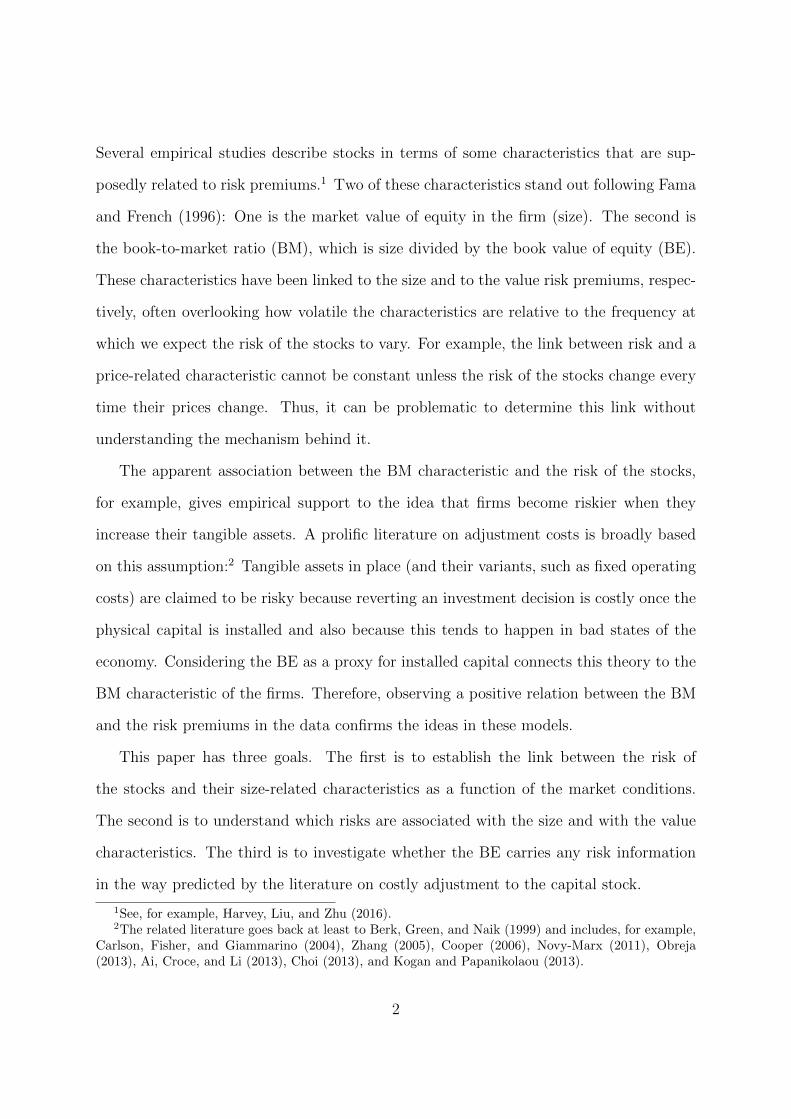
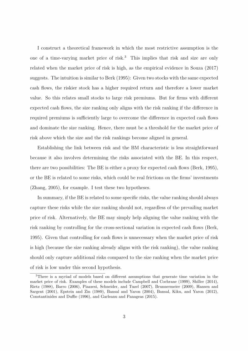
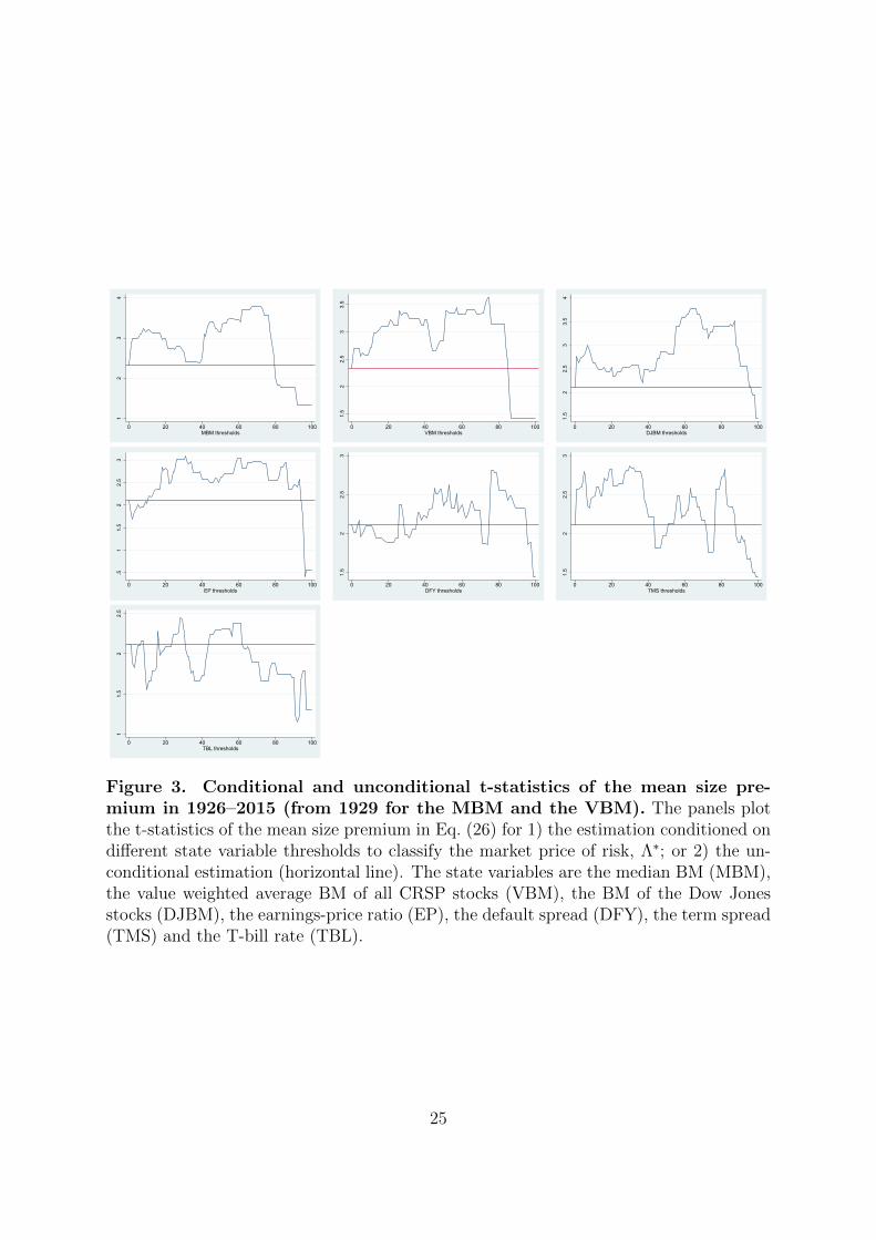
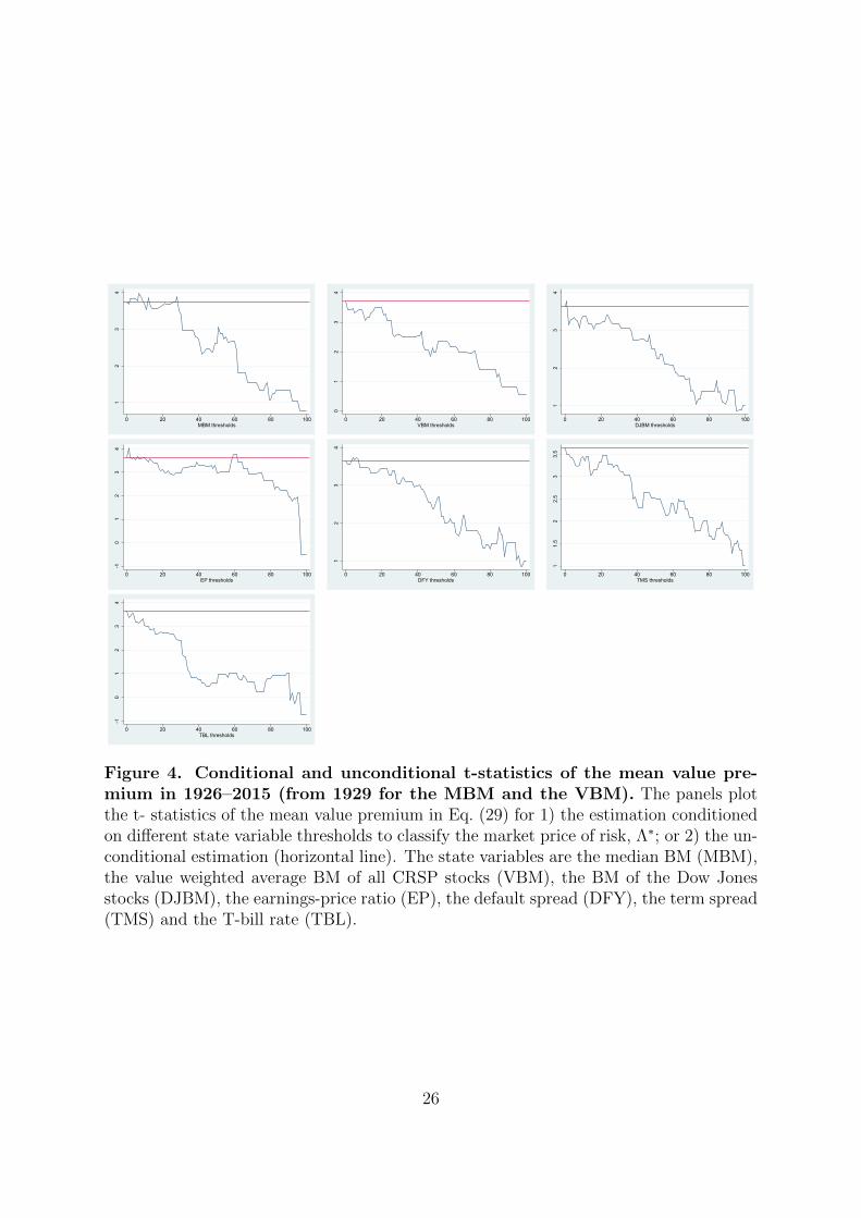
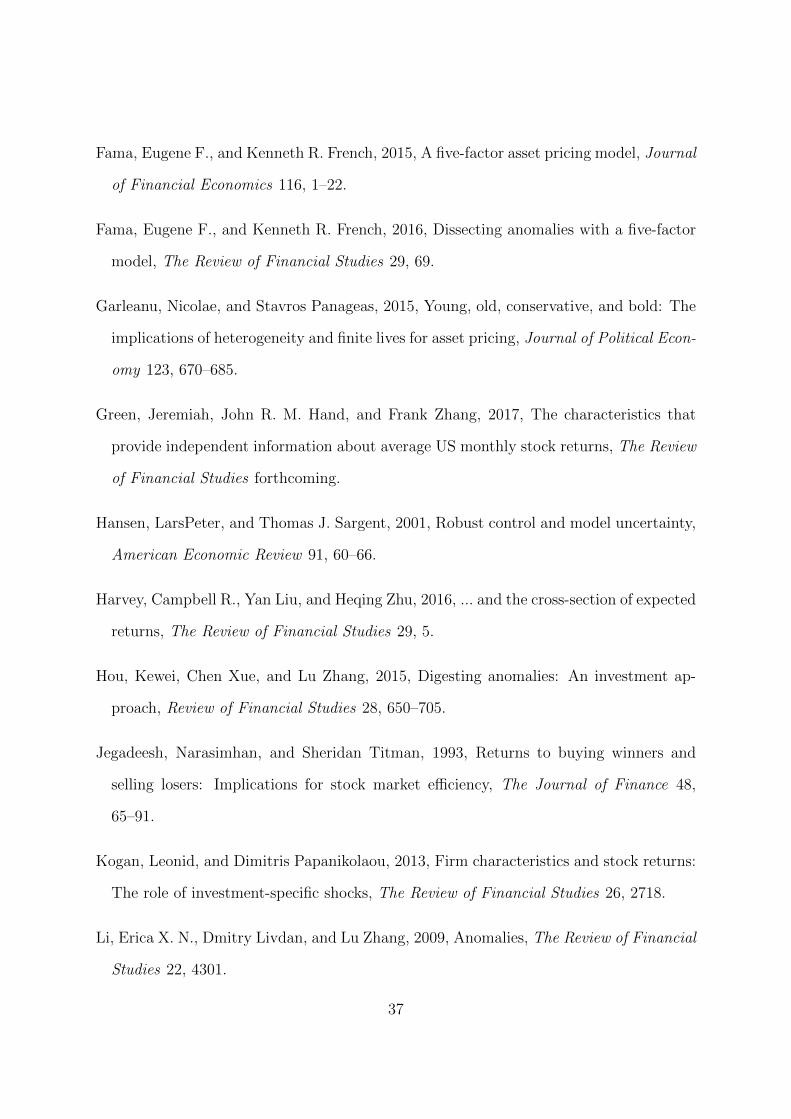
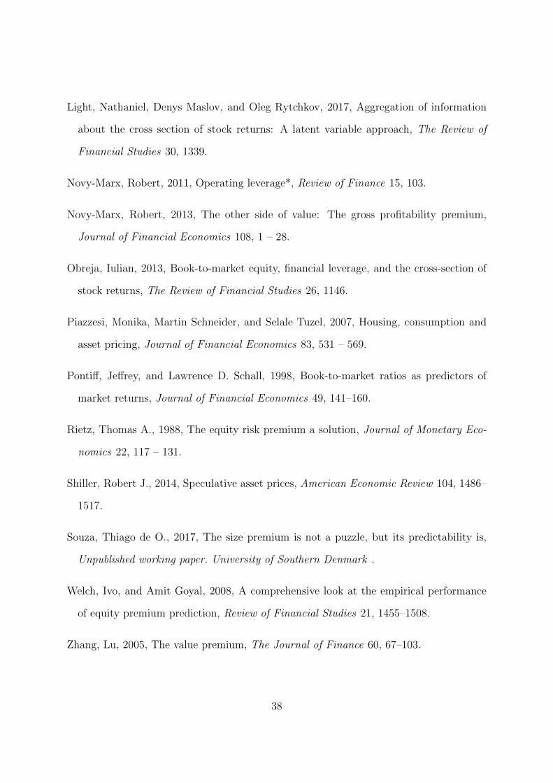
where t(Ri,h) are the t-statistics of the estimated means in Eq. (26) and Eq. (29). Figure 3

16

and Figure 4 show, respectively, how the t-statistics of the mean size and value premiums

change with different thresholds, Λ∗. Effectively, this second threshold, Λ∗HML, is lower

than the first one, Λ∗MSE. Therefore, the sub sample of years in which the market price

of risk is classified as high is larger according to this second classification.

This choice of threshold generates the values in Table VI, in which Panel A is again

consistent with hypothesis H1. Panel B confirms both that the mean value premium is

significant when the market price of risk is low and also that its point estimate tends

to be larger in high market price of risk states. This is consistent with hypothesis H2.

However, we cannot statistically reject the hypothesis that the value premium has the

same mean in both states.

[Place Table VI about here]

B.3. The BE carries no risk information (H3)

Under the assumption that the BE carries no risk information about the stocks, and

is simply a proxy for expected cash flows, the model predicts that the value premium

should be a multiple of the size premium, µhml,t = aµsmb,t, as long as the market price of

risk is high enough, λt > λ∗. We can test this hypothesis empirically by considering the

spanning regression

Rhml,t = αhml + shmlRsmb,t + εhml,t, (31)

where Rhml,t is the return on the HML portfolio at time t, αhml is the constant intercept,

shml is the constant coefficient on the return on the SMB portfolio at time t, Rsmb,t, and

εhml,t is the error term.

17

Under hypothesis H3, the predicted coefficients for this regression are

αhml

> 0 λt < λ∗

= 0 λt ≥ λ∗and shml

= 0 λt < λ∗

> 0 λt ≥ λ∗. (32)

The restriction on the intercept, αhml, in high market price of risk states means that

there is no premium associated with the value portfolios that is not associated with the

size portfolios. And the restriction on the size premium coefficient, shml, means that

the expected premiums associated with the value and the size rankings are significantly

positively correlated (given that they arise in response to the same underlying risks).

But this only happens when the size ranking aligns with the risk ranking as given by

Eq. (11).12 Otherwise, the size ranking captures no priced risks, there should be no cor-

relation between the expected size and value premiums, and the (excess) value premium

should be completely unexplained by the size premium.

The exposure to market risk can also affect the correlation between the returns on

the size and the value portfolios. Including the market premium in Eq. (31) gives

Rhml,t = αhml + βhmlRmp,t + shmlRsmb,t + εhml,t, (33)

where βhml is the constant coefficient on the market premium, Rmp,t. The predicted

coefficients are the same as before, in Eq. (32), but now controlling for the market risk

as well.

This exercise is more informative in the presence of a significant value premium,

that I obtain with the threshold Λ∗HML in Eq. (30). The results, in Table VII, strongly

support the model’s predictions regarding the coefficients in Eq. (32). Panel A shows that

the intercept, αhml, is small and insignificant for every state variable when the market

12In a multivariate setting, this means that the length of the market price of risk vector is large enough,‖λt‖ > ‖λ∗‖.

18

price of risk is high ( except for the TBL without controlling for the market risk). The

correlation between the size and the value premiums are also highly significant for every

state variable, except the TBL after controlling for the market risk. Panel B confirms the

predictions for low market price of risk: Zero correlation between the size and the value

premiums for any state variable, except for the DJBM, and an excess value premium

which is unexplained by the size premium for every state variable.

[Place Table VII about here]

Furthermore, even the different results for the TBL and the DJBM seem to arise

because I use a low threshold for the market price of risk, Λ∗HML, to obtain a significant

value premium. Table IV contains the results for the threshold that minimizes the MSE

of the size premium estimation instead, Λ∗MSE. The only coefficient in this table that

is not exactly in line with the predictions of the model is the insignificant size premium

coefficient, shml, when the market price of risk is high according to the TBL state variable.

And this only happens after controlling for market risk.

Hence, I find no empirical support for the idea that a firm’s BE carries any information

about its risk. In particular, firms with large shares of tangible capital are not riskier

than firms that rely on intangible capital according to the data, at least with the BE as

a proxy for tangible capital. This contradicts the theoretical predictions in the literature

on costly adjustments to the capital stock.

[Place Table IV about here]

B.4. Are there risks associated with size but not with value?

It is also possible that the price ranking captures specific risks that the value ranking

does not capture. Under the hypothesis that the BE is a proxy for expected cash flows,

the value ranking can only possibly improve the price ranking when the market price of

19

risk is low. If Eq. (13) holds, then any ranking different from the size ranking is misaligned

with the risk ranking.

Intuitively, any adjustment remotely related to the expected cash flows helps if the

market price of risk is low because the price ranking is mostly unrelated to risk in this

case. But a less than perfect adjustment to the price ranking should disturb the alignment

with the risk ranking in case this alignment was already good. The proportion of risky

firms in the portfolio of small stocks is already very high if the market price of risk is very

large. Therefore, reshuffling the ranking by some variable that is only an imperfect proxy

for expected cash flows is likely to make the distribution of risk more uniform among the

(value) portfolios.

The equivalent of Eq. (22) for the size premium can be tested with the spanning

regression

Rsmb,t = αsmb + hsmbRhml,t + εsmb,t, (34)

where Rsmb,t is the return on the SMB portfolio at time t, αsmb is the constant intercept,

hsmb is the constant coefficient on the return on the HML portfolio at time t, Rhml,t, and

εsmb,t is the error term. Adding the market premium to the equation, we have

Rsmb,t = αsmb + βsmbRmp,t + hsmbRhml,t + εsmb,t, (35)

where βsmb is the constant coefficient on the market premium.

Under the assumptions that the BE carries no information about risk, the predicted

coefficients for this regression are

αsmb

= 0 λt < λ∗

≥ 0 λt ≥ λ∗and hsmb

= 0 λt < λ∗

> 0 λt ≥ λ∗. (36)

20

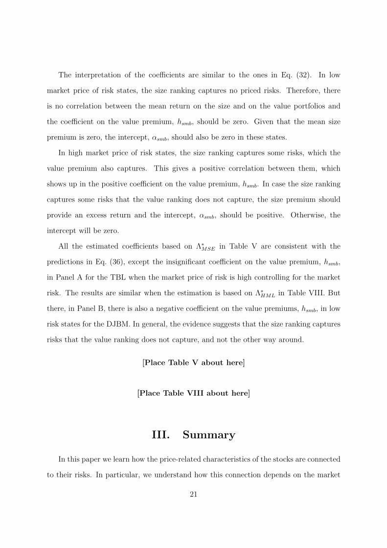
The interpretation of the coefficients are similar to the ones in Eq. (32). In low

market price of risk states, the size ranking captures no priced risks. Therefore, there

is no correlation between the mean return on the size and on the value portfolios and

the coefficient on the value premium, hsmb, should be zero. Given that the mean size

premium is zero, the intercept, αsmb, should also be zero in these states.

In high market price of risk states, the size ranking captures some risks, which the

value premium also captures. This gives a positive correlation between them, which

shows up in the positive coefficient on the value premium, hsmb. In case the size ranking

captures some risks that the value ranking does not capture, the size premium should

provide an excess return and the intercept, αsmb, should be positive. Otherwise, the

intercept will be zero.

All the estimated coefficients based on Λ∗MSE in Table V are consistent with the

predictions in Eq. (36), except the insignificant coefficient on the value premium, hsmb,

in Panel A for the TBL when the market price of risk is high controlling for the market

risk. The results are similar when the estimation is based on Λ∗HML in Table VIII. But

there, in Panel B, there is also a negative coefficient on the value premiums, hsmb, in low

risk states for the DJBM. In general, the evidence suggests that the size ranking captures

risks that the value ranking does not capture, and not the other way around.

[Place Table V about here]

[Place Table VIII about here]

III. Summary

In this paper we learn how the price-related characteristics of the stocks are connected

to their risks. In particular, we understand how this connection depends on the market

21

conditions (the market price of risk) and we learn how we can model this link.

This is important because much of our understanding about Finance is based on the

estimated relation between risk premiums and these characteristics. One example is the

idea that firms that increase their installed capital become riskier given that they face real

investment frictions in bad economic times. This hypothesis seems to receive empirical

support once we consider the BE as a proxy for invested capital and estimate the relation

between the BM characteristic of the firms and their risk premiums.

However, it becomes clear that the BE actually contains no risk information about the

firms once we consider how the market conditions affect the link between risk and the BM

characteristic. Therefore, we also learn that the theory based on costly adjustments to

tangible assets in place is much less consistent with the data than we previously thought.

22

-1-.5

0.5

11.

5M

BM

1920 1940 1960 1980 2000 2020Date

-1.5

-1-.5

0.5

1V

BM

1920 1940 1960 1980 2000 2020Date

-2-1

01

DJ

BM

1920 1940 1960 1980 2000 2020Date

-5.5

-5-4

.5-4

-3.5

-3D

FY

1920 1940 1960 1980 2000 2020Date

-5-4

-3-2

EP

1920 1940 1960 1980 2000 2020Date

-.02

0.0

2.0

4TM

S

1920 1940 1960 1980 2000 2020Date

0.0

5.1

.15

TBL

1920 1940 1960 1980 2000 2020Date

Figure 1. The state variables in time series from 1926 to 2015. The panels plotthe time series of the median BM (MBM), the value weighted average BM of all CRSPstocks (VBM), the BM of the Dow Jones stocks (DJBM), the default spread (DFY), theearnings-price ratio (EP), the term spread (TMS), and the T-bill rate (TBL).

23

10.2

510

.310

.35

10.4

10.4

5

0 20 40 60 80 100MBM thresholds

10.2

510

.310

.35

10.4

10.4

5

0 20 40 60 80 100VBM thresholds

10.1

10.1

510

.210

.25

10.3

0 20 40 60 80 100DJBM thresholds

10.2

10.2

510

.310

.35

0 20 40 60 80 100EP thresholds

10.1

510

.210

.25

10.3

10.3

5

0 20 40 60 80 100DFY thresholds

10.2

10.2

510

.310

.35

0 20 40 60 80 100TMS thresholds

10.2

610

.28

10.3

10.3

210

.34

0 20 40 60 80 100TBL thresholds

Figure 2. Conditional and unconditional mean squared errors from the pre-diction of the size premium in 1926–2015 (from 1929 for the MBM and theVBM). The panels plot the MSE in Eq. (27) related to either 1) the forecast conditionedon different state variable thresholds to classify the market price of risk, Λ∗; or 2) theunconditional forecast (horizontal line). The state variables are the median BM (MBM),the value weighted average BM of all CRSP stocks (VBM), the BM of the Dow Jonesstocks (DJBM), the earnings-price ratio (EP), the default spread (DFY), the term spread(TMS) and the T-bill rate (TBL).

24

12

34


1.5

22.

53

3.5


1.5

22.

53

3.5

4


.51

1.5

22.

53


1.5

22.

53


1.5

22.

53


11.

52

2.5


Figure 3. Conditional and unconditional t-statistics of the mean size pre-mium in 1926–2015 (from 1929 for the MBM and the VBM). The panels plotthe t-statistics of the mean size premium in Eq. (26) for 1) the estimation conditioned ondifferent state variable thresholds to classify the market price of risk, Λ∗; or 2) the un-conditional estimation (horizontal line). The state variables are the median BM (MBM),the value weighted average BM of all CRSP stocks (VBM), the BM of the Dow Jonesstocks (DJBM), the earnings-price ratio (EP), the default spread (DFY), the term spread(TMS) and the T-bill rate (TBL).

25

12

34


01

23

4


12

34


-10

12

34


12

34


11.

52

2.5

33.

5


-10

12

34


Figure 4. Conditional and unconditional t-statistics of the mean value pre-mium in 1926–2015 (from 1929 for the MBM and the VBM). The panels plotthe t- statistics of the mean value premium in Eq. (29) for 1) the estimation conditionedon different state variable thresholds to classify the market price of risk, Λ∗; or 2) the un-conditional estimation (horizontal line). The state variables are the median BM (MBM),the value weighted average BM of all CRSP stocks (VBM), the BM of the Dow Jonesstocks (DJBM), the earnings-price ratio (EP), the default spread (DFY), the term spread(TMS) and the T-bill rate (TBL).

26

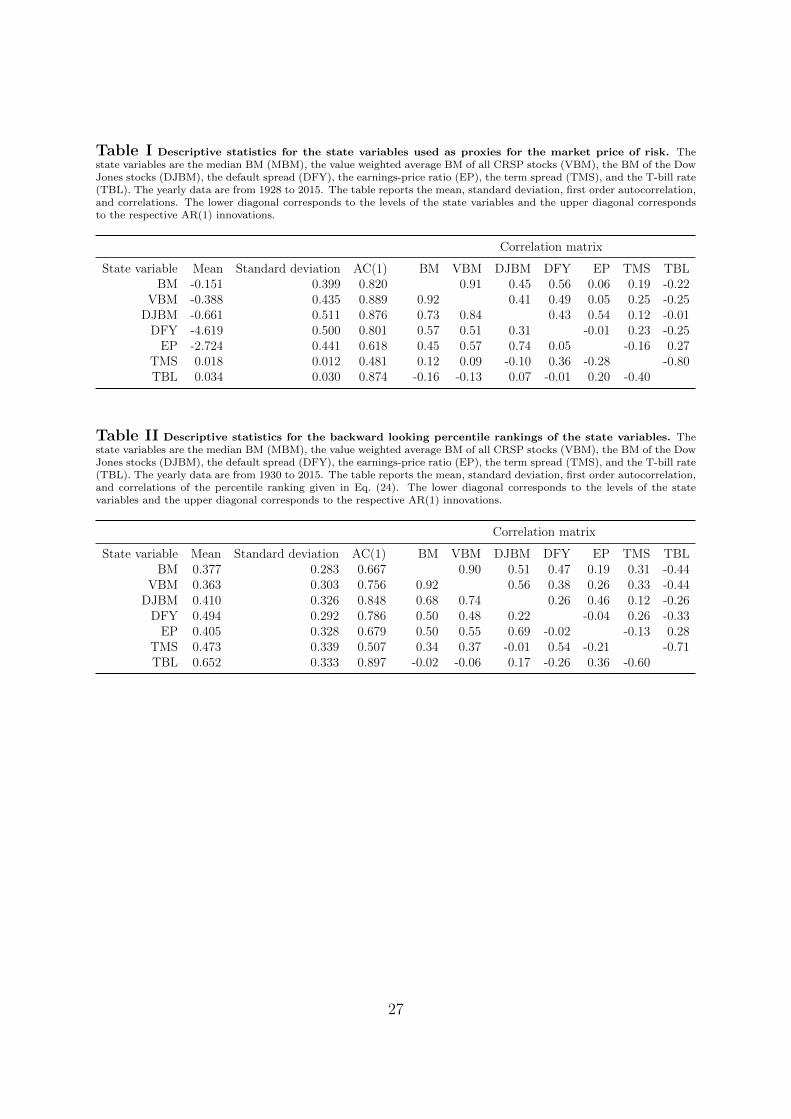
Table I Descriptive statistics for the state variables used as proxies for the market price of risk. Thestate variables are the median BM (MBM), the value weighted average BM of all CRSP stocks (VBM), the BM of the DowJones stocks (DJBM), the default spread (DFY), the earnings-price ratio (EP), the term spread (TMS), and the T-bill rate(TBL). The yearly data are from 1928 to 2015. The table reports the mean, standard deviation, first order autocorrelation,and correlations. The lower diagonal corresponds to the levels of the state variables and the upper diagonal correspondsto the respective AR(1) innovations.

Correlation matrix

State variable Mean Standard deviation AC(1) BM VBM DJBM DFY EP TMS TBLBM -0.151 0.399 0.820 0.91 0.45 0.56 0.06 0.19 -0.22

VBM -0.388 0.435 0.889 0.92 0.41 0.49 0.05 0.25 -0.25DJBM -0.661 0.511 0.876 0.73 0.84 0.43 0.54 0.12 -0.01

DFY -4.619 0.500 0.801 0.57 0.51 0.31 -0.01 0.23 -0.25EP -2.724 0.441 0.618 0.45 0.57 0.74 0.05 -0.16 0.27

TMS 0.018 0.012 0.481 0.12 0.09 -0.10 0.36 -0.28 -0.80TBL 0.034 0.030 0.874 -0.16 -0.13 0.07 -0.01 0.20 -0.40

Table II Descriptive statistics for the backward looking percentile rankings of the state variables. Thestate variables are the median BM (MBM), the value weighted average BM of all CRSP stocks (VBM), the BM of the DowJones stocks (DJBM), the default spread (DFY), the earnings-price ratio (EP), the term spread (TMS), and the T-bill rate(TBL). The yearly data are from 1930 to 2015. The table reports the mean, standard deviation, first order autocorrelation,and correlations of the percentile ranking given in Eq. (24). The lower diagonal corresponds to the levels of the statevariables and the upper diagonal corresponds to the respective AR(1) innovations.

Correlation matrix

State variable Mean Standard deviation AC(1) BM VBM DJBM DFY EP TMS TBLBM 0.377 0.283 0.667 0.90 0.51 0.47 0.19 0.31 -0.44

VBM 0.363 0.303 0.756 0.92 0.56 0.38 0.26 0.33 -0.44DJBM 0.410 0.326 0.848 0.68 0.74 0.26 0.46 0.12 -0.26

DFY 0.494 0.292 0.786 0.50 0.48 0.22 -0.04 0.26 -0.33EP 0.405 0.328 0.679 0.50 0.55 0.69 -0.02 -0.13 0.28

TMS 0.473 0.339 0.507 0.34 0.37 -0.01 0.54 -0.21 -0.71TBL 0.652 0.333 0.897 -0.02 -0.06 0.17 -0.26 0.36 -0.60

27

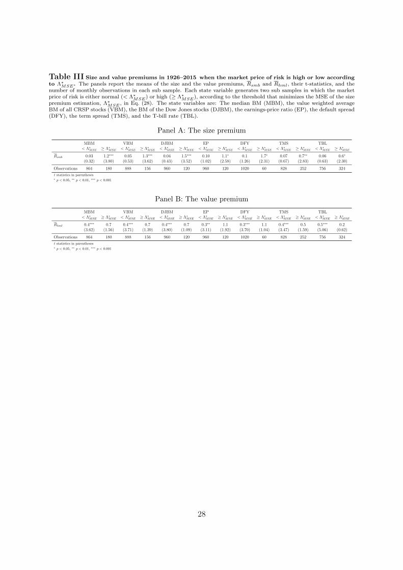
Table III Size and value premiums in 1926–2015 when the market price of risk is high or low accordingto Λ∗

MSE . The panels report the means of the size and the value premiums, Rsmb and Rhml, their t-statistics, and thenumber of monthly observations in each sub sample. Each state variable generates two sub samples in which the marketprice of risk is either normal (< Λ∗

MSE) or high (≥ Λ∗MSE), according to the threshold that minimizes the MSE of the size

premium estimation, Λ∗MSE , in Eq. (28). The state variables are: The median BM (MBM), the value weighted average

BM of all CRSP stocks (VBM), the BM of the Dow Jones stocks (DJBM), the earnings-price ratio (EP), the default spread(DFY), the term spread (TMS), and the T-bill rate (TBL).

Panel A: The size premium

MBM VBM DJBM EP DFY TMS TBL< Λ∗MSE ≥ Λ∗MSE < Λ∗MSE ≥ Λ∗MSE < Λ∗MSE ≥ Λ∗MSE < Λ∗MSE ≥ Λ∗MSE < Λ∗MSE ≥ Λ∗MSE < Λ∗MSE ≥ Λ∗MSE < Λ∗MSE ≥ Λ∗MSE

Rsmb 0.03 1.2∗∗∗ 0.05 1.3∗∗∗ 0.04 1.5∗∗∗ 0.10 1.1∗ 0.1 1.7∗ 0.07 0.7∗∗ 0.06 0.6∗

(0.32) (3.80) (0.53) (3.62) (0.43) (3.52) (1.02) (2.58) (1.26) (2.31) (0.67) (2.83) (0.63) (2.30)

Observations 864 180 888 156 960 120 960 120 1020 60 828 252 756 324

t statistics in parentheses∗ p < 0.05, ∗∗ p < 0.01, ∗∗∗ p < 0.001

Panel B: The value premium

MBM VBM DJBM EP DFY TMS TBL< Λ∗MSE ≥ Λ∗MSE < Λ∗MSE ≥ Λ∗MSE < Λ∗MSE ≥ Λ∗MSE < Λ∗MSE ≥ Λ∗MSE < Λ∗MSE ≥ Λ∗MSE < Λ∗MSE ≥ Λ∗MSE < Λ∗MSE ≥ Λ∗MSE

Rhml 0.4∗∗∗ 0.7 0.4∗∗∗ 0.7 0.4∗∗∗ 0.7 0.3∗∗ 1.1 0.3∗∗∗ 1.1 0.4∗∗∗ 0.5 0.5∗∗∗ 0.2(3.62) (1.56) (3.71) (1.39) (3.80) (1.09) (3.11) (1.92) (3.70) (1.04) (3.47) (1.59) (5.06) (0.62)

Observations 864 180 888 156 960 120 960 120 1020 60 828 252 756 324


28

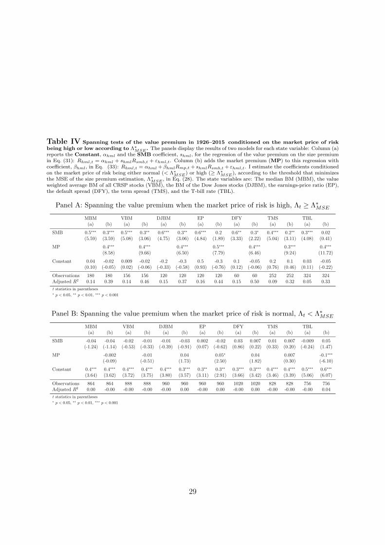
Table IV Spanning tests of the value premium in 1926–2015 conditioned on the market price of riskbeing high or low according to Λ∗

MSE . The panels display the results of two models for each state variable: Column (a)reports the Constant, αhml and the SMB coefficient, shml, for the regression of the value premium on the size premiumin Eq. (31): Rhml,t = αhml + shmlRsmb,t + εhml,t. Column (b) adds the market premium (MP) to this regression withcoefficient, βhml, in Eq. (33): Rhml,t = αhml + βhmlRmp,t + shmlRsmb,t + εhml,t. I estimate the coefficients conditionedon the market price of risk being either normal (< Λ∗

MSE) or high (≥ Λ∗MSE), according to the threshold that minimizes

the MSE of the size premium estimation, Λ∗MSE , in Eq. (28). The state variables are: The median BM (MBM), the value

weighted average BM of all CRSP stocks (VBM), the BM of the Dow Jones stocks (DJBM), the earnings-price ratio (EP),the default spread (DFY), the term spread (TMS), and the T-bill rate (TBL).

Panel A: Spanning the value premium when the market price of risk is high, Λt ≥ Λ∗MSE

MBM VBM DJBM EP DFY TMS TBL(a) (b) (a) (b) (a) (b) (a) (b) (a) (b) (a) (b) (a) (b)

SMB 0.5∗∗∗ 0.3∗∗∗ 0.5∗∗∗ 0.3∗∗ 0.6∗∗∗ 0.3∗∗ 0.6∗∗∗ 0.2 0.6∗∗ 0.3∗ 0.4∗∗∗ 0.2∗∗ 0.3∗∗∗ 0.02(5.59) (3.59) (5.08) (3.06) (4.75) (3.06) (4.84) (1.89) (3.33) (2.22) (5.04) (3.11) (4.08) (0.41)

MP 0.4∗∗∗ 0.4∗∗∗ 0.4∗∗∗ 0.5∗∗∗ 0.4∗∗∗ 0.3∗∗∗ 0.4∗∗∗

(8.58) (9.66) (6.50) (7.79) (6.46) (9.24) (11.72)

Constant 0.04 -0.02 0.009 -0.02 -0.2 -0.3 0.5 -0.3 0.1 -0.05 0.2 0.1 0.03 -0.05(0.10) (-0.05) (0.02) (-0.06) (-0.33) (-0.58) (0.93) (-0.76) (0.12) (-0.06) (0.76) (0.46) (0.11) (-0.22)

Observations 180 180 156 156 120 120 120 120 60 60 252 252 324 324Adjusted R2 0.14 0.39 0.14 0.46 0.15 0.37 0.16 0.44 0.15 0.50 0.09 0.32 0.05 0.33


Panel B: Spanning the value premium when the market price of risk is normal, Λt < Λ∗MSE


SMB -0.04 -0.04 -0.02 -0.01 -0.01 -0.03 0.002 -0.02 0.03 0.007 0.01 0.007 -0.009 0.05(-1.24) (-1.14) (-0.53) (-0.33) (-0.39) (-0.91) (0.07) (-0.62) (0.86) (0.22) (0.33) (0.20) (-0.24) (1.47)

MP -0.002 -0.01 0.04 0.05∗ 0.04 0.007 -0.1∗∗∗

(-0.09) (-0.51) (1.73) (2.50) (1.82) (0.30) (-6.10)

Constant 0.4∗∗∗ 0.4∗∗∗ 0.4∗∗∗ 0.4∗∗∗ 0.4∗∗∗ 0.3∗∗∗ 0.3∗∗ 0.3∗∗ 0.3∗∗∗ 0.3∗∗∗ 0.4∗∗∗ 0.4∗∗∗ 0.5∗∗∗ 0.6∗∗∗

(3.64) (3.62) (3.72) (3.75) (3.80) (3.57) (3.11) (2.91) (3.66) (3.42) (3.46) (3.39) (5.06) (6.07)

Observations 864 864 888 888 960 960 960 960 1020 1020 828 828 756 756Adjusted R2 0.00 -0.00 -0.00 -0.00 -0.00 0.00 -0.00 0.00 -0.00 0.00 -0.00 -0.00 -0.00 0.04


29

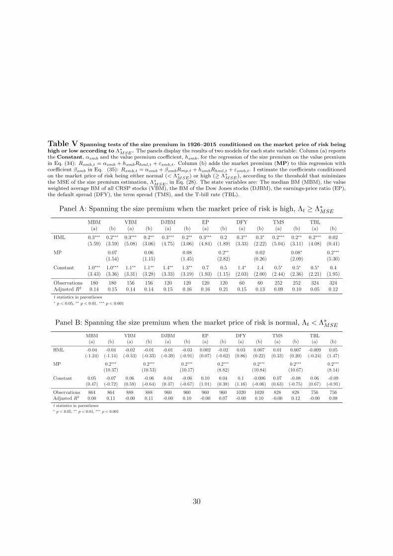
Table V Spanning tests of the size premium in 1926–2015 conditioned on the market price of risk beinghigh or low according to Λ∗

MSE . The panels display the results of two models for each state variable: Column (a) reportsthe Constant, αsmb and the value premium coefficient, hsmb, for the regression of the size premium on the value premiumin Eq. (34): Rsmb,t = αsmb + hsmbRhml,t + εsmb,t. Column (b) adds the market premium (MP) to this regression withcoefficient βsmb in Eq. (35): Rsmb,t = αsmb + βsmbRmp,t + hsmbRhml,t + εsmb,t. I estimate the coefficients conditionedon the market price of risk being either normal (< Λ∗

MSE) or high (≥ Λ∗MSE), according to the threshold that minimizes

the MSE of the size premium estimation, Λ∗MSE , in Eq. (28). The state variables are: The median BM (MBM), the value

weighted average BM of all CRSP stocks (VBM), the BM of the Dow Jones stocks (DJBM), the earnings-price ratio (EP),the default spread (DFY), the term spread (TMS), and the T-bill rate (TBL).

Panel A: Spanning the size premium when the market price of risk is high, Λt ≥ Λ∗MSE


HML 0.3∗∗∗ 0.2∗∗∗ 0.3∗∗∗ 0.2∗∗ 0.3∗∗∗ 0.2∗∗ 0.3∗∗∗ 0.2 0.3∗∗ 0.3∗ 0.2∗∗∗ 0.2∗∗ 0.2∗∗∗ 0.02(5.59) (3.59) (5.08) (3.06) (4.75) (3.06) (4.84) (1.89) (3.33) (2.22) (5.04) (3.11) (4.08) (0.41)

MP 0.07 0.06 0.08 0.2∗∗ 0.02 0.08∗ 0.2∗∗∗

(1.54) (1.15) (1.45) (2.82) (0.26) (2.09) (5.30)

Constant 1.0∗∗∗ 1.0∗∗∗ 1.1∗∗ 1.1∗∗ 1.4∗∗ 1.3∗∗ 0.7 0.5 1.4∗ 1.4 0.5∗ 0.5∗ 0.5∗ 0.4(3.43) (3.36) (3.31) (3.28) (3.33) (3.19) (1.93) (1.15) (2.03) (2.00) (2.44) (2.36) (2.21) (1.95)



Panel B: Spanning the size premium when the market price of risk is normal, Λt < Λ∗MSE


HML -0.04 -0.04 -0.02 -0.01 -0.01 -0.03 0.002 -0.02 0.03 0.007 0.01 0.007 -0.009 0.05(-1.24) (-1.14) (-0.53) (-0.33) (-0.39) (-0.91) (0.07) (-0.62) (0.86) (0.22) (0.33) (0.20) (-0.24) (1.47)

MP 0.2∗∗∗ 0.2∗∗∗ 0.2∗∗∗ 0.2∗∗∗ 0.2∗∗∗ 0.2∗∗∗ 0.2∗∗∗

(10.37) (10.53) (10.17) (8.82) (10.84) (10.67) (8.14)

Constant 0.05 -0.07 0.06 -0.06 0.04 -0.06 0.10 0.04 0.1 -0.006 0.07 -0.08 0.06 -0.09(0.47) (-0.72) (0.59) (-0.64) (0.47) (-0.67) (1.01) (0.38) (1.16) (-0.06) (0.63) (-0.75) (0.67) (-0.91)

Observations 864 864 888 888 960 960 960 960 1020 1020 828 828 756 756Adjusted R2 0.00 0.11 -0.00 0.11 -0.00 0.10 -0.00 0.07 -0.00 0.10 -0.00 0.12 -0.00 0.08


30

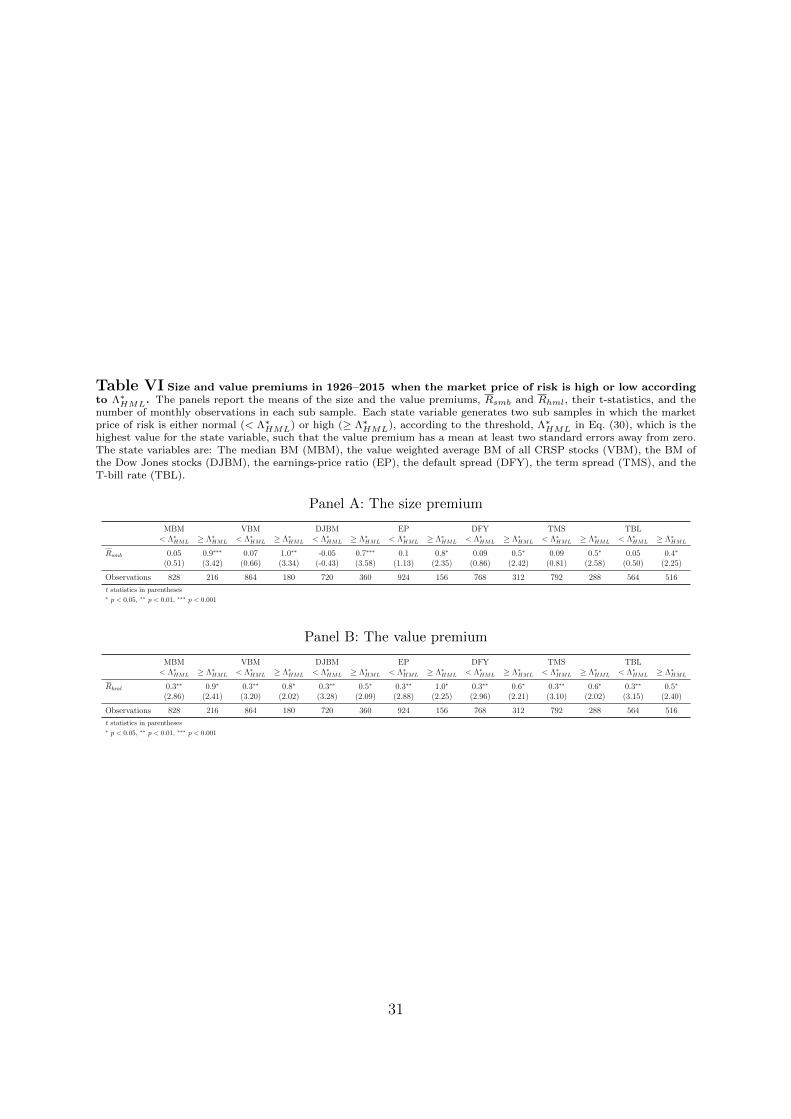
Table VI Size and value premiums in 1926–2015 when the market price of risk is high or low accordingto Λ∗

HML. The panels report the means of the size and the value premiums, Rsmb and Rhml, their t-statistics, and thenumber of monthly observations in each sub sample. Each state variable generates two sub samples in which the marketprice of risk is either normal (< Λ∗

HML) or high (≥ Λ∗HML), according to the threshold, Λ∗

HML in Eq. (30), which is thehighest value for the state variable, such that the value premium has a mean at least two standard errors away from zero.The state variables are: The median BM (MBM), the value weighted average BM of all CRSP stocks (VBM), the BM ofthe Dow Jones stocks (DJBM), the earnings-price ratio (EP), the default spread (DFY), the term spread (TMS), and theT-bill rate (TBL).

Panel A: The size premium

MBM VBM DJBM EP DFY TMS TBL< Λ∗HML ≥ Λ∗HML < Λ∗HML ≥ Λ∗HML < Λ∗HML ≥ Λ∗HML < Λ∗HML ≥ Λ∗HML < Λ∗HML ≥ Λ∗HML < Λ∗HML ≥ Λ∗HML < Λ∗HML ≥ Λ∗HML

Rsmb 0.05 0.9∗∗∗ 0.07 1.0∗∗ -0.05 0.7∗∗∗ 0.1 0.8∗ 0.09 0.5∗ 0.09 0.5∗ 0.05 0.4∗

(0.51) (3.42) (0.66) (3.34) (-0.43) (3.58) (1.13) (2.35) (0.86) (2.42) (0.81) (2.58) (0.50) (2.25)

Observations 828 216 864 180 720 360 924 156 768 312 792 288 564 516


Panel B: The value premium

MBM VBM DJBM EP DFY TMS TBL< Λ∗HML ≥ Λ∗HML < Λ∗HML ≥ Λ∗HML < Λ∗HML ≥ Λ∗HML < Λ∗HML ≥ Λ∗HML < Λ∗HML ≥ Λ∗HML < Λ∗HML ≥ Λ∗HML < Λ∗HML ≥ Λ∗HML

Rhml 0.3∗∗ 0.9∗ 0.3∗∗ 0.8∗ 0.3∗∗ 0.5∗ 0.3∗∗ 1.0∗ 0.3∗∗ 0.6∗ 0.3∗∗ 0.6∗ 0.3∗∗ 0.5∗

(2.86) (2.41) (3.20) (2.02) (3.28) (2.09) (2.88) (2.25) (2.96) (2.21) (3.10) (2.02) (3.15) (2.40)

Observations 828 216 864 180 720 360 924 156 768 312 792 288 564 516


31

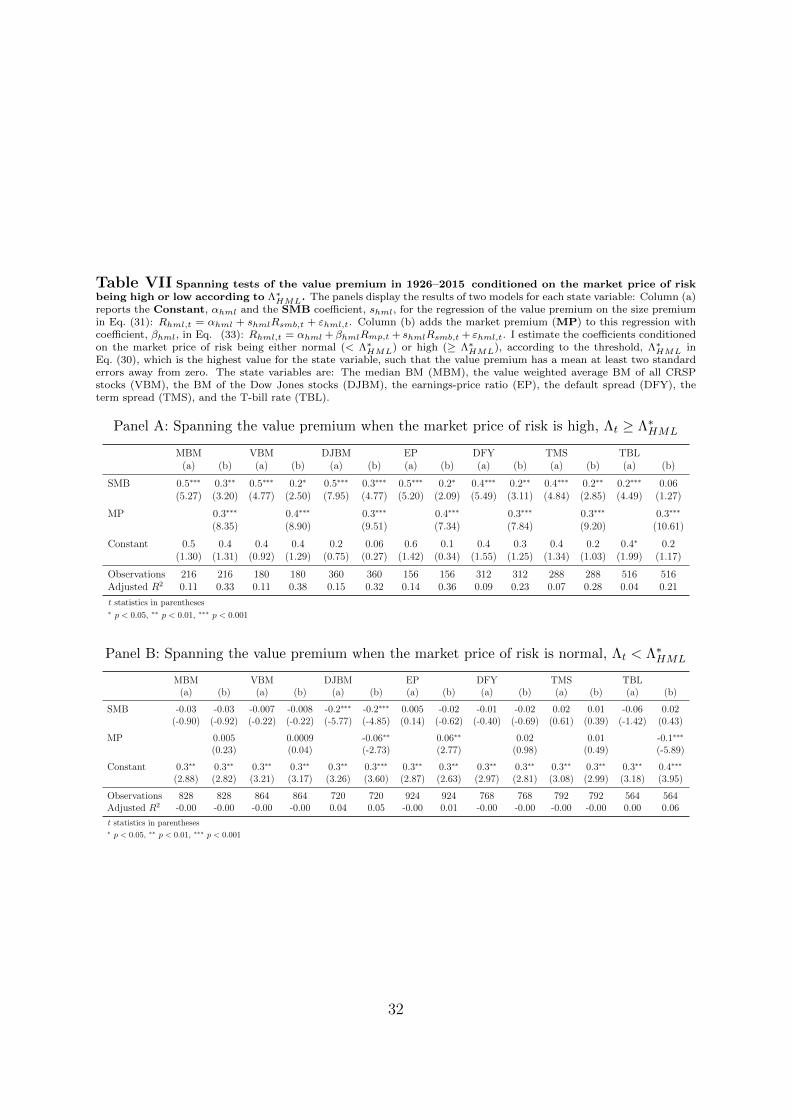
Table VII Spanning tests of the value premium in 1926–2015 conditioned on the market price of riskbeing high or low according to Λ∗

HML. The panels display the results of two models for each state variable: Column (a)reports the Constant, αhml and the SMB coefficient, shml, for the regression of the value premium on the size premiumin Eq. (31): Rhml,t = αhml + shmlRsmb,t + εhml,t. Column (b) adds the market premium (MP) to this regression withcoefficient, βhml, in Eq. (33): Rhml,t = αhml + βhmlRmp,t + shmlRsmb,t + εhml,t. I estimate the coefficients conditionedon the market price of risk being either normal (< Λ∗

HML) or high (≥ Λ∗HML), according to the threshold, Λ∗

HML inEq. (30), which is the highest value for the state variable, such that the value premium has a mean at least two standarderrors away from zero. The state variables are: The median BM (MBM), the value weighted average BM of all CRSPstocks (VBM), the BM of the Dow Jones stocks (DJBM), the earnings-price ratio (EP), the default spread (DFY), theterm spread (TMS), and the T-bill rate (TBL).

Panel A: Spanning the value premium when the market price of risk is high, Λt ≥ Λ∗HML


SMB 0.5∗∗∗ 0.3∗∗ 0.5∗∗∗ 0.2∗ 0.5∗∗∗ 0.3∗∗∗ 0.5∗∗∗ 0.2∗ 0.4∗∗∗ 0.2∗∗ 0.4∗∗∗ 0.2∗∗ 0.2∗∗∗ 0.06(5.27) (3.20) (4.77) (2.50) (7.95) (4.77) (5.20) (2.09) (5.49) (3.11) (4.84) (2.85) (4.49) (1.27)

MP 0.3∗∗∗ 0.4∗∗∗ 0.3∗∗∗ 0.4∗∗∗ 0.3∗∗∗ 0.3∗∗∗ 0.3∗∗∗

(8.35) (8.90) (9.51) (7.34) (7.84) (9.20) (10.61)

Constant 0.5 0.4 0.4 0.4 0.2 0.06 0.6 0.1 0.4 0.3 0.4 0.2 0.4∗ 0.2(1.30) (1.31) (0.92) (1.29) (0.75) (0.27) (1.42) (0.34) (1.55) (1.25) (1.34) (1.03) (1.99) (1.17)



Panel B: Spanning the value premium when the market price of risk is normal, Λt < Λ∗HML


SMB -0.03 -0.03 -0.007 -0.008 -0.2∗∗∗ -0.2∗∗∗ 0.005 -0.02 -0.01 -0.02 0.02 0.01 -0.06 0.02(-0.90) (-0.92) (-0.22) (-0.22) (-5.77) (-4.85) (0.14) (-0.62) (-0.40) (-0.69) (0.61) (0.39) (-1.42) (0.43)

MP 0.005 0.0009 -0.06∗∗ 0.06∗∗ 0.02 0.01 -0.1∗∗∗

(0.23) (0.04) (-2.73) (2.77) (0.98) (0.49) (-5.89)

Constant 0.3∗∗ 0.3∗∗ 0.3∗∗ 0.3∗∗ 0.3∗∗ 0.3∗∗∗ 0.3∗∗ 0.3∗∗ 0.3∗∗ 0.3∗∗ 0.3∗∗ 0.3∗∗ 0.3∗∗ 0.4∗∗∗

(2.88) (2.82) (3.21) (3.17) (3.26) (3.60) (2.87) (2.63) (2.97) (2.81) (3.08) (2.99) (3.18) (3.95)

Observations 828 828 864 864 720 720 924 924 768 768 792 792 564 564Adjusted R2 -0.00 -0.00 -0.00 -0.00 0.04 0.05 -0.00 0.01 -0.00 -0.00 -0.00 -0.00 0.00 0.06


32

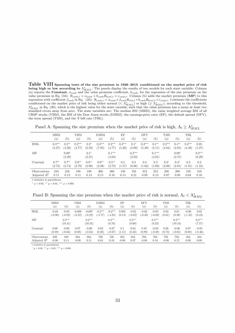
Table VIII Spanning tests of the size premium in 1926–2015 conditioned on the market price of riskbeing high or low according to Λ∗

HML. The panels display the results of two models for each state variable: Column(a) reports the Constant, αsmb and the value premium coefficient, hsmb, for the regression of the size premium on thevalue premium in Eq. (34): Rsmb,t = αsmb + hsmbRhml,t + εsmb,t. Column (b) adds the market premium (MP) to thisregression with coefficient βsmb in Eq. (35): Rsmb,t = αsmb+βsmbRmp,t+hsmbRhml,t+εsmb,t. I estimate the coefficientsconditioned on the market price of risk being either normal (< Λ∗

HML) or high (≥ Λ∗HML), according to the threshold,

Λ∗HML in Eq. (30), which is the highest value for the state variable, such that the value premium has a mean at least two

standard errors away from zero. The state variables are: The median BM (MBM), the value weighted average BM of allCRSP stocks (VBM), the BM of the Dow Jones stocks (DJBM), the earnings-price ratio (EP), the default spread (DFY),the term spread (TMS), and the T-bill rate (TBL).

Panel A: Spanning the size premium when the market price of risk is high, Λt ≥ Λ∗HML


HML 0.3∗∗∗ 0.2∗∗ 0.2∗∗∗ 0.2∗ 0.3∗∗∗ 0.2∗∗∗ 0.3∗∗∗ 0.1∗ 0.2∗∗∗ 0.1∗∗ 0.2∗∗∗ 0.1∗∗ 0.2∗∗∗ 0.05(5.27) (3.20) (4.77) (2.50) (7.95) (4.77) (5.20) (2.09) (5.49) (3.11) (4.84) (2.85) (4.49) (1.27)

MP 0.09∗ 0.1∗ 0.1∗∗∗ 0.2∗∗∗ 0.1∗∗∗ 0.09∗ 0.2∗∗∗

(2.28) (2.21) (4.03) (3.83) (4.01) (2.57) (6.29)

Constant 0.7∗∗ 0.7∗∗ 0.8∗∗ 0.8∗∗ 0.6∗∗ 0.5∗∗ 0.5 0.3 0.4 0.3 0.4∗ 0.4∗ 0.3 0.2(2.72) (2.74) (2.79) (2.90) (2.98) (2.72) (1.57) (0.98) (1.82) (1.69) (2.08) (2.01) (1.81) (1.34)



Panel B: Spanning the size premium when the market price of risk is normal, Λt < Λ∗HML


HML -0.03 -0.03 -0.008 -0.007 -0.2∗∗∗ -0.2∗∗∗ 0.005 -0.02 -0.02 -0.03 0.02 0.01 -0.06 0.02(-0.90) (-0.92) (-0.22) (-0.22) (-5.77) (-4.85) (0.14) (-0.62) (-0.40) (-0.69) (0.61) (0.39) (-1.42) (0.43)

MP 0.2∗∗∗ 0.2∗∗∗ 0.2∗∗∗ 0.2∗∗∗ 0.2∗∗∗ 0.2∗∗∗ 0.2∗∗∗

(10.41) (10.35) (6.76) (8.60) (9.23) (10.54) (7.57)

Constant 0.06 -0.06 0.07 -0.06 0.03 -0.07 0.1 0.04 0.10 -0.03 0.08 -0.06 0.07 -0.05(0.59) (-0.64) (0.68) (-0.64) (0.26) (-0.67) (1.11) (0.42) (0.89) (-0.28) (0.73) (-0.61) (0.68) (-0.46)

Observations 828 828 864 864 720 720 924 924 768 768 792 792 564 564Adjusted R2 -0.00 0.11 -0.00 0.11 0.04 0.10 -0.00 0.07 -0.00 0.10 -0.00 0.12 0.00 0.09


33

Appendix A. Multivariate derivation

In a multidimensional setting, the SDF in Eq. (1) becomes

dζt = −ζt[rft dt+ λ>t dz1t], (A1)

where dz1t is a multi-dimensional standard Brownian motion and λt, is the multi-

dimensional stochastic process representing the market price of risk at time t associated

to each risk source. We also adjust the price process in Eq. (2) to

dPit = Pit[µit dt+ σ>it , dz1t + σ̃>it dzt], (A2)

where σit is now a multi-dimensional stochastic process, and dzt is independent of dz1t.

The multi-dimensional equivalent to the expected excess rate of return in Eq. (3) is now

µit − rft = σ>itλt, (A3)

and the multi-dimensional equivalent of Eq. (5) gives the return on the SMB and HML

portfolios, respectively, as

µsmb,t = σ>smb,tλt, (A4)

µhml,t = σ>hml,tλt. (A5)

The main difference with the one-dimensional formulation is that with a single risk source

the premiums on small and value stocks (and indeed all risk premiums) must be perfectly

correlated given that there is only one priced risk in the economy.

34

REFERENCES

Ai, Hengjie, Mariano Massimiliano Croce, and Kai Li, 2013, Toward a quantitative gen-

eral equilibrium asset pricing model with intangible capital, The Review of Financial

Studies 26, 491.

Bansal, Ravi, Dana Kiku, and Amir Yaron, 2012, An empirical evaluation of the long-run

risks model for asset prices, Critical Finance Review 1, 183–221.

Bansal, Ravi, and Amir Yaron, 2004, Risks for the long run: A potential resolution of

asset pricing puzzles, The Journal of Finance 59, 1481–1509.

Banz, Rolf W., 1981, The relationship between return and market value of common

stocks, Journal of Financial Economics 9, 3–18.

Barro, Robert J., 2006, Rare disasters and asset markets in the twentieth century*, The

Quarterly Journal of Economics 121, 823.

Berk, Jonathan B., 1995, A critique of size-related anomalies, Review of Financial Studies

8, 275–286.

Berk, Jonathan B., Richard C. Green, and Vasant Naik, 1999, Optimal investment,

growth options, and security returns, The Journal of Finance 54, 1553–1607.

Brunnermeier, Markus K., 2009, Deciphering the liquidity and credit crunch 2007-2008,

Journal of Economic Perspectives 23, 77–100.

Campbell, John Y., and John H. Cochrane, 1999, By force of habit: A consumptionbased

explanation of aggregate stock market behavior, Journal of Political Economy 107,

205–251.

35

Carlson, Murray, Adlai Fisher, and Ron Giammarino, 2004, Corporate investment and

asset price dynamics: Implications for the cross-section of returns, The Journal of

Finance 59, 2577–2603.

Choi, Jaewon, 2013, What drives the value premium?: The role of asset risk and leverage,

Review of Financial Studies 26, 2845–2875.

Chordia, Tarun, Amit Goyal, and Jay A. Shanken, 2015, Cross-sectional asset pricing with

individual stocks: betas versus characteristics, Unpublished working paper, available at

SSRN 2549578 .

Constantinides, George M., and Darrell Duffie, 1996, Asset pricing with heterogeneous

consumers, Journal of Political Economy 104, 219–240.

Cooper, Ilan, 2006, Asset pricing implications of nonconvex adjustment costs and irre-

versibility of investment, The Journal of Finance 61, 139–170.

Daniel, Kent, and Sheridan Titman, 1997, Evidence on the characteristics of cross sec-

tional variation in stock returns, The Journal of Finance 52, 1–33.

Davis, James L., Eugene F. Fama, and Kenneth R. French, 2000, Characteristics, covari-

ances, and average returns: 1929 to 1997, The Journal of Finance 55, 389–406.

Epstein, Larry G., and Stanley E. Zin, 1989, Substitution, risk aversion, and the temporal

behavior of consumption and asset returns: A theoretical framework, Econometrica 57,

937–969.

Fama, Eugene F., and Kenneth R. French, 1993, Common risk factors in the returns on

stocks and bonds, Journal of Financial Economics 33, 3–56.

Fama, Eugene F., and Kenneth R. French, 1996, Multifactor explanations of asset pricing

anomalies, The Journal of Finance 51, 55–84.

36

Fama, Eugene F., and Kenneth R. French, 2015, A five-factor asset pricing model, Journal

of Financial Economics 116, 1–22.

Fama, Eugene F., and Kenneth R. French, 2016, Dissecting anomalies with a five-factor

model, The Review of Financial Studies 29, 69.

Garleanu, Nicolae, and Stavros Panageas, 2015, Young, old, conservative, and bold: The

implications of heterogeneity and finite lives for asset pricing, Journal of Political Econ-

omy 123, 670–685.

Green, Jeremiah, John R. M. Hand, and Frank Zhang, 2017, The characteristics that

provide independent information about average US monthly stock returns, The Review

of Financial Studies forthcoming.

Hansen, LarsPeter, and Thomas J. Sargent, 2001, Robust control and model uncertainty,

American Economic Review 91, 60–66.

Harvey, Campbell R., Yan Liu, and Heqing Zhu, 2016, ... and the cross-section of expected

returns, The Review of Financial Studies 29, 5.

Hou, Kewei, Chen Xue, and Lu Zhang, 2015, Digesting anomalies: An investment ap-

proach, Review of Financial Studies 28, 650–705.

Jegadeesh, Narasimhan, and Sheridan Titman, 1993, Returns to buying winners and

selling losers: Implications for stock market efficiency, The Journal of Finance 48,

65–91.

Kogan, Leonid, and Dimitris Papanikolaou, 2013, Firm characteristics and stock returns:

The role of investment-specific shocks, The Review of Financial Studies 26, 2718.

Li, Erica X. N., Dmitry Livdan, and Lu Zhang, 2009, Anomalies, The Review of Financial

Studies 22, 4301.

37

Light, Nathaniel, Denys Maslov, and Oleg Rytchkov, 2017, Aggregation of information

about the cross section of stock returns: A latent variable approach, The Review of

Financial Studies 30, 1339.

Novy-Marx, Robert, 2011, Operating leverage*, Review of Finance 15, 103.

Novy-Marx, Robert, 2013, The other side of value: The gross profitability premium,

Journal of Financial Economics 108, 1 – 28.

Obreja, Iulian, 2013, Book-to-market equity, financial leverage, and the cross-section of

stock returns, The Review of Financial Studies 26, 1146.

Piazzesi, Monika, Martin Schneider, and Selale Tuzel, 2007, Housing, consumption and

asset pricing, Journal of Financial Economics 83, 531 – 569.

Pontiff, Jeffrey, and Lawrence D. Schall, 1998, Book-to-market ratios as predictors of

market returns, Journal of Financial Economics 49, 141–160.

Rietz, Thomas A., 1988, The equity risk premium a solution, Journal of Monetary Eco-

nomics 22, 117 – 131.

Shiller, Robert J., 2014, Speculative asset prices, American Economic Review 104, 1486–

1517.

Souza, Thiago de O., 2017, The size premium is not a puzzle, but its predictability is,

Unpublished working paper. University of Southern Denmark .

Welch, Ivo, and Amit Goyal, 2008, A comprehensive look at the empirical performance

of equity premium prediction, Review of Financial Studies 21, 1455–1508.

Zhang, Lu, 2005, The value premium, The Journal of Finance 60, 67–103.

38

Documents

Size-related premiums