SMOTEâ€“IPF: Addressing the noisy and borderline examples

Information Sciences 291 (2015) 184–203

Contents lists available at ScienceDirect

Information Sciences

journal homepage: www.elsevier .com/locate / ins

SMOTE–IPF: Addressing the noisy and borderline examplesproblem in imbalanced classification by a re-sampling methodwith filtering

http://dx.doi.org/10.1016/j.ins.2014.08.0510020-0255/� 2014 Elsevier Inc. All rights reserved.

⇑ Corresponding author. Tel.: +34 958 240598; fax: +34 958 243317.E-mail addresses: [email protected] (J.A. Sáez), [email protected] (J. Luengo), [email protected] (J. Stefanowski), herrera@decs

(F. Herrera).

José A. Sáez a,⇑, Julián Luengo b, Jerzy Stefanowski c, Francisco Herrera a

a Department of Computer Science and Artificial Intelligence, University of Granada, CITIC-UGR, Granada 18071, Spainb Department of Civil Engineering, LSI, University of Burgos, Burgos 09006, Spainc Institute of Computing Science, Poznan University of Technology, ul. Piotrowo 2, 60-965 Poznan, Poland

a r t i c l e i n f o

Article history:Received 9 April 2013Received in revised form 20 May 2014Accepted 26 August 2014Available online 4 September 2014

Keywords:Imbalanced classificationBorderline examplesNoisy dataNoise filtersSMOTE

a b s t r a c t

Classification datasets often have an unequal class distribution among their examples. Thisproblem is known as imbalanced classification. The Synthetic Minority Over-sampling Tech-nique (SMOTE) is one of the most well-know data pre-processing methods to cope with itand to balance the different number of examples of each class. However, as recent works claim,class imbalance is not a problem in itself and performance degradation is also associated withother factors related to the distribution of the data. One of these is the presence of noisy andborderline examples, the latter lying in the areas surrounding class boundaries. Certain intrin-sic limitations of SMOTE can aggravate the problem produced by these types of examples andcurrent generalizations of SMOTE are not correctly adapted to their treatment.

This paper proposes the extension of SMOTE through a new element, an iterative ensemble-based noise filter called Iterative-Partitioning Filter (IPF), which can overcome the problemsproduced by noisy and borderline examples in imbalanced datasets. This extension resultsin SMOTE–IPF. The properties of this proposal are discussed in a comprehensive experimentalstudy. It is compared against a basic SMOTE and its most well-known generalizations. Theexperiments are carried out both on a set of synthetic datasets with different levels of noiseand shapes of borderline examples as well as real-world datasets. Furthermore, the impactof introducing additional different types and levels of noise into these real-world data is stud-ied. The results show that the new proposal performs better than existing SMOTE generaliza-tions for all these different scenarios. The analysis of these results also helps to identify thecharacteristics of IPF which differentiate it from other filtering approaches.

� 2014 Elsevier Inc. All rights reserved.

1. Introduction

Several real-world classification problems in fields such as text categorization [49], medicine [52], bankruptcy prediction[38] and intrusion detection [31], are characterized by a highly imbalanced distribution of examples among the classes. Inthese problems, one class (known as the minority or positive class) contains a much smaller number of examples than theother classes (the majority or negative classes). The minority class is often the most interesting from the application point of

ai.ugr.es

http://crossmark.crossref.org/dialog/?doi=10.1016/j.ins.2014.08.051&domain=pdf

http://dx.doi.org/10.1016/j.ins.2014.08.051

mailto:[email protected]




http://dx.doi.org/10.1016/j.ins.2014.08.051

http://www.sciencedirect.com/science/journal/00200255

http://www.elsevier.com/locate/ins

J.A. Sáez et al. / Information Sciences 291 (2015) 184–203 185

view [11,5]. Class imbalance constitutes a difficulty for most learning algorithms which assume an approximately balancedclass distribution and are biased toward the learning and recognition of the majority class. As a result, minority class exam-ples usually tend to be misclassified.

The problem of learning from imbalanced data has been intensively researched in the last decade and several methodshave been proposed to address it – for a review see, e.g., [24]. Re-sampling methods [9,8,33,47] are a classifier-independenttype of techniques that modify the data distribution taking into account local characteristics of examples to change the bal-ance between classes. There are numerous works discussing their advantages [4,10]. Among these methods, the SyntheticMinority Over-sampling Technique (SMOTE) [9] is one of the most well-known; it generates new artificial minority classexamples by interpolating among several minority class examples that lie together.

However, some researchers have shown that the class imbalance ratio is not a problem itself. Even though the observa-tion of a low classification performance in some concrete imbalanced problems may be influenced by the validation schemeused to estimate this performance of the classifiers [35], the classification performance degradation is usually linked to otherfactors related to data distributions [28,22,40]. Among them, in [40] the influence of noisy and borderline examples on clas-sification performance in imbalanced datasets is experimentally studied. Borderline examples are defined as exampleslocated either very close to the decision boundary between minority and majority classes or located in the area surroundingclass boundaries where classes overlap. The authors of [33,40] refer to noisy examples as those from one class located deepinside the region of the other class. Furthermore, this paper, considers noisy examples in the wider sense of [57,43], in whichthey are treated as examples corrupted either in the attribute values or the class label.

Even though SMOTE achieves a better distribution of the number of examples in each class, when used in isolation it mayobtain results that are not as good as they could be or it may even be counterproductive in many cases. This is becauseSMOTE presents several drawbacks related to its blind oversampling, whereby the creation of new positive (minority) exam-ples only takes into account the closeness among positive examples and the number of examples of each class, whereas othercharacteristics of the data are ignored – such as the distribution of examples from the majority classes. These drawbacks,which can further aggravate the difficulties produced for noisy and borderline examples in the learning process, include:(i) the creation of too many examples around unnecessary positive examples which do not facilitate the learning of theminority class, (ii) the introduction of noisy positive examples in areas belonging to the majority class and (iii) the disruptionof the boundaries between the classes and, therefore, an increase in the overlapping between them. In order to overcomethese problems, two different approaches are followed in the literature:

1. Modifications of SMOTE (hereafter called change-direction methods). These guide the creation of positive examples per-formed by SMOTE towards specific parts of the input space, taking into account specific characteristics of the data. Withinthis group, the Safe-Levels-SMOTE (SL-SMOTE) [8], the Borderline-SMOTE (B1-SMOTE and B2-SMOTE) [23] or LN-SMOTE[37] methods are found, which try to create positive examples close to areas with a high concentration of positive exam-ples or only inside the boundaries of the positive class.

2. Extensions of SMOTE by integrating it with additional techniques (these extensions will be referred to as filtering-basedmethods since SMOTE is integrated with either special cleaning or filtering methods). In the standard classification tasks,noise filters are often used in order to detect and eliminate noisy examples from training datasets and also to clean up andto create more regular class boundaries [55,53]. Experimental studies, such as [4], confirm the usefulness of integratingsuch filters – e.g., Edited Nearest Neighbor Rule (ENN) or Tomek Links (TL) [53] – as a post-processing step after usingSMOTE.

The ability to deal with imbalanced datasets with noisy and borderline examples of methods belonging to bothapproaches will be studied in the experimental section, even though this paper also proposes a new extension of SMOTE.Existing extensions of SMOTE are very simple because they are based on using a single learning algorithm or simple mea-sures such as, e.g., k-Nearest Neighbors (k-NN) [39] paradigm inside ENN [55] – used in SMOTE-ENN.

Some works highlight the good behavior of ensembles for classification in noisy environments, showing that the com-bined use of several classifiers is a good alternative in these scenarios as opposed to the employment of single classifiers[42,43]. In the same way, some authors also propose the usage of ensembles for filtering [7,17,18,54]. However, all theseworks only consider the point of view of the standard classification and the overall classification accuracy. Thus, ensemblesare used for filtering in [7] considering that some examples have been mislabeled and the label errors are independent ofparticular classifiers learned from the data. In this scenario, the authors claim that collecting predictions from different clas-sifiers could provide a better estimation of mislabeled examples rather than collecting information from a single classifieronly. According to our best knowledge, these ensemble-based filters have not yet been used in the context of learning fromimbalanced data. Analyzing such filters focuses our attention on the Iterative-Partitioning Filter (IPF) [32]. Its characteristicsdifferentiate it from most of the filters, making it particularly suitable to overcome the problems produced by noisy and bor-derline examples specific to the dataset plus those additional ones that SMOTE may introduce.

The main aim of this paper is to propose and examine a new extension of SMOTE, in which the IPF noise filter is applied inpost-processing resulting in SMOTE–IPF – its implementation can be found in KEEL1 [2]. Its suitability for handling noisy and

1 www.keel.es.

http://www.keel.es

186 J.A. Sáez et al. / Information Sciences 291 (2015) 184–203

borderline examples in imbalanced data will be a particular focus of evaluation as these are one of the main sources of difficul-ties for learning algorithms. Differences between this approach and other re-sampling methods also based on generalizations ofSMOTE will be discussed and studied. One cannot treat this proposal as a simple combination of two methods, as we want tostudy more deeply the conditions of its appropriate use in dealing with different types of noise in imbalanced data which havenot been considered yet. We discuss its properties in comparison to other previous, related generalizations of SMOTE.

The other contribution of this paper is to provide a comprehensive experimental comparison of SMOTE–IPF with thesegeneralizations. Moreover, different data factors will be considered in these parts of this experimental study. A first part willbe carried out with special synthetic datasets containing different shapes of the minority class example boundaries and lev-els of borderline examples, as considered in related studies [22,28,29,40]. Additionally, a set of real-world datasets which arealso known to be affected by noisy and borderline examples will be considered. All of these were used in [40] and areavailable in the KEEL-dataset repository [1]. Yet another contribution of this paper will be to introduce additional class orattribute noise into these real-world datasets and to study its impact on compared SMOTE generalizations. After preprocess-ing these datasets, the performances of the classifiers built with C4.5 [41] will be evaluated and they will also be contrastedusing the proper statistical tests as recommended in the specialized literature [14,19,25]. The characteristics of IPF whichdifferentiate it from other filters and a discussion on the strengths and weaknesses of IPF in dealing with imbalanced data-sets with noisy and borderline examples will be analyzed in Section 6.

In addition, experiments with many other classification algorithms on the preprocessed datasets will be carried out inorder to show the behavior of the preprocessing techniques with different classifiers. These are k-NN [39], a Support VectorMachine (SVM) [13,51], Repeated Incremental Pruning to Produce Error Reduction (RIPPER) [12] and PART [16]. Due to lengthrestrictions, their results are only included on the web-page associated with this paper, available at http://sci2s.ugr.es/noisebor-imbalanced. This web-page also includes the basic information of this paper, the datasets used and the parametersetup for all the classification algorithms.

The rest of this paper is organized as follows. Section 2 presents the imbalanced dataset problem. Section 3 is devoted tothe motivations behind our extension of SMOTE. Next, Section 4 describes the experimental framework. Section 5 includesthe analysis of the experimental results, and Section 6 outlines the results and the suitability of IPF for the problem treated.Finally, in Section 7, some concluding remarks are presented.

2. Classification for imbalanced datasets

In this section, first the problem of imbalanced datasets is introduced in Section 2.1. Some additional problems related toclass imbalance that may harm classifier performance are described in Section 2.2.

2.1. The problem of imbalanced datasets

The main difficulty of imbalanced datasets is that a standard classifier might ignore the importance of the minority classbecause its representation inside the dataset is not strong enough and the classifier is biased toward the majority class or, inother words, it is oriented to achieve a good total classification accuracy. Consequently, the examples that belong to theminority class are misclassified more often than those belonging to the majority class [27].

This type of data may be categorized depending on its imbalance ratio (IR) [15], which is defined as the relation betweenthe majority class and minority class examples, by the expression

IR ¼ N�

Nþð1Þ

where N� and Nþ are the number of examples belonging to the majority and minority classes, respectively. Thus, a dataset isimbalanced when IR > 1.

A large number of approaches have been previously proposed to deal with the class imbalance problem. These approachescan be mainly categorized in two groups [3]:

1. Algorithmic level approaches. This group of methods tries to change search techniques or the classification decision strat-egies to impose bias toward the minority class or to improve the prediction performance by adjusting weights for eachclass [27].

2. Data level approaches. This group of methods preprocess the dataset modifying the data distribution to change the balancebetween classes considering local characteristics of examples [4].

Furthermore, cost-sensitive learning solutions incorporating both the data and algorithmic level approaches assumehigher misclassification costs with samples in the minority class and seek to minimize the high cost errors [50].

There are some data level approaches particularly adapted to the usage of a concrete classifier. For example, the authorsof [36] propose an evolutionary framework that uses an instance generation technique that modifies the original training setbased on the performance of a specific classifier on the minority class. However, this is not the most common scenario andthe great advantage of data level approaches is that they are more versatile, since their use is independent of the classifier

http://sci2s.ugr.es/noisebor-imbalanced

http://sci2s.ugr.es/noisebor-imbalanced


selected. Furthermore, one may preprocess all datasets beforehand in order to use them to train different classifiers. In thismanner, the computation time needed to prepare the data is only required once. For these reasons, the proposal made in thispaper belongs to this group of methods. In addition, re-sampling approaches can be categorized into two sub-categories:under-sampling [53,55], which consists of reducing the data by eliminating examples belonging to the majority class withthe objective of balancing the number of examples of each class; and over-sampling [9,8], which aims to replicate or gen-erate new positive examples in order to gain importance, improving the importance of this class.

In order to estimate the quality of classifiers built from imbalanced data, several measures have been proposed in the lit-erature [24]. This is because the most widely used empirical measure, total accuracy, does not distinguish between the num-ber of correct labels of different classes, which in the ambit of imbalanced problems may lead to erroneous conclusions. Thispaper considers the usage of the Area Under the ROC Curve (AUC) measure [6], which provides a single-number summary forthe performance of learning algorithms and it is recommended in many other works in the literature [4,15].

2.2. Other factors characterizing imbalanced data

The imbalance ratio between classes is a problem that may hinder the performance of classifiers. However, it is not theonly source of difficulty for classifiers; recent works have indicated other relevant issues related to the degradation ofperformance:

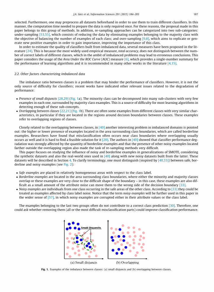
� Presence of small disjuncts [28,29] (Fig. 1a). The minority class can be decomposed into many sub-clusters with very fewexamples in each one, surrounded by majority class examples. This is a source of difficulty for most learning algorithms indetecting enough of these sub-concepts.� Overlapping between classes [22,21] (Fig. 1b). There are often some examples from different classes with very similar char-

acteristics, in particular if they are located in the regions around decision boundaries between classes. These examplesrefer to overlapping regions of classes.

Closely related to the overlapping between classes, in [40] another interesting problem in imbalanced domains is pointedout: the higher or lower presence of examples located in the area surrounding class boundaries, which are called borderlineexamples. Researchers have found that misclassification often occurs near class boundaries where overlapping usuallyoccurs as well and it is hard to find a feasible solution for it [20]. The authors in [40] showed that classifier performance deg-radation was strongly affected by the quantity of borderline examples and that the presence of other noisy examples locatedfarther outside the overlapping region also made the task of re-sampling methods very difficult.

This paper focuses on studying the influence of noisy and borderline examples in generalizations of SMOTE, consideringthe synthetic datasets and also the real-world ones used in [40] along with new noisy datasets built from the latter. Thesedatasets will be described in Section 4. To clarify terminology, one must distinguish (inspired by [40,33]) between safe, bor-derline and noisy examples (see Fig. 2):

� Safe examples are placed in relatively homogeneous areas with respect to the class label.� Borderline examples are located in the area surrounding class boundaries, where either the minority and majority classes

overlap or these examples are very close to the difficult shape of the boundary – in this case, these examples are also dif-ficult as a small amount of the attribute noise can move them to the wrong side of the decision boundary [33].� Noisy examples are individuals from one class occurring in the safe areas of the other class. According to [33] they could be

treated as examples affected by class label noise. Notice that the term noisy examples will be further used in this paper inthe wider sense of [57], in which noisy examples are corrupted either in their attribute values or the class label.

The examples belonging to the last two groups often do not contribute to a correct class prediction [30]. Therefore, onecould ask whether removing them (all or the most difficult misclassification parts) could improve classification performance.

Fig. 1. Examples of the imbalance between classes: (a) small disjuncts and (b) overlapping between classes.

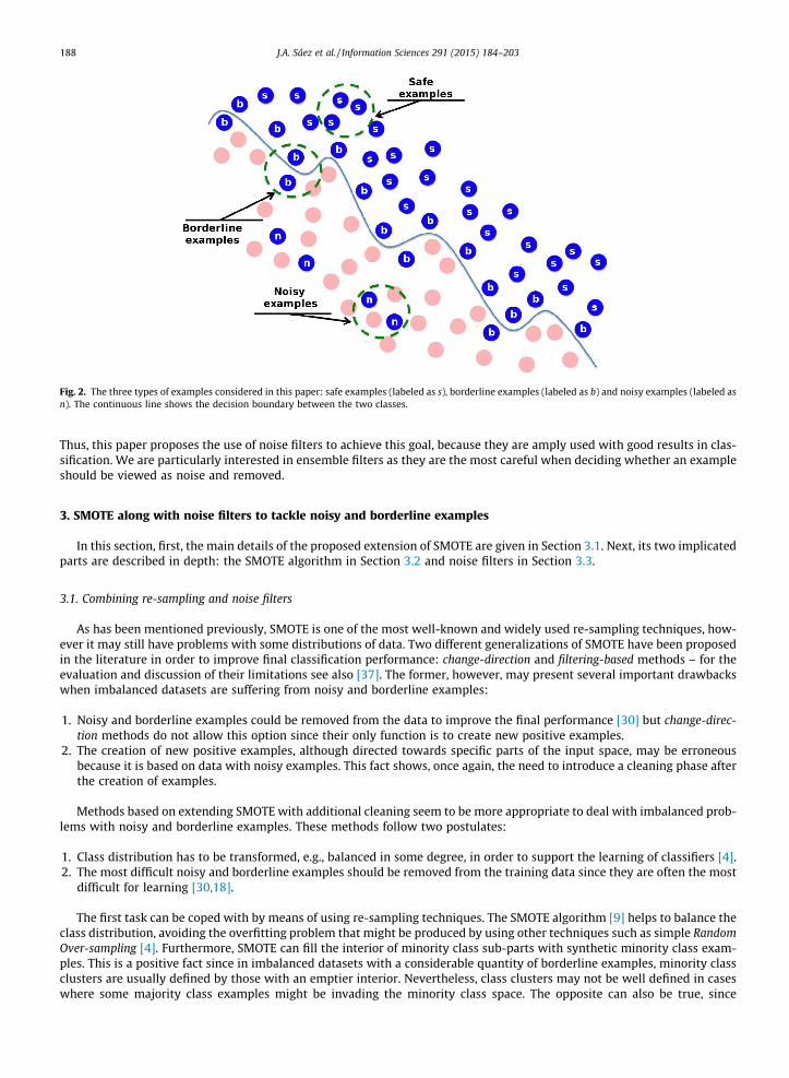
Fig. 2. The three types of examples considered in this paper: safe examples (labeled as s), borderline examples (labeled as b) and noisy examples (labeled asn). The continuous line shows the decision boundary between the two classes.


Thus, this paper proposes the use of noise filters to achieve this goal, because they are amply used with good results in clas-sification. We are particularly interested in ensemble filters as they are the most careful when deciding whether an exampleshould be viewed as noise and removed.

3. SMOTE along with noise filters to tackle noisy and borderline examples

In this section, first, the main details of the proposed extension of SMOTE are given in Section 3.1. Next, its two implicatedparts are described in depth: the SMOTE algorithm in Section 3.2 and noise filters in Section 3.3.

3.1. Combining re-sampling and noise filters

As has been mentioned previously, SMOTE is one of the most well-known and widely used re-sampling techniques, how-ever it may still have problems with some distributions of data. Two different generalizations of SMOTE have been proposedin the literature in order to improve final classification performance: change-direction and filtering-based methods – for theevaluation and discussion of their limitations see also [37]. The former, however, may present several important drawbackswhen imbalanced datasets are suffering from noisy and borderline examples:

1. Noisy and borderline examples could be removed from the data to improve the final performance [30] but change-direc-tion methods do not allow this option since their only function is to create new positive examples.

2. The creation of new positive examples, although directed towards specific parts of the input space, may be erroneousbecause it is based on data with noisy examples. This fact shows, once again, the need to introduce a cleaning phase afterthe creation of examples.

Methods based on extending SMOTE with additional cleaning seem to be more appropriate to deal with imbalanced prob-lems with noisy and borderline examples. These methods follow two postulates:

1. Class distribution has to be transformed, e.g., balanced in some degree, in order to support the learning of classifiers [4].2. The most difficult noisy and borderline examples should be removed from the training data since they are often the most

difficult for learning [30,18].

The first task can be coped with by means of using re-sampling techniques. The SMOTE algorithm [9] helps to balance theclass distribution, avoiding the overfitting problem that might be produced by using other techniques such as simple RandomOver-sampling [4]. Furthermore, SMOTE can fill the interior of minority class sub-parts with synthetic minority class exam-ples. This is a positive fact since in imbalanced datasets with a considerable quantity of borderline examples, minority classclusters are usually defined by those with an emptier interior. Nevertheless, class clusters may not be well defined in caseswhere some majority class examples might be invading the minority class space. The opposite can also be true, since


interpolating minority class examples can expand the minority class clusters, introducing artificial minority class examplestoo deeply into the majority class space. This additional minority noise is also caused by the blind over-generalization ofSMOTE-based techniques of looking for nearest neighbors from the minority class only. Both situations could introduce addi-tional noise into datasets.

The aforementioned problems are already well known. They have been tackled by combining SMOTE with an additionalstep of under-sampling, e.g., with the ENN filtering [55], which aims to remove mislabeled data from the training data afterthe usage of SMOTE. However, these methods do not perform this task as well as they should in all cases.

The second task requires specific and more powerful methods designed to eliminate mislabeled examples when datasetshave a considerable number of such examples. A group of methods that address this problem is ensemble-based noise filters[18,7,54]. This paper proposes the extension of SMOTE with one of these filters: the IPF filter [32], which will be responsiblefor removing noisy examples originally present in the dataset and also those created by SMOTE. Besides this, IPF cleans upclass boundaries, making them more regular and facilitating in this way the posterior learning phase [18].

These two techniques (SMOTE and IPF) must be applied to the imbalanced dataset in the correct order in order to obtainreasonable final results: SMOTE in the first place and then the IPF noise filter. This is due to IPF being designed to deal withstandard classification datasets. Its application over an imbalanced dataset before the usage of SMOTE (which balances thedistribution of classes) may carry the risk of removing all the examples from the minority class, which may be seen as noisyexamples because they are underrepresented in the dataset. In short, as a summary and justification of this approach, it isclaimed that:

1. The SMOTE algorithm fulfills a dual function: it balances the class distribution and it helps to fill in the interior of sub-parts of the minority class.

2. The IPF filter removes the noisy examples originally present in the dataset and also those created by SMOTE. Besides this,IPF cleans up the boundaries of the classes, making them more regular.

Note that the scheme proposed (SMOTE–IPF) enables one to replace SMOTE with any of its modifications, in particular,the change-direction generalizations. However, in this paper we prefer to use the basic version of SMOTE because it is con-sistent with earlier research on the usage of filtering techniques and facilitates the comparison with them. The usage of IPFmay also disturb the effects of the earlier modifications of examples by the change-direction methods. Moreover, some ofthese methods strongly focus on the over-sampling of concrete regions of the original data. For example, Borderline-SMOTEmay over-strength the boundary zone, which will be problematic for studying data with many noisy and borderlineexamples.

3.2. The synthetic minority over-sampling technique

SMOTE [9], introduced by Chawla and co-authors, is now one of the most popular over-sampling methods. In thisapproach, the positive class is over-sampled by taking each minority class example and introducing synthetic examplesalong the line segments joining any/all of the k minority class nearest neighbors. In order to find these neighbors in the spaceof numerical and nominal attributes, the HVDM metric is applied [56]. Depending on the amount of oversampling required,neighbors from the k nearest neighbors are randomly chosen. Analyzing the current literature on the usage of SMOTE, onecan notice that k ¼ 5 neighbors is usually chosen. This procedure of building a local neighborhood is also often applied inother resampling methods, such as SPIDER. Although one could ask a more general question by tuning a particular k valuedepending on the given data characteristics, we decided to use one value k ¼ 5 to be more consistent with other relatedworks on SMOTE and its generalizations since they were compared using the same data sets as we have chosen for our study.Taking the same motivations to be consistent with related works, we tune the oversampling amount to balance both classesto 50%.

Synthetic examples are generated in the following way. Take the difference between the feature vector (sample) underconsideration and its nearest neighbor. Multiply this difference by a random number between 0 and 1, and add it to the fea-ture vector under consideration. This causes the selection of a random point along the line segment between two specificfeatures. This approach effectively forces the decision region of the minority class to become more general.

3.3. Noise filters

Noise filters are preprocessing mechanisms designed to detect and eliminate noisy examples in the training set[55,7,32,44]. The result of noise elimination in preprocessing is a reduced training set which is then used as an input to amachine learning algorithm.

Some of these filters are based on the computation of different measures over the training data. For instance, the methodproposed in [18] is based on the observation that the elimination of noisy examples reduces the Complexity of the Least Com-plex Correct Hypothesis value of the training set.

In addition, there are many other noise filters based on the usage of ensembles. In [7], multiple classifiers belonging todifferent learning paradigms were built and trained from a possibly corrupted dataset and then used to identify mislabeleddata, which is characterized as the examples that are incorrectly classified by the multiple classifiers. Similar techniques


have been widely developed considering the building of several classifiers with the same learning algorithm [17,54]. Insteadof using multiple classifiers learned from the same training set, in [17] a Classification Filter (CF) approach is suggested, inwhich the training set is partitioned into n subsets, then a set of classifiers is trained from the union of any n� 1 subsets;those classifiers are used to classify the examples in the excluded subset, eliminating the examples that are incorrectlyclassified.

From our knowledge and preliminary, earlier experiments performed with different ensemble-based filters, e.g., theEnsemble Filter (EF) [7], the Cross-Validated Committees Filter (CVCF) [54], CF and others, the notable good behavior of the Iter-ative-Partitioning Filter [32] when detecting noisy examples must be pointed out. IPF has characteristics which differentiate itfrom most of the noise filters and may provide the reasons why it performs better than them – they will be analyzed anddiscussed in Section 6.

IPF removes noisy examples in multiple iterations until a stopping criterion is reached. The iterative process stops when,for a number of consecutive iterations k, the number of identified noisy examples in each of these iterations is less than apercentage p of the size of the original training dataset. Initially, the method starts with a set of noisy examples A ¼ ;.The basic steps of each iteration as follows:

1. Split the current training dataset E into n equal sized subsets.2. Build a classifier with the C4.5 algorithm over each of these n subsets and use them to evaluate the whole current training

dataset E.3. Add to A the noisy examples identified in E using a voting scheme (consensus or majority).4. Remove the noisy examples: E E n A.

Two voting schemes can be used to identify noisy examples: consensus and majority. The former removes an example if itis misclassified by all the classifiers, whereas the latter removes an example if it is misclassified by more than half of theclassifiers.

The parameter setup for the implementation of IPF used in this work has been determined experimentally in order tobetter fit it to the characteristics of imbalanced datasets with noisy and borderline examples once they have been prepro-cessed with SMOTE. More precisely, the majority scheme is used to identify the noisy examples, n ¼ 9 partitions with ran-dom examples in each one are created and k ¼ 3 iterations for the stop criterion and p ¼ 1% of removed examples areconsidered. This parameter setup is based on a study of the influence of each parameter on the results – the justificationof each parameter value and its influence is given in Section 6.3.

4. Experimental framework

In this section, the details of the experimental study developed in this paper are presented. First, in Section 4.1, wedescribe how the synthetic imbalanced datasets with borderline examples were built. Then, the real-world datasets andthe noise introduction processes are presented in Section 4.2. In Section 4.3 the preprocessing techniques considered in thiswork are briefly described. Finally, in Section 4.4, the methodology of the analysis carried out is described.

4.1. Synthetic imbalanced datasets with borderline examples

This paper uses the family of synthetic datasets used in prior research on the role of borderline examples [40]. These datawere created following other experimental studies of small disjuncts [28,29] and overlapping between classes [21]. However,these studies were focused on studying single factors and very simple (lines and rectangles) shapes of decision boundaries.Thus, the authors of [40] created more complex data affected by many factors, including borderline examples. Many datasetswith different configurations were generated by special software and evaluated; for more details see [46]. In this paper weconsider these configurations of datasets which were the basis for the previous analysis of the role of borderline examplesfor different basic classifiers, such as C4.5, and re-sampling methods [40]. These datasets are briefly characterized below:

1. Number of classes and attributes. This work focuses on binary classification problems (the minority versus the majorityclass) with examples randomly and uniformly distributed in the two-dimensional real-value space.

2. Number of examples and imbalance ratios. Multiple datasets with two different numbers of examples and imbalance ratiosare considered: datasets with 600 examples and IR ¼ 5 and datasets with 800 examples and IR ¼ 7. The values of theparameters resulted from the assumption of having at least 20 examples for the subpart of the decomposed minorityclass. Smaller cardinalities led to unstable results [46].

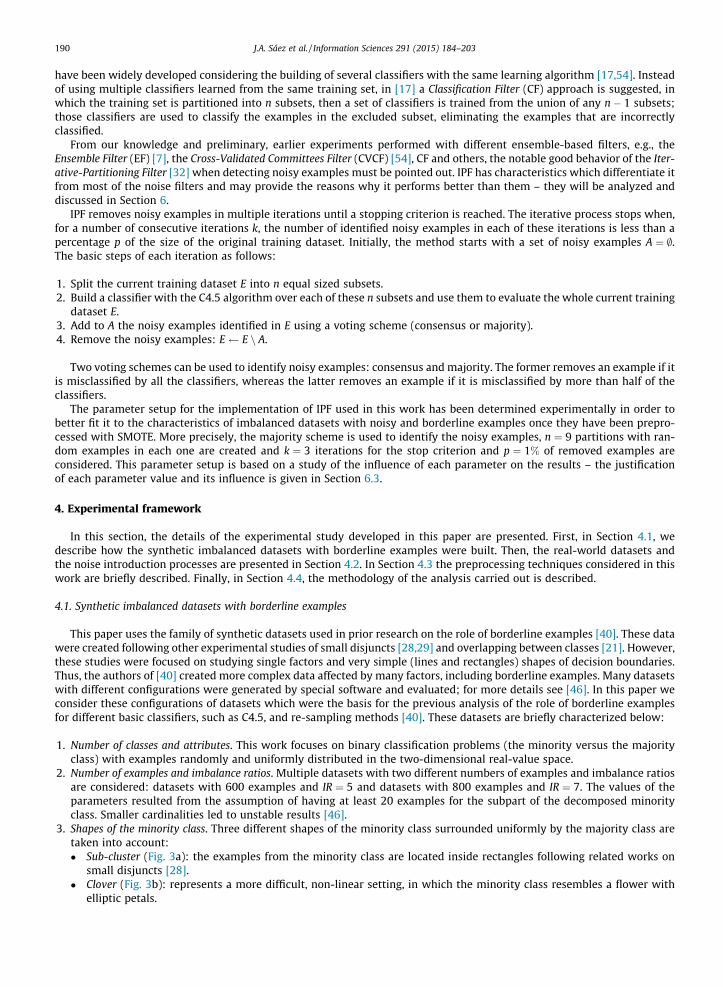
3. Shapes of the minority class. Three different shapes of the minority class surrounded uniformly by the majority class aretaken into account:� Sub-cluster (Fig. 3a): the examples from the minority class are located inside rectangles following related works on

small disjuncts [28].� Clover (Fig. 3b): represents a more difficult, non-linear setting, in which the minority class resembles a flower with

elliptic petals.

(a) Sub-cluster. (b) Clover. (c) Paw.

Fig. 3. Shapes of the minority class.


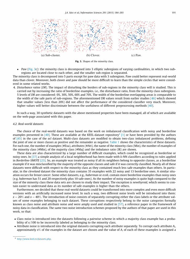
� Paw (Fig. 3c): the minority class is decomposed into 3 elliptic subregions of varying cardinalities, in which two sub-regions are located close to each other, and the smaller sub-region is separated.

The minority class is decomposed into 5 parts except for paw data with 3 subregions. Paw could better represent real-worlddata than clover. Moreover, both clover and paw should be more difficult to learn than the simple circles that were consid-ered in some related works.4. Disturbance ratios (DR). The impact of disturbing the borders of sub-regions in the minority class will is studied. This is

carried out by increasing the ratio of borderline examples, i.e., the disturbance ratio, from the minority class subregions.5 levels of DR are considered: 0%, 30%, 50%, 60% and 70%. The width of the borderline overlapping areas is comparable tothe width of the safe parts of sub-regions. The aforementioned DR values result from earlier studies [46] which showedthat smaller values (less than 20%) did not affect the performance of the considered classifier very much. Moreover,higher values will better discriminate between the usefulness of different preprocessing methods [40].

In such a way, 30 synthetic datasets with the above mentioned properties have been managed, all of which are availableon the web-page associated with this paper.

4.2. Real-world datasets

The choice of the real-world datasets was based on the work on imbalanced classification with noisy and borderlineexamples presented in [40]. These are available at the KEEL-dataset repository2 [1] or have been provided by the authorsof [45] in the case of the acl dataset. Multi-class datasets are modified to obtain two-class imbalanced problems, definingthe joint of one or more classes as positive and the remainder as negative. Table 1 shows the characteristics of these datasets.For each one, the number of examples (#Exa), attributes (#Att), the name of the minority class (Min), the number of examples ofthe minority class (#Min), of the majority class (#Maj) and the imbalance ratio (IR) are shown.

These data are also characterized by a large number of difficult examples, which could be recognized as borderline ornoisy ones. In [37] a simple analysis of a local neighborhood has been made with k-NN classifiers according to rules appliedin Borderline-SMOTE [23]. So, an example was treated as noisy if all its neighbors belong to opposite classes, as a borderlineexample if it was misclassified by the majority of the opposite classes and safe if it was correctly classified. Nearly all of thesedatasets were difficult with respect to the minority class as they contained much less safe examples than others. In partic-ular, in the cleveland dataset the minority class contains 35 examples with 22 noisy and 13 borderline ones. A similar situ-ation occurs for breast cancer. Some other datasets, e.g., haberman or ecoli, contain more borderline examples than noisy ones(e.g. haberman has 51 and 20 respectively plus 10 safe ones). As the number of noisy examples is quite high compared to thesize of the minority class these data sets are chosen to study their impact. The exception is newthyroid, which seems to con-tain easier to understand data as its number of safe examples is higher than the others.

Furthermore, we decided that these real-world datasets could be transformed into more complex and even more difficultversions with an artificially increased noise level. In such a way, two different noise levels will be introduced into them:x ¼ 20% and x ¼ 40%. The introduction of noise consists of separately corrupting either the class labels or the attribute val-ues of some examples belonging to each dataset. These corruptions respectively belong to the noise categories formallyknown as class noise and attribute noise and were amply used and studied in [57], a reference paper in the framework ofnoisy data in classification. The same two noise introduction schemes proposed by the authors of that paper are used in thiswork, so that:

� Class noise is introduced into the datasets following a pairwise scheme in which a majority class example has a proba-bility of x=100 to be incorrectly labeled as belonging to the minority class.� Attribute noise is introduced into the original datasets corrupting each attribute separately. To corrupt each attribute Ai,

approximately x% of the examples in the dataset are chosen and the value of Ai of each of these examples is assigned a

2 http://www.keel.es/datasets.php.

http://www.keel.es/datasets.php

Table 1Characteristics of the real-world datasets.

Dataset #Exa #Att Min #Min #Maj IR

acl 140 6 with knee injury 40 100 2.5breast 286 9 recurrence-events 85 201 2.36bupa 345 6 sick 145 200 1.38cleveland 303 13 positive 35 268 7.66ecoli 336 7 imU 35 301 8.60haberman 306 3 died 81 225 2.78hepatitis 155 19 die 32 123 3.84newthyroid 215 5 hyper 35 180 5.14pima 768 8 positive 268 500 1.87


random value between the minimum and maximum of the domain of that attribute following a uniform distribution (if Ai

is numerical), or choosing a random value of the domain (if Ai is nominal).

The performance estimation of each classifier for each of these real-world datasets, and also for the synthetic ones, isobtained by means of 5 runs of a stratified 5-fold cross-validation and their results are averaged. Dividing the dataset into5 folds is considered in order to dispose of a sufficient quantity of minority class examples in the test partitions. In this way,test partition examples are more representative of the underlying knowledge and meaningful performance results can beobtained.

4.3. Re-sampling techniques for comparison

Different re-sampling techniques to adjust the class distribution in the training data based on generalizations of SMOTEare studied in this paper. The usefulness of a new SMOTE extension is studied in a comprehensive comparative study withother, related versions of SMOTE, in particular the best known representations of change-direction and filtering-based meth-ods. Table 2 shows the SMOTE-based methods considered in this study – a wider description of such methods is found on theweb-page associated with this paper.

Note that SMOTE-TL and SMOTE-ENN are approaches based on extending SMOTE with an additional filtering(filtering-based methods), whereas SL-SMOTE, B1-SMOTE and B2-SMOTE are approaches based on directing the creation ofthe positive examples (change-direction methods).

4.4. Analysis methodology

In order to check the suitability of the proposed extension of SMOTE versus the other re-sampling techniques when deal-ing with imbalanced datasets with noisy and borderline examples, the experiments are divided into three differentiatedparts depending on the type of datasets considered in each one: synthetic, real-world and noisy modified real-worlddatasets.

The effect of the aforementioned preprocessing techniques will be analyzed comparing the AUC for each dataset obtainedwith C4.5 [41], which has been used in many other works in imbalanced classification, in particular concerning SMOTE[47,48]. Furthermore, it is known to be more sensitive to different factors of imbalanced data than, e.g., SVM [13] and is oftenused inside the ensembles. The standard parameters along with a post-pruning have been considered for the executions.

For each of the three types of datasets, the AUC results obtained by C4.5 for our approach against (i) not applyingpreprocessing and applying SMOTE alone, (ii) the other filtering-based methods (SMOTE-ENN and SMOTE-TL) and (iii) thechange-direction methods (B1-SMOTE, B2-SMOTE and SL-SMOTE) will be separately compared. We have separately studiedthe differences between our proposal and the filtering-based and change-direction methods for two main reasons. First, theseparation is motivated by the different nature of the methods of both groups that share common characteristics, whichallow us to independently obtain conclusions with each kind of method. On the other hand, performing a multiple statisticalcomparison usually requires a much higher quantity of datasets to detect significant differences when the number of com-parison methods increases. Multiple statistical comparisons are then limited by the number of datasets, and the comparison

Table 2Re-sampling techniques considered.

Method Reference Method Reference

SMOTE [9] SL-SMOTE [8]SMOTE-TL [4] B1-SMOTE [23]SMOTE-ENN [4] B2-SMOTE [23]


grouping the two types of methods (filtering-based and change-direction) can only be performed if a much higher quantityof datasets than the one considered in this paper is available for study.

Additionally, statistical comparisons in each of these cases will be also performed. Wilcoxon’s signed ranks statistical test[14] will be applied to compare SMOTE–IPF with no preprocessing and the usage of SMOTE alone. This is a nonparametricpairwise test that aims to detect significant differences between two sample means; that is, the behavior of the two algo-rithms involved in each comparison. The results of the two methods involved in the comparison over all the datasets willbe compared using Wilcoxon’s test and the p-values associated with these comparisons will be obtained. The p-valuerepresents the lowest level of significance of a hypothesis that results in a rejection and it allows one to know both whethertwo algorithms are significantly different and the degree of their difference.

Regarding the comparison between our approach and the other re-sampling techniques (either filtering-based or change-direction methods), the aligned Friedman’s procedure [19] will be used. This is an advanced nonparametric test for perform-ing multiple comparisons, which improves the classic Friedman test. The Friedman test is based on sets of ranks, one set foreach data set; and the performances of the algorithms analyzed are ranked separately for each data set. Such a rankingscheme allows for intra-set comparisons only, since inter-set comparisons are not meaningful. When the number of algo-rithms for comparison is small, this may pose a disadvantage. In such cases, comparability among data sets is desirableand we can employ the method of aligned ranks [26]. Because of this, we will use the aligned Friedman’s test to computethe set of ranks that represent the effectiveness associated with each algorithm and the p-value related to the significanceof the differences found by this test. In addition, the adjusted p-value with Hochberg’s test [25] will be computed. Moreinformation about these tests and other statistical procedures can be found at http://sci2s.ugr.es/sicidm/.

We will consider a difference to be significant if the p-value obtained is lower than 0.1 [14,19] – even though p-valuesslightly higher than 0.1 might be also showing important differences.

5. Evaluation of re-sampling methods with noisy and borderline examples

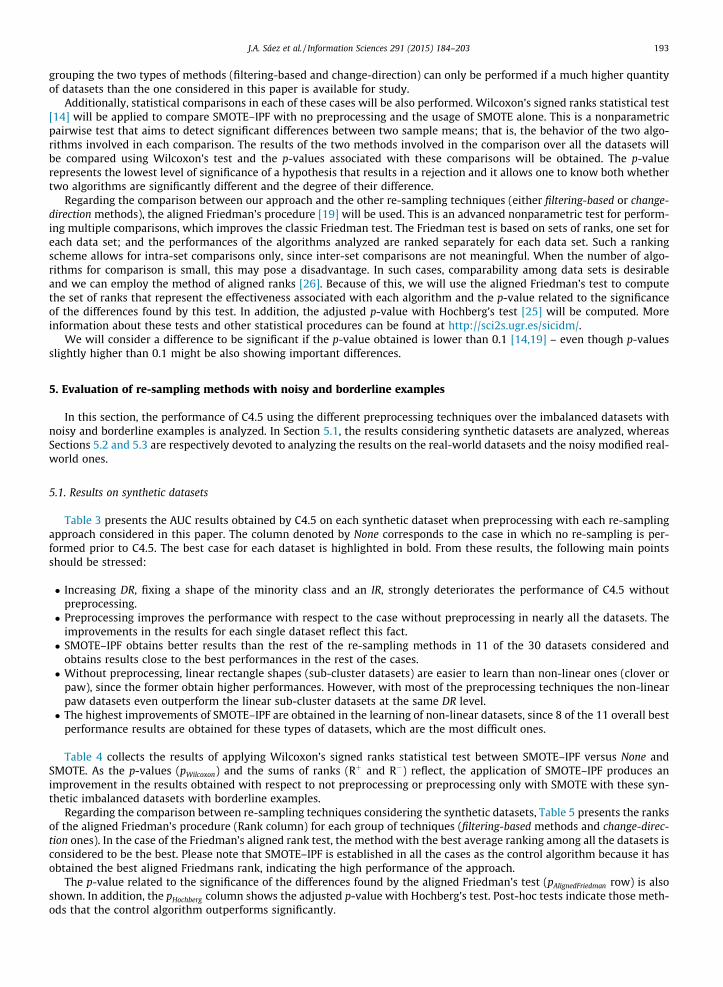
In this section, the performance of C4.5 using the different preprocessing techniques over the imbalanced datasets withnoisy and borderline examples is analyzed. In Section 5.1, the results considering synthetic datasets are analyzed, whereasSections 5.2 and 5.3 are respectively devoted to analyzing the results on the real-world datasets and the noisy modified real-world ones.

5.1. Results on synthetic datasets

Table 3 presents the AUC results obtained by C4.5 on each synthetic dataset when preprocessing with each re-samplingapproach considered in this paper. The column denoted by None corresponds to the case in which no re-sampling is per-formed prior to C4.5. The best case for each dataset is highlighted in bold. From these results, the following main pointsshould be stressed:

� Increasing DR, fixing a shape of the minority class and an IR, strongly deteriorates the performance of C4.5 withoutpreprocessing.� Preprocessing improves the performance with respect to the case without preprocessing in nearly all the datasets. The

improvements in the results for each single dataset reflect this fact.� SMOTE–IPF obtains better results than the rest of the re-sampling methods in 11 of the 30 datasets considered and

obtains results close to the best performances in the rest of the cases.� Without preprocessing, linear rectangle shapes (sub-cluster datasets) are easier to learn than non-linear ones (clover or

paw), since the former obtain higher performances. However, with most of the preprocessing techniques the non-linearpaw datasets even outperform the linear sub-cluster datasets at the same DR level.� The highest improvements of SMOTE–IPF are obtained in the learning of non-linear datasets, since 8 of the 11 overall best

performance results are obtained for these types of datasets, which are the most difficult ones.

Table 4 collects the results of applying Wilcoxon’s signed ranks statistical test between SMOTE–IPF versus None andSMOTE. As the p-values (pWilcoxon) and the sums of ranks (Rþ and R�) reflect, the application of SMOTE–IPF produces animprovement in the results obtained with respect to not preprocessing or preprocessing only with SMOTE with these syn-thetic imbalanced datasets with borderline examples.

Regarding the comparison between re-sampling techniques considering the synthetic datasets, Table 5 presents the ranksof the aligned Friedman’s procedure (Rank column) for each group of techniques (filtering-based methods and change-direc-tion ones). In the case of the Friedman’s aligned rank test, the method with the best average ranking among all the datasets isconsidered to be the best. Please note that SMOTE–IPF is established in all the cases as the control algorithm because it hasobtained the best aligned Friedmans rank, indicating the high performance of the approach.

The p-value related to the significance of the differences found by the aligned Friedman’s test (pAlignedFriedman row) is alsoshown. In addition, the pHochberg column shows the adjusted p-value with Hochberg’s test. Post-hoc tests indicate those meth-ods that the control algorithm outperforms significantly.

http://sci2s.ugr.es/sicidm/

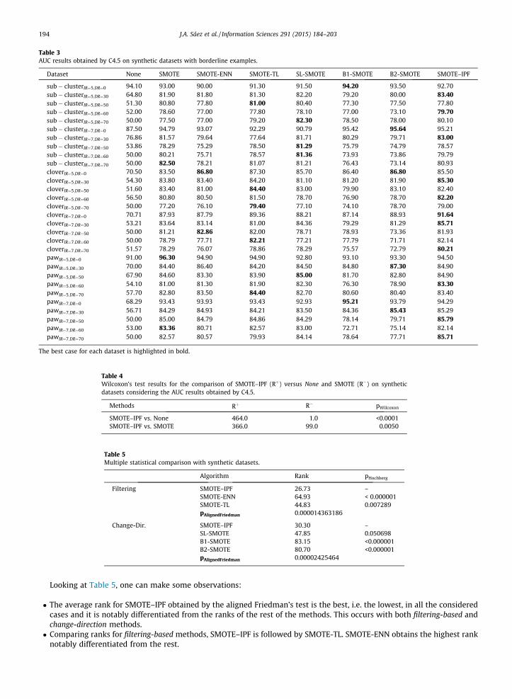
Table 3AUC results obtained by C4.5 on synthetic datasets with borderline examples.

Dataset None SMOTE SMOTE-ENN SMOTE-TL SL-SMOTE B1-SMOTE B2-SMOTE SMOTE–IPF

sub� clusterIR¼5;DR¼0 94.10 93.00 90.00 91.30 91.50 94.20 93.50 92.70sub� clusterIR¼5;DR¼30 64.80 81.90 81.80 81.30 82.20 79.20 80.00 83.40sub� clusterIR¼5;DR¼50 51.30 80.80 77.80 81.00 80.40 77.30 77.50 77.80sub� clusterIR¼5;DR¼60 52.00 78.60 77.00 77.80 78.10 77.00 73.10 79.70sub� clusterIR¼5;DR¼70 50.00 77.50 77.00 79.20 82.30 78.50 78.00 80.10sub� clusterIR¼7;DR¼0 87.50 94.79 93.07 92.29 90.79 95.42 95.64 95.21sub� clusterIR¼7;DR¼30 76.86 81.57 79.64 77.64 81.71 80.29 79.71 83.00sub� clusterIR¼7;DR¼50 53.86 78.29 75.29 78.50 81.29 75.79 74.79 78.57sub� clusterIR¼7;DR¼60 50.00 80.21 75.71 78.57 81.36 73.93 73.86 79.79sub� clusterIR¼7;DR¼70 50.00 82.50 78.21 81.07 81.21 76.43 73.14 80.93cloverIR¼5;DR¼0 70.50 83.50 86.80 87.30 85.70 86.40 86.80 85.50cloverIR¼5;DR¼30 54.30 83.80 83.40 84.20 81.10 81.20 81.90 85.30cloverIR¼5;DR¼50 51.60 83.40 81.00 84.40 83.00 79.90 83.10 82.40cloverIR¼5;DR¼60 56.50 80.80 80.50 81.50 78.70 76.90 78.70 82.20cloverIR¼5;DR¼70 50.00 77.20 76.10 79.40 77.10 74.10 78.70 79.00cloverIR¼7;DR¼0 70.71 87.93 87.79 89.36 88.21 87.14 88.93 91.64cloverIR¼7;DR¼30 53.21 83.64 83.14 81.00 84.36 79.29 81.29 85.71cloverIR¼7;DR¼50 50.00 81.21 82.86 82.00 78.71 78.93 73.36 81.93cloverIR¼7;DR¼60 50.00 78.79 77.71 82.21 77.21 77.79 71.71 82.14cloverIR¼7;DR¼70 51.57 78.29 76.07 78.86 78.29 75.57 72.79 80.21pawIR¼5;DR¼0 91.00 96.30 94.90 94.90 92.80 93.10 93.30 94.50pawIR¼5;DR¼30 70.00 84.40 86.40 84.20 84.50 84.80 87.30 84.90pawIR¼5;DR¼50 67.90 84.60 83.30 83.90 85.00 81.70 82.80 84.90pawIR¼5;DR¼60 54.10 81.00 81.30 81.90 82.30 76.30 78.90 83.30pawIR¼5;DR¼70 57.70 82.80 83.50 84.40 82.70 80.60 80.40 83.40pawIR¼7;DR¼0 68.29 93.43 93.93 93.43 92.93 95.21 93.79 94.29pawIR¼7;DR¼30 56.71 84.29 84.93 84.21 83.50 84.36 85.43 85.29pawIR¼7;DR¼50 50.00 85.00 84.79 84.86 84.29 78.14 79.71 85.79pawIR¼7;DR¼60 53.00 83.36 80.71 82.57 83.00 72.71 75.14 82.14pawIR¼7;DR¼70 50.00 82.57 80.57 79.93 84.14 78.64 77.71 85.71

The best case for each dataset is highlighted in bold.

Table 4Wilcoxon’s test results for the comparison of SMOTE–IPF (Rþ) versus None and SMOTE (R�) on syntheticdatasets considering the AUC results obtained by C4.5.

Methods Rþ R� pWilcoxon

SMOTE–IPF vs. None 464.0 1.0 <0.0001SMOTE–IPF vs. SMOTE 366.0 99.0 0.0050

Table 5Multiple statistical comparison with synthetic datasets.

Algorithm Rank pHochberg

Filtering SMOTE–IPF 26.73 –SMOTE-ENN 64.93 < 0.000001SMOTE-TL 44.83 0.007289pAlignedFriedman 0.000014363186

Change-Dir. SMOTE–IPF 30.30 –SL-SMOTE 47.85 0.050698B1-SMOTE 83.15 <0.000001B2-SMOTE 80.70 <0.000001pAlignedFriedman 0.00002425464


Looking at Table 5, one can make some observations:

� The average rank for SMOTE–IPF obtained by the aligned Friedman’s test is the best, i.e. the lowest, in all the consideredcases and it is notably differentiated from the ranks of the rest of the methods. This occurs with both filtering-based andchange-direction methods.� Comparing ranks for filtering-based methods, SMOTE–IPF is followed by SMOTE-TL. SMOTE-ENN obtains the highest rank

notably differentiated from the rest.


� Among the change-direction methods, SL-SMOTE outperforms the ranks of B1-SMOTE and B2-SMOTE, which are quitesimilar.� The p-values of the aligned Friedman’s test are very low in all the scenarios, which shows a great significance in the dif-

ferences found.� The adjusted p-values by Hochberg’s test are very low in all comparisons.

From the results of Tables 3–5, one can conclude that SMOTE–IPF performs better than other SMOTE versions when dealingwith the synthetic imbalanced datasets built with borderline examples, particularly in those with non-linear shapes of theminority class. All the statistical tests also clearly show the statistical significance of this better performance of SMOTE–IPF.

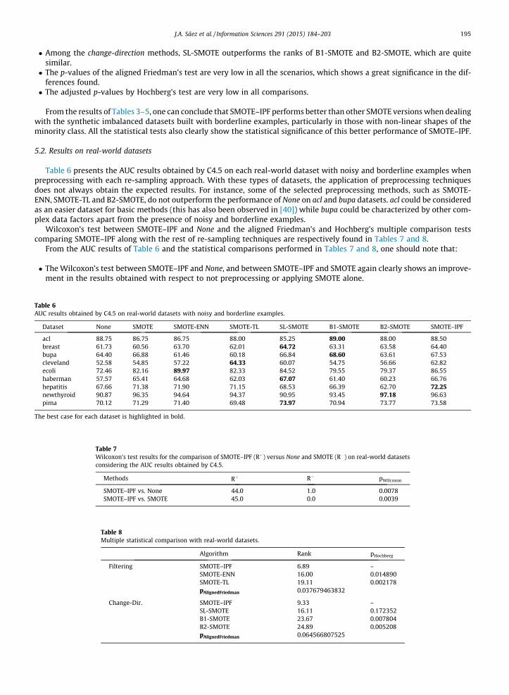
5.2. Results on real-world datasets

Table 6 presents the AUC results obtained by C4.5 on each real-world dataset with noisy and borderline examples whenpreprocessing with each re-sampling approach. With these types of datasets, the application of preprocessing techniquesdoes not always obtain the expected results. For instance, some of the selected preprocessing methods, such as SMOTE-ENN, SMOTE-TL and B2-SMOTE, do not outperform the performance of None on acl and bupa datasets. acl could be consideredas an easier dataset for basic methods (this has also been observed in [40]) while bupa could be characterized by other com-plex data factors apart from the presence of noisy and borderline examples.

Wilcoxon’s test between SMOTE–IPF and None and the aligned Friedman’s and Hochberg’s multiple comparison testscomparing SMOTE–IPF along with the rest of re-sampling techniques are respectively found in Tables 7 and 8.

From the AUC results of Table 6 and the statistical comparisons performed in Tables 7 and 8, one should note that:

� The Wilcoxon’s test between SMOTE–IPF and None, and between SMOTE–IPF and SMOTE again clearly shows an improve-ment in the results obtained with respect to not preprocessing or applying SMOTE alone.

Table 6AUC results obtained by C4.5 on real-world datasets with noisy and borderline examples.


acl 88.75 86.75 86.75 88.00 85.25 89.00 88.00 88.50breast 61.73 60.56 63.70 62.01 64.72 63.31 63.58 64.40bupa 64.40 66.88 61.46 60.18 66.84 68.60 63.61 67.53cleveland 52.58 54.85 57.22 64.33 60.07 54.75 56.66 62.82ecoli 72.46 82.16 89.97 82.33 84.52 79.55 79.37 86.55haberman 57.57 65.41 64.68 62.03 67.07 61.40 60.23 66.76hepatitis 67.66 71.38 71.90 71.15 68.53 66.39 62.70 72.25newthyroid 90.87 96.35 94.64 94.37 90.95 93.45 97.18 96.63pima 70.12 71.29 71.40 69.48 73.97 70.94 73.77 73.58


Table 7Wilcoxon’s test results for the comparison of SMOTE–IPF (Rþ) versus None and SMOTE (R�) on real-world datasetsconsidering the AUC results obtained by C4.5.

Methods Rþ R� pWilcoxon

SMOTE–IPF vs. None 44.0 1.0 0.0078SMOTE–IPF vs. SMOTE 45.0 0.0 0.0039

Table 8Multiple statistical comparison with real-world datasets.

Algorithm Rank pHochberg

Filtering SMOTE–IPF 6.89 –SMOTE-ENN 16.00 0.014890SMOTE-TL 19.11 0.002178pAlignedFriedman 0.037679463832

Change-Dir. SMOTE–IPF 9.33 –SL-SMOTE 16.11 0.172352B1-SMOTE 23.67 0.007804B2-SMOTE 24.89 0.005208pAlignedFriedman 0.064566807525


� SMOTE–IPF only obtains the best results on one single dataset (hepatitis) considering all the preprocessing methods.However, the Friedman’s rank of SMOTE–IPF is clearly the best result compared with the rest of re-sampling techniquesif the performance of all the datasets is summarized. This shows the great robustness of SMOTE–IPF when applied to thereal-world datasets.� The p-values of the aligned Friedman’s test are very low in all the scenarios, which shows a great significance in the

differences found.� The adjusted p-values by Hochberg’s test are also very low in all comparisons, particularly with the filtering-based meth-

ods, even though with SL-SMOTE the p-value obtained is a little higher. Therefore, the suitability of SMOTE–IPF to addressimbalanced real-world datasets with noisy and borderline examples is statistically shown.

Comparing the results of the synthetic datasets in Table 5 with respect to those of the real-world ones in Table 8, oneobserves that some of the methods that obtain the better Friedman’s ranks on synthetic datasets, such as SMOTE-TL amongthe filtering-based methods, obtain less notable results on real-world ones. The latter data are perhaps more complex thanthe former and they may require more elaborate techniques. SMOTE–IPF remains the best method considering its alignedFriedman’s rank and the Hochberg’s test p-values with both synthetic and real-world datasets.

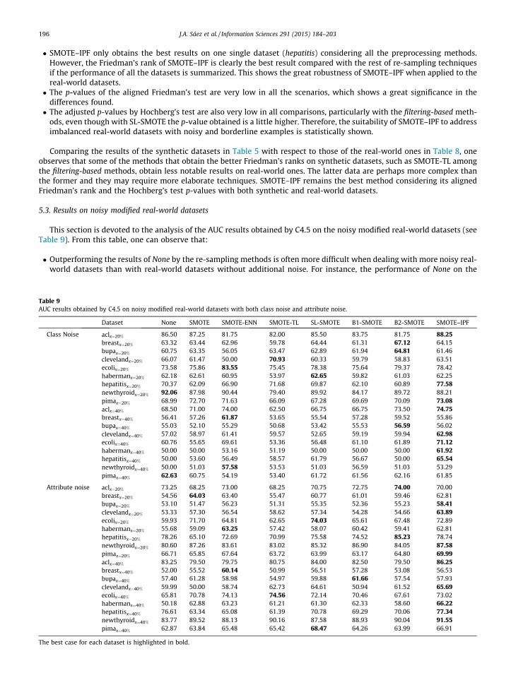
5.3. Results on noisy modified real-world datasets

This section is devoted to the analysis of the AUC results obtained by C4.5 on the noisy modified real-world datasets (seeTable 9). From this table, one can observe that:

� Outperforming the results of None by the re-sampling methods is often more difficult when dealing with more noisy real-world datasets than with real-world datasets without additional noise. For instance, the performance of None on the

Table 9AUC results obtained by C4.5 on noisy modified real-world datasets with both class noise and attribute noise.


Class Noise aclx¼20% 86.50 87.25 81.75 82.00 85.50 83.75 81.75 88.25breastx¼20% 63.32 63.44 62.96 59.78 64.44 61.31 67.12 64.15bupax¼20% 60.75 63.35 56.05 63.47 62.89 61.94 64.81 61.46clevelandx¼20% 66.07 61.47 50.00 70.93 60.33 59.79 58.83 63.51ecolix¼20% 73.58 75.86 83.55 75.45 78.38 75.64 79.37 78.42habermanx¼20% 62.18 62.61 60.95 53.97 62.65 59.82 61.03 62.25hepatitisx¼20% 70.37 62.09 66.90 71.68 69.87 62.10 60.89 77.58newthyroidx¼20% 92.06 87.98 90.44 79.40 89.92 84.17 89.72 88.21pimax¼20% 68.99 72.70 71.63 66.09 67.28 69.69 70.09 73.08aclx¼40% 68.50 71.00 74.00 62.50 66.75 66.75 73.50 74.75breastx¼40% 56.41 57.26 61.87 53.65 55.54 57.28 59.52 55.86bupax¼40% 55.03 52.10 55.29 50.68 53.42 55.53 56.59 56.02clevelandx¼40% 57.02 58.97 61.41 59.57 52.65 59.19 59.94 62.98ecolix¼40% 60.76 55.65 69.61 53.36 56.48 61.10 61.89 71.12habermanx¼40% 50.00 50.00 53.16 51.19 50.00 50.00 50.00 61.92hepatitisx¼40% 50.00 53.60 56.49 58.57 61.79 56.67 50.00 65.54newthyroidx¼40% 50.00 51.03 57.58 53.53 51.03 56.59 51.03 53.29pimax¼40% 62.63 60.75 54.19 53.40 61.72 61.56 62.16 61.85

Attribute noise aclx¼20% 73.25 68.25 73.00 68.25 70.75 72.75 74.00 70.00breastx¼20% 54.56 64.03 63.40 55.47 60.77 61.01 59.46 62.81bupax¼20% 53.10 51.47 56.23 51.31 55.35 52.36 55.23 58.41clevelandx¼20% 53.33 57.30 56.54 58.62 57.34 54.28 54.66 63.89ecolix¼20% 59.93 71.70 64.81 62.65 74.03 65.61 67.48 72.89habermanx¼20% 55.68 59.09 63.25 57.42 58.07 60.42 59.41 62.81hepatitisx¼20% 78.26 65.10 72.69 70.99 75.58 74.52 85.23 78.74newthyroidx¼20% 80.60 87.26 83.61 83.02 85.32 86.90 84.05 87.58pimax¼20% 66.71 65.85 67.64 63.72 63.99 63.17 64.80 69.99aclx¼40% 83.25 79.50 79.75 80.75 84.00 82.50 79.50 86.25breastx¼40% 52.00 55.52 60.14 50.99 56.51 57.28 53.08 56.53bupax¼40% 57.40 61.28 58.98 54.97 59.88 61.66 57.54 57.93clevelandx¼40% 59.99 50.00 58.74 62.73 64.61 50.94 61.52 65.69ecolix¼40% 65.81 70.78 74.13 74.56 72.14 70.46 67.61 73.02habermanx¼40% 50.18 62.88 63.23 61.21 61.30 62.33 58.60 66.22hepatitisx¼40% 76.61 63.34 65.08 61.39 70.78 69.29 70.06 77.34newthyroidx¼40% 83.77 89.52 88.13 90.16 87.58 88.93 90.04 91.55pimax¼40% 62.87 63.84 65.48 65.42 68.47 64.26 63.99 66.91



newthyroidx¼20% and pimax¼40% datasets with class noise are the best results with respect to considering the use ofpreprocessing.� The observation of the best results in each single dataset show that SMOTE–IPF is the best method in 8 of 18 class noise

datasets, whereas it is the best in 9 of 18 attribute noise datasets. SMOTE-ENN and B2-SMOTE are also notable, with eachobtaining 3 of 18 of the best results in class noise datasets and 2 of 18 in attribute noise datasets.

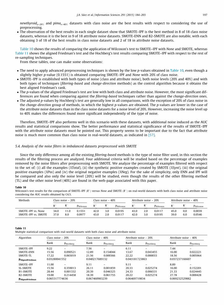
Table 10 shows the results of comparing the application of Wilcoxon’s test to SMOTE–IPF with None and SMOTE, whereasTable 11 shows the aligned Friedman’s test and the Hochberg’s test results comparing SMOTE–IPF with respect to the rest ofre-sampling techniques.

From these tables, one can make some observations:

� The need to apply advanced preprocessing techniques is shown by the low p-values obtained in Table 10, even though aslightly higher p-value (0.1551) is obtained comparing SMOTE–IPF and None with 20% of class noise.� SMOTE–IPF is established with both types of noise (class and attribute noise), both noise levels (20% and 40%) and with

both types of techniques (filtering-based and change-direction methods) as the control algorithm because it obtains thebest aligned Friedman’s rank.� The p-values of the aligned Friedman’s test are low with both class and attribute noise. However, the most significant dif-

ferences are found when comparing against the filtering-based techniques rather than against the change-direction ones.� The adjusted p-values by Hochberg’s test are generally low in all comparisons, with the exception of 20% of class noise in

the change-direction group of methods, in which the highest p-values are obtained. The p-values are lower in the case ofthe attribute noise datasets than in the class noise datasets for a noise level of 20%. However, increasing the noise level upto 40% makes the differences found more significant independently of the type of noise.

Therefore, SMOTE–IPF also performs well in this scenario with these datasets, with additional noise induced as the AUCresults and statistical comparisons show. The better performance and statistical significance of the results of SMOTE–IPFwith the attribute noise datasets must be pointed out. This property seems to be important due to the fact that attributenoise is much more common than class noise in real-world datasets, as indicated in [57].

5.4. Analysis of the noise filters in imbalanced datasets preprocessed with SMOTE

Since the only difference among all the existing filtering-based methods is the type of noise filter used, in this section theresults of the filtering process are analyzed. Four additional criteria will be studied based on the percentage of examplesremoved by the noise filters after preprocessing with SMOTE. We analyze the percentage of examples filtered with respectto the set of: (i) all the examples (%Total), (ii) the synthetic positive examples created by SMOTE (%Synt), (iii) the originalpositive examples (%Pos) and (iv) the original negative examples (%Neg). For the sake of simplicity, only ENN and IPF willbe compared and also only the noise level (20%) will be studied, even though the results of the other filtering method(TL) and the other noise level (40%) are found in the web-page associated with this paper.

Table 10Wilcoxon’s test results for the comparison of SMOTE–IPF ðRþÞ versus None and SMOTE ðR�Þ on real-world datasets with both class noise and attribute noiseconsidering the AUC results obtained by C4.5.

Methods Class noise – 20% Class noise – 40% Attribute noise – 20% Attribute noise – 40%

Rþ R� pWilcoxon Rþ R� pWilcoxon Rþ R� pWilcoxon Rþ R� pWilcoxon

SMOTE–IPF vs. None 34.0 11.0 0.1551 42.0 3.0 0.0195 43.0 2.0 0.0117 45.0 0.0 0.0039SMOTE–IPF vs. SMOTE 37.0 8.0 0.0977 43.0 2.0 0.0117 42.0 3.0 0.0195 39.0 6.0 0.0546

Table 11Multiple statistical comparison with real-world datasets with both class noise and attribute noise.

Algorithm Class noise – 20% Class noise – 40% Attribute noise – 20% Attribute noise – 40%

Rank pHochberg Rank pHochberg Rank pHochberg Rank pHochberg

SMOTE–IPF 9.22 – 7.56 – 6.11 – 7.44 –SMOTE-ENN 15.56 0.090521 12.89 0.154044 13.67 0.043455 16.00 0.022221SMOTE-TL 17.22 0.065019 21.56 0.000366 22.22 0.000033 18.56 0.005964pAlignedFriedman 0.03280041552 0.040217689132 0.043181723863 0.037237166607

SMOTE–IPF 11.00 – 9.11 – 9.11 – 8.89 –SL-SMOTE 15.56 0.359013 26.11 0.001859 20.33 0.025274 16.00 0.152201B1-SMOTE 28.44 0.001332 20.39 0.046325 24.33 0.006531 21.33 0.024445B2-SMOTE 19.00 0.214458 18.39 0.061755 20.22 0.025274 27.78 0.000428pAlignedFriedman 0.065317774636 0.067460983239 0.06469719834 0.069232529882


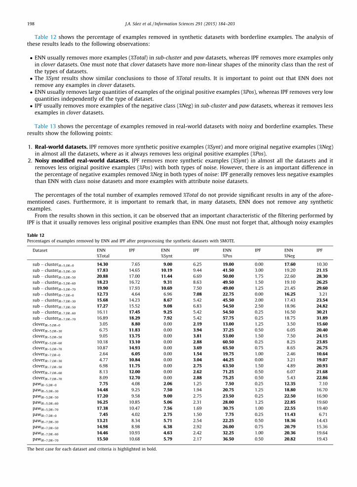
Table 12 shows the percentage of examples removed in synthetic datasets with borderline examples. The analysis ofthese results leads to the following observations:

� ENN usually removes more examples (%Total) in sub-cluster and paw datasets, whereas IPF removes more examples onlyin clover datasets. One must note that clover datasets have more non-linear shapes of the minority class than the rest ofthe types of datasets.� The %Synt results show similar conclusions to those of %Total results. It is important to point out that ENN does not

remove any examples in clover datasets.� ENN usually removes large quantities of examples of the original positive examples (%Pos), whereas IPF removes very low

quantities independently of the type of dataset.� IPF usually removes more examples of the negative class (%Neg) in sub-cluster and paw datasets, whereas it removes less

examples in clover datasets.

Table 13 shows the percentage of examples removed in real-world datasets with noisy and borderline examples. Theseresults show the following points:

1. Real-world datasets. IPF removes more synthetic positive examples (%Synt) and more original negative examples (%Neg)in almost all the datasets, where as it always removes less original positive examples (%Pos).

2. Noisy modified real-world datasets. IPF removes more synthetic examples (%Synt) in almost all the datasets and itremoves less original positive examples (%Pos) with both types of noise. However, there is an important difference inthe percentage of negative examples removed %Neg in both types of noise: IPF generally removes less negative examplesthan ENN with class noise datasets and more examples with attribute noise datasets.

The percentages of the total number of examples removed %Total do not provide significant results in any of the afore-mentioned cases. Furthermore, it is important to remark that, in many datasets, ENN does not remove any syntheticexamples.

From the results shown in this section, it can be observed that an important characteristic of the filtering performed byIPF is that it usually removes less original positive examples than ENN. One must not forget that, although noisy examples

Table 12Percentages of examples removed by ENN and IPF after preprocessing the synthetic datasets with SMOTE.

Dataset ENN IPF ENN IPF ENN IPF ENN IPF%Total %Synt %Pos %Neg

sub� clusterIR¼5;DR¼0 14.30 7.65 9.00 6.25 19.00 0.00 17.60 10.30sub� clusterIR¼5;DR¼30 17.83 14.65 10.19 9.44 41.50 3.00 19.20 21.15sub� clusterIR¼5;DR¼50 20.88 17.00 11.44 6.69 50.00 1.75 22.60 28.30sub� clusterIR¼5;DR¼60 18.23 16.72 9.31 8.63 49.50 1.50 19.10 26.25sub� clusterIR¼5;DR¼70 19.90 17.93 10.69 7.50 49.00 1.25 21.45 29.60sub� clusterIR¼7;DR¼0 12.73 4.64 6.96 7.08 22.75 0.00 16.25 3.21sub� clusterIR¼7;DR¼30 15.68 14.23 8.67 5.42 45.50 2.00 17.43 23.54sub� clusterIR¼7;DR¼50 17.27 15.52 9.08 6.83 54.50 2.50 18.96 24.82sub� clusterIR¼7;DR¼60 16.11 17.45 9.25 5.42 54.50 0.25 16.50 30.21sub� clusterIR¼7;DR¼70 16.89 18.29 7.92 5.42 57.75 0.25 18.75 31.89cloverIR¼5;DR¼0 3.05 8.80 0.00 2.19 13.00 1.25 3.50 15.60cloverIR¼5;DR¼30 6.75 11.83 0.00 3.94 37.25 0.50 6.05 20.40cloverIR¼5;DR¼50 9.05 13.75 0.00 3.81 53.00 1.50 7.50 24.15cloverIR¼5;DR¼60 10.18 13.10 0.00 2.88 60.50 0.25 8.25 23.85cloverIR¼5;DR¼70 10.87 14.93 0.00 3.69 65.50 0.75 8.65 26.75cloverIR¼7;DR¼0 2.64 6.05 0.00 1.54 19.75 1.00 2.46 10.64cloverIR¼7;DR¼30 4.77 10.84 0.00 3.04 44.25 0.00 3.21 19.07cloverIR¼7;DR¼50 6.98 11.75 0.00 2.75 63.50 1.50 4.89 20.93cloverIR¼7;DR¼60 8.13 12.00 0.00 2.62 71.25 0.50 6.07 21.68cloverIR¼7;DR¼70 8.09 12.70 0.00 2.88 75.25 0.50 5.43 22.86pawIR¼5;DR¼0 7.75 4.08 2.06 1.25 7.50 0.25 12.35 7.10pawIR¼5;DR¼30 14.48 9.25 7.50 1.94 20.75 1.25 18.80 16.70pawIR¼5;DR¼50 17.20 9.58 9.00 2.75 23.50 0.25 22.50 16.90pawIR¼5;DR¼60 16.25 10.85 5.06 2.31 28.00 1.25 22.85 19.60pawIR¼5;DR¼70 17.38 10.47 7.56 1.69 30.75 1.00 22.55 19.40pawIR¼7;DR¼0 7.45 4.02 2.75 1.50 7.75 0.25 11.43 6.71pawIR¼7;DR¼30 13.21 8.34 5.71 2.54 22.25 0.50 18.36 14.43pawIR¼7;DR¼50 14.98 8.98 6.38 2.92 26.00 0.75 20.79 15.36pawIR¼7;DR¼60 14.46 10.93 4.63 2.42 32.25 1.00 20.36 19.64pawIR¼7;DR¼70 15.50 10.68 5.79 2.17 36.50 0.50 20.82 19.43

The best case for each dataset and criteria is highlighted in bold.

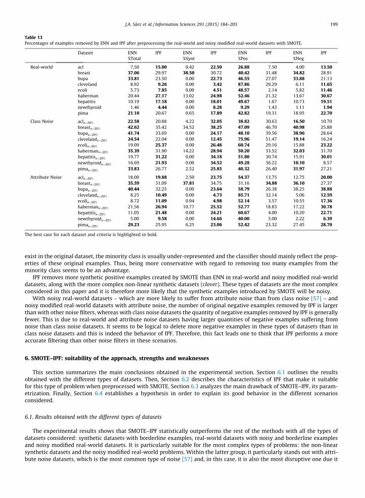
Table 13Percentages of examples removed by ENN and IPF after preprocessing the real-world and noisy modified real-world datasets with SMOTE.

Dataset ENN IPF ENN IPF ENN IPF ENN IPF%Total %Synt %Pos %Neg

Real-world acl 7.50 15.00 0.42 22.50 26.88 7.50 4.00 13.50breast 37.06 29.97 38.50 30.72 40.42 31.48 34.82 28.91bupa 33.81 23.50 0.00 22.73 46.55 27.07 33.88 21.13cleveland 8.92 9.26 0.00 3.42 87.86 29.29 6.11 11.65ecoli 5.73 7.85 0.00 4.51 48.57 2.14 5.82 11.46haberman 20.44 27.17 13.02 24.98 52.46 21.32 13.67 30.67hepatitis 10.19 17.18 0.00 18.01 49.67 1.67 10.73 19.51newthyroid 1.46 4.44 0.00 8.28 9.29 1.43 1.11 1.94pima 21.10 20.67 0.65 17.89 42.82 19.31 18.95 22.70

Class Noise aclx¼20% 22.58 20.88 4.22 32.05 38.82 30.63 16.50 10.70breastx¼20% 42.62 35.42 34.52 38.25 47.09 46.70 40.98 25.88bupax¼20% 41.74 33.69 0.00 24.17 48.10 39.56 38.96 28.64clevelandx¼20% 24.54 22.04 0.00 12.45 75.96 51.47 19.14 16.24ecolix¼20% 19.09 25.37 0.00 26.48 60.74 29.16 15.88 23.22habermanx¼20% 35.39 31.90 14.22 28.94 50.20 33.52 32.03 31.70hepatitisx¼20% 19.77 31.22 0.00 34.18 51.80 30.74 15.91 30.01newthyroidx¼20% 16.69 21.93 0.00 34.52 49.28 36.22 10.10 8.57pimax¼20% 33.83 26.77 2.52 25.85 40.32 26.40 31.97 27.21

Attribute Noise aclx¼20% 18.00 19.88 2.50 23.75 54.37 13.75 12.75 20.00breastx¼20% 35.59 31.09 37.81 34.75 31.16 34.88 36.10 27.37bupax¼20% 40.44 32.25 0.00 23.64 58.79 26.38 38.25 38.88clevelandx¼20% 8.25 10.49 0.00 4.73 85.71 32.14 5.06 12.59ecolix¼20% 8.72 11.09 0.94 4.98 52.14 3.57 10.55 17.36habermanx¼20% 21.56 26.94 10.77 25.52 52.77 18.83 17.22 30.78hepatitisx¼20% 11.05 21.48 0.00 24.21 60.67 4.00 10.20 22.71newthyroidx¼20% 5.00 9.58 0.00 14.66 40.00 5.00 2.22 6.39pimax¼20% 29.23 25.95 6.25 23.06 52.42 23.32 27.45 28.70

The best case for each dataset and criteria is highlighted in bold.


exist in the original dataset, the minority class is usually under-represented and the classifier should mainly reflect the prop-erties of these original examples. Thus, being more conservative with regard to removing too many examples from theminority class seems to be an advantage.

IPF removes more synthetic positive examples created by SMOTE than ENN in real-world and noisy modified real-worlddatasets, along with the more complex non-linear synthetic datasets (clover). These types of datasets are the most complexconsidered in this paper and it is therefore more likely that the synthetic examples introduced by SMOTE will be noisy.

With noisy real-world datasets – which are more likely to suffer from attribute noise than from class noise [57] – andnoisy modified real-world datasets with attribute noise, the number of original negative examples removed by IPF is largerthan with other noise filters, whereas with class noise datasets the quantity of negative examples removed by IPF is generallyfewer. This is due to real-world and attribute noise datasets having larger quantities of negative examples suffering fromnoise than class noise datasets. It seems to be logical to delete more negative examples in these types of datasets than inclass noise datasets and this is indeed the behavior of IPF. Therefore, this fact leads one to think that IPF performs a moreaccurate filtering than other noise filters in these scenarios.

6. SMOTE–IPF: suitability of the approach, strengths and weaknesses

This section summarizes the main conclusions obtained in the experimental section. Section 6.1 outlines the resultsobtained with the different types of datasets. Then, Section 6.2 describes the characteristics of IPF that make it suitablefor this type of problem when preprocessed with SMOTE. Section 6.3 analyzes the main drawback of SMOTE–IPF, its param-etrization. Finally, Section 6.4 establishes a hypothesis in order to explain its good behavior in the different scenariosconsidered.

6.1. Results obtained with the different types of datasets

The experimental results shows that SMOTE–IPF statistically outperforms the rest of the methods with all the types ofdatasets considered: synthetic datasets with borderline examples, real-world datasets with noisy and borderline examplesand noisy modified real-world datasets. It is particularly suitable for the most complex types of problems: the non-linearsynthetic datasets and the noisy modified real-world problems. Within the latter group, it particularly stands out with attri-bute noise datasets, which is the most common type of noise [57] and, in this case, it is also the most disruptive one due it


affecting both classes, whereas class noise only affects the majority class. The increase in the noise level makes the differ-ences in favor of SMOTE–IPF still more remarkable.

6.2. Characteristics of IPF and suitability for problems preprocessed with SMOTE

One important fact that makes IPF suitable for imbalanced datasets with noisy and borderline examples preprocessedwith SMOTE is its iterative elimination of noisy examples. This fact implies that the examples removed in one iteration donot influence detection in subsequent ones, resulting in a more accurate noise filtering.

Furthermore, the ensemble nature of IPF enables it to collect predictions from different classifiers which may provide abetter estimation of difficult noisy examples, as apposed to collecting information from a single classifier only [7]. IPF alsoenables the creation of more different classifiers – using random partitions, for example – than other ensemble-based filtersdue to it providing more freedom when creating the partitions from which these classifiers are built. Creating diversityamong the classifiers built is a key factor when ensembles of classifiers are used [34]. Finally, unlike other ensemble-basedfilters such as EF, which uses different classification algorithms to build the classifiers, IPF only requires one classificationalgorithm and is thus simpler.

6.3. On the parametrization of IPF

The choice of the different parameters of IPF can be seen as its main drawback, since there are numerous parameters andthe behavior of the filter is quite dependent on their values. From our many experiments we can draw several conclusionsregarding the influence of the different parameters on the performance results.

We have confirmed that using the majority scheme leads to better results than the consensus scheme since the number ofnoisy and borderline examples is large enough in comparison with the quantity of safe examples. The consensus scheme isvery strict in removing examples and does not enable one to remove enough examples to change the performancesignificantly.

Regarding the number of partitions, a larger number usually implies better noise detection (and also a higher preprocess-ing time) since the voting scheme depends on more information. It is recommended that this number be odd, in order toavoid ties in the votes of the classifiers. Considering n ¼ 9 partitions leads to a good balance between computational costand performance.

The way to build the partitions enables one to control the diversity among classifiers. We have tested different strategiesto create the partitions, such as stratified cross-validation – e.g. EF or CVCF – or random partitions. Random partitions wereconsidered because they lead to better performance results since, as was expected, the partitions and, therefore theclassifiers built, are more different.

The rest of the parameters allow a wider range of possibilities obtaining similar performances. Standard parametersrecommended by the authors of IPF also work well with our SMOTE-preprocessed imbalanced datasets, so they are fixedto k ¼ 3 iterations for the stop criterion and p ¼ 1% for the percentage of removed examples.

6.4. Hypothesis to explain the good behavior of IPF with respect to other filters

The properties of IPF seem to be well adapted to the removal of noisy and borderline examples, implying an advantageover other noise filters. Most of the noise filters combined with SMOTE, such as ENN or TL, have a noise identification basedon distances among examples to their nearest neighbors, taking into account their classes. This issue, although overlooked inthe literature, may be an important drawback: since SMOTE is based on the distance to the nearest neighbors to create a newpositive example, such synthetic examples introduced by SMOTE, although noisy, are highly likely to not be identified byfilters based on distances to the nearest neighbors. Using a noise identification method based on more complex rules, suchas IPF, enables one to group larger quantities of examples with similar characteristics, although exceptions exist that will beconsidered to be noise, avoiding the aforementioned problem and detecting noisy examples easily.

7. Concluding remarks

This paper has focused on the presence of noisy and borderline examples, which is an important and contemporaryresearch issue for learning classifiers from imbalanced data. It has been proposed to extend SMOTE with a new element,the IPF noise filter, to control the noise introduced by the balancing between classes produced by SMOTE and to makethe class boundaries more regular. The suitability of the approach in this scenario has been analyzed.

Synthetic imbalanced datasets with different shapes of the minority class, imbalance ratios and levels of borderline exam-ples have been considered. A set of real-world imbalanced datasets with different quantities of noisy and borderline exam-ples and other factors have been also considered. Additional noise has been introduced into the latter considering two noiseschemes: a class noise scheme and an attribute noise scheme. All these datasets have been preprocessed with our proposaland several re-sampling techniques that can be found in the literature. Finally, the C4.5 algorithm has been tested over thesepreprocessed datasets.


The values of the AUC measure have shown that our proposal has a notably better performance when dealing with imbal-anced datasets with noisy and borderline examples with both synthetic and real-world datasets. SMOTE–IPF also outper-forms the rest of the methods with the real-world datasets with additional noise. Our proposal especially outperformsthe rest of the methods with the more complex to learn datasets in each group of datasets: the non-linear synthetic datasetsand the attribute noise real-world datasets. These observations are supported by statistical tests.

The experiments performed with others classifiers (k-NN, SVM, RIPPER and PART) have provided similar results and con-clusions on the superiority of SMOTE–IPF to those shown for C4.5. Although statistical differences are less significant usingSVM and RIPPER with attribute noise datasets, SMOTE–IPF obtains the better performances and the aligned Friedman’sranks. The especially good results of SMOTE–IPF on the synthetic datasets using RIPPER and on the class noise datasets usingk-NN must also be pointed out. These results have been better than those of C4.5 shown here.

One must consider that the ensemble-nature of IPF, which constitutes a robust and accurate way of detecting mislabeledexamples, the iterative noise detection and elimination processes carried out and the possibility of controlling the diversitybetween classifiers are the key points of IPF which finally produce a more accurate filtering process. All these factors helpSMOTE–IPF to obtain better performances than other re-sampling techniques in the scenarios considered.

Acknowledgment

Supported by the National Project TIN2011-28488, and also by the Regional Projects P10-TIC-06858 and P11-TIC-9704.José A. Sáez holds an FPU scholarship from the Spanish Ministry of Education and Science. This paper is also supported by thePolish National Science Center under Grant No. DEC-2013/11/B/ST6/00963.

References

[1] J. Alcalá-Fdez, A. Fernández, J. Luengo, J. Derrac, S. García, L. Sánchez, F. Herrera, KEEL data-mining software tool: data set repository, integration ofalgorithms and experimental analysis framework, J. Multiple-Valued Logic Soft Comput. 17 (2011) 255–287.

[2] J. Alcalá-Fdez, L. Sánchez, S. García, M. del Jesus, S. Ventura, J. Garrell, J. Otero, C. Romero, J. Bacardit, V. Rivas, J. Fernández, F. Herrera, KEEL: a softwaretool to assess evolutionary algorithms for data mining problems, Soft Comput. – Fus. Found. Methodol. Appl. 13 (2009) 307–318.

[3] R. Barandela, J.S. Sánchez, V. García, E. Rangel, Strategies for learning in class imbalance problems, Pattern Recogn. 36 (2003) 849–851.[4] G. Batista, R. Prati, M. Monard, A study of the behavior of several methods for balancing machine learning training data, ACM SIGKDD Explor. Newslett.

6 (2004) 20–29.[5] U. Bhowan, M. Johnston, M. Zhang, Developing new fitness functions in genetic programming for classification with unbalanced data, IEEE Trans. Syst.

Man Cybern., Part B: Cybern. 42 (2012) 406–421.[6] A.P. Bradley, The use of the area under the ROC curve in the evaluation of machine learning algorithms, Pattern Recogn. 30 (1997) 1145–1159.[7] C.E. Brodley, M.A. Friedl, Identifying mislabeled training data, J. Artif. Intell. Res. 11 (1999) 131–167.[8] C. Bunkhumpornpat, K. Sinapiromsaran, C. Lursinsap, Safe-level-SMOTE: safe-level-synthetic minority over-sampling technique for handling the class

imbalanced problem, in: Proceedings of the 13th Pacific-Asia Conference on Advances in Knowledge Discovery and Data Mining, PAKDD ’09, Springer-Verlag, Berlin, Heidelberg, 2009, pp. 475–482.

[9] N.V. Chawla, K.W. Bowyer, L.O. Hall, W.P. Kegelmeyer, SMOTE: synthetic minority over-sampling technique, J. Artif. Intell. Res. 16 (2002) 321–357.[10] N.V. Chawla, D.A. Cieslak, L.O. Hall, A. Joshi, Automatically countering imbalance and its empirical relationship to cost, Data Min. Knowl. Discov. 17

(2008) 225–252.[11] N.V. Chawla, N. Japkowicz, A. Kotcz, Editorial: special issue on learning from imbalanced data sets, SIGKDD Explor. 6 (2004) 1–6.[12] W.W. Cohen, Fast effective rule induction, in: Proceedings of the Twelfth International Conference on Machine Learning, Morgan Kaufmann Publishers,

1995, pp. 115–123.[13] C. Cortes, V. Vapnik, Support vector networks, Mach. Learn. 20 (1995) 273–297.[14] J. Demšar, Statistical comparisons of classifiers over multiple data sets, J. Mach. Learn. Res. 7 (2006) 1–30.[15] A. Fernández, M.J. del Jesus, F. Herrera, On the 2-tuples based genetic tuning performance for fuzzy rule based classification systems in imbalanced

data-sets, Inf. Sci. 180 (2010) 1268–1291.[16] E. Frank, I.H. Witten, Generating accurate rule sets without global optimization, in: ICML98: Proceedings of the Fifteenth International Conference on

Machine Learning, Morgan Kaufmann Publishers Inc., San Francisco, CA, USA, 1998, pp. 144–151.[17] D. Gamberger, R. Boskovic, N. Lavrac, C. Groselj, Experiments with noise filtering in a medical domain, in: Proceedings of the Sixteenth International

Conference on Machine Learning, Morgan Kaufmann Publishers, 1999, pp. 143–151.[18] D. Gamberger, N. Lavrac, S. Dzeroski, Noise detection and elimination in data preprocessing: experiments in medical domains, Appl. Artif. Intell. 14

(2000) 205–223.[19] S. García, A. Fernández, J. Luengo, F. Herrera, Advanced nonparametric tests for multiple comparisons in the design of experiments in computational

intelligence and data mining: experimental analysis of power, Inf. Sci. 180 (2010) 2044–2064.[20] V. García, R. Alejo, J. Sánchez, J. Sotoca, R. Mollineda, Combined effects of class imbalance and class overlap on instance-based classification, in: E.

Corchado, H. Yin, V. Botti, C. Fyfe (Eds.), Intelligent Data Engineering and Automated Learning IDEAL 2006, Lecture Notes in Computer Science, vol.4224, Springer, Berlin/Heidelberg, 2006, pp. 371–378.

[21] V. García, R. Mollineda, J. Sánchez, On the k-NN performance in a challenging scenario of imbalance and overlapping, Pattern Anal. Appl. 11 (2008)269–280.

[22] V. García, J. Sánchez, R. Mollineda, An empirical study of the behavior of classifiers on imbalanced and overlapped data sets, in: L. Rueda, D. Mery, J.Kittler (Eds.), CIARP 2007, LNCS, vol. 4756, Springer, Heidelberg, 2007, pp. 397–406.

[23] H. Han, W.Y. Wang, B.H. Mao, Borderline-SMOTE: a new over-sampling method in imbalanced data sets learning, in: Proceedings of the 2005International Conference on Advances in Intelligent Computing – Volume Part I, Springer-Verlag, Berlin, Heidelberg, 2005, pp. 878–887.

[24] H. He, E. Garcia, Learning from imbalanced data, IEEE Trans. Data Knowl. Eng. 21 (2009) 1263–1284.[25] Y. Hochberg, A sharper Bonferroni procedure for multiple tests of significance, Biometrika 75 (1988) 800–803.[26] J. Hodges, E. Lehmann, Ranks methods for combination of independent experiments in analysis of variance, Ann. Math. Stat. 33 (1962) 482–497.[27] K. Huang, H. Yang, I. King, M.R. Lyu, Imbalanced learning with a biased minimax probability machine, IEEE Trans. Syst. Man Cybern., Part B: Cybern. 36

(2006) 913–923.[28] N. Japkowicz, Class imbalance: are we focusing on the right issue?, in: II Workshop on Learning from Imbalanced Data Sets, ICML, Morgan Kaufmann

Publishers Inc, 2003, pp. 17–23.[29] T. Jo, N. Japkowicz, Class Imbalances versus small disjuncts, SIGKDD Explor. 6 (2004) 40–49.

http://refhub.elsevier.com/S0020-0255(14)00856-1/h0005

































































[30] K.L. Kermanidis, The effect of borderline examples on language learning, J. Exp. Theor. Artif. Intell. 21 (2009) 19–42.[31] K.C. Khor, C.Y. Ting, S. Phon-Amnuaisuk, A cascaded classifier approach for improving detection rates on rare attack categories in network intrusion

detection, Appl. Intell. 36 (2012) 320–329.[32] T.M. Khoshgoftaar, P. Rebours, Improving software quality prediction by noise filtering techniques, J. Comput. Sci. Technol. 22 (2007) 387–396.[33] M. Kubat, S. Matwin, Addressing the curse of imbalanced training sets: one-sided selection, in: Proceedings of the 14th International Conference on

Machine Learning, Morgan Kaufmann, 1997, pp. 179–186.[34] L.I. Kuncheva, Diversity in multiple classifier systems, Inf. Fus. 6 (2005) 3–4.[35] V. López, A. Fernández, F. Herrera, On the importance of the validation technique for classification with imbalanced datasets: addressing covariate shift

when data is skewed, Inf. Sci. 257 (2014) 1–13.[36] V. López, I. Triguero, C.J. Carmona, S. García, F. Herrera, Addressing imbalanced classification with instance generation techniques: IPADE-ID,

Neurocomputing 126 (2014) 15–28.[37] T. Maciejewski, J. Stefanowski, Local neighbourhood extension of SMOTE for mining imbalanced data, in: Proceedings of IEEE Symposium on

Computational Intelligence and Data Mining, SSCI IEEE, IEEE Press, 2011, pp. 104–111.[38] R. Mathiasi Horta, B. Pires De Lima, C. Borges, A semi-deterministic ensemble strategy for imbalanced datasets (SDEID) applied to bankruptcy

prediction, WIT Trans. Inf. Commun. Technol. 40 (2008) 205–213.[39] G.J. McLachlan, Discriminant Analysis and Statistical Pattern Recognition, John Wiley and Sons, 2004.[40] K. Napierala, J. Stefanowski, S. Wilk, Learning from imbalanced data in presence of noisy and borderline examples, in: Rough Sets and Current Trends in

Computing, Lecture Notes in Computer Science, vol. 6086, Springer, Berlin/Heidelberg, 2010, pp. 158–167.[41] J.R. Quinlan, C4.5: Programs for Machine Learning, Morgan Kaufmann Publishers, San Francisco, CA, USA, 1993.[42] J.A. Sáez, M. Galar, J. Luengo, F. Herrera, Tackling the problem of classification with noisy data using multiple classifier systems: analysis of the

performance and robustness, Inf. Sci. 247 (2013) 1–20.[43] J.A. Sáez, M. Galar, J. Luengo, F. Herrera, Analyzing the presence of noise in multi-class problems: alleviating its influence with the one-vs-one

decomposition, Knowl. Inf. Syst. 38 (2014) 179–206.[44] J.A. Sáez, J. Luengo, F. Herrera, Predicting noise filtering efficacy with data complexity measures for nearest neighbor classification, Pattern Recogn. 46

(2013) 355–364.[45] K. Slowinski, J. Stefanowski, D. Siwinski, Application of rule induction and rough sets to verification of magnetic resonance diagnosis, Fund. Inform. 53

(2002) 345–363.[46] J. Stefanowski, Overlapping, rare examples and class decomposition in learning classifiers from imbalanced data, in: S. Ramanna, L.C. Jain, R.J. Howlett

(Eds.), Emerging Paradigms in Machine Learning, Smart Innovation, Systems and Technologies, vol. 13, Springer, Berlin, Heidelberg, 2013, pp. 277–306.[47] J. Stefanowski, S. Wilk, Selective pre-processing of imbalanced data for improving classification performance, in: I.Y. Song, J. Eder, T. Nguyen (Eds.),

Data Warehousing and Knowledge Discovery, Lecture Notes in Computer Science, vol. 5182, Springer, Berlin/Heidelberg, 2008, pp. 283–292.[48] C.T. Su, Y.H. Hsiao, An evaluation of the robustness of MTS for imbalanced data, IEEE Trans. Knowl. Data Eng. 19 (2007) 1321–1332.[49] A. Sun, E.P. Lim, Y. Liu, On strategies for imbalanced text classification using SVM: a comparative study, Decis. Support Syst. 48 (2009) 191–201.[50] Y. Sun, M.S. Kamel, A.K. Wong, Y. Wang, Cost-sensitive boosting for classification of imbalanced data, Pattern Recogn. 40 (2007) 3358–3378.[51] Y. Tang, Y. Zhang, N.V. Chawla, SVMs modeling for highly imbalanced classification, IEEE Trans. Syst. Man Cybern., Part B: Cybern. 39 (2009) 281–288.[52] F.B. Tek, A.G. Dempster, I. Kale, Parasite detection and identification for automated thin blood film malaria diagnosis, Comput. Vis. Image Understand.

114 (2010) 21–32.[53] I. Tomek, Two modifications of CNN, IEEE Trans. Syst. Man Commun. 6 (1976) 769–772.[54] S. Verbaeten, A.V. Assche, Ensemble methods for noise elimination in classification problems, in: Fourth International Workshop on Multiple Classifier

Systems, Springer, 2003, pp. 317–325.[55] D.L. Wilson, Asymptotic properties of nearest neighbor rules using edited data, IEEE Trans. Syst. Man Cybern. 2 (1972) 408–421.[56] D.R. Wilson, T.R. Martinez, Improved heterogeneous distance functions, J. Artif. Intell. Res. 6 (1997) 1–34.[57] X. Zhu, X. Wu, Class noise vs. attribute noise: a quantitative study, Artif. Intell. Rev. 22 (2004) 177–210.

José A. Sáez received his M.Sc. in Computer Science from the University of Granada (Granada, Spain) in 2009. He is currently aPh.D. student in the Department of Computer Science and Artificial Intelligence in the University of Granada. His main researchinterests include noisy data in classification, discretization methods and imbalanced learning.

Julián Luengo received the M.S. degree in computer science and the Ph.D. degree from the University of Granada, Granada,Spain, in 2006 and 2011 respectively. His research interests include machine learning and data mining, data preparation inknowledge discovery and data mining, missing values, data complexity and fuzzy systems.



























































Jerzy Stefanowski received the Ph.D. and Habilitation degrees in computer science from Poznan University of Technology,Poland, in 1994 and 2001, respectively. He is currently an Associate Professor in Institute of Computing Science, PoznanUniversity of Technology (specialization in Machine Learning and Knowledge Discovery from Data). His research interestsinclude: machine learning, data mining and intelligent decision support – in particular rule induction, multiple classifiers, datapre-processing; document clustering, mining sequence patterns and handling uncertainty in data. His work has also led toapplications in medicine, technical diagnostics and finance. He served as a reviewer for many international journals andconferences. His publication list covers over 120 journal and conference papers.

Francisco Herrera received his M.Sc. in Mathematics in 1988 and Ph.D. in Mathematics in 1991, both from the University ofGranada, Spain.He is currently a Professor in the Department of Computer Science and Artificial Intelligence at the University of Granada. He hasbeen the supervisor of 30 Ph.D. students. He has published more than 260 papers in international journals. He is coauthor of thebook ‘‘Genetic Fuzzy Systems: Evolutionary Tuning and Learning of Fuzzy Knowledge Bases’’ (World Scientific, 2001).He currently acts as Editor in Chief of the international journals ‘‘Information Fusion’’ (Elsevier) and ‘‘Progress in ArtificialIntelligence (Springer). He acts as an area editor of the International Journal of Computational Intelligence Systems and asso-ciated editor of the journals: IEEE Transactions on Fuzzy Systems, Information Sciences, Knowledge and Information Systems,Advances in Fuzzy Systems, and International Journal of Applied Metaheuristics Computing; and he serves as a member ofseveral journal editorial boards, among others: Fuzzy Sets and Systems, Applied Intelligence, Information Fusion, Knowledge-Based Systems, Evolutionary Intelligence, International Journal of Hybrid Intelligent Systems, Memetic Computation, and Swarmand Evolutionary Computation.

He received the following honors and awards: ECCAI Fellow 2009, IFSA Fellow 2013, 2010 Spanish National Award on Computer Science ARITMEL to the‘‘Spanish Engineer on Computer Science’’, International Cajastur ‘‘Mamdani’’ Prize for Soft Computing (Fourth Edition, 2010), IEEE Transactions on FuzzySystem Outstanding 2008 Paper Award (bestowed in 2011), 2011 Lotfi A. Zadeh Prize Best paper Award of the International Fuzzy Systems Association, and
2013 AEPIA Award to a scientific career in Artificial Intelligence (September 2013).His current research interests include computing with words and decision making, bibliometrics, data mining, data preparation, instance selection andgeneration, imperfect data, fuzzy rule based systems, genetic fuzzy systems, imbalanced classification, knowledge extraction based on evolutionaryalgorithms, memetic algorithms and genetic algorithms, biometrics, cloud computing and big data.

Documents

SMOTEâ€“IPF: Addressing the noisy and borderline examples