SMS Advanced Manual - International Centre for Theoretical ...indico.ictp.it/event/a09138/session/54/contribution/34/material/2/... · Creating and Editing Data ... How to export

SMS Advanced Manual

iii

Table Of ContentsIntroduction........................................................................................................................................................................ 1Introduction .................................................................................................................................................................... 1System Requirements to Run the Software .................................................................................................................... 5Things You Should Know to Run the Software ............................................................................................................... 5Getting Started............................................................................................................................................................... 7Registering SMS ............................................................................................................................................................ 8How to Use the Electronic Help...................................................................................................................................... 9

User Interface.................................................................................................................................................................. 11Menus .......................................................................................................................................................................... 11Main Windows.............................................................................................................................................................. 25

Data Processing .............................................................................................................................................................. 49Processing Data........................................................................................................................................................... 49

Data Management ........................................................................................................................................................... 51Data Management........................................................................................................................................................ 51Workspaces ................................................................................................................................................................. 51Projects........................................................................................................................................................................ 52

Mapping and Viewing Data .............................................................................................................................................. 53Mapping Data............................................................................................................................................................... 53Map Backgrounds ........................................................................................................................................................ 53Layering ....................................................................................................................................................................... 53Data Playback.............................................................................................................................................................. 543D Mapping and Plotting .............................................................................................................................................. 54

Legends........................................................................................................................................................................... 57Legends ....................................................................................................................................................................... 57

Creating and Editing Data................................................................................................................................................ 59Creating Data............................................................................................................................................................... 59Editing Data ................................................................................................................................................................. 62

Jobs and Tasks ............................................................................................................................................................... 65About Jobs and Tasks.................................................................................................................................................. 65Creating and Editing Jobs and Tasks ........................................................................................................................... 65Exporting Jobs and Tasks ............................................................................................................................................ 65

Data Analysis and Modification ........................................................................................................................................ 67Data Modification and Creation .................................................................................................................................... 67Analysis Wizard............................................................................................................................................................ 68Multi-Project Analysis ................................................................................................................................................... 70Spatial Data Finder ...................................................................................................................................................... 70Financial Tracking ........................................................................................................................................................ 70

Importing/Exporting Data and Setup Information.............................................................................................................. 73Importing Data.............................................................................................................................................................. 73Exporting Data ............................................................................................................................................................. 74Device Setup................................................................................................................................................................ 75

Printing (Reports, Charts, Map Layouts, etc).................................................................................................................... 77Printing......................................................................................................................................................................... 77

Data Backup, Transfer, and Maintenance ........................................................................................................................ 79Backing up and Restoring Data.................................................................................................................................... 79Transfer Settings, Setup Files, Etc. .............................................................................................................................. 79

SMS Advanced Manual

iv

Database Maintenance ................................................................................................................................................ 81How to ... ......................................................................................................................................................................... 83How to read logged data files into the system............................................................................................................... 83How to migrate your data from Precision Map 2000 or Instant Yield Map Software ...................................................... 83How to import Greenstar data....................................................................................................................................... 83How to reprocess data. ................................................................................................................................................ 84How to set your map projection. ................................................................................................................................... 84Using the Management Tree ........................................................................................................................................ 84Using the Preview Window........................................................................................................................................... 85Using the Calendar View. ............................................................................................................................................. 85How to make a map ..................................................................................................................................................... 86How to Add a Layer to a Map. ...................................................................................................................................... 86How to display the 3D Terrain View.............................................................................................................................. 87Using the Layer Window .............................................................................................................................................. 87How to adjust layer and attribute/property options. ....................................................................................................... 88How to edit point data................................................................................................................................................... 88How to straighten a pass on a point dataset. ................................................................................................................ 89How to edit a legend..................................................................................................................................................... 89How to freeze a boundary. ........................................................................................................................................... 89How to create a new attribute....................................................................................................................................... 89How to create a new property....................................................................................................................................... 90How to create/edit a custom Operation......................................................................................................................... 90How to define Products ................................................................................................................................................ 91How to add a property to a management item or dataset.............................................................................................. 91How to edit property data. ............................................................................................................................................ 92How to enter Financial Tracking entries........................................................................................................................ 92How to generate a Financial Tracking report. ............................................................................................................... 93How to create a 3D Plot. .............................................................................................................................................. 94How to create a boundary. ........................................................................................................................................... 94How to edit a boundary. ............................................................................................................................................... 95How to create a crop plan............................................................................................................................................. 95How to edit a crop plan................................................................................................................................................. 96How to create a generic dataset. .................................................................................................................................. 96How to use the Average Data by Polygon Tool............................................................................................................. 96How to use the Vector Overlay Tool. ............................................................................................................................ 97How to edit generic data............................................................................................................................................... 97How to create a guidance dataset. ............................................................................................................................... 97How to create navigation points.................................................................................................................................... 98How to edit navigation points........................................................................................................................................ 98How to create a variable rate prescription..................................................................................................................... 98How to edit a prescription dataset. ............................................................................................................................... 99How to create a soil sampling dataset. ....................................................................................................................... 100How to edit soil sampling data. ................................................................................................................................... 101How to add Buffer Regions to an object...................................................................................................................... 102How to edit an image.................................................................................................................................................. 102How to create spatial notes. ....................................................................................................................................... 102How to edit spatial notes. ........................................................................................................................................... 103How to create associated data. .................................................................................................................................. 103How to edit an associated dataset. ............................................................................................................................. 103

Table Of Contents

v

How to create split planter data. ................................................................................................................................. 104How to add a simple analysis function(s).................................................................................................................... 104How to edit a simple analysis function(s). ................................................................................................................... 106How to remove a simple analysis function(s). ............................................................................................................. 106How to merge cotton pickings..................................................................................................................................... 106How to straighten a pass on a point dataset. .............................................................................................................. 107How to update a merged cotton dataset. .................................................................................................................... 107How to generate correlation results. ........................................................................................................................... 107How to generate a cluster analysis dataset ................................................................................................................ 108How to generate comparison results. ......................................................................................................................... 109How to run a batch comparison analysis. ................................................................................................................... 110How to write an analysis equation .............................................................................................................................. 111How to generate a Multi-Year averages dataset. ........................................................................................................ 114How to generate a Profit/Loss dataset........................................................................................................................ 114How to generate an NDVI dataset. ............................................................................................................................. 115How to generate a terrain analysis dataset................................................................................................................. 116How to search for spatial data using the Spatial Data Finder. ..................................................................................... 116How to save a workspace........................................................................................................................................... 117How to open a workspace. ......................................................................................................................................... 117How to geo-reference an Image. ................................................................................................................................ 117How to set a map background(s)................................................................................................................................ 118How to manually move a Farm................................................................................................................................... 118How to create a Job and Task(s)................................................................................................................................ 118How to export a Job. .................................................................................................................................................. 119How to manually move a Field.................................................................................................................................... 119How to manually move other management items (Year, Load, etc.). .......................................................................... 120How to spatially sort Fields into Farms. ...................................................................................................................... 120How to spatially sort Loads/Regions into Fields.......................................................................................................... 120How to split and sort a load or region. ........................................................................................................................ 121How to query a single layer. ....................................................................................................................................... 121How to query multiple layers. ..................................................................................................................................... 121How to export a bitmap or other image file type.......................................................................................................... 122How to import a GeoTIFF image file. .......................................................................................................................... 122How to import an ESRI Shape, MapInfo Mid/Mif, DEM, or TIGER file......................................................................... 122How to batch import data (i.e. ESRI Shape,and text files)........................................................................................... 123How to export an ESRI Shape or MapInfo Mid/Mif file. ............................................................................................... 124How to import an ASCII text file.................................................................................................................................. 124How to import non-spatial data (i.e. Soil Lab Results)................................................................................................. 125How to export an ASCII text file.................................................................................................................................. 125How to import data using a template. ......................................................................................................................... 126How to export a TGT prescription file. ........................................................................................................................ 126How to export a Case IH or New Holland Voyager PRD Prescription file. ................................................................... 126How to export an Ag Leader Basic or Advanced format file. ....................................................................................... 127How to print a map of the current layer. ...................................................................................................................... 127How to print a map of all layers. ................................................................................................................................. 127How to print the current map. ..................................................................................................................................... 127How to print a custom map......................................................................................................................................... 128How to print the Summary Window Information. ......................................................................................................... 128How to print the Map Window summary information. .................................................................................................. 128

SMS Advanced Manual

vi

How to print the query results information................................................................................................................... 128How to print a report................................................................................................................................................... 128How to create a custom report.................................................................................................................................... 129How to print a chart. ................................................................................................................................................... 130How to create a custom chart. .................................................................................................................................... 130How to create a backup of your systems data. ........................................................................................................... 131How to restore a data backup file. .............................................................................................................................. 131How to export and import Transfer Information........................................................................................................... 131

Troubleshooting............................................................................................................................................................. 133Mapping Problems ..................................................................................................................................................... 133Printing Problems....................................................................................................................................................... 133Restore Problems ...................................................................................................................................................... 134Tutorial Problems ....................................................................................................................................................... 134

Reference Information ................................................................................................................................................... 135Glossary of Terminology ............................................................................................................................................ 135GPS Coordinate Conversions .................................................................................................................................... 136Ag Leader Basic and Advanced format ...................................................................................................................... 137Export Data Formats .................................................................................................................................................. 138SDTS to DEM Converter ............................................................................................................................................ 139

Index ............................................................................................................................................................................. 141

1

��

IntroductionAg Leader Technology is proud to offer SMS Advanced to you and thanks you for using our software. SMS stands forSpatial Management System. The word "Spatial" means involving or relating to space. That�s exactly what your Farmand Fields are. The space where you are involved (working) every day and the space that relates to all your businessdecisions.

SMS is the easiest to use, yet most powerful precision farming software package available for use with your Ag Leaderequipment. It provides unique features to support all the Ag Leader precision farming equipment that you currently ownand also helps integrate information that you may have from other sources or equipment. Simply put, you have chosena software package that will continue to grow and adapt with your Ag Leader equipment, current and future, which noother software package will be able to match.

SMS provides you with the following functionality:

�� Archiving of YLD, VYG, NH LOG, and GSY files.Imports all harvest log files created by Ag Leader, Case IH, JD Greenstar, and New Holland yield monitor systems.

�� Auto detection of new files.Can automatically search your PCMCIA card for new files that it has not read in before and automatically list themas files to be read in, while excluding the ones that it has already read in.

�� Import/export of Shape, ASCII text, GeoTIFF, and bitmap, JPEG, and TIFF image files.Provides you with a great deal of flexibility in terms of allowing the import of data from sources other than yourcurrent equipment. This includes ESRI Shape files, which are commonly used for transferring information betweensoftware packages. The GeoTIFF import allows you to bring images files into the system that are already spatiallyreferenced, which means you don�t have to geo-reference the image to bring it in. Imported data, except forimages, has summary information, can be charted, displayed in reports, queried, mapped, etc. The software alsoallows you to export data in these import formats so that you can provide information to outside sources that maynot be able to handle your monitors files directly. Exports can be customized and saved as export templates foreasier export and use outside of the software.

�� Batch processing of YLD files.Allows you to read multiple files from the same monitor into the management system using the settings that youmake for the first file. This automates the process of bringing in a large number of files and requires lesssupervision of the file reading process. This is an excellent tool for loading in files from previous years that youhave stored in another software program.

�� Processing of data to adjust, filter, or correct data.Ability to set such items as Flow delays, manual moisture, GPS filtering and correction, etc. before or after the datahas been entered into the software. This allows for greater flexibility in making sure that your data is displayedproperly.

�� Management of non-spatial and spatial data.Even if you are not using GPS with your equipment, you can still benefit from the softwares data managementcapabilities. Summary information and reports can still be viewed for data that was collected without GPS.

�� Entry of Manual Summary values.Provides the ability to enter in manual attribute values for a dataset, such as entering a manual area or adjustingthe total weight for a load. These manual values can be display along with the monitor or spatial summary valuesor by themselves.

�� Automated download of Terraserver images.Allows the automatic downloading and import of aerial images for each field in your system from the MicrosoftTerraserver over the internet.

�� Automatic Map Projection selection.This feature helps make sure that when you are viewing and working with your spatial data that it is displayed asaccurately as possible. Since the earth is not a perfect sphere, different locations on the earth will map improperlywithout regional corrections for the earth�s surface. This feature automatically selects a Datum and Projection thefirst time you try to make a map and a projection has not already been set that best matches the dataset that youare trying to map. This can manually be performed for each Grower in the Management Tree under the Projectiontab.

SMS Advanced Manual

2

�� Option to sort data by geography.This feature, the Spatial Sorter, provides a powerful tool for organizing and sorting your data, no matter how it wascollected or what model of monitor was used. You can set a boundary for a Field and/or a Farm and the softwarecan sort the Fields that you have loaded into the system into the Farm area that you have specified. The data thatyou have collected can also be sorted into a specific Field. This is very useful if you have data from multiple years,different monitors in the same fields, did not use the same names for fields every year, or used different fieldnumbers for the same field in different years. No matter what your situation is, the softwares Spatial Sorter willorganize your data that has GPS into the right geographic area that you have defined. All data, expect for images,that is read into the system can be sorted by the Spatial Sorter. The Spatial Sorter can also be run from theManagement Tree at the Grower, Farm, or Field levels to limit what data the sorter has to search through and thatwill potentially be moved. Spatial Sorting can also be performed when archiving files into the system.

�� Resource Tracking and Product DefinitionAllows you to define and assign Operators, Vehicles, Implements, and Product Containers to the data you log withyour monitor or field device or create in the software. Products can also be fully defined based on their intendedusage and properties. By assigning and defining these items you can add more detailed information to yourreports, charts, or maps and view new calculated attributes such as Fuel Used/Needed, Fuel Refills, ProductUsed/Needed, Product Refills, etc.

�� Creation of Split Planter data.Allows the creation of split planter data from As-Applied log data or Site Verification data. The software takes yourdata that was logged as a single product and rate by your monitor or field computer and splits the data into twonew datasets that have their own product and rates that can then be mapped to properly show where, what, andhow much you planted during your hybrid/variety trials.

�� Creation of device setup files.Allows the creation of setup configurations that can be used to export setup information for a monitor or other fielddevice, such as loading in Field Names from the desktop software.

�� Multi-layer data display and control.Provides you with the ability to display separate layers of data on a map at the same time and control the visibilityand order of them as well. This means that you can display an imported soil map on top of your yield map andapplication maps on the same screen and control the colors, map type, and transparency for each layer.

�� Layer transparency.Layer transparency allows you set a value that corresponds to how much you can see through a layer on thescreen. This is extremely useful when overlaying data for the same spatial area so that you can see featuresabove or below the layers that are displayed. It also provides feedback for "as applied" maps to show where youoverlapped and visually by how much.

�� Map and Layer Options.Provides a great deal of flexibility in the options that can be set for the display and interaction with data that ismapped. Tooltip, query, and label settings can be set for the display of information in the system. Sub-layersettings can be made for the display of Marks and Notes. And specific settings can be made that apply to amapped attribute or property. Settings for the attribute or property include display, drawing, and gridding options.

�� 3D Terrain View on Maps.Allows the viewing of your maps in 3D, based on the actual terrain of your fields. This option can be toggled on andoff from the Map Toolbar and is an integrated part of viewing your data. The terrain data comes automatically fromthe GPS that you log during field operations or from external files such as TOPO data logged by a high accuracyGPS receiver or a DEM (Digital Elevation Map).

�� 3D data plotting.Allows the generation of 3D plots from selected data. this option differs from the 3D Terrain View in that it allowsthe selection of any of the numerical based attributes in a dataset for plotting in 3D. This is a very useful tool forbetter visualizing your data.

�� Creation of variable rate prescriptions.Provides an easy to use wizard that helps you manually generate a variable rate prescription that can be exportedas a TGT prescription file for use in the PF3000 or PF3000 Pro or as an ESRI Shape or MID/MIF file for use inother devices. Prescriptions can also be created as a raster or vector type.

�� Analysis functions.SMS Advanced provide very powerful tools for analyzing the data that you collect or import. Analysis wizards, thatwalk you thorough the analysis process, are provided for Comparison Analysis, Equation Writing, Multi-YearAveraging, NDVI Analysis, Profit/Loss Analysis, and Slope Analysis. These tools can take those years worth ofdata you've been collecting and put them to work helping you improve your operation. Analysis functions can evenbe run in batch mode to help increase your productivity and automate your analysis.

Introduction

3

�� Ability to management your data by ProjectSMS Advanced allows you to create and manage Projects, which keep data from different growers, farms, etc inseparate databases and storage locations. This is very useful to help keep any single database and data directoryfrom getting to large, provides privacy and security for data from different people, and allows for the easy setup andtransfer of a customers data for them.

�� Ability to save a workspace.This feature allows you to save what you are currently working on, shutdown the program, restart the program, andopen the saved workspace and continue where you left off. For example if you had two maps open with threelayers in each that you had been working on, you could save a workspace, close the program, and come back in aweek and pull up the same maps and layers by just opening the saved workspace.

�� Creation of notes.Three different types of notes can be added to data, maps, or management items. Layer Notes can be added thatare tied to the dataset they are added to, such as a specific load. Landmark notes can be added that mark a fixedlocation on your farm that you wanted shown on any map that is made, such as a well or your home place. The lasttype of note is an associated note that ties to an management item(s) and is not mapped based. This allows you tomake notes that can be viewed and printed without mapping.

�� Ability to create and manage buffer zones.Buffer zones (polygons) can be created for point, line, or polygon objects in the system. The buffers are then linkedto whatever object you create them off of and will always be available for display, query, analysis when you areworking with that object. So if you can keep track and maintain a buffer zone you have to keep around certain fieldboundaries with out having to remember or find the buffer data for that field, its always right at your finger tips whenyou're working with the boundary for that field.

�� Financial TrackingFinancial Tracking allows you to enter in your expense and income values and tie them to your fields, operations,and products. The flexible entry system allows you to either provide little detail of expense and income values byentering in overall totals or per unit rates or you can be very detailed and itemize your expense and income values,its your decision. Once your entries have been made you can then generate profit/loss reports, perform spatialprofit/loss analysis per field, or display financial values per dataset layer in your summaries and maps.

�� Entry of Scale Ticket information.Allows the entry of scale ticket information for record keeping purposes. A standard entry form allows consistententry of scale tickets and allows you to view or print tickets. Scale tickets are what we called Associated data andare tied to a management item(s) and not to maps or layers.

�� Ability to print charts.Charts of your data can be created quickly and easily. You can print various types of charts including bar, pie, andline charts. Charts can be created that display information for your entire farm and all the years you have collecteddata or for a single field and year, it is up to you. In SMS Advanced you can also build your own custom charts.

�� Calendar ViewThis feature provides a unique way to select, view, and summarize your data. It uses time and events that happenduring time spans to display your data. You can for example see on the calendar that your Soybean harvest lastedfrom late September till late October and by clicking on that event listed on the calendar you can see a summary ofall the soybean harvest as well as map all the data collected for the soybean harvest with one click of your mousebutton.

�� Customizable summary display.Allows you to change the contents and ordering of information in the general and map summaries that aredisplayed when you select management items or have data mapped. You can even set the attributes to display indifferent units.

�� Selection and Drawing Tools.Provides a wide range of selection and drawing tools that allow you to create your own datasets, such as tile linesor polygon regions or make complex selections such as circular areas. You can even assign or create newattributes to go with these new objects that you are creating and also enter your own values for them.

�� Support for Soil Sampling plans and results.Provides specific support for creating soil sampling plans, managing this data, and allowing the manual entry of soiltest results or the importing of data from ASCII text (CSV, TXT) or DBF(dbase) files. Sample points can bemanually added or created through a sampling wizard that guides you through the process of creating griddedsample plans. Soil sample results data such a Soil pH or Soil OM can be mapped and contoured using inverseweighted distance or kriging interpolation methods.

�� Query Selection tool.

SMS Advanced Manual

4

This feature provides an extremely powerful tool for selecting exactly what data you want for queries, copying, orediting. The query selection tool allows you to define query filters that will select only the data in a dataset thatmeets your criteria. An example would be to create a set of filters that only select yield greater than 150 bu/ac andMoisture less than 17%.

�� Monitor Tree.Allows the viewing of your data collected with Case IH, Ag Leader, and New Holland monitors in two ways. Themain method is using the Main Management Tree, which manages data logically. The Monitor Tree adds adifferent dimension to the data management and displays only the data that was logged by an Case IH, NewHolland, or Ag Leader monitor and displays the management items as they were logged in the monitor. We call thisa physical tree, which means it is directly linked to what was logged. You can view and map data based on whichmonitor it can from and also see what field numbers data was logged to and the names that were used.

�� Grower, Farm, and Field summary report printing.Quick and easy selection of standard reports based on filters that you select. If you want to see a report for all theyears that a crop type such as corn was grown for a certain field you can set this in the report filter. You can alsoadd an image to the report title bar, such as a business logo. Reports can also be created as an HTML page foruse on the Internet. In SMS Advanced you can also build your own custom reports.

�� Custom map printouts.Provides a number of print options. One of the most powerful options is the ability to create custom map layouts.This feature allows you to decide what you would like to see on your map printouts and save the layout to be usedthe next time you need to create this type of printout. For example if you wanted to create a map that included aYield, elevation, and moisture map on the same page along with their legends you could lay this out and see whatit looked like before you printed. Charts of the data being mapped can also be added to the layout. You can alsosave layouts as image files such as BMP, JPEG, and TIFF (uncompressed) for use on presentations, the web, orediting and printing through an image viewer program.

�� Transfer of Settings and Setup files.Allows the transfer through one easy to use process and file of such things as backgrounds, custom legends,custom reports and charts, etc to another user of the software or to another project within your system. This is avery powerful tool for working with customers or multiple office locations where you might want share a customreport or chart that has been designed.

�� Batch Functions.A number of batch functions are provided that help automate various functions that normally can be very timeconsuming, but when run in batch can provide tremendous time saving and efficiency increases. Base functionsinclude Reprocess Data, Regenerate Boundary, Split Loads, etc. SMS Advanced goes a step further providesfunctions such as batch Import, Export, Print Layer, etc.

�� Automatic creation of field boundaries based on collected data.Automatically creates a boundary area for all log data that is read into the system. This auto boundary area isupdated when new data is read into the system that belongs to that field. It is also displayed in the PreviewWindow by default until actual load data is selected for that field from the Management Tree.

�� Export of Mark data.This export option allows you to export mark data that you have collected with your monitor system.

�� Program backup utility that creates a restorable backup of all the data in the system.With the amount of data that you are collecting and entering into the system a method to make sure that your dataand settings are properly backed-up is needed. The software provides a tool that creates a compressed copy of allthe data and settings that you have in the program that can be restored at any time. This compressed backup canbe stored on a removable media such as a CD-R, Zip drive, etc. If you get a new computer or something happensto your current machine that requires you to reformat or loose your data then after reinstalling the software you canrestore the backup and start working again from the point where you created the backup.

�� File Viewer function.Allows you to select a file that is archived in the system and see the contents of that file, such as which fields andloads have GPS and how many points there are. It also indicates if a load is not currently in the database andallows you to process the file so that its information is entered into the system properly.

�� Ag Leader Advanced and Basic export for grain harvest data.Ability to select grain harvest data and export it as Ag Leader Advanced or Basic files. This allows you flexibility insharing your data with other programs that have a standard import for yield data formatted this way.

�� Query tools, both single and multi-layer.Allows the user to query through a single layer, multiple layers, or use one layer as a "cookie cutter" to cut throughthe intersected area/objects below the selection area. Selection tools are also provided that allow the selection of

Introduction

5

individual points, rectangular regions, circles, ellipses, user drawn polygon regions, and filters. Query results arereported in a window below the map and can also be printed out.

�� Default legend settings for product/crops and associated attributes.Legends for a particular crop/product with an attribute such as yield can be set so that when that crop/product andattribute are selected the legend that you set will automatically appear. Legends can be set to only appear for acertain dataset, such as a field that may have contained test plots that you would like to use a special legend for.

�� And many other exciting features.There are a number of other exciting features that will help make your experience with the software moreenjoyable and productive. Please read through the rest of the help information or just explore through the programto discover what our software can do for you.

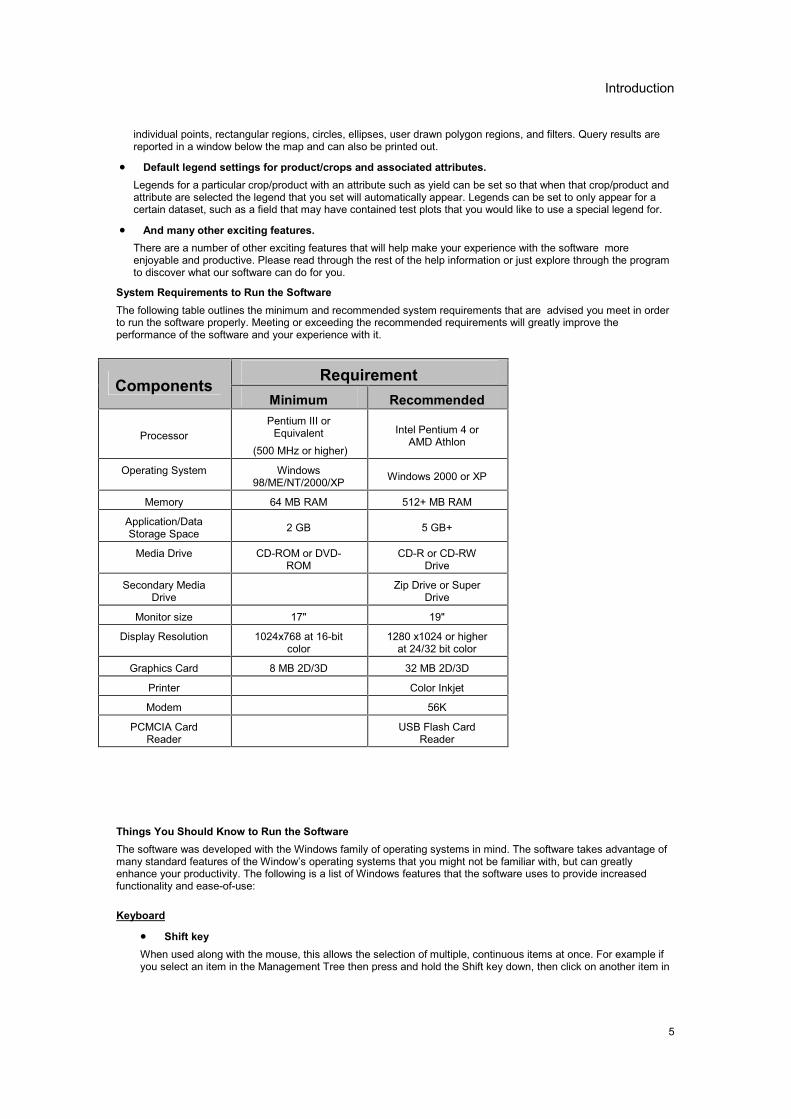
System Requirements to Run the SoftwareThe following table outlines the minimum and recommended system requirements that are advised you meet in orderto run the software properly. Meeting or exceeding the recommended requirements will greatly improve theperformance of the software and your experience with it.

RequirementComponentsMinimum Recommended

ProcessorPentium III orEquivalent

(500 MHz or higher)

Intel Pentium 4 orAMD Athlon

Operating System Windows98/ME/NT/2000/XP Windows 2000 or XP

Memory 64 MB RAM 512+ MB RAM

Application/DataStorage Space 2 GB 5 GB+

Media Drive CD-ROM or DVD-ROM

CD-R or CD-RWDrive

Secondary MediaDrive

Zip Drive or SuperDrive

Monitor size 17" 19"

Display Resolution 1024x768 at 16-bitcolor

1280 x1024 or higherat 24/32 bit color

Graphics Card 8 MB 2D/3D 32 MB 2D/3D

Printer Color Inkjet

Modem 56K

PCMCIA CardReader

USB Flash CardReader

Things You Should Know to Run the SoftwareThe software was developed with the Windows family of operating systems in mind. The software takes advantage ofmany standard features of the Window�s operating systems that you might not be familiar with, but can greatlyenhance your productivity. The following is a list of Windows features that the software uses to provide increasedfunctionality and ease-of-use:

Keyboard

�� Shift keyWhen used along with the mouse, this allows the selection of multiple, continuous items at once. For example ifyou select an item in the Management Tree then press and hold the Shift key down, then click on another item in

SMS Advanced Manual

6

the Management Tree, all the selections between your first and last selections will be highlighted and selected.Release the Shift key and the items will remain selected until the next selection with your mouse.

�� Ctrl KeyWhen used along with the mouse, this allows the selection of multiple non-consecutive items. For example if youwanted to select two fields from the Management Tree to map at the same time but there were 4 fields in the listbetween them, you would move your cursor over the first field, click the left mouse button to highlight and selectit. Then press and hold the Ctrl key and repeat the previous step to select the other field. Now release the Ctrlkey and both fields will remain selected until your next mouse click.

�� Arrow KeysAllow the user to move through selected lists instead of using the mouse to make each selection. This can beused to quickly move up and down in the Management Tree if a selection has already been made in the tree withthe mouse. It also allows the opening/closing of a branch in the tree. When a map is active in the software thearrow keys also serve as panning tools.

�� " + " and " � " Keys on Numeric KeypadUse these keys to zoom in and out on a map.

�� Home KeyPress this key to zoom and world and center the data in question.

�� F1 KeyPressing this key brings up the help for the current selection.

�� Other Keyboard ShortcutsFunction Key(s) to Press to Activate

Measure CTRL + MMulti-Line Measure CTRL + LCopy Selection CTRL + CPaste CTRL + VCut Selection CTRL + XUndo CTRL + ZRedo CTRL + YReset Cursor ENDDelete Selection DELETEMove Selection CTRL + EMerge Selections CTRL + RSnap to Start Point F2Snap to Center F3Snap to Midpoint F4Snap to Endpoint F5Snap to Closest F6Snap to Vertex F7Snap Off F8

Mouse

�� Clicking on an object or areaPoint the cursor to or over the desired object or area and press the left mouse buttononce and release.

�� Double clickingPoint the cursor to or over the desired object or area and quickly press and releasethe left mouse button twice.

�� Dragging ObjectsTo drag an object such as a window, move your cursor over the object, click and hold down the left mouse button,and then move the object to the desired location and release the left mouse button.

Introduction

7

�� The WheelIf you have a Windows operating system that supports a mouse with a wheel, such as the MS Intellimouse, thenyou can use the wheel for several functions, if your mouse has a wheel.

�� Scrolling � If a scroll bar is available in a window or dialog, move the cursor into that window ordialog and roll the wheel forward or back and the scroll bar should move accordingly.

�� Zoom � Holding the Ctrl key down and rolling the wheel forward or back zooms the current map inand out. This will even work on the Preview Window if the cursor is located over it.

�� Pan � Rolling the wheel forward or back, pans the current map up and down. Holding the Shift keydown and rolling the wheel forward and back will pan the current map left and right. This will alsowork on the Preview Window if the cursor is located over it.

Adjusting and Docking Windows

All the windows that comprise the software�s main window can be adjusted to a different size, and some can beundocked from there current location and moved around the screen as separate windows from the main window. Toadjust the size of a window move your cursor over the border of a window until you see a symbol with two parallel barsand arrows on each side. When this icon appears click and hold the left mouse button and drag the edge to adjust thesize of the window. This is most useful for adjusting the size of the Layer window to view more of the legend, or theopposite to see a larger map. To undock windows, and view them as separate floating windows, click on the graydouble bar above a window, click and hold the left mouse button down, and drag the window to a new location. Thewindow will now appear as a separate window from the main window. To re-dock the window with the main window,click and hold the left mouse button down in the area at the top of the window and drag the window until your cursorcrosses one of the edges of the main window. The window will then automatically dock.

Shortcut Menus

Shortcut menus appear when you move your cursor over an object and click the right mouse button. Shortcut menusprovided access to specific feature for an object or a quicker method of getting to common functions.

Getting Started

InstallationIf you haven�t already done so, install the software on your computer. It is recommended that you install it on a storagedrive other than your main boot drive that contains your operating system, which is normally your C:\ drive. This isespecially true if your C drive is partitioned and is less than 2GB in size. The reason for this recommendation is due tothe amount of data that must be stored and is generated by your precision farming activities. If you have a smaller Cdrive you could quickly fill the drive up or hinder performance of your computer by using to much of the boot drivesstorage and operation memory.Follow these steps to install the software on your computer from a CD:

1. Insert the software CD into your CD-ROM or DVD-ROM drive. The CD menu should now automatically start-up, if it does not, then click on the My Computer icon and open your CD-ROM or DVD-ROM drive by double-clicking on it.

2. Follow the directions on the screen to install the software.SMS Advanced Install OptionsSMS Advanced can either be installed as either a Single User install or a Networked User install.

�� Single User - Select this option if you will be installing the software on a single computer and aren'tintending to run it across a network with multiple users.

�� Networked Users - Select this option if you want all your data stored on a centralized server where itcan be accessed by multiple users. In this configuration if another user on the network has a projectopen you can not open it until they close it.

Migration from version 5.0X:If you have version 5.0X installed on your computer you have the option to migrate the data and settings from thatversion of the software to the new 5.5 version. Since internally there are number of differences between versions, themigration can be a lengthy process depending on the amount of data in your system and your computers capabilities.Follow these steps to migrate from 5.0X to v5.5:

1. Make sure that you have created a Backup in the software or have at least copied your DATA directory,which by default is located in the directory where you installed the software on. This will insure that your datais safe should something go wrong during the migration.

SMS Advanced Manual

8

2. Once you have your data backed up, insert the software CD into your CD-ROM or DVD-ROM drive. The CDmenu should now automatically start-up, if it does not, then click on the My Computer icon and open yourCD-ROM or DVD-ROM drive by double-clicking on it.

3. Click the Install button and follow the installation instructions.4. Once the install is complete, start software.5. You will now be prompted by a message about the migration process starting. Depending on your computer

and the amount of data you have this could take as much as two hours to complete or less than 15 minutes.Click OK to start the migration or Cancel if you would rather do the migration a different time. If you clickCancel you will not be able to run software until you complete the migration, which you will be prompted todo every time you try to start software until it migrates the data..

6. Once the migration completes, the software will start and all your information from v4.5 should have beenmigrated and accessible just like it was before the installation and migration to v5.0.

NOTE: V 1.XX, V2.X, v3.XX, v4.0X, and v4.5 migration is not supported by version 5.5. In addition,backups created in v1.XX, v2.XX, v3.XX, v4.0X, or v4.5 are also not supported. If you are still runningversion 1.XX, 2.XX, v3.XX, v4.0X,or v4.5 then you must first install a version of 2.0. 3.0, 4.0X, or 4.5, let itperform it�s migration, then install version 5.5 as described above and then let it perform the migrationfrom the previous versions to v5.5. Please contact Technical Support if you have any questions orconcerns about this process.

Initial SetupOnce the software is installed, it is a good idea to go ahead and set your system options.

Follow these steps to set your system options:1. Start the software.2. Once the software is running, click on the General Options icon or select Tools and then General Options.3. The General Tab should now be visible in the General Settings Dialog. Make the following setting:

�� Open Card Search Drive � Set this to the drive that you would like the software to search for newlog files by default. It is recommended that you set this to your PCMCIA card reader drive.

4. Next click on the Units Tab. Select whether or not you will be working in English or Metric units. This settingcan be changed at a latter date, so if you make a mistake and need to switch units you can do so. Thissetting applies to all data in the software that is displayed.

5. Close the General Options Dialog and go to the File Menu then select Open and the Select Files dialog willappear. Make the following settings if you would like create a copy of each file that you read into the system.For example you can copy to a floppy or CD-R:

�� Under Secondary File Copy check the Enable box. Now click the Browse button and select adefault drive to use as the location to copy file to when the original is being read into the systemand then click OK. The selected drive should now be displayed next to Location.

�� To disable this function, uncheck the Enable selection.6. You have now made all the initial settings to get started that you need to make. As you continue to use the

program you can return to the General Options and make additional changes to suite your needs.

Registering SMSSMS requires an unlock code to give you unlimited mapping and data creation capability. You have 30 days to try theprogram before the program will require an unlock code provided by Ag Leader Technology. Once you have receivedyour code you will be able to make unlimited maps and be entered into the SMS Maintenance program whichguarantees that for the first year after you purchase the program, you will receive all minor and major softwarereleases automatically at no additional cost. After the first year you will be required to pay an annual maintenance feeto maintain your status in the maintenance program.

To unlock SMS follow these steps:

1. Create a map and the registration wizard window will appear, or go to the Help menu and select Register.

2. Once the Registration Wizard Window is open, select one of the Registration Options and then click the

Register button.

Introduction

9

3. Now depending on which option you chose, either call 1-515-232-5363 and select Option 1 (Technical

Support) or email your unlock code to [email protected]. Depending on the option you selected,

instructions will be displayed om how to unlock your software.

4. After you have confirmed a billing method and been authorized to unlock your copy of SMS, you will be

provided with an unlock code over the phone or via email.

5. After receiving your unlock code, enter it in the Unlock Code entry area and then click OK.

6. The program should now indicate that the software has been unlocked and you now have full access to all

the functionality of SMS.If you would like to run SMS on more than one computer you can do so. Ag Leader allows you to unlock the softwareon two computers, with the stipulation that you won't be running them at the same time for work purposes. Forexample, you may have a laptop and desktop computer and would like both unlocked so that when you are in the fieldor traveling that you can fully use SMS.

How to Use the Electronic HelpThe Electronic Help is organized to help you learn how to use t quickly and effortlessly. The following outlines thedifferent identifiers that you will encounter in this Help manual and what they mean:

Text underlined in green indicates a link to another help page. Click on the text underlined in green to jump to anotherhelp page.

Text underlined with a green dotted-line links to a popup. Click on the text underlined with a dotted green line to see apopup.

Click on graphical icons to jump to another Help page or start a movie (w/o sound) -

Some images can be clicked on to link to another Help page. Move your cursor over these images, when indicated bytext below them, and then you see a "hand" icon appear click the left mouse button to go to the linked Help page.

11

� ��

Menus

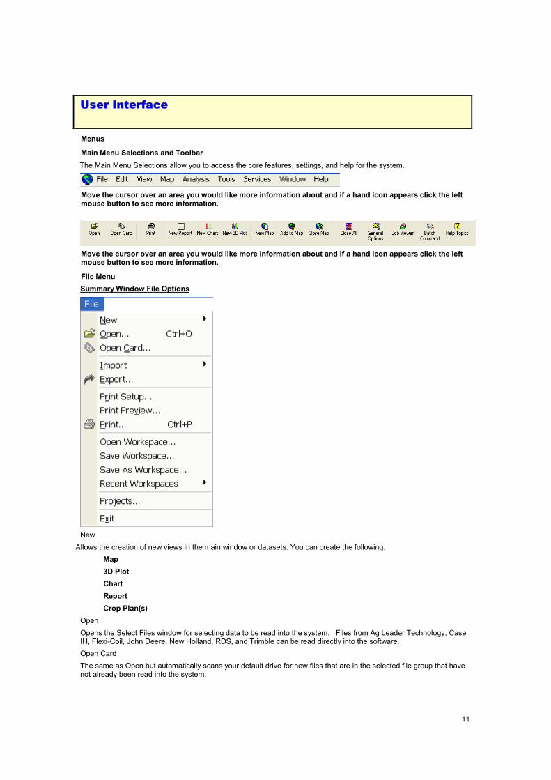
Main Menu Selections and ToolbarThe Main Menu Selections allow you to access the core features, settings, and help for the system.

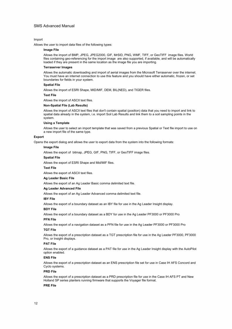
Move the cursor over an area you would like more information about and if a hand icon appears click the leftmouse button to see more information.


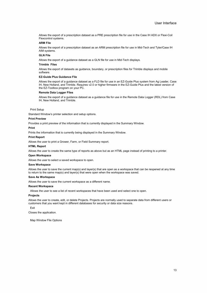
File MenuSummaryWindow File Options

NewAllows the creation of new views in the main window or datasets. You can create the following:

Map3D PlotChartReportCrop Plan(s)

OpenOpens the Select Files window for selecting data to be read into the system. Files from Ag Leader Technology, CaseIH, Flexi-Coil, John Deere, New Holland, RDS, and Trimble can be read directly into the software.Open CardThe same as Open but automatically scans your default drive for new files that are in the selected file group that havenot already been read into the system.

SMS Advanced Manual

12

ImportAllows the user to import data files of the following types:

Image FileAllows the import of BMP, JPEG, JPEG2000, GIF, MrSID, PNG, WMF, TIFF, or GeoTIFF image files. Worldfiles containing geo-referencing for the import image are also supported, if available, and will be automaticallyloaded if they are present in the same location as the image file you are importing.Terraserver ImagesAllows the automatic downloading and import of aerial images from the Microsoft Terraserver over the internet.You must have an internet connection to use this feature and you should have either automatic, frozen, or setboundaries for fields in your system.Spatial FileAllows the import of ESRI Shape, MID/MIF, DEM, BIL(NED), and TIGER files.Text FileAllows the import of ASCII text files.Non-Spatial File (Lab Results)Allows the import of ASCII text files that don't contain spatial (position) data that you need to import and link tospatial data already in the system, i.e. import Soil Lab Results and link them to a soil sampling points in thesystem.Using a TemplateAllows the user to select an import template that was saved from a previous Spatial or Text file import to use ona new import file of the same type.

ExportOpens the export dialog and allows the user to export data from the system into the following formats:

Image FileAllows the export of bitmap, JPEG, GIF, PNG, TIFF, or GeoTIFF image files.Spatial FileAllows the export of ESRI Shape and Mid/MIF files.Text FileAllows the export of ASCII text files.Ag Leader Basic FileAllows the export of an Ag Leader Basic comma delimited text file.Ag Leader Advanced FileAllows the export of an Ag Leader Advanced comma delimited text file.IBY FileAllows the export of a boundary dataset as an IBY file for use in the Ag Leader Insight display.BDY FileAllows the export of a boundary dataset as a BDY for use in the Ag Leader PF3000 or PF3000 ProPFN FileAllows the export of a navigation dataset as a PFN file for use in the Ag Leader PF3000 or PF3000 ProTGT FileAllows the export of a prescription dataset as a TGT prescription file for use in the Ag Leader PF3000, PF3000Pro, or Insight displays.PAT FileAllows the export of a guidance dataset as a PAT file for use in the Ag Leader Insight display with the AutoPilotoption enabled.ENS FileAllows the export of a prescription dataset as an ENS prescription file set for use in Case IH AFS Concord andCyclo systems.PRD FileAllows the export of a prescription dataset as a PRD prescription file for use in the Case IH AFS PT and NewHolland SP series planters running firmware that supports the Voyager file format.PRE File

User Interface

13

Allows the export of a prescription dataset as a PRE prescription file for use in the Case IH ADX or Flexi-CoilFlexcontrol systems.ARM FileAllows the export of a prescription dataset as an ARM prescription file for use in Mid-Tech and Tyler/Case IHAIM systems.GLN FileAllows the export of a guidance dataset as a GLN file for use in Mid-Tech displays.Trimble FilesAllows the export of datasets as guidance, boundary, or prescription files for Trimble displays and mobilesoftware.EZ-Guide Plus Guidance FileAllows the export of a guidance dataset as a FLD file for use in an EZ-Guide Plus system from Ag Leader, CaseIH, New Holland, and Trimble. Requires v2.0 or higher firmware in the EZ-Guide Plus and the latest version ofthe EZ-Toolbox program on your PC.Remote Data Logger FilesAllows the export of a guidance dataset as a guidance file for use in the Remote Data Logger (RDL) from CaseIH, New Holland, and Trimble.

Print SetupStandard Window�s printer selection and setup options.Print PreviewProvides a print preview of the information that is currently displayed in the Summary Window.PrintPrints the information that is currently being displayed in the Summary Window.Print ReportAllows the user to print a Grower, Farm, or Field Summary report.HTML ReportAllows the user to create the same type of reports as above but as an HTML page instead of printing to a printer.Open WorkspaceAllows the user to select a saved workspace to open.Save WorkspaceAllows the user to save the current map(s) and layer(s) that are open as a workspace that can be reopened at any timeto return to the same map(s) and layer(s) that were open when the workspace was saved.Save As WorkspaceAllows the user to save the current workspace as a different name.Recent WorkspaceAllows the user to see a list of recent workspaces that have been used and select one to open.ProjectsAllows the user to create, edit, or delete Projects. Projects are normally used to separate data from different users orcustomers that you want kept in different databases for security or data size reasons.ExitCloses the application.

Map Window File Options

SMS Advanced Manual

14

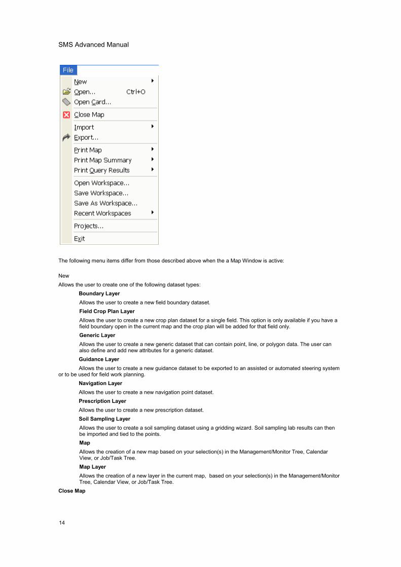
The following menu items differ from those described above when the a Map Window is active:

NewAllows the user to create one of the following dataset types:

Boundary LayerAllows the user to create a new field boundary dataset.Field Crop Plan LayerAllows the user to create a new crop plan dataset for a single field. This option is only available if you have afield boundary open in the current map and the crop plan will be added for that field only.Generic LayerAllows the user to create a new generic dataset that can contain point, line, or polygon data. The user canalso define and add new attributes for a generic dataset.Guidance LayerAllows the user to create a new guidance dataset to be exported to an assisted or automated steering system

or to be used for field work planning.Navigation LayerAllows the user to create a new navigation point dataset.Prescription LayerAllows the user to create a new prescription dataset.Soil Sampling LayerAllows the user to create a soil sampling dataset using a gridding wizard. Soil sampling lab results can thenbe imported and tied to the points.MapAllows the creation of a new map based on your selection(s) in the Management/Monitor Tree, CalendarView, or Job/Task Tree.Map LayerAllows the creation of a new layer in the current map, based on your selection(s) in the Management/MonitorTree, Calendar View, or Job/Task Tree.

Close Map

User Interface

15

Closes the Map that is currently active.Print MapThe following options are available for printing when a Map window is active:

Current LayerPrints a map of only the current layer.All LayersPrints a map printout for each layer that is open on individual pages.Current MapPrints a map of all open layers on one page and then each of the available layers information printed on thefollowing pages.Custom LayoutAllows the user to design a completely custom printout that can include such items as bitmaps and textdescriptions.

Print Map SummaryPrints a map summary report for the layers currently open in the active map.Print Query ResultsPrints a report of all the queries that have been performed in the active map.

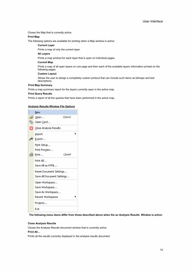
Analysis Results Window File Options

The following menu items differ from those described above when the an Analysis Results Window is active:

Close Analysis ResultsCloses the Analysis Results document window that is currently active.Print All...Prints all the results currently displayed in the analysis results document.

SMS Advanced Manual

16

Save All as HTML...Saves all the results currently displayed in the analysis results document as a single HTML file with links to eachanalysis result.Reset Document Settings...Select this option to clear any saved analysis document settings you have set back to the original defaults.Save All Document Settings...Select this option to save all the settings you have made for the current analysis result and analysis function that wasrun to generate them. When you rerun the same analysis function, these saved settings will be loaded to automaticallyformat your results the same way as when you saved. If you change the formatting or content of the results though, thesettings will automatically return to the default settings for your current results only.

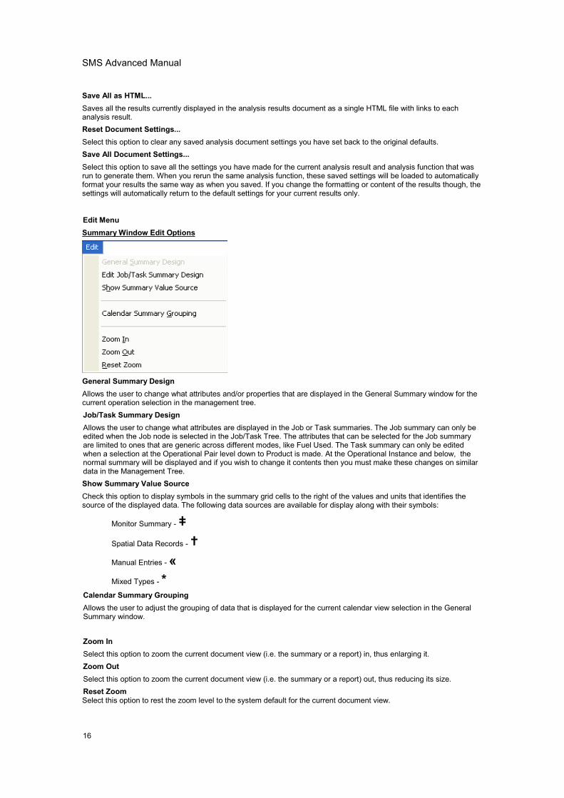
Edit MenuSummaryWindow Edit Options

General Summary DesignAllows the user to change what attributes and/or properties that are displayed in the General Summary window for thecurrent operation selection in the management tree.Job/Task Summary DesignAllows the user to change what attributes are displayed in the Job or Task summaries. The Job summary can only beedited when the Job node is selected in the Job/Task Tree. The attributes that can be selected for the Job summaryare limited to ones that are generic across different modes, like Fuel Used. The Task summary can only be editedwhen a selection at the Operational Pair level down to Product is made. At the Operational Instance and below, thenormal summary will be displayed and if you wish to change it contents then you must make these changes on similardata in the Management Tree.Show Summary Value SourceCheck this option to display symbols in the summary grid cells to the right of the values and units that identifies thesource of the displayed data. The following data sources are available for display along with their symbols:

Monitor Summary -�Spatial Data Records -�Manual Entries -�Mixed Types - *

Calendar Summary GroupingAllows the user to adjust the grouping of data that is displayed for the current calendar view selection in the GeneralSummary window.

Zoom InSelect this option to zoom the current document view (i.e. the summary or a report) in, thus enlarging it.Zoom OutSelect this option to zoom the current document view (i.e. the summary or a report) out, thus reducing its size.Reset ZoomSelect this option to rest the zoom level to the system default for the current document view.

User Interface

17

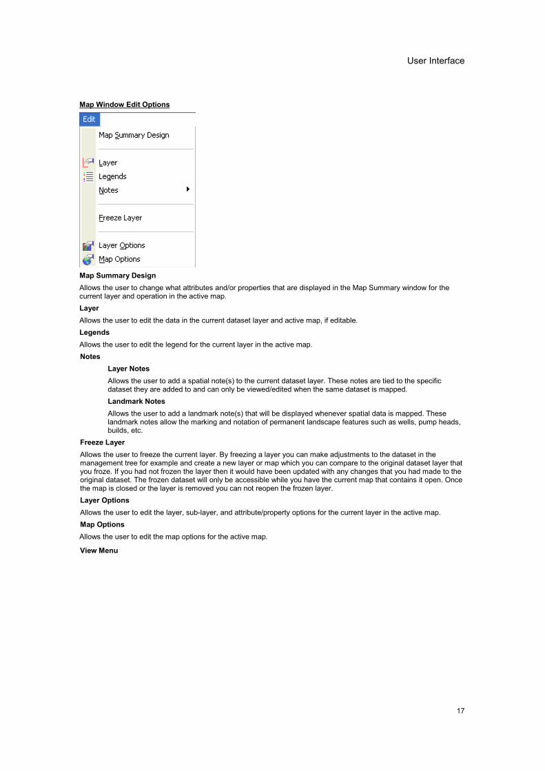
Map Window Edit Options

Map Summary DesignAllows the user to change what attributes and/or properties that are displayed in the Map Summary window for thecurrent layer and operation in the active map.LayerAllows the user to edit the data in the current dataset layer and active map, if editable.LegendsAllows the user to edit the legend for the current layer in the active map.Notes

Layer NotesAllows the user to add a spatial note(s) to the current dataset layer. These notes are tied to the specificdataset they are added to and can only be viewed/edited when the same dataset is mapped.Landmark NotesAllows the user to add a landmark note(s) that will be displayed whenever spatial data is mapped. Theselandmark notes allow the marking and notation of permanent landscape features such as wells, pump heads,builds, etc.

Freeze LayerAllows the user to freeze the current layer. By freezing a layer you can make adjustments to the dataset in themanagement tree for example and create a new layer or map which you can compare to the original dataset layer thatyou froze. If you had not frozen the layer then it would have been updated with any changes that you had made to theoriginal dataset. The frozen dataset will only be accessible while you have the current map that contains it open. Oncethe map is closed or the layer is removed you can not reopen the frozen layer.Layer OptionsAllows the user to edit the layer, sub-layer, and attribute/property options for the current layer in the active map.Map OptionsAllows the user to edit the map options for the active map.

View Menu

SMS Advanced Manual

18

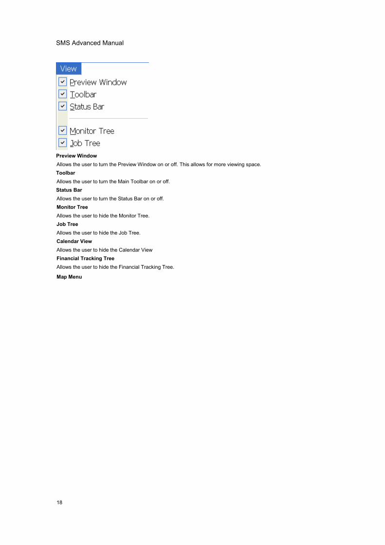
Preview WindowAllows the user to turn the Preview Window on or off. This allows for more viewing space.ToolbarAllows the user to turn the Main Toolbar on or off.Status BarAllows the user to turn the Status Bar on or off.Monitor TreeAllows the user to hide the Monitor Tree.Job TreeAllows the user to hide the Job Tree.Calendar ViewAllows the user to hide the Calendar ViewFinancial Tracking TreeAllows the user to hide the Financial Tracking Tree.

Map Menu

User Interface

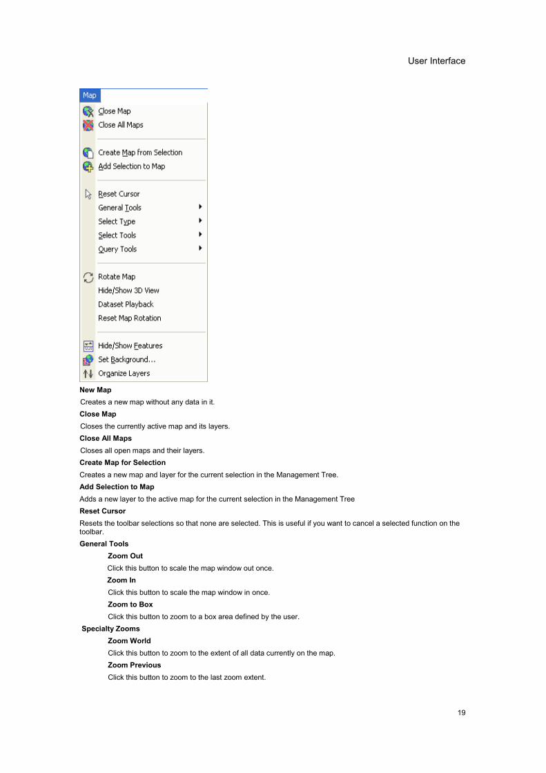
19

New MapCreates a new map without any data in it.Close MapCloses the currently active map and its layers.Close All MapsCloses all open maps and their layers.Create Map for SelectionCreates a new map and layer for the current selection in the Management Tree.Add Selection to MapAdds a new layer to the active map for the current selection in the Management TreeReset CursorResets the toolbar selections so that none are selected. This is useful if you want to cancel a selected function on thetoolbar.General Tools

Zoom OutClick this button to scale the map window out once.Zoom InClick this button to scale the map window in once.Zoom to BoxClick this button to zoom to a box area defined by the user.

Specialty ZoomsZoom WorldClick this button to zoom to the extent of all data currently on the map.Zoom PreviousClick this button to zoom to the last zoom extent.

SMS Advanced Manual

20

Zoom SelectionClick this button to zoom to the current layer selection.

PanAllows the user to drag the current contents of the map with the mouse in any direction.Line MeasureTape measure feature that allows the user to select a start and endpoint for a line and see the distance between thepoints.Multi-Line MeasureTape measure feature that allows the drawing of multiple, connected line segments and see a running total of overalldistance from the start of the first segment to the endpoint of the last one.Label Tools

Move LabelWhen User-Defined is selected on the Label Placement tab when editing Layer Options, this option willbecome active. When selected it allows the user to drag labels to any location on a map. To use click on anobject on the active layer that you want to move a label for and hold the mouse button down. The cursor willjump to the label location. Keep the mouse button held down and move the label to the desired location andthen release the mouse button.Label SettingsAllows the user to set various parameters for the display of labels for each object in a layer when User-Defined has been selected as the Label Placement type. Click on an object in the active layer to edit its labelproperties.

Select TypeSelect ObjectsWhen this selection type is selected, entire objects are selected when using one of the selection tools. Forexample if Select Polygon is selected and you draw a selection that crosses the edge of a polygon, the wholepolygon will be selected not just the intersected area.Select IntersectionsWhen this selection type is selected, only the intersected area of a n object is selected. For example if theSelect Polygon tool is selected and a region is drawn across a quarter of a line segment, then only that lengthof the line that fell in the selection area will be selected.

Select ToolsSelect PointAllows the user to select an individual spatial point.Select RectangleAllows the user to select a region with a box.Select PolygonAllows the user to select a region with a polygon.Select CircleAllows the user to select a region with a circle.Select EllipseAllows the user to select a region with an ellipse.Select PassAllows the user to select a pass. Only valid for point or smart rectangle map types.Select Via FilterAllows the user to select a region using data filters that the user defines. Data filters can be based on spatialstatistics, attributes, and properties and in combinations.

Query ToolsQuery Current LayerActivates the query feature for the current layer.Query through Current LayerActivates a query that cuts through all layers below the current layer, using the selected area as a "cookiecutter".Query Multiple Layers

User Interface

21

Activates the query feature for all layers that have been selected to be included in the multi-layer query.Select Query LayersAllows selection of all currently open layers in a map to be used in the multi-layer query.Clear Query ResultsClears all the query results from the Properties Window.

Rotate MapAllows the user to rotate the 3D view about the X, Y, and Z axis.Hide/Show 3D ViewAllows the user to toggle between displaying the current map in 2D or 3D view.Reset Map RotationAllows the user to reset the orientation and zoom level of the current 3D view to the default orientation.Dataset PlaybackAllows the user to start the Dataset Playback Viewer which maps the data in real-time based on the order, time-wise,that the data was logged.Hide or Show FeaturesAllows the user to either hide or show the Properties Window that is part of the Map Window.Set BackgroundAllows the user to select a background(s) to be viewed on the active map.Organize LayersAllows the user to reorder or delete layers in the active map.

Analysis menu

Analysis Wizard...Select this function to run the available analysis functions such as Attribute Comparison, Equation Writer, Multi-YearAggregate, etc.Multi-Project Analysis...Select this function to run either a Comparison or Correlation analysis across multiple projects that you select. This is avery powerful tool for generating regional analysis results from multiple users information.Spatial Data Finder...Select this function to build and/or run a dataset filter based on Management Items and/or Properties and thengenerate a new map or add a new layer(s) to an existing map based on the results. For example, you can run a filter tocreate a map of all the Grain Harvest datasets for a certain product such as all your corn harvest data.Financial Tracking EntriesSelect this function to enter detailed production financial values such as income, expenses, expense/income shares,etc.Financial Tracking ReportSelect this option to generate a non-spatial profit/loss report that represents all the financial entries that you havemade.

Tools Menu

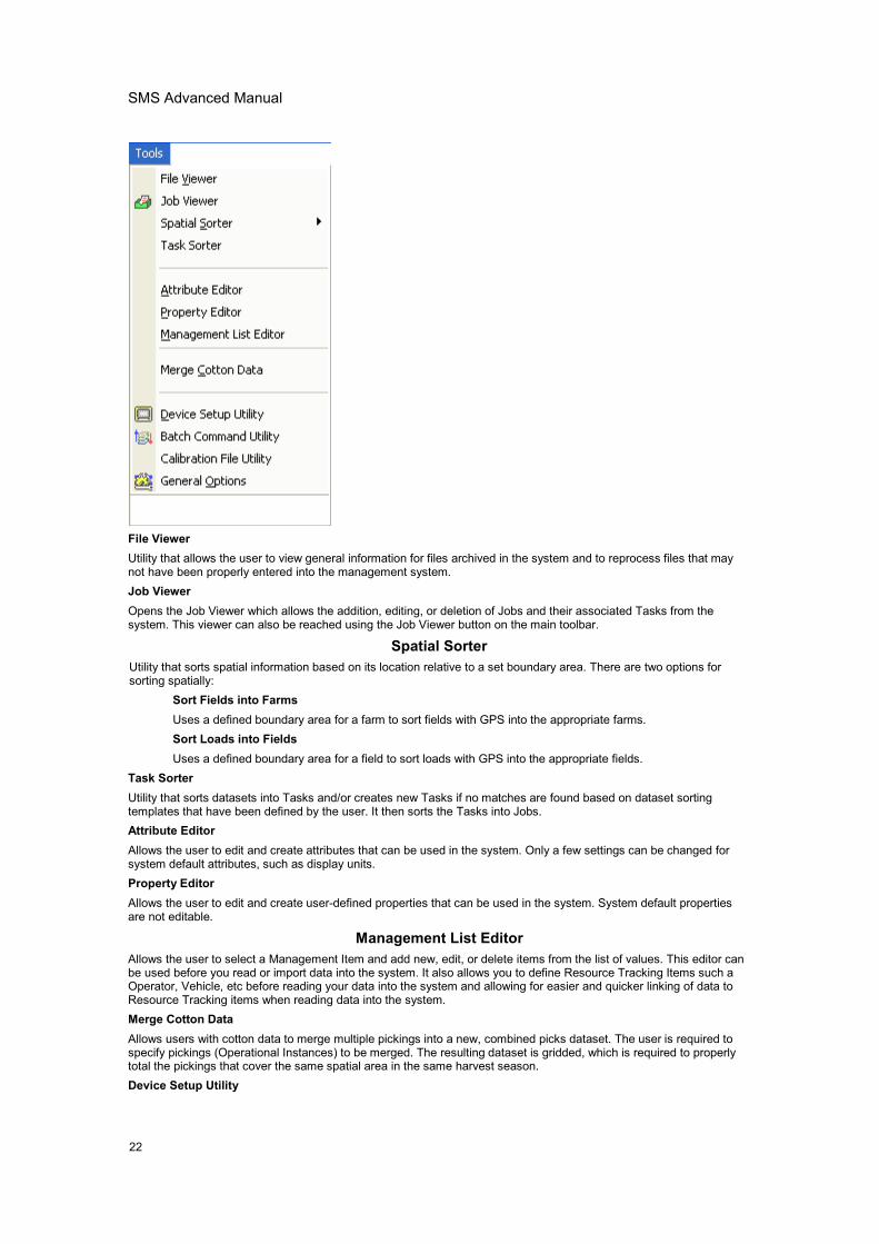
SMS Advanced Manual

22

File ViewerUtility that allows the user to view general information for files archived in the system and to reprocess files that maynot have been properly entered into the management system.Job ViewerOpens the Job Viewer which allows the addition, editing, or deletion of Jobs and their associated Tasks from thesystem. This viewer can also be reached using the Job Viewer button on the main toolbar.

Spatial SorterUtility that sorts spatial information based on its location relative to a set boundary area. There are two options forsorting spatially:

Sort Fields into FarmsUses a defined boundary area for a farm to sort fields with GPS into the appropriate farms.Sort Loads into FieldsUses a defined boundary area for a field to sort loads with GPS into the appropriate fields.

Task SorterUtility that sorts datasets into Tasks and/or creates new Tasks if no matches are found based on dataset sortingtemplates that have been defined by the user. It then sorts the Tasks into Jobs.Attribute EditorAllows the user to edit and create attributes that can be used in the system. Only a few settings can be changed forsystem default attributes, such as display units.Property EditorAllows the user to edit and create user-defined properties that can be used in the system. System default propertiesare not editable.

Management List EditorAllows the user to select a Management Item and add new, edit, or delete items from the list of values. This editor canbe used before you read or import data into the system. It also allows you to define Resource Tracking Items such aOperator, Vehicle, etc before reading your data into the system and allowing for easier and quicker linking of data toResource Tracking items when reading data into the system.Merge Cotton DataAllows users with cotton data to merge multiple pickings into a new, combined picks dataset. The user is required tospecify pickings (Operational Instances) to be merged. The resulting dataset is gridded, which is required to properlytotal the pickings that cover the same spatial area in the same harvest season.Device Setup Utility

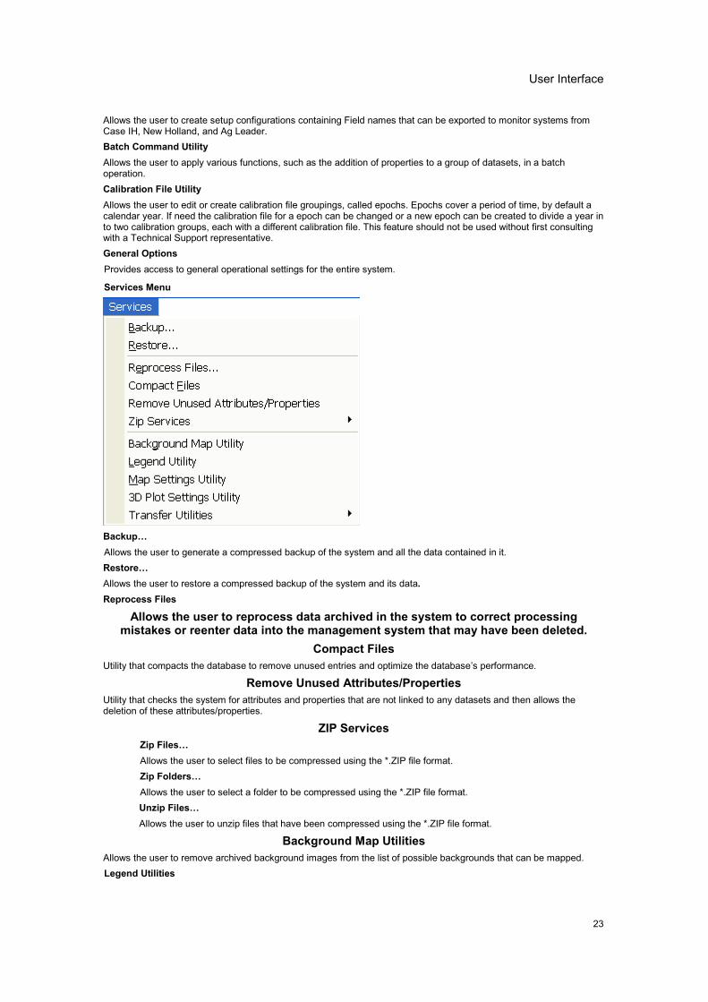
User Interface

23

Allows the user to create setup configurations containing Field names that can be exported to monitor systems fromCase IH, New Holland, and Ag Leader.Batch Command UtilityAllows the user to apply various functions, such as the addition of properties to a group of datasets, in a batchoperation.Calibration File UtilityAllows the user to edit or create calibration file groupings, called epochs. Epochs cover a period of time, by default acalendar year. If need the calibration file for a epoch can be changed or a new epoch can be created to divide a year into two calibration groups, each with a different calibration file. This feature should not be used without first consultingwith a Technical Support representative.General OptionsProvides access to general operational settings for the entire system.

Services Menu

Backup�Allows the user to generate a compressed backup of the system and all the data contained in it.Restore�Allows the user to restore a compressed backup of the system and its data.Reprocess Files

Allows the user to reprocess data archived in the system to correct processingmistakes or reenter data into the management system that may have been deleted.

Compact FilesUtility that compacts the database to remove unused entries and optimize the database�s performance.

Remove Unused Attributes/PropertiesUtility that checks the system for attributes and properties that are not linked to any datasets and then allows thedeletion of these attributes/properties.

ZIP ServicesZip Files�Allows the user to select files to be compressed using the *.ZIP file format.Zip Folders�Allows the user to select a folder to be compressed using the *.ZIP file format.Unzip Files�Allows the user to unzip files that have been compressed using the *.ZIP file format.

Background Map UtilitiesAllows the user to remove archived background images from the list of possible backgrounds that can be mapped.Legend Utilities

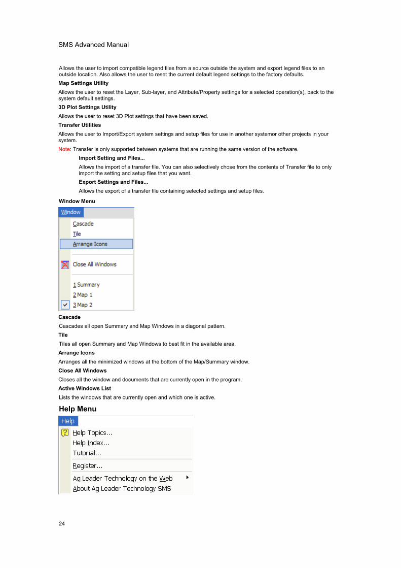
SMS Advanced Manual

24

Allows the user to import compatible legend files from a source outside the system and export legend files to anoutside location. Also allows the user to reset the current default legend settings to the factory defaults.Map Settings UtilityAllows the user to reset the Layer, Sub-layer, and Attribute/Property settings for a selected operation(s), back to thesystem default settings.3D Plot Settings UtilityAllows the user to reset 3D Plot settings that have been saved.Transfer UtilitiesAllows the user to Import/Export system settings and setup files for use in another systemor other projects in yoursystem.Note: Transfer is only supported between systems that are running the same version of the software.

Import Setting and Files...Allows the import of a transfer file. You can also selectively chose from the contents of Transfer file to onlyimport the setting and setup files that you want.Export Settings and Files...Allows the export of a transfer file containing selected settings and setup files.

Window Menu

CascadeCascades all open Summary and Map Windows in a diagonal pattern.TileTiles all open Summary and Map Windows to best fit in the available area.Arrange IconsArranges all the minimized windows at the bottom of the Map/Summary window.Close All WindowsCloses all the window and documents that are currently open in the program.Active Windows ListLists the windows that are currently open and which one is active.

Help Menu

User Interface

25

Help TopicsOpens the Table of Content for Help.Help IndexOpens the Index for Help.Tutorials�Opens the SMS Tutorial located on the SMS CD. The tutorial contains step by step descriptions and video for some ofthe more important functions in SMS.

Register�Allows the user to register their copy of SMS.

Ag Leader Technology on the WebProvides the user with links to web sites on the Internet. The following links are currently provided:

SMS Home PageProvides the user with a link to the main page for SMS on the Ag Leader Technology web site.SMS LinksProvides the user with a link to a page on the Ag Leader Technology web site that contains regularly updatedlinks to spatial data sources on the Internet that can be used in SMS Basic.Ag Leader Technology Home PageProvides a link to the main page of the Ag Leader Technology web site.

About ...Version and copyright information as well as a tool to check the system information for troubleshooting.

Main Windows

General LayoutThe layout of the main window is intended to help organize the large amounts of information that you will be storing,viewing, creating, editing, and analyzing. It�s also intended to reduce the learning curve associated with some otherprecision farming software packages by presenting a consistent and intuitive interface.

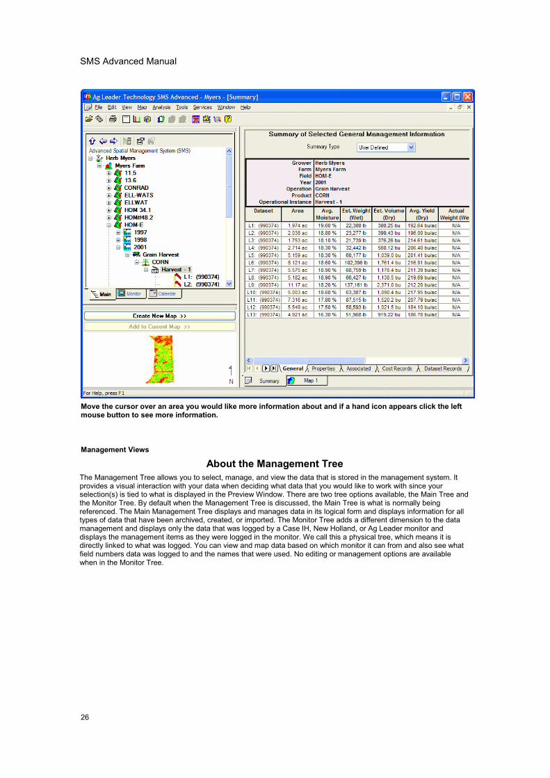
SMS Advanced Manual

26


Management Views

About the Management TreeThe Management Tree allows you to select, manage, and view the data that is stored in the management system. Itprovides a visual interaction with your data when deciding what data that you would like to work with since yourselection(s) is tied to what is displayed in the Preview Window. There are two tree options available, the Main Tree andthe Monitor Tree. By default when the Management Tree is discussed, the Main Tree is what is normally beingreferenced. The Main Management Tree displays and manages data in its logical form and displays information for alltypes of data that have been archived, created, or imported. The Monitor Tree adds a different dimension to the datamanagement and displays only the data that was logged by a Case IH, New Holland, or Ag Leader monitor anddisplays the management items as they were logged in the monitor. We call this a physical tree, which means it isdirectly linked to what was logged. You can view and map data based on which monitor it can from and also see whatfield numbers data was logged to and the names that were used. No editing or management options are availablewhen in the Monitor Tree.

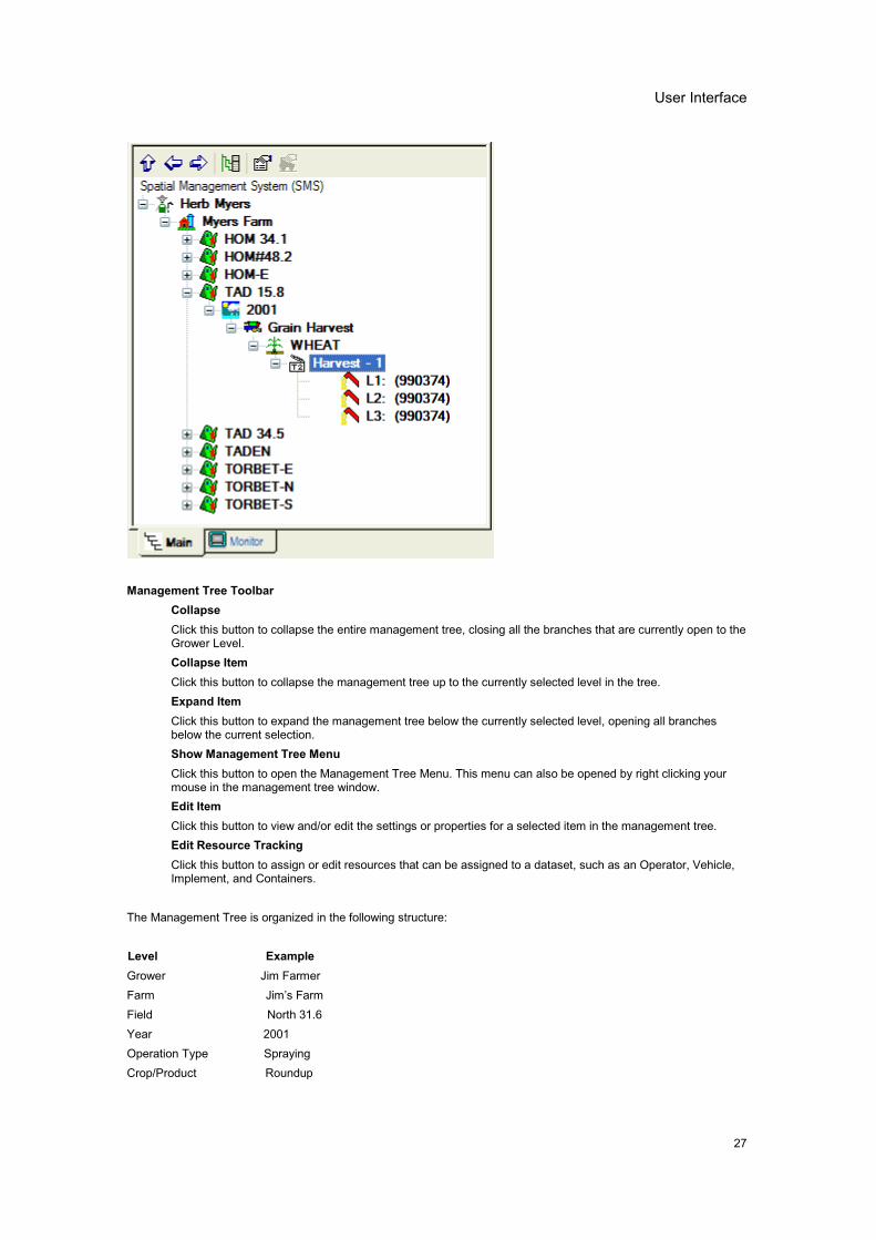
User Interface

27

Management Tree ToolbarCollapseClick this button to collapse the entire management tree, closing all the branches that are currently open to theGrower Level.Collapse ItemClick this button to collapse the management tree up to the currently selected level in the tree.Expand ItemClick this button to expand the management tree below the currently selected level, opening all branchesbelow the current selection.Show Management Tree MenuClick this button to open the Management Tree Menu. This menu can also be opened by right clicking yourmouse in the management tree window.Edit ItemClick this button to view and/or edit the settings or properties for a selected item in the management tree.Edit Resource TrackingClick this button to assign or edit resources that can be assigned to a dataset, such as an Operator, Vehicle,Implement, and Containers.

The Management Tree is organized in the following structure:

Level ExampleGrower Jim FarmerFarm Jim�s FarmField North 31.6Year 2001Operation Type SprayingCrop/Product Roundup

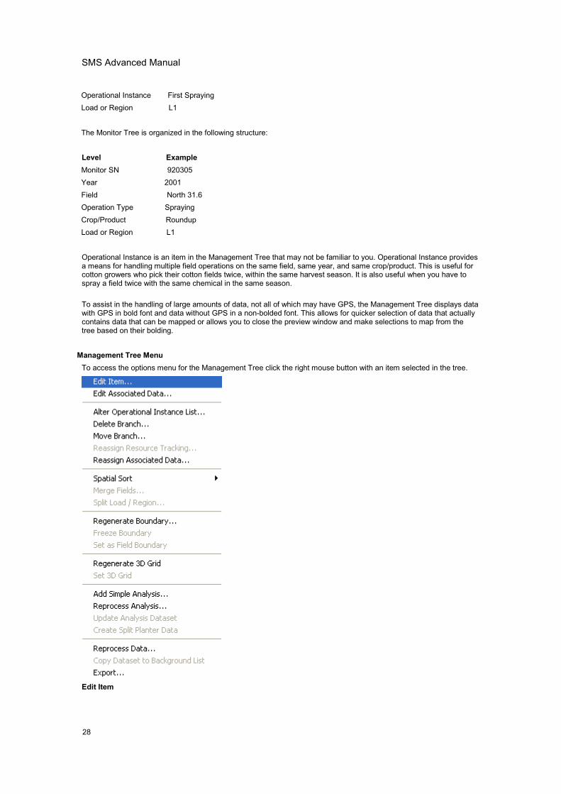
SMS Advanced Manual

28

Operational Instance First SprayingLoad or Region L1

The Monitor Tree is organized in the following structure:

Level ExampleMonitor SN 920305Year 2001Field North 31.6Operation Type SprayingCrop/Product RoundupLoad or Region L1

Operational Instance is an item in the Management Tree that may not be familiar to you. Operational Instance providesa means for handling multiple field operations on the same field, same year, and same crop/product. This is useful forcotton growers who pick their cotton fields twice, within the same harvest season. It is also useful when you have tospray a field twice with the same chemical in the same season.

To assist in the handling of large amounts of data, not all of which may have GPS, the Management Tree displays datawith GPS in bold font and data without GPS in a non-bolded font. This allows for quicker selection of data that actuallycontains data that can be mapped or allows you to close the preview window and make selections to map from thetree based on their bolding.

Management Tree MenuTo access the options menu for the Management Tree click the right mouse button with an item selected in the tree.

Edit Item

User Interface

29

Allows the user to view and/or edit the settings or properties for a selected item in the management tree.Edit Associated DataAllows the user to view, edit, or add an Associate dataset, such as a Scale Ticket or Note.Alter ListDisplays a list of all the logical items in the system for the selected item type. You can create, edit, or remove logicalitems from this dialog, even if they are not being used currently.Delete BranchDeletes the selected item and everything below it in the Management Tree. This does not remove archived data fromthe system, only the Management Tree information. Deleted items still remain in the system, to completely removethem use the Alter List� selection described above.Move BranchAllows the user to manually change the management settings for a selected item in the Management Tree.Reassign Resource TrackingAllows the user to assign or edit resources that can be assigned to a dataset, such as an Operator, Vehicle, Implement,and Containers.Reassign Associated DataAllows the user to edit the linkage of an Associated dataset to a management item(s) or remove it from the systemcompletely.Spatial SorterSorts spatial information based on its location relative to a set boundary area. Using this tool from the managementtree will only apply the sort to data that is below the current management level selection. Thus you can sort a selectedGrower or Farm only versus the Spatial Sort option located under the Tools menu which will sort all data in the system.There are two options for sorting spatially:

Sort Fields into FarmsUses a defined boundary area for a farm to sort fields with GPS into the appropriate farms.Sort Loads into FieldsUses a defined boundary area for a field to sort loads with GPS into the appropriate fields.

Merge FieldsAllows the merging of two logical fields into one. This option properly alters the data management for the merged fieldsso that any changes or new data that is read in will automatically apply to the merged location.Split Load /RegionAllows the user to split and sort a selected load/region into the appropriate spatial location even though it may havebeen logged improperly. Once a load/region is split, it can will not be updated with new data or recalibrated whenadjusted data files are read in. This option should only be used once all related data has been read into the systemand you are ready to place the data in the proper spatial location.Regenerate BoundaryRegenerates the automatic boundary area based on the selected dataset in the Management Tree. This will undo theFreeze Boundary� selection.Freeze BoundaryGenerates a vector boundary area for the selected automatic boundary area that the system generates. The vectorboundary area is required to use the Spatial Sorter.Set as Field BoundaryAllows the user to set a manually created or imported boundary or dataset as the Field boundary that is displayed.Regenerate 3D GridRegenerates the automatic 3D grid surface that is used to display a 3D terrain map of your data. By default thesoftware uses all the data read into the system to build the 3D grid surface but if errors are contained in some data thatis read in it may be necessary to pick only the data that contains good elevation data and use it to regenerate thesurface.Set 3D GridAllows the user to select an imported dataset that contains elevation, swath, and distance data in it to use as the 3Dgrid surface required for 3D mapping in place of the automatic 3D grid surface that the software generates. DEM(Digital Elevation Model)files are the most common file type that could be imported for this purpose, but any of thesupported import files could be used as long as they contain an Elevation, Swath Width, and Distance Attribute.Add Simple Analysis

SMS Advanced Manual

30

Allows the user to apply a simple analysis function to a dataset. Examples are Scale, Filter, and Normalize. Once asimple analysis function is applied to a dataset, it will be displayed in the management tree with a summation icon nextto it which indicates that a simple analysis function has been applied to the dataset, thus modifying it from its originalstate when it was read into the system.Reprocess AnalysisAllows the removal, editing, or addition of a simple analysis function for a selected dataset(s). Once all functions havebeen removed from a dataset, the raw values will again be displayed and accessible.Update Analysis DatasetAllows the updating of the data that was input into a full analysis function, such as Merge Cotton Data. If new data hasbeen read into the system that should be have been or needs to be applied to your analysis result, then selecting thisfunction will load the latest data available into the analysis function, re-run it automatically, and re-save the new resultdataset over the old data. This saves you the steps of having to manually delete the current analysis results from themanagement tree and then re-run the analysis function from scratch.Create Split Planter DataAllows the user to create split planter data from data that was not logged as such but was actually planted with a splitplanter configuration. This option can only be applied to Site Verification or Planting operation types and is onlyavailable when a dataset of this type is selected in the tree. By selecting the Operational Instance level in the tree, youcan create split planter data for all the loads/regions listed below the instance or by selecting individual loads/regions.There is also a batch function that allows you to create split planter data in bulk.Reprocess DataAllows the user to reprocess a selected dataset in the Management Tree. Depending on the dataset type, you will begiven options that can be changed or set to effect how the dataset is processed such as data filters and GPScorrections.Copy Dataset to Background ListAllows the user to copy a dataset from the Management Tree into the list of available backgrounds. This is very usefulif you've imported data that needed to be edited or that you decide you would just like to use as a background insteadof having it in the Management Tree.ExportAllows the export of data from the level that is currently selected in the Management Tree.

How to Information and Other Links:Using the Management TreeData Management

About the Job/Task TreeThe Job/Task Tree allows you to select, view, and edit Jobs and Tasks that you have created. A Job is defined as oneor more Tasks that you plan on occurring during a specified time span. A Task is defined as an operation(s) that youplan to occur in a specific field during a specified time span. Multiple Tasks can be added to a Job and multipleoperations can be set for a Task. An example would be that you make a Job for your spring planting. You add a Taskfor each field you plan to plant, set the Planned datasets for each field to the planting prescription for that field andleave the Actual datasets selection blank. After you plant your fields and read in the as-applied data, you can then linkthe actual planting data to the planting Task for each field. You then have a record of what you planned to do in eachfield and what actually happened. Jobs and Tasks also provide a very convenient and easy way to setup your devices(monitors) and export all the prescriptions that you wish to use, in one process, instead of exporting each fieldindividually. A summary of the Planned vs Actual values can also be seen based on selected levels in the Job/TaskTree.

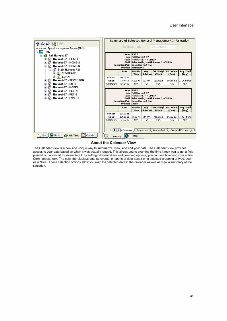
User Interface

31

About the Calendar ViewThe Calendar View is a new and unique way to summarize, view, and edit your data. The Calendar View providesaccess to your data based on when it was actually logged. This allows you to examine the time it took you to get a fieldplanted or harvested for example. Or by setting different filters and grouping options, you can see how long your entireCorn harvest took. The calendar displays data as events, or spans of data based on a selected grouping or type, suchas a Note. These selection options allow you map the selected data in the calendar as well as view a summary of theselection.

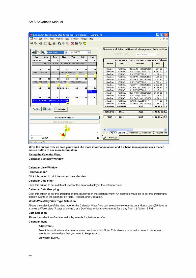
SMS Advanced Manual

32

Move the cursor over an area you would like more information about and if a hand icon appears click the leftmouse button to see more information.Using the Calendar View.Calendar SummaryWindow

Calendar View WindowPrint CalendarClick this button to print the current calendar view.Calendar Data FilterClick this button to set a dataset filter for the data to display in the calendar view.Calendar Data GroupingClick this button to set the grouping of data displayed in the calendar view. An example would be to set the grouping todisplay events in the calendar by Field, Product, and Operation.Month/Week/Day View Type SelectionAllows the selection of the view type for the Calendar View. You can select to view events on a Month basis(35 days ata time), a Week view (7 days at a time), or a Day View which shows events for a day from 12 AM to 12 PM.Date SelectionAllows the selection of a date to display events for, before, or after.Calendar Menu

Add Event...Select this option to add a manual event, such as a text Note. This allows you to make notes to documentevents on certain days that you want to keep track of.View/Edit Event...

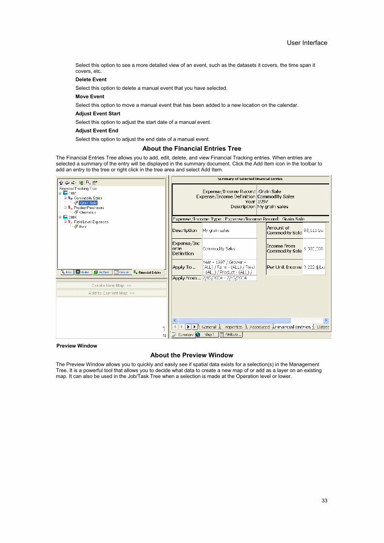
User Interface

33

Select this option to see a more detailed view of an event, such as the datasets it covers, the time span itcovers, etc.Delete EventSelect this option to delete a manual event that you have selected.Move EventSelect this option to move a manual event that has been added to a new location on the calendar.Adjust Event StartSelect this option to adjust the start date of a manual event.Adjust Event EndSelect this option to adjust the end date of a manual event.

About the Financial Entries TreeThe Financial Entries Tree allows you to add, edit, delete, and view Financial Tracking entries. When entries areselected a summary of the entry will be displayed in the summary document. Click the Add Item icon in the toolbar toadd an entry to the tree or right click in the tree area and select Add Item.

Preview Window

About the Preview WindowThe Preview Window allows you to quickly and easily see if spatial data exists for a selection(s) in the ManagementTree. It is a powerful tool that allows you to decide what data to create a new map of or add as a layer on an existingmap. It can also be used in the Job/Task Tree when a selection is made at the Operation level or lower.

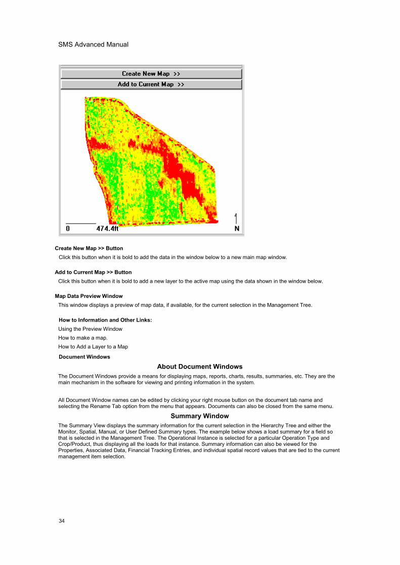
SMS Advanced Manual

34

Create New Map >> ButtonClick this button when it is bold to add the data in the window below to a new main map window.

Add to Current Map >> ButtonClick this button when it is bold to add a new layer to the active map using the data shown in the window below.

Map Data Preview WindowThis window displays a preview of map data, if available, for the current selection in the Management Tree.

How to Information and Other Links:Using the Preview WindowHow to make a map.How to Add a Layer to a Map

Document Windows

About Document WindowsThe Document Windows provide a means for displaying maps, reports, charts, results, summaries, etc. They are themain mechanism in the software for viewing and printing information in the system.

All Document Window names can be edited by clicking your right mouse button on the document tab name andselecting the Rename Tab option from the menu that appears. Documents can also be closed from the same menu.

Summary WindowThe Summary View displays the summary information for the current selection in the Hierarchy Tree and either theMonitor, Spatial, Manual, or User Defined Summary types. The example below shows a load summary for a field sothat is selected in the Management Tree. The Operational Instance is selected for a particular Operation Type andCrop/Product, thus displaying all the loads for that instance. Summary information can also be viewed for theProperties, Associated Data, Financial Tracking Entries, and individual spatial record values that are tied to the currentmanagement item selection.

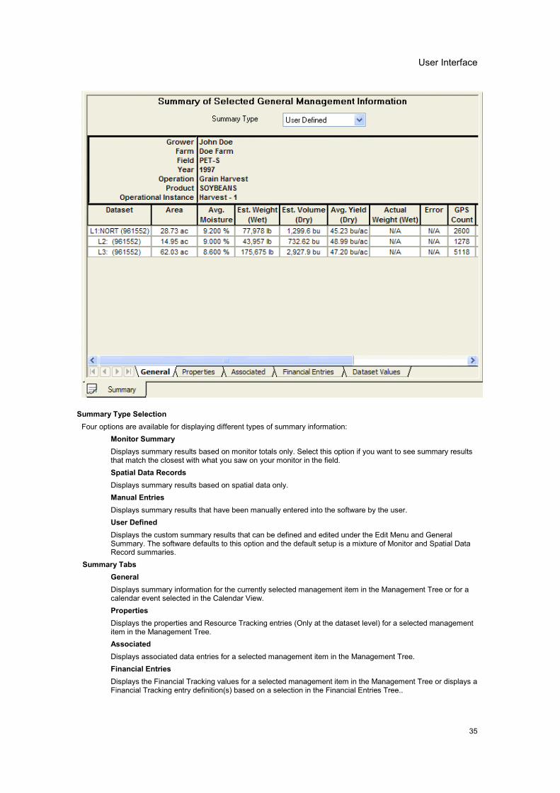
User Interface

35

Summary Type SelectionFour options are available for displaying different types of summary information:

Monitor SummaryDisplays summary results based on monitor totals only. Select this option if you want to see summary resultsthat match the closest with what you saw on your monitor in the field.Spatial Data RecordsDisplays summary results based on spatial data only.Manual EntriesDisplays summary results that have been manually entered into the software by the user.User DefinedDisplays the custom summary results that can be defined and edited under the Edit Menu and GeneralSummary. The software defaults to this option and the default setup is a mixture of Monitor and Spatial DataRecord summaries.

Summary TabsGeneralDisplays summary information for the currently selected management item in the Management Tree or for acalendar event selected in the Calendar View.PropertiesDisplays the properties and Resource Tracking entries (Only at the dataset level) for a selected managementitem in the Management Tree.AssociatedDisplays associated data entries for a selected management item in the Management Tree.Financial EntriesDisplays the Financial Tracking values for a selected management item in the Management Tree or displays aFinancial Tracking entry definition(s) based on a selection in the Financial Entries Tree..

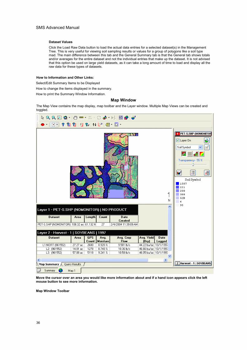
SMS Advanced Manual

36

Dataset ValuesClick the Load Raw Data button to load the actual data entries for a selected dataset(s) in the ManagementTree. This is very useful for viewing soil sampling results or values for a group of polygons like a soil typemad. The main difference between this tab and the General Summary tab is that the General tab shows totalsand/or averages for the entire dataset and not the individual entries that make up the dataset. It is not advisedthat this option be used on large yield datasets, as it can take a long amount of time to load and display all theraw data for these types of datasets.

How to Information and Other Links:Select/Edit Summary Items to be DisplayedHow to change the items displayed in the summary.How to print the Summary Window Information.

Map WindowThe Map View contains the map display, map toolbar and the Layer window. Multiple Map Views can be created andtoggled.


Map Window Toolbar

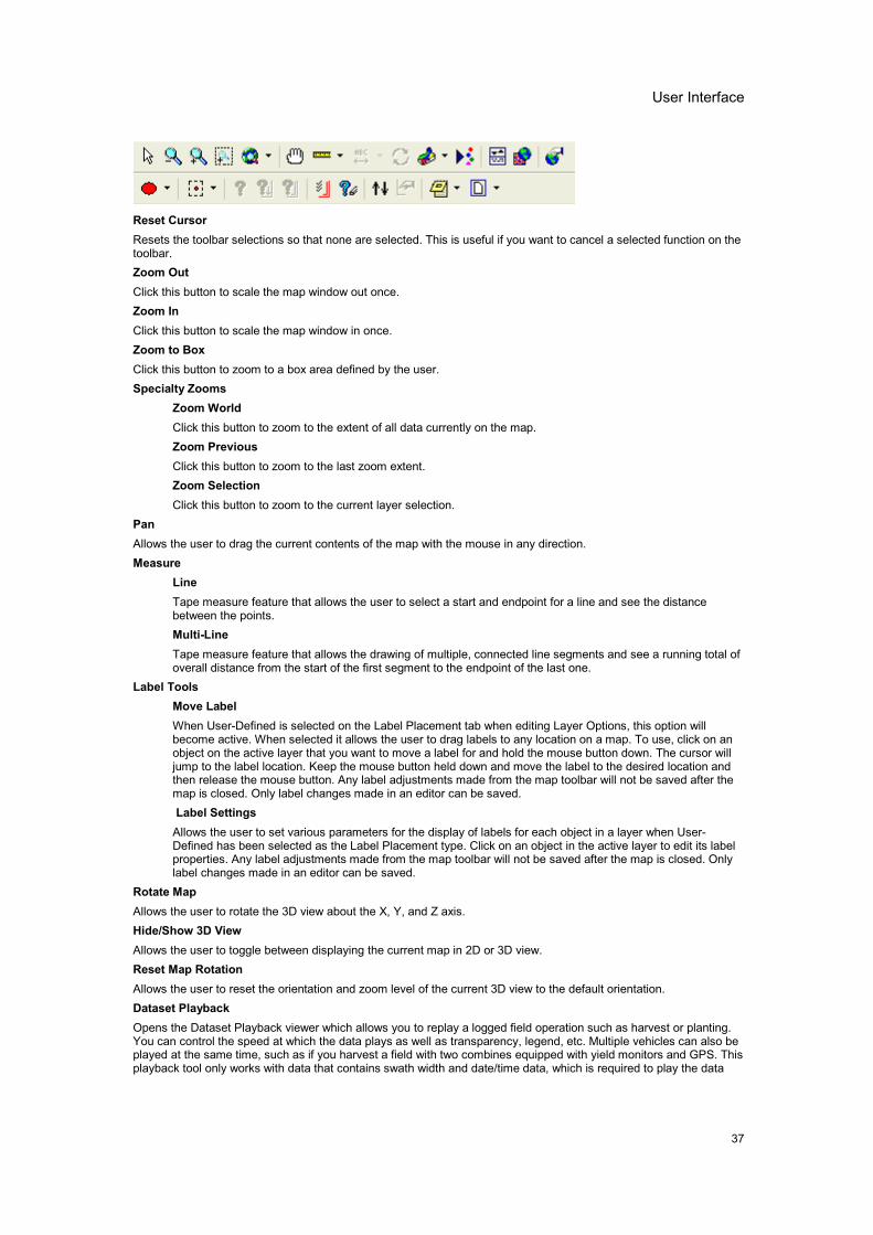
User Interface

37

Reset CursorResets the toolbar selections so that none are selected. This is useful if you want to cancel a selected function on thetoolbar.Zoom OutClick this button to scale the map window out once.Zoom InClick this button to scale the map window in once.Zoom to BoxClick this button to zoom to a box area defined by the user.Specialty Zooms

Zoom WorldClick this button to zoom to the extent of all data currently on the map.Zoom PreviousClick this button to zoom to the last zoom extent.Zoom SelectionClick this button to zoom to the current layer selection.

PanAllows the user to drag the current contents of the map with the mouse in any direction.Measure

LineTape measure feature that allows the user to select a start and endpoint for a line and see the distancebetween the points.Multi-LineTape measure feature that allows the drawing of multiple, connected line segments and see a running total ofoverall distance from the start of the first segment to the endpoint of the last one.

Label ToolsMove LabelWhen User-Defined is selected on the Label Placement tab when editing Layer Options, this option willbecome active. When selected it allows the user to drag labels to any location on a map. To use, click on anobject on the active layer that you want to move a label for and hold the mouse button down. The cursor willjump to the label location. Keep the mouse button held down and move the label to the desired location andthen release the mouse button. Any label adjustments made from the map toolbar will not be saved after themap is closed. Only label changes made in an editor can be saved.Label SettingsAllows the user to set various parameters for the display of labels for each object in a layer when User-Defined has been selected as the Label Placement type. Click on an object in the active layer to edit its labelproperties. Any label adjustments made from the map toolbar will not be saved after the map is closed. Onlylabel changes made in an editor can be saved.

Rotate MapAllows the user to rotate the 3D view about the X, Y, and Z axis.Hide/Show 3D ViewAllows the user to toggle between displaying the current map in 2D or 3D view.Reset Map RotationAllows the user to reset the orientation and zoom level of the current 3D view to the default orientation.Dataset PlaybackOpens the Dataset Playback viewer which allows you to replay a logged field operation such as harvest or planting.You can control the speed at which the data plays as well as transparency, legend, etc. Multiple vehicles can also beplayed at the same time, such as if you harvest a field with two combines equipped with yield monitors and GPS. Thisplayback tool only works with data that contains swath width and date/time data, which is required to play the data

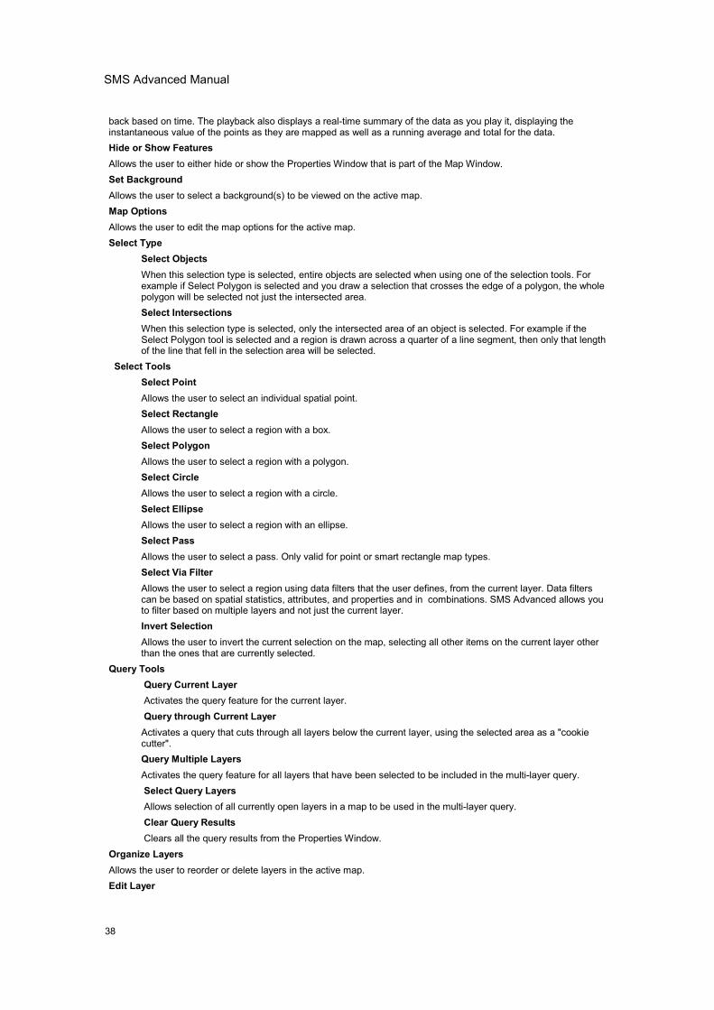
SMS Advanced Manual

38

back based on time. The playback also displays a real-time summary of the data as you play it, displaying theinstantaneous value of the points as they are mapped as well as a running average and total for the data.Hide or Show FeaturesAllows the user to either hide or show the Properties Window that is part of the Map Window.Set BackgroundAllows the user to select a background(s) to be viewed on the active map.Map OptionsAllows the user to edit the map options for the active map.Select Type

Select ObjectsWhen this selection type is selected, entire objects are selected when using one of the selection tools. Forexample if Select Polygon is selected and you draw a selection that crosses the edge of a polygon, the wholepolygon will be selected not just the intersected area.Select IntersectionsWhen this selection type is selected, only the intersected area of an object is selected. For example if theSelect Polygon tool is selected and a region is drawn across a quarter of a line segment, then only that lengthof the line that fell in the selection area will be selected.

Select ToolsSelect PointAllows the user to select an individual spatial point.Select RectangleAllows the user to select a region with a box.Select PolygonAllows the user to select a region with a polygon.Select CircleAllows the user to select a region with a circle.Select EllipseAllows the user to select a region with an ellipse.Select PassAllows the user to select a pass. Only valid for point or smart rectangle map types.Select Via FilterAllows the user to select a region using data filters that the user defines, from the current layer. Data filterscan be based on spatial statistics, attributes, and properties and in combinations. SMS Advanced allows youto filter based on multiple layers and not just the current layer.Invert SelectionAllows the user to invert the current selection on the map, selecting all other items on the current layer otherthan the ones that are currently selected.

Query ToolsQuery Current LayerActivates the query feature for the current layer.Query through Current LayerActivates a query that cuts through all layers below the current layer, using the selected area as a "cookiecutter".Query Multiple LayersActivates the query feature for all layers that have been selected to be included in the multi-layer query.Select Query LayersAllows selection of all currently open layers in a map to be used in the multi-layer query.Clear Query ResultsClears all the query results from the Properties Window.

Organize LayersAllows the user to reorder or delete layers in the active map.Edit Layer

User Interface

39

Allows the user to edit the current layer in the active map if it is editable.Notes

Layer NotesAllows the user to add a spatial note(s) to the current dataset layer. These notes are tied to the specificdataset they are added to and can only be viewed/edited when the same dataset is mapped.Landmark NotesAllows the user to add a landmark note(s) that will be displayed whenever spatial data is mapped. Theselandmark notes allow the marking and notation of permanent landscape features such as wells, pump heads,builds, etc.

NewAllows the user to create one of the following file types:

Boundary MapAllows the user to create a new boundary dataset for the current layer in the active map.GenericAllows the user to create a new generic dataset that can contain point, line, or polygon data. The user canalso define and add new attributes for a generic dataset.Navigation MapAllows the user to create a new navigation dataset for the current layer in the active map.Prescription MapAllows the user to create a new prescription dataset for the active map.Soil Sampling MapAllows the user to create a soil sampling dataset using a gridding wizard. Soil sampling lab results can thenbe imported and tied to the points.

How to Information and Other Links:MappingHow to make a map.How to Add a Layer to a Map

Map Properties TabsProperties for the map that is currently selected can be displayed by clicking the Hide/Show Properties icon on theMap Toolbar or by selecting Hide/Show Properties in the Map Menu. Map Summary and Query Results tabs areselectable when this option is selected, and the map window splits to show the map on the top and the map propertiesbelow it. The percentage of the window used by the map or the properties can be adjusted vertically by left clicking onthe bar that separates the two, holding it down, and then dragging the bar up and down until the desired sizing isreached.

Select one of the topics below for more information:Map Summary ViewQuery Results View

3D Plot WindowThe 3D Plot document window displays a 3D plot of a selected dataset from the Management Tree. It provides varioustools and settings for manipulating and displaying the 3D Plot. The 3D Plot can also be printed.

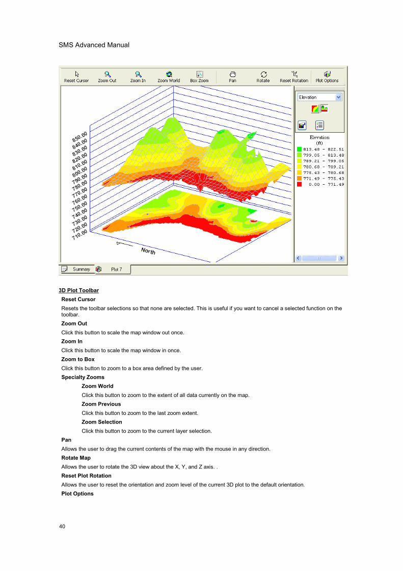
SMS Advanced Manual

40

3D Plot ToolbarReset CursorResets the toolbar selections so that none are selected. This is useful if you want to cancel a selected function on thetoolbar.Zoom OutClick this button to scale the map window out once.Zoom InClick this button to scale the map window in once.Zoom to BoxClick this button to zoom to a box area defined by the user.Specialty Zooms

Zoom WorldClick this button to zoom to the extent of all data currently on the map.Zoom PreviousClick this button to zoom to the last zoom extent.Zoom SelectionClick this button to zoom to the current layer selection.

PanAllows the user to drag the current contents of the map with the mouse in any direction.Rotate MapAllows the user to rotate the 3D view about the X, Y, and Z axis. .Reset Plot RotationAllows the user to reset the orientation and zoom level of the current 3D plot to the default orientation.Plot Options

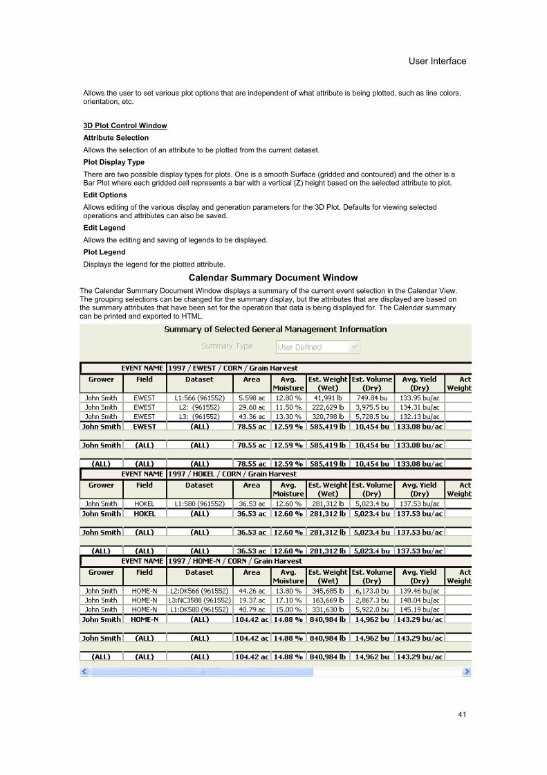
User Interface

41

Allows the user to set various plot options that are independent of what attribute is being plotted, such as line colors,orientation, etc.

3D Plot Control WindowAttribute SelectionAllows the selection of an attribute to be plotted from the current dataset.Plot Display TypeThere are two possible display types for plots. One is a smooth Surface (gridded and contoured) and the other is aBar Plot where each gridded cell represents a bar with a vertical (Z) height based on the selected attribute to plot.Edit OptionsAllows editing of the various display and generation parameters for the 3D Plot. Defaults for viewing selectedoperations and attributes can also be saved.Edit LegendAllows the editing and saving of legends to be displayed.Plot LegendDisplays the legend for the plotted attribute.

Calendar Summary Document WindowThe Calendar Summary Document Window displays a summary of the current event selection in the Calendar View.The grouping selections can be changed for the summary display, but the attributes that are displayed are based onthe summary attributes that have been set for the operation that data is being displayed for. The Calendar summarycan be printed and exported to HTML.

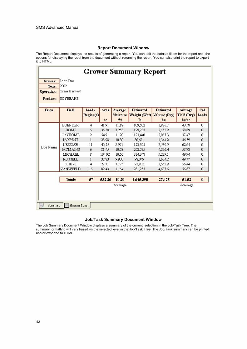
SMS Advanced Manual

42

Report Document WindowThe Report Document displays the results of generating a report. You can edit the dataset filters for the report and theoptions for displaying the repot from the document without rerunning the report. You can also print the report to exportit to HTML.

Job/Task Summary Document WindowThe Job Summary Document Window displays a summary of the current selection in the Job/Task Tree. Thesummary formatting will vary based on the selected level in the Job/Task Tree. The Job/Task summary can be printedand/or exported to HTML.

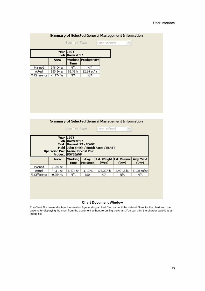
User Interface

43

Chart Document WindowThe Chart Document displays the results of generating a chart. You can edit the dataset filters for the chart and theoptions for displaying the chart from the document without rerunning the chart .You can print the chart or save it as animage file.

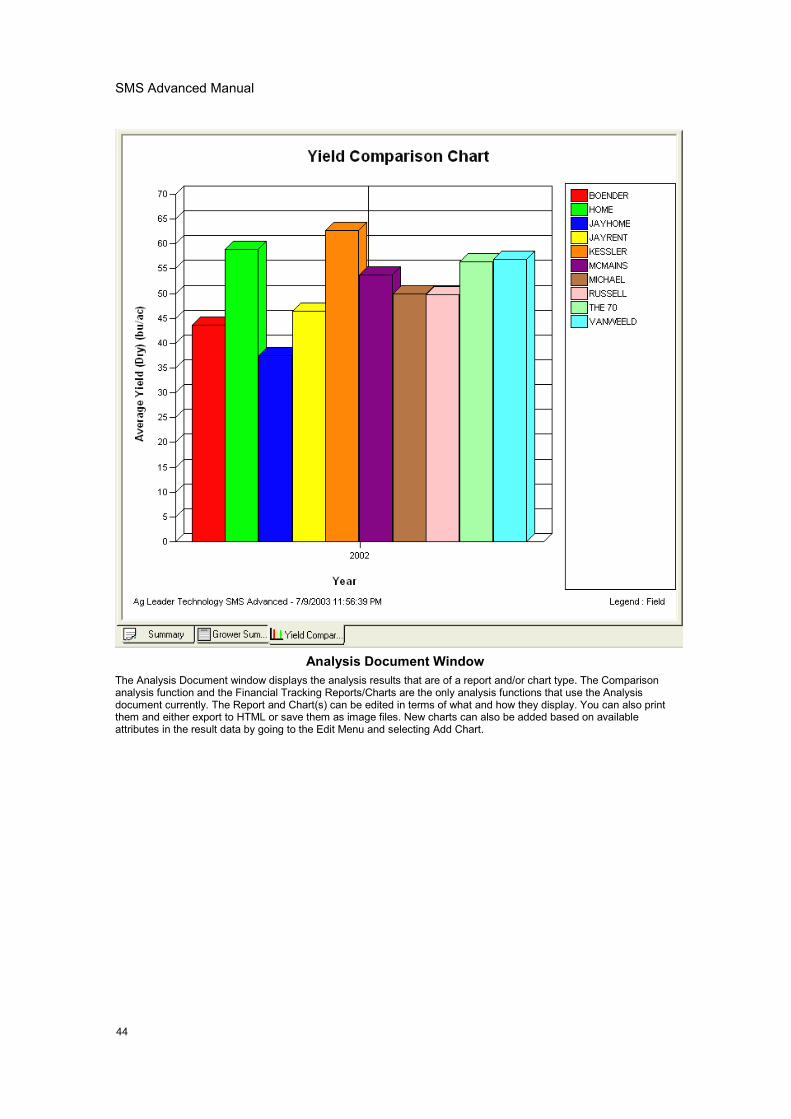
SMS Advanced Manual

44

Analysis Document WindowThe Analysis Document window displays the analysis results that are of a report and/or chart type. The Comparisonanalysis function and the Financial Tracking Reports/Charts are the only analysis functions that use the Analysisdocument currently. The Report and Chart(s) can be edited in terms of what and how they display. You can also printthem and either export to HTML or save them as image files. New charts can also be added based on availableattributes in the result data by going to the Edit Menu and selecting Add Chart.

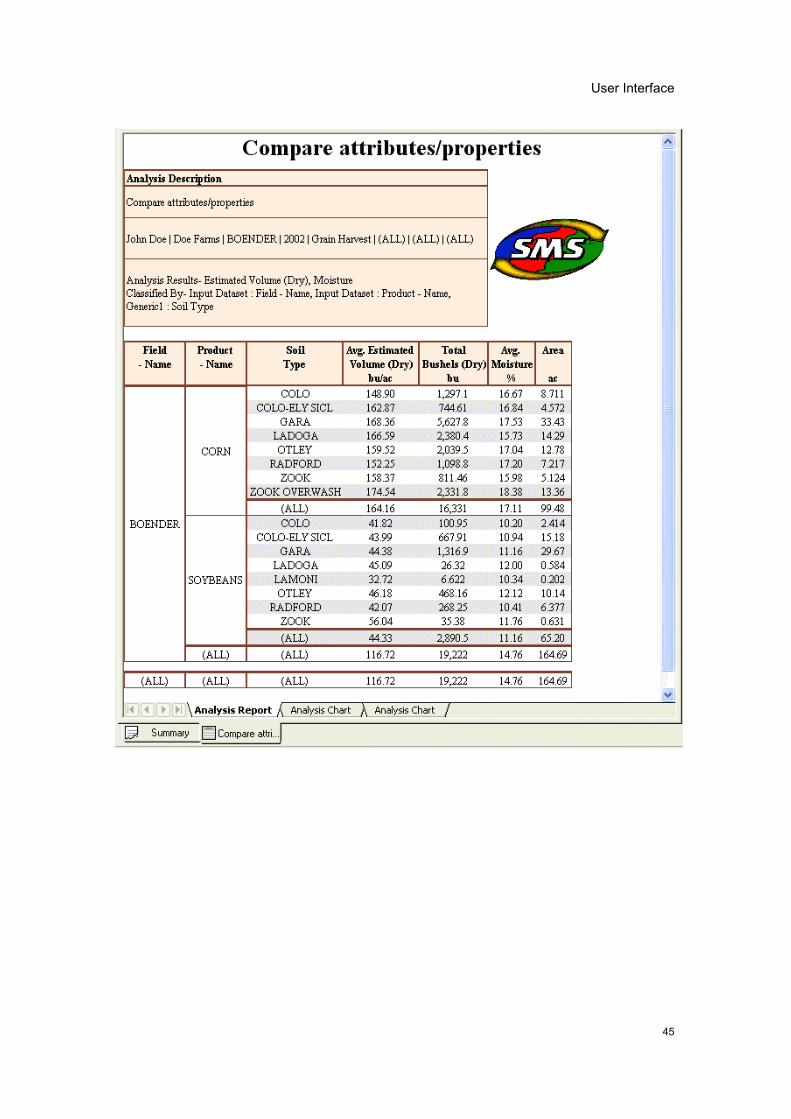
User Interface

45

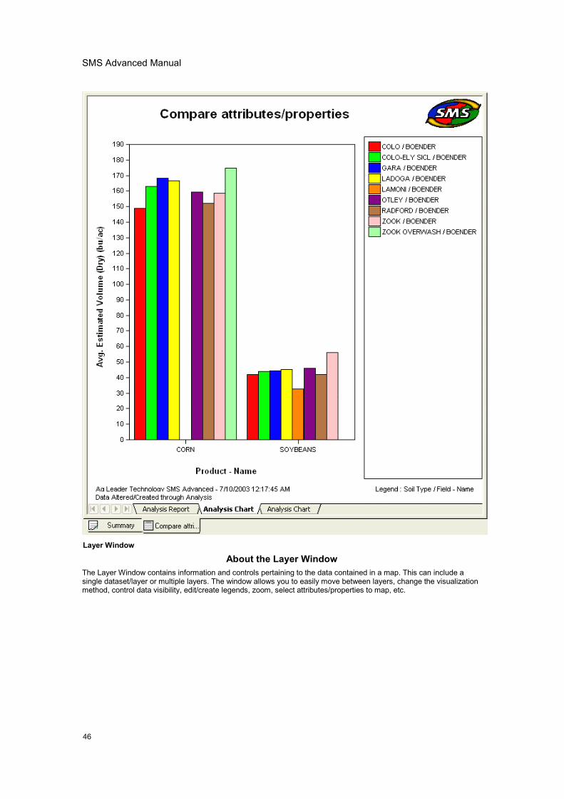
SMS Advanced Manual

46

Layer Window

About the Layer WindowThe Layer Window contains information and controls pertaining to the data contained in a map. This can include asingle dataset/layer or multiple layers. The window allows you to easily move between layers, change the visualizationmethod, control data visibility, edit/create legends, zoom, select attributes/properties to map, etc.

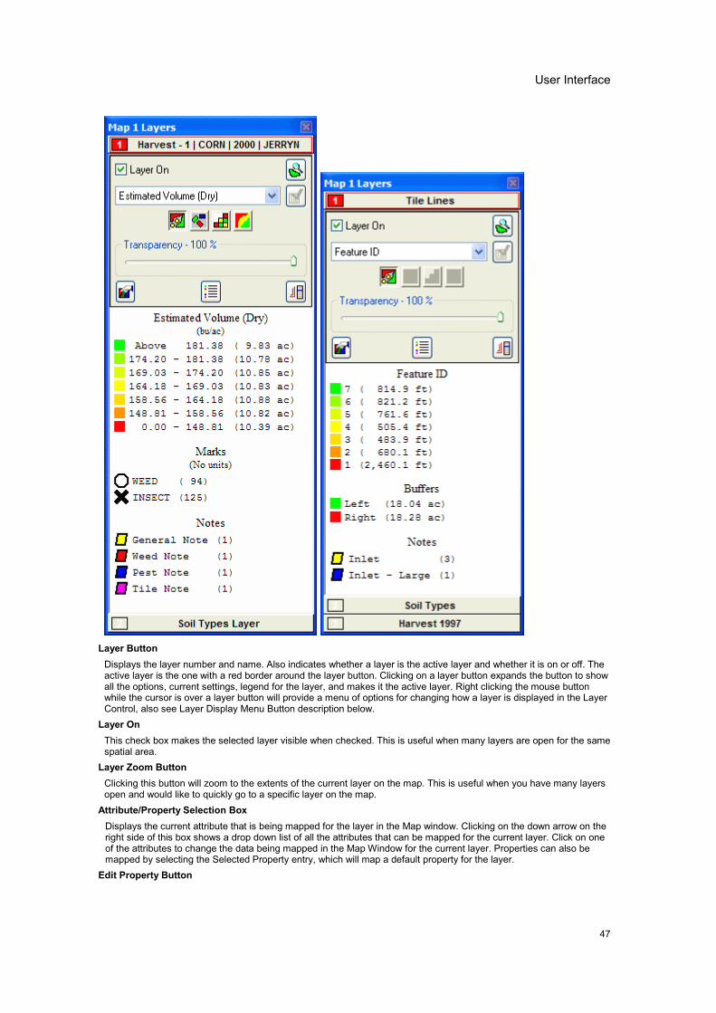
User Interface

47

Layer ButtonDisplays the layer number and name. Also indicates whether a layer is the active layer and whether it is on or off. Theactive layer is the one with a red border around the layer button. Clicking on a layer button expands the button to showall the options, current settings, legend for the layer, and makes it the active layer. Right clicking the mouse buttonwhile the cursor is over a layer button will provide a menu of options for changing how a layer is displayed in the LayerControl, also see Layer Display Menu Button description below.Layer OnThis check box makes the selected layer visible when checked. This is useful when many layers are open for the samespatial area.Layer Zoom ButtonClicking this button will zoom to the extents of the current layer on the map. This is useful when you have many layersopen and would like to quickly go to a specific layer on the map.Attribute/Property Selection BoxDisplays the current attribute that is being mapped for the layer in the Map window. Clicking on the down arrow on theright side of this box shows a drop down list of all the attributes that can be mapped for the current layer. Click on oneof the attributes to change the data being mapped in the Map Window for the current layer. Properties can also bemapped by selecting the Selected Property entry, which will map a default property for the layer.Edit Property Button

SMS Advanced Manual

48

Click this button when Select Property is selected in the Attribute/Property Selection Box to set the current propertythat will be mapped for the active layer.Swath Selection BoxDisplays the current swath representation in the Map Window. This currently is defaulted to Full Swath for all datatypes except for Cotton Harvest data which allows the user to select Full Swath, All Swath Segments, or individualswath segments that data was collected for.Map Type ButtonsThese five button change the way that data is displayed in the Map Window.Spatial Map

Creates a raw data map of a spatial dataset.Smart Rectangle MapCreates a map based on spatial points plotted as rectangular objects that are created from the swath width,distance traveled and heading (track) for the logged point. Track must be included in the dataset beingmapped to display the data as smart rectangles.Grid MapCreates a map based on averaged values for a user set grid size. See Edit Layer Options.Contour MapCreates a map based on averaged and smoothed values for a user set grid size. See Edit Layer Options.

Transparency Slider BarSets the transparency level of the current layer and attribute to a value from 10 to 100 percent, 100 percent beingcompletely solid.Edit Layer Options ButtonClick this button to go to the Layer and Attribute/Property Options Dialog. Allows the user to edit the layer, sub-layer,and attribute/property options for the current layer in the active map. This includes setting whether marks are turnedon or off, point diameter size, grid size, properties for spatial datasets, contour parameters, etc..Edit Legend ButtonClicking this button opens the Edit Legend Dialog. This allows you set the various parameters for the legend, marks,and view statistical information for the layer.Layer Display Menu ButtonClicking this button displays a menu of options that modify how a layer is displayed in the Layer Window, such asmoving layers up/down, renaming them, or removing them.Legend AreaDisplays the legend for the current layer and selected attribute. Also displays the legend for marks, buffers, and layernotes data if present. Double clicking with the left mouse button in the legend area will open the Edit Legend dialog.

How to Information and Other Links:Edit LegendUsing the Layer WindowHow to edit a legend.

49

��

Processing DataThe software provides a number of options for processing the data you are reading into the system or data already inthe system. The software allows you to set processing settings for the particular type of data and the product/crop thatdata was collected for as well as settings for GPS position data correction and filtering.Select one of the following topics below on processing data and files:Open File or CardSelect ManagementArchiving OptionsManagement and Processing Settings

Processing New DataThe software provides a wizard interface for reading Ag Leader, Case IH, Flexi-Coil, JD Greenstar, Mid-Tech, NewHolland, RDS , and Trimble files into the system. This wizard interface greatly simplifies entering your files into thesystem.

How to read Ag Leader, Case IH, JD Greenstar, RDS, New Holland, Mid-Tech, or Flexi-Coil files into the system.How to migrate your data from Precision Map 2000 or Instant Yield Map Software

Reprocessing Data Already in the SystemOnce data that supports reprocessing has been read into the system, you have the option to reprocess the data tomake changes to the data that is displayed when you create a map(s) or layer(s).How to reprocess data.

Reprocessing Files that have Already Been Read into the SystemIf you delete files from the Management Tree using the Delete Branch selection, the proper way to get the deleted databack into the system is to use the Reprocess Files�selection under the Services menu. The reason this is thepreferred method is that the software does not allow duplicate files to be read into the Data Vault where all the files youread in are stored. Since the file has already been read into the system once, this feature allows you to select filesalready in the vault and reprocess them. Please note that this tool should not be used to adjust processing settings fordata already in the system, use Reprocess Data..under the Management Tree Menu to do that.Reprocess Files

51

��

Data ManagementThe software provides a number of different methods and tools for ensuring that your data is managed properly. Theseinclude automatic management features like the Spatial Sorter or manually setting the management settings for anitem in the Management Tree such as a Field.

NOTE: Do not remove any files, such as YLD�s, from the system Data Vault. Doing so may cause unexpectedresults such as not being able to map data in the system or read in new files. Files stored in the vault arelinked to other data files within the system or database. Removing these files will cause problems for otheritems in the system that are referenced to them. Please contact Technical Support for assistance in removingdata files from the system properly. In general, do not delete any files from the system Data directory withoutfirst consulting with Technical Support.

Select one of the topics below on data management in the system:Select ManagementLogical Management Item ListApply Management ChangesArchiving OptionsReassign Resource TrackingReassign Associated Data

Managing FarmsHow to manually move a FarmHow to spatially sort Fields into Farms.

Managing FieldsMerge FieldsHow to freeze a boundary.How to spatially sort Loads/Regions into Fields.How to split and sort a load or region.How to manually move a Field.

Managing Other Items in the Management TreeHow to manually move other management items (Year, Load, etc.).

WorkspacesThe software allows you to save and open Workspaces. A workspace is like a bookmark you would place whenreading a book or pausing your VCR. It allows you to save the map(s) and layer(s) that you currently have open, closethe software or clear all your maps and work on something else, and then reopen a workspace and start back fromwhere you were when you saved the workspace. The added benefit of workspaces is that even though you havesaved a workspace from a previous session, any new data that has come into the system for the saved workspace willbe updated with the latest information. This saves a lot of time and confusion that can be caused by not knowing ifyour data layers are always up-to-date or not.

Workspaces can also be launched from wherever they have been saved by double clicking on the workspace icon. Ifyou save a workspace to your desktop for example, you can double click on the software icon with the workspacename you entered and the software will automatically start and load the saved workspace.

Note:Workspaces created in prior versions may not be supported in newer versions.

SMS Advanced Manual

52

How to save a workspace.How to open a workspace.

ProjectsProjects are a high level way to manage and separate data from multiple users, clients, partners, etc. Projects createunique databases and data vaults for the data processed into them. You can not access, view, map, etc data from adifferent project; only the one that you currently have open. Project control is only provided in SMS Advanced, butprojects are created for SMS Basic customers. They only have one project and they can not manage the projectdirectly. Projects also provide added security by allowing for the entry of passwords to restrict who can open anduse/modify data in a project. Individual projects can even be backed up and sent to another user to restore into theirsystem. This is especially useful when dealing with customers if you need to transfer all the data you have processedand setup for them.

Note: Restoring an individual project or an entire set of projects can delete your current project(s) from yoursystem and replace it with the one(s) in the backup if you select the option to replace your project(s) duringrestore. Make sure you have backed up any data that you do not want to lose prior to replacing a project withanother one.

The Transfer Utilities can also be used in regard to projects in that you can create new management items such asproducts or vehicles, write equations, or custom reports and charts in one project and then select an option in theTransfer Utilities called Set as Project Transfer Default. Then the next time you open a different project it will check tosee if it has the latest default transfer that was set and if not it will prompt you to load the default transfer, which willthen help make sure that all your projects have custom items and settings that you create, without having to reenterthem manually in each unique project.

Lastly, comparison and correlation analysis functions can be run across multiple projects, providing an extremelypowerful tool for comparing data across projects (different growers data) thus allowing you to keep the data betweenthe projects private and secure but still allowing access for analysis purposes.

Select one of the topics below on projects:Projects DialogCreate New ProjectEdit ProjectProject GroupsForgot Password?

53

��

Mapping DataThe software allows you to create multiple maps that can have multiple layers within each map. Mapping in thesoftware is point-and-click orientated. Selections in the Management Tree (if it has GPS data) can be used to create amap or added to a current map as another layer.

Map projection is another important feature of the software. A map datum and projection ensures that your data isproperly displayed for your specific location on Earth. Data is almost always collected with the datum WGS84 with aLat/Lon projection. This can create maps that may not be spatially correct for your farm when mapped, so selecting aproper datum and projection for your region is a good idea. The software will automatically recommend a datum andprojection for your data when you make your first data map unless you have already manually set them by selecting aGrower and then Edit Item.

Select one of the following topics to see more information on mapping in the software:Map WindowUsing the Layer WindowMap OptionsHow to set your map projection.How to make a map.How to Add a Layer to a Map

Map BackgroundsThe software allows you to set background layers for maps. Background layers are intended for reference purposesonly and are not selectable or viewable in the Management Tree and can not be ordered or controlled through theLayer window. Multiple backgrounds can be set for display. Backgrounds can currently be imported from the followingsources; Image files (BMP�s, TIFF�s, GeoTIFF�s, MrSid, etc), ESRI Shape files, MapInfo Mid/Mif files, and TIGER files.

Backgrounds can also be linked to an existing Farm for display whenever the Farm or its associated Grower areselected to map. To link Backgrounds, edit the Farm from the Management Tree or via the Management List Editorunder the Tools Menu.

Background layers can also be created by copying a selected dataset from the Management Tree via the CopyDataset to Background List option in the Management Tree menu.

Select a topic below on map backgrounds:Set BackgroundSelect BackgroundBackground SettingsFarm BackgroundsHow to geo-reference an Image.How to import a GeoTIFF image file.How to import an ESRI Shape, MapInfo Mid/Mif, DEM, or TIGER file.How to set a map background(s).

LayeringThe software allows you to create multiple layers of data on a map. This means you can create a map with a yieldlayer, a boundary area, and an imported soil type map all stacked on top of each other, in the order you want. Thechoice is yours.

The software also allows you to edit the name of a layer in the Layer window, change its order in the list of layers,make a copy of the current layer in the active map, or remove the layer from the Layer window and map completely.To access these options move your cursor over the layer button in the Layer window and click your right mouse buttonand then make a selection from the menu that appears. You can also go to the Map menu and select Organize Layersor select the Organize Layers icon on the Map toolbar to access the same function as above.

Select a topic below on layering:

SMS Advanced Manual

54

About the Layer WindowOrganize Map LayersLayer and Attribute/Property OptionsHow to adjust layer and attribute/property options.How to query a single layer.How to query multiple layers.

Data PlaybackThe software provides the ability to playback your logged data in real time or an accelerated time. This means thatyour map will display each point that you logged in the order it was logged. This gives you a view of actually how yourfield was worked, which can be very valuable if you aren't operating your machinery and want to know what was goingon during field operations. You can even see a playback summary that shows, in real time, the values being loggedfor each log point as you are running the playback. The playback summary displays the instantaneous, average, andtotal values for selected attributes.

Any dataset that you have read into the system that contains swath width and date/time information can be run in theDataset Playback tool. To access the tool, create a map of the data to be played back and select the Dataset Playbackicon from the Map Toolbar or from the Map menu.

Select one of the following to see more information on this topic:Dataset Playback

3D Mapping and PlottingThe software allows you to view data in different ways to a help you better visualize the data you have collected orimported. Two such ways are the 3D Terrain view and 3D Plotting.

3D Terrain ViewThis is an option for viewing your data for any dataset that you have mapped that has a reference to a 3D grid. A 3Dgrid is automatically generated for all data that is read into the system, on a files basis. If the data being processedcontains elevation, swath width, and distance data then it can be used to generate a 3D grid surface automatically.Any point data read into the system or imported that contains latitude, longitude, and elevation data can be used togenerate a 3D grid surface using the Regenerate 3D Grid option in the Management Tree.

This option for data display is called the 3D Terrain view because it only displays the data based on the topography,i.e. the elevation information. So what you see is an accurate, depending on the accuracy of the data used to build the3D grid, depiction of the actual lay of your land. You can then add as many dataset layers onto the 3D surface as youwant to better visualize how your data might be affected by terrain.

The 3D terrain view can be toggled on and off from the Map Toolbar or menu. It can also be rotated as well aszoomed. In addition, tooltips do still function in 3D but there can be an offset at times from what is displayed as avalue(s) vs where it appears the cursor is located, which is due to the rotation angle of the map. Also, the Query toolsdo not function when the 3D Terrain view is toggled on.Map Window3D View SettingsHow to display the 3D Terrain View.

3D PlotThis is a display option that takes your selected dataset from the Management Tree and generates a 3D Plot, which isindependent of normal mapping. 3D Plotting differs from the 3D Terrain View in that 3D Plotting is more gearedtowards raw data visualization and is not as interested in accurate mapping, layering, etc. 3D Plotting allows theselection of any of the attributes in a dataset to be selected to use for generation of the Z-Axis, which is the surface ofthe 3D Plot. The 3D Terrain View only uses elevation for the surface and is intended to try and depict as best aspossible the actual terrain of a field. 3D Plot only allows the plotting of one dataset or Operation Instance at a time tohelp you visualize the data in the third-dimension.3D Plot Window3D Plot Attribute Options3D Plot Options3D Plot Settings

Mapping and Viewing Data

55

3D Plot Settings UtilityHow to create a 3D Plot

57

��

LegendsThe software provides a number of useful features and customization options for legends. You can load and savelegends you create and also set your legends as defaults for a particular layer, an operation, or as a global default.

Custom legends can be set for attributes, properties, marks, buffers, and notes. This allows you to set specific legendsfor data that was used for testing purposes or that you want segregated from similar data.

Select one of the following topics on legends:Legend WindowEdit LegendLoad LegendSave LegendLegend UtilitiesHow to edit a legend.

59

��

Creating DataThe software allows you to create many different types of data that can be managed in the system or used for exportpurposes only.

Select a topic below on creating data in the system:

AttributesAttributes are defined as frequently changing data and are used to convey actual values, logged or entered, for anoperation. So yield data that is logged continuously and is varying from logged value to logged value, would be anattribute for example. The system has many predefined attributes already which do have some adjustable settings, butthere are times when a user defined attribute may be needed to support data contained in an import file. Also, UserDefined operations can be created and you can create your own attributes specifically for them.Attribute EditorSelect AttributeRemove Unused Attributes/Properties

How to create a new attribute.

PropertiesProperties are defined as infrequently changing data used to define other management and data items. Names forFarms, Fields, and Loads are examples of predefined properties within the system. User defined properties can becreated that can be linked to management items and datasets. This can be useful for general management purposesfor attaching additional information to an item. An example would be to create a property called Variety and then addthis property to harvest loads and then entering the variety name for the crop that was planted or harvested in the load.Once a property has been added it can be used to filter data in queries, reports, and charts for example. Propertiescreated in the system can be deleted if they have not been applied to a dataset so when creating new propertiescarefully consider what type of property you will be creating and how you intend to use it.

Property Editor

Select PropertyAdditional PropertiesRemove Unused Attributes/PropertiesHow to create a new property.How to add a property to a management item or dataset.

OperationsCustom Operations can be created in SMS Advanced. These custom operations will all be of a Generic type and usethe Generic Editor for data creation and editing purposes. The unique aspect of these custom operations is that youselect what attributes will be tied to the operation and also which attributes will be required to be set when importingdata for this operation. this allows you to make specific operations for a specific type of data you will be importing andthe data will not import unless you set the required attributes for the operation. To create or edit a new Operation go tothe Tools Menu and select Management List Editor.

Only new operations that are created can me modified, except for the Soil Sampling Operation that already exists inthe system. This is the only factory default operation that is editable, the reason being so that if you desire you can set-up the Soil Sampling operation to only have the attributes by default that you sample for and also in the units that youdesire, such as Lbs/ac vs PPM.Edit Management Item ListsLogical Management Item ListHow to create edit a custom Operation

Crop Plans

Crop plans can be created in the software to help you track and plan your crop production cycle, spatially.Crop plans can be created for each of your crop production operations and their unique products. By default

SMS Advanced Manual

60

the system only has one predefined crop plan operation, which is setup to cover your planting needs (it canbe edited though). Normally you would create prescription datasets to cover your spraying or fertilizingplanning needs but if you desire you can create a custom crop plan operation to cover your spraying andfertilizing needs specifically. Crop plan datasets are polygon based only, and by default are created from yourfrozen field boundary but can be edited if desired.

Crop Plan EditorSelect Crop Plan OperationSelect Crop Plan ProductsDefine Crop PlanHow to create a crop plan.

Split Planter Data

Current and previous monitoring systems did not log split planter data completely. They only log one of theproducts and its applied rates and in the case of Site Verification data, it only logs where you planted and notwhat was planted or the rates. The Create Split Planter tool allows you to take data that was not logged assplit planter data, but was applied as such, and create new data that represents split planter applications. Thetool works on Planting and Seeding data or Site Verification data. In the case of Planting and Seeding data itallows you to properly define the section swath widths and the product and/or rates that were not logged. ForSite Verification, it allows you to define rates and section swath widths to create application rate data eventhough it wasn't logged as such. The Create Split Planter tool can be run on selected datasets from theManagement Tree or via a batch command function.

Split Planter Equipment Settings

Split Planter Swath SettingsHow to create split planter data

Boundary DataBoundary data can be created based on a map and its layers. The boundary that is created can then be set as a Farmor Field boundary for Spatial Sorting, saved into the management system and displayed in the Management Tree, orexported directly to an ESRI Shape file or ASCII text file.Boundary EditorHow to create a boundary

Generic Data

Generic Data can be created based on a map and its layers. Objects such a polygons, points, and lines can becreated in the generic editor. Attributes can be added to or created for a generic dataset, thus allowing fullcustomization of the data that can be entered for generic data that is created. Generic data can also be edited orexported in many of the available export formats. Using the generic editor you can create Tile Line maps, landmarkfeature maps such as bin locations and equipment storage buildings, etc.Generic EditorHow to create a generic dataset.

Guidance DataGuidance data can be create based on a map and its layers. Guidance data created in the software consists of aguidance area, headlands if set, and parallel guidance lines within the guidance area. The guidance data can then beused for planning of field operations and/or exported to a supported field device that can use the guidance data toprovide assisted or automated guidance.Guidance EditorGuidance SettingsHeadland SettingsStraight Line SettingsHow to create a guidance dataset.

Navigation Data

Creating and Editing Data

61

Navigation data can be created based on a map and its layers. Navigation points can either be selected from the mapor manually entered in. Navigation data can be saved in the management system and displayed in the ManagementTree and exported as ESRI Shape, MID/MIF, ASCII text, or PFN navigation file for use in the Ag Leader PF3000 orPF3000 Pro.Navigation EditorHow to create navigation points.

Prescription DataPrescription data can be created based on a map and its layers. Prescription rate values can be either manuallycreated using paint tools or can be created from the values contained in another data layer. The created prescriptiondata can be saved in the management system and displayed in the Management Tree and exported as an ESRIShape, MID/MIF, TGT prescription file for use in the Ag LeaderPF3000 or PF3000 Pro, PRE prescription files for usein Flexi-Coil FlexControl systems or Case IH ADX Air Systems, and ENS prescription files for use in Case IH AFSPlanting and Seeding Systems.Prescription EditorPrescription Reference Layer SelectionPrescription Gridding SelectionPrescription Attribute Type and Units SelectionEdit Prescription LegendAssign Legend RangesHow to create a variable rate prescription.

Soil Sampling DataSoil Sampling data can be created based on a map and its layers and or from imported data. Soil Sampling plans canbe generated manually by drawing regions or through the soil sampling wizard which guides you through the processof creating sample points, grids, or regions. You can also manually add new sample points or edit existing samplingdatasets. Soil test results can also be imported to populate the soil sampling attribute entries for each sample point,grid, or region or they can be manually entered. Soil sampling data can be saved in the management system anddisplayed in the Management Tree and exported as ESRI Shape, MID/MIF, ASCII text, or PFN navigation file for usein the Ag Leader PF3000 or PF3000 Pro.Soil Sampling EditorHow to create a soil sampling dataset.

Buffer RegionsBuffer regions can be created and tied to any object in the system. For example you can add a buffer region (polygon)to a point, line, or polygon object. The unique thing about Buffer regions is that they remain associated to the objectyou add them to, which is very much different than the Create Rings Tool, which make buffer/ring polygons for aselected object that can be saved as whatever you want and loses any association with the object it was created from.When you add a Buffer region to an object though, that buffer is then available for display, query, analysis, etcwhenever that object is mapped, printed, used in analysis, etc. It becomes a living addition that data that is always atyour disposal.

The Buffer Region tools are available on the Boundary, Generic, and Prescription Editors. A single inner and outerBuffer Region can be added to a single object. Buffer Regions are considered a Sub-Layer like Mark and Note dataand settings can be set form them just like the other Sub-layer types. Specific legends can also be set for the BufferRegions.How to add Buffer Regions to an object

Mosaic DataMosaic data is created by merging multiple single images into a single new image dataset. This is useful for reducingthe time it takes you to add images for each field. It is also useful for cleaning up image quality across multiple imagesthat may have been imported from different sources or from different times.Mosaic EditorSelect Mosaic LayersMosaic Color RemapImage Georeference

SMS Advanced Manual

62

Notes DataSpatial notes can be created based on a map and/or its layers. Two different types of spatial notes can be created;Layer notes and Landmark notes. A Layer Note is a spatial note that is added to a specific dataset layer, such as ayield map of soybeans for 1997. You could add a Layer Note to this dataset that indicated that there was a tile hole orweed patch at a certain location. Only when you mapped this particular dataset would the Layer Note would appear onthe layer, as long as the Show Notes sub-layer option was turned on. A Landmark note on the other hand is intendedto apply to all maps that are made. You would add a Landmark Note to mark and note an area, terrain feature, etc thatis a permanent feature of the landscape that you want to make a note for. An example would be to add notes whereyou had well heads or pump stations for irrigation. You would mark these using a Landmark Note because they areindependent of specific datasets and should be displayed when any dataset is mapped, for your reference. Spatialnotes can be edited and exported in various supported export formats.Notes EditorHow to create spatial notes.

Associated DataAssociated data is a special type of data that can be created and associated with a management item, but is not usedfor spatial or mapping purposes. Currently there are three types of associated data that can be created within thesystem. They are Notes, Scale Tickets, and Cotton Gin Tickets. At this time data entered as associated data can onlybe viewed in the Associated Data Viewer or in the Summary Window on the Associated tab. Printing of associateddata can only be accomplished from the Summary Window and the Associated tab.Associated Data ViewerAssociated EditorHow to create associated data.

Editing DataThe software allows you to edit certain types of data that are stored in the management system.

Select a topic below on editing data in the system:

Properties

Property data added by the user can be edited or removed from a management item or dataset at any time byselecting the management item or dataset to edit in the Management Tree, right clicking and selecting Edit Item, andthen Additional Properties.

Additional PropertiesHow to edit property data.

Crop PlansCrop plan data can be edited on a map by using the Layer selection under the Edit menu or the Edit Layer icon on theMap toolbar. One thing to note when editing a crop plan dataset is that even if you only have a single dataset from acrop plan for a field selected to edit, when you enter the Crop Plan editor, all the datasets that currently exist for thecrop plan for the current year, operation, and operation instance will load into the editor as well. So if you have a fieldsplit into Soybeans and Corn for your plan and you have just the Soybeans mapped and you select to edit the layer,then the editor will actually show the Corn data as well. This was done to ensure that when editing you always knowwhat other data exists for your current crop plan so you and make more informed changes.Crop Plan EditorHow to edit a crop plan.

Point DataPoint data can be manually edited on a map by using the Layer selection under the Edit menu or the Edit Layer iconon the Map toolbar. The only editing that can be done on point data from a map is the removal of points and thestraightening of passes. These editing options can be useful when there are GPS points plotted on the map that werelogged in error and the software was unable to filter or you have GPS data in a pass that could not be corrected by thesoftware and requires you to manually specify a line to straighten the pass by.Point Map EditHow to edit point data.How to straighten a pass on a point dataset.

Boundary Data

Creating and Editing Data

63

Boundary data can be edited on a map by using the Layer selection under the Edit menu or the Edit Layer icon on theMap toolbar.Boundary EditHow to edit a boundary.

Generic DataGeneric data can be edited on a map by using the Layer selection under the Edit menu or the Edit Layer icon on theMap toolbar.Generic EditorHow to edit generic data.

Guidance DataGuidance data can be edited on a map by using the Layer selection under the Edit menu or the Edit Layer icon on theMap toolbar. When editing guidance data the guidance area can not be edited, only the settings for the generation ofthe headlands and guidance passes within the area. If you need to redefine the guidance area you must recreate itfrom scratch. Also, imported guidance data in most cases can not be edited, especially if the imported data did nothave a guidance area defined with it.Guidance Editor

Image Data

Imaged data that has been saved in the Management Tree can be edited by using the Layer selection underthe Edit menu or the Edit Layer icon on the Map toolbar.

Image EditorHow to edit an image.

Navigation DataNavigation data can be edited on a map by using the Layer selection under the Edit menu or the Edit Layer icon on theMap toolbar.Navigation EditHow to edit navigation points.

Prescription DataPrescription data can be edited on a map by using the Layer selection under the Edit menu or the Edit Layer icon onthe map toolbar.Prescription EditorHow to edit a prescription dataset.

Soil Sampling DataSoil sampling data can be edited on a map by using the Layer selection under the Edit menu or the Edit Layer icon onthe Map toolbar.Soil Sampling EditorHow to edit soil sampling data.

Notes DataNotes data can be edited on a map by using the Notes selection under the Edit menu and then Layer or LandmarkNotes or the Edit Layer icon on the Map toolbar and either Layer or Landmark Notes.Notes EditorHow to edit spatial notes.

Associated DataAssociated EditorHow to edit an associated dataset.

65

��

About Jobs and TasksThe software uses what we call Jobs and Tasks to help organize and summarize your field operations and makesetting up field devices, such as your monitor, easier. A Job is defined as a grouping of one or more Tasks that youplan to perform during a certain time span. A Task is defined as one or more operations that are planned to occur in aspecific field.

The purpose of Jobs and Tasks is to provide planning and tracking of operations that will occur during the cropproduction cycle. An example would be planning your entire spring planting. You would first write all your plantingprescriptions for all your fields that will be planted, then create a Job called "Spring 2004 Planting" and then addTasks, i.e. for each field you created a prescription for , to the Job. Now you have a record of what your plan forplanting your 2004 crop is, and if you log as-applied data with a monitor system and read it into the software, theactual data will link up with the planned data and can be viewed in a summary so that you can compare your plannedvs actual results. Using Jobs you can also export all your assigned tasks at one time to your field device, so if youhave assigned 50 Tasks (fields) to a Job you can export their prescriptions, boundaries, or setup all in one simpleprocess.

Jobs and Tasks are also shown in the Calendar View. The planned time span of the Job will be displayed and whenthe Job event is selected in the calendar, a summary is displayed that list all the Tasks that are assigned to the Joband various properties of those tasks. The actual data that is logged and related to the Job and Task will also bedisplayed in the calendar as its own event, based on the grouping and filtering that you have set for the CalendarView, so that you can visually see what was planned for the Job vs the actual time span of the operations.

Select a topic below on Jobs/Tasks:Job/Task Summary Document WindowJob Summary ItemsJob/Task Summary Item Pairs

Creating and Editing Jobs and TasksJobs and Tasks can be created several different ways. Jobs and Tasks can come from a field device such as amonitor, they can be manually created, or you can create a Task template that will automatically create Tasks or sortdata to existing Tasks when you run it.

Select a topic below on Jobs/Tasks:Job ViewerJob EditorTask EditorDefine Task Sorting TemplateHow to create a Job and Task(s)

Exporting Jobs and TasksJobs and Tasks can be used as a way to organize exports for a field device such as a monitor. It also provides a wayto export data in bulk, such as all the prescriptions for all the fields that you plan to work during an operation such asplanting. It also can export the setup information to provide such information as Field Names and boundaries.

Select a topic below on Jobs/Tasks:Select Job Export FormatExport Setup FileHow to export a Job

67

�� !" ��

Data Modification and CreationThe software provides various functions and tools to modify data from its raw form and provide adjusted or newresults. Functions that can be applied to data are broken down into two categories; Simple and General Analysis.

Select a topic below on data analysis and modification:

Manual Summary EntriesManual summary values can be entered for attributes in a dataset. These values don�t replace existing monitor orspatial summary values but are stored as an additional summary type that can be viewed in summaries and added toreports, map layouts, etc. Manual summary values can also be added when actual data for attributes is not availablebut is needed to calculate the values for other standard attributes in the system.Manual Summary

Simple AnalysisSimple analysis involves applying a function to a specific attribute in a dataset. Simple analysis functions create amodified version of the original data, but do not change the raw data itself. Five simple analysis functions are currentlyavailable: Clip to Field Boundary, Filter Data, Normalize Data, Optimize Swath Widths, and Scale Data. Clip to FieldBoundary allows you to clip any dataset in the system to a field boundary which is useful when dealing with data that isof a spatial type only which can nor be clipped normally in the software. Filter Data allows you to add a Minimum andMaximum filter values to a selected attribute. This is useful for imported data that needs filtering, since imported data isnot processed and filtered like YLD data files, for example. Normalize Data creates a new normalized attribute basedon a selected attribute. The data for the selected attribute is normalized based on one of two normalization methodsthat are provided. Optimize Swath Widths checks each smart rectangle in a dataset for overlap with another smartrectangle. If smart rectangles overlap then the software creates a polygon area for each value that represents the truearea of that value, thus eliminating the overlap that was present and adjusting the values as appropriate. Scale dataapplies a scale factor to a selected attribute. This is useful when your data needs to be manually adjusted, which canbe the case if data being imported into the system was not logged properly. Multiple simple analysis functions can beapplied to a dataset, thus allowing you to filter a dataset and also apply a scale factor to it for example.

Once a simple analysis function is applied to a dataset, a summation icon will display next to the dataset that has hadthe function applied to it in the management tree. All data displayed in the summary, reports, etc will be spatially basedand not monitor based. If the function is removed and the data is reprocessed then the original summary data will bedisplayed, as either monitor or spatial data depending on what it is and what it was originally set to. Also, when asimple analysis function(s) has been applied to a dataset, and that data is used to generate a report, chart, or mapprintout, the output format will be clearly marked that it contains modified data.Select Analysis OperationAnalysis Attribute SelectionAnalysis Value EntryReprocess AnalysisHow to add a simple analysis function.How to edit a simple analysis function(s).How to remove a simple analysis function(s).

General Analysis - Merge Cotton DataGeneral analysis functions are different from simple analysis in that they are used to create new datasets or results.They are not intended to modify the contents of an existing dataset. Currently, only one general analysis function isavailable, the Merge Cotton Data function. This function is located under the Tool menu and is used to merge multiplecotton pickings into a new dataset that represents the single area covered by the pickings but with the sum andgridded average for the two pickings together.

Once a general analysis function has been used to generate a new dataset, a function icon will display next to thedataset that has been create through general analysis.

When new data is read into the system that could affect the results presented in a dataset created through generalanalysis, the Update Analysis tool can be run. This tool can be accessed by right clicking your mouse button on theManagement Tree which will re-run the general analysis function with the latest data contained in the system that

SMS Advanced Manual

68

pertains to the general analysis dataset. This is very useful if you are harvesting over multiple days and need to updatethe merged dataset or if you make calibrations changes in the monitor that you want applied to your base data and themerged dataset.How to merge cotton pickings.How to update a merged cotton dataset.

Analysis WizardThe Analysis Wizard provides access to various analysis functions that are available in the software. These functionsare provided in a wizard format to make using them easier and more structured, helping insure that your results don'tcontain errors. The Analysis Wizard also allows the management and running of saved analysis function as well as theability to run functions in batch.

All the analysis function are raster based, meaning all the analysis occurs on gridded data and the results generatedare gridded except for Cluster analysis results which are vector. Most of the functions allow you to specify the gridsize(s) that is used to increase or decrease the resolution of the results and analysis functions. Increasing the grid sizeused can also reduce the time it takes for a function to run.

Select a topic below on the Analysis Wizard and the Analysis Functions in it:Select Analysis Type to RunSave Analysis FunctionsAnalysis Editor

Attribute Correlation AnalysisThis analysis function provides the ability to help determine what variables that influence your crop production mayhave a positive, negative, or no affect at all on each other. An example you may want to see what the historical affectof different soil properties like pH, OM, or CEC may be on yield in your fields over all the years that you have beencollecting data. You may find that pH and CEC have no relationship at all but OM has a high correlation meaning as itsvalue increases so do yield levels and vice versa. This function can be performed in batch or even across multipleprojects.Select Correlation AttributesHow to generate correlation results

Generate Cluster Analysis DatasetThis analysis function provides a powerful tool for defining regions in a field of similar data. You define how manyclusters (regions) that should be generated from the input data and selected attributes/properties. For example youcan use it to help identify regions where Yield and Soil pH share a similarity. This tool is sometimes used to helpidentify management zones.Select Cluster Attributes/PropertiesCluster Analysis SettingsHow to generate a cluster analysis dataset

Compare Attributes/PropertiesThis analysis function is an extremely powerful tool for showing relationships between all the various types of data thatyou have in your system. It allows you to select a dataset, such as yield data and compare it by soil type, pH values,etc. You can even perform this function in batch to analysis results across all your fields, farms, years, etc. An examplewould be to compare Yield and Moisture values by Field and Soil Type. It can also be run across multiple projects.Select Datasets for ComparisonSelect Result Attribute(s) to OutputSelect Result GroupingDefine Attribute Value RangesAnalysis Report OptionsHow to generate comparison results

Batch Related Topics

Data Analysis and Modification

69

Select Reference DatasetSelect Related Data FilterSelect Fixed ValueHow to run a batch comparison analysis

Generate Dataset from EquationThis analysis function allows you to write your own equations to apply to the data in your system. For example, youcan enter in equations from your state for fertilizer recommendations using inputs such as yield values, soil test resultvalues, soil type, etc. Equations can also be run in batch to generate results for multiple datasets at one time, so youcan write a prescription equation and then run it against all your fields at once using the batch option.Define Output AttributeSet Analysis Result Type(s)Select Analysis Input DatasetsDefine Result Equation(s)Edit SymbolsUnderstanding Equation FormattingHow to write an analysis equation

Generate Multi-Year Averages DatasetThis analysis function takes multiple years of data and combines them into one result dataset that is an averagedequivalent of all the datasets that are input. You can also select to have the attributes normalized so as to allow forproper averaging and comparison of datasets from different products, such as Corn and Soybean yield data which isdirectly comparable since the yield scale of these products are not the same, thus not directly comparable. Thisfunction is very useful for taking many years of yield data and combining them into one dataset that is easier top workwith for input into other analysis functions and also can show overall trends that exist year after year. It can also be runin batch.Aggregate OptionsHow to generate a Multi-Year averages dataset

Generate NDVI DatasetThis analysis function creates an NDVI dataset set from an NIR image. NDVI stands for Normalized DifferenceVegetative Index and is an indicator of a crops health. Healthy crops will have a high NDVI value. Bare soil, rocks, etcwill have NDVI values near zero. Clouds, water, and snow will have negative NDVI values. Raw NIR data, or Vigor as itis often referred to, is also generated using this analysis function.NDVI SettingsHow to generate an NDVI dataset

Generate Profit/Loss DatasetThis analysis function uses the Financial Tracking entries you have made to generate a profit/loss dataset for a field ata time. Three attributes are created; Expenses, Income, and Profit/Loss. The results will not be ass accurate as thetotals or results you get from the Financial Tracking Report though due to the strictly spatial nature of this analysis andthe gridding that occurs, but it will still reflect financial trends in your fields that can be used to make adjustments toyour operation or as an input into the equation analysis function for further analysis. This function can also be run inbatch.Financial TrackingHow to generate a Profit/Loss dataset

Generate Terrain Analysis DatasetThis analysis function uses the 3D grid that is used to display the 3D terrain view to generate slope (dimensionless),gradient direction (degrees), stream power, etc attributes for a selected field. These results can then be used as aninput into the equation analysis function for further analysis. This function can also be run in batch.How to generate a terrain analysis dataset.

SMS Advanced Manual

70

Multi-Project AnalysisMulti-Project Analysis provides a very powerful tool for performing certain analysis functions over separate projects,which have no link to each other. This is powerful because it provides a means for "pooling" of data from manygrowers for example across a county or even an entire state for example. This ability would allow you to compare theyield performance of a certain hybrid/variety across multiple growers in a region, without compromising the privacy of aspecific growers detailed information. You can also perform a correlation to see if there maybe was a correlationbetween yield levels and pH values for a group of growers in a region.

Select a topic below on multi-project analysis:Multi-Project Select Analysis Type to RunSave Analysis FunctionsSelect Projects to AnalyzeSelect Reference DatasetSelect Related Data FilterSelect Data Filters

Attribute Correlation AnalysisThis analysis function provides the ability to help determine what variables that influence your crop production mayhave a positive, negative, or no affect at all. An example you may want to see what the historical affect of different soilproperties like pH, OM, or CEC may be on yield in your fields over all the years that you have been collecting data.You may find that pH and CEC have no relationship at all but OM has a high correlation meaning as its valueincreases so do yield levels and vice versa.Select Analysis Input DatasetsSelect Correlation AttributesHow to generate correlation results.

Compare Attributes/PropertiesThis analysis function is an extremely powerful tool for showing relationships between all the various types of data thatyou have in your system. It allows you to select a dataset, such as yield data and compare it by soil type, pH values,etc.Select Datasets for ComparisonSelect Result Attribute(s) to OutputSelect Result GroupingDefine Attribute Value RangesAnalysis Report OptionsHow to generate comparison results

Spatial Data FinderThe Spatial Data Finder provides a tool for finding data in the system that you would like to map without having tomanually select it from the management tree or the calendar view. You define a custom filter, similar to what you woulddo for a report, that allows you to search the system for any spatial data that meets your selected filters. For exampleyou can setup a filter that finds all Grain Harvest data of a specific product, such as Corn. The result is that you get anoutput that generates one or more layers (based on how you select to group the results) in a new map or the currentlyactive map.

Select a topic below on finding spatial data:

Spatial Filter Type SelectionSelect Spatial Filter ItemsSpatial Filter ResultsHow to search for spatial data using the Spatial Data Finder

Financial TrackingThe software allows you to enter financial values to track your expenses and income to provide detailed informationsuch as total and average expenses for performing certain operations and profit/loss information. We call this type of

Data Analysis and Modification

71

analysis Financial Tracking. Financial Tracking entries can be used to generate a Financial Tracking Report,Profit/Loss datasets, or calculated expense, income, and profit/loss attributes for your datasets.

Select one of the topics below on Financial Tracking:About the Financial Entries TreeSelect Expense/Income TypeExpense/Income InfoExpense/Income EntryProfit/Loss Report OptionsAnalysis WizardHow to enter Financial Tracking entriesHow to generate a Financial Tracking reportHow to generate a Profit/Loss dataset.

73

��#�$��%��

Importing DataThe software provides a number of import options. You can import image, ESRI Shape, ASCII text files, and other intothe management system.

There are a number of sources for spatial data to import into the system, some free and others fee based. Your localinput supplier may already have files that have been collected for your fields that they can provide you to import intothe system.Select a topic below on importing data into the system:

Image FilesImage files in a BMP, JPEG, JPEG2000, GIF, MrSID, PNG, WMF, TIFF, or GeoTIFF format can be imported into thesystem and manually geo-referenced, if needed. Imported images can be managed in the Management Tree or storedas background images for maps. World files containing geo-referencing for the import image are also supported, ifavailable, and will be automatically loaded if they are present in the same location as the image file you are importing.MrSid and JPEG2000 are image formats used in the GIS industry to compress, manage, and transfer very large imagefiles, at very high resolutions. These files can be imported into the system, but by doing so they will not be compressedany longer, which means they can take up large amounts of storage space on your hard drive. Make sure that whenimporting these formats that you either use one of the available clipping options when importing or try to acquireimages located around your fields specifically and not county wide images for example. Some files may not import,such as an image of an entire county, if they are to large because your computer may not have enough availablememory or storage to open and save the file. Also, these formats can contain geo-referencing information like aGeoTIFF but it is not required. If it does not have the geo-referencing you will be required to geo-reference the imagethe same as you would when importing a regular image file.Image Geo-referenceHow to geo-reference an ImageImage Clipping OptionsManually Clip ImageImage Import SettingsSet Background

Terraserver Images...(Available in Continental United States Only)Terraserver images are available free of charge for download. The images are black and white aerial photos only, butcan provide up to 1-meter image resolution. The images may also not be recent so there is no guarantee of theiraccuracy or quality. The download process is very simple and allows you to select the fields that you wish to downloadimages for via a filter and then the how/where you want the images stored in the system and whether or not you wouldlike them to clip to your frozen field boundaries. Images can also be downloaded from the Terraserver by entering amanual Latitude/Longitude or by selecting a location by entering a City/State.

Note: An internet connection is required to use this feature.Terraserver Download OptionsSet Background

Spatial FilesESRI Shape, MapInfo MID/MIF, DEM, BIL(NED), and TIGER (general data or county subdivisions) files can beimported into the system and displayed in the Management Tree as well as mapped, or stored as backgrounds formaps.Import PreviewSelect Import TypeSelect Column AttributesTIGER Data OptionsHow to import an ESRI Shape, MapInfo Mid/Mif, DEM, BIL(NED), or TIGER file.

ASCII Text FilesASCII text files can be imported into the system and displayed in the Management Tree as well as mapped.

SMS Advanced Manual

74

Text Import FormatSelect Lat/LonImport PreviewSelect Import TypeSelect Column AttributesHow to import an ASCII text file.

Non-Spatial File (Lab Results)

Non-spatial ASCII text files can be imported into the system and linked to spatial datasets that have already beenread into or created in the system. The most common example of non-spatial data that you would want to import is soilsample lab results. Weather data might also be another example of data that doesn't have spatial references with it butthat you want to link to spatial datasets that you have such as a field area.Text Import Format

Select Field Name Column

Assign Import Data by Field NamesSelect Linking AttributeSelect Column AttributesHow to import non-spatial data(i.e. Soil Lab Results).

Using a TemplateThe software allows you to use import templates that have the column attributes already defined for a specific file typeand format. You can save a template when importing data for the first time and then use the template the next time youimport data of the same type and format.Import TemplateHow to import data using a template.

Exporting DataThe software provides a number of options for exporting data. You can export data as an image, ESRI Shape, MapInfoMID/MIF, ASCII text, etc. Not all types listed above are available when exporting some selections from theManagement Tree or the current map. Exporting can also be performed from within all dataset editors.Export DialogExport Settings

Select a topic below on exporting data from the system:

Image FilesMapped data can be exported as an image file in a bitmap, JPEG, GIF, PNG, or TIFF format. You can export an imagefrom the management tree or the current map. If you export an image from the management tree the resulting imagewill be exported in an un-projected state. If the current map is exported, all its layers will be used to create the imagefile and the image will look just like the map was displayed.Mapped data can also be exported as a GeoTIFF image file. The exported GeoTIFF file contains spatial referenceinformation that will allow other programs that support GeoTIFF�s to map the image file without requiringgeoreferencing information from you. If you export a GeoTIFF from the management tree the resulting image will beexported in WGS84 Lat/Lon. If the current map is exported, all its layers will be used to create the image file and theGeoTIFF will be exported in the current projection that the map was set to.How to export a bitmap or other image file type.

Spatial FilesSelected data in the Management Tree or the current map can be exported as an ESRI Shape or MapInfo MID/MIFfile. Not all selections in the Management Tree or the current map can be exported as a Shape file. The attribute andproperties that are exported can also be customized and export templates can be created for common exports and tospeed up exporting.How to export an ESRI Shape or MapInfo Mid/Mif file.

Text Files

Importing/Exporting Data and Setup Information

75

Selected data in the Management Tree or the current map can be exported as an ASCII text file. Not all selections inthe Management Tree or the current map can be exported as an ACSII text file. . The attribute and properties that areexported can also be customized and export templates can be created for common exports and to speed up exporting.How to export an ASCII text file.

Ag Leader Basic or Ag Leader Advanced FilesOnly YLD file based yield data can be exported as an Ag Leader Basic or Advanced file.How to export an Ag Leader Basic or Advanced format file.

Boundary FilesAny items at or below the Field level can be selected for export as a boundary file. The format of the export file can bean ESRI Shape, MapInfo MID/MIF, ASCII text, IBY boundary files for the Ag Leader Insight display, or BDY boundaryfile for use in the Ag Leader PF3000 or PF3000 Pro. Boundary files can also be exported from the Boundary Editdialog.

Navigation FilesNavigation datasets that are selected in the Management Tree or the current map can be exported as either an ESRIShape, MapInfo MID/MIF, ASCII text, or PFN navigation file for use in the Ag Leader PF3000 or PF3000 Pro.Navigation files can also be exported from the Navigation Edit dialog.

Prescription Files - Single and Multiple LayerPrescription datasets that are selected in the Management Tree or the current map can be exported as ESRI Shape,MapInfo MID/MIF, ASCII text, ARM prescription files for use with Mid-Tech or Tyler/Case IH AIM systems. TGTprescription files for use in the Ag Leader PF3000/PF3000 Pro or Insight display, Case IH/New Holland Voyager PRD,ENS, or PRE prescriptions, or Flexi-Coil PRE prescription files. Prescription files can also be exported from thePrescription Editor dialog.

Single Layer OnlyAg Leader TGT Export SettingsHow to export a TGT prescription file.Voyager Prescription SettingsHow to export a Case IH or New Holland Voyager PRD Prescription file.

Single or Multiple LayerCase IH ENS Export SettingsFlexi-Coil FlexControl/Case IH ADX Export SettingsHow to export a Case IH ENS Prescription File.How to export a Case IH or Flexi-Coil PRE Prescription File.

Guidance Files- Single and Multiple LayerGuidance datasets that are selected in the Management Tree or the current map can be exported as either genericESRI Shape, MapInfo MID/MIF, ASCII text, GLN guidance file for use with MidTech systems, guidance files for usewith Case IH/New Holland/Trimble Remote Data Logger, guidance files for use with the Trimble AgGPS160/170, andFLD guidance files for use with the EZ-Guide Plus system(v2.X> firmware). Guidance files can also be exported fromthe Guidance Editor dialog.

Marks Files with or without Logged DataMark data that is contained in a dataset that is selected in the Management Tree or the current map can be exportedas either an ASCII text, ESRI Shape, MapInfo MID/MIF, or PFN navigation file for use in the Ag Leader PF3000 orPF3000 Pro. This option is only available when the selected dataset in the Management Tree or the current mapcontains mark data. Marks data is exported by itself and not with the data it was collected with such as harvest data.

Export TemplatesExport templates can be created in the software for Spatial export types. You can setup the export settings for aparticular file format and then save the settings so that they can be loaded each time you need to export data in thespecific format and formatting.

Device Setup

SMS Advanced Manual

76

The software allows you to export a device setup file(s) that can be loaded into your monitor or other field device to setup things like Field Names, default calibration values, mark names, etc.

The software supports exporting Farm and Field Names, Product names (Application Control mode only), Marknames and settings, and Tag names for the Case IH Voyager format used in the Universal Display Plus monitor. Fieldnames and calibration settings can be exported for all systems that use the YLD file format, including Ag Leader, CaseIH, and New Holland. Field boundaries can also be exported for fields that you have selected, if the export format youhave selected supports this type of data.

Setup Configurations can be saved for exporting to multiple monitor systems, even if the monitors were not made bythe same manufacturer. Setup Configurations are generic and thus can be reused independent of what system youcurrently are using. Setup Configurations can also be created if different names are needed for different seasons ordifferent customers potentially.

Select a topic below on Device Setup:

Device Setup UtilityAdd/Edit Setup Configuration - Setup InfoAdd/Edit Setup Configuration - Fields SetupExport Setup FileHow to create and export a Device Setup File(s).

77

��&'�� (��)�� (��"�� (��*�

PrintingThe software provides a number of methods for printing out the data that you have read into the management system.There are four main types of printing that you can perform: Screen prints, Report printouts, Charts, and Map printouts.

Select one of the following topics to see more information on printing in the software:

Printing Screen InformationThe software provides the option to print information that is displayed on the screen in a number of areas. In generalalways look under the File Menu for your print options for the current view or document that is active or right click in adocument window to see its print or save options, if any are available.How to print the Map Window summary information.How to print the query results information.How to print the Summary Window Information.

Printing ReportsThe software allows you to print summary reports for data that is stored in the management system. Reports can evenbe generated for data that is imported and was not collected by your equipment. You have the option to set filters foreach report type that is available. Reports can even be output as an HTML (Hypertext Markup Language) files for useon the Internet.Report Type SelectionReport OptionsHow to print a report.How to create a custom report

Printing ChartsThe software allows you to print charts of both attribute and property data. You can generate various types of bar andpie charts, which ever best fits your visualization needs. Charts can either be printed with a printer or saved as imagefiles.Chart Type SelectionChart OptionsHow to print a chart.How to create a custom chart

Printing Map LayoutsThe software provides a preview of the printout that will be created when one of the print layer/map options is selected.You can alter the dimensions, location, and properties of the default data boxes on these layouts. The Custom Layoutselection allows you to save any changes to existing layouts or create new layouts.

Select one of the following links to see a description of each of the different types of layouts:Single or Multi-Layer LayoutHow to print a map of the current layer.How to print a map of all layers.Current Map LayoutHow to print the current map.Custom LayoutHow to print a custom map.

79

��+��(�� (��

Backing up and Restoring DataThe software provides you the ability to create a backup copy of all the data and settings that you have stored in thesystem. Backup files can then be restored at a latter date to go back to a previous dataset or to recover data that mayhave been lost.Select a topic below on backing up or restoring your data:

BackupThis feature creates a compressed backup of all the data, archived files, and settings that are stored in your system foreither all your projects or a single project. It is recommended that you periodically create backups of your projects toprotect the data you have loaded into them and the management settings that you have made.Note: SMS Basic users do not have access to project editing or control but in reality they are using projects just asingle, default one. You can provide a single project backup to an SMS Basic user for restore. SMS Basic users canalso provide a backup that can be restored into SMS Advanced.How to create a backup of your systems data.

RestoreThis feature allows you to select a data backup file that was created to restore all your data, archive files, and settingsto the same state that they were when you created the backup.Note: When you perform a restore all the information contained in your data directory will be removed andreplaced with the data directory�s contents at the time of the backup. Or with SMS Advanced you can alsoselect to have a backups data added as a new project instead of replacing all your existing projects and data.Make a copy or transfer of all print layouts, saved legends, and import templates that you have created sincethe last backup if you wish to save them. If not they will be deleted.How to restore a system data backup file.

Transfer Settings, Setup Files, Etc.The transfer options provide a means of sharing various settings and setup files that you have created or modified,with other users of the software. You can transfer selection lists, properties, attributes, backgrounds, analysis function,operations, years, operational instances, products, vehicles, implements, containers, operators, legends, print layouts,import templates, export templates, reports, and charts. If you transfer an item, such as a report or analysis functionthat uses an attribute or property that is user-defined the transfer will automatically add the attributes or properties thatyou defined and are unique to your system to the transfer list under the appropriate item group. This insures that yourtransferred items will function properly on another users system even though they may not have all the same items intheir system that you have.

Transfers can also be used by Advanced users to "sync" items and settings between projects. This means that youcan setup all your custom settings and items in one project, select all the items for transfer, click the Set As TransferProject Default button, and now when you open any other project it will check to see if it has the latest transfer loadedand if not it will ask you if you would like to load the latest transfer. The result is that you can quickly and easily shareyour items with all the projects you use, which is extremely useful when you have items that you add that you wouldlike to add to all your projects for general use.

How to export and import Transfer Information

Transfer Export Dialog

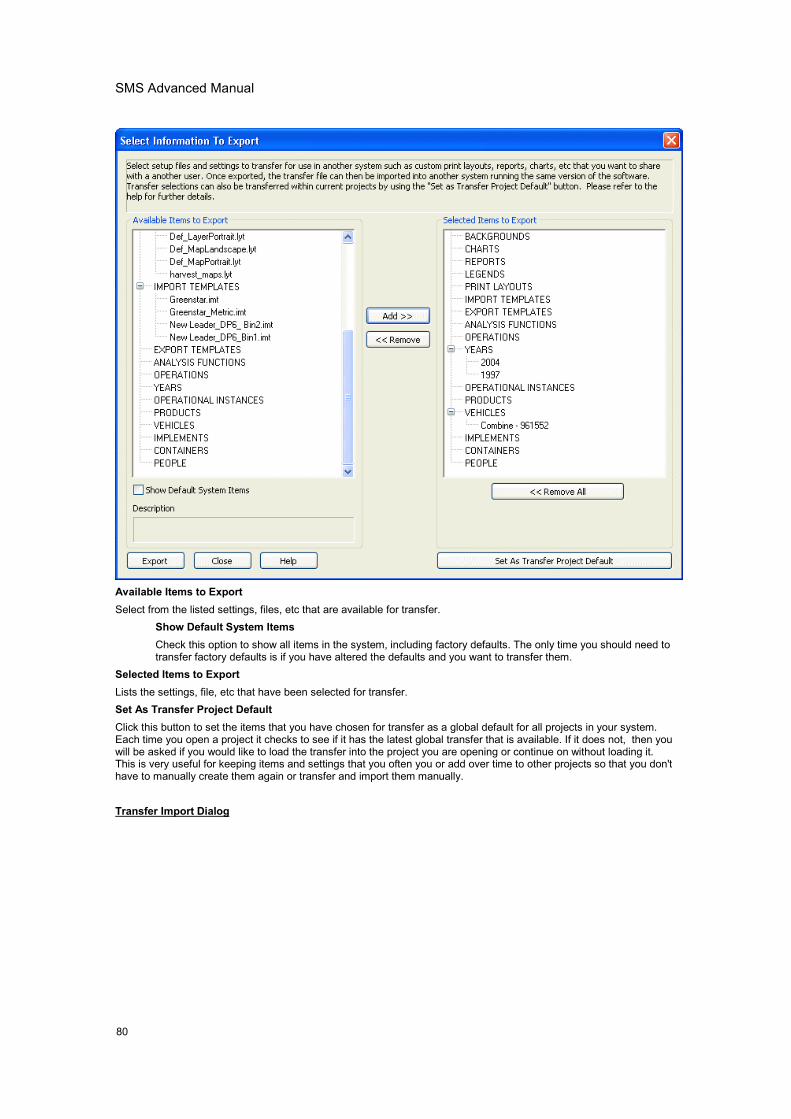
SMS Advanced Manual

80

Available Items to ExportSelect from the listed settings, files, etc that are available for transfer.

Show Default System ItemsCheck this option to show all items in the system, including factory defaults. The only time you should need totransfer factory defaults is if you have altered the defaults and you want to transfer them.

Selected Items to ExportLists the settings, file, etc that have been selected for transfer.Set As Transfer Project DefaultClick this button to set the items that you have chosen for transfer as a global default for all projects in your system.Each time you open a project it checks to see if it has the latest global transfer that is available. If it does not, then youwill be asked if you would like to load the transfer into the project you are opening or continue on without loading it.This is very useful for keeping items and settings that you often you or add over time to other projects so that you don'thave to manually create them again or transfer and import them manually.

Transfer Import Dialog

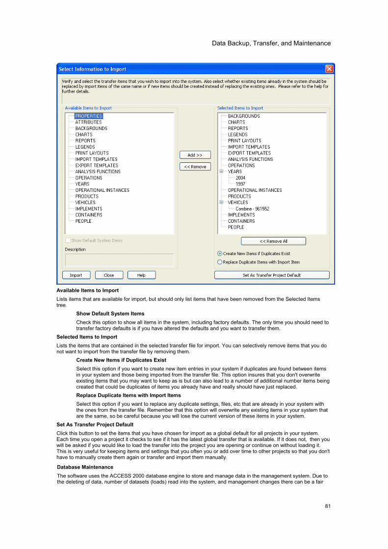
Data Backup, Transfer, and Maintenance

81

Available Items to ImportLists items that are available for import, but should only list items that have been removed from the Selected Itemstree.

Show Default System ItemsCheck this option to show all items in the system, including factory defaults. The only time you should need totransfer factory defaults is if you have altered the defaults and you want to transfer them.

Selected Items to ImportLists the items that are contained in the selected transfer file for import. You can selectively remove items that you donot want to import from the transfer file by removing them.

Create New Items if Duplicates ExistSelect this option if you want to create new item entries in your system if duplicates are found between itemsin your system and those being imported from the transfer file. This option insures that you don't overwriteexisting items that you may want to keep as is but can also lead to a number of additional number items beingcreated that could be duplicates of items you already have and really should have just replaced.Replace Duplicate Items with Import ItemsSelect this option if you want to replace any duplicate settings, files, etc that are already in your system withthe ones from the transfer file. Remember that this option will overwrite any existing items in your system thatare the same, so be careful because you will lose the current version of these items in your system.

Set As Transfer Project DefaultClick this button to set the items that you have chosen for import as a global default for all projects in your system.Each time you open a project it checks to see if it has the latest global transfer that is available. If it does not, then youwill be asked if you would like to load the transfer into the project you are opening or continue on without loading it.This is very useful for keeping items and settings that you often you or add over time to other projects so that you don'thave to manually create them again or transfer and import them manually.

Database MaintenanceThe software uses the ACCESS 2000 database engine to store and manage data in the management system. Due tothe deleting of data, number of datasets (loads) read into the system, and management changes there can be a fair

SMS Advanced Manual

82

amount of wasted or unused space in the database which can slow down the performance of the system. To keep thesystem performing at a high-level, it is recommended that you use the Compact Files� feature located under the Toolmenu. This function will cleanse your database of unused information that is wasting space. This feature will alsooptimize the database to increase performance. It would be good practice to run this feature once a month.

83

,��---�

How to read logged data files into the system.Follow these steps to read files into the system:

1. Start the program.2. Now select where you will be reading the file(s) from. If you want the program to auto-detect new files then

select File and then Open Card� or the Open Card icon on the Main toolbar. This will search your defaultsearch drive for new files in the selected file group. If you would like to specify a location to open a file from,select File and then Open� or the Open icon on the Main toolbar. The Select Files dialog will now appearfor either method that you choose.

3. Click Add Files to select a file(s) to be processed, if no files were detected or you selected the manualmethod of selecting files..

4. Once all the files to be processed are listed in the dialog, click Next>.5. If prompted, select an archive data type for the file. This will happen with all Harvest or Site Verification files

from Ag Leader�s YM2000�s and early firmware versions of the PF3000 as well as all Case IH AFS yieldmapping systems. Newer Ag Leader PF3000 YLD�s provide the information to auto-detect the type whenread in.

6. If the data is from a monitor that has not been read into the system before, select or create a Grower andFarm to associate the data in the file with and then click ACCEPT. Case IH�s and New Holland�s ENS fileformat contains a Farm name and only requires the creation/selection of a Grower for data from a newmonitor. Flexi-Coil�s LOG and the Ag Leader Insight ILF files contain a Grower and Farm name that willautomatically be filled in for data that is new to the system. If the file being read in is an Ag Leader BDY,TGT, or PFN file more management information will be required before clicking ACCEPT.

7. A dialog with the processing and management options is now displayed. Verify that all the managementoptions in the grids are correct and then, if desired, check the other settings by clicking on the available tabs.Click Next> to continue.

8. The file(s) will now be processed and entered. When processing is finished, the data is selectable in theManagement Tree.

How to migrate your data from Precision Map 2000 or Instant Yield Map SoftwareFollow these steps to transfer data from Precision Map 2000 or Instant Yield Map Software:

1. Start the software.2. Go to the File Menu and then select Open or select the Open icon from the main toolbar.3. The Select Files dialog will now appear on the screen. Click on the Add File(s) button.4. The Open dialog will now appear. Now click on the down arrow to the right of the Look In: box. Now select

the location where you installed Precision Map or Instant Yield Map and find the folder that contains theserial number of your monitor(s). This folder will contain all the YLD files that you have read into PrecisionMap 2000 or Instant Yield Map for that monitor. Select all the files that you would like to read in and thenclick the Open button.

5. You will now return to the Select Files dialog. The files to be loaded into the system will now be listed in thedialog. If all the selected files are from the same year, Grower, Farm, and are of the same Operation Typeand you would like to read the files in quicker, you can select the Batch Process Files item. If you are readyto continue and load these files, click the Next> button and follow the rest of the directions for reading filesinto the system.

Note:The same procedure as above should be used to transfer data from other mapping software programs that you havebeen using that kept an archived YLD file. Locate the YLD files within the program and follow the steps detailed above.

How to import Greenstar data.Greenstar data can be imported either directly from the GSY files that are logged or via an ASCII text file that can beexported from JDMap or JDOffice and then imported into the software using a template. Reading directly from theoriginal GSY files is recommended.

Follow these steps to import Greenstar data into the system:1. See How to read logged data files into the system.OR1. Go to the File menu and select Import, then Using a Template.

SMS Advanced Manual

84

2. The Select Template dialog will now appear. Click the Browse button for Template File and then select theGreenstar.imt file in the Open dialog and click Open.

3. Click the Browse button for Import File and select the Greenstar ASCII text data file that was exported fromyour software. Click Open.

4. Select a Data Type and a Management Type for the imported data. Select Grain Harvest for the Data Type ifthe data being imported in yield data. Select Add to Management Hierarchy for the management type. ClickNext> once you make these selections.

5. The attribute columns should all be set and ready to continue. Make sure that there is data for all thecolumns that are set and that they match properly. Click Next> when done.

6. Select the management information for the imported data then click Next>.7. Click Finish.

How to reprocess data.Follow these steps to reprocess load data that has already been read into the system:

1. Select the load(s) that you would like to reprocess from the Management Tree, either by selecting theOperation Instance to select all the loads below it or selecting an individual load(s).

2. Click the right mouse button and select Reprocess Data�from the menu that pops up.3. A dialog with a settings tab(s) will now appear, depending on what settings can be reprocessed for the

selected data. Make the settings changes that you would like applied to the selected data and then click OK.4. If more than one file contains data for the selected loads then the settings dialog will reappear for each file.

Repeat Step 3) for each of these dialogs.5. Once all the files have been set, the software will begin reprocessing the load data based on your edited

settings.6. Reselect the reprocessed data from the Management Tree to see the effects of the changes that were

made.

Note: Currently only YLD files support reprocessing of data. All other formats can only be reprocessed through theReprocess File(s) functionality.

How to set your map projection.Follow these steps to set the default map projection for all maps that made:

1. To create a more accurate map of your data you need to select a special projection that is specific to thearea you farm, click on a Grower in the Management Tree.

2. Click the right mouse button and select Edit Item.3. Click on the Projection Tab.4. Click the down arrow in the box under Datum and select NAD83 for example for the United States.5. Click the down arrow in the box under Projection and select the state and region description that best fits the

area you farm.6. Click OK. Any new maps you make will now reflect this change.

Note: Reference maps showing UTM zones for the entire world and State Plane regions for the United States areavailable by clicking the Help button on the Projection tab.

Using the Management TreeThe Management Tree allows you to quickly and easily find information that you would like to view.

The following steps describe how to use the Management Tree to find information that you are looking for:1. Click on a Grower name. A map of all the farm boundaries (If defined) and fields associated with the Farm

and Grower should appear in the Preview Window (if it is active). Summary information should also appearin the summary window showing all the Farms and Fields that are associated with the Grower. A map cannow be created/added to the Map Window as a boundary layer.

2. To proceed down in the tree, double-click the left mouse button on the Grower name. The tree will expand toshow all the Farms associated with the Grower. The Management Tree will automatically expand to the nextlevel that has multiple entries, so if all the following levels down to the Load level only have one entry thenthe tree will expand all the way down to that level. The Summary Window will now display a list of Fieldsassociated with the Farm and the Years that data is available. Click on a specific Farm to see a boundarymap of the Farm (if defined) and all the Fields associated with the Grower and Farm in the Preview Window,if it is active. Double-click on a Farm to expand it and see a list of the fields associated with it. A map cannow be created/added to the Map Window as a boundary layer.

3. Now double-click the left mouse button on a Farm and/or click on a Field. A boundary map for the fieldshould now be displayed in the Preview Window (if there is spatial data for that field). The Summary Window

How to ...

85

should now display the Years and Operation Types that data is available for the selected field. A map cannow be created/added to the Map Window as a boundary layer.

4. Next, double-click the left mouse button on a Field name and/or click on a Year. The tree will now expand toshow a list of all the Years that data is available for the field, or expand to the next level with multiple entries.The same boundary map as above should still be visible in the Preview Window (if active). The SummaryWindow will now display the Operation Types that data has been collected for in that Year and theCrop/Products that were used. A map can now be created/added to the Map Window as a boundary layer.

5. Now double-click the left mouse button on a Year and/or click on an Operation Type. The tree will nowexpand to show a list of all the Operation Types that data is available for that Year or expand to the nextlevel with multiple entries. The same boundary map as above should still be visible in the Preview Window (ifactive). The Summary Window will now display the Crops/Products and the Operational Instances that datais available for. A map can now be created/added to the Map Window as a boundary layer.

6. Next, double-click the left mouse button on the Operation Type and/or click on a Crop/Product. The tree willnow expand to show a list of all the Crops/Products that data is available for or expand to the next level withmultiple entries. A default data map should now be displayed if spatial data is available in the PreviewWindow, if active. The Summary Window should now display field summary information for the selection ifavailable. A data map can now be created/added to the Map Window.

7. Now double-click the left mouse button on the Crop/Product and/or click on an Operational Instance. Adefault data map should now be displayed if spatial data is available in the Preview Window (if active). TheSummary Window will now display load summary information for all the loads that data is available for. Adata map can now be created/added to the Map Window.

8. Lastly, double click the left mouse button on the Operational Instance and/or click on a Load. A default datamap should now be displayed for the selected Load in the Preview Window, if active. The Summary Windowwill display the summary information for the selected load. A data map of the selected load can now becreated/added to the Map Window. You have now reached the bottom level of the Management Treehierarchy.

Note: All levels in the Management Tree that have a (+) or (-) next to then can be expanded or compressed. Double-click on the item with the left mouse button to do this.

Using the Preview WindowThe following steps outline a general procedure for using the Preview Window:

1. Start the software.2. Make a selection(s) in the Management Tree.3. If the Preview Window is not visible by default, it is located below the Management Tree, then select View

from the main menu then click Preview Window. The Preview Window should now be displayed.4. If spatial data is available for the selection(s), then a map of the data should be visible in the Preview

Window. The map that is displayed will depend on the level at which you have made your selection in theManagement Tree. If you selected any level above Crop/Product then you will see a boundary map for theselection(s), if you have selected the Crop/Product level or a lower level then you will see a default data mapfor the selection(s).

5. If you would like to create or add to a map then click on the appropriate button at the top of the PreviewWindow or click on the appropriate icon in the main toolbar.

Note: The Preview Window can not be zoomed, unless you have a wheel-type mouse, or edited. It can however beundocked from its default location, resized, or turned off.

Using the Calendar View.Follow these steps to use the Calendar View:

1. Click the Calendar View Tab in the Main Window. The Tab should switch and you will now see a calendardisplayed where the Management Tree was previously.

2. The area above the calendar displays the available tools for working with the calendar. The current dateshould be displayed in a selection in the upper right corner of the window.

3. Adjust the date to a time when you know you have logged data, such as the month and year that you haveharvested with a yield monitor and GPS receiver. The date can be changed by selecting the number youwant to edit and either typing in a number or using the arrow keys on the keyboard to increment the values.Additionally, you can select the down arrow beside the date values and a small calendar will appear that youcan use to select a new date.

4. Once you find a date range with spatial data in it, you will see a gray bar(s) with a Year/Product/Operationbased name. These bars are called Calendar Events and are based on a grouping filter that can be set togroup data into events of your choosing.

SMS Advanced Manual

86

5. Left click on one of the gray boxes; it should then turn blue to indicate it is selected. The Summary Windowshould now update with a summary of the selected calendar event. This summary view is different thanother summaries in that it lists different management items together and provides a sum of the entries at thebottom. The summary can also be printed.

6. In addition to the Summary, displaying the Preview Map should display all the data for the selected calendarevent, which can then be mapped. This is an excellent way to make a quick map of all your Soybean or Cornharvest data, for example, with one button press.

7. You can also change the resolution of the calendar between a Month, Week, and Day View for betterresolution of the calendar view. On the Day View, Daily Stats/Info is also available that summarizes the datathat was collected on that day, but no map will be displayed.

8. Two filter and grouping buttons are available above the calendar view:

�� The first filter is a standard Data Filter that limits the data that can be viewed in the calendar, suchas only displaying data from a certain Grower or an Operation.

�� The second button is for selecting the calendar event grouping. This allows you to organize howthe calendar will group the data it displays. For example, you could set the grouping to displayevents by Operator, Field, and Product or Vehicle, Field, and Operation. You are only limited bythe management items that are in the system and the properties associated with thosemanagement items.

9. A print button is also provided in the Calendar View that will print the current calendar that is displayed, andin the format that it is displayed.

10. Notes can also be added to a date on the calendar by selecting a day in the calendar, which should thenhighlight at the top in blue, click the right mouse button, and select the Add Event... function. This will allowyou to add text notes that will only be available in the calendar, but provides yet another way for you todocument your operational activities.

11. Lastly, you can select to view more detailed information on a calendar event by double-clicking with the leftmouse button on a calendar event bar or by clicking your right mouse button with a bar selected andselecting View/Edit Event... from the menu that appears. This will bring up the View Event dialog which willdisplay a tree of all the management items and datasets that make up the selected event. Mostmanagement items can even be edited from this view, except for Farm and Field.

How to make a mapFollow these steps to create a map:

1. Start the program.2. Select an item from the Management Tree that you would like to make a map of. Items in the tree displayed

in a bold font contain GPS/spatial data that can be mapped.3. If the Preview Window is open, then a map of the selected item should be displayed in the window.4. Click on the Create New Map Button or Icon.5. A new map containing the data shown in the Preview window, and selected in the management tree, will

now be created and shown in the Map window.

How to Add a Layer to a Map.Follow these steps to add a data layer to the current map:

1. Select and map data from the Management Tree.2. Now select another dataset or use the same one that was used to create the map in the previous step from

the Management Tree.3. Click the Add to Current Map>> button above the Preview Window or go to the Map menu and select Add

Selection to Map.4. The new layer was added to the Layer Window as the top layer. It will be represented as a button with a "1"

next to the name and the button will have a red outline around it indicating that it is the current layer. Thefirst layer that was used to create the map will now be located at the bottom of the Layer Window and have a"2" labeled on the button next to the name.

5. You now have two layers in the map. Click on the layer button for a layer in the Layer Window to switch tothat layer and display its options and legend. Right-click on a layer button to see other options for the layeror layers such as rename, change position, and remove layer.

Or1. If you would like to make a copy of a layer that is already open in the active map, click your right mouse

button over the layer button for the layer to be copied or click the Layer Display Options button on the activelayer display.

2. From the menu that appears select Copy Layer and Add to Map.3. A copy of the layer will now be added to the Layer Window.

How to ...

87

Note: For best results when working with layers, set overlaying layers so that they can be identified from the otherlayers. Do this by setting colors, map type, and transparency different for each layer so that you can tell layers apart. Ifthis is not possible then the multi-layer query feature can provide meaningful numerical information when visually youcan not tell the layers apart.

How to display the 3D Terrain View.Follow these steps to display the 3D Terrain View:

1. Create a new map from a selection in the management tree.2. Now select the Hide/Show 3D View button on the Map Toolbar or select Map from the main menu and then

Hide/Show 3D View.3. Your map should now switch into 3D Terrain View. Various tools are provided for the manipulation of the 3D

view such as the Rotate and Reset Map Rotation options in addition to the fact that all the zoom and pantools are also still functional.

4. You can toggle back and forth between the 3D and 3D views by selecting the Hide/Show 3D View option.5. The 3D Terrain View can be printed or saved as an image just like a normal 2D map.

NOTES: Tooltips do still work in 3D Terrain View, but depending on the rotation you may see some offset inwhere the you think your cursor is located on the 3D view and what tooltip value appears. This is due to theviewing angle you have the map rotated to. Also, query does not work when in 3D Terrain view.TIPS: If your 3D terrain View doesn't look realistic, has obvious errors in it, or doesn't show enough variation(your ground is fairly flat) there are options for improving the display in 3D.

�� The 3D grid surface that is used to display the 3D Terrain View is built by default as an average ofall the data that you read into the system that contains the required attributes for building a 3D grid.Any data read from an Ag Leader, Case IH, or New Holland monitor will meet these criteria. If youhave access to higher accuracy position data, like from an autosteer system, you can importposition and elevation data from to generate a new 3D grid surface using the Regenerate 3D Grid.The Regenerate 3D Grid Batch Command, which may actually be easier for selecting multipledatasets. Once you have regenerated the 3D Grid, remap the data in question and view it in 3D tosee if the terrain view is improved.

�� If for some reason you can fix the problem by filtering out a few datasets from the 3D grid, you canapply a more permanent filter to your data. Add a Simple Analysis Filter to your dataset(s) thatcontain bad elevation data. Add this filter for the Elevation attribute and make sure to set the MINand MAX values for the filter to ones that best fit the real range of your data, like 800 to 1000 ft.Once you have filtered your data use the Regenerate 3D Grid feature (either on management treeselections or via batch command) and remake your map and check the 3D Terrain View.

�� If you can't get acceptable results with of these options or you would prefer more accurate data thenyou can import a DEM (Digital Elevation Model) and set this imported data as the 3D Grid. Importyour DEM data into the Management Tree. Then select the DEM dataset in the tree, click the rightmouse button and then select Set 3D Grid. Remake your map and you should now see a newterrain view that uses the DEM dataset for the 3D grid surface. (DEM's are not useful for mappingand are only intended for import and setting a 3D grid and not anything else.)

�� Lastly, if your terrain is fairly flat (lets say around 10 ft or less of elevation change across your field)the 3D Terrain View by default will provide little use because your map will appear relatively flat. Butthere is a display option that you can set to magnify elevation changes across your field so that youcan see a more useful 3D Terrain View. Just because you don't have hilly or sloping group does notmean that small elevation changes across your field aren't causing crop production issues. To scaleyour elevation data, with your data mapped, click on the Edit Map Options button on the MapToolbar or go to the Edit Menu and select Map Options. Then click on the 3D Map tab and enter avalue for the Elevation (Z-Axis) Scale Factor. A scale factor from 0.1 to 20 can be entered but wewould recommend that you start with a value of between 2-4 to test the result you get. This scalefactor can also be set as a default for all new maps by setting this same setting under GeneralOptions and 3D Map.

Using the Layer WindowThe Layer Window provides you with direct control of how data is organized and viewed in a map.

The following steps show how to use the Layer Window:1. Start the software. Select an item(s) with spatial data (any item whose name is displayed in bold text) from

the Management Tree. Create a map.

SMS Advanced Manual

88

2. The Layer Window should now appear to the right of the Map Window. A button outlined in red should belocated at the top of the window with a "1" on the left side of the button followed by a name based on thelevel at which the selected data came from in the Management Tree.

3. You can now select from the available settings and properties for the type of data layer that you created.This could include the map type such as circle or contour map, what attribute to display, transparency levelfor the layer, change the map properties, edit the legend for the current attribute, etc.

4. You can also place your mouse cursor over the layer button and click the right mouse button to see a menuof options for displaying the layer. These include the position of the layer in terms of others layers, editingthe layer name, creating a copy of the current layer, and removing the layer from the map.

5. Now you can adjust the size of the Layer window by placing you mouse cursor over the left or right edge ofthe Layer window until you see your cursor change to lines with arrows on each side. Now press and holdyour left mouse button and drag the window to the size that you would like.

6. Lastly, you can undock the Layer window from its current position and re-dock it next to the ManagementTree window or let it float as its own window. To do this, place your cursor over the two horizontal bars at thetop of the Layer window. Now press and hold your left mouse button and start dragging the Layer window tothe location where you would like to place it. The Layer window will only dock with the left or right side of theMap window, so if you want to re-dock it drag the window towards one of these sides until your mousecursor touches or crosses one of the sides. The Layer window should automatically snap into place and re-dock with the Map window. You can also double click on the title bar of the Layer Window when it isundocked to re-dock it in its default location.

How to adjust layer and attribute/property options.Follow these steps to adjust layer and attribute/property options:

1. Create a map or add a layer to a map of a selected management item.2. Go to the Edit Menu and select Layer Options or click on the Edit Options button in the Layer Window.3. The Layer and Attribute/Property Options dialog will now appear. This dialog allows you to set options for the

current Layer, Sub-Layers, and the current attribute or property.4. You now have the following options that can be set:

�� Layer - Tooltips that will be displayed for each map display type, the results that will be displayedfor queries for each map type, and the labels that will be displayed and their placement.

�� Sub-Layers - Visibility for Marks, Notes and attributes to be displayed for each, tooltips to bedisplayed, results to be displayed for queries, and labels to display and their placement.

�� Attribute/Property - Legend and map display type settings, drawing and display options fordatasets, and grid, contour, clipping settings (Only for attributes).

5. Once you have made the desired option settings, you can save your settings to apply to other datasets oronly when the current dataset is mapped. The following save options are available:

�� Layer Settings - Save all Layer and Attribute/Property settings for the current dataset only or for alldatasets of the same operation type, such as Grain Harvest.

�� Sub-Layer Settings - Save the Sub-Layer settings for the current dataset only or for all datasets ofthe same operation type.

�� Spatial Attribute/Property Settings - Either save the Attribute/Property settings only for currentdataset, all datasets of the same operation type, or save both the Layer and Attribute Settings atthe same time.

Example: If you had a field that you were doing variety comparisons in and you wanted to add a tooltip thatdisplayed a property you had created for Variety, but you only wanted it to display when you were mapping thisparticular field. To do this you would add the Variety property to the list of tooltip attributes/properties to bedisplayed, click the Save Layer Settings button on the Layer tab, and select Data Selection Default. Now the addedtooltip property will only display when you map the current dataset. If you wanted all the other datasets of the sameoperation, Grain Harvest, to get the same tooltip when mapped then you should select Data Type Default as yoursave option.12. Once you have made your all your desired options settings and saves, click the OK or Apply button to

regenerate the current layer in the map with your settings.

How to edit point data.Follow these steps to edit point data in the system:

1. Select an item from the Management Tree and create a map or add to an existing map. Only a Point(Spatial) type can be edited, so make sure the data display is set to one of these types.

2. From the Map menu, click Edit Layer� or click on the Edit Layer icon on the Map Toolbar. Note: Only pointdata for the current layer can be edited.

3. The Point Data Edit window will now appear. Use the selection tools in the toolbar to select the points to edit.

How to ...

89

4. You now have the option to either Move the point(s), delete the point(s), or straighten the selected points.5. To Move selected points click on the Move Item icon. You can then drag the point(s) to the new desired

location.6. To delete selected points click on the Delete Item icon. The points will be removed from the display. Note: If

a whole load is selected to be deleted in your selection area, all the points in the load will not be deleted.This is because of load references in the map. To delete a whole load select the load in the ManagementTree, click the right mouse button, and select Delete Branch.

7. Click on the Save button to save the modified dataset to the database.

How to straighten a pass on a point dataset.Follow these steps to manually straighten GPS point data in a pass:

1. Select and map a dataset(s) that you would like to straighten GPS points for.2. Go to the Edit menu and select Layer or click on the Edit Layer icon on the map toolbar.3. The Point Map Editor will now appear.4. Now select the points or pass that you would like to straighten using the selection tools.5. Once you have made your selection(s), got to the Edit menu on the editor and select Straighten Pass or click

on the Straighten Pass icon on the editor toolbar.6. Now draw a line or line segments that represent the new path that the points that are selected should be

placed in. Once you have drawn the new path, click the right mouse button to display the straightened datapoints.

7. The Straighten Pass tool can continue to be used as along as the points are selected so that you can get thepoints straightened exactly as you desire.

8. Once you have made the desired changes click the SAVE button to save the new point position.

How to edit a legend.Follow these steps to edit a legend in the system:

1. Select and map data from the Management Tree.2. Go to the Map menu and select Edit Legend or click on the Edit Legend button in the upper right hand

corner above the Legend Window in the Layer Window.3. The Edit Legend dialog will now appear. Select the options that you would like to change and make your

changes. To edit range values click on the cell that contains the range to be edited and type in the newvalue. The software will provide feedback if the entered value is not valid. To change the color for a range,double-click on the color you want to change and the Color Selection dialog will appear. Make your selectionand click OK.

4. Once you have made the desired changes to the legend, you can either apply the change or save the editedlegend and set it as a default. If you would like to save the legend, click the Save button, enter a name forthe legend or select a legend from the list to replace and then click the OK button. If you would also like tosave the legend as a default make your selection in the Default Selections area before clicking OK.

5. Now click the OK button on the Edit Legend dialog to return to the main map and view the edited legend.

How to freeze a boundary.Follow these steps to set a boundary for the Spatial Sorter and also to prevent the adding of more area to theboundary:

1. Select a Field from the Management Tree that you would like to freeze the boundary for. You can also selectat the Grower and Farm levels to freeze all the Field Boundaries below the selection. Batch Freezing ofmultiple Growers and Farms can also be done through the Batch Command Utility.

2. The boundary area map should appear in the preview window. If the boundary is representative of the actualfield area and is complete, click the right mouse button with your cursor positioned inside the ManagementTree Window. Select Freeze Boundary.

3. The boundary in the Preview Window should be replaced with a new boundary that has a black borderaround its edges and also around internal regions that show up as holes. This boundary can now be editedby creating a map of it and selecting Edit Layer from the Map menu or the Edit Layer icon from the MapWindow Toolbar.

Note: The frozen boundary will not automatically update if new data from that field is read into the system. If this is thecase or you would like to return to the automatic boundary then select the Field and then the Crop/Product level thatyou would like to base the auto boundary off of, click the right mouse button and select Regenerate Boundary. Theboundary will now be based off the selected dataset, and will update if new position information for this field, that iscurrently not covered, is read in. Doing this also removes this Field from those that will be spatial sorted, so usecaution when doing this if you have used the Spatial Sorter in the past on the selected field.

How to create a new attribute.

SMS Advanced Manual

90

Follow these steps to create a new attribute:1. Go to the Tools Menu and select Attribute Editor.2. The Select Attribute dialog will now open.3. Click the Add New button to create a new user-defined attribute.4. The Attribute Editor dialog will now open.5. Enter a name to be used to identify the attribute, such as Soil Compaction if you had data from a soil

compaction sensor to import.6. Now select a Data Type from the available list of options. For a description of the various data type options

for an attribute go to the help for the Attribute Editor.7. Depending on the Data Type that was set you will be required to either set a Display Type, Dimension and

Display Units, or none of these in the case of a Text data type.8. Now set whether or not the new attribute should be mappable. Check the mappable box to make the new

attribute available to map from the Layer Window when you map a dataset or management item thatcontains the attribute.

9. Lastly, set whether or not you want totals to be displayed in summaries,etc for the attribute and if so whatunits the totals should be displayed in. So your logged values for each point can be shown in one unit andthe totals amounts of all the values can be shown in another more appropriate unit.

10. Click OK once all the settings have been made above to create the new attribute.11. Click the Close button to exit the Select Attribute dialog.

How to create a new property.Follow these steps to create a new property:

1. Go to the Tools Menu and select Property Editor.2. The Select User Property dialog will now open.3. Click the Add New button to create a new user-defined property.4. The Property editor dialog will now open.5. Enter a name to be used to identify the property, such as Hybrid if you would like to enter property values for

a crop hybrid.6. Now select a Data Type from the available list of options. For a description of the various data type options

for a property go to the help for the Property Editor.7. Depending on the Data Type that was set you will be required to either set a Display Type, Dimension and

Display Units, or none of these in the case of a String data type.8. The last setting is whether or not the new property should be mappable. Check the mappable box to make

the new property available to map from the Layer Window when you map a dataset or management itemthat contains the property.

9. Click OK once all the settings have been made above to create the new property.10. Click the Close button to exit the Select User Property dialog.

Note: Properties can be added in bulk to multiple management items or datasets using the Batch Command Utility.

How to create/edit a custom Operation.Follow these steps to create/edit a custom Operation:

1. Go the Tools Menu and select Management List Editor.2. The Edit Management List Editor will now appear. Select Operation from the list and then click the Edit

List... button.3. The Edit Item dialog will now appear. Click the Add New button.4. The Edit Operation dialog will now appear. Enter a name for the operation on the Operation Info tab. Choose

a name that clearly identifies your new operation, such as Weather Conditions for example.5. Now click on the Operation Definition tab. Select an Attribute Group and then an attribute from that group

and add it to the list of selected items for your new operation. Check the Required for Import option for theselected attribute if you want to require that the attribute be assigned to one of the import attributes whenimporting data. Repeat this step for each attribute that you want assigned to this new operation. Click OKwhen you are done.

6. The Operation you created will now be available to select when saving data created in editors, as one of thedefault Operations that you can select when creating a new Generic dataset, or when importing data.

How to ...

91

Note: The Operation you created can also be adjusted from the Edit Item selection, available in theManagement Tree when you have an custom operation selected.

How to define ProductsFollow these steps to fully define a Product:

1. Select a product in the management tree that you would like to set or edit the properties for.2. Click your right mouse button. The Management Tree menu should appear. Select Edit Item. The Edit

Product dialog will now appear.3. The following tabs should have values set for the properties they contain, depending on the intended usage

and tracking of the product:

�� Product InfoThis tab contains general information to define the type of product being used. Enter a custom ProductName that best describes the actual product, such as the Hybrid or variety name for a seed product.Then set a Product Group such as Grain for a product that will be used for seed and then harvested, thiswill also try the available settings for the product on the Product Description tab. Now select a ProductUsage to further define how the product will actually be used in your operation(s), i.e. Seed/Commodityfor a product that will be planted and harvested. The Crop Type should now be set to identify the cropthat the product should be associated with, mainly for filtering purposes on reports, maps, etc, so for aproduct that has been named based on its variety I would select a Crop Type of Soybeans. The ProductMix option is only available for Product Groups that are Application Rate related such as Fertilizing orChemical. The Description allows you to document details about a particular product. Lastly, the Is Activeoption defines whether or not the product will be available for selection as a product in the SelectManagement dialog when new data is being archived or data is being reprocessed.

�� Product MixThis tab is only available when Product Mix is checked on the Product Info tab. A Product Mix must bebuilt from products that have already been created or already existed in the system; you can not add newproducts from this dialog. Also it is recommended that your mixes add up to 100%, if defining your mix bypercentages to ensure resulting calculation based on the percentage of each product in the mix add upto the totals and averages for the mix. Product Mixes can also be defined by a Formula instead of usingpercentages. Formula based mixes allow you to define a mix that contains a mixture of different productforms, such as a liquid mix that has both liquid and dry products mixed into it. Product Mixes can only bedefined for products that are assigned to the Fertilizer or Chemical groups, and is best used when youhave blended products that you would like to track by the individual components that make up the mixedproduct.

�� Product DescriptionThis tab provides specific properties than can be set that are appropriate to the Product Group that wasselected on the Product Info tab. Fill in as much information has you have or feel like, but it is highlyrecommended that any entry that is highlighted in yellow be filled in with an appropriate for the product.Properties highlighted in yellow are ones that can be used in other calculations.

�� Product ConversionThis tab allows the definition of conversion values for the product for application rate and harvestoperations. These conversions are used to calculate values such as Product Used/Needed, ProductRefills Required, and Product Unloads. The Use Multi-Use Conversion is only available for products setto a harvest related Product Group and allows the definition of Mass and Dimensionless application ratesto cover situations where you may row plant, drill, or air seed the same product in the same year but stillwant to track it under one product.

5. Once your product has been fully defined or edited, click the OK button. Remember that if you forget to set aproperty value that you meant to or realize later that you want to set a value for a property that can be usedin a calculation, you can always go back and edit a products property values and all the data linked to theproduct will update appropriately.

How to add a property to a management item or dataset.Follow these steps to add a property to a management item or dataset:

1. Select a Grower, Farm, Field, or Dataset (Load/Region) in the Management Tree to add a property to.Properties can not be added to a Year, Operation, Crop/Product, or Operational Instance.

2. Click your right mouse button to display the Management Tree Menu and select Edit Item.3. Click on the Additional Properties Tab.4. Now click on the Add Property button to add a property.5. Select a property from the list of available user-defined properties or create a new property to use.6. Click OK once a property has been selected to add to the current management item.7. The selected property will now be displayed in a grid on the Additional Properties tab.

SMS Advanced Manual

92

8. To edit the value for the property that has been added, click on the Value grid cell next to the name of theproperty and enter a value of make a selection from the available options.

9. Repeat steps 4 through 8 to add more properties if desired.10. Properties can also be removed from a management item by clicking the Remove Property button and then

selecting the property(s) to be removed.11. Click OK on the Additional Properties tab once you have finished adding a property(s).12. The property(s) that was added can now be viewed in the Summary by selecting the Summary Tab and then

the Property sub-tab. The property can also be mapped by creating a map and then selecting the SelectedProperty item from the list of attributes in the Layer Window, clicking the Edit Property button next to thisselection, and then selecting the management item that the property was added to and selecting it.Properties can also be added to the general summary, reports, charts, and map printouts.

Or1. Go to the Tools menu and select Batch Command Utility. The Batch Command Utility dialog will appear.2. Under the Select a Batch Command combo, select Add/Set Property Value. Then click OK.3. You will now be prompted to set the data filters to select the management items/datasets to apply the

selected property to. Once you have set the desired filters click Next>.4. The edit Data Filter Results dialog should now appear. You can remove items that you do not want the

property added to or continue on with all the items shown in the results by clicking Finish.5. Select a property from the list of available user-defined properties or create a new property to use.6. Click OK once a property has been selected to add to the current management item.7. The selected property will now be displayed in a grid on the Additional Properties tab.8. To edit the value for the property that has been added, click on the Value grid cell next to the name of the

property and enter a value of make a selection from the available options.9. Repeat steps 4 through 8 to add more properties if desired.10. Click OK on the Additional Properties tab once you have finished adding a property(s).11. The property(s) that was added can now be viewed in the Summary by selecting the Summary Tab and then

the Property sub-tab. The property can also be mapped by creating a map and then selecting the SelectedProperty item from the list of attributes in the Layer Window, clicking the Edit Property button next to thisselection, and then selecting the management item that the property was added to and selecting it.Properties can also be added to the general summary, reports, charts, and map printouts.

How to edit property data.Follow these steps to edit property data:

1. Select a management item in the Management Tree that a property has been added to.2. Click the right mouse button to open the Management Tree menu.3. Select the Edit Item selection.4. Now click on the Additional Properties tab.5. A listing of the properties that have been added to the management item should be displayed along with the

value that has been entered for each.6. Click on a value a value entry that you wish to edit the value for and enter or modify the value.7. If you wish to remove a property instead of just edit it value, click the Remove Property button and then

check the property(s) that you want removed from the current management item selection. Click OK toremove the selected properties.

8. Once all the desired edits have been made, click the OK button to close the Edit dialog.

How to enter Financial Tracking entries.Follow these steps to enter Financial Tracking entries:

1. Go to the Analysis Menu and select Financial Tracking Entries or click on the Financial Entires Tab andselect the Add Item button from the toolbar or click your right mouse button in the tree area and select AddItem.. The Select Expense/Income Type dialog should now appear.

2. You now need to select an Expense/Income Type. There are 6 Expense/Income Types provided for you toselect from; Commodity Sales, Field Level Expenses, Field Level Income, Misc. Income (Per Operation),Operational Expenses, and Product Purchases.

3. Assuming you are adding (or even editing) an entry, you will now see the Expense/Income Info dialog. Thisdialog allows you to enter a name, description, and define the shares for the expense/income entry.

�� The first thing to do is enter a specific name and description that will allow you to easily identify anexpense/income entry from other entries. This is less important if you are trying to track individual

How to ...

93

expense/income amounts but instead totaling everything before entry into the software, but if youwant to track each individual expense/income amount that goes into and comes out of youroperation then you need to have descriptive names and descriptions to help you quickly and easilyidentify them on the Financial Tracking dialog as well as the Financial Tracking Report.

�� The last thing to do is to add any expense/income shares that you might have. If you want to addshares, check the Share Expense/Income by Percentage box, and then click the Add button toadd People to share the expense/income with and to define the percentage share each willreceive. The overall share percentage must equal 100% between all people that will be sharingthe expense/income. The share values will appear on your Financial Tracking Report as separatedata columns that allow you to see individual and overall totals for each share holder as well asoverall totals.

Once you have set the required info for the expense/income click the NEXT> button.4. The Expense/Income dialog should now appear. This is the dialog where you actually enter in your

expense/income amounts and values as well as assign them to a management item(s) and in some cases atime span to apply over.

�� The first thing to do is set where you want the expense/income values to apply to. Depending onthe Expense/Income Type you have selected, the available management selections that can beset will vary. You need to select the item or items that the expense/income entry will apply to, forexample for a Commodity Sale you would select a particular Year, Grower, Farm, Field, andProduct to apply the sale amount to. In the case of a Product Purchase though, you might havebought and applied enough product to cover 3 years of application of that product, that being thecase you want that expense to apply over multiple years. So you would select Multiple for the Yearselection and select all the years that the expense should spread out over. Then you would pickthe other specific links such as a Grower, Farm, Field, and Product.

�� The Second step, which is only available for the Product Purchases Type, is to set a time spanover which the expense should be applied. This is very useful when multiple purchases of aproduct are needed within a year and different prices were paid for each purchase instance. Bysetting a date span of when the purchase amount should apply, the software will only apply theexpense to data that meets the management link selections you made and also falls within thedate span you have selected.

�� The last step is to actually enter your expense/income values. The number and type of entries willdepend on the Expense/Income Type that was selected. There are basically three types offormatting for the entry values:

�� White background - Generic entries that are not used in a calculation and are notrequired for entry, they can be left blank without an affect on other values.

�� Yellow background - This is a required entry that is more than likely used as an inputinto an equation for calculating one of the other values.

�� Gray background - This is a calculated entry that is more than likely used as an inputinto an equation for calculating one of the other values or is the result of an equation.

Fill in the amounts as required and then click the CALCULATE button. This will then apply what evercalculations or totaling that is set for the value entries, and fill in the cells with the appropriate values.

NOTE: If you do not want to use the calculated results, you can manually type in a Per UnitValue in the last entry for each type to set the value you desire. If you do this then the othervalues above are not useful and should not be filled in and the CALCULATE must not beselected, otherwise it will override your manual entry.

5. You have now made a Financial Tracking entry and can run a report, profit/loss analysis, etc. The entry willbe displayed in the Financial Entries tree and you can select an entry from the tree to view all the details ofthe entry in the Summary document on the Financial Entries tab.

Note: You can edit or delete your Financial Tracking entires from the Financial Tracking Tree by selecting an entry inthe tree and then selecting the Edit Item icon from the toolbar or clicking your right mouse button with and entryselected and then selecting either Edit or Delete Item from the menu that appears.

How to generate a Financial Tracking report.Follow these steps to generate a Financial Tracking report:

1. First, make sure that you have added some Financial Tracking entries so that you will actually get resultswhen you run the report.

2. If you have entries, go to the Analysis Menu and select Financial Tracking Report.3. The Profit/Loss Report Options dialog should now appear. You need to select a resolution of detail for the

report that will be generated. Four filter levels are provided:

�� Year - Displays your profit/loss data grouped by Year and no other management items.

SMS Advanced Manual

94

�� Grower - Displays your profit/loss data by Year and grouped by Grower and no other managementitems.

�� Farm - Displays your profit/loss data by Year/Grower and grouped by Farm and no othermanagement items.

�� Field - Displays your profit/loss data by Year/ Grower/Farm and grouped by Field and no othermanagement items.

Now select a Data Source for the total amounts used in the report from the following available options:

�� Monitor Summary - Uses only summary totals from the monitor only, and doesn't use any spatialdata. This is the default selection and should provide the best indicator of profit/loss totals.

�� Spatial Records - Uses only spatial data for generating summary totals. This report will matchProfit/Loss analysis results the closest, but may not indicate actual profit/loss as closely since itstotals are based on spatial data only.

�� Manual Entries - Uses manual total values that have been entered for each dataset. Most usefulwhen you know exact totals that you want used, which the monitor or spatial sources do not match.

Once you have selected your filter level and data source, you can now also select to Show Individual Sharesin Report. This option will break down your expense/income entries and the profit/loss values per share thathas been defined. This is the only location in the software where this share information is calculated andtotaled. Once you have made all your selections click the NEXT> button.

4. You will now see the Select Data Filters dialog which will allow you to select the data you want included inyour report, such as ALL fields, a few select fields, or a single field for example. Once you have selectedyour dataset filters, click the NEXT> button.

5. The Edit Data Filter Results dialog will now be displayed and provides a tree view of all the datasets that metyour filter selections on the previous dialog. You can remove any datasets that are listed that you do notwant to be included in the generation of your Financial Tracking Report. Click the FINISH button once youare satisfied with the datasets that will be used for the report.

6. An Analysis Report document will now be displayed in the main window. In some situations an AnalysisChart will also be generated. You can now edit the analysis report/chart display options, such as logos,column names, the attributes to display on the report, etc. by clicking your right mouse button on thereport/chart and selecting Edit Report/Chart Options or under the EDIT menu and OPTIONS.

7. Once you are satisfied with the Analysis Report/Chart you can select to print the document or Save toImage. You can also save to a workspace to see the results when you open the workspace again.

How to create a 3D Plot.Follow these steps to create a 3D Plot:

1. Select a dataset from the management tree, either at the Operational Instance level to select all the datasetsbelow it or select an individual load/region dataset.

2. Now go to the File Menu, select New, and then 3D Plot or from the main toolbar click the New 3D Plotbutton.

3. A 3D Plot Document should now be created that displays your plot, legend, and 3D Plot toolbar.4. You can now change various display options for the plot such as the legend, colors used, the display type

(either bar or surface plot), etc. You are also provided with tools to rotate, zoom, and pan the plot.5. You can also either print the 3D Plot and its legend by going to the File Menu and selecting Print or by clicking

the right mouse button while the cursor is over the plot and selecting Print. In addition, you can save the 3Dplot and legend to an image file by going to the File Menu and selecting Save to Image or by clicking the rightmouse button over the plot and selecting Save to Image.NOTE: 3D plots can also be added to print layouts for the dataset that is currently displayed in the layout.

How to create a boundary.Follow these steps to manually create a boundary dataset:

1. Create a new map or add a layer to a map that you intend to create a boundary for.2. From the File Menu, select New then Boundary Layer or click the New Boundary icon on the Map Toolbar.3. The Boundary Editor dialog will now appear with a copy of the layer(s) that was in the Map window.4. Use the tools in the toolbar to add points or polygons, merge selections, snap points, and delete selections

to obtain the desired boundary.5. Select one the following or a combination to save or set the boundary:

�� Click Save to enter the new data into the Management Tree and save the boundary into theManagement Tree. Note: If you want this boundary to be displayed when you select the field inthe Management Tree or be used for spatial sorting, and you don�t do the step below of setting the

How to ...

95

boundary, then you must select the Boundary dataset in the Management Tree, click the rightmouse button, then select Set as Field Boundary to activate this boundary. The boundary will nowbe used for spatial sorting and also to be displayed as the default boundary for the field.

�� Click Set Field/Farm Boundary buttons to set the boundary for a Field or Farm but not enter it intothe Management Tree. To use a Field or Farm boundary for spatial sorting this option should beused.

�� Click Export to create an ESRI Shape, MapInfo MID/MIF, ASCII text file, or a BDY file for use inthe Ag Leader PF3000 or PF3000 Pro. Note: Boundaries exported as Ag Leader BDY�s will onlycontain one boundary feature, so if you have created sub-boundaries then only one of theboundaries will be exported and you will not be able to choose which one.

6. If Save is selected, select the management information for the new data and then click Accept.

How to edit a boundary.Follow these steps to edit a boundary in the software:

1. Select a Field from the Management Tree and create a new map or add a layer to the current map.2. From the Edit menu, click Layer� or click on the Edit Layer icon on the Map Toolbar.3. Use the tools in the toolbar to make any changes or additions.4. Click Save.

How to create a crop plan.Follow these steps to create a crop plan dataset(s):

1. The first step is to make sure that you have boundaries frozen or set for all the fields that you wish to createcrop plans for.

2. From the File Menu, select New then Crop Plan(s).3. The Select Crop Plan Operation dialog will now appear. Select a Crop Plan operation from the list to create

your new Crop Plan dataset(s) based on or create a new crop plan operation to meet your planning needs.The default crop plan operation is geared towards planting/seeding planning so if you would like to planother crop operation such as spraying or fertilizing then you will want to create a custom crop plan operationfor this purpose.

4. Once you have selected your Crop Plan operation click OK.5. The Select Crop Plan Products dialog should now appear. Select the Products from the available list that

you would like to use in your Crop Plan. Click OK once you have selected your desired products.6. The Define Crop Plan dialog will now appear. Select one Product at a time from the Products you selected

for the Crop Plan. Then select the field(s) that you would like to assign the Product to for your Crop Plan byadding them to the selected list. Then for each Product that you assign fields to, you can also set defaultattribute values that will get created with the Crop Plan dataset. Click NEXT once you have assigned yourProduct(s) to a Field(s) and entered the default attribute values.

7. The Select Management dialog will now appear. You only will need to set the Year, Operation, andOperational Instance to save your Crop Plan dataset(s) to. Click FINISH once you have made yourselections.

8. Your Crop Plan dataset(s) has now been created. Go to the Management Tree and open a field that youcreated a Crop Plan dataset for and you should be able to map your Crop Plan.or to create a Crop Plan for a single field and edit it immediately...

1. Create a map of the Field Boundary from the Field that you want to create a Crop Plan for.2. Then from the File Menu and New or the map toolbar, select the Field Crop Plan Layer.3. The Select Crop Plan Operation dialog will now appear. Select a Crop Plan operation from the list to create

your new Crop Plan dataset based on or create a new crop plan operation to meet your planning needs. Thedefault crop plan operation is geared towards planting/seeding planning so if you would like to plan othercrop operation such as spraying or fertilizing then you will want to create a custom crop plan operation forthis purpose.

4. The Select Management dialog will now appear. You only will need to set the Year, Operation, OperationalInstance, and Product to save your Crop Plan dataset to. Click FINISH once you have made your selections.

5. The crop Plan editor dialog will now appear with your polygon shown that covers the same area as your fieldboundary. It will be set to the same Product that you chose on the Select Management Tree.

6. Use the provided tools to divide, delete, and/or modify the crop plan polygon region or create additionalpolygons to assign products to.

7. Once you have your crop plan regions defined, you can use the Product legend to assign Products to thepolygon regions. Click the Edit Legend button to select additional products to use in your crop plan. Onceyou select a Product from the legend, click the Fill Product Regions button in the toolbar or select it from the

SMS Advanced Manual

96

Map menu. Then click on each region on the map that you want to assign the selected Product from thelegend to. Repeat as needed to assign all the regions to a product.

8. Once you have defined your Crop Plan regions and assigned products to them, click the Save button toupdate your Crop Plan dataset.

How to edit a crop plan.Follow these steps to edit your crop plan:

1. Select and map your Crop Plan dataset from the Management Tree.2. From the Edit menu, click Layer� or click on the Edit Layer icon on the Map Toolbar.3. The Crop Plan editor dialog will now appear with your product region(s) displayed.4. Use the tools in the toolbar to make any changes or additions to the crop plan dataset. You can also add

additional Products to your legend to assign to your crop plan region(s).5. Click Save when done to accept your changes..

How to create a generic dataset.Follow these steps to create a generic dataset:

1. Create a new map or add a layer to a map that you intend to create generic objects off of.2. From the File Menu, select New then Generic Layer or click the New Generic icon on the Map Toolbar.3. The Generic Editor dialog will now appear with a copy of the layer(s) that was in the Map window.4. Use the provided creation tools to add polygons, points, lines, circles, etc to the new generic dataset. You

can also use the Copy From Layer tool to copy an object from one of the layers that are visible in thebackground.

5. Once you have drawn, copied, or modified your desired objects for the new generic dataset, click on theData Grid tab.

6. Now you can add an attribute(s) and then set values for each object that you have created or copied. If youcopied from another layer you had the option to copy its attributes, which will now be displayed if you choseto copy them and they to can be edited.

7. Once you have created the desired objects, setup attributes and added values for them, click the Savebutton and set the management information for the new generic dataset. Click Accept when finished.

8. The generic dataset that you created will now be mappable, have summary information, available forgenerating reports and running queries on.

How to use the Average Data by Polygon Tool.Follow these steps for using the average by polygon tool:

Note: This tool can only be run on datasets that are vector (polygon) based and this tool does not make a newdataset, just an average of a user selected attribute is being created and added to that dataset. An example ofthis would be averaging point data, i.e. yield data by polygon, i.e soil type data.

1. Create a new map and add a dataset(s) to the current map for all data desired to be used in the running ofthe average by polygon tool.

2. Enter the Generic Editor and select the Copy from Layer tool and run though it, selecting the vector/polygondataset, and then copy all the objects into a new layer.

3. After the new layer has been created it can be used in the average by polygon tool. Since you have alreadyadded all the other datasets into this map in step one you can now run the average by polygon tool. Click theAverage by Polygon button or select it from the Edit Menu.

4. You should now see the Average Data by Polygon Settings dialog. In this dialog you have to set the Layerand the Attribute from the layer that you want to include in the average by polygon function and in the end itwill be added to the dataset that you just created in step 3. After you select the layer and attribute, you canjust �Add� it to the Selected Attribute list on the right side of the dialog. Once you have the layer attributesadded to the list you can click OK and then the tool will run. Depending on the amount of data and thecomplexity of the vector data this could take some time, so please wait for the hourglass to go away toindicate that the process is complete.

Note: You have the ability to create a new attribute in this dialog and remap the attribute that isselected to a new one. A example of this would be if you want to add multiple years of yield dataaverages by polygon. You can create a new attribute for each year of avg yield and just remap �Est.Volume (Dry)� to �Yield Dry 1998� and etc. In the end you would have multiple years of yield historyin the same dataset. The key is making sure to name each attribute variation to be output with a goodunique name that properly identifies it.

5. After the process is complete, if you view the Data Grid tab you will see the objects for the polygon layer andthe attribute information that was copied into the new layer and averaged by polygon.

How to ...

97

6. Once you are satisfied with the results you can save the new dataset into the management tree and use thedataset for other functions such as prescriptions, analysis, reporting, etc.

How to use the Vector Overlay Tool.Follow these steps for using the vector overlay tool:

Note: This tool can only be run on datasets that are vector based, i.e. if you want to merge two polygondatasets into one combined result by creating a whole new dataset. I

1. Create a new map and add any datasets to the current map that are intended to be used in the overlay andgenerated into a single new dataset. Multiple datasets can be used if desired to make a new dataset.

2. After the datasets are mapped, enter the Generic Editor and click the Vector Overlay tool button or select itfrom the Edit Menu.

3. You will now see the Vector Overlay Settings dialog. In this dialog you don�t have many choices. All youhave to choose is the datasets that you want to include in the overlay/merge process and then select if youwant the attributes from the datasets to be copied into the new overlay/merged dataset and then click OK.

4. After the process is complete you should see a new dataset that was created that includes the two datasets,combined into one. In every spot the two datasets intersected a new object/polygon was created and ifattributes where selected to copy then the attributes from the two layers are copied into the newobject/polygon. If you view the Data Grid tab you will see the objects and the attribute information that wascopied into the new dataset.

5. Once you are satisfied with the results you can save the new dataset into the management tree and use thedataset for other functions in the software such a prescriptions, reports, analysis, etc.

How to edit generic data.Follow these steps to edit a generic dataset:

1. Select a generic dataset from the Management Tree and create a new map or add a layer to the currentmap.

2. From the Edit menu, click Layer� or click on the Edit Layer icon on the Map Toolbar.3. Use the tools in the toolbar to make any changes or additions to the generic dataset or edit the values for the

objects on the Data Grid tab.4. Click the Save button to save any modifications to the original dataset or go to the File menu and select

Save As to save the changes to the generic dataset to a new dataset in the management tree.

How to create a guidance dataset.Follow these steps to create a guidance dataset:

1. Create a new map or add a layer to a map that you intend to create guidance data off of.2. From the File Menu, select New then Guidance Layer or click the New Guidance Layer icon on the Map

Toolbar.3. The Guidance Editor dialog will now appear with a copy of the layer(s) that was in the Map window.4. Two tools are provided for creating guidance data. The Copy Guidance Region tool should be used when

you enter the editor with a polygon type layer (like a field boundary) that you want to copy and use as theregion you want guidance in. The Draw Guidance Region tool should be used when you want to manuallydraw a polygon region that you want guidance generated inside of.

5. If you select...

�� Copy Guidance Regioni. Select a layer to base your guidance dataset of off and click NEXT>.ii. Now select the polygon objects that you would like to base your guidance dataset on.

Use the provided selection tools to make the desired polygon object(s) selection. ClickFINISH> once you have made your selection(s).

�� Draw Guidance Regioni. Draw a polygon region on the map that you would like to create a guidance dataset

from. Click the left mouse button to define the sides of the polygon area.ii. Click the right mouse button when you are finished defining the guidance region.

6. The Guidance Settings dialog will now appear. Enter a swath width to define the distance between yourguidance passes inside of the guidance area selected in the previous step. Click NEXT> button once youhave made your entry.

7. The Headland Settings dialog will now appear. Select the Headland Type and then based on the selectedtype set the available options for that pattern. If No Headland is selected then your guidance passes will begenerated to the edge of the guidance region that was selected or drawn. Click the NEXT> button whendone.

SMS Advanced Manual

98

8. The Straight Line Settings dialog will now appear. Set the available settings for generating the guidancepasses in the guidance region. Click the FINISH button when you are done to generate your guidancepasses.

9. The steps above can be repeated now if you would like to define additional guidance regions within thesame field and dataset. This might be useful if you have a field with areas that require a different pattern orheadlands to provide the best possible guidance.

10. Once you have created the desired guidance regions, click the Save button and set the managementinformation for the new guidance dataset. Click Accept when finished.

11. The guidance dataset that you created will now be mappable and even can provide resource trackingattribute results or be used in the Dataset Playback tool (Advanced only).Note: Your guidance dataset can be edited, but only the Guidance/Headland/Straight Line Settings can beedited. The guidance region that was defined can not be edited. If the region needs to be edited you mustrecreate it.

How to create navigation points.Follow these steps to create navigation points in the software:

1. Create a new map or add a layer to a map that you intend to create navigation points off of.2. Select a map type (Circle, contour, etc.) for the layer(s) that are on the map. Selecting the proper map type

for your layers can help in picking points to place navigation points.3. From the File Menu, select New then Navigation Layer or click the New Navigation icon on the Map Toolbar.4. The Navigation Edit window now appears with a copy of the layer(s) that were in the Map window.5. Use the tools in the toolbar to add, move, and delete points.6. Click on the Grid tab to view points that have been added and to manually enter point locations or edit the

name for a point.7. Click Save to enter the new data into the Management Tree or click Export to create a PFN file for use in the

Ag Leader PF3000/PF3000 Pro or an ASCII text file of the navigation points.8. If Save is selected, select the management information for the new data and then click Accept.

How to edit navigation points.Follow these steps to edit navigation points in the software:

1. Select a navigation dataset from the Management Tree and create or add to a map.2. From the Map menu, click Edit Layer� or click on the Edit Layer icon on the Map Toolbar.3. Use the tools in the toolbar to make any changes or additions.4. Click Save.

How to create a variable rate prescription.Follow these steps to create a variable rate prescription dataset:

1. Create a new map or add a layer to a map that you intend to use as a reference for the new prescriptiondataset.

2. Set the map type (Circle, contour, etc.) for the layer(s) that are on the map to a type that can be easily usedas a reference for the new prescription date set. For example if a layer is selected and gridded then theresulting prescription may have holes where there are larger gaps between points than the grid cell size thatis used. But if the layer was set to a contour type, the data would be smoothed over and when it wasconverted to a prescription dataset it would more closely resemble the reference layer in terms of theregions represented by the contours. Point and line layers in their base form can not be used as referencesfor a prescription, they muct first be gridded or contoured.

3. Once the reference layer to be used for the prescription has been added to the map and the map displaytype set, go to the File menu and select New and then Prescription Layer or select the New Prescription iconfrom the Map Toolbar.

4. The Prescription Reference Layer Selection dialog should now appear. Now select a reference layer fromthe list of layers that were open in the current map. Once a layer is selected it will display in the referencelayer preview window below. If None is selected as the reference layer, then a layer from the current mapwill not be used as a reference to automatically generate a prescription dataset. Instead the layers that wereopen in the current map will be used as a background for the Prescription Editor and the prescription datasetmust be manually "painted" in using the prescription editing tools.

5. Click Next> after the reference layer has been selected.6. The Prescription Attribute Type and Units Selection will now appear. Select an Operation type that the new

prescription dataset will be created as, i.e. a Planter Prescription. Now select a rate attribute type for theprescription data, i.e. Target rate (Seeds). Finally, select rate units for the selected rate attribute, i.e. sds/ac.

7. Click Next> once all the required information has been set for the new prescription dataset.

How to ...

99

8. The Edit Prescription Legend dialog will now appear. Select the number of ranges equal to the number ofunique application rates that are desired for the prescription dataset or load an existing legend that has beenpreviously saved. Enter individual values for each range. The range values will be automatically sorted asvalues are entered, from high to low at the bottom. Once the prescription legend is setup it can be saved forlatter use by clicking the Save button.

9. Click the Next> button once the prescription legend is complete.10. The Assign Legend Ranges dialog will now appear. Click on one of the ranges under Prescription Legend

Values and it will highlight. Now click on one or more ranges under Reference Layer Values and Map andthe selections will all highlight. Click on a highlighted item again to unselect it. Click the Add>> button toassign the selected Reference Layer value(s) to the Prescription Legend value that was selected. Thisassignment of values is displayed under Legend Assignment View. Repeat the steps above until all thereference layer values have been assigned to values from the prescription legend, unless it is desired thatnot all the reference values will be assigned rates. If you would like to remove or change an assignment,select the Reference Layer value to be removed or changed from the tree under Legend Assignment Viewand then click the <<Remove button. The Reference value(s) that were selected will now re-appear underReference Layer Values and Map. To remove all assignments click the <<Remove All button.

Hint: The reference layer map that is displayed below the range values for the reference layer can also be usedto make selections. Move your cursor over a region that corresponds to a legend range in the window above andclick the left mouse button. The range value that was selected on the map should highlight and can then beassigned by clicking the Add>> button.11. Click the Finish button after all the desired assignments have been made.12. The Prescription Editor dialog will now appear. The new prescription dataset will be displayed in it and the

Prescription Legend that was used to create it. Various tools are provided for examining and editing theprescription dataset if desired. The prescription dataset that has been created is a vector dataset by default.You can convert the prescription to a raster type, which means the dataset will be broken up into rectangulargrid cells, by selecting the Convert Prescription tool. Export file formats that require a raster format arehandled by the exporter in the software so converting and saving the dataset to a raster type for storage inthe Management Tree is not required, unless you want to view and use the data in this form all the time.

13. Click the Export button to export the prescription dataset as either an ESRI Shape file, Case IH ENS orPRE, New Holland PRE, or as a TGT prescription file for use in the Ag Leader PF3000 or PF3000 Pro forvariable rate control. Exported files are not saved in the system, so if you want to permanently keep the newprescription dataset it must be saved, which is the next step.

14. Click the Save button to save the new prescription dataset into the Management Tree. The saved datasetcan be mapped or edited. Maps and reports can also be printed or exported. The Prescription Editor willclose after the Save is completed.

15. You have now successfully created a prescription dataset that can be used in an Ag Leader PF3000 orPF3000 Pro to automatically control the rate of a product that is applied when connected to a supportedcontroller.

Note:Ag Leader Technology, Case IH, or New Holland are not responsible or liable for any application errors or problemsassociated with the use of prescription datasets and the resulting exports that can be created from these datasets. Bycreating such datasets and exports you are assuming full responsibility for the results of using said datasets orexports.

How to edit a prescription dataset.Follow these steps to edit an existing or new prescription dataset:

1. Select a prescription dataset from the Management Tree and map it. Then click on the Edit Layer icon onthe Map Toolbar or go to the Map menu and select Edit Layer. The Prescription Editor dialog should now bedisplayed.

2. The prescription dataset should now be displayed in the map window and the legend for the prescriptiondataset displayed in the upper left corner of the dialog. A number of tools and options are provided forexamining and editing the prescription dataset, depending on whether the dataset is a vector or raster typedataset.

3. There are only two options for editing a prescription dataset. Regions can be edited/added/deleted or gridcells can be edited/added/deleted using the available tools that are available per the dataset type. To editprescription values you must edit the values through the legend. You can change the range values forassigned ranges and you can create new ranges. Rates can not be edited on the Data Grid tab. Note:Adding or deleting ranges can cause undesired results to the existing prescription dataset. A link tothe reference layer is not stored, so the prescription dataset is not updating based your changes inregard to the reference layer that was originally used to create it. Adding ranges and assigningvalues will cause the prescription dataset color and value assignments to shift. Changes to thenumber of ranges and the order of values are not recommended and if desired you should create anew prescription dataset with the changes in mind.

SMS Advanced Manual

100

4. Once the desired edits have been made you can click the Export button to generate an export for any of thesupported export file formats. Skip this step if you don�t want to export a file based on the edited prescriptiondataset without saving the edit dataset into the management tree.

5. To save the edited or new prescription dataset into the Management Tree, click the Save button. If theprescription dataset is new you will be prompted to enter in the management information. If the dataset wasan existing one that was edited, then the changes will be automatically saved to the proper place in theManagement Tree. If you want to keep your original dataset in the Management Tree and also create asaved dataset of the edited dataset select Save As� to save a new dataset without affecting the original.Once saved, click the Close button to exit the Prescription Editor.

How to create a soil sampling dataset.Follow these steps to create a soil sampling dataset:

1. Create a new map or add a layer to a map that you intend to create soil sampling points, grids, or regions offof.

2. From the File Menu, select New then Soil Sampling Layer or click the New Soil Sampling icon on the MapToolbar.

3. The Soil Sampling Editor dialog will now appear with a copy of the layer(s) that was in the Map window.4. You have several options for creating a soil sampling points. The following are your options:

�� Manually Add Points-Select the Add Sample Point tool and click on the map to add sample pointsmanually. Manually adding points can be done at any time, even if you select to use one of thetwo methods that will generate a gridded or region sampling set for you.

�� Soil Sampling Wizard-Select the Generate Samples tool and follow the steps in the wizard tocreate a gridded or region based soil sampling dataset.

�� Select a Region to Grid-Select the Select Sampling region tool, draw a polygon region to grid onthe map, and follow the gridding steps to create a gridded soil sampling dataset.

5. If you select the Generate Samples tool follow these steps, if not skip to step 6:

�� Select a layer and/or sub-layer to base your sampling dataset of off and click NEXT>. This step isvery useful if you are creating a sampling dataset by Soil Type, and allows you to select particularsoil types from a layer to generate sample points, grids, or regions for.

�� Now select the objects that you would like to base your sampling dataset on. Use the providedselection tools to make the desired object(s) selection. Click NEXT> once you have made yourselection(s).

�� Sampling Parameters must now be set in order to generate the sampling dataset. Three optionsfor creating the sampling dataset are provided:

�� Create Sample Points - Select this option to create sample points.

�� Create Sample Grids - Select this option to create sample grids.

�� Create Sample Regions - Select this option to create sample regions from a selectedpolygon(s), like a soil type layer or management zones.

�� Once you have selected the type of sampling dataset you want to create the parameters belowthe options will allow entries or selections depending on what is appropriate for the creation typeyou selected. If the Create Sample Points or Grids option was selected then enter an X and Y gridsize to base the sample point spacing off of. Then select a Grid Pattern that will decide where thesample points are placed in the grid cells that are created. You must also pick a Grid Start locationthat will be the place where the first sample point is placed and then a Grid Direction is neededthat specifies in what direction points will be placed from the start point. Click NEXT> once all theparameters have been set. The Create Sample Regions has no sampling parameters and strictlyuses the polygon objects you selected in the first two items of step 5 to create your samplingdataset.

�� A preview of the sampling grid and points that will be created will now appear. The grid and itspoints can be shift left/right and up/down or rotated 360 degrees about the grid center. Click theReset Button to reset the grid location to the position it was when the preview was first created.Click the Finish button when you are ready to create the sample points and add them to the SoilSampling editor map. A preview is not shown if you selected the Create Sample Regions option.

�� The sample points, grids, or regions will now be displayed on the map in the Soil Sampling editorand selectable and editable.

6. If you select the Select Sampling Region tool follow these steps, if not skip to step 7:

�� Move your cursor over the Soil Sampling editor map and draw a polygon region that will begridded to generate sample points.

�� Click the right mouse button when you are finished drawing the polygon region to be gridded.

How to ...

101

�� The Sampling Parameters dialog will now appear. Make all the required settings, see thedescription of these settings above in step 6, and then click the NEXT> button.

�� A preview of the sampling grid and points that will be created will now appear. The grid and itspoints can be shift left/right and up/down or rotated 360 degrees about the grid center. Click theReset Button to reset the grid location to the position it was when the preview was first created.Click the Finish button when you are ready to create the sample points and add them to the SoilSampling editor map.

�� The sample points, grids, or regions will now be displayed on the map in the Soil Sampling editorand selectable and editable.

7. Now that you have generated or manually added sample points, grids, or regions you have many options forhandling this new data. You can save the data into the management system, export the data as one of theavailable formats such as a PFN navigation file for use in the PF3000 or PF3000 Pro, or enter/import soilsample lab results for each of the sample locations/regions.

8. If you want to edit the soil sampling attribute values such as Soil OM (Organic Matter) then click on the DataGrid tab. A grid of the default soil sampling attributes will now be displayed with entries for each of thesample points that has been created. You can either manually enter in the values for each attribute entry oryou can import lab results from an ASCII text file. You can also select the sample locations/regions on theeditor map and then select the Row Editor to selectively edit the values for only the samples that youselected.

9. To import soil lab results from an ASCII text file follow these steps:

�� Go to the File Menu on the Soil Sampling Editor and select Import Sample Results.

�� Now select a file in one of the available file formats (Tab, Comma delimited ASCII or dBASE file)that contains soil sample lab results. Most soil sample lab results do not contain lat/lon positiondata, which is not required since you have the sample point positions already in the system. ClickOK once the file is selected.

�� You will now be required to set the import parameters for the ASCII text file that will be imported,such as whether the file contains a header line. Click NEXT> once the parameters have been set.

�� In order to link the lab results contained in the import file to the sample points contained in thesystem, a reference attribute must be chosen to link an attribute in existing and import dataset.This will help ensure that point one in the sample point dataset is properly matched with the firstsample values in the import file. Most often the Feature ID in the systems soil sampling datasetwill be selected and matched with an attribute in the import file such as Sample ID or Point Name.Click NEXT> once a reference attribute has been selected.

�� You must now assign attributes to the attributes that you wanted imported into the system andused to fill in the soil sampling attributes that are contained in your soil sampling dataset. Set therequired reference attribute that you selected in the previous step to an attribute in the import setthat will be used to link entries in the two datasets. Then assign the soil sampling attributes in thesystem to the columns in the import dataset that correspond to these attributes and that you wantstored and displayed.

�� Once you have setup the attribute columns for import you can save and import template that canbe loaded the next time you import lab results with identical formatting.

�� Click the Finish button to link and import the lab results into your soil sampling dataset.

�� The imported results data can now be viewed in the Soil Sampling editor by clicking on the DataGrid tab.

�� The soil sampling dataset can now be saved in the Management Tree and mapped, reported,displayed in summaries, etc.

or See How to import non-spatial data (i.e. Soil Lab Results). for another method to import soil lab resultsquickly and easily for multiple fields.

1. Once you have created your soil sampling dataset and made the desired settings, you can click the SAVEbutton to save the dataset into the Management Tree. You can also select the Export button to export thesampling data out in one of the many supported file formats.

How to edit soil sampling data.Follow these steps to edit soil sampling data:

1. Select and map a soil sampling dataset.2. Go to the Edit menu and select Layer or click on the Edit Layer icon on the map toolbar.3. The Soil Sampling Editor will now appear.

SMS Advanced Manual

102

4. You now have several editing options. You can select and edit, move, merge, or delete sample points, grids,or regions. You can add new sample points. You can import soil sample lab results for the sample points ormanually enter lab results for each sample location/region.

5. Once you have made the desired changes to the soil sampling dataset, click the SAVE button to save youradditions or changes.

How to add Buffer Regions to an object.Follow these steps to create and use buffers:

Note: Buffers can be created on all object types; Points, Polygons, lines, etc.1. Create a new map of the dataset that you want to add buffers regions to.2. There are a couple ways you can create buffer regions, you can create a new Generic or Boundary dataset or

you can add buffers to the original layer, i.e. the data that you just mapped. In most cases you are going towant to edit the original layer and then after the buffers regions are created you can turn them off and onwhen viewing the dataset. You can then click the Edit Layer button in the tool bar or go to the Edit Menu andselect Layer so you can edit the current layer.

3. Once in the editor you need to select the object or objects that you want to add buffers to. After yourselections are complete (highlighted with a black border and pattern) click the Adjust Buffers button in the toolbar. In this dialog you can set an Outer or Inner Buffer. Distances can be set for both the inner and outerbuffers at the same time. After the buffer distance(s) is entered click OK.

4. You should now see the buffer created on the object(s). If you do not, click the Toggle Buffers button, this willmake the buffers visible or non-visible. Once you are satisfied and have all your buffers created, click theSave button, this will update the dataset and add the buffers.

5. To get the buffers to display, you will need to close your current map and re-created it. The buffers aretreated as a regular sublayer, so you have full control over the sublayer settings such as tooltips, labels, etc.You can get to the sublayer settings by selecting the Edit Options button and going to the SubLayer Optionstab. There you will see the settings for the buffers and the other sublayer types..

How to edit an image.Follow these steps to edit an image dataset:

1. Select an image dataset from the Management Tree and create a new map or add a layer to the currentmap.

2. From the Edit menu, click Layer� or click on the Edit Layer icon on the Map Toolbar.3. Use the tools in the toolbar to make any changes or additions to the image dataset. The image contrast,

brightness, resolution can be adjusted for example. You can also crop the image, remap its colors, move theentire image spatially, or even stretch or rotate the image to correct errors in it spatially.

4. Click the Save button to save any modifications to the original dataset or go to the File menu and selectSave As to save the changes to the image dataset to a new dataset in the Management Tree.

How to create spatial notes.Follow these steps to create spatial notes:

1. Create a map or add a layer to a map that you would like to add a note to.2. Once the map is created or layer added, go to the Edit Menu and select Notes and either Layer Notes or

Landmark Notes. You can also go to the Map Toolbar and select the Layer Notes or Landmark Notes icon.The following describes the difference between Layer and Landmark Notes

�� Layer Notes - Allows the user to add a spatial note(s) to the current dataset layer. These notesare tied to the specific dataset they are added to and can only be viewed/edited when the samedataset is mapped.

�� Landmark Notes - Allows the user to add a landmark note(s) that will be displayed wheneverspatial data is mapped. These landmark notes allow the marking and notation of permanentlandscape features such as wells, pump heads, builds, etc.

3. The Notes Editor should now appear. You will see the layers that you have open in the current mapdisplayed in the background of the editor.

4. Go to the Edit Menu on the editor and select Add Tools and then Add Note or select the Add Note icon fromthe toolbar.

5. Now move your cursor over the map and select a location that you would like to add a spatial note to. Clickthe left mouse button to add a note to the map at the current location, which will be displayed as a graysquare.

6. Once you have added a note, the Row Editor dialog will appear and allow you to enter a text notedescription and set the Note Type. If you had selected to add Layer notes then you will be able to set SpatialNote Types (General, Pest, Weed, Field, Tile) versus a Landmark Note Type (General only) for Landmark

How to ...

103

notes. The note type selection can be used at a latter date to display as an attribute that is mapped in thelegend, to query by, to filter charts by, etc.

7. Once you have added all the desired notes, click the Save button. The notes that you have created will besaved. No specification of management information is needed when saving notes since they either save withthe current layer in the case of Layer notes or they save for display with all spatial data in the case ofLandmark notes.

8. You can now close the editor and view the new or additional notes on the current map and/or layer.

How to edit spatial notes.Follow these steps to edit spatial notes:

1. Select and map a dataset that a spatial note(s) have been added to.2. Go to the Edit menu and select Notes and either Layer or Landmark Notes or click on the Layer or Landmark

Notes icon on the Map Toolbar.3. The Notes Editor will now appear.4. Use the selection tools to select a note to edit or use the Edit Feature selection to select a single note to edit.

You can also click on the Data Grid tab to see a list of the notes that are available for editing and edit theirvalues without selecting them on the map.

5. Once you have made the desired additions or changes, click the SAVE button to save the notes.6. Click the CLOSE button to close the editor and return to the main map.

How to create associated data.Follow these steps to create an associated dataset:

1. Select a management item in the Management Tree such as a Field or a Load/Region that you would like toadd an associated dataset to.

2. Click the right-mouse button to open the Management Tree menu.3. Select the Edit Associated Data selection. The Associated Data Viewer dialog will now appear.4. Click the Add New button to create a new associated dataset.5. You will now be required to select the type of associated data that you would like to create. There are

currently three selections available; Notes, Scale Ticket, and Cotton Gin Ticket. Notes Make your selectionand click the OK button.

6. The Edit Associated Data dialog will now appear. Enter a name for the new associated dataset in theName/ID entry that will allow you to easily pick it from a list of other associated datasets that you maycreated of the same type. Now enter a value(s) for all the attributes that allow entry and that you want entera value for. If units are available for the value being entered you can also select what unit the entered valuerepresents. Values displayed with a gray highlighting represent values that will be calculated by other entriesthat you make. Click the Calculate button to fill in all the values for calculated attributes.

7. Once you have filled in the desired information for the new associated dataset, click the OK button.8. The Save Associated Data dialog will now appear. This dialog displays the management items that the new

associated dataset can and will be linked to. The current management item that was selected to add theassociated data to is displayed but not editable. A list of additional management items is also displayed thatrepresents the management items that are above the current management item in the managementhierarchy. You have the option to uncheck each of the additional management items so that the newassociated dataset is not tied strictly to the current management item selections. If you uncheck a specificmanagement item then the new associated dataset will be applied to all instances of that management itemand not the specific one that is displayed. For example, if you add a Note to a Field and then uncheck theadditional items of Grower and Farm, then all Fields in the system will get this note as well. If all theadditional management items are left checked then the note will only be displayed when the specific Fieldthat you selected to add the note to is selected in the Management Tree. Click the OK button when you havemade your management selections.

9. The associated dataset that you added will now be displayed in the Associated Data Viewer.10. Click the Close button to exit the viewer.

How to edit an associated dataset.Follow these steps to edit an associated dataset:

1. Select a management item in the Management Tree that associated data has been added to.2. Click the right mouse button. The Management Tree menu should appear.3. Select Edit Associated Data.4. The Associated Data Viewer dialog will now appear.5. Select the type and name of the associated dataset that you want to edit and click the EDIT button.

SMS Advanced Manual

104

6. The Edit Associated Data dialog will now appear.7. Make the desired changes to the dataset and click the OK button.8. Now set the management item links and click the OK button.9. Click the CLOSE button on the Associated Data Viewer dialog to end editing and viewing of the associated

dataset.

How to create split planter data.Follow these steps to create split planter data:

Note: Split planter data can only be created for Site Verification and Application Rate data. All other forms ofdata will not allow the option to create split planter data.

1. Select the dataset in the Management Tree that you want to create split data for and then right click on thedataset and select Create Split Planter Data.

2. The Split Planter Equipment Settings dialog will now appear. Select the desired Operation and Rate Unitsthat you want to apply to the new split planter datasets. The Operation will be the location the data is savedafter the processing is complete. Then you will need to select the desired Swath Width Type; there are threeoptions to choose from for the Swath Width Type; Full Swath, Manual Swath Entry, and Partial Swath.

�� Full Swath - Select this option if you want to use the swath that was logged in the file. In most casesthis option will be the recommended choice.

�� Manual Swath - Select this option if you want to manually enter the swath for each side of theplanter. This option can be useful if you have an offset swath such as a 12 row planter and thesplits are at 8 rows and 4 rows. Or this option can be used if the swath for some reason was notlogged properly in the file.

�� Partial Swath - Select this option if the dataset was logged at half swath, i.e. you only logged dataon one side of the planter and had your monitor setup to log the data that way. This option doublesthe logged swath, and after processing the split planter dataset the results will be as if the datasetwas logged at full swath originally.

After you have selected the Swath Width Type you can click the Next> button, unless Manual Swath isselected; then you will need to enter the full swath width of the planter.

3. The Split Planter Swath Settings dialog will now appear. In this dialog you have to define swath settings foreach side of the planter by clicking on the sections below the tractor and then entering the appropriatesettings for the selected section.

4. Start by entering a Dataset name and defining a product for each side of the planter. At this point it'srecommended that you create a new product and use the hybrid or variety name for the product that wasplanted with each side of the planter.

5. Next, set the Swath Section Width for each side of the planter. If Full Swath or Partial Swath were selectedin Step 2 then the only option you will have is automatic. If Manual Swath was selected in Step 2 then enterthe appropriate swath width for the Left and Right side of the planter.

6. Continue to the Set Applied Rate selection. At this point, depending on the source of the data (ApplicationRate or Site Verification), you have different options to set. If Site Verification is the source of the data thenyou will only have the option of entering a manual rate for the left or right side of the planter. If ApplicationRate data is the source then you can use the logged rate or enter a manual rate. An example of this wouldbe if you did variable rate planting on the left side and a manual rate on the right side you can use thelogged rate for the left side and set a manual rate for the right side. Once both sides have been fully definedyou can hit the Finish button to start the processing.Note: After the processing is complete the source dataset that was used to make the split will no longer belocated in the same spot in the management tree. You will now have two new datasets using the settings thatwere defined when the create split planter feature was run.

How to add a simple analysis function(s).Follow these steps to add a simple analysis function(s) to a dataset(s):

1. Select an Operational Instance to apply a simple analysis function(s) to all the datasets below it or select anindividual dataset from the Management Tree.

2. Click the right mouse button to open the Management Tree menu.3. Select the Add Simple Analysis selection.4. The Select Analysis Operation dialog will now appear. This dialog provides the list of simple analysis

functions that can be applied to a dataset. The current options are Filter Data, Normalize Data, and ScaleData. The following is a brief explanation of each of these selections:

How to ...

105

�� Filter Data-Allows the entry of minimum and maximum values for a selected attribute to filter outvalues that do not fall with in the specified range. This is very useful for imported data that has nothad any filtering applied to it.

�� Normalize Data-Creates a new normalized attribute for each attribute that has been selected to benormalized. The original attributes values are re-scaled based on which normalization method youselect. This is useful when trying to compare data across years for the same field but differentcrops were grown each year with varying yield ranges that don�t compare in their base form.

�� Optimize Swath Widths-Allows the automatic adjustment of the swath width for each logged pointin a dataset so that there is not any overlap with other logged points. Attribute values that are perarea are also adjusted to the new swath width value. This useful when you overlapped passeswhile harvesting, planting, and were actually only working a smaller swath but did not or could notadjust the swath to the proper working width at the time.

�� Scale Data-Allows the entry of a scale factor that will be applied to selected attributes. This ismost useful when you have import data that requires scaling to correspond with other data youalready have or you have data that has a known constant error that can be factored out using ascale factor.

5. Once you have decided on a simple analysis function to apply to the data, select it and then click the OKbutton.

6. An attribute(s) selection dialog will now appear. Select the attribute(s) that you would like the simple analysisfunction applied to. Once you have made your selection(s) click the NEXT> or FINISH button if the OptimizeSwath Widths was selected.

7. If Filter Data or Scale Data were selected you will now be prompted with a value entry dialog. For Filter Datayou will be required to enter the Minimum Value and click the NEXT> button and then be prompted for theMaximum Value and then click FINISH to apply the filters. For Scale Data you enter the Scale Factor Value,a value greater than 0 with 1 equaling 100%, and then clicking the FINISH button to apply the scale factor. IfNormalize Data was selected then you will be prompted to select a normalization method to use, click theFINISH button once you have made your choice.

8. The selected dataset(s) will now be processed with the selected simple analysis function.9. Once finished the dataset(s) that had a simple analysis function applied to them will now have a summation

icon displayed next to them indicating that they have had a simple analysis function applied to them. TheSummary will also change to reflect the function that was applied. Note: Simple analysis functions areapplied to the spatial data for a dataset and not the monitor summary. The displayed values are adjusted forthe spatial summary data only.

10. You can repeat the steps above to add multiple simple analysis functions to a dataset to arrive a desiredresult. Make sure to apply the simple analysis functions in the order that you want them to apply, such as aFilter function before a scale function so that low values don�t get scaled above your minimum value forexample.

OrFollow these steps to add a simple analysis function to multiple datasets in a batch process:

1. Go to the Tools menu and select Batch Command Utility.2. Now select the Add Simple Analysis batch command and then the simple analysis function that you would

like applied in batch, i.e. Scale Data.3. You will now be prompted to set the data filters to select the management items/datasets to apply the

selected function to. Once you have set the desired filters click Next>.4. The edit Data Filter Results dialog should now appear. You can remove datasets that you do not want the

analysis applied to or continue on with all the datasets shown in the results by clicking Finish.5. An attribute(s) selection dialog will now appear. Select the attribute(s) that you would like the simple analysis

function applied to. Once you have made your selection(s) click the NEXT> or FINISH button if the OptimizeSwath Widths was selected.

6. If Filter Data or Scale Data were selected you will now be prompted with a value entry dialog. For Filter Datayou will be required to enter the Minimum Value and click the NEXT> button and then be prompted for theMaximum Value and then click FINISH to apply the filters. For Scale Data you enter the Scale Factor Value,a value greater than 0 with 1 equaling 100%, and then clicking the FINISH button to apply the scale factor. IfNormalize Data was selected then you will be prompted to select a normalization method to use, click theFINISH button once you have made your choice.

7. The selected dataset(s) will now be processed with the selected simple analysis function.8. Once finished the dataset(s) that had a simple analysis function applied to them will now have a summation

icon displayed next to them indicating that they have had a simple analysis function applied to them. TheSummary will also change to reflect the function that was applied. Note: Simple analysis functions areapplied to the spatial data for a dataset and not the monitor summary. The displayed values are adjusted forthe spatial summary data only.

SMS Advanced Manual

106

9. You can repeat the steps above to add multiple simple analysis functions to a dataset to arrive a desiredresult. Make sure to apply the simple analysis functions in the order that you want them to apply, such as aFilter function before a scale function so that low values don�t get scaled above your minimum value forexample.

How to edit a simple analysis function(s).Follow these steps to edit a simple analysis function(s) that is applied to a dataset(s):

1. Select an Operational Instance that has a simple analysis function(s) applied to the datasets below it orselect an individual dataset(s) from the Management Tree.

2. Click the right mouse button to open the Management Tree menu.3. Select Reprocess Analysis. The Reprocess Analysis dialog will now appear.4. Now select a simple analysis function and click the Edit button.5. You can now set the attribute(s) that the simple analysis function is being applied to and enter in a value for

the function, such as a scale factor for the Scale Data function. Click OK when done with your changes.6. In addition to editing, you can add new functions to be applied to the dataset by clicking the Add New button

ot remove a function by clicking the Remove button.7. You can also change the order in which simple analysis functions are applied to a dataset if you have

multiple functions assigned. Select a function from the list and use the Up or Down button to move thefunction higher or lower in the list. Simple analysis functions are applied to a dataset in the order that theyare listed.

8. Once desired changes have been made, click the OK button.9. If multiple dataset(s) were selected or an Operational Instance was selected with multiple datasets linked to

it, the Reprocess Analysis dialog will appear for each dataset. Changes made one on instance of this dialogfor a dataset do not apply to any other datasets. Each dataset must be edited individually if you want acommon setting to apply to all the datasets involved.

How to remove a simple analysis function(s).Follow these steps to remove a simple analysis function(s) from a dataset(s):

1. Select an Operational Instance that has a simple analysis function(s) applied to the datasets below it orselect an individual dataset(s) from the Management Tree.

2. Click the right mouse button to open the Management Tree menu.3. Select Reprocess Analysis. The Reprocess Analysis dialog will now appear.4. Select the simple analysis function to be removed and click the Remove button.5. Click the OK button.6. Repeat steps 3 thru 5 for each dataset that was selected for reprocessing.7. Once all the datasets have bee reprocessed, the simple analysis icon will be removed from all datasets in

the Management Tree that no longer have a simple analysis function applied to them.8. The data that is displayed in the summary, however, still reflects spatial data only and not monitor summary

data, if that is what the summary was set to display. To display the monitor summary values you must selectthe datasets in question, click the right mouse button and select the Reprocess Data option from theManagement Tree menu. Click OK to each reprocessing dialog for each dataset that you are prompted for.When finished the monitor summary values should be displayed in the summary, on reports, etc.

OrFollow these steps to remove simple analysis function(s) from multiple datasets at one time:

1. Go to the Tools menu and select Batch Command Utility.2. Now select the Remove Simple Analysis batch command and click OK.3. You will now be prompted to set the data filters to select the management items/datasets to apply the

selected batch command to. Once you have set the desired filters click Next>.4. The edit Data Filter Results dialog should now appear. You can remove datasets that you do not want the

functi5. on removed from or continue on with all the items shown in the results by clicking Finish.6. All the Simple Analysis functions that have been added to the selected datasets will now be removed.

How to merge cotton pickings.Follow these steps to merge cotton picking datasets:

1. Make sure that you have properly organized your cotton harvest datasets so that you have first and secondpickings for a field sorted into separate Operational Instances. This is required for this analysis tool tofunction properly.

How to ...

107

2. Go to the Tools menu and select Merge Cotton Data.3. The Select Data Filters dialog will now appear. Select a Grower, Farm, Year, and Field to merge operational

instances for. Click the NEXT> button after you have set the filters.4. The datasets that matched the filter you specified will now be displayed. Remove and datasets that you don�t

want to be used in the merge process. Click FINISH when done.5. The datasets will now be processed and merged. Once the merging is compete, the Select Management

dialog will appear. Set the management information for the new merged cotton dataset that has beencreated. It is recommended that you create a new operational instance called "Merged" for example that youcan use whenever you merge cotton data to make viewing and working with merged cotton data easier andmore productive. Click ACCEPT once the management selections have been made.

6. The new merged picking dataset will be added to the Management Tree now. The dataset that was createdwill be displayed with a function icon next to its name denoting that the dataset has been created using ageneral analysis function. Note: Datasets created through a merge process will not provide values that arethe exact sum of the original datasets used to create them. Due to the fact that the original data must begridded to merge into one new dataset there is a certain amount of smoothing and averaging that will occurthat will yield results that will not exactly match manual totaling or averaging of the original datasets. Mergeddata should be used as reference to determine general trends in a field and provide a good estimate of whata field produced.

How to straighten a pass on a point dataset.Follow these steps to manually straighten GPS point data in a pass:

1. Select and map a dataset(s) that you would like to straighten GPS points for.2. Go to the Edit menu and select Layer or click on the Edit Layer icon on the map toolbar.3. The Point Map Editor will now appear.4. Now select the points or pass that you would like to straighten using the selection tools.5. Once you have made your selection(s), got to the Edit menu on the editor and select Straighten Pass or click

on the Straighten Pass icon on the editor toolbar.6. Now draw a line or line segments that represent the new path that the points that are selected should be

placed in. Once you have drawn the new path, click the right mouse button to display the straightened datapoints.

7. The Straighten Pass tool can continue to be used as along as the points are selected so that you can get thepoints straightened exactly as you desire.

8. Once you have made the desired changes click the SAVE button to save the new point position.

How to update a merged cotton dataset.Follow these steps to update a merged cotton dataset with newer data that has been read into the system:

1. Select a dataset that that has been created using the Merge Cotton Data tool. This data will be displayed inthe Management Tree with a function icon to the left of the dataset name.

2. Click the right mouse button to open the Management Tree menu.3. Select Update Analysis Dataset.4. You will now be prompted to select data filter information that will be used to select the data that will be used

to update the merged dataset. Click the OK button once you have made your selections.5. The data filter results will now be displayed and you can remove any datasets that you do not want used to

generate the updated merged cotton dataset. Click the OK button when finished.6. The merged cotton dataset will now be regenerated using the selected dataset.

How to generate correlation results.Follow these steps to generate attribute correlation results:

1. Go to the Analysis Menu and select Analysis Wizard.2. The Select Analysis Type to Run dialog should now appear. Select the Run New Analysis option and then

select Attribute Correlation Analysis from the list of Analysis Function Names. Click the RUN button to startthe analysis wizard.

3. The Select Analysis Input Datasets dialog should now appear. This dialog allows you to select the data thatwill be used in your correlation analysis. Two options for adding input datasets are provided:

�� Add Dataset - This option allows you to select any dataset from the system using thestandard Select Data Filter.

�� Add All Datasets from Map - This option adds any datasets/layers that you have open inthe current map into the list of input datasets for analysis.

Once you have made your selections for inputs to select attributes from, click the NEXT> button.

SMS Advanced Manual

108

4. The Select Correlation Attributes dialog will now appear. This dialog allows you to select the attributes thatare available based on the Input Dataset that you selected and that you would like used in your correlationanalysis. Add the attributes from the Available Items list into the Selected Items list that you want to use inthe correlation. Click the FINISH button once you have made your selections. Make sure to pick at least twodifferent attributes.

5. You will now be prompted with the Save Analysis Function dialog. This allows you to save the analysisfunction you have just setup so that it can be re-run later without requiring all the same setup and also toquickly make modifications, temporary or permanent, to your original analysis function. You have threepossible options for saving;

�� Update Current Analysis Settings - Select this save option to save any changes that may havebeen made to a saved analysis function that has been rerun and edited in some way and you wantto save the changes over the original saved function.

�� Save New Analysis Settings - Select this option for a new analysis function that has been createdor in the case where you are rerunning a saved analysis function and you want to save a newversion of it instead of replacing an existing saved function.

�� Run Analysis WITHOUT Saving/Updating Settings - Select this option if you don't want to save anew analysis function or update an existing one.

You can also enter in a custom name for the analysis function you are saving or modifying as well as adescription to describe it. Once you have made all your selections, click the OK button to continue with theanalysis.

7. Once the analysis completes, you will return to the main window and an Analysis Document will bedisplayed. You will see your correlation results in a matrix format, as well as tabs containing analysis chartsfor the correlation data. You can now edit the analysis report/chart display options, such as logos, columnnames, the attributes to display on the report, etc. by clicking your right mouse button on the report/chart andselecting Edit Report/Chart Options or under the EDIT menu and OPTIONS.

8. Once you are satisfied with the Analysis Report/Chart(s) you can select to print the current document orSave to HTML for a report or Save to Image for a chart. You can also save a workspace to see the currentlydisplayed results when you open the workspace again.

How to generate a cluster analysis datasetFollow these steps to generate a cluster analysis dataset:


select Generate Cluster Analysis Dataset from the list of Analysis Function Names. Click the RUN button tostart the analysis wizard.

3. The Select Analysis Input Datasets dialog should now appear. This dialog allows you to select the data thatwill be used in your cluster analysis. Two options for adding input datasets are provided:

�� Add Dataset - This option allows you to select any dataset from the system using thestandard Select Data Filter. .

�� Add All Datasets from Map - This option adds any datasets/layers that you have open inthe current map into the list of input datasets for analysis. This is very useful if you areediting, viewing, etc datasets in a map and then decide that you want to use them in acluster analysis.

4. Once you have made your selections for inputs and set the gridding options for each input dataset, click theNEXT> button.

5. The Select Cluster Attributes/Properties dialog will now appear. This dialog allows you to select theattribute/properties that you want to generate a cluster analysis dataset for. The selected attributes can alsobe set to be normalized, individually. Normalizing is very useful when you will be averaging data togetherfrom the same operation but whose data ranges do not match, such as Soybean and Corn yields which arenot directly comparable in their normal form, but when normalized to a similar scale then they can be directlycompared. Two normalization methods are provided for you to select from. Once you have selected theattributes/properties to cluster, click the NEXT> button.

6. The Cluster Settings dialog will now appear. Select the number of clusters that you would like to generate inthe result dataset. Click the FINISH button once the setting is made.



How to ...

109




8. The Analysis Editor will be displayed once the analysis completes, showing a preview of the spatial datasetthat was created. No editing is allowed in this editor and its purpose is more for a visual check of your resultsbefore they are actually saved into the system. Tooltips should be displayed as you move your cursor overthe grid cells on the map. At this point the data has not been saved and if you click the CLOSE button yourresults will be lost and you will have to re-run the analysis function to get a new analysis dataset. Themapped attribute can be switched to show the result attributes that are created. A Dataset Name entry isalso provided where you can enter in a custom name that will be used to save the dataset in themanagement tree.

9. Once you are satisfied with the results displayed and you want to save them into the system, click the SAVEbutton.

10. The Management Selection dialog should now appear. Select where you would like the cluster analysisdataset saved and click the ACCEPT button.

11. You have now successfully created and saved a cluster analysis dataset that can be mapped, printed, usedin another analysis function such as an input to an equation, etc.

How to generate comparison results.Follow these steps to generate attribute/property comparison results:


select Compare Attributes/Properties from the list of Analysis Function Names. Click the RUN button to startthe analysis wizard.

3. The Select Dataset for Comparison dialog will now appear. This dialog allows you to chose the data that youwill be getting the result data from, what we call the Input Dataset. Only a single input dataset can beselected. Then select the dataset(s) that contain attributes or properties that you want to compare/classifythe input dataset by. An example would be that I want to see my Yield and Moisture averages by Soil Type,Field, Product for the current Year. So I would select an input dataset that contained Grain Harvest (Yield,Moisture, etc) data and then I would select the dataset(s) that contained the comparison attribute(s) orproperty(s) so I'd select a Soil Type dataset.

�� The first step is to select the Dataset for Comparison (the Input Dataset). Click the EDIT button.The Edit Input Dataset Settings dialog will appear. Click the Edit Selection button and use thenuse the Select Data Filters dialog that appears to select the dataset(s) that you want to select.Click NEXT> when done and then verify the results of the filter and click FINISH. You will now bereturned to the Edit Input Dataset Settings dialog where your input dataset selection will bedisplayed. You can also edit the Grid Settings for the processing of the dataset at this point byclicking the EDIT button in the Grid Settings area if you desire. Once you are finished with all yourselections and settings, click the OK button.

�� Now that you have selected your Input Dataset, you now need to select the comparisonattribute/property dataset(s) that will be used to compare and classify the data in the InputDataset. Click the ADD button to go to a Select Data Filters dialog and select your dataset asdescribed above. Once finished you will see your selected dataset and have the option ofadjusting its grid settings. Click OK when you are done with the selection and the settings. Youshould now see the selected dataset listed. You can add as many datasets as you want to use inthe comparison.

Once you have the Input and Comparison Datasets selected click the NEXT> button.4. The Select Result Attribute(s) to Output dialog will now appear. This dialog allows you to select the attributes

that are available based on the Input Dataset that you selected and that you would like generated in youranalysis result report and chart(s). Add the attributes from the Available Items list into the Selected Items listthat you want to generate in the analysis results. For the example listed above, for a Grain Harvest inputdataset, you would pick Estimated Volume (Dry) and Moisture as your outputs. Click the NEXT> button onceyou have made your selections.

5. The Select Result Grouping dialog will now appear, and is the last step in the wizard. This dialog allows youto select the attributes or properties from the Input Dataset (your Grain Harvest dataset for example) and/orthe Comparison datasets (your Soil Type dataset for example) that you selected previously. So continuingthe example listed above, You would select the Soil Type attribute from your Soil Type dataset you selectedas one of the comparison datasets, then from the Input Dataset you would select the Product Name property

SMS Advanced Manual

110

and the Field name property. Make sure that you order the selected properties and/or attributes in the list inthe order that you want your results grouped and display by. Also for each grouping item selected you canset whether or not you want a total value generated for attribute/property in the analysis report. This is mostappropriate when you have an item that should not total such as Product, if you have multiple products thataren't related, such as Corn and Soybeans. Once you have made all the desired selections click the FINISHbutton.






7. Once the analysis completes, you will return to the main window and an Analysis Document will bedisplayed. You will see your comparison analysis report as well as two tabs containing analysis charts forthe comparison data. You can now edit the analysis report/chart display options, such as logos, columnnames, the attributes to display on the report, etc. by clicking your right mouse button on the report/chart andselecting Edit Report/Chart Options or under the EDIT menu and OPTIONS.


How to run a batch comparison analysis.Follow these steps to run a batch comparison analysis:

The difference between running a standard Compare Attributes/Properties analysis function versus running it in batchmode is the amount of data that can be compared. The batch process for the comparison analysis is different thansome of the other analysis functions such as the Equation writer in that instead of looping through your data andcreating individual datasets for each management item you set it to apply to, it takes all the data you want included anduses it all for the generation of one overall, combined result. This is extremely powerful in terms of being able to dowhole farm analysis. For example, if you want to know how a certain Soybean Variety performed across your entireFarm, by Field and Soil Type, then the batch option will provide you this answer.


select Compare Attributes/Properties from the list of Analysis Function Names. Now check the Run Batchoption. Click the RUN button to start the analysis wizard.OrIf you had already run and saved a comparison analysis previously, select the Run Saved Analysis optionthen pick the analysis function from the list of saved ones. Then check the Run Batch option. Click the RUNbutton to start the analysis wizard.

3. Now just follow Steps 3) thru 6) in How to generate comparison results. If you are running a saved functionsand you will still have to go through all the steps but if you want to keep all your saved settings you can justclick NEXT or FINISH on all the dialogs that appear in the process.

4. After you click OK on the Save Analysis Function dialog, you will now be prompted with the SelectReference Dataset dialog. This function is used to select which comparison dataset will be used to iteratethrough your data but for comparison analysis a selection is not required because the software has chosenthe optimal dataset based on the selections you have already made. Click the NEXT> button.

5. The Select Related Data Filters dialog will now appear. This dialog is the key to the success of the batchprocess. It allows the selection of how and where the software should search through your data for thecomparison datasets that exist through out your system, even though you did not specifically select themwhen you built the comparison analysis function. The goal is to indicate to the software for eachmanagement item, how to search and what to look for at each level, thus finding the related datasets to whatyou defined in the comparison analysis.

How to ...

111

�� By default the system enters in optimal results based on the design of your comparison analysisfunction. For example if the comparison dataset you selected was a Soil Type dataset with anOperation of Generic 1 and was from 2003, the software will set these as FIXED requirements forthe Year=2003 and the Operation=Generic 1, meaning it will only looks at data that meets thosetwo requirements at those levels for inclusion into the analysis. All the other settings are now up toyou.

�� By default Grower, Farm, and Field are set to SAME, which the analysis will use the sameGrower, Farm, and Field that the Soil Type dataset came from in the example we are using. Thesesettings should normally be left as they have defaulted unless for example you know that the datathat should be used is only located in a certain year or maybe only under a certain grower, inwhich case you would want to change the Iteration Type to FIXED and make a specificmanagement item selection.

Once you have set the related filters, click the FINISH button.3. The Select Data Filters dialog will now appear. This step in the process allows you to decide what input

datasets you want included in the analysis, thus overriding your original selection. So if you want to includeGrain Harvest data from all the years you have collected data for, all your fields, all products, then you canmake these selections and all that data will go into the comparison analysis. This provides you with as muchflexibility as possible in determining how much or how little you want to get compared in the results. Onceyou have made your selections, click the NEXT> button.

4. The Edit Data Filter Results dialog will now be displayed and provides a tree view of all the datasets that metyour filter selections on the previous dialog. You can remove any datasets that are listed that you do notwant to be included in the comparison analysis. Click the FINISH button once you are satisfied with thedatasets that will be used for the analysis.

5. Once the analysis completes, you will return to the main window and an Analysis Document will bedisplayed. You will see your comparison analysis report as well as two tabs containing analysis charts forthe comparison data. You can now edit the analysis report/chart display options, such as logos, columnnames, the attributes to display on the report, etc. by clicking your right mouse button on the report/chart andselecting Edit Report/Chart Options or under the EDIT menu and OPTIONS.


How to write an analysis equationFollow these steps to write an analysis equation:

1. Go to the Analysis Menu and select Analysis Wizard.2. Now select Run New Analysis and then the Generate Dataset from Equation selection. Then click the

RUN button.3. The Set Analysis Result Type(s) dialog should now appear. This dialog allows you to define the output

attributes or temporary attributes that you want to generate using analysis equations or to use in yourequations. Follow the steps below for this dialog:

Output of Analysis1. Add output attributes to generate results for, giving them names you can easily identify and

understand. These names will not be used anywhere else in the software and are used only in theanalysis function to help identify the outputs and build the equations, so you can give them thesame name of the actual system attribute that you assign them to if you want. Then you need topick an existing attribute in your system to link your output result to. Lastly, you can set theminimum and maximum ranges for your results as well as a rounding value. Both of these settingshelp to validate your output values to acceptable values as well as help limit the number of uniquevalues that may be generated. Repeat this process for as many outputs as you want to generate.So if you want to create a prescription rate via an equation, you would ADD one with a name of "LIME RATE" and a Description of "Equation for generating lime rates".

2. Now assign the output result to the Prescription Attribute Group and the Target Rate (Mass)attribute. Also make sure to set the units that the output results should be displayed as.

3. Lastly, set an operation to default the output results to. This is important if you want the results tobe displayed and treated like a specific operation, so in the example above since we are creatinga prescription dataset, we would want to set the Result Operation to Fertilizing Prescription (Dry).

Temporary Results1. Add temporary results that can either be used within your equation to simplify them or as inputs

that you will be prompted for when you run the equation. The two types of temporary results are:

�� Define Using Equation - This option creates a temporary result that you use to write a sub-equation for that can then be inserted into your main equation as a symbol . You simply addthe temporary result name to your equation wherever you want the sub-equation to run and

SMS Advanced Manual

112

provide a result value to your main equation as it runs. It provides a way to simplify yourequations and reduce the amount of work you have to do to set up complex equations.

�� Prompt for Value When Analysis is Run - This option allows you to define a temporary resultthat you can insert into your equation as a symbol, like a regular attribute. The difference isthat when the equation is run, you will be prompted to enter in a value every time a temporaryresult of this type is found. This is extremely useful when writing a generate equation that hasinput values that vary by crop or even customer that the equation is run for. So if you have alime recommendation equation that had Yield Goal as one of its inputs you can define atemporary result called "Yield Goal" and when the equation is run you will be asked to input ayield goal value which could be for soybeans, corn, etc without having to make a specialequation for each crop that you want to run the equation on.

Once you have made the required selections click the NEXT> button.1. The Select Analysis Input Datasets dialog should now appear. This dialog allows you to select the data that

will be used in your equation(s) to calculate results. Two options for adding input datasets are provided:

�� Add Dataset - This option allows you to select any dataset from the system using the standardSelect Data Filter. Because you will be selecting multiple input datasets, which might be similar intype, make sure to give them a descriptive name and description that you can easily identify whenyou are building your equation(s).

�� Add All Datasets from Map - This option adds any datasets/layers that you have open in the currentmap into the list of input datasets for analysis. This is very useful if you are editing, viewing, etcdatasets in a map and then decide that you want to write an analysis equation using these datasetsas inputs.

Once you have made your selections for inputs into your equation(s), click the NEXT> button.5. The Define Result Equation(s) dialog should now appear. This dialog is where you actually build your

equations for each of the output result attributes that you defined earlier. To build an equation select anoutput result from the Select Output Results selection and then you use the provided components to build anequation. Please see the help topic on the Define Result Equation(s) dialog for a detailed explanation of thepurpose and usage of the various selections and components on this dialog.

A simple example of how you might build an equation follows:

The equation we want to build is one that states that if the Yield from a Grain harvest dataset isbelow a 50 bu/ac then we want to apply 100 lb/ac of Lime. If the Yield from a Grain Harvestdataset is above 50 bu/ac then we only want to apply 50 lb/ac of lime.1. Select the Comment component type and type in the following description in the Comment

Window: " Equation for lime recommendation using yield data and the rules if yield < 50then lime rate = 100 and if yield > 50 then lime rate = 50 ". Click the Add to Equation buttonwhen done. This step is completely optional but it is recommended that you add commentsto your equations to help identify them at a later date, especially if they are very complex.

2. Now select the Operators component type. Click the IF button in the Base Operatorsgroup. Then click the left parentheses button in the Parentheses group to add it to theequation.

3. Now select the Symbols component type. Click the EDIT LIST button. Now select the inputParameter (Input Dataset) that contains an attribute that you want to select an attributefrom, in this case a Grain Harvest dataset and the Estimated Volume (Dry) (Yield) attribute.Add the selected attribute to the Symbols to Add list. Change the ALIAS for the selectedattribute to " Yield " . Click OK when done. Now click the Add to Equation button. and theYield attribute symbol will be added to the equation after the IF and ( that were alreadyadded.

4. Now select the Operators component type. Click the less than sign ( < ) button in the Logicoperators group.

5. Now select the Constant component type. Click in the box below Enter Value and type in "50 ". Click the Add to Equation button.

6. Now select the Operators component type. Click the right Parentheses button in theParentheses group to add it to the equation. Then click on the THEN button to add it to theequation. Now click the BEGIN button. Then click the RESULT= button.


8. Now select the Operators component type. Click the END button in the Logic operatorsgroup. Now click the ELSE IF button. Then click the left parentheses button in theParentheses group to add it to the equation.

How to ...

113

9. Now select the Symbols component type. Now click the Add to Equation button. and theYield attribute symbol will be added to the equation after the ELSE IF and ( that werealready added.

10. Now select the Operators component type. Click the less than sign ( >) button in the LogicOperators group.


12. Now select the Operators component type. Click the right Parentheses button in theParentheses group to add it to the equation. Then click on the THEN button to add it to theequation. Now click the BEGIN button. Then click the RESULT= button.


14. Click the Validate button (the button to the right of the equation area with a large greencheck mark on it. ). Once your equation is validated without any errors you can click theFINISH button to run your equation(s) to generate an analysis dataset.

The end result should look something like this:**Equation for lime recommendation using yield data and the rules if yield < 150 thenlime rate = 100 and if yield > 150 then lime rate = 25 **If ( Yield < 150.00 ) ThenBeginRESULT= 100.00EndElse If ( Yield > 150.00 ) ThenBeginRESULT= 25.00End






7. The Analysis Editor will be displayed once the analysis completes, showing a preview of the spatial datasetthat was created. No editing is allowed in this editor and its purpose is more for a visual check of your resultsbefore they are actually saved into the system. Tooltips should also display as you move your cursor overthe grid cells on the map. At this point the data has not been saved and if you click the CLOSE button yourresults will be lost and you will have to re-run the analysis function to get a new analysis dataset. Themapped attribute can be switched to show the result attributes that are created. A Dataset Name entry isalso provided where you can enter in a custom name that will be used to save the dataset in themanagement tree.


9. The Management Selection dialog should not appear. Select where you would like the analysis datasetsaved and click the ACCEPT button.

10. You have now successfully created and saved an equation based analysis dataset that can be mapped,printed, used in another analysis function such as an input to another equation, etc.

SMS Advanced Manual

114

How to generate a Multi-Year averages dataset.Follow these steps to generate a Multi-year aggregated dataset:


select Generate Multi-Year Averages Dataset from the list of Analysis Function Names. Click the RUNbutton to start the analysis wizard.

3. You will now see the Select Data Filters dialog which will allow you to select the data you want included inyour analysis. Multi-Year Averages analysis is performed on a single field at a time (unless run in batch).Once you have selected your dataset filters, click the NEXT> button.

4. The Edit Data Filter Results dialog will now be displayed which provides a tree view of all the datasets thatmet your filter selections on the previous dialog. You can remove any datasets that are listed that you do notwant to be included in the generation of your averages dataset. Click the NEXT> button once you aresatisfied with the datasets that will be used for the analysis.

5. The Aggregate Options dialog will now appear. This dialog allows you to select the attributes that you wantto generate a multi-year averages (aggregate) dataset for. The selected attributes can also be set to benormalized, individually. Normalizing is very useful when you will be averaging data together from the sameoperation but whose data ranges do not match, such as Soybean and Corn yields which are not directlycomparable in their normal form, but when normalized to a similar scale then they can be directly compared.Two normalization methods are provided for you to select from. Once you have selected the attributes toaverage and output results for, click the NEXT> button.

6. The Grid Options dialog will now appear. This allows you to set the size of the grids that will be used togenerate your analysis dataset. Smaller grids will provide finer detail but will also take longer to process andalso may show more holes in the dataset if your input data does not provide full or complete coverage ofyour field. Larger grids will process much faster but also will result in more smoothing of data thus providingless detail in your dataset. You also can set the interpolation parameters for the generation of the results.Here again the larger the interpolation distance the smoother your data will look but you will start to losedetail and smaller profit/loss changes across your field. Once you have made the desired settings click theFINISH button to generate your analysis dataset.






8. The Analysis Editor will be displayed once the analysis completes, showing a preview of the spatial datasetthat was created. No editing is allowed in this editor and its purpose is more for a visual check of your resultsbefore they are actually saved into the system. Tooltips should be displayed as you move your cursor overthe grid cells on the map. At this point the data has not been saved and if you click the CLOSE button yourresults will be lost and you will have to re-run the analysis function to get a new analysis dataset. Themapped attribute can be switched to show the result attributes that are created. A Dataset Name entry isalso provided where you can enter in a custom name that will be used to save the dataset in themanagement tree.


10. The Management Selection dialog should now appear. Select where you would like the multi-year averagesdataset saved and click the ACCEPT button.

11. You have now successfully created and saved an multi-year averages dataset that can be mapped, printed,used in another analysis function such as an input to an equation, etc.

How to generate a Profit/Loss dataset.Follow these steps to generate a Profit/Loss dataset:

1. First, make sure that you have added some Financial Tracking entries so that you will actually get resultswhen you run the Profit/Loss analysis wizard.

How to ...

115

2. Now go to the Analysis Menu and select Analysis Wizard.3. The Select Analysis Type to Run dialog should now appear. Select the Run New Analysis option and then

select Generate Profit/Loss Dataset from the list of Analysis Function Names. Click the RUN button to startthe analysis wizard to generate your profit/loss dataset.

4. You will now see the Select Data Filters dialog which will allow you to select the data you want included inyour analysis. Profit/Loss analysis is a single field at a time (unless run in batch) so all selections will filteryou down to a single field to be used for the analysis. Once you have selected your dataset filters, click theNEXT> button.

5. The Edit Data Filter Results dialog will now be displayed and provides a tree view of all the datasets that metyour filter selections on the previous dialog. You can remove any datasets that are listed that you do notwant to be included in the generation of your Profit/Loss dataset. Click the NEXT> button once you aresatisfied with the datasets that will be used for the analysis.

6. The Grid Options dialog will now appear. This allows you to set the size of the grids that will be used togenerate your profit/loss data. Smaller grids will provide finer detail but will also take longer to process andalso may show more holes in the dataset if your input data does not provide full or complete coverage ofyour field. Larger grids will process much faster but also will result in more smoothing of data thus providingless detail in your dataset. You also can set the interpolation parameters for the generation of the results.Here again the larger the interpolation distance the smoother your data will look but you will start to losedetail and smaller profit/loss changes across your field. Once you have made the desired settings click theFINISH button to generate your profit/loss dataset.

7. The Analysis Editor will be displayed once the analysis completes, showing a preview of the spatial datasetthat was created. No editing is allowed in this editor and its purpose is more for a visual check of your resultsbefore they are actually saved into the system. Tooltips should also display as you move your cursor overthe grid cells on the map. At this point the data has not been saved and if you click the CLOSE button yourresults will be lost and you will have to re-run the analysis function to get a new analysis dataset. Themapped attribute can be switched to show the three attributes that are created for a profit/loss dataset;Expense, Income, and Profit/Loss. A Dataset Name entry is also provided where you can enter in a customname that will be used to save the dataset in the management tree.


9. The Management Selection dialog should now appear. Select where you would like the profit/loss datasetsaved and click the ACCEPT button.

10. You have now successfully created and saved an profit/loss dataset that can be mapped, printed, used inanother analysis function such as an input to an equation, etc.

How to generate an NDVI dataset.Follow these steps to generate an NDVI dataset:


select Generate NDVI Dataset from the list of Analysis Function Names. Click the RUN button to start theanalysis wizard.

3. You will now see the Select Data Filters dialog which will allow you to select the data you want included inyour analysis. NDVI analysis only supports input of image (raster) datasets for the analysis process, so thefilter will automatically limit you to image datasets that you have in your system. Once you have selectedyour dataset filters, click the NEXT> button.

4. The Edit Data Filter Results dialog will now be displayed and provides a tree view of all the datasets that metyour filter selections on the previous dialog. You can remove any datasets that are listed that you do notwant to be included in the generation of your NDVI dataset. Click the NEXT> button once you are satisfiedwith the datasets that will be used for the analysis.

5. The NDVI Settings dialog should now appear. This dialog allows you to set the output grid size for theanalysis of the image as well as the settings for the color bands to use from your image to use in the NDVIcalculation.

�� Set Output Grid Size - Allows you to either select resolution of the raster cells that make up theinput image as the resolution to use for your NDVI dataset, or to manually enter a grid size. Thetrade-off between these selections is strictly related to resolution you want the end result to have,the time it will take to generate, and the size of the final result dataset. A finer resolution will takelonger to process and map as well as use more memory.

�� Select Color Bands for Processing - This analysis function takes an RGB image as an input andnot the raw NIR imagery that was originally created. That being the case you must assign thecolor bands from your input image that correspond to the NIR bands of the original raw data. Theprovider of the imagery files should advise which color bands ( Red, Green, or Blue) map to theNIR band and the Visible Red Band. The default settings (Green and Red) that the dialog startswith are the most common mapping of color bands by most imagery sources.

SMS Advanced Manual

116

Once you have made the grid and band settings/selections, click the FINISH button.6. The Analysis Editor will be displayed once the analysis completes, showing a preview of the spatial dataset

that was created. No editing is allowed in this editor and its purpose is more for a visual check of your resultsbefore they are actually saved into the system. Tooltips should also be displayed as you move your cursorover the grid cells on the map. At this point the data has not been saved and if you click the CLOSE buttonyour results will be lost and you will have to re-run the analysis function to get a new analysis dataset. Themapped attribute can be switched to show the result attributes that are created. For an NDVI dataset, twoattributes are created; the NDVI (dimensionless) and NIR Vigor (also known as Vigor) attributes are createdin the new dataset. A Dataset Name entry is also provided where you can enter in a custom name that willbe used to save the dataset in the management tree.


8. The Management Selection dialog should not appear. Select where you would like the NDVI dataset savedand click the ACCEPT button.

9. You have now successfully created and saved an NDVI dataset that can be mapped, printed, used inanother analysis function such as an input to an equation, etc.

How to generate a terrain analysis dataset.Follow these steps to generate a terrain analysis dataset:


select Generate Terrain Analysis Dataset from the list of Analysis Function Names. Click the RUN button tostart the analysis wizard.

3. You will now see the Select Data Filters dialog which will allow you to select the data you want included inyour analysis. Terrain analysis is performed on a single field at a time (unless run in batch). Once you haveselected your dataset filters, click the FINISH button.

4. The Analysis Editor will be displayed once the analysis completes, showing a preview of the spatial datasetthat was created. No editing is allowed in this editor and its purpose is more for a visual check of your resultsbefore they are actually saved into the system. Tooltips should also be displayed as you move your cursorover the grid cells on the map. At this point the data has not been saved and if you click the CLOSE buttonyour results will be lost and you will have to re-run the analysis function to get a new analysis dataset. Themapped attribute can be switched to show the result attributes that are created. For a terrain analysisdataset a number of attributes are created; Slope (dimensionless), Gradient Direction (degrees), Curvature,Drainage Area, Flow Direction, Stream Power, and Wetness Potential. A Dataset Name entry is alsoprovided where you can enter in a custom name that will be used to save the dataset in the managementtree.


6. The Management Selection dialog should now appear. Select where you would like the slope dataset savedand click the ACCEPT button.

7. You have now successfully created and saved a terrain analysis dataset that can be mapped, printed, usedin another analysis function such as an input to an equation, etc.

How to search for spatial data using the Spatial Data Finder.Follow these steps to run the spatial data finder to find spatial data:

1. Go to the Analysis Menu and select Spatial Data Finder.2. The Spatial Filter Type Selection dialog will appear. This dialog displays the current spatial filter groups and

filters that are in your system and allows you to select a filter to run, edit, delete or to create a new spatialmap or layers.

�� To create a new spatial filter click the Add New... button.

�� To create a new spatial filter that is based on an existing spatial filter that you want to modify andsave a unique version of, click the Add Copy... button.i. The Name/Description dialog will now appear. This dialog allows you set various

descriptive items related to your new spatial filter. Click the NEXT> button once you arefinished with the entries.

ii. The Select Spatial Filter Items dialog will now appear. Select the items that you would liketo use to filter spatial data with. Also you must select a merge level for the spatial resultsusing one of the items you have selected for your filter. Click the FINISH button whenfinished.

iii. You will now return to the Spatial Filter Type Selection dialog. Your new spatial filter willnow be listed under the Spatial Filter Group that you selected.

How to ...

117

3. Select your spatial filter and click the NEXT> button to run it.4. Use the filters on the next dialog to select the desired information to return to map.5. The filter results dialog will now appear to show the datasets found by your filter. Click NEXT> to continue on

with the datasets found by the filter.6. The Spatial Filter Results dialog will now appear showing a preview map of the results. You have the option

to either add the results to the currently active map or create a new map with the results. Click FINISH tomap the results.

How to save a workspace.Follow these steps to save a workspace:

1. Go to the File menu and select Save Workspace or Save As Workspace. Use Save Workspace to overridethe current workspace if there is one. Use Save As Workspace to save your work as a separate workspace,which allows you to have multiple workspaces.

2. Depending on the option selected above and whether a workspace is currently in use already, you will beasked to enter a name to save the workspace file as.

3. Click Save.

Note:Workspaces are not to be used for backing up system data. Workspaces do not actually store any data, but insteadstore locations and links to data that was open when the workspace was saved. To properly create backups of thedata you have in the system, go to the Services menu and select Backup and perform a backup of your system whichcan be used to fully restore your data that was in the system at the time of the backup.

How to open a workspace.Follow these steps to open a saved workspace:

1. Go to the File menu and select Open Workspace or Recent Workspaces.2. If you selected Open Workspace, you will get an Open dialog with a list of the workspaces that you have

saved and can open. Select a file and click Open. Your saved workspace should now open.3. If you selected Recent Workspaces, you will now see a second menu listing the workspaces that have been

recently saved or opened. Select a workspace from this list and it will open automatically.or

1. Double click on an software workspace icon.2. The software will automatically start and load the saved workspace that you selected.

Note:If you have removed data from the system that was part of a saved workspace that you try to open, the informationthat was removed will be ignored when the software tries to restore the map(s) and layer(s) that were open when yousaved the workspace. The deleted data will not restore when you open the workspace. Workspaces are not for backuppurposes. The Backup option under the Services menu should be used to make a proper and fully restorable backupof your system data.

How to geo-reference an Image.Follow these steps to geo-reference an imported image file:

1. Select data from the Management tree and create a map to use as a reference for the image that will beimported or have (3) Lat./Lon. points ready to use for referencing the image.

2. From the File Menu, select Import and then Image File�3. Now using the Open File dialog, select the location and name of the image file to be imported and click

Open.4. Follow the instructions on the Image Geo-reference window and click Accept after you have selected three

reference points in each selection window or keyed in (3) Lat./Lon. points.5. The Image Clipping Options dialog will no appear. Select one of the clipping options for the image you are

importing and then click the Next> button.6. Now the Image Import Settings dialog will appear and you must select a management type for the image,

either Management Tree, Background, or Temporary reference for the Boundary Editor. Once you havemade you selections click the FINISH button.

�� If the Background option was selected then you can select the image as a background through theMap menu. To do this, select the Set Background� icon on the Map toolbar or go to the Mapmenu and select Set Background and then select the image to use as a background.

SMS Advanced Manual

118

�� If the Management Tree selection was made then enter in the required management selectionsand then click Accept.

�� If the Temporary Reference option was selected then the Boundary Editor will automatically openand have the image displayed as a background layer while the editor is open.

7. The image can now be selected from the management tree and added as a map layer or selected for displayas a background, or used temporarily in the Boundary Editor.

How to set a map background(s).Follow these steps to add a data layer to the current map:

1. Select and map data from the Management Tree.2. Go to the Map menu and select Set Background or select the Set Background icon on the Map toolbar.3. The Set Background dialog will now appear. Click on the Add Background� button.4. The Add Background dialog will now appear. Select a tab, either spatial or image. Then select a file from the

list of files that are available based on the tab selected.5. Click OK after making your selection(s). You will now return to the Set Background dialog.6. If multiple backgrounds are selected to add to the map you can use the Up or Down arrow icons to move a

selected background up or down in the list, or delete a selected background from the list.7. Click OK once you have the background(s) you would like to see on your map listed in the window.8. The background(s) should now appear in the back of the map window, as the bottom layer below any other

layers in the Layer window.Note: Backgrounds can�t be added if there is not a layer already open in the map window.

How to manually move a Farm.Follow these steps to move the data from one Farm to another Farm:

1. Select the farm you would like to move in the Management tree and click on it to highlight it.2. Click on the right mouse button and select Edit Item from the menu that appears.3. Select the Grower that you would like to move the Farm under and click OK.4. You will now be prompted to select whether or not you would like this change to only apply to new data you

read in or if you would like the change to affect data you have already read in as well as new data that youread in. Once you have made your selection click OK.

5. The Management Tree will now update and the change should be visible once you open the tree up or thenext time you read new data in for the moved field.

How to create a Job and Task(s).Follow these steps to create a Job and Task(s):1. Go to the Tools Menu and select Job Viewer or select the Job Viewer button form the Main Toolbar.2. The Job Viewer should now be displayed. Click the ADD button.3. The Job Editor dialog should now appear. Enter a Name and Description for the Job. Then select a Year that you

want to add the Job to. Now define a time span for the Job. You now have a few options for defining yourTask(s).

�� Assign Tasks using a Template (recommended method) - This option allows you to define a Task templatethat can be used to create new Tasks automatically or sort data to existing Tasks that have been defined.Follow these steps to define a Task template:

1. Click the ADD button next to the Task Templates list box.2. The Define Task Sorting Template dialog should now be displayed. Enter a Name and Description

for the Task Template. Set a time span for the Tasks that the template will apply to. Then pick anOperation Pair(s) that the template will use to decide what datasets should be included in new orexisting Tasks. Lastly, set the management item filters to define what data in the system to lookthrough when sorting data to Tasks.

3. Click OK once you have defined the template.4. Now click the Sort Datasets to the Tasks for this Job button and the templates that you have

defined for the Job will run and either update existing Tasks if they already exist and new data isavailable or new Tasks will be created if datasets matching the template are found.

NOTE: Once a Task Template(s) is defined for a Job, the system will automatically check all data you readinto the system via the Open or Open Card options to see if they contain data that should be added to createdas new Tasks based on the defined template(s). To prevent data being sorted to Tasks in a Job, you musteither make sure you defined your templates to be very specific or you can set the Job and/or Task ascompleted, which means that the system will ignore them when sorting.

How to ...

119

�� Manually Assign Tasks - This option allows you to manually define the datasets that are linked to your Task,its time span, etc. Follow these steps to manually add a Task:

1. Click the ADD button on the Job Editor.2. The Task Editor should now be displayed. Enter a name and description for you Task. Then select

the Grower/Farm/Field that the Task will apply to. A Task can only apply to a single field. Nowdefine the time span for the Task. Now click the Define task Components button. Pick anOperational Pair for the Task and click OK. Next pick an option for when you have multipleproducts and click NEXT>. Now select a Planned Dataset(s), if appropriate, and click NEXT>.Lastly, pick an Actual Dataset(s) and click FINISH.

3. Your Operational Pair of Planned and Actual datasets should now we listed in the Task Detailstree.

4. Repeat step 2-3 for each operation that you plan to occur during this Task.5. Click OK once you feel you have defined your Task completely.

4. Once you have defined your Job you can click OK.5. Now your Job should be visible in the Job Viewer when you set the Year filter to the year that you added the

Job to. Click CLOSE to exit.6. Go to the Job/Task Tree tab. Your Job and Task(s) should be listed in the tree by Year. When a level in this

tree is selected you should see a summary for the level selected. At the Job and Task levels you will see asummary that displays the Planned, Actual, % Difference values for the data linked to the Job and Task. TheCalendar View will also display the Job based on the time span you set and provide a summary of the Tasksthat are linked to that Job.

How to export a Job.Follow these steps to export a Job to a field device:1. Select a Job in the Job/Task Tree or go to the Job Viewer in the Tools Menu.2. If you are in the Job/Task Tree, right click your mouse button and select Export Job from the menu that appears.

If you are on the Job Viewer, select a Job and click Export.3. The Select Job Export Format dialog should now be displayed. Select an export format, select the option to also

export setup information if desired, and then click OK. Now depending on the format that you selected for exportand the Planned Dataset(s) that you had assigned to the Tasks associated to the Job, you will be prompted forall the required options for exporting the planned data that is tied to the Tasks in the Job. For example, yourprescriptions will be exported now, followed by your device setup information if you selected that option.

4. Depending on the file format, you should now be prompted for locations to store various export files associatedwith your Job and Task(s).

How to manually move a Field.Using Edit Item:Use the following steps and movie to move a field and its links permanently to another Farm and or Grower.

Follow these steps to move a Field to another Farm and/or Grower:1. Select the field you would like to move in the Management Tree and click on it to highlight it.2. Click on the right mouse button and select Edit Item from the menu that appears.3. Now select the Grower and Farm that you would like to move the Field under and click OK.4. You will now be prompted to select whether or not you would like this change to only apply to new data you

read in or if you would like the change to affect data you have already read in as well as new data that youread in. Once you have made your selection click OK.

5. The Management Tree will now update and the change should be visible once you open the tree up or thenext time you read new data in for the moved field.

Merging Fields:Use the following steps and movie to merge two fields together, and permanently change the links for the merged fieldto the new field.

Follow these steps to move a Field to another Farm and/or Grower:1. Select a field that you would like to merge into another field.2. Click the right mouse button and select Merge Fields. The Merge Fields dialog will now appear.3. Select the Grower, Farm, and then Field from the tree that you would like to merge the selected field with.4. Click OK.

SMS Advanced Manual

120

5. The field has now been merged with the field you selected from the tree.Note: Future data entered into the system that has a link to data already in the system that has been merged willautomatically link to the merged location and not the original locations.

How to manually move other management items (Year, Load, etc.).Follow these steps to manually reassign the management information for a selected item in the Management Tree:Note: The changes made using Move Branch are only for information currently in the Management Tree and does notchange how new data will be handled. Edit Item, Merge Field, or Spatial Sorter must be used to effect new data readinto the system.

1. Select an item from the Management Tree and click on it to highlight it.2. Click on the right mouse button and select Move Branch from the menu that appears.3. A message dialog will now appear warning about the usage of Move Branch. Click OK.4. The Select Management dialog is now visible with certain items grayed out depending on which item you

selected from the Management Tree. Select an item you would like to change, add, or edit and make theappropriate selection.

5. Once you have made all the Management changes you would like, click Accept.6. The change should now appear in the Management Tree.

How to spatially sort Fields into Farms.Follow these steps to set a Farm boundary and sort your fields into the proper farms based on the boundaries that areset:

1. Click on a Grower(s) in the Management Tree and click the Create New Map button below the ManagementTree or go to the Map menu and select Create Map for Selection.

2. A boundary map of the fields under the selected Grower(s) will be created.3. Go to the File Menu and select New and then Boundary or click on the New Boundary icon on the Map

Toolbar.4. Use the tools provided in the Boundary Edit toolbar to create a boundary(s) around the fields that you would

like to have sorted into a farm.5. Once you are done creating an area to represent a farm, click the Set Farm Boundary button. Now enter in

the management information for the farm that you would like the boundary to be associated with.6. Click Accept when done.7. Now click Close on the Boundary Edit window.8. Go to the Tools Menu and select Spatial Sorter and then Sort Fields by Farm.9. Your fields that fall within the defined farm boundary(s) will be sorted so that they now appear under that

farm. When completed the dialog will indicate how many fields were moved.10. Clicking on the Farm that a boundary was created for will now generate a boundary map of the farm and

associated fields in the Preview Window.Note: If any fields contained data without GPS, then this information was not sorted and needs to be manually moved.See Manually Moving a Field to perform this action.

How to spatially sort Loads/Regions into Fields.Follow these steps to create fixed boundaries for your fields and sort your load/region data into the proper place basedon the field boundaries that are set:

1. Collect boundary files with the Ag Leader PF3000/PF3000 Pro (BDY�s) or some other logging device andread them into the system. When the boundary file(s) are read into the system you will need to createmanagement information for each boundary, including Grower, Farm, and Field names.

2. Select each Field that a boundary file was loaded for and select all the way down to the boundary dataset inthe tree. Click the right mouse button and select Set as Field Boundary from the menu that pops up.

3. Once the boundary file(s) have been loaded in and set, start reading in your files created and ignore settingthe Archiving Options. The same can be done for imported data such as soil type maps, etc.

4. Once you have read in all your data, go to the Tools menu and select Spatial Sorter and then Sort Loads byField.

5. The software will now start sorting your all GPS/spatial data based on its geographic location and theboundary files that were read in.

6. Once completed the dialog will indicate how many loads/regions were moved.7. If any fields contained data without GPS, then this information was not sorted and needs to be manually

moved. See Manually Moving a Field to perform this action.Or

How to ...

121

1. Read a complete season�s worth of data into the system that contains complete GPS information for all thefields that you farm.

2. Once all the data is read into the system, select the first field in the Management Tree and then click theright mouse button and select Freeze Boundary from the menu that pops up.

3. Repeat this step for all fields in the Management Tree that you want to sort data for. You can also select atthe Grower and Farm levels to freeze all the Field Boundaries below the selection. Batch Freezing ofmultiple Growers and Farms can also be done through the Batch Command Utility.

4. Once all fields have been set, go to the Tools Menu and select Spatial Sorter and then Sort Loads by Field.5. The software will now start sorting your data based on its geographic location and the frozen boundaries6. Once completed the dialog will indicate how many loads were moved.

Note: If any fields contained data without GPS, then this information was not sorted and needs to be manually moved.See Manually Moving a Field to perform this action.

How to split and sort a load or region.Follow these steps to split a load/region and then sort it into the proper field:

Note: Only loads or regions that have been logged to the wrong field should be split. One side effect of splitting data isthat the monitor summary information is lost for a load or region that has been split. This also means that newcalibration cards or changes can not be applied to this data. Splitting loads or regions should only be done after youhave read in all the data that will effect the load if you want to make sure that the latest calibration information hasbeen applied to it prior to sorting. Also, if you reprocess files that contain data for the split load/region, the load/regionwill be added back into the system like it was before you split it. This can be useful if you make a mistake and want toget your data back to where it was before you split it.

1. Freeze or set the boundaries for all the fields that need to be used to split and sort loads/regions. See Howto freeze a boundary. or How to create a boundary.

2. Select a single load or region from the Management Tree. Only one load or region and be split at a time.3. Click on the right mouse button. A menu of options will appear.4. Select the Split Loads / Region option.5. The software will now check the data contained in load/region and compare its location to the boundaries

that you have frozen or set. If a load/region partially falls within a boundary, the points that are within theboundary will be split and a new load will be added to the field that they fall into.

6. Once completed the software will report how many datasets were searched and how many loads/regionswere split and sorted.

7. Any loads/regions that were split, even the original load/region, are now spatially based only and do nothave monitor summaries and can�t be calibrated by new calibration files.

How to query a single layer.Follow these steps to query the data on a single map layer:

1. Select the layer to be queried in the Layer Window and make it active by clicking on its title bar.2. From the Map menu, select Select Type and then either Select Object or Select Intersection or click on the

Select Type icon in Map toolbar and choose one of the options.3. Now select a selection tool from the Map menu by selection Select Tool and then choosing one of the tools

or click on the Select Tools icon in the Map toolbar and choose one of the options.4. Based on the selected type and tool make a selection on the active layer/map.5. Once the selection is made go to the Map menu, select Query Tools and then Query Current Layer or click

on the Query Current Layer icon on the Map Toolbar.6. A numbered query result will now be displayed in a window that appears inside the Map window, labeled

Query Results. These results can be printed by going to the File Menu and selecting Print and then QueryResults.

7. Click the Reset Cursor icon on the Map Toolbar or select a different tool to clear any selections anddeactivate the selection tool. To clear the contents of the Query Results window go to the Map menu andselect Query Tools and then Clear Query Results or select the Clear Query Results icon from the MapWindow Toolbar.

8. To hide the Map Summary window click on the Hide/Show Properties icon on the Map Toolbar or go to theMap menu and select Hide/Show Properties.

How to query multiple layers.Follow these steps to query the data on multiple layers of a map:

SMS Advanced Manual

122

1. From the Map menu, select Select Type and then either Select Object or Select Intersection or click on theSelect Type icon on the Map toolbar and choose one of the options.

2. Now select a selection tool from the Map menu by selection Select Tool and then choosing one of the toolsor click on the Select Tools icon in the Map toolbar and choose one of the options.

3. Based on the selected tool make a selection on the active layer/map.4. If you wish to not include all layers in the query, go to the Map menu and select Query Tools and then Select

Query Layers. Check the layers to be queried and click OK.5. Once the selection is made go to the Map menu, click Query Tools and then Query Through Current Layer

or Query Multiple Layers or click on the Query Through Current Layer icon or the Query Multiple Layers iconon the Map Window Toolbar.

6. A numbered query result will now be displayed in a window that appears inside the Map window, labeledQuery Results. These results can be printed by going to the File Menu and selecting Print and then QueryResults.

7. Click the Reset Cursor icon on the Map Toolbar or select a different tool to clear any selections anddeactivate the selection tool. To clear the contents of the Query Results window go to the Map menu andselect Query Tools and then Clear Query Results or select the Clear Query Results icon from the MapWindow Toolbar.

8. To hide the Map Summary window click on the Hide/Show Properties icon on the Map Toolbar or go to theMap menu and select Hide/Show Properties.

How to export a bitmap or other image file type.Follow these steps to export a bitmap or other image file type from the software:

1. Select and/or map data from the Management Tree. If you export from the management tree the image willbe created based on a WGS84 Lat/Lon projection. If you export from a map, you will get an image that wasbased on the projection of the current map. (Exported images do not include the legend for the map.)

2. Go to the File menu and select Export. The Export dialog will now appear.3. Set Data To Export to Current Map.4. Select an image file format under Export Formats and then click OK.5. The Image settings dialog will now appear. If you wish to change the output resolution of the image, you can

enter in your own pixel resolution for the output image. The larger the pixel size the larger the image file sizewill be. Click OK to continue.

6. Select a location and name for the image file to be saved.7. Click Save.

How to import a GeoTIFF image file.1. Go to the File menu and select Import and then Image File.2. Select the Tagged Image Format (TIF) from the list of image formats of the left side of the Open dialog. Then

select the TIF file in the Open dialog that you want to import into the system. Click Open once you makeyour selection.

3. The Image Clipping Options dialog will no appear. Select one of the clipping options for the image you areimporting and then click the Next> button.

4. Now the Image Import Settings dialog will appear and you must select a management type for the image,either Management Tree, Background, or Temporary reference for the Boundary Editor. Once you havemade you selections click the FINISH button.

�� If the Background option was selected then you can select the image as a background through theMap menu. To do this, select the Set Background� icon on the Map toolbar or go to the Mapmenu and select Set Background and then select the image to use as a background.

�� If the Management Tree selection was made then enter in the required management selectionsand then click Accept.

�� If the Temporary Reference option was selected then the Boundary Editor will automatically openand have the image displayed as a background layer while the editor is open.

5. The image can now be selected from the management tree and added as a map layer or selected for displayas a background, or used temporarily in the Boundary Editor.

How to import an ESRI Shape, MapInfo Mid/Mif, DEM, or TIGER file.Follow these steps to import an ESRI Shape, MapInfo Mid/Mif, DEM, or TIGER file into the system:

1. Go to the File menu and select Import and then Spatial File2. Set the file type to either ESRI Shape, MapInfo Mid/Mif, DEM, or TIGER and then select the file in the Open

dialog that you want to import into the system. Click Open once you make your selection.

How to ...

123

3. A preview map of the data contained in the selected file will now be displayed, if correct click the Next>button to continue, otherwise click Cancel to exit the import process. Data displayed in the preview isunprojected.

4. Now select a Data Type and a Management Type for the imported data. The Data Type selection willdepend on the type of data being imported. If it is point data then you can import it as any of the types in thesystem such as Grain Harvest or Application Rate. If the file contains data formatted as a polygon or poly-line then the type can only be Generic, such as TIGER files. For the Management Type, you can select toimport the data and manage/display it in the Management Tree or use it as a Background only, which meansit will not be selectable from the Management Tree. You can also select to have the imported data clipped tofrozen boundaries in the system, all other data in the import file will be ignored. Click Next> once you makethese selections.

5. If you selected to manage the data in the Management Tree you can now select specific attributes that canmapped in the system, if desired. Once the desired attributes have been selected, the Save Template buttoncan be used to save the column settings as a custom template for future use. Click Next> when done. If youselected to import the data as a background ignore this step and click Next>.

6. Now select the management information for the imported data then click Next>. If you selected to import thedata as a background this step will be skipped. Also, if you selected the Clip to Boundaries option then youwill only be required to set the Year, Operation, Product, and Operational Instance. Grower, Farm, and Fieldwill automatically be set based on the boundary that the data falls into when it is clipped.

7. Click Finish.Notes on importing Selection List data:

�� Selection Lists contain data that you want to use again and again to provide consistency in yourdata that you collect and work with. So an example would be a list of weather conditions; Sunny,Cloudy, Rainy, etc. for example. The software does some rather unique and help tasks behind thescenes to help you with building and maintaining Selection Lists. If you import an attribute from a fileand set it to the attribute in the system that has a Data Type of Selection List, the software will takethe values in the imported data and convert each unique value in the data to a Selection List entry.then when you import data from other files and set them to import as the same attribute, thesoftware will compare the data in the new file to the items already in the Selection List. If it finds newvalues it will automatically add the new values to the list and just link to ones it finds that alreadyexist. This is a very powerful tool for making sure the data you collect and work with is consistentand convenient.

Notes on import TIGER data:

�� When importing TIGER data the software automatically sets the commonly used attributes forimport and also classifies/groups the feature types into a more usable form, such as Roads, Ponds,Streams, etc all get linked to a category by the software. If you want to see these categories anddisplay a legend, tooltip, etc for them then it is probably best if you import them into theManagement Tree. But if you only want to display the TIGER data as a visual reference without alegend or being interactive then import the data as a Background.

�� There are two TIGER import formats that are supported. One is the *.RT1 file which contains all theroad, streams, lakes, etc detail data. The other file is the *.RT7 which only contains countysubdivision data. These two files must be imported separately if you want to see data from both inyour system.

How to batch import data (i.e. ESRI Shape,and text files)Follow these steps for using the batch import feature:

Note: This feature can be used to import in batch many different file formats. The formats include, CSV (.csv),Dbase (.dbf), Map Info (.mid/.mif), ESRI Shape (.shp) and Text (.txt) files. It is best to only batch import one fileformat at a time.

1. Go to the Tools Menu and select Batch Command Utility or select the Batch Command button from the MainToolbar.

2. The Batch Command Utility should now be displayed. Select the Import Files option from the batchcommand list and click the OK button.

3. You should now see the Select Batch Import Files dialog. Now select one of two options for savingmanagement information when the files are being imported.

�� Prompt for management settings for each file � This option will allow you to select the location youwant to save each file in the management tree. So at the start of processing each file you will beprompted to set the location to save the imported data. If you have boundaries setup for yourfields you can use the �Auto-Select Grower/Farm/Field� button and it will auto-select the location inthe management tree by spatial location of the data.

�� Don�t prompt for individual management settings � This option does not allow you to set themanagement for each file. You set the management location to save the first imported file and

SMS Advanced Manual

124

after that all others save to that location. If you have boundaries setup you can run a spatial sortafter the processing is complete if you want to sort the data into its proper location which cansometimes be a faster process over setting the save location for each import file.

4. Next select the Import File Format and then �Add� the files that are desired for importing to the list. If youhave a template you can select it and the template will be used for the attribute selection when you reachthat point in the import process. Once the files and/or template have been selected you can click the OKbutton.

5. You will now see the Select Import Type dialog. Select the appropriate Import Data Type for the data thatyou are importing. If you want to Clip Imported Data to Field Boundaries then that option needs to beselected below. Click the NEXT> button once you have made your selections.

�� Hint: If you are importing point data in batch you can select the Clip to Boundary option and it willspatial sort your data on import. This would be a good option if you want to choose the Don�tprompt for individual management settings option and let the spatial sorting auto-sort onimport.

6. Next you are going to see the Select Column Attributes dialog. If you loaded a template in step 3 then thecolumns should be filled out based on the template settings, note that you can also load a template at thispoint if it was not loaded in step 3. If not you will need to define all attributes that you want to import for allthe files. Once setup you can save your template if desired then click the Next> button.

7. Depending on your selection in step 2 this will vary, if you selected to prompt then you are going to beprompted after each file is processed to enter the management. Note the file name is located in the title ofeach management selection save dialog. If you selected to not prompt then you are going to be promptedon the first file and after that it will save all the files in that location. After the processing is complete you aredone, you can now work with the files that you imported. You may want to rename the datasets if the nameis not what you desire, which will be the name of the import file by default.

How to export an ESRI Shape or MapInfo Mid/Mif file.Follow these steps to export an ESRI Shape or MapInfo Mid/Mif file from the software:

1. Select the data in the Management Tree, below the Field level, that you would like to export or select a layerin the active map.

2. Go to the File menu and select Export. The Export dialog will now appear.3. Set Data to Export to Current Layer, Current Layer Marks, Current Layer Notes, etc depending on what data

you would like to export and what data is contained in the dataset/layer that is being exported.4. Now select the Shape or Mid/Mif export formats from the tree view of available export formats.5. If you would like to customize the formatting of the shape export click on the Export Settings button. You can

save and load export templates on the Export Settings dialog. Once you are ready to continue, click the OKbutton on the Export dialog.

6. Select a location and name to save the shape files or Mid/Mif file. Three files are created when saving aShape file, two when saving a Mid/Mif.

7. Click Save.

How to import an ASCII text file.Follow these steps to import an ASCII text file into the system:

1. From the File menu, select Import then Text File�2. Now using the Open File dialog, select the location and name of the text file to be imported and click Open.3. Make the following selections on the Select Text Format window:

�� Record Format

�� Number of Header Lines

�� Ignore Consecutive Delimiters.Click OK when done.7. Make the following selections:

�� Data Type

�� Management TypeThen click Next>when done.5. Select attributes to be mapped, if desired. You can also select Save Template to save the columns settings

as a custom template for future use. Click Next> when done.6. Select the management information for the imported data then click Next>.7. Click Finish.

How to ...

125

How to import non-spatial data (i.e. Soil Lab Results).Follow these steps to import a non-spatial ASCII text file into the system, soil sampling lab results for example:1. From the File menu, select Import then Non-Spatial File (Lab Results)2. Now using the Open File dialog, select the location and name of the text file to be imported and click Open.3. Make the following selections on the Select Text Format window:

�� Record Format

�� Number of Header Lines

�� Select Column Header Line

�� Ignore Consecutive Delimiters option if needed.4. Click OK when done.5. Now select data filters to define what Fields from a selected Operation will be provided for possible assignment

to your import data. So if you are importing Soil Lab Results you would more than likely select the Soil Samplingoperation to limit the available fields for linking to your import file to ones that contain soil sampling points.

6. Then click Next> when done.7. The Edit Data Filter Results dialog will now be displayed and provides a tree view of all the datasets that met

your filter selections on the previous dialog. You can remove any datasets that are listed that you do not wanttheir associated fields listed for on the next dialog. Click the FINISH button once you are satisfied with thedatasets listed.

8. The Select Field Name Column dialog will now be displayed. Select the Field Names Not Available option if thenon-spatial import file does not contain a column with a field name or other management item that separatesresults from different fields. Select Select Field Name Column if the non-spatial import file contains a columnthat identifies field names for the data. Then pick a column header name that represents the field name. ClickNEXT> once you have made your selection.

9. The Assign Import Data by Field Names dialog will not be displayed. This dialog provides a list of availablefields from the system based on the filters you set above and then a list of field names from the import file. Youthen assign the field names from the system to their matching field name in the import file. Once you haveassigned all the fields you desire to import, click the FINISH button.

10. In order to link the data contained in the import file, i.e. lab results, to the data, i.e. soil sample points,contained in the system, a reference attribute must be chosen to link an attribute in existing and import dataset.This will help ensure that point one in the sample point dataset is properly matched with the first sample valuesin the import file. Most often the Feature ID in the systems soil sampling dataset will be selected and matchedwith an attribute in the import file such as Sample ID or Point Name. Click NEXT> once a reference attributehas been selected.

11. You must now assign attributes to the attributes that you wanted imported into the system and used to fill in thesoil sampling attributes that are contained in your soil sampling dataset for example. Set the required referenceattribute that you selected in the previous step to an attribute in the import set that will be used to link entries inthe two datasets. Then assign the soil sampling attributes in the system to the columns in the import datasetthat correspond to these attributes and that you want stored and displayed.

12. Once you have setup the attribute columns for import you can save and import template that can be loaded thenext time you import lab results with identical formatting.

13. Click the FINISH button to link and import the lab results into your soil sampling dataset.14. The imported results data can now be viewed by mapping the dataset they were linked to, on the summary, or

in and editor for the dataset.

How to export an ASCII text file.Follow these steps to export an ASCII text file from the software:

1. Select the data in the Management Tree, below the Field level, that you would like to export or select a layerin the active map.

2. Go to the File menu and select Export. The Export dialog will now appear.3. Set Data to Export to Current Layer, Current Layer Marks, Current Layer Notes, etc depending on what data

you would like to export and what data is contained in the dataset/layer that is being exported.4. Now select Comma or Tab delimited text from the tree view of available formats under Export Formats.5. If you would like to customize the formatting of the text export click on the Export Settings button. You can

save and load export templates on the Export Settings dialog. Once you are ready to continue, click the OKbutton on the Export dialog.

6. Select a location and name to save the text file.7. Click Save.

SMS Advanced Manual

126

How to import data using a template.Follow these steps to use an import template to import data into the system:

1. Go to the File menu and select Import, then Using a Template�2. The Select Template dialog will now appear. Click the Browse button for Template File and then select the

*.*.imt file in the Open dialog and click Open. The *.IMT extension represents a saved import template file inthe system.

3. Click the Browse button for Import File and select the data file to be imported. Click Open. Note: The fileselected for import must match the format and type that was used to create the template.

4. Select a Data Type and a Management Type for the imported data. The Data Type selection will depend onthe type of data being imported. If it is point data then you can import it as any of the types in the systemsuch as Grain Harvest or Application Rate. If the file contains data formatted as a polygon or polyline thenthe type can only be Generic. For the Management Type, you can select to import the data andmanage/display it in the Management Tree or use it as a Background only, which means it will not beselectable from the Management Tree. Click Next> once you make these selections. If you selectedBackground, then the process is complete and you can now display the imported file as a background bygoing to Set Background� and selecting the file.

5. The Select Column Attributes dialog will now appear. The attribute columns should all be set and ready tocontinue. Make sure that there is data for all the columns that are set and that they match properly. ClickNext> when done.

6. Select the management information for the imported data then click Next>.7. Click Finish.

How to export a TGT prescription file.Follow these steps to export a TGT prescription file:

1. Select a prescription dataset from the Management Tree to create a TGT file from and highlight it or select agridded dataset layer on the active map.

2. Go to the File menu and select Export.3. Set Data to Export to Current Layer.4. Now select Ag Leader Prescription from the tree view under Export Formats. Click OK.5. The TGT Export Settings dialog will now appear. If desired enter in different X and Y grid sizes than what

are displayed by default. The Field and Product names should be filled in based on the managementinformation for the selected dataset but these names can be edited since they have no effect on how the AgLeader PF3000 or PF3000 Pro will use them. Select a unit for the TGT file. Lastly, enter a default rate thatwill be used in the case that you lose GPS or differential correction while applying or manually override theprescription file.

6. The export Preview dialog will now be displayed and show what your prescription dataset looks like not thatit has been converted to a raster type dataset so that it can be saved as TGT. Click OK to continue on.

7. Now select a location to save the TGT prescription file to. Ideally you would select your PC card drive andhave the export save the TGT prescription file directly to the PCMCIA card.

8. Now enter a name to save the file as if you don�t like the default, which is the Field name.9. Click the Save button.

How to export a Case IH or New Holland Voyager PRD Prescription file.Follow these steps to export a Voyager PRD prescription file:

1. The first step is to make sure that you already have or that you export a Voyager *CNH Setup to yourPCMCIA card or drive. The Voyager prescription file(s) and folder must be placed inside the *.CNH folder forthe display to recognize and use them. So if you do not already have a *.CNH folder on your PCMCIA cardplease go to the Device Setup Utility under the Tools Menu and export a Voyager Setup card.

2. Now select a prescription dataset from the Management Tree to create a Voyager PRD file from andhighlight it or select a prescription dataset layer on the active map.

3. Go to the File menu and select Export or right click in the Management Tree or in the active map and selectExport. The Export dialog should now appear.

4. Set Data to Export to Current Layer.5. Now select Case IH Voyager Prescription or New Holland Voyager Prescription. Click OK.6. The Voyager Prescription Settings dialog will now appear. The Prescription and Product names should be

filled in based on the management information for the selected dataset but these names can be edited. APrescription Name is required to create the export file, and will be displayed on the device to identify theprescription file so make sure to name it something you can understand. Enter a default rate as well forsituations where the system might have to revert to use of a default rate versus rates from the prescription.The Application Type should automatically default appropriately but check to make sure it is set to the

How to ...

127

appropriate type for the prescription that you are exporting. Once all the required settings have been made,click OK.

7. The Export Preview dialog will now be displayed and show what your prescription dataset(s) looks like.Some changes to the dataset may occur due to the complexity of the export dataset and the devicerestrictions for prescription files. Click OK to continue on.

8. The Browse For Folder dialog will now appear. Select the location of your *.CNH folder to save the Voyagerprescription file and folder it is stored in to. Remember that saving the Voyager PRD prescription file and thefolder that it is contained in (PRESC folder) to any location other than inside the *.CNH folder will mean thatthe Universal Display Plus will not be able to find or use the prescription file(s). The PRD prescription file(s)must be located inside the PRESC folder which then must be placed in the root of a *.CNH folder.

9. Click OK to save the Voyager prescription file to the selected location.

How to export an Ag Leader Basic or Advanced format file.Follow these steps to export an Ag Leader Basic or Advanced text file from the software:

1. Select the data in the Management Tree that you would like to export. (Only harvest data can be exported inthe Basic or Advanced formats. Also, only data selections at or below the Product/Crop level can beexported as one of the Ag Leader file types.)

2. Go to the File menu and select Export. The Export dialog will appear.3. Set Data to Export to Current Layer.4. Now select Ag Leader Basic or Advanced. Click OK.5. Select a location and name to save the text file as.6. Click Save.

How to print a map of the current layer.Follow these steps to print a map for each of the layers that are currently open in the active map:

1. Select and map data from the Management Tree.2. Go to the File menu and select Print and then Current Layer or click on the Print icon on the Main Toolbar.3. The Single Layer Layout window will now appear with a screen preview of the printout. By clicking on one of

the boxes in the layout and activating it, you can adjust the size and position of all the visible boxes. Doubleclick the left mouse button on a box to view properties for it or go to the Tools Menu and select EditProperties for the selected box.

4. Once all the desired changes have been made click the Print button. The layout will now print to your defaultprinter. Another option is to save the layout to an image file such as a BMP, JPEG, or TIFF (uncompressed)format. Go to the File menu and select Print to Image, select a format type, enter a file name, and then clickSave.

5. Click the Close button to close the layout window or click Print again to make another printout.

How to print a map of all layers.Follow these steps to print a map for each of the layers that are currently open in the active map:

1. Select and map data from the Management Tree.2. Go to the File menu and select Print and then Current Layer or click on the Print icon on the Main Toolbar.3. The Single Layer Layout window will now appear with a screen preview of the printout. By clicking on one of

the boxes in the layout and activating it, you can adjust the size and position of all the visible boxes. Doubleclick the left mouse button on a box to view properties for it, or go to the Tools Menu and select EditProperties for the selected box.

4. Once all the desired changes have been made click the Print button. The layout will now print to your defaultprinter.

5. Click the Close button to close the layout window or click Print again to make another printout.

How to print the current map.Follow these steps to print a map of the active map:

1. Select and map data from the Management Tree, creating several map layers.2. Go to the File menu and select Print and then Current Map.3. The Map layout window will now appear. Make any changes to the layout that you would like. See step 4 in

Printing a Map of the Current Layer.4. Go to the Map Layout Tools menu and select Edit Layer Options or click on the Edit Layer Options icon on

the toolbar. Make the desired settings for the legend(s) pages that will be printed with the Map layout. Thelegend page layouts are fixed and can not be edited.

5. Click on the Print button to print the Map layout and legend pages.

SMS Advanced Manual

128

6. Click the Close button to exit the Map Layout window.

How to print a custom map.Follow these steps to create and print a custom map layout:

1. Select and map data from the Management Tree.2. Go to the File menu and select Print and then Custom Layout.3. The Custom Layout window will now appear and be blank. It is up to you design your layout or load an

existing layout to base your design off of.4. Use the tools provided in the toolbar to add what items you would like to have in your custom printout.

Multiple pages can be added as well, similar to the printout generated by the Current Map printout exceptthat you control the layout.

5. After all the items have been added and placed as you would like, click the Save the Current Print Layouticon or select File and then Save Layout to save a copy of the layout that can be loaded or set as a defaultfor other printouts.

6. Now click on the Print button to print the layout to the printer. Another option is to save the layout to animage file such as a BMP, JPEG, or TIFF format. Go to the File menu and select Print to Image, select aformat type, enter a file name, and then click Save.

7. Click the Close button to exit the Custom Layout window.

How to print the SummaryWindow Information.Follow these steps to print the current contents of the Summary Window:

1. Select an item from the Management Tree,2. If the Summary Window is not visible to the right of the Management Tree select the Summary tab at the

bottom of the screen.3. Once the summary information is visible and the data that you would like to print a copy of is displayed, click

the Print icon on the Main Toolbar or go to the File menu and then select Print.4. Now select the printer to print to and make any printer settings changes that you would like to make and

then click OK.5. The summary information will now print out just like it was displayed on the screen.

How to print the Map Window summary information.Follow these steps to print the current contents of the Map Window summary information:

1. Select and map data from the Management Tree.2. Go to the Map menu and select Hide or Show Features. The Map Window will now split and show summary

information pertaining to the current map.3. Go to the File menu, select Print, then Map Summary. The Map summary includes only summary

information with GPS data that has had filtering and processing options applied to it.4. Now select the printer to print to, and make any printer setting changes that you would like to make and then

click OK.5. The summary information will now print just like it was displayed on the screen.

How to print the query results information.Follow these steps to print the query results generated by map queries:

1. Select and map data from the Management Tree.2. Select one of the Query modes and a selection tool from the Map Toolbar.3. Query the desired location(s) on the map.4. Go to the File menu, select Print and then Query Results.5. Now select the printer to print to, and make any printer setting changes that you would like to make and then

click OK.6. The query information will now print out just like it was displayed on the screen.

How to print a report.Follow these steps to print a report:

1. Go to the File Menu and select New and then Report� or select the New Report icon from the MainToolbar. Another option is to output your report as an HTML formatted file for use on the Internet instead ofprinting it to the printer. To do this go the File menu and select Save as HTML once your report is made.

2. The Report Wizard dialog will now appear. Select the type of report that you would like to print and then clickthe Next> Button. Choose from the following options:

How to ...

129

�� Grower Report - Prints summary information for the selected Grower, Year(s), and OperationType.

�� Condensed Farm Report - Prints summary information for the selected Grower, Farm(s), Year(s),and Operation Type.

�� Field Report - Prints summary information for the selected Grower, Farm(s), Field(s), Year(s),Operation Type, Product/Crop(s), and Operational Instance(s).

�� Crop / Product Report - Prints summary information for the selected Crop / Product(s), Year(s),and Operation.

�� Operator Report - Prints summary information for the selected Operator(s), Year(s), andOperation.

�� Resource Usage Report - Prints summary information for a selected Grower(s), Farm(s), Year(s),Product(s), and Operation.

3. Use the filters on the next dialog to select the desired information to be printed on the report.4. The Report Options dialog should now appear. This dialog allows you to select specific attributes to display

on your report other than what defaults and even change their display names to meet your needs. You canalso select whether or not you would like each individual report to print on its own page. This is checked bydefault and is recommended for best printing results. The option to print an image file in the upper right-handcorner of the printout next to the report title such as a logo for your business or farm is also provided.. Clickthe FINISH button to create your report.

5. Your report will now be created as a Report Document that will be displayed in the main window of thesoftware. From this document you can go back in and adjust the data filters for the report and all thesettings that you made while setting up the report to run. You can also print the report or save it to an HTMLfile (which can be imported directly into EXCEL for example).

How to create a custom report.Follow these steps to create a custom report:

1. Go to the File Menu, select New, and then Report or select the New Report button from the main toolbar.2. The Report Type Selection dialog will appear. This dialog displays the current report groups and reports that

are in your system and allows you to select a report to run, edit, delete or to create a new report.

�� To create a new report click the Add New... button.

�� To create a new report that is based on an existing report that you want to modify and save aunique version of, click the Add Copy... button.

3. The Name/Description dialog will now appear. This dialog allows you set various descriptive items related toyour new report.

�� The Report Group selection allows you to select or add a Report Group that will be used toorganize your new report. This is very useful in cases where you want to organize your reports bya certain type, such as As-Applied related or a group for each customer of yours.

�� The Name entry allows you to enter a name that you can use to identify the report by.

�� The Description allows you to enter in various details to further identify and describe the newreport.

Click the NEXT> button once you are finished with the entries.4. The Select Major Filter Items dialog will now appear. This dialog allows you to select the data filters that you

will be required to select when you run your report. Operation is always required and will be selected bydefault. An example would be to select the Farm and Field management items to filter data going into yourreport by Farm, Field, and Operation. This does not affect the formatting of your report, just the data that willgo into it. Click the NEXT> button when finished.

5. The Select Fixed Column Filter Items dialog should now appear. This dialog allows you to select themanagement items and properties to use to group the results by in the report. An example would be to setProduct Name and Load/Region Name as groups for the report so that you would have a column listing allthe products in the selected datasets for input into the report and then another column that listed all theLoad/Regions per Product name in the first column. A dataset is always required for grouping purposes. Theactual data values would follow per these groups. Click the FINISH button when finished.

6. The Custom Selections for Each Operation dialog will now be displayed. This dialog allows you to view andset what the default attributes and settings are for each operation that a report can be generated for. Everyreport you design can have its own unique settings for each operation, allowing you to highly customize yourreports as appropriate per operation. If you are making a specific report for a particular Operation then youcan ignore the settings for the other Operation and just set the Operations that matter for the particular

SMS Advanced Manual

130

report. Click the Edit button to go to the Report Options dialog where you can select which attributes will beincluded in the report, the logo to use, and the page break settings. Click OK once you've made your desiredReport Options. Then click the FINISH button once you have set all the Operations that you want.

7. You will now return to the Report Type Selection dialog. Your new report will now be listed under the ReportGroup that you selected. Select your report and click the NEXT> button to run it.

How to print a chart.Follow these steps to print a chart:

1. Go to the File Menu and select New and then Chart� or select the New Chart icon from the Main Toolbar.2. The Chart Wizard dialog will now appear. Select the type of chart that you would like to print and then click

the Next> Button. Choose from the following options:

�� Attribute Comparison Chart-Allows the selection of an attribute from a selected Operation tochart against properties for that Operation.

�� Generic Chart-Allows the creation of a generic chart based on the user�s preferences.

�� Product Comparison Chart-Allows the selection of an attribute for a selected Product(s) to chartagainst properties for the Product(s).

3. Use the management item filters on the next dialog to select the desired information to be printed on thechart. Click Next> once the filters have been set.

4. A dialog will now appear that shows the results of the filter above in tree form. The results listed will be thedata that will be used to generate the chart. If data was returned by the filter that you do not want included inthe chart, select the branch that contains the unwanted data and click the Delete button to remove it from thedata that will charted. Click Next> to continue.

5. Now the Chart Axes dialog will appear. This dialog allows you to select the type of chart to print (Bar, pie,line, etc.) and to set the attributes or properties that will be assigned to the X and Y axes and a groupingproperty for the X axis. Click Next> to continue once all the settings are made.

6. Now the Chart/Axes/Data Label Options dialog should appear. This dialog allows you to set various displayoptions for the axe, legend, and the data labels that can be displayed. Once you have made your selectionsclick the NEXT> button.

7. The Chart Options dialog should now appear. This dialog allows you to set various display formatting optionsfor the chart. You can enter a custom title, add a logo, etc. You can also save your current chart settings thathave been set so far as the defaults that will be used each time you print a chart of this type. You can alsorest to the original chart settings. Click the FINISH button to create your chart.

8. Your chart will now be created as a Chart Document that will be displayed in the main window of thesoftware. From this document you can go back in and adjust the data filters for the chart and all the settingsthat you made while setting up the chart to run. You can also print the chart or save it to an image.

How to create a custom chart.Follow these steps to create a custom chart:

1. Go to the File Menu, select New, and then Chart or select the New Chart button from the main toolbar.2. The Chart Type Selection dialog will appear. This dialog displays the current chart groups and charts that

are in your system and allows you to select a chart to run, edit, delete or to create a new chart.

�� To create a new chart click the Add New... button.

�� To create a new chart that is based on an existing report that you want to modify and save aunique version of, click the Add Copy... button.

3. The Name/Description dialog will now appear. This dialog allows you set various descriptive items related toyour new chart.

�� The Chart Group selection allows you to select or add a Chart Group that will be used to organizeyour new chart. This is very useful in cases where you want to organize your charts by a certaintype, such as As-Applied related or a group for each customer of yours.

�� The Name entry allows you to enter a name that you can use to identify the chart by.

�� The Description allows you to enter in various details to further identify and describe the newchart.

Click the NEXT> button once you are finished with the entries.4. The Select Major Filter Items dialog will now appear. This dialog allows you to select the data filters that you

will be required to select when you run your chart. Operation is always required and will be selected bydefault. An example would be to select the Farm and Field management items to filter data going into youchart by Farm, Field, and Operation. This does not affect the formatting of your chart, just the data that willgo into it. Click the FINISH button when finished.

How to ...

131

5. The Custom Selections for Each Operation dialog will now be displayed. This dialog allows you to view andset what the default chart type, axis settings, etc are for each operation that a chart can be generated for.Every chart you design can have its own unique settings for each operation, allowing you to highlycustomize your charts as appropriate per operation. If you are making a specific chart for a particularOperation then you can ignore the settings for the other Operation and just set the Operations that matter forthe particular chart.

�� Click the Edit button to go to the Chart Axes dialog where you can select the chart type andattribute selections for the axes will be used to generate your chart. Click the NEXT> button onceyou have made the required selections.

�� The Chart Options dialog should be displayed now. This allows you to enter in a default chart title,title color, logo, and whether to show a background grid on the chart for the selected Operation.Click the FINISH button when you are done.

Then click the FINISH button once you have made settings for all the Operations that you want.6. You will now return to the Chart Type Selection dialog. Your new chart will now be listed under the Chart

Group that you selected. Select your chart and click the NEXT> button to run it.

How to create a backup of your systems data.Follow these steps to create a backup of the data in the system:

1. Start the software.2. Go to the Services menu and select Backup�3. You will now be prompted to select a directory to store the backup file in. You can save the backup file to a

drive on your computer, but is recommended that you make copies, at least periodically, to a storage media(Zip disk, CD-R, etc.) that can be stored in a safe location. Click OK after selecting a storage location.

4. The software will now optimize and compress your data directories. When complete click OK.

How to restore a data backup file.Follow these steps to create a backup of the data in the system:

1. Start the software.2. Go to the Services menu and select Restore�3. You will now be prompted to select a directory to restore a backup file from. You do not need to select the

file itself, just select the drive or directory where the file is stored. Click OK after selecting location where thefile is stored. If multiple backup files have been saved to the same location, then a dialog will appear with alist of backup files, labeled by the date that they were created. Select one of these files and click OK.

Note: If you have created new import templates, legends, or print layouts since the last backup, you willlose these files if you perform a restore from a backup file that was created before the new files. Copy anyfiles that you wish to keep to another location if you plan to use them after the restore.4. The software will now start to restore the data from the backup file. When complete click OK.

How to export and import Transfer Information

Exporting Transfer InformationFollow these steps for using the export transfer utilities feature:

1. Under the Services menu select the Transfer Utilities ,then Export Settings and Files.2. You should now see the Select Information to Export dialog. This dialog allows you to export various items

and settings for the listed groups. Select the desired settings and files that you want to transfer and thenadd them to the Selected Items to Export list. Once you have the list ready, click the Export button andname the export file and save it.

3. The export file containing all the selected information has now been created and can now be taken toanother install of the same version of the software and imported.

Importing Transfer InformationFollow these steps for using the import transfer utilities feature:

1. Under the Services menu select the Transfer Utilities, then Import Settings and Files.2. You should now see the Select Information to Import dialog. In this feature you have ability to select items to

import and use in your program. By default all settings and files in the exported file are selected, so if somesetting or files are not desired to import you will have to remove them manually. The next setting you haveto choose is the if you want to �Create New Items if Duplicates Exist� or �Replace Duplicate Items withImport Item�. These settings will allow you to create all new or replace system settings or files if conflictsexist between the files you are importing and what already exists in your system. In most cases you willcreate new but the option is there to replace if needed. Next you will need to click the Import button tocomplete the process.

SMS Advanced Manual

132

3. The import process should not take very long, but if backgrounds are being import the process could beslower depending on the image sizes. After the import process is complete you should have the ability touse any of the settings or files that were imported.

NOTE: On both the Transfer Import and Export dialogs there is a button provided called "Set As ProjectTransfer Default". Once you have made your selections for transfer import or export, click this button tocreate a global transfer file that all the projects in your system can use. When you open a project it willautomatically check to see if it has the latest transfer file, if not it will ask you if you want to load the transferor not. This option is a very easy way to keep all your projects updated with the settings and items that youwant to commonly use.

133

��!� )��

Mapping Problems

Problem:You read data into the system that should contain GPS data, but when you select to map it there are no points at all oronly a small number of the points appear.Solution:

�� Solution 1 - The data was logged with the area count switch off, so the monitor was not recordingarea. To fix this problem, select the data in the Management Tree at the Crop/Product level, then clickthe right mouse button and select Reprocess Data� Now select the GPS Settings tab and select theoption to include points where area counting is off. Click the OK button and repeat for each file thathas data for the selected dataset. When finished, select the dataset in the Management Tree againand make a new map. The data should now be visible.

�� Solution 2 - The file may not have had a "copy to card" performed before it was removed from themonitor. Take the card back to the monitor, insert it, select the file in question as the current log fileunder the Card Setup selection and then perform a Copy to Card. Now read the file again and yourdata should appear when selected in the Management Tree and mapped. If it will not read the file in,alter the name of the file slightly (i.e. 2000091301a.yld) and then try to read it into the system.

Problem:The Smart Rectangle display for a map layer is blank when selected, while all the other map types work correctly.Solution:More than likely the data was logged without a speed sensor set in the monitor. Without the speed input a distance cannot be logged in the YLD, which is required to make Smart Rectangles. To fix the problem, select the dataset from theManagement Tree at the Product/Crop or Operational Instance, click the right mouse button, and then selectReprocess Data from the menu that appears. The reprocess dialog will now appear for the first file that contains datafor the selected dataset. Click on the GPS Settings tab, un-select Correct/Discard GPS Flyers, select Use GPS Speed,and then click the OK button. If more than one file contains data for the selected dataset, repeat the previous steps foreach file. Re-map the data and select Smart Rectangles as the display type, the map should now appear.

Printing Problems

Problem:The software crashes or your printer provides an error while trying to print.Solution:

�� Solution 1 - Go to the Control Panel and select Printers. Now select your printer in the window andthen go to the File menu and select Properties� Select the Details tab and click on the SpoolSettings button. Set Print Directly to the Printer and change the Spool Data Format to RAW. Click OK.Finally, click Apply. Try to print now.

�� Solution 2 - Check with the manufacturer of your printer to see if there is a newer printer driver foryour model of printer and operating system, and install it.

�� Solution 3 - Another possible option to try is adding more memory to your system, since printing is amemory intensive process.

If none of these solutions work, call Technical Support.

Problem:Print layouts don�t have borders around the items on the layout after I upgraded from v1.0 to v1.1.Solution:The border setting in version 1.0 was set to "0" which should have meant there was not a border around items in thelayout. In version 1.1 we fixed this problem so that "0" means no border, but unfortunately since this is a user settingwe can�t automatically reset this value in a layout. You must go to the File Menu, select Print, and then Custom Layout.Then open an existing layout that you would like to turn the borders back on for, and then double click on each item inthe layout and set the border to "1" or higher to get a visible border. Once all the borders have been turned back on,Save the layout. The next time you print with the edited layout the borders will be visible.

SMS Advanced Manual

134

Restore ProblemsProblem:You try to restore a backup of your data and get a Restore Failed message at the end of the restore process.Solution:Close the software. Make sure that you do not have any of the directories that the software uses open in Explorer ortheir own window. Now restart the software, go to the Services Menu and select Restore (It is important that you notopen any other menus or perform any other functions in the system other than going directly to the Restore feature).Select the directory where the file is located and click OK. The restore should now start and complete properly. If theprocess still fails please contact Technical Support.

Tutorial ProblemsProblem:When you start the SMS Tutorial and select one of the video icons you get an error.Solution:You likely do not have the correct multimedia tools installed on your computer. To fix this problem, start by insertingyour Window�s Operating System CD into your CD-ROM drive. Then click on the Start button in the lower left handcorner of the screen and select Settings and Control Panel. Once the Control Panel appears, double-click on theAdd/Remove Programs icon. The Add/Remove Programs dialog will now appear. Select the Setup tab (this varies inname between Operating Systems) and you will see a list of components that you have installed. Scroll through the listuntil you see Multimedia and make sure that it is checked. If it is checked then double-click on it and find the VideoCompression entry. Make sure it is checked (WinNT does not have this option.) Click OK to return to the main selectarea and click Apply. The new components should now be installed. Reboot when done and then restart the SMSTutorial and you should now be able to view the videos on the CD.

135

'��

Glossary of TerminologyThe following is a listing of terminology used in the software and the definitions for that terminology:

AttributeAttributes are defined as frequently changing data and are used to convey actual values, logged or entered, for anoperation. So yield data that is logged continuously and is varying from logged value to logged value, would be anattribute for example.PropertyProperties are defined as infrequently changing data used to define other management and data items. Names forFarms, Fields, and Loads are examples of predefined properties within the system. An example would be to create aproperty called Tillage Type and then add this property to any Load/Region that you wanted to track different tillagetypes that were used for that load/region, the point being that the Tillage Type is not varying per logged sample for anoperation but instead applies to all logged data in the selected load/region.DatasetThe base level of data in the system, represented as a Load or Region. All data read into the system is stored in someform of a dataset.KrigingAn interpolation method for generating unknown values from known ones by developing and applying a weightedmoving average. Weighting factors are arrived at through a semi-variogram.Inverse Weighted Distance (IWD)An interpolation method that averages local cell values but also takes into account distance of neighboring cells. Thefarther away sample data is from a location the less influence that data has on the calculation of a value at thatlocation. IWD is very useful for dense datasets such a yield data because of how fast the data can be processed andthe fact that large amounts of consistently spaced data exist.CorrelationUsed to describe the observed relationship between instances of two items. A systematic pattern can be seen in theoccurrences of events that are correlated. When the events involve numbers, a positive correlation means that as oneincreases, the other increases as well. A negative correlation means that as one increases, the other decreases.Correlation does not imply a cause in any way. In other words, just because two items are correlated does not meanthat one causes another, or has anything to do with the other - correlations deal only with observed instances of items,and any further conclusions cannot be inferred from correlation alone. Strong correlation, however, does often warrantfurther investigation to determine the cause of the relationship.SpatialAny item that refers to or describes a space, such as a farm or a field. Most spatial data contains position data thatlinks it to s specific spatial location, such as a yield point.Semi-VariogramA plot of the variance of a dataset and/or a theoretical model versus the distance. A semi-variogram is used to showthe correlation of data over a distance and its relation to a theoretical model that can be applied to the data during aninterpolation process such as Kriging.IntersectionThe area or length that two or more objects have in common, thus overlapping each other in some fashion.Intersection can be used to only select areas or lengths that overlap each other or it can be used divide objects intonew objects based on the common areas or lengths.Normalize DataProcess of reassigning the values in a dataset to a fixed or common scale. Normalizing datasets allows for thecomparison of results across different data value ranges, such as when trying to compare corn and soybean yields in afield.Raster DataA data format that stores data in grid cells in row and column formatting. Images are an example of raster data. Rasterdatasets can allow for faster access to the data contained in each cell, such as when running queries and selectingdata on a map.Vector Data

SMS Advanced Manual

136

A data format that stores and displays data as lines rather than grid cells. Vector data displays lines, polygons, etc inan almost continuous form, providing more appealing presentation on maps and more accurate spatial operations.Frozen boundaries, polylines, and polygons are examples of vector data.InterpolationA process of predicting unknown values at locations between known data points. Many different interpolation methodsexist, but the software utilizes the Inverse Weighted Distance and Kriging methods. Interpolation is a critical processfor datasets that are very sparse, such as soil sampling results, yet cover a large area.Grid MapA map created by converting an area to rows and columns of rectangular grids that cover the data area. The valuescreated for each cell are interpolated in most cases. Grid mapping is very useful soil sampling and prescriptiondatasets.Contour MapA map created using an interpolation method that represents the data as smoothed regions bounded by lines. Thecloser the spacing of the lines the more frequently the data values are changing across the area being mapped.Contour maps are very useful for better visualizing data trends and simplifying dense or sparse datasets.Logical Value (Boolean)A logical data type that always produces one of two possible value results, such as YES/NO or TRUE/FALSE. Anexample would value for Area Count, which would either be On or Off.Selection List (Enumerated)A list of data values that have been assigned unique ID�s. This allows the selection of data values from a fixed list ofselections thus ensuring consistent value selection. An example would be Soil Texture and the enumerated list ofvalues that can be selected from.DiscreteA unique whole number or string value. An example would be a seeding rate of 45,000 seeds/ac.Unique Decimal Number (Discrete Float)A value that is discrete (non-continuous) but does contain a decimal place of precision. An example might be a soil pHvalue of 7.6 or a rainfall gauge reading of 10.25 mm.Decimal Number (Float)A value that contains decimal places of precision and is not discrete (non-continuous) in nature. An example would bea yield value of 145.45 bu/ac.Text (String)A combination of symbols, characters, or numbers that are treated as a whole and not as a numerical format. Anexample would be a Field or Load Name.IntegerA positive or negative whole number such as 1, -1, etc. or 0. An example would be a Load ID or Marks Count value.EpochA period of time marked by an event. An example would be the creation of a new calibration for a harvest season.

GPS Coordinate Conversions

The system only accepts import files that have Latitude and Longitude formatted in the Degrees Decimal format. This

is the same format that the YM2000, PF3000, and PF3000 Pro log GPS data.

The following examples and equations will assist in any conversions that may need to be applied to the data that will

be imported.

Convert Degrees, minutes, seconds (43� 02� 32") to Degrees, decimal degrees:

1. Divide 32" by 60 = .5333

2. Then Add .5333 to 02� = 2.5333

3. Now divide 2.5333 by 60 = .04222

4. Finally, add 43 to .04222 = 43.04222

Reference Information

137

The final value in Degrees, decimal degrees is 43.04222.

Convert Degrees, minutes, fractional minutes (-89� 22.80003�) to Degrees, decimal degrees:

1. Divide 22.800003 by 60 = .38000

2. Now add �89 to .38000 = -89.38000

The final value in Degrees, decimal degrees is �89.38000.

Ag Leader Basic and Advanced formatAg Leader Basic and Advanced data formats can be used to export to systems that support direct importing of theseformats. These formats were developed for transfer of yield data from Ag Leader�s Yield Monitor 2000. As such theydo not support the functionality of the latest hardware very well. It is recommended that you use one of the generalexport formats such as text or shape.

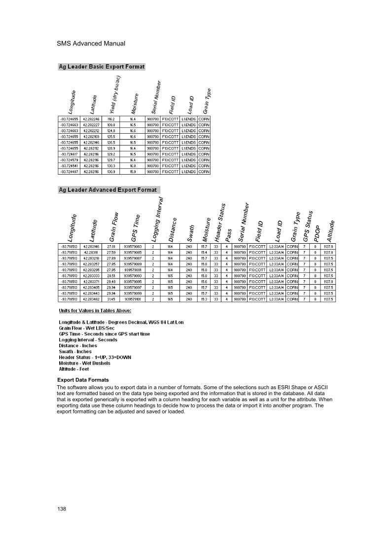
SMS Advanced Manual

138

Export Data FormatsThe software allows you to export data in a number of formats. Some of the selections such as ESRI Shape or ASCIItext are formatted based on the data type being exported and the information that is stored in the database. All datathat is exported generically is exported with a column heading for each variable as well as a unit for the attribute. Whenexporting data use these column headings to decide how to process the data or import it into another program. Theexport formatting can be adjusted and saved or loaded.

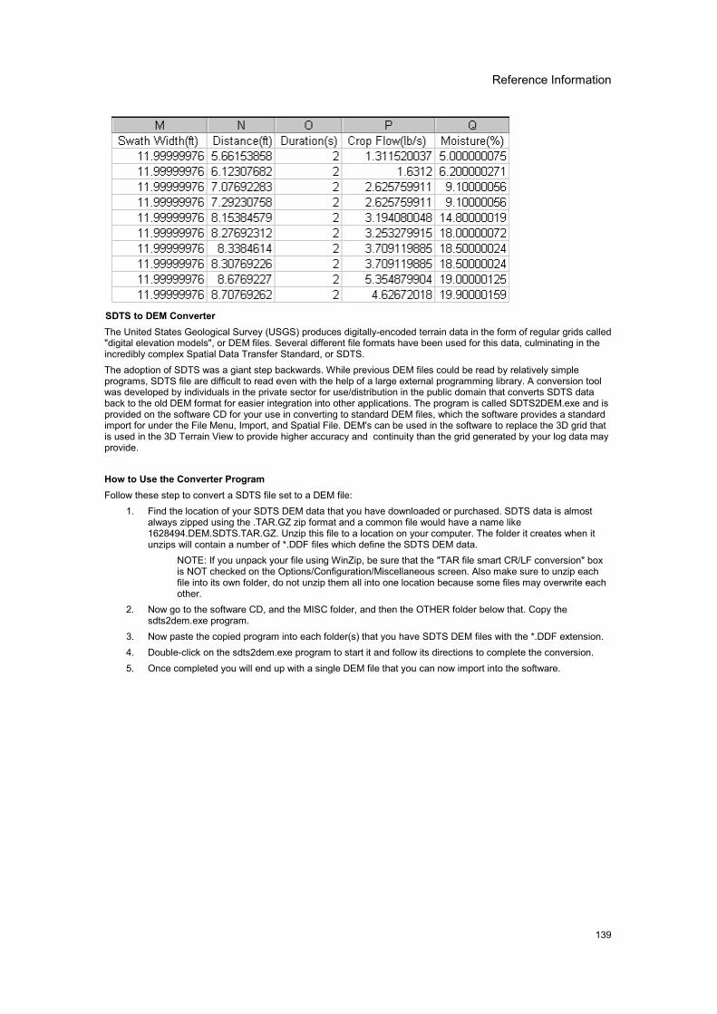
Reference Information

139

SDTS to DEM ConverterThe United States Geological Survey (USGS) produces digitally-encoded terrain data in the form of regular grids called"digital elevation models", or DEM files. Several different file formats have been used for this data, culminating in theincredibly complex Spatial Data Transfer Standard, or SDTS.The adoption of SDTS was a giant step backwards. While previous DEM files could be read by relatively simpleprograms, SDTS file are difficult to read even with the help of a large external programming library. A conversion toolwas developed by individuals in the private sector for use/distribution in the public domain that converts SDTS databack to the old DEM format for easier integration into other applications. The program is called SDTS2DEM.exe and isprovided on the software CD for your use in converting to standard DEM files, which the software provides a standardimport for under the File Menu, Import, and Spatial File. DEM's can be used in the software to replace the 3D grid thatis used in the 3D Terrain View to provide higher accuracy and continuity than the grid generated by your log data mayprovide.

How to Use the Converter ProgramFollow these step to convert a SDTS file set to a DEM file:

1. Find the location of your SDTS DEM data that you have downloaded or purchased. SDTS data is almostalways zipped using the .TAR.GZ zip format and a common file would have a name like1628494.DEM.SDTS.TAR.GZ. Unzip this file to a location on your computer. The folder it creates when itunzips will contain a number of *.DDF files which define the SDTS DEM data.

NOTE: If you unpack your file using WinZip, be sure that the "TAR file smart CR/LF conversion" boxis NOT checked on the Options/Configuration/Miscellaneous screen. Also make sure to unzip eachfile into its own folder, do not unzip them all into one location because some files may overwrite eachother.

2. Now go to the software CD, and the MISC folder, and then the OTHER folder below that. Copy thesdts2dem.exe program.

3. Now paste the copied program into each folder(s) that you have SDTS DEM files with the *.DDF extension.4. Double-click on the sdts2dem.exe program to start it and follow its directions to complete the conversion.5. Once completed you will end up with a single DEM file that you can now import into the software.

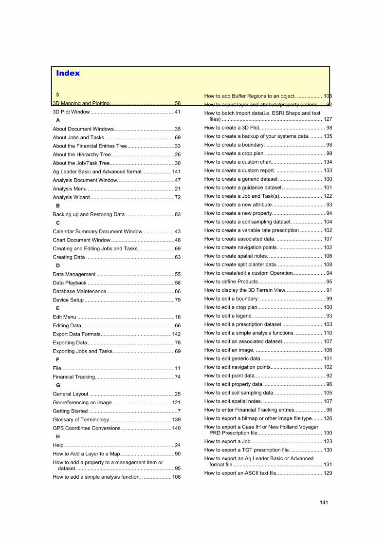
141

��$�

33D Mapping and Plotting............................................583D Plot Window .........................................................41AAbout Document Windows.........................................35About Jobs and Tasks ...............................................69About the Financial Entries Tree................................33About the Hierarchy Tree...........................................26About the Job/Task Tree............................................30Ag Leader Basic and Advanced format ....................141Analysis Document Window.......................................47Analysis Menu ...........................................................21Analysis Wizard .........................................................72BBacking up and Restoring Data .................................83CCalendar Summary Document Window .....................43Chart Document Window...........................................46Creating and Editing Jobs and Tasks.........................69Creating Data ............................................................63DData Management .....................................................55Data Playback ...........................................................58Database Maintenance..............................................86Device Setup .............................................................79EEdit Menu ..................................................................16Editing Data...............................................................66Export Data Formats................................................142Exporting Data...........................................................78Exporting Jobs and Tasks..........................................69FFile ............................................................................11Financial Tracking......................................................74GGeneral Layout ..........................................................25Georeferencing an Image ........................................121Getting Started ............................................................7Glossary of Terminology ..........................................139GPS Coordintes Conversions ..................................140HHelp...........................................................................24How to Add a Layer to a Map.....................................90How to add a property to a management item ordataset. ..................................................................95

How to add a simple analysis function. ....................108

How to add Buffer Regions to an object. ................. 106How to adjust layer and attribute/property options. .... 92How to batch import data(i.e. ESRI Shape,and textfiles) .................................................................... 127

How to create a 3D Plot. ........................................... 98How to create a backup of your systems data. ........ 135How to create a boundary. ........................................ 98How to create a crop plan. ........................................ 99How to create a custom chart.................................. 134How to create a custom report. ............................... 133How to create a generic dataset. ............................. 100How to create a guidance dataset. .......................... 101How to create a Job and Task(s)............................. 122How to create a new attribute.................................... 93How to create a new property.................................... 94How to create a soil sampling dataset. .................... 104How to create a variable rate prescription ............... 102How to create associated data. ............................... 107How to create navigation points. ............................. 102How to create spatial notes. .................................... 106How to create split planter data. .............................. 108How to create/edit a custom Operation...................... 94How to define Products ............................................. 95How to display the 3D Terrain View........................... 91How to edit a boundary. ............................................ 99How to edit a crop plan............................................ 100How to edit a legend. ................................................ 93How to edit a prescription dataset. .......................... 103How to edit a simple analysis functions. .................. 110How to edit an associated dataset........................... 107How to edit an image. ............................................. 106How to edit generic data.......................................... 101How to edit navigation points................................... 102How to edit point data................................................ 92How to edit property data. ......................................... 96How to edit soil sampling data................................. 105How to edit spatial notes. ........................................ 107How to enter Financial Tracking entries..................... 96How to export a bitmap or other image file type....... 126How to export a Case IH or New Holland VoyagerPRD Prescription file............................................ 130

How to export a Job. ............................................... 123How to export a TGT prescription file. ..................... 130How to export an Ag Leader Basic or Advancedformat file............................................................. 131

How to export an ASCII text file............................... 129

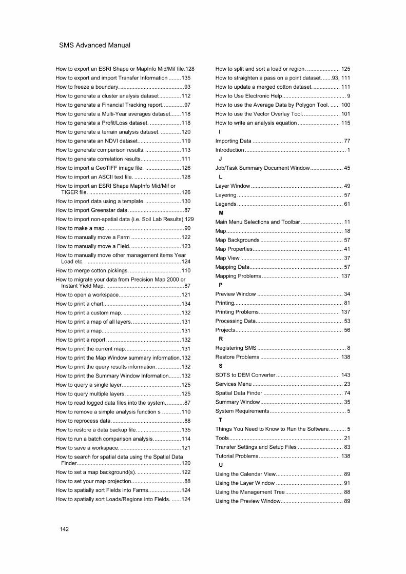
SMS Advanced Manual

142

How to export an ESRI Shape or MapInfo Mid/Mif file.128How to export and import Transfer Information ........135How to freeze a boundary. .........................................93How to generate a cluster analysis dataset ..............112How to generate a Financial Tracking report..............97How to generate a Multi-Year averages dataset.......118How to generate a Profit/Loss dataset. ....................118How to generate a terrain analysis dataset. .............120How to generate an NDVI dataset............................119How to generate comparison results. .......................113How to generate correlation results..........................111How to import a GeoTIFF image file. .......................126How to import an ASCII text file. ..............................128How to import an ESRI Shape MapInfo Mid/Mif orTIGER file. ...........................................................126

How to import data using a template........................130How to import Greenstar data. ...................................87How to import non-spatial data (i.e. Soil Lab Results).129How to make a map...................................................90How to manually move a Farm ................................122How to manually move a Field. ................................123How to manually move other management items YearLoad etc. . ............................................................124

How to merge cotton pickings. .................................110How to migrate your data from Precision Map 2000 orInstant Yield Map. ..................................................87

How to open a workspace........................................121How to print a chart..................................................134How to print a custom map. .....................................132How to print a map of all layers................................131How to print a map...................................................131How to print a report. ...............................................132How to print the current map....................................131How to print the Map Window summary information.132How to print the query results information. ...............132How to print the Summary Window Information........132How to query a single layer......................................125How to query multiple layers. ...................................125How to read logged data files into the system. ...........87How to remove a simple analysis function s ............110How to reprocess data. ..............................................88How to restore a data backup file.............................135How to run a batch comparison analysis. .................114How to save a workspace. .......................................121How to search for spatial data using the Spatial DataFinder...................................................................120

How to set a map background(s). ............................122How to set your map projection..................................88How to spatially sort Fields into Farms.....................124How to spatially sort Loads/Regions into Fields. ......124

How to split and sort a load or region. ..................... 125How to straighten a pass on a point dataset. ......93, 111How to update a merged cotton dataset. ................. 111How to Use Electronic Help......................................... 9How to use the Average Data by Polygon Tool. ...... 100How to use the Vector Overlay Tool. ....................... 101How to write an analysis equation ........................... 115IImporting Data .......................................................... 77Introduction ................................................................. 1JJob/Task Summary Document Window..................... 45LLayer Window ........................................................... 49Layering .................................................................... 57Legends .................................................................... 61MMain Menu Selections and Toolbar ........................... 11Map........................................................................... 18Map Backgrounds ..................................................... 57Map Properties.......................................................... 41Map View.................................................................. 37Mapping Data............................................................ 57Mapping Problems .................................................. 137PPreview Window ....................................................... 34Printing...................................................................... 81Printing Problems.................................................... 137Processing Data........................................................ 53Projects..................................................................... 56RRegistering SMS ......................................................... 8Restore Problems ................................................... 138SSDTS to DEM Converter ......................................... 143Services Menu .......................................................... 23Spatial Data Finder ................................................... 74Summary Window..................................................... 35System Requirements................................................. 5TThings You Need to Know to Run the Software........... 5Tools......................................................................... 21Transfer Settings and Setup Files ............................. 83Tutorial Problems.................................................... 138UUsing the Calendar View........................................... 89Using the Layer Window ........................................... 91Using the Management Tree..................................... 88Using the Preview Window........................................ 89

Index

143

VView ..........................................................................17

WWindow..................................................................... 24Workspaces .............................................................. 55

�