Social Identity and Preferences*

Daniel J. Benjamin

Cornell University and Institute for Social Research

James J. Choi Yale University and NBER

A. Joshua Strickland

Yale University

Current draft: August 1, 2007

Abstract In two laboratory experiments, we examine whether norms associated with one’s social identity affect time and risk preferences. When we make ethnic identity salient to Asian-American subjects, they make more patient choices. When we make race salient to black subjects, non-immigrant blacks (but not immigrant blacks) make more risk-averse choices. Making gender identity salient causes choices to conform to gender norms the subject believes are relatively more common. Our results provide evidence that identity effects play a role in shaping U.S. demographic patterns in economic behaviors and outcomes. JEL Classification: C91, Z10 Keywords: race, ethnicity, gender, identity, norm, stereotype, risk aversion, time preference * Experiment 1 was Strickland’s Harvard College honors senior thesis. We thank John Bargh, Nick Barberis, Jim Baron, Geoffrey Cohen, John Friedman, Matthew Gentzkow, Dan Gilbert, Moshe Hoffman, Emir Kamenica, Miles Kimball, Rachel Kranton, Ilyana Kuziemko, David Laibson, John List, Wendy Berry Mendes, Sendhil Mullainathan, Emily Oster, Todd Pittinsky, Claudia Sahm, Jesse Shapiro, Margaret Shih, Paul Tetlock, Rebecca Thornton, Robert Willis, and seminar participants at Harvard, Dartmouth, Michigan, Yale, and Chicago for comments and suggestions. We thank Bruce Rind for facilitating our access to Temple University. Sarah Bommarito, Gabriel Carroll, Josh Cherry, Ghim Chuan, Christopher Convery, Neals Frage, Bjorn Johnson, Dasol Kim, Annette Leung, Hans Lo, Shawn Nelson, Mark Petzold, Tiye Sherrod, Kimberly Solarz, Michael Stevens, Bernardo Vas, Narendra Vempati, and especially Neel Rao and Collin Raymond provided excellent research assistance. We thank the Russell Sage Foundation Small Grants Program in Behavioral Economics and the National Institute on Aging (grant P30-AG012810) for financial support. Benjamin acknowledges financial assistance from the Institute for Humane Studies, the Institute for Quantitative Social Science, the Program on Negotiation at Harvard Law School, Harvard’s Center for Justice, Welfare, and Economics, and the National Institute on Aging (grants T32-AG00186 and P01-AG26571). Choi acknowledges financial support from the Mustard Seed Foundation, the National Institute on Aging (grants R01-AG021650 and T32-AG00186), and Whitebox Advisors. Strickland thanks the Harvard College Research Program, the Harvard Economics Department, and the Harvard Psychology Department for financial assistance. E-mail: daniel.benjamin@gmail.com, james.choi@yale.edu, a.joshua.strickland@gmail.com.

2

I. Introduction

Economists have begun to theorize about how social identity matters for behavior

(Akerlof and Kranton, 2000, 2002, 2005; Fang and Loury, 2005; Bénabou and Tirole, 2006).

Building on a long tradition in the social sciences, Akerlof and Kranton (2000) propose that each

“social category” that constitutes part of an individual’s identity (such as Asian ethnicity, black

race, or male gender) is associated with a set of “norms” for how someone in that category

should behave (Bénabou and Tirole, 2006, propose a related theory). These norms influence

behavior because they affect the individual’s preferences. According to the theory, an individual

suffers disutility from deviating from his or her categories’ norms, which causes behavior to

conform toward those norms.

However, it is difficult to test with non-experimental data whether identity plays a causal

role in economic decision-making. In the field, social category affiliations are confounded with

many other factors such as socioeconomic status, opportunity sets, and peer pressure (Austen-

Smith and Fryer, 2005; Fryer and Torelli, 2005).

Social psychology offers a methodology for introducing exogenous variation in identity

effects. According to “self-categorization theory,” a long-standing idea in psychology (e.g.,

James, 1890; Turner, 1985), environmental cues called “primes” can temporarily make a certain

social category more salient, causing a person’s behavior to tilt more toward the norms

associated with the salient category. If the self-categorization theory is valid, then a researcher

can identify the effect of a particular social category on preferences by experimentally varying

the salience of the category and seeing how an individual’s behavior changes.

In this paper, we perform social-category-salience manipulations in the laboratory to test

the causal effect of ethnic, racial, and gender category norms on time and risk preferences. Many

social scientists have argued that differences in category norms regarding time and risk

preferences help explain ethnic, racial, and gender differences in capital accumulation and asset

allocation (Sowell, 1975, 1981, 2005; Murray, 1984; Chiswick, 1983; Barke, Jenkins-Smith, and

Slovic, 1997). For example, Sowell (1975, pp. 144-146) writes, “Among the characteristics

associated with success is a future orientation―a belief in a pattern of behavior that sacrifices

present comforts and enjoyments while preparing for future success… Those groups who [have

had] this―the Jews, the Japanese-Americans, and the West Indian Negroes, for example―all

3

came from social backgrounds in which this kind of behavior was common before they set foot

on American soil.”

We draw our category-salience manipulations from the psychology literature; for

example, we prime gender by asking experimental participants to list advantages of living in a

co-ed versus single-sex dorm (Shih, Pittinsky, and Ambady, 1999). Control subjects are instead

asked neutral questions unrelated to identity. We then elicit subjects’ time and risk preferences

using incentive-compatible mechanisms standard in experimental economics. We test whether

the effects of category norms on time and risk preferences are consistent with their contributing

to observed mean group differences in economic behavior.

Experiment 1 studies the effect of Asian ethnic category norms on time and risk

preferences. Relative to white Americans, Asian-Americans are more likely to participate in tax-

deferred savings accounts (Springstead and Wilson, 2000) and accumulate more human capital

(Sue and Okazaki, 1990). If Asian category norms help explain these patterns, then priming the

Asian identity category should cause Asian-American subjects to behave more patiently. We

make Asian identity salient by asking participants about their family background. Consistent

with the identity hypothesis, we find that primed Asian-American subjects make more patient

choices than Asian-American control subjects, requiring a much lower interest rate for delaying

receipt of payment. It is not clear what Asian risk aversion norm one would expect given the

existing empirical evidence, and we find that the ethnicity prime does not affect Asians’ risk

aversion. Asking about family background also has no effect on white subjects’ preferences. Our

first experiment’s findings suggest that identity effects on discount rates play a role in the high

financial and educational investment rates found among Asian-Americans.

Experiment 2 studies the effect of black racial category norms. Even after controlling for

other observable demographic variables, black Americans accumulate less financial wealth

(Altonji, Doraszelski, and Segal, 2000), accumulate less human capital (Neal and Johnson, 1996;

Fryer and Levitt, 2004), and are less likely to invest in the stock market (Hurst, Luoh, and

Stafford, 1998). However, black immigrants from the West Indies and Africa are

disproportionately represented among high-income blacks and elite college students (Sowell,

1975; Rimer and Arenson, 2004). If these group differences are a result of identity-induced

differences in preferences, then priming the racial identity category should cause native blacks—

but not immigrant blacks—to become less patient (explaining lower capital accumulation), more

4

risk averse (explaining lower investment in stocks and other assets commanding positive risk

premia, and hence lower long-run capital accumulation), or both. We make racial identity salient

to white and black participants by asking questions about living with individuals of the same or

different races. Inconsistent with Sowell’s hypothesis, we do not find significant identity-related

discount rate differences between native blacks, immigrant blacks, and whites. However, we do

find identity-related risk aversion effects for black subjects that depend upon how recently their

family immigrated to the United States. Blacks with longstanding U.S. roots become more risk-

averse when primed. In contrast, blacks who have at least one foreign-born parent or who are

themselves foreign-born appear, if anything, to become less risk averse. White risk aversion is

unaffected by the prime. These results suggest that racial risk norms depress native blacks’

capital accumulation and stock market participation.

Experiment 2 also examines gender category norms. Since women invest in more

conservative financial assets than men (Jianakoplos and Bernasek, 1998; Sundén and Surette,

1998) and behave more cautiously in laboratory experiments (Croson and Gneezy, 2004; Byrnes,

Miller, and Schaefer, 1999), one might expect that priming the gender category would cause

women to become more risk averse and men to become less risk averse. We do not find a mean

difference in gender identity effects on either discount rates or risk aversion. Nevertheless,

subjects do conform to the norms they believe apply to their gender. Priming gender increases

risk aversion among men who believe that cautious stereotypes about men are relatively more

common. Priming gender decreases risk aversion in women who believe that reckless stereotypes

about women are relatively more common. These effects reverse for those who hold opposite

beliefs about the stereotypes. Analogously, we find that gender-primed subjects conform to the

risk-aversion norm they believe children of their gender are told they should adhere to. Gender-

primed women also conform to the patience norm they believe girls are told they should obey.

We interpret our results within the framework of the psychology literature on identity

salience, according to which priming an identity category causes individuals to conform to the

category’s social prescriptions. However, a potential alternative interpretation comes from the

psychology literature on “stereotype threat,” which argues that making members of

disadvantaged groups more aware of negative stereotypes about them causes them to become

anxious, disrupting cognitive processing and impairing performance on standardized tests (e.g.,

Steele and Aronson, 1995; Shih, Pittinsky, and Ambady, 1999; Hoff and Pandey, 2006; Marx

5

and Stapel, 2006a). This reduction in cognitive resources could lead to less patient and more

risk-averse behavior (Benjamin, Brown, and Shapiro, 2006). Conversely, “stereotype lift”

increases cognitive performance of a group when negative stereotypes about other groups are

made salient (Walton and Cohen, 2003; Marx and Stapel, 2006b), which may in itself engender

more patient and less risk-averse behavior (Benjamin, Brown, and Shapiro, 2006). However, a

necessary condition for the stereotype threat or lift mechanism to operate is that subjects perceive

the task to be diagnostic of ability (Croizet and Claire, 1998; Aronson, Quinn, and Spencer,

1998; Kray, Thompson, and Galinsky, 2001). In order to avoid inducing stereotype threat or lift,

we did not present the choice tasks as diagnostic. In our second experiment, we explicitly

described the choice tasks as “a matter of personal preference” with “no right or wrong answers.”

We also had subjects in our second experiment answer five SAT-style math questions after their

preferences were elicited. Primed subjects did not perform differently than unprimed subjects,

suggesting that our priming manipulation did not affect cognitive performance.

There is a large literature in psychology on identity salience. For example, psychologists

have shown that identity salience affects preferences elicited hypothetically over highbrow

versus lowbrow activities, (Chinese) collectivist versus (American) individualist behavior, and

professional- versus family-oriented activities (LeBoeuf, Shafir, and Belyavsky, 2006); animal

vivisection and ethically questionable experimentation (Reicher and Levine, 1994); and

ethnically targeted advertising (Forehand, Deshpandé, and Reed, 2002). Relative to the

psychology literature, our work differs by focusing on primitive preference parameters measured

with incentive-compatible mechanisms, dependent variables that are primarily of interest to

economists.

The paper is organized as followed. Section II describes a theoretical framework for

understanding identity and priming effects. Section III presents the first experiment, which

studies ethnic priming effects among Asian-Americans. Section IV presents the second

experiment, which studies racial priming effects among blacks and gender priming effects.

Section V concludes the paper.

II. A Theoretical Framework

In this section, we outline a theoretical framework inspired by Akerlof and Kranton

(2000) that organizes our thinking about identity and priming effects. In this framework, priming

6

a particular social category reveals the marginal effect of increasing the strength of affiliation

with that category.

Let x be some decision variable, such as how much to pursue immediate gratification or

how much to avoid risks (so that higher choice of x corresponds to a higher discount rate

parameter or higher risk aversion parameter, respectively). An individual belongs to some social

category C, such as black race or female gender, with strength s > 0. Let 0x denote the optimal

choice of x without identity considerations, and let xC denote the norm associated with social

category C—that is, the choice of x prescribed for members of C. The individual chooses x to

maximize

2 20(1 ( ))( ) ( )( )CU w s x x w s x x= − − − − − , (1)

where 0 ≤ w(s) ≤ 1 is the weight placed on social category C in the person's decision. We assume

that w(0) = 0 and w′ > 0. Deviating from the norm prescribed for one’s category causes disutility

that is increasing in s, the strength of one’s affiliation with that category. For simplicity, we

analyze the case where only a single social category is relevant to an individual, but it would be

straightforward to add terms to the utility function reflecting other identities the individual holds.

We assume that s has a steady-state value s but can be temporarily perturbed away from

s by a category prime ε; for example, s might follow an AR(1) process, 1(1 )t t ts s sφ φ ε−= − + + .

The first-order condition of (1) gives the optimal action,

*0( ) (1 ( )) ( ) ,Cx s w s x w s x= − + (2)

which is a weighted average of the optimal choice without identity considerations and the

category norm. This condition yields several implications that guide our analysis.

Proposition 1: The higher the steady-state strength s of the category affiliation, the closer *x is

to xC.

Proposition 2: A category prime ε > 0 (whether naturally occurring or experimentally induced)

also causes *x to move closer to xC.

7

Thus, the behavioral effect of priming social category C reveals the marginal behavioral effect of

increasing the steady-state strength s of category C. This is why priming manipulations are a

useful experimental procedure for studying identity effects.

Proposition 3: The derivative

*

0'( )( )Cdx w s x xds

= − (3)

depends on the sign of 0Cx x− .

Even if college students differ from the general population in the shape of their w(s) function and

their levels of s and 0x , the directional effects of priming on college students will generalize as

long as 0Cx x− has the same sign on average for both groups.

Many psychologists have expressed the intuition that priming a category should have a

stronger effect on those who identify more strongly with that category. For example, LeBoeuf,

Shafir, and Belyavsky (2006, p.19) hypothesize that “evoking an identity will trigger preference

assimilation only for those highly identified with that identity.” In our framework, suppose

without loss of generality that 0 Cx x< . Then the hypothesis of increasing sensitivity to priming

corresponds to the condition *d dx

ds ds⎛ ⎞⎜ ⎟⎝ ⎠

0''( )( ) 0Cw s x x= − > . Our formal framework generates a

perhaps surprising conclusion about the interaction between priming and category affiliation

strength.

Proposition 4: In general it is ambiguous whether the priming effect is stronger or weaker for

individuals with a stronger category affiliation. Suppose, without loss of generality, that 0 Cx x< .

Then 2 *

2 0d xds

> if and only if ( ) 0w s′′ > .

Depending on the shape of ( )w ⋅ and the level of s, 2 * 2/d x ds could take either sign. Intuitively,

while it may be the case that individuals with higher s are more susceptible to priming ( 0w′′ > ),

it could instead be that such individuals become saturated with the category norm ( 0w′′ < ). For

8

that reason, even though we report interaction effects between priming effects and identification

strength, we do not emphasize those empirical results.

In summary, the behavioral response to priming a social category provides directional

information about the norms associated with that category, but both the magnitude of the effect

and its interaction with affiliation strength must be interpreted cautiously. In the remainder of

this paper, we employ category-salience experiments to uncover norms associated with Asian

ethnicity, black race, and male and female gender.

III. Experiment 1: Asian-American Ethnic Norms

Asian-Americans are more likely to participate in tax-deferred savings accounts

(Springstead and Wilson, 2000) and accumulate more human capital (Sue and Okazaki, 1990)

than white Americans.1 Norms for patient behavior seem to be linked to many Asian ethnic

identities. American stereotypes about East Asian patience and industriousness date back to at

least the 19th century (Twain, 1872)2 and persist to this day (e.g., Kasindorf, 1982; Abboud and

Kim, 2005). Although there are differences between Asian cultures, Hofstede and Bond (1988)

argue that most are high in “Confucian Dynamism,” which emphasizes a “future-oriented

mentality.” If identity effects on discount rates play a role in raising Asian-American financial

and educational investment rates, then priming the Asian identity category should cause Asian-

American subjects to behave more patiently.

We also measured how priming the Asian identity category affects risk aversion,

although it is unclear what risk preference norm one should expect to find associated with Asian-

American ethnicity. Barsky et al. (1997) find that Asian-Americans answer hypothetical survey

questions in a less risk-averse manner than whites, and Weber and Hsee (1998) and Hsee and

Weber (1999) present evidence that Chinese experimental subjects in the People’s Republic of

China are less risk averse than American subjects, suggesting that there may be a risk-tolerant

Asian category norm. On the other hand, both Chinese and American subjects in Hsee and

1 It should be noted that Carroll, Rhee, and Rhee (1994, 1999) do not find that Asian immigrants save more, but they are hindered by their data quality. However, Carroll, Rhee, and Rhee (1994) do find that Asian-Canadian immigrants’ educational expenditures are 3.6 times the Canadian average. 2 Twain wrote, “They are quiet, peaceable, tractable, free from drunkenness, and they are as industrious as the day is long. A disorderly Chinaman is rare, and a lazy one does not exist... Chinamen make good house servants, being quick, obedient, patient, quick to learn and tirelessly industrious.”

9

Weber (1999) believed that Americans would be more risk seeking, and Hong (1978) finds that

Chinese experimental subjects in Taiwan are more risk averse than American subjects.

We used the method developed by Shih, Pittinsky, and Ambady (1999) to prime the

Asian ethnic identity category in Asian-American subjects. We then elicited time and risk

preferences from primed and unprimed subjects using an incentive-compatible mechanism. To

check that any Asian priming effect is working through the increase salience of the Asian ethnic

identity category, we applied the same prime to white subjects.

A. Participants

Participants were 159 Harvard College undergraduates, 71 of Asian descent and 66 of

white descent. We drop from our analysis three biracial participants and 18 participants who

were neither white nor Asian. Within our Asian group, 90% were of East Asian descent, and the

remainder were of Asian Indian descent.3 All of our Asian identity results continue to hold if we

drop Asian Indians from the sample.

We recruited participants by putting up posters in the Harvard psychology building, e-

mailing students who reported being members of undergraduate Asian-American clubs on

Facebook.com, and e-mailing Harvard dormitory lists. There were a small number of subjects

who walked into experimental sessions upon observing that they were about to start. At no point

did we specify in our recruiting materials that we were looking for white and Asian students.

B. Procedure

The experimenter, a male of black, Mexican, and white descent, ran 15-minute sessions

with groups of between one and ten subjects from December 2004 to February 2005. Half the

participants were randomly assigned to the ethnicity-salience condition and half to the control

condition. At the onset of the experiment, the same instructions describing the experiment and its

compensation scheme were read to every subject. Subjects then responded to three sections of

questions. As they completed each section, they continued without interruption to the next one.

The first section was a “background questionnaire” that varied by experimental condition. The

second section elicited participants’ time preferences. The third section elicited their risk

3 Specifically, there were 41 Chinese, 7 Indians, 7 Koreans, 5 Taiwanese, 2 Japanese, 1 Filipino, 1 Thai, 1 Vietnamese, and 6 unspecified Asians.

10

preferences. Finally, participants were debriefed, their race was recorded, and payments were

made.

Ethnicity-salience manipulation. In the ethnicity-salience condition, there were eight questions in

the “background questionnaire”:

(a) What year in school are you?

(b) Do you live on or off campus?

(c) Do your parents or grandparents speak any languages other than English?

(d) What languages do you know?

(e) What opportunities do you have to speak these languages around campus?

(f) What percentage of these opportunities is found in the residence halls?

(g) What language do you speak at home?

(h) How many generations of your family have lived in the United States?

Questions (c) through (h) are exactly those used by Shih, Pittinsky, and Ambady (1999) to make

ethnicity salient to Asian-Americans. Questions (a) and (b) were added to disguise the

questionnaire’s intent.

Control condition. In the control condition, the “background questionnaire” began with the same

two questions as the ethnicity-salience questionnaire. The remaining six questions were designed

to be neutral with respect to ethnic identity:

(a) What year in school are you?

(b) Do you live on or off campus?

(c) How many meals a week do you eat in the residence dining halls?

(d) From 1 to 7 how satisfied would you say you are with the food?

(e) If a limited-meals meal plan were offered would it interest you?

(f) Would you consider subscribing to cable television if it was offered?

(g) How much would you be willing to pay per month for this service?

(h) List one or two reasons why you would or would not subscribe to cable television.

These questions are modeled after the control questions of Shih, Pittinsky, and Ambady (1999),

modified to be relevant for current issues faced by the Harvard student body.

11

Measured time preferences. We measured time preferences by asking participants to make a

series of binary choices between money received at different times. Each choice had some

probability of determining their actual payment. The choices were divided into two 11-question

blocks and two 12-question blocks. One of the 11-question blocks required participants to circle

either “$3 today or X in 1 week,” where X = $3.05, $3.10, $3.25, $3.50, $3.75, $4.00, $4.50,

$5.00, $5.50, $6.00, or $7.00. The other 11-question block asked about “$3 in 1 week or X in 2

weeks,” where X took on the same values as in the first block. The 12-question blocks were the

same as the first two, except that the monetary amounts were larger. The immediate reward was

$7, and the delayed rewards took values X = $7.10, $7.25, $7.50, $8.00, $8.50, $9.25, $10.00,

$10.75, $11.75, $12.50, $13.75, or $15.00. Half the participants saw the questions in ascending

order of X, and half in descending order. Half answered the today versus one week questions

before the one week versus two weeks questions, and half the other way around. It took

participants around five minutes to answer the time preference questions.

Even though our approach to measuring time preferences is standard (Frederick,

Loewenstein, and O’Donoghue, 2002), it has been argued that choices over the timing of

monetary rewards should not measure time preference, since people can (in principle) borrow or

lend money at the market interest rate regardless of how they discount future utility (Fuchs,

1982). However, in experiments like ours, there is in fact substantial heterogeneity in measured

discount rates, and most participants discount future rewards at a much higher rate than the

market interest rate (Frederick, Loewenstein, and O’Donoghue 2002), perhaps because they are

liquidity-constrained or do not realize that money is fungible. In either case, questions involving

monetary rewards do appear to measure discounting over utility. Consistent with this

interpretation, time preference measured in a manner similar to ours predicts variation in

discounting-related behaviors such as drug addiction (e.g., Kirby, Petry, and Bickel, 1999; Kirby

and Petry, 2004), cigarette smoking (Fuchs, 1982; Bickel, Odum, and Madden, 1999), excessive

gambling (Petry and Casarella, 1999), use of commitment savings devices (Ashraf, Karlan, and

Yin, 2006), borrowing on installment accounts and credit cards (Meier and Sprenger, 2006), and

rapid exhaustion of food stamps (Shapiro, 2005).4

4 Some economists are troubled by the fact that subjects in experiments such as ours require extremely high interest rates to delay payment receipt. For example, a subject choosing to receive $3 today rather than $3.05 in one week is borrowing at an annualized interest rate of 136%. Although it is difficult to believe that such impatience is

12

Measured risk preferences. We measured risk preferences with 18 binary choices between a safe

option and a gamble: “$4 guaranteed or a Y% chance at $8.” Y took all values from 25% through

76% in increments of 3%. Half the participants saw the questions in order of ascending Y and

half in descending order. Each binary choice had some probability of determining the

participant’s payout. If a risk preference choice was selected for payment, the payment was

immediate (as opposed to delayed by one or two weeks). Answering these questions took about

three minutes.

Existing evidence suggests that risk preferences measured through laboratory choice

tasks are related to real-world risk behaviors. Risk aversion measures derived from real-stakes

experimental choices are highly correlated with measures from hypothetical choices (Dohmen et

al., 2005), which in turn predict risky behaviors such as smoking, drinking, failing to hold

insurance, holding stocks rather than Treasury bills, being self-employed, switching jobs, and

moving residences (Barsky et al., 1997; Guiso and Paiella, 2001; Dohmen et al., 2005; Sahm,

2007).

Compensation scheme. Before the participant answered any of the preference elicitation

questions, the experimenter explained that at the end of the experiment, the participant would

randomly select which one of the time or risk preference choices would determine his or her

payout by drawing a number out of a bag.5 The bag contained slips of paper numbered 1 to 64,

one for each preference elicitation question. If a risk preference question was selected, and if the

participant had chosen the gamble in that question, then the participant would randomly draw a

number out of a different bag, which contained numbers between 1 and 100. If the drawn number

was less than or equal to the Y% probability of winning, the participant won $8.6

normatively justified, the real-world payday loan market typically features a two-week interest rate of 18% (Morse, 2006; Skiba and Tobacman, 2007), which annualizes to 7295%. 5 Existing evidence suggests that paying subjects for a randomly-chosen question causes subjects to behave as if they were being paid for every question (Hey and Lee, 2005; Laury, 2005). 6 The printed instructions on the risk elicitation sheet stated that gambles would be resolved by drawing from a bag of red and blue marbles, which had been the original intention, but which proved logistically impractical.

13

All rewards were paid by a check given to the participant immediately following the

debriefing. Delayed payments were implemented by post-dating the check. Subjects were told

the post-dated check could not be cashed until the date on the check.7

C. Econometric methodology

In our time preference task, we would like to use as our dependent variable the minimum

continuously compounded weekly interest rate that the subject requires to choose the later

payment over the earlier payment (i.e., the reservation price for accepting later payment). For

example, if the subject would choose the later payment over an earlier $3 payment if and only if

the later payment is at least $3.50, then the reservation interest rate is r = log(3.50/3) = 0.154.

Similarly, in our risk preference task, we would like to use as our dependent variable the

minimum expected return premium that the subject requires to accept the gamble over the certain

payout. For example, if the subject would choose to gamble for $8 rather than accept the sure $4

if and only if the probability of winning is at least 58%, then the reservation risk premium is π =

(8 × 0.58 – 4)/4 = 0.16.

In reality, we observe choices at only a finite number of interest rates and risk premia,

and there are a substantial number of subjects whose observations are left- or right-censored.

Therefore, if the subject chooses the earlier $3 payment over the later $3.25 payment, but the

later $3.50 payment over the earlier $3 payment, we only know that her r is between log(3.25/3)

and log(3.50/3). A similar problem applies to the risk choices. We therefore use an interval

regression (Stewart, 1983), which is a maximum-likelihood procedure that assumes that the

latent dependent variable is conditionally distributed normally, has an unknown exact value, but

is known to fall within a certain interval.8

7 To secure the promise to pay at the end of a loan term, payday lending companies typically use postdated checks collected from borrowers at the time of loan origination (Potter, 2002). Although a check-issuer’s bank bears no legal liability if it pays a postdated check early (provided the check-writer did not notify the bank of the check in advance; see U.C.C. §4-401), many banks will not allow account holders to deposit post-dated checks. Although we did not keep track of check deposit dates in Experiment 1, we found in Experiment 2’s Temple sample that almost all subjects deposited their checks after the check date. (Because of how we ensured anonymity, a similar analysis in Experiment 2’s Michigan sample was impossible.) All but one participant deposited his or her check into a bank checking account. 8 Only two subjects did not have a threshold such that they chose the earlier payment if and only if the interest rate was below that threshold. These two subjects also did not have a risk premium threshold such that they chose the certain payoff if and only if the risk premium was below that threshold. Our results are unaffected by excluding these two subjects. In our analysis, we use the interval corresponding to the lowest interest rate and lowest risk premium at which the subject behaved impatiently or risk-aversely, respectively.

14

The normality assumption implies that the dependent variable sometimes takes on

negative values. This negativity is not a problem in the risk preference regressions, since we do

observe some risk-seeking behavior in our data. We therefore use π as the dependent variable in

the risk preference regressions. However, our prior belief is that negative interest rates, if they

were measured in our experiment, would be perverse and likely due to elicitation errors.

Therefore, we impose lognormality on the interest rate variable by making log(r) the dependent

variable in the interval regression, thus ruling out negative interest rates. In the interest rate

regression tables that follow, if the coefficients imply that a certain set of explanatory variable

values are associated with a mean log(r) of μ̂ , then the median r is ˆexp( )μ . Because of outliers,

we will focus on median interest rates in our analysis.9

We observe four r (interval) values for each participant, since we elicited four sets of

intertemporal preferences. In the time preference results that follow, we report results that pool

the four r values together, adding explanatory dummy variables to indicate for which trade-off

type (now versus one week, one week versus two weeks, small intertemporal choice, larger

intertemporal choice) the r value was observed. We cluster standard errors by subject to correct

for within-subject correlation of r (Froot, 1989; Rogers, 1993).

D. Results

Of the participants who received the priming manipulation, 92% of the Asians reported

having families who lived in the U.S. for two or fewer generations, and 84% reported a non-

English language spoken at home. In contrast, only 36% of the primed white subjects had

families who lived in the U.S. for two or fewer generations, and a mere 3% had homes where a

non-English language was spoken. Therefore, the priming questions may not have made

ethnicity salient to many white participants. Nonetheless, comparing the effect of the

manipulation on white versus Asian participants allows us to check that any priming effect on

the Asians is working through the increased salience of the Asian ethnic identity category, rather

than through some other channel that would affect the whites as well.

In total, each subject made 46 intertemporal choices (pooling across stake sizes and

horizons) and 18 risk choices. Table 1 displays, by experimental condition and race, the average 9 The mean r is ˆ ˆexp( 0.5 )μ σ+ , where σ̂ is the (estimated) conditional standard deviation of the log(r) distribution. Outliers make this mean quite large for many experimental groups. However, the point estimates for the priming effects are directionally similar when we focus on mean interest rates.

15

proportion of those choices where subjects chose the earlier or safe option. First examining

choices in the unprimed condition, the Asian participants are somewhat more impatient and risk

averse than the white participants. This non-experimental comparison is confounded by sample

selection (both into the Harvard student body and into the experiment); in the nationally

representative Health and Retirement Study, middle-aged and older Asian-Americans appear to

be less risk averse than whites on average (Barsky et al., 1997). To learn about identity effects,

we instead turn to the comparison between treatment and control groups.

Even though Table 1 discards all information about the prices involved in each trade-off,

the main result of Experiment 1 is immediately apparent: Asians make significantly fewer

impatient choices when their ethnicity is primed. The 14 percentage point drop in the proportion

of impatient choices is significant at the 1% level. In contrast, whites seem to get slightly more

impatient in the ethnic prime condition, but the difference is not significant. Neither whites nor

Asians change their risk choices in response to the ethnicity prime.

Table 2 presents formal regression evidence on priming effects. We regress participants’

required log interest rate and risk premium on experimental condition and trade-off type. Column

1 confirms what we saw in the first table: the interest rate required by Asians to defer payment

falls dramatically when Asian ethnic identity is made salient. For example, for trade-offs

between $4 now and money one week from now, the median required interest rate falls from

8.8% to 2.1%. Running separate regressions for each intertemporal choice type (immediate

payment amount × time horizon) reveals that this treatment effect is statistically significant at the

1% level and of similar magnitude for all four types (not shown in tables). Column 3 shows that

there is no effect on the risk premium Asians require to accept gambles. Columns 2 and 4 show,

in analogous regressions for white subjects, that whites’ choices are not affected by the prime.10

IV. Experiment 2: Black Racial Norms and Gender Norms

While Experiment 1 focused on Asian ethnic category norms, Experiment 2 explores how

preferences are affected by black racial category norms and gender category norms. Sowell

(1975, 1981, 2001) and Murray (1984) have argued that black category norms encourage 10 It would be interesting to examine whether primed Asians who have been in the U.S. for one or fewer generations, who report speaking only an Asian language at home, or who list an Asian language first when asked what languages they know demand especially low interest rates. However, we are hampered by our not having collected these affiliation strength data for the control group, preventing us from controlling for baseline preference differences correlated with differing affiliation strength.

16

impatient behavior. Yankelovich Partners Inc. (1999) describes a “culture of conservatism”

among higher-income blacks with regards to investing, which accords with Sahm’s (2007)

finding that, controlling for demographics, blacks in the Health and Retirement Study are

significantly more risk averse over hypothetical wealth gambles than whites. If identity-related

differences in time or risk preferences explain why black Americans accumulate less financial

wealth (Altonji, Doraszelski, and Segal, 2000), accumulate less human capital (Neal and

Johnson, 1996; Fryer and Levitt, 2004), and are less likely to invest in the stock market (Hurst,

Luoh, and Stafford, 1998) than white Americans, then we expect that priming the racial identity

category among American-born blacks should increase discount rates, increase risk aversion, or

both.11

Immigrant blacks—defined as blacks who were born abroad or who have at least one

parent who was born abroad—comprise a substantial minority (41%) of our black participants.

Sociological research indicates that blacks whose families have recently immigrated to the U.S.

grow up with a very different cultural heritage than blacks whose families have long-standing

U.S. roots (e.g., Waters, 1994). Because black immigrants from the West Indies and Africa are

disproportionately represented among high-income blacks and elite college students (Sowell,

1975; Rimer and Arenson, 2004), and often identify themselves in contrast to American-born

blacks (Waters, 1994), we examined whether the effects of priming race on immigrant blacks

differ from the priming effects on blacks with long-standing U.S. roots.

Finally, because women invest in more conservative financial assets than men

(Jianakoplos and Bernasek, 1998; Sundén and Surette, 1998) and act more cautiously in

laboratory experiments (Croson and Gneezy, 2004; Byrnes, Miller, and Schaefer, 1999), we

tested whether priming gender would cause women to become more risk averse and men to

become less risk averse.

Experiment 2 also expanded on the earlier experiment by measuring larger-stakes (in

addition to small-stakes) risk preferences and by asking a host of questions that would enable us

to test potential mechanisms underlying the category-salience effects. In addition, we introduced

variation in the delay between the salience manipulation and the preference elicitations, which

allows us to investigate the impulse response function of a category-salience shock.

11 On the other hand, blacks seem to be more likely to engage in risky health behaviors than whites (Hahn, Vesely, and Chang, 2000), perhaps suggesting that black identity is associated with a risk-seeking norm, at least in the health domain.

17

A. Participants

We recruited 280 Temple University students by handing out flyers on campus and

providing a $1 referral fee to participants for each friend they got to sign up for the experiment.

We recruited 231 University of Michigan students by handing out flyers, putting up posters, and

e-mailing student groups likely to have many black members.12 In order to avoid pre-priming

participants with their racial identity category, we did not at any point mention that we were

looking for black and white subjects. There were 128 black subjects, 296 non-Hispanic white

subjects, and 87 subjects who were neither black nor non-Hispanic white. Among our

participants, 44% were male.

B. Procedure

We conducted 19 fifty-minute experimental sessions in Temple classrooms on March 18,

25, and 26 of 2006. The smallest session had 6 participants, and the largest had 29. We also

conducted 28 sessions at the University of Michigan between November 30, 2006, and April 10,

2007. There were 2 participants in the smallest session and 28 in the largest. Our results from the

Temple and Michigan samples are directionally similar, so we pool them in all analyses.

We randomly assigned participants to the race-salience, gender-salience, or control

conditions. Because of the scarcity of black subjects, we did not assign any black participants to

the gender-salience condition.

The principal experimenter for the Temple sessions was a male of black, Mexican, and

white descent. He was assisted by a white male and an Asian male. The Michigan sessions were

conducted by various experimenters of white, black, Hispanic, and Asian descent and both

genders.13

12 We initially ran the experiment at Temple University because it has one of the largest black student populations (approximately 20% of the 34,000 students) in the United States outside of the historically black colleges. Running the experiment at an historically black college would have precluded our recruiting white subjects from the same population, and we worried that students at historically black colleges may be so saturated with their racial identity category that a priming manipulation would have no measurable additional effect. We ran additional sessions at Michigan in order to generate out-of-sample evidence of the Temple priming effects and to measure the effect of norms communicated through childhood messages. 13 Although we have little power to test directly for experimenter race and gender effects, the fact that the Temple and Michigan results are directionally similar when analyzed separately suggests that these effects were not an important factor for our results.

18

After the questionnaire booklet was distributed to each participant, the principal

experimenter guided session participants through the questionnaire together by reading

instructions aloud before each section. The questionnaire was divided into sections (with the

neutral labels “Section 1,” “Section 2,” and so on). The first section contained the category-

salience manipulation or control. The next three sections were a time preference elicitation

(which took 5 minutes for instructions and responses), a risk preference elicitation (5 minutes),

and a six-question version of the Spielberger State-Trait Anxiety Inventory (Marteau and

Bekker, 1992) (1.5 minutes). These three sections’ order varied across sessions. The penultimate

section was a six-question math quiz with SAT-like questions. The questionnaire’s final section

asked a variety of questions about personal and family background, as well as questions

unrelated to the study in order to mask its purpose.14 Each of the time and risk preference

measures was incentive-compatible, as explained below. We also paid subjects 10 cents for each

math question they answered correctly. Participants were paid for their choices, plus a $1 show-

up fee, by check immediately upon completing the experiment. In order to avoid contaminating

future subjects, participants’ debriefing form did not reveal that our study was about race and

gender.15

Race-salience manipulation. In the race-salience condition, we adapted for race the questions

that Shih, Pittinsky, and Ambady (1999) used to make gender salient. Specifically, we asked

participants the following in the questionnaire’s first section:

(a) Do you live on campus or off campus?

(b) Do you have a roommate?

(c) What is your race?

(d) If you could live with any roommate you liked, would you prefer to live with a

roommate of your own race or a different race?

(e) Please list three advantages of having a roommate of your own race.

(f) Please list three advantages of having a roommate of a different race.

14 In addition to asking subjects to report their race and gender, we surreptitiously recorded most subjects’ race and gender during the experimental sessions. We relied on subjects’ self-reported race and gender except in one case where it seemed clear both from our visual observation and from other parts of the questionnaire that the subject had accidentally circled the wrong gender. 15 When all sessions were completed, we provided subjects a more complete debriefing via e-mail.

19

Gender-salience manipulation. In the gender-salience condition, the questions in the first section

were nearly identical16 to those that Shih, Pittinsky, and Ambady (1999) used to make gender

salient:

(a) Do you live on campus or off campus?

(b) Do you have a roommate?

(c) What is your gender?

(d) If you could live anywhere on campus, would you prefer living on a co-ed floor or a

single-sex floor?

(e) Please list three advantages of living on a co-ed floor.

(f) Please list three advantages of living on a single-sex floor.

Control condition. In the control condition, the first section asked participants questions designed

not to make either race or gender salient, but which followed a structure parallel to the race- and

gender-salience questions:

(a) Do you live on campus or off campus?

(b) Do you have a roommate?

(c) How old are you?

(d) If you could live anywhere, would you prefer to live on campus or off campus?

(e) Please list three advantages of living on campus.

(f) Please list three advantages of living off campus.

Measured time preferences. We measured time preferences by asking participants to make two

sets of 12 binary choices. In the first set of 12 questions, the participant was asked to circle either

“(A) I prefer to get $10 right now,” or “(B) I prefer to get X one week from now,” where X =

$10.10, $10.25, $10.50, $10.75, $11.00, $11.25, $11.50, $12.00, $12.50, $13, $14, and $15. The

second set of 12 questions was the same as the first set, except that option (A) occurred “one

week from now,” and option (B) occurred “two weeks from now.” These questions were

presented with the delayed reward X in ascending order.

16 Shih, Pittinsky, and Ambady (1999) do not ask the subjects’ gender in their gender prime. In addition, we slightly rephrased question (d) to remove some potential ambiguity in the analogous question used by Shih et al.

20

The section’s instructions gave two sample questions and explained that later during the

experiment, a participant would roll a 24-sided die to determine which question would count for

payment in that session. All payments would be made by checks given to subjects immediately

after the session, and if on the chosen question the subject had selected the delayed payment, he

would receive that delayed payment as a post-dated check. The experimenter told participants

that post-dated checks can be cashed any time on or after the check’s date.17 The final two

sentences of the section’s instructions made clear that the questions were not intended to evaluate

performance: “It’s important to keep in mind that there are no right or wrong answers here.

Which choice you make is a matter of personal preference.” (We used this same wording again

in the instructions for both risk preference sections.)

Measured risk preferences. One section of the questionnaire measured risk preferences. This

section was split into a portion measuring risk preferences over small stakes and a portion

measuring risk preferences over larger stakes.

We elicited small-stakes risk preferences by asking participants to circle either “(A) I get

$1 for sure,” or “(B) If the six-sided die comes up 1, 2, or 3, I get X. If the six-sided die comes up

4, 5, or 6, I get nothing.” We asked six such questions, where X = $1.60, $2, $2.40, $2.80, $3.20,

and $3.60. The questions were presented in ascending order of X.

The small-stakes section’s instructions gave a sample question and told participants that

they would be paid according to every choice they made in the small-stakes risk section. Later

during the experiment, a participant would roll a six-sided die to determine the outcome of each

question’s gamble. Any money the participant earned in this section would be paid with a check

that could be cashed immediately.

The larger-stakes risk section choices were analogous, except that the monetary amounts

were multiplied by 100. For example, the first question gave a choice between “(A) I get $100

for sure,” and “(B) If the six-sided die comes up 1, 2, or 3, I get $160. If the six-sided die comes

up 4, 5, or 6, I get nothing.” The section’s instructions explained that we would pay the

participant for a randomly selected question in the section if the participant could correctly guess 17 If participants received a delayed payment, then they also received a separate check with the immediately cashable portion of their payment. If we exclude from our discounting regressions the 34 Temple subjects who deposited their checks more than one business day before the check’s date, our results are unchanged. We find that Temple subjects who chose more patiently in the experiment also took longer to deposit their checks. A similar analysis of Michigan subjects is impossible because of how we ensured anonymity there.

21

in sequence two roulette wheel spin outcomes which would take place later in the session.18

Participants submitted written predictions before answering this section’s questions. (No one

correctly predicted both spins.) The instructions presented a sample question and told the

participants that any money earned in this section would be paid by an immediately cashable

check.

Self-reported anxiety. The Spielberger State-Trait Anxiety Inventory (STAI) is a standard forty-

question psychometric measure of anxiety. We administered the shortened version of the STAI

developed by Marteau and Bekker (1992): six questions that ask participants to rate on a four-

point numerical scale how much six statements describe how they feel “right now, at this

moment.” They are told that there are no right or wrong answers, and that they should not spend

too much time on any one statement. The statements are the following:

(a) I feel calm.

(b) I am tense.

(c) I feel upset.

(d) I am relaxed.

(e) I feel content.

(f) I am worried.

The numerical sum of (a), (d), and (e) answers are subtracted from the sum of (b), (c), and (f)

answers to compute a score that increases with anxiety.

Math quiz. We gave participants eight minutes to answer six questions similar to those found on

the SAT Math exam. The instructions told participants that unlike the previous preference

questions, these math questions did have right answers. For each question they answered

correctly, 10 cents would be added to the check that they could cash immediately.

Background questions. The last section subjects completed was a background questionnaire that

also included questions unrelated to the study to disguise the study’s purpose. 18 Since each roulette wheel spin has 38 possible outcomes, the probability that a participant would be paid for his or her choice was (1/38)2 = 1/1444. Therefore in terms of expected value, our “larger-stakes” risk questions were actually played for smaller stakes than our “small-stakes” questions. Our terminology reflects the fact that, under expected utility theory, choices with larger monetary outcomes should reflect curvature of the utility function over larger amounts of money, regardless of the probability that the choice will be implemented.

22

In this section, we asked about the credibility of our payment promises. The first question

asked, “Throughout this experiment, you made choices that involved various amounts of money.

We said that your responses would affect how much you get paid, but you may not have believed

us. Did you believe that your responses would affect how much you get paid?” The second

question asked, “Think back to when you were answering questions about getting a certain

amount of money today versus getting some different amount of money in a week. Did you

believe that you would actually get paid in a week if you chose to take the money in a week?”

We asked about the participant’s race, gender, and/or age in the final section if we did not

ask about them in the priming section. We also asked in what countries they and their parents

were born.

Finally, we asked a series of questions about participants’ beliefs about norms for their

race or gender, and how strongly the participant identified with his or her race and gender. We

will discuss these questions further in Section IV.E.

C. Econometric Methodology

As in Experiment 1, the dependent variables we are interested in identifying are log(r)

(the log of the lowest interest rate that induced subjects to choose the later payment) and π (the

lowest risk premium that induced subjects to choose the gamble), and we use interval regressions

for our estimations. We observe two r intervals and two π intervals for each participant. In the

regressions reported below, we pool the two r values or the two π values and add dummy

explanatory variables that indicate in which trade-off type (now versus one week, one week

versus two weeks, small gamble, large gamble) the r or π was observed. In addition, we control

for the school at which the subject was recruited, as well as an interaction between the school

and trade-off type. Standard errors are clustered by individual. (We will note in the text any

interesting divergences between the pooled regressions and regressions run separately by trade-

off type.)

For the race-salience analysis, we drop participants who are neither non-Hispanic white

nor black. For the gender-salience analysis, we drop participants from the control group who are

black, since no black subjects received the gender-salience treatment.

23

D. Main Results

Because the category-salience manipulations were randomly assigned, there should not

be systematic differences between participants across experimental conditions. Indeed, the

summary statistics in Table 3 show that participants generally appear similar across conditions

once we control for university attended.19

Strikingly many subjects did not believe our payment promises. (However, belief does

not appear to have been affected by the category salience manipulation.) Between 35% and 52%

of subjects within a demographic group × experimental condition cell reported either not

believing that their choices would affect their payment or not believing that deferred payments

would actually be received. Experimental economists have long thought that laboratory choices

have low validity unless subjects’ monetary payoffs depend upon their choices. In our case,

subjects’ payments did in fact depend on their choices, but subjects with incorrect beliefs about

our promises may have behaved as if there were no relationship between choices and payoffs.

Therefore, we drop from our regressions subjects who did not believe that their choices would

affect their payment. For our time preference regressions, we additionally drop subjects who did

not believe they would receive deferred payments. We examine at the end of this subsection the

impact of retaining these skeptics in the sample.

In total, each subject in Experiment 2 made 24 intertemporal choices (pooling across

horizons) and 12 risk choices (pooling across stake sizes). Table 4 displays, among subjects who

pass our belief filters, the average percent of these respective choices where subjects chose the

earlier or safe payment. As in Experiment 1, our student subjects are a highly selected

population, and this is reflected in their baseline choices. Blacks are on average more risk averse

than whites in nationally representative data (on middle-aged and older Americans; Sahm, 2007),

whereas our unprimed native black subjects are on average less risk averse than our white

subjects. We instead identify identity effects by comparing the behavior of unprimed participants

with the behavior of primed participants.

19 We control for university because the proportion of Michigan students in each experimental group is not equal. We administered treatments in different proportions at Michigan and Temple due to our prioritizing the race-salience study; we did not begin administering the gender-salience treatment until we had ensured that we had recruited enough subjects for the race-salience treatment. In addition, we inadvertently administered the race-salience treatment to two-thirds of Michigan blacks rather than one-half. To be clear that they are not driving our results, we have dropped from our sample four native blacks who were over 22 years old, all of whom were randomized into the race-salience treatment. These subjects—ages 23, 23, 34, and 47—clearly differed from the rest of our sample along many dimensions. Our priming results are unchanged if we include these four subjects.

24

Although Table 4 discards all information about the prices involved in each trade-off, the

main result of Experiment 2 is apparent: native blacks choose the safe payment significantly

more often under race salience. In contrast, immigrant blacks and whites, if anything, choose the

safe payment less often under race salience. These results are consistent with the hypothesis that

identity effects play a role in native blacks’ reluctance to invest in high-expected-return risky

assets.

Table 5A presents formal regression evidence on the baseline category priming effects in

Experiment 2. We see that making race salient to native blacks raises their required risk premium

by 20 percentage points. In contrast, immigrant blacks’ required risk premium falls by 11

percentage points when race is salient, although the drop is not statistically different from zero.

We also find no significant white identity risk aversion effect. The native black priming effect on

risk aversion is statistically different from the white and immigrant black priming effects (both p-

values < 0.01). Examining choice types separately, we find that the native black risk aversion

effect is stronger for larger-stakes choices (30 percentage points, p < 0.01) than small stakes

choices (9 percentage points, p > 0.05).

Because we varied the order of the time preference elicitation, risk preference elicitation,

and anxiety scale sections across experimental sessions, we can gain some insight into how

quickly priming effects decay. Keeping in mind that the standard errors of our estimates are large

since we are dividing our sample roughly in thirds, we find no evidence that the native black

priming effect on risk aversion decays over the course of the experimental session. The risk

premium gap between control and primed native blacks is 12, 23, and 16 percentage points,

respectively, at 0, 5, and 7 minutes after the prime (the times the risk preference elicitations

began). Therefore, even subtle identity salience manipulations appear to have effects that can last

at least 7 minutes.

Priming gender does not appear to differentially affect men’s and women’s average risk

aversion (although we find in Section IV.E below that priming gender causes both men and

women to conform to what they believe their own gender norms to be).20 Priming social category

appears to have caused all groups we tested to become more patient (though only statistically

significantly for whites), perhaps suggesting that a low discount-rate norm is common to all of

20 In our data, priming gender does cause white men to become more significantly less risk averse (not shown in Table 5A). We do not emphasize this finding because Table 5A suggests that, if anything, the gender prime affects women’s average risk aversion more than men’s when we do not restrict the analysis to whites.

25

these categories. However, because we do not find statistically distinguishable differences in the

priming effect across groups, we conclude that identity effects on discount rates do not

contribute to the capital accumulation gap between blacks and whites.

Other studies have shown that without financial incentives, experimental participants

behave more randomly and exert less effort (see Camerer and Hogarth, 1999, for a literature

review). Our experiment adds to this body of evidence. Subjects who did not believe our

payment promises had a much higher standard deviation in their proportion of safe or impatient

choices than believers (results not shown in tables), consistent with more random decision-

making. Non-believers also behaved substantially more impatiently and cautiously (results not

shown in tables), which is consistent with their exerting less cognitive effort (Benjamin, Brown,

and Shapiro, 2006). Another measure of participants’ cognitive effort is whether their choices are

“well-behaved”—choosing the delayed payment if and only if the interest rate exceeds exactly

one threshold, and choosing the gamble if and only if the risk premium exceeds exactly one

threshold. Respectively, 7% and 20% of non-believers failed to answer the intertemporal and risk

questions in a well-behaved manner, compared with 5% and 16% of believers.21

Table 5B shows the interest rate and risk premium regression coefficients when we keep

non-believers in the sample. As expected, when more of the sample is choosing randomly, the

estimated effect of making category norms salient generally attenuate; in particular, the category

salience effect on native blacks’ risk premium becomes weaker and is no longer statistically

distinguishable from the effect on immigrant blacks’ risk premium.22 In our sample, attenuation

is further driven by the fact that non-believers are more impatient and cautious, and they

happened to have been disproportionately (but not statistically significantly) randomized into the

control condition among native blacks and into the category salience condition among immigrant

blacks (see Table 3). Overall, these results suggest that experimenters may be able to increase

21 For participants without well-behaved choices, we used in the regression the interval containing the lowest interest rate or risk premium that induced them to choose deferred or risky payments. Our results are qualitatively unchanged if we exclude these participants from our regressions instead. In addition, the numbers in Table 4, which are consistent with the regression evidence, do not depend upon a separate assumption about how to treat poorly behaved choices. 22 The attenuation can be thought of as an errors-in-variables problem. A subject choosing randomly is unresponsive to primes and should be placed in the “choosing randomly” group. The regression instead assigns these subjects to both the “revealing true preferences under category salience” and “revealing true preferences without category salience” groups.

26

statistical power by asking their subjects ex post about the credibility of the study’s payment

promises and dropping those who were skeptical.

E. Within-Group Heterogeneity in Category Norms and Affiliation Strength

The theory in Section II predicts that if beliefs about the category norm differ among

members of the category, then priming the category will have different effects on different

individuals. In this subsection, we measure beliefs about channels that are sometimes thought to

affect category norms. We then see if variation in these beliefs predicts variation in the priming

effect. We find no evidence of native black norm heterogeneity, but considerable evidence of

gender norm heterogeneity. We also examine how priming interacts with the strength of identity

affiliation.

Conformance to perceived stereotypes. It is sometimes asserted that stereotypes about Asian

math ability or black athletic ability push members of those races towards math or sports. If

societal stereotypes affect category norms, then the effect of priming an aspect of an individual’s

identity should depend on what that individual believes about stereotypes related to that

category.

In the questionnaire’s final section, we asked participants how common (on a six-point

scale from “extremely uncommon” to “extremely common”) they thought the following

stereotypes were about their own race or gender: generous, lazy, frugal, impatient, studious,

cautious, artistic, patient, and reckless. If we assume that these numerical ratings are cardinal,

then we can compare stereotypes across groups. We find that white participants on average rated

whites as more frugal, more patient, more cautious, and less reckless (Mann-Whitney tests, all p

< 0.01), as well as less impatient (p > 0.05, not significant) than black participants rate blacks.

Compared to female participants, male participants rated their own sex as more frugal, more

impatient, less patient, less cautious, and more reckless (Mann-Whitney tests, all p < 0.01).

For the analysis that follows, we calculate for each participant a patient stereotype belief

index pertaining to his or her own race (or gender) by adding the participant’s numerical rating

of “patient” and “frugal,” subtracting the “impatient” rating, and standardizing the resulting

variable to have mean zero and unit variance within the race or gender group. The more common

the subject believes patient stereotypes are, the higher this index value. We create an analogous

27

index for risk-averse stereotypes by subtracting the participant’s rating of “reckless” from the

rating of “cautious” and standardizing. The risk-averse index value increases with the perceived

prevalence of risk-averse stereotypes.

We regress the required log interest rate or risk premium on a constant, a treatment

dummy, a stereotype belief index, the interaction between the treatment dummy and that

stereotype belief index, a trade-off type dummy, a school dummy, and the interaction between

the trade-off type and school dummy. The primary coefficients of interest are the interaction

effects of stereotype beliefs with the treatment dummy.

The results suggest that the stereotypes we measure do not affect racial category norms.

Panel B in Table 6 shows that risk-averse stereotype beliefs do not alter the priming effect on the

required risk premia for any of the racial categories. Panel A similarly shows no interaction

between patient stereotype beliefs and the priming effect on the required interest rate for whites

and immigrant blacks. There is a significant positive interaction between native blacks’ beliefs

about patient stereotypes and the priming effect on interest rates. However, in light of the

significant direct correlation between native-black-patient-stereotype beliefs and the unprimed

native black interest rate, this positive interaction is also consistent with a homogeneous native

black category norm. Note that unprimed native blacks with a high patient-stereotype-belief

index are significantly more patient than unprimed native blacks with a low patient-stereotype-

belief index (perhaps because these participants form their stereotypes by observing their own

behavior or that of friends or family, who are similarly patient). The positive interaction effect

reflects the convergence to an intermediate level of patience upon priming: native blacks who

believe that patient black stereotypes are common become less patient, whereas native blacks

who believe such stereotypes are uncommon become more patient. Within our theoretical

framework, convergence is predicted to occur when heterogeneous non-identity optima lie on

both sides of a (homogeneous) category norm. More explicitly, let 0 0H L

Cr r r< < , where 0Hr is the

optimal required interest rate in the absence of identity considerations for high-patient-

stereotype-belief native blacks, 0Lr is the non-identity optimum for low-patient-stereotype-belief

native blacks, and Cr is the shared native black category norm. Priming causes convergence to

the intermediate Cr value.

28

Unlike for race, stereotypes appear to play an important role for gender norms, perhaps

because gender stereotypes are considered more socially acceptable and valid than racial

stereotypes. Among both men and women, those who believe risk-averse stereotypes about their

gender are relatively more common become more risk averse in response to the gender prime

(Columns 4 and 5 of Table 6’s Panel B). The opposite effect occurs for those who believe risk-

averse stereotypes about their gender are relatively less common. The size of this interaction

effect is large: a one standard deviation increase in the risk-averse stereotype index is associated

with a 16.1 percentage point increase in the gender prime’s risk premium effect among men and

a 12.4 percentage point increase among women. The interaction is not statistically significant for

women, but this is due to noise introduced by aggregating the stereotype beliefs into one index.

Separately analyzing the components of the risk-averse stereotype index (not shown), we find

that these effects are driven by beliefs about the “cautious” stereotype for men and the “reckless”

stereotype for women (both significant at the 5% level). Among both genders, the interaction

effects are larger for the larger-stakes risk choices.

This interaction effect between priming and gender risk stereotypes decays over time

more quickly than the main effect of priming on native blacks’ risk aversion. Examining the size

of the “cautious” standardized stereotype interaction for men and “reckless” standardized

stereotype interaction for women,23 we find that the coefficient goes from 21.2 to 10.0 to 5.3

percentage points for men and from 20.2 to 20.2 to -0.1 percentage points for women as 0, 5, or 7

minutes passed between the end of the gender prime and the start of the risk preference

elicitation.24 (Not shown in tables.) The difference between the interaction effects when 0 versus

7 minutes separated the prime and the elicitation is significant at the 5% level for both men and

women.

Conformance to normative childhood messages. Societal prescriptions for identities can come in

the form not only of stereotypes, but also in the form of explicit normative messages. Michigan

subjects answered the following question in the questionnaire’s final section: “As children, we

constantly receive messages from parents, teachers, and society about how we should behave

23 We are focusing on the gender-specific components of the risk-averse stereotype index that drove the overall interactions in order to maximize statistical power. 24 Recall that these interaction coefficients represent how much the gender-salience effect changes when belief about the stereotype’s prevalence changes by one standard deviation.

29

(whether or not we actually behave that way). How commonly do you think white children

receive messages that they should behave in the following ways?” Subjects responded on a six-

point scale from “extremely rarely” to “extremely often.” The messages subjects rated were the

same as the stereotypes we asked about: generous, lazy, frugal, impatient, studious, cautious,

artistic, patient, and reckless. We also asked about black children, male children, and female

children.

As for the stereotype prevalence beliefs, we construct a patient childhood norm index

pertaining to race (or gender) by adding the participant’s numerical rating of “patient” and

“frugal,” subtracting the “impatient” rating, and standardizing the resulting variable to have zero

mean and unit variance within the race or gender group. We create an analogous index for risk-

averse stereotypes by subtracting the participant’s rating of “reckless” from the rating of

“cautious” and standardizing.

Table 7 displays the results of interacting these childhood norm indices with the identity

salience dummy. We omit immigrant blacks from the table because there were not enough of

them who passed our payment belief filters in the Michigan sample to obtain numerical

convergence in the maximum likelihood estimates. In addition, we could not run the interest rate

regression for native blacks because not enough of them believed they would receive delayed

payments.25

Although our sample sizes for this analysis are much smaller, the results are similar to

those obtained in the stereotype prevalence regressions. Beliefs about childhood norms do not

appear to affect racial category norms. Men and women who believe children of their gender are

frequently given messages to be risk averse become relatively more risk averse when primed.

The point estimates of the interactions are large: a one standard deviation increase in the risk-

averse childhood norm index is associated with a 21.2 percentage point increase in the gender

prime’s risk premium effect among men and a 15.2 percentage point increase among women.

Due to the small sample, the interaction is not statistically significant when each gender is

analyzed separately, but pooling the genders in one regression causes the interaction to be

significant at the 5% level. Looking separately by trade-off type within gender, the male

interaction is strongest for small-stakes gambles (significant at the 5% level), while the female

25 Only 7 immigrant blacks at Michigan believed their choices mattered for their payment, and only 5 also believed our delayed payment promises. Only 14 native blacks at Michigan both believed their choices mattered and believed our delayed payment promises.

30

interaction is driven entirely by the larger-stakes gambles (significant at the 1% level).

Examining the components of the risk-averse childhood norm index, we again find that cautious

norms provide most of the explanatory power for men and reckless norms for women.

The one result that does not have an analog in the stereotype prevalence belief analysis is

the interaction between women’s required log interest rate and patient childhood messages. We

find that women who believe girls are frequently told to behave patiently become significantly

more patient in response to the gender prime than women who believe the opposite.

Conformance to traditional gender roles. To see if attitudes towards traditional gender roles

influenced the gender-salience effect, we asked Temple subjects to indicate their agreement (on a

six-point scale from “strongly disagree” to “strongly agree”) with four statements about

traditional gender roles:

(a) The man should always pay for the first date between a man and a woman.

(b) A pre-school child is likely to suffer if his/her mother works outside the home.

(c) Men shouldn’t cry.

(d) Ultimately, the husband is responsible for making sure the family is financially

secure.

Statement (b) is taken from the 1970 National Fertility Study. We formulated the other

statements based on introspection about which gender role statements would evoke both

substantial agreement and disagreement among college students today.

We assign a value from 1 to 6 for the response to each statement, with 6 corresponding to

the greatest agreement with the traditional gender role. We sum the responses and standardize

this traditional gender role variable to be of mean zero and unit variance within each gender. We

find no significant interactions between agreement with traditional gender roles and the gender

treatment (not shown in tables).

Identification strength. Recall from Section II that it is theoretically ambiguous whether a given

category-salience effect will be stronger or weaker for individuals who identify more strongly

with the primed category. Nonetheless, for completeness we report these interaction effects here

for the significant priming effects that we found previously.

31

To measure strength of racial identification, we asked participants in the questionnaire’s

final section how much they agreed (on a six-point scale from “strongly agree” to “strongly

disagree”) with each of the following statements:

(a) My racial identity is an important part of my self-image.

(b) My racial identity is an important reflection of who I am.

(c) My racial identity has very little to do with how I feel about myself.

(d) My racial identity is unimportant to my sense of what kind of person I am.

For gender identification, the questions were analogous, but we substituted “being a

woman/man” for “my racial identity” in the statement text. These questions are taken from the

“private collective self-esteem subscale” (Luhtanen and Crocker, 1992), a standard psychological

instrument for measuring identity affiliation. We assign a value from 1 to 6 to the responses to

each statement, where 6 corresponds to the response indicating the highest degree of

identification. We sum the race (or gender) responses and standardize this race (or gender)

identification variable to be mean zero and variance one within each regression we run.

Responses to these questions are not generally thought to be affected by momentary primes

(Luhtanen and Crocker, 1992), and our evidence is consistent with that assumption (results not

shown).

We do not find that identification strength affects the native black risk aversion priming

effect. Nor do we find that it affects the interaction between beliefs about female risk-averse

stereotypes and the priming effect on women’s risk aversion. (In both cases, point estimates are

near zero; results are not shown in tables.) However, for men, stronger gender identification

greatly attenuates the interaction between beliefs about male risk-averse stereotypes and the

priming effect on men’s risk aversion (p = 0.013; results not shown).

F. Alternative Explanations

In this subsection, we consider alternative explanations, unrelated to identity salience, for

why our priming manipulations caused changes in time and risk preferences in Experiment 2.

Stereotype threat, lift, and emotional states. Many researchers have documented the “stereotype

threat” phenomenon: making race or gender salient impairs the cognitive performance of groups

with stereotypically poor performance (e.g., Steele and Aronson, 1995; Shih, Pittinsky, and

32

Ambady, 1999). Walton and Cohen (2003) present evidence of a “stereotype lift” effect: making

negative stereotypes about other groups salient improves cognitive performance (see also Marx

and Stapel, 2006b). It is believed that stereotype threat and lift effects operate through increasing

or reducing anxiety that one will confirm negative stereotypes about one’s group. Consistent

with this mechanism, these effects vanish when tasks are presented to subjects as not being

diagnostic of ability (see also Croizet and Claire, 1998; Aronson, Quinn, and Spencer, 1998;

Kray, Thompson, and Galinsky, 2001).

A possible explanation for our results is that the category primes induced stereotype lift

among Asians in Experiment 1, improving their ability to compute expected values and interest

rates, and stereotype threat among native blacks in Experiment 2, impairing their cognitive

ability, which may lead to more risk-averse behavior (Benjamin, Brown, and Shapiro, 2006). We

think this explanation is unlikely because we did not present the preference elicitation questions

as being diagnostic of ability. In Experiment 2, we explicitly told subjects that there are no right

or wrong answers for the preference elicitation questions.

However, even if stereotype threat and lift effects on cognitive ability were not present, it

is possible that the priming questions induced changes in subjects’ emotional states which

affected their expressed preferences. For example, if certain priming questions agitated subjects,

their willingness to delay payment receipt or take risks may change (Loewenstein, 2000).

To check that our results were not being driven by stereotype threat, stereotype lift, or

emotional changes, we examine how the treatment affected performance on the five SAT Math-

like questions administered after the elicitations and responses to the shortened version of the

Spielberger State-Trait Anxiety Index (a standard psychometric measure of anxiety).26 Panel A

of Table 8 shows that the primes had no effect on math quiz performance for whites, blacks, and

women. Panel B shows that anxiety for all groups is also unaffected. Although the gender prime

does seem to decrease math quiz performance among men who believe risk-averse stereotypes

about their gender are relatively more common, this relationship does not explain the male risk-

averse stereotype interaction effect on risk premia. That risk premium effect in fact strengthens

26 Although some of our priming effects appeared to largely dissipate after 12 minutes, stereotype threat and lift effects have been shown to be more persistent. Blascovich et al. (2001) report that blacks in stereotype-threat conditions exhibit elevated blood pressure, and this elevation shows no signs of attenuation even 16 minutes after the prime (when their measurements end). Similarly, whites exhibit lower blood pressure up to 16 minutes after the prime. Therefore, if stereotype threat and lift were present in our experiment, we would expect to see some of their effects in our math quiz.

33

after controlling for anxiety, SAT math score, and math quiz score (the coefficient is 0.197, p <

0.01; not reported in tables).

Type I error. We tested many hypotheses using our data. Even in the absence of any true priming

effects, we would expect that 5% of regressions would reject the null of no priming effects.

We believe it is unlikely that our results are being driven by Type I error because the

priming effects we found in the Temple data broadly replicate in the Michigan data, which was

collected after the Temple data had been analyzed. Priming race in native blacks caused them to

become more risk averse in both the Temple sample (coefficient = 0.163, p = 0.067) and the

Michigan sample (coefficient = 0.236, p = 0.066). The point estimate for the race priming effect

on immigrant blacks’ required risk premium is negative at both Temple (–0.124) and Michigan

(–0.031), and the p-value for the difference between the native and immigrant black race priming

effects on risk aversion is 0.036 at Temple and 0.192 at Michigan.27

The interaction between women’s beliefs about female reckless stereotypes and the

gender priming effect on female risk aversion has similar magnitudes at both schools: 0.128 (p =

0.197) at Temple and 0.170 (p = 0.274) at Michigan. The Michigan p-value is larger due to the

smaller sample at Michigan (33 versus 48 who passed the belief filter). The interaction between

men’s beliefs about male cautious stereotypes and the gender priming effect on male risk

aversion exhibits the weakest performance at Michigan. The Temple interaction coefficient is

0.2133 (p = 0.038), whereas the Michigan interaction coefficient is 0.043 (p = 0.806).

Experimenter “demand effects.” If participants understood the purpose of the experiment, then

our priming effects could be explained by a “demand effect” that caused participants to behave

in the way they thought the experimenters wanted them to behave. This seems unlikely because

participants were unaware that the first section of the questionnaire (which contained the race

prime, the gender prime, or the identity-neutral control) varied across participants.

Nonetheless, in the Michigan sample, we asked directly about what motivated

participants’ choices. In the final questionnaire section, we asked, “Think back to when you were 27 In Section IV.E, we reported being unable to estimate the interaction of childhood norms (measured only among Michigan subjects) with immigrant black priming effects on risk aversion due to insufficient sample size. However, when we do not include childhood norms and the interaction of childhood norms with the category salience dummy as explanatory variables, we are able to estimate the main (uninteracted) immigrant black priming effect on risk aversion in the Michigan-only sample.

34

making choices about money. While you were making those choices, were you thinking about

what we wanted you to do?” 90% circled the answer, “No, I was making the choice I wanted to

make. I was not thinking about what the experimenter might want me to choose.” Of those who

instead circled yes, most made innocuous guesses about the purpose of the experiment (like “to

see whether or not we were risk takers with money”), and no one made a guess related to race or

gender.

V. Conclusion

Our findings suggest that social identity matters for fundamental economic preferences.

We find that making Asian-American subjects’ ethnicity salient causes them to exhibit more

patient preferences. Making race salient to black subjects did not affect time preference, but it

increased risk aversion among those who had longstanding roots in the U.S. and weakly

decreased risk aversion among those who had at least one parent born abroad. Making gender

salient causes both men and women to adhere more closely to the risk norms they hold about

their own gender. In addition, the gender prime makes women conform to the patience norm they

believe girls are told to obey. Overall, our results support the view that identity effects contribute

to the differences between demographic groups in economic behaviors and outcomes.

Understanding identity salience effects is important for at least two reasons. First, as we

have emphasized in this paper, identity salience manipulations are an empirical tool that

economists can use to test theories about how steady-state identity affiliations matter for

behavior. Second, identity primes may in themselves have important real-world behavioral

consequences. For example, if being the only female in line at the polling booth primes the

gender identity category, then it may influence the woman to vote for a female candidate. An

American-born black worker who is enrolling in his 401(k) may, due to a transitory racial prime,

choose a more conservative asset allocation. Even though his risk aversion was only temporarily

heightened, a large body of empirical evidence has shown that most households’ retirement

savings decisions are highly inertial (Samuelson and Zeckhauser, 1988; Madrian and Shea, 2001;

Choi et al., 2002; Choi, Laibson, and Madrian, 2006), so the momentary behavioral effect of the

prime could have financial consequences that last for years.

In our experiments, we varied identity category primes exogenously in order to begin to

understand the relationship between social identity and preferences. Of course, in actual markets,

35

interested parties such as sellers, employers, churches, and governments have an incentive to

manipulate the identity primes that individuals are exposed to. To the extent that an individual

can control which of these primes affect behavior by “investing” in different identity affiliations

(Becker and Mulligan, 1997; Fang and Loury, 2005; Bénabou and Tirole, 2006), an individual

will in turn have an incentive to shape his or her own identities. These possibilities suggest that

the process by which preferences are determined and expressed in markets may be richer than

economists have traditionally imagined.

36

References Abboud, Soo Kim, and Jane Y. Kim, 2005. Top of the Class: How Asian Parents Raise High

Achievers—And How You Can Too. New York: Berkeley Publishing Group.

Akerlof, George, and Rachel Kranton, 2000. “Economics and Identity,” Quarterly Journal of Economics 115, pp. 715-733.

Akerlof, George, and Rachel Kranton, 2002. “Identity and Schooling: Some Lessons for the Economics of Education.” Journal of Economic Literature 40, pp. 1167-1201.

Akerlof, George, and Rachel Kranton, 2005. “Identity and the Economics of Organizations.” Journal of Economic Perspectives 19, pp. 9-32.

Altonji Joseph G., Ulrich Doraszelski, and Lewis Segal, 2000. “Black/White Differences in Wealth.” Economic Perspectives, Federal Reserve Bank of Chicago, Winter.

Aronson, Joshua, Diane M. Quinn, and Steven J. Spencer, 1998. “Stereotype Threat and the Academic Underperformance of Minorities and Women.” In Janet K. Swim and Charles Stangor, editors, Prejudice: The Target’s Perspective, pp. 83-103. San Diego, CA: Academic Press.

Ashraf, Nava, Dean S. Karlan, and Wesley Yin, 2006. “Tying Odysseus to the Mast: Evidence from a Commitment Savings Project in the Philippines.” Quarterly Journal of Economics 121, pp. 635-672.

Austen-Smith, David, and Roland G. Fryer, Jr., 2005. “An Economic Analysis of ‘Acting White.’” Quarterly Journal of Economics 120, pp. 551-583.

Barke, Richard P., Hank Jenkins-Smith, and Paul Slovic, 1997. “Risk Perceptions of Men and Women Scientists.” Social Science Quarterly 78, pp. 167-176.

Barsky, Robert B., F. Thomas Juster, Miles S. Kimball, and Matthew D. Shapiro, 1997. “Preference Parameters and Behavioral Heterogeneity: An Experimental Approach in the Health and Retirement Study.” Quarterly Journal of Economics 112, pp. 537-579.

Becker, Gary S., and Casey B. Mulligan, 1997. “The Endogenous Determination of Time Preference.” Quarterly Journal of Economics 112, pp. 729-758.

Bénabou, Roland, and Jean Tirole, 2006. “Identity, Dignity and Taboos: Beliefs as Assets.” Princeton University Working Paper.

Benjamin, Daniel J., Sebastian A. Brown, and Jesse M. Shapiro, 2006. “Who is Behavioral? Cognitive Abtility and Anomalous Preferences?” Harvard University Working Paper.

Bickel, Warren K., Amy L. Odum, and Gregory J. Madden, 1999. “Impulsivity and Cigarette Smoking: Delay Discounting in Current, Never, and Ex-Smokers.” Psychopharmacology 146, pp. 447-454.

37

Blascovich, Jim, Steven J. Spencer, Diane Quinn, and Claude Steele, 2001. “African Americans and High Blood Pressure: The Role of Stereotype Threat.” Psychological Science 12, pp. 225-229.

Byrnes, James P., David C. Miller, and William D. Schafer, 1999. “Gender Differences in Risk Taking: A Meta-Analysis.” Psychological Bulletin 125, pp. 367-383.

Camerer, Colin F., and Robin M. Hogarth, 1999. “The Effects of Financial Incentives in Experiments: A Review and Capital-Labor-Production Framework.” Journal of Risk and Uncertainty 19, pp. 7-42.

Carroll, Christopher, Byung-Kun Rhee and Changyong Rhee, 1994. “Are There Cultural Effects on Saving? Some Cross-Sectional Evidence.” Quarterly Journal of Economics 109, pp. 685-699.

Carroll, Christopher, Byung-Kun Rhee and Changyong Rhee, 1999. “Does Cultural Origin Affect Saving Behavior? Evidence from Immigrants.” Economic Development and Cultural Change 48, pp. 33-50.

Chiswick, Barry R., 1983. “The Earnings and Human Capital of American Jews.” Journal of Human Resources 18(3), pp. 313-336.

Choi, James J., David Laibson, and Brigitte C. Madrian, 2006. “Reducing the Complexity Costs of 401(k) Participation Through Quick Enrollment.” In David A. Wise, editor, Developments in the Economics of Aging. Chicago: University of Chicago Press.

Choi, James J., David Laibson, Brigitte C. Madrian, and Andrew Metrick. 2002. “Defined Contribution Pensions: Plan Rules, Participant Choices, and the Path of Least Resistance.” In James Poterba, editor, Tax Policy and the Economy 16, pp. 67-114. Cambridge, MA: MIT Press.

Croizet, Jean-Claude, and Theresa Claire, 1998. “Extending the Concept of Stereotype Threat to Social Class: The Intellectual Underperformance of Students from Low Socioeconomic Backgrounds.” Personality and Social Psychology Bulletin 24, pp. 588-594.

Croson, Rachel, and Uri Gneezy, 2004. “Gender Differences in Preferences.” University of Pennsylvania Working Paper.

Dohmen, Thomas, Armin Falk, David Huffman, Uwe Sunde, Jürgen Schupp, and Gert G. Wagner, 2005. “Individual Risk Attitudes: New Evidence from a Large, Representative, Experimentally-Validated Survey.” IZA Discussion Paper No. 1730.

Fang, Hanming, and Glenn Loury, 2005. “‘Dysfunctional Identities’ Can Be Rational.” American Economic Review 95, pp. 104-111.

Forehand, Mark R., Rohit Deshpandé, and Americus Reed II, 2002. “Identity Salience and the Influence of Differential Activiation of the Social Self-Schema on Advertising Response.” Journal of Applied Psychology 87, pp. 1086-1099.

38

Frederick, Shane, George Loewenstein, and Ted O’Donoghue, 2002. “Time Discounting and Time Preference: A Critical Review.” Journal of Economic Literature 40, pp. 351-401.

Froot, Kenneth A., 1989. “Consistent Covariance Matrix Estimation with Cross-Sectional Dependence and Heteroskedasticity in Financial Data.” Journal of Financial and Quantitative Analysis 24, pp. 333-355.

Fryer Jr., Roland G., and Steven D. Levitt, 2004. “Understanding the Black-White Test Score Gap in the First Two Years of School.” Review of Economics and Statistics 86, pp. 447-464.

Fryer Jr., Roland G., and Paul Torelli, 2005. “An Empirical Analysis of ‘Acting White.’” NBER Working Paper 11334.

Fuchs, Victor, 1982. “Time Preference and Health: An Exploratory Study.” In Victor R. Fuchs, editor, Economic Aspects of Health, pp. 93-120. Chicago: University of Chicago Press.

Guiso, Luigi, and Monica Paiella, 2001. “Risk Aversion, Wealth, and Background Risk.” CEPR Discussion Paper No. 2728.

Hahn, Robert, Sara Vesely, and Man-Huei Chang, 2000. “Health Risk Aversion, Health Risk Affinity, and Socio-Economic Position in the USA: the Demographics of Multiple Risk.” Health, Risk, & Society 2(3), pp. 295-314

Hey, John D. and Jinkwon Lee, 2005. “Do Subjects Separate (or Are They Sophisticated)?” Experimental Economics 8, pp. 233-265.

Hoff, Karla, and Priyanka Pandey, 2006. “Discrimination, Social Identity, and Durable Inequalities.” American Economic Review 96, pp. 206-211.

Hofstede, Geert, and Michael Harris Bond, 1988. “The Confucius Connection: From Cultural Roots to Economic Growth.” Organizational Dynamics 16, pp. 5-21.

Holt, Charles A., and Susan K. Laury, 2002. “Risk Aversion and Incentive Effects.” American Economic Review 92, pp. 1644-1655.

Hong, Lawrence K., 1978. “Risky Shift and Cautious Shfit: Some Direct Evidence on the Culture-Value Theory.” Social Psychology 41, pp. 342-346.

Hsee, Chrstopher K., and Elke U. Weber, 1999. “Cross-National Differences in Risk Preference and Lay Predictions.” Journal of Behavioral Decision Making 12, pp. 165-179.

Hurst, Erik, Ming-Ching Luoh, and Frank Stafford, 1998. “Wealth Dynamics of American Families: 1984-1994.” Brookings Papers on Economic Activity 1998 (1).

James, William, 1890. The Principles of Psychology. New York: Henry Holt.

39

Jianakoplos, Nancy Ammon, and Alexandra Bernasek, 1998. “Are Women More Risk Averse?” Economic Inquiry 36, pp. 620-630.

Kachelmeier, Steven J., and Mohamed Shehata, 1992. “Examining Risk Preferences Under High Monetary Incentives: Experimental Evidence from the People’s Republic of China.” American Economic Review 82, pp. 1120-1141.

Kasindorf, Martin, 1982. “Asian Americans: A ‘Model Minority’.” Newsweek (December 6), pp. 39-51.

Kirby, Kris N., and Nancy M. Petry, 2004. “Heroin and Cocaine Abusers Have Higher Discount Rates for Delayed Rewards than Alcoholics or Non-Drug-Using Controls.” Addiction 99, pp. 461-471.

Kirby, Kris N., Nancy M. Petry, and Warren K. Bickel, 1999. “Heroin Addicts Have Higher Discount Rates for Delayed Rewards than Non-Drug-Using Controls.” Journal of Experimental Psychology 128, pp. 78-87.

Knowles, John, and Andrew Postlewaite, 2005. “Wealth Inequality and Parental Transmission of Savings Behavior.” University of Pennsylvania Working Paper.

Kray, Laura J., Leigh Thompson, and Adam Galinsky, 2001. “Battle of the Sexes: Gender Stereotype Confirmation and Reactance in Negotiations.” Journal of Personality and Social Psychology 80, pp. 942-958.

Laury, Susan K., 2005. “Pay One or Pay All: Random Selection of One Choice for Payment.” Research Paper Series 06-13, Andrew Young School of Policy Studies.

LeBoeuf, Robyn A., Eldar Shafir, and Julia Belyavsky, 2006. “The Conflicting Choices of Alternating Selves.” Princeton University working paper.

Loewenstein, George, 2000. “Emotions in Economic Theory and Economic Behavior.” American Economic Review 90, pp. 426-432.

Loewenstein, George, Daniel Read, and Roy F. Baumeister, 2003. Time and Decision: Economic and Psychological Perspectives. New York: Russell Sage Foundation.

Luhtanen, Ria, and Jennifer Crocker, 1992. “A Collective Self-Esteem Scale: Self-Evaluation of One's Social Identity.” Personality and Social Psychology Bulletin 18, pp. 302-318.

Madrian, Brigitte C. and Dennis F. Shea, 2001. “The Power of Suggestion: Inertia in 401(k) Participation and Savings Behavior.” Quarterly Journal of Economics 116, pp. 1149-1187.

Marteau, T. M., and H. Bekker, 1992. “The Development of a Six-Item Short-Form of the State Scale of the Spielberger State-Trait Anxiety Inventory (STAI).” British Journal of Clinical Psychology 31(3), pp. 301-306.

40

Marx, David M., and Diederik A. Stapel, 2006a. “Distinguishing Stereotype Threat From Priming Effects: On the Role of the Social Self and Threat-Based Concerns.” Journal of Personality and Social Psychology 91(2), 243-54.

Marx, David M., and Diederik A. Stapel, 2006b. “Understanding Stereotype Life: On the Role of the Social Self.” Social Cognition 24(6), 776-91.

Meier, Stephan, and Charles Sprenger, 2006. “Impatience and Credit Behavior: Evidence from a Field Experiment.” Federal Reserve Bank of Boston Working Paper.

Morse, Adair, 2006. “Payday Lenders: Heroes or Villains?” University of Michigan Working Paper.

Murray, Charles, 1984. Losing Ground: American Social Policy, 1950-1980. New York: Basic Books.

Neal, Derek A., and William R. Johnson, 1996. “The Role of Premarket Factors in Black-White Wage Differences.” Journal of Political Economy 104, pp. 869-895.

Petry, Nancy M., and Thomas Casarella, 1999. “Excessive Discounting of Delayed Rewards in Substance Abusers with Gambling Problems.” Drug and Alcohol Dependence 56(1-2), pp. 25-32.

Potter, Steven B., 2002. “Befriending Payday and Small Loan Business—A Smart Move for the Banking Industry?” Banking Law Journal 119 (7), pp. 636-642.

Reicher, Stephen, and Mark Levine, 1994. “Deindividuation, Power Relations Between Groups and the Expression of Social Identity: The Effects of Visibility to the Out-Group.” British Journal of Social Psychology 33, pp. 145-163.

Rimer, Sara, and Karen W. Arenson, 2004. “Top Colleges Take More Blacks, but Which Ones?” New York Times (June 24), p. A1.

Rivlin, Gary, 2007. “Las Vegas Caters to Asia’s High Rollers.” New York Times (June 13).

Rogers, William, 1993. “Regression Standard Errors in Clustered Samples.” Stata Technical Bulletin 13, pp. 19-23.

Sahm, Claudia R., 2007. “Stability of Risk Preference” University of Michigan mimeo.

Samuelson, William, and Richard Zeckhauser, 1988. “Status Quo Bias in Decision Making.” Journal of Risk and Uncertainty 1, pp. 7-59.

Shapiro, Jesse M., 2005. “Is There a Daily Discount Rate? Evidence from the Food Stamp Nutrition Cycle.” Journal of Public Economics 89, pp. 303-325.

41

Shih, Margaret, Todd L. Pittinsky, and Nalini Ambady, 1999. “Stereotype Susceptibility: Identity Salience and Shifts in Quantitative Performance.” Psychological Science 10, pp. 80-83.

Skiba, Paige, and Jeremy Tobacman, 2007. “Measuring the Individual-Level Effects of Access to Credit: Evidence from Payday Loans.” University of Oxford mimeo.

Sowell, Thomas, 1975. Race and Economics. New York: David McKay Company, Inc.

Sowell, Thomas, 1981. Ethnic America: A History. New York: Basic Books.

Sowell, Thomas, 2005. Black Rednecks and White Liberals. San Francisco: Encounter Books.

Springstead, Glenn R., and Theresa M. Wilson, 2000. “Participation in Voluntary Individual Savings Accounts: An Analysis of IRAs, 401(k)s, and TSP.” Social Security Bulletin 63(1).

Steele, Claude M., and Joshua Aronson, 1995. “Stereotype Threat and the Intellectual Test Performance of African Americans.” Journal of Personality and Social Psychology 69, pp. 797-811.

Stewart, Mark B., 1983. “On Least Squares Estimation when the Dependent Variable is Grouped.” Review of Economic Studies 50, pp. 737-753.

Sue, Stanley, and Sumie Okazaki, 1990. “Asian-American Educational Achievements: A Phenomenon in Search of an Explanation.” American Psychologist 45(8), pp. 913-920.

Sundén, Annika E., and Brian J. Surette, 1998. “Gender Differences in the Allocation of Assets in Retirement Savings Plans.” American Economic Review 88, pp. 207-211.

Turner, John C., 1985. “Social Categorization and the Self-Concept: A Social Cognitive Theory of Group Behavior.” In E. J. Lawler, editor, Advances in Group Processes, Vol. 2, pp. 77-121. Greenwich, CT: JAI Press.

Twain, Mark, 1872. Roughing It. London: G. Routledge and Sons.

Walton, Gregory M., and Geoffrey L. Cohen, 2003. “Stereotype Lift.” Journal of Experimental Social Psychology 39, pp. 456-467.

Waters, Mary C., 1994. “Ethnic and Racial Identities of Second-Generation Black Immigrants in New York City.” International Migration Review 28(4), pp. 795-820.

Weber, Elke U., and Christopher Hsee, 1998. “Cross-cultural Differences in Risk Perception, but Cross-cultural Similarities in Attitudes Towards Perceived Risk.” Management Science 44, pp. 1205-1217.

Wheeler, S. Christian, and Richard E. Petty, 2001. “The Effects of Stereotype Activiation on Behavior: A Review of Possible Mechanisms.” Psychological Bulletin 127, pp. 797-826.

42

Yankelovich Partners Inc., 1999. “The Ariel Mutual Funds/Charles Schwab & Co., Inc. Black Investor Survey: Saving and Investing Among High Income Black and White Americans.” http://www.arielcapital.com/repository/func,download/filecatid,47. Accessed July 18, 2007.

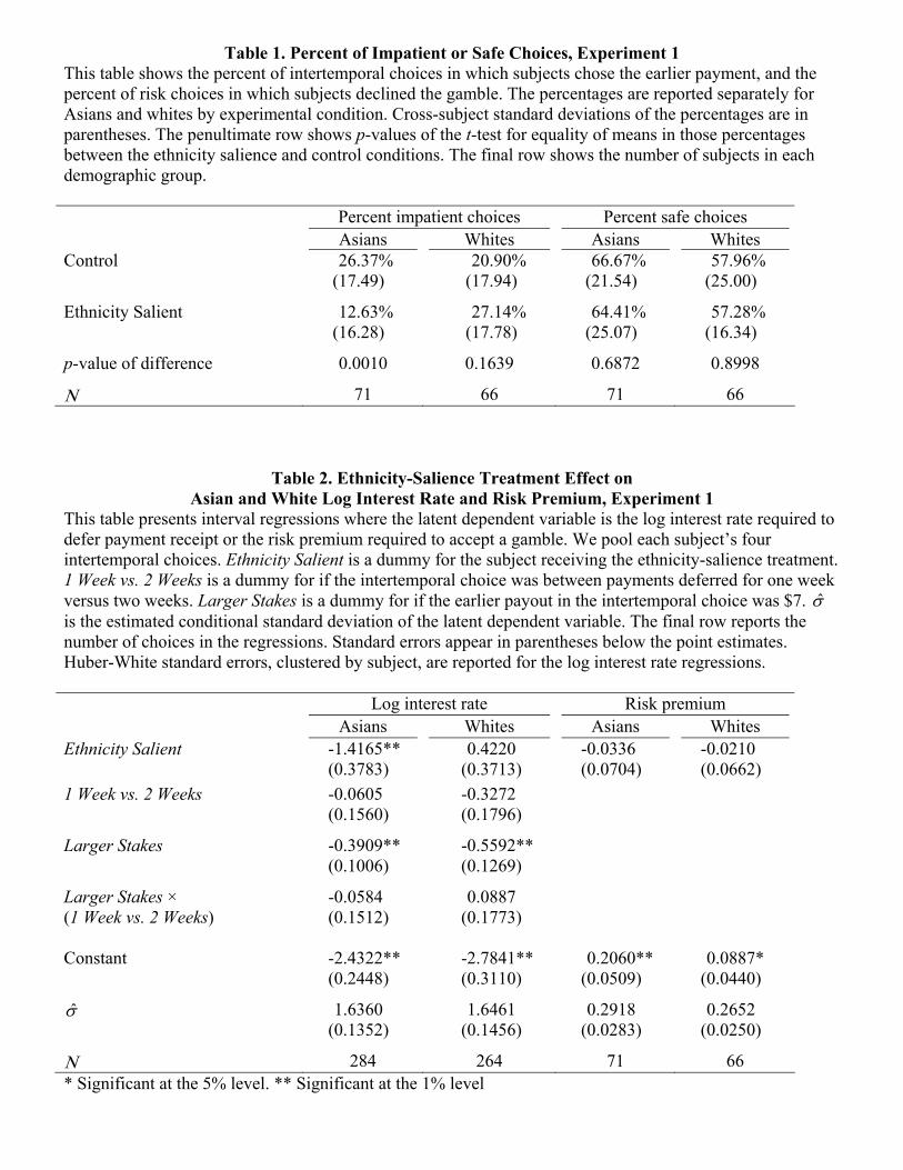
Table 1. Percent of Impatient or Safe Choices, Experiment 1 This table shows the percent of intertemporal choices in which subjects chose the earlier payment, and the percent of risk choices in which subjects declined the gamble. The percentages are reported separately for Asians and whites by experimental condition. Cross-subject standard deviations of the percentages are in parentheses. The penultimate row shows p-values of the t-test for equality of means in those percentages between the ethnicity salience and control conditions. The final row shows the number of subjects in each demographic group.

Percent impatient choices Percent safe choices Asians Whites Asians Whites Control 26.37% 20.90% 66.67% 57.96% (17.49) (17.94) (21.54) (25.00)

Ethnicity Salient 12.63% 27.14% 64.41% 57.28% (16.28) (17.78) (25.07) (16.34)

p-value of difference 0.0010 0.1639 0.6872 0.8998

Ν 71 66 71 66

Table 2. Ethnicity-Salience Treatment Effect on Asian and White Log Interest Rate and Risk Premium, Experiment 1

This table presents interval regressions where the latent dependent variable is the log interest rate required to defer payment receipt or the risk premium required to accept a gamble. We pool each subject’s four intertemporal choices. Ethnicity Salient is a dummy for the subject receiving the ethnicity-salience treatment. 1 Week vs. 2 Weeks is a dummy for if the intertemporal choice was between payments deferred for one week versus two weeks. Larger Stakes is a dummy for if the earlier payout in the intertemporal choice was $7. σ̂ is the estimated conditional standard deviation of the latent dependent variable. The final row reports the number of choices in the regressions. Standard errors appear in parentheses below the point estimates. Huber-White standard errors, clustered by subject, are reported for the log interest rate regressions. Log interest rate Risk premium Asians Whites Asians Whites Ethnicity Salient -1.4165**

(0.3783) 0.4220

(0.3713) -0.0336 (0.0704)

-0.0210 (0.0662)

1 Week vs. 2 Weeks -0.0605 (0.1560)

-0.3272 (0.1796)

Larger Stakes -0.3909** (0.1006)

-0.5592** (0.1269)

Larger Stakes × (1 Week vs. 2 Weeks)

-0.0584 (0.1512)

0.0887 (0.1773)

Constant -2.4322** (0.2448)

-2.7841** (0.3110)

0.2060** (0.0509)

0.0887* (0.0440)

σ̂ 1.6360 (0.1352)

1.6461 (0.1456)

0.2918 (0.0283)

0.2652 (0.0250)

Ν 284 264 71 66 * Significant at the 5% level. ** Significant at the 1% level

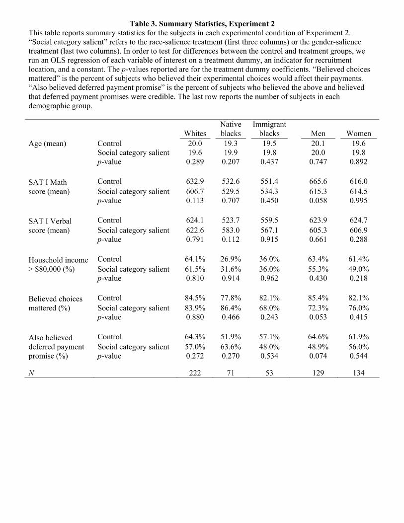
Table 3. Summary Statistics, Experiment 2 This table reports summary statistics for the subjects in each experimental condition of Experiment 2. “Social category salient” refers to the race-salience treatment (first three columns) or the gender-salience treatment (last two columns). In order to test for differences between the control and treatment groups, we run an OLS regression of each variable of interest on a treatment dummy, an indicator for recruitment location, and a constant. The p-values reported are for the treatment dummy coefficients. “Believed choices mattered” is the percent of subjects who believed their experimental choices would affect their payments. “Also believed deferred payment promise” is the percent of subjects who believed the above and believed that deferred payment promises were credible. The last row reports the number of subjects in each demographic group.

Whites Native blacks

Immigrant blacks Men Women

Age (mean) Control 20.0 19.3 19.5 20.1 19.6 Social category salient 19.6 19.9 19.8 20.0 19.8 p-value 0.289 0.207 0.437 0.747 0.892

SAT I Math Control 632.9 532.6 551.4 665.6 616.0 score (mean) Social category salient 606.7 529.5 534.3 615.3 614.5 p-value 0.113 0.707 0.450 0.058 0.995

SAT I Verbal Control 624.1 523.7 559.5 623.9 624.7 score (mean) Social category salient 622.6 583.0 567.1 605.3 606.9 p-value 0.791 0.112 0.915 0.661 0.288

Household income Control 64.1% 26.9% 36.0% 63.4% 61.4% > $80,000 (%) Social category salient 61.5% 31.6% 36.0% 55.3% 49.0% p-value 0.810 0.914 0.962 0.430 0.218

Believed choices Control 84.5% 77.8% 82.1% 85.4% 82.1% mattered (%) Social category salient 83.9% 86.4% 68.0% 72.3% 76.0% p-value 0.880 0.466 0.243 0.053 0.415

Also believed Control 64.3% 51.9% 57.1% 64.6% 61.9% deferred payment Social category salient 57.0% 63.6% 48.0% 48.9% 56.0% promise (%) p-value 0.272 0.270 0.534 0.074 0.544

N 222 71 53 129 134

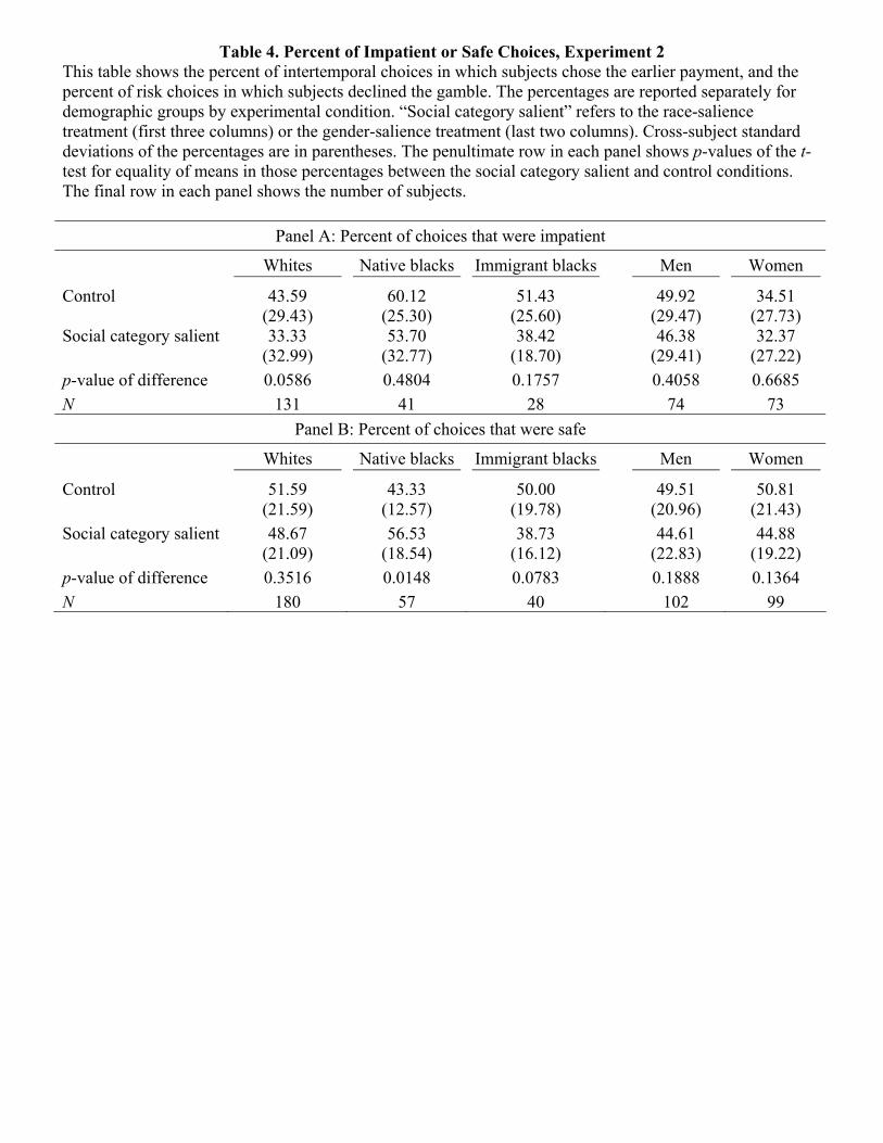
Table 4. Percent of Impatient or Safe Choices, Experiment 2 This table shows the percent of intertemporal choices in which subjects chose the earlier payment, and the percent of risk choices in which subjects declined the gamble. The percentages are reported separately for demographic groups by experimental condition. “Social category salient” refers to the race-salience treatment (first three columns) or the gender-salience treatment (last two columns). Cross-subject standard deviations of the percentages are in parentheses. The penultimate row in each panel shows p-values of the t-test for equality of means in those percentages between the social category salient and control conditions. The final row in each panel shows the number of subjects.

Panel A: Percent of choices that were impatient Whites Native blacks Immigrant blacks Men Women

Control 43.59 60.12 51.43 49.92 34.51 (29.43) (25.30) (25.60) (29.47) (27.73) Social category salient 33.33 53.70 38.42 46.38 32.37 (32.99) (32.77) (18.70) (29.41) (27.22) p-value of difference 0.0586 0.4804 0.1757 0.4058 0.6685 N 131 41 28 74 73

Panel B: Percent of choices that were safe Whites Native blacks Immigrant blacks Men Women

Control 51.59 43.33 50.00 49.51 50.81 (21.59) (12.57) (19.78) (20.96) (21.43) Social category salient 48.67 56.53 38.73 44.61 44.88 (21.09) (18.54) (16.12) (22.83) (19.22) p-value of difference 0.3516 0.0148 0.0783 0.1888 0.1364 N 180 57 40 102 99

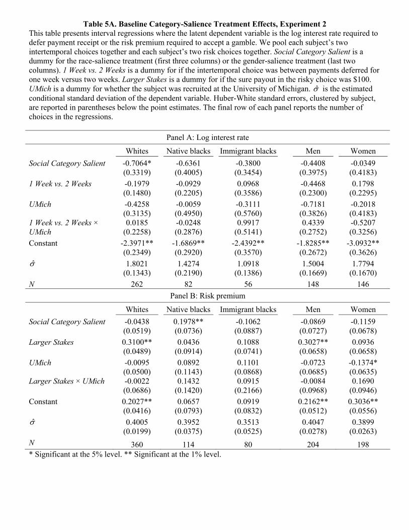
Table 5A. Baseline Category-Salience Treatment Effects, Experiment 2 This table presents interval regressions where the latent dependent variable is the log interest rate required to defer payment receipt or the risk premium required to accept a gamble. We pool each subject’s two intertemporal choices together and each subject’s two risk choices together. Social Category Salient is a dummy for the race-salience treatment (first three columns) or the gender-salience treatment (last two columns). 1 Week vs. 2 Weeks is a dummy for if the intertemporal choice was between payments deferred for one week versus two weeks. Larger Stakes is a dummy for if the sure payout in the risky choice was $100. UMich is a dummy for whether the subject was recruited at the University of Michigan. σ̂ is the estimated conditional standard deviation of the dependent variable. Huber-White standard errors, clustered by subject, are reported in parentheses below the point estimates. The final row of each panel reports the number of choices in the regressions.

Panel A: Log interest rate Whites Native blacks Immigrant blacks Men Women Social Category Salient -0.7064* -0.6361 -0.3800 -0.4408 -0.0349 (0.3319) (0.4005) (0.3454) (0.3975) (0.4183) 1 Week vs. 2 Weeks -0.1979 -0.0929 0.0968 -0.4468 0.1798 (0.1480) (0.2205) (0.3586) (0.2300) (0.2295) UMich -0.4258 -0.0059 -0.3111 -0.7181 -0.2018 (0.3135) (0.4950) (0.5760) (0.3826) (0.4183) 1 Week vs. 2 Weeks × 0.0185 -0.0248 0.9917 0.4339 -0.5207 UMich (0.2258) (0.2876) (0.5141) (0.2752) (0.3256) Constant -2.3971** -1.6869** -2.4392** -1.8285** -3.0932** (0.2349) (0.2920) (0.3570) (0.2672) (0.3626) σ̂ 1.8021 1.4274 1.0918 1.5004 1.7794 (0.1343) (0.2190) (0.1386) (0.1669) (0.1670) N 262 82 56 148 146

Panel B: Risk premium Whites Native blacks Immigrant blacks Men Women Social Category Salient -0.0438 0.1978** -0.1062 -0.0869 -0.1159 (0.0519) (0.0736) (0.0887) (0.0727) (0.0678) Larger Stakes 0.3100** 0.0436 0.1088 0.3027** 0.0936 (0.0489) (0.0914) (0.0741) (0.0658) (0.0658) UMich -0.0095 0.0892 0.1101 -0.0723 -0.1374* (0.0500) (0.1143) (0.0868) (0.0685) (0.0635) Larger Stakes × UMich -0.0022 0.1432 0.0915 -0.0084 0.1690 (0.0686) (0.1420) (0.2166) (0.0968) (0.0946) Constant 0.2027** 0.0657 0.0919 0.2162** 0.3036** (0.0416) (0.0793) (0.0832) (0.0512) (0.0556) σ̂ 0.4005 0.3952 0.3513 0.4047 0.3899 (0.0199) (0.0375) (0.0525) (0.0278) (0.0263) N 360 114 80 204 198 * Significant at the 5% level. ** Significant at the 1% level.

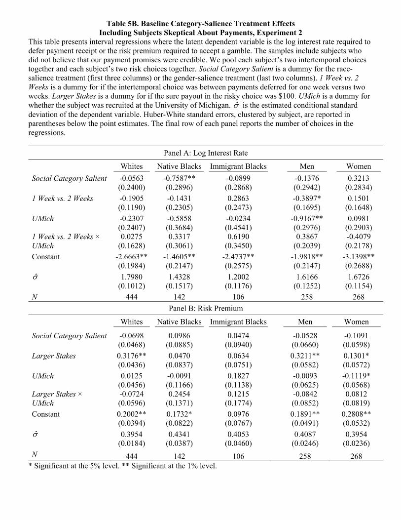
Table 5B. Baseline Category-Salience Treatment Effects Including Subjects Skeptical About Payments, Experiment 2

This table presents interval regressions where the latent dependent variable is the log interest rate required to defer payment receipt or the risk premium required to accept a gamble. The samples include subjects who did not believe that our payment promises were credible. We pool each subject’s two intertemporal choices together and each subject’s two risk choices together. Social Category Salient is a dummy for the race-salience treatment (first three columns) or the gender-salience treatment (last two columns). 1 Week vs. 2 Weeks is a dummy for if the intertemporal choice was between payments deferred for one week versus two weeks. Larger Stakes is a dummy for if the sure payout in the risky choice was $100. UMich is a dummy for whether the subject was recruited at the University of Michigan. σ̂ is the estimated conditional standard deviation of the dependent variable. Huber-White standard errors, clustered by subject, are reported in parentheses below the point estimates. The final row of each panel reports the number of choices in the regressions.

Panel A: Log Interest Rate Whites Native Blacks Immigrant Blacks Men Women Social Category Salient -0.0563 -0.7587** -0.0899 -0.1376 0.3213 (0.2400) (0.2896) (0.2868) (0.2942) (0.2834) 1 Week vs. 2 Weeks -0.1905 -0.1431 0.2863 -0.3897* 0.1501 (0.1190) (0.2305) (0.2473) (0.1695) (0.1648) UMich -0.2307 -0.5858 -0.0234 -0.9167** 0.0981 (0.2407) (0.3684) (0.4541) (0.2976) (0.2903) 1 Week vs. 2 Weeks × 0.0275 0.3317 0.6190 0.3867 -0.4079 UMich (0.1628) (0.3061) (0.3450) (0.2039) (0.2178) Constant -2.6663** -1.4605** -2.4737** -1.9818** -3.1398** (0.1984) (0.2147) (0.2575) (0.2147) (0.2688) σ̂ 1.7980 1.4328 1.2002 1.6166 1.6726 (0.1012) (0.1517) (0.1176) (0.1252) (0.1154) N 444 142 106 258 268

Panel B: Risk Premium Whites Native Blacks Immigrant Blacks Men Women

Social Category Salient -0.0698 0.0986 0.0474 -0.0528 -0.1091 (0.0468) (0.0885) (0.0940) (0.0660) (0.0598) Larger Stakes 0.3176** 0.0470 0.0634 0.3211** 0.1301* (0.0436) (0.0837) (0.0751) (0.0582) (0.0572) UMich 0.0125 -0.0091 0.1827 -0.0093 -0.1119* (0.0456) (0.1166) (0.1138) (0.0625) (0.0568) Larger Stakes × -0.0724 0.2454 0.1215 -0.0842 0.0812 UMich (0.0596) (0.1371) (0.1774) (0.0852) (0.0819) Constant 0.2002** 0.1732* 0.0976 0.1891** 0.2808** (0.0394) (0.0822) (0.0767) (0.0491) (0.0532) σ̂ 0.3954 0.4341 0.4053 0.4087 0.3954 (0.0184) (0.0387) (0.0460) (0.0246) (0.0236) N 444 142 106 258 268

* Significant at the 5% level. ** Significant at the 1% level.

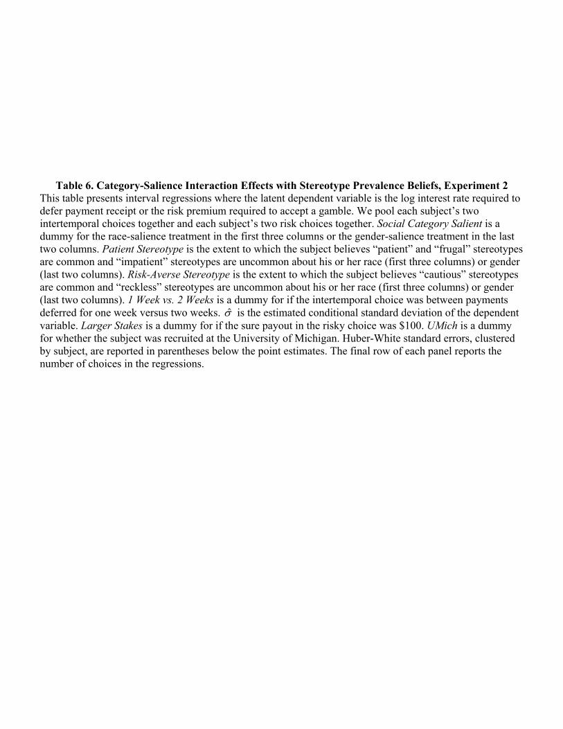
Table 6. Category-Salience Interaction Effects with Stereotype Prevalence Beliefs, Experiment 2 This table presents interval regressions where the latent dependent variable is the log interest rate required to defer payment receipt or the risk premium required to accept a gamble. We pool each subject’s two intertemporal choices together and each subject’s two risk choices together. Social Category Salient is a dummy for the race-salience treatment in the first three columns or the gender-salience treatment in the last two columns. Patient Stereotype is the extent to which the subject believes “patient” and “frugal” stereotypes are common and “impatient” stereotypes are uncommon about his or her race (first three columns) or gender (last two columns). Risk-Averse Stereotype is the extent to which the subject believes “cautious” stereotypes are common and “reckless” stereotypes are uncommon about his or her race (first three columns) or gender (last two columns). 1 Week vs. 2 Weeks is a dummy for if the intertemporal choice was between payments deferred for one week versus two weeks. σ̂ is the estimated conditional standard deviation of the dependent variable. Larger Stakes is a dummy for if the sure payout in the risky choice was $100. UMich is a dummy for whether the subject was recruited at the University of Michigan. Huber-White standard errors, clustered by subject, are reported in parentheses below the point estimates. The final row of each panel reports the number of choices in the regressions.

Panel A: Log interest rate

Whites Native blacks Immigrant blacks Men Women Social Category Salient -0.6991* -0.5749 -0.4494 -0.3682 -0.1519 (0.3334) (0.3474) (0.3327) (0.4130) (0.4571) Social Category Salient 0.0962 0.7477* -0.0758 0.2339 -0.2951 × Patient Stereotype (0.3525) (0.3108) (0.3332) (0.3738) (0.4364) Patient Stereotype -0.0419 -0.4575** 0.0573 -0.0556 0.1792 (0.2488) (0.1604) (0.2507) (0.3004) (0.2647) 1 Week vs. 2 Weeks -0.1982 -0.0949 0.0963 -0.4504 0.1799 (0.1482) (0.2180) (0.3599) (0.2337) (0.2272) UMich -0.4361 0.2410 -0.0105 -0.8419 -0.0696 (0.3196) (0.4920) (0.6298) (0.4835) (0.4428) 1 Week vs. 2 Weeks 0.0115 0.1193 0.9008 0.3159 -0.5019 × UMich (0.2291) (0.2596) (0.5968) (0.3008) (0.3084) Constant -2.4022** -1.7327** -2.4105** -1.8453** -3.0378** (0.2362) (0.2487) (0.3587) (0.3133) (0.3716) σ̂ 1.8087 1.2905 1.1063 1.5345 1.7356 (0.1354) 0.2226 (0.1548) (0.1863) (0.1798) N 260 76 52 122 120

Panel B: Risk premium Whites Native blacks Immigrant blacks Men Women Social Category Salient -0.0468 0.2378** -0.1284 -0.0861 -0.1232 (0.0526) (0.0860) (0.0957) (0.0727) (0.0696) Social Category Salient -0.0132 -0.0907 -0.0316 0.1611* 0.1243 × Risk-Averse Stereotype (0.0560) (0.0942) (0.1296) (0.0817) (0.0882) Risk-Averse Stereotype 0.0253 -0.0010 0.0482 -0.0522 -0.0023 (0.0354) (0.0547) (0.1144) (0.0569) (0.0725) Larger Stakes 0.3104** 0.0333 0.1087 0.3000** 0.0940 (0.0491) (0.0982) (0.0746) (0.0658) (0.0661) UMich -0.0049 0.1634 0.0755 -0.0082 -0.1675* (0.0504) (0.1387) (0.1015) (0.0851) (0.0765) Larger Stakes × UMich -0.0012 0.1505 0.2394 -0.1115 0.1954 (0.0692) (0.1765) (0.2489) (0.0870) (0.1182) Constant 0.2021** 0.0383 0.1066 0.2110** 0.3104** (0.0413) (0.0848) (0.0918) (0.0515) (0.0596) σ̂ 0.4006 0.4197 0.3526 0.3853 0.3863 (0.0198) (0.0393) (0.0516) (0.0270) (0.0295) N 358 98 76 170 162 * Significant at the 5% level. ** Significant at the 1% level.

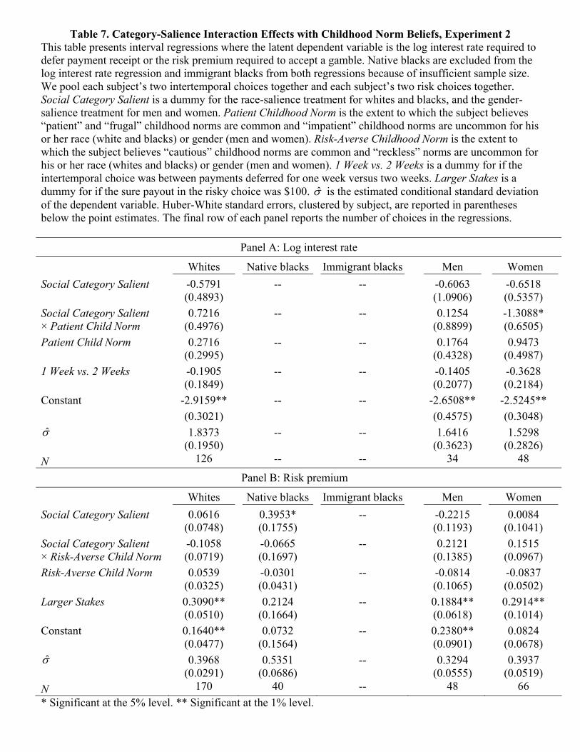
Table 7. Category-Salience Interaction Effects with Childhood Norm Beliefs, Experiment 2 This table presents interval regressions where the latent dependent variable is the log interest rate required to defer payment receipt or the risk premium required to accept a gamble. Native blacks are excluded from the log interest rate regression and immigrant blacks from both regressions because of insufficient sample size. We pool each subject’s two intertemporal choices together and each subject’s two risk choices together. Social Category Salient is a dummy for the race-salience treatment for whites and blacks, and the gender-salience treatment for men and women. Patient Childhood Norm is the extent to which the subject believes “patient” and “frugal” childhood norms are common and “impatient” childhood norms are uncommon for his or her race (white and blacks) or gender (men and women). Risk-Averse Childhood Norm is the extent to which the subject believes “cautious” childhood norms are common and “reckless” norms are uncommon for his or her race (whites and blacks) or gender (men and women). 1 Week vs. 2 Weeks is a dummy for if the intertemporal choice was between payments deferred for one week versus two weeks. Larger Stakes is a dummy for if the sure payout in the risky choice was $100. σ̂ is the estimated conditional standard deviation of the dependent variable. Huber-White standard errors, clustered by subject, are reported in parentheses below the point estimates. The final row of each panel reports the number of choices in the regressions.

Panel A: Log interest rate Whites Native blacks Immigrant blacks Men Women Social Category Salient -0.5791 -- -- -0.6063 -0.6518 (0.4893) (1.0906) (0.5357) Social Category Salient 0.7216 -- -- 0.1254 -1.3088* × Patient Child Norm (0.4976) (0.8899) (0.6505) Patient Child Norm 0.2716 -- -- 0.1764 0.9473 (0.2995) (0.4328) (0.4987) 1 Week vs. 2 Weeks -0.1905 -- -- -0.1405 -0.3628 (0.1849) (0.2077) (0.2184) Constant -2.9159** -- -- -2.6508** -2.5245** (0.3021) (0.4575) (0.3048) σ̂ 1.8373 -- -- 1.6416 1.5298 (0.1950) (0.3623) (0.2826) N 126 -- -- 34 48

Panel B: Risk premium Whites Native blacks Immigrant blacks Men Women Social Category Salient 0.0616 0.3953* -- -0.2215 0.0084 (0.0748) (0.1755) (0.1193) (0.1041) Social Category Salient -0.1058 -0.0665 -- 0.2121 0.1515 × Risk-Averse Child Norm (0.0719) (0.1697) (0.1385) (0.0967) Risk-Averse Child Norm 0.0539 -0.0301 -- -0.0814 -0.0837 (0.0325) (0.0431) (0.1065) (0.0502) Larger Stakes 0.3090** 0.2124 -- 0.1884** 0.2914** (0.0510) (0.1664) (0.0618) (0.1014) Constant 0.1640** 0.0732 -- 0.2380** 0.0824 (0.0477) (0.1564) (0.0901) (0.0678) σ̂ 0.3968 0.5351 -- 0.3294 0.3937 (0.0291) (0.0686) (0.0555) (0.0519) N 170 40 -- 48 66 * Significant at the 5% level. ** Significant at the 1% level.

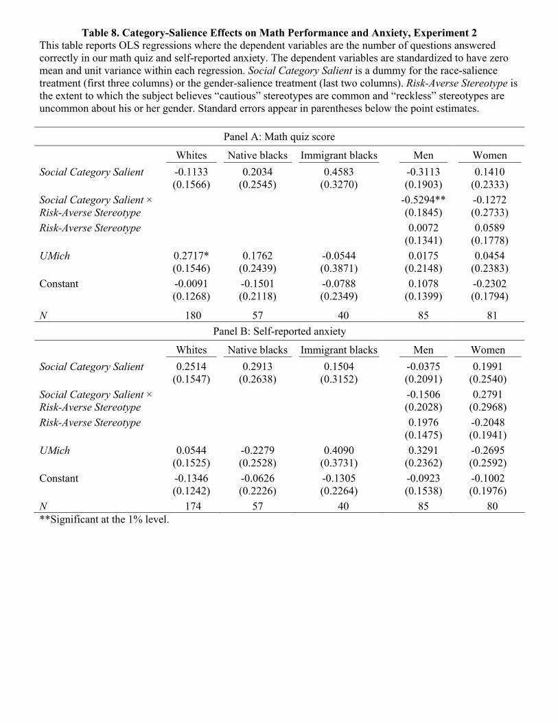
Table 8. Category-Salience Effects on Math Performance and Anxiety, Experiment 2 This table reports OLS regressions where the dependent variables are the number of questions answered correctly in our math quiz and self-reported anxiety. The dependent variables are standardized to have zero mean and unit variance within each regression. Social Category Salient is a dummy for the race-salience treatment (first three columns) or the gender-salience treatment (last two columns). Risk-Averse Stereotype is the extent to which the subject believes “cautious” stereotypes are common and “reckless” stereotypes are uncommon about his or her gender. Standard errors appear in parentheses below the point estimates. Panel A: Math quiz score Whites Native blacks Immigrant blacks Men Women Social Category Salient -0.1133 0.2034 0.4583 -0.3113 0.1410 (0.1566) (0.2545) (0.3270) (0.1903) (0.2333) Social Category Salient × -0.5294** -0.1272 Risk-Averse Stereotype (0.1845) (0.2733) Risk-Averse Stereotype 0.0072 0.0589 (0.1341) (0.1778) UMich 0.2717* 0.1762 -0.0544 0.0175 0.0454 (0.1546) (0.2439) (0.3871) (0.2148) (0.2383) Constant -0.0091 -0.1501 -0.0788 0.1078 -0.2302 (0.1268) (0.2118) (0.2349) (0.1399) (0.1794)

N 180 57 40 85 81 Panel B: Self-reported anxiety

Whites Native blacks Immigrant blacks Men Women Social Category Salient 0.2514 0.2913 0.1504 -0.0375 0.1991 (0.1547) (0.2638) (0.3152) (0.2091) (0.2540) Social Category Salient × -0.1506 0.2791 Risk-Averse Stereotype (0.2028) (0.2968) Risk-Averse Stereotype 0.1976 -0.2048 (0.1475) (0.1941) UMich 0.0544 -0.2279 0.4090 0.3291 -0.2695 (0.1525) (0.2528) (0.3731) (0.2362) (0.2592) Constant -0.1346 -0.0626 -0.1305 -0.0923 -0.1002 (0.1242) (0.2226) (0.2264) (0.1538) (0.1976) N 174 57 40 85 80 **Significant at the 1% level.