DRAFT: May 1999

REVISED: July 1999

SECOND REVISION: August 1999

SOCIAL SECURITY REFORMand

LABOR MARKETS: THE CASE OF CHILE*

By

SEBASTIAN EDWARDSUniversity of California, Los Angeles

andNational Bureau of Economic Research

And

ALEJANDRA COX EDWARDSCalifornia State University, Long Beach

ABSTRACT

In 1981, Chile reformed its social security system. An inefficient and insolvent pay-as-you-go regime was replaced by system based on individual retirement accounts. Overthe years Chile’s reform has been widely praised, and has been carefully studied bypolicy makers throughout the world. In this paper we focus on a neglected aspect ofChile’s social security reform: its impact on labor market outcomes, includingunemployment and wages. We develop a model of the labor market where we assumethat, as is the case in most emerging markets, a formal and an informal sectors coexistside by side. According to our model, a social security reform that reduces the implicittax on labor in the formal sector, will result in an increase in the wage rate in the informalsector and will have an undetermined effect on aggregate unemployment. Results fromsimulation exercises suggest that in the case of Chile the reforms resulted in an increasein informal sector wages between 2 an 2.5%. These results also suggest that the reformsmade a positive contribution to the reduction of Chile’s aggregate of unemployment.

____________________* We are indebted to Manuelita Ureta for helpful discussions, and to Alejandro Jara andRajesh Chakrabarti for assistance.

1

I. Introduction

In recent years policy makers, politicians and academics have become deeply

concerned about the future of social security. The specter of a massive insolvency crisis

has generated, through out the world, a frantic search for a solution to what the World

Bank (1994) has called the “old age crisis.” Conferences have been organized, wise-men

groups have been assembled, and blueprints for reform have been discussed. Throughout

this process, and in an effort to learn from lessons of experience, many analysts have

focused on Chile’s pioneering social security reform. In 1980 Chile replaced an insolvent

and highly inefficient government-run social security system, by a privately managed

system based on individual retirement accounts. Almost twenty years after the launching

of this privatization effort, the Chilean experience has become a required case study for

anyone interested in reforming social security.1 Most analyses of Chile’s experience

have concentrated on three aspects of this privatization program: (1) Its effect on the

fiscal accounts, including its effect on public sector’s contingent liabilities. (2) The

effects of the new system on old-age pensions, including a comparison of replacement

rates under the old a new regime. And (3) the effects of the reform on aggregate national

savings.2

Surprisingly, very few studies of the Chilean episode have dealt with the overall

labor market implications of the social security reforms. This, however, is not unique of

the Chilean case. In fact, while a number of studies for a variety of countries have

analyzed the way in which social security systems affect labor market incentives for older

individuals, very few authors have analyzed formally the way in which a major social

security reform affects overall labor market outcomes.3 And yet, it may be argued that a

reform that (in principle) changes the rate of payroll taxes, and affects the relationship

between social security contributions and future earnings will have substantial effects on

the aggregate and (sectoral) demand and supply for labor. This would be clearly the case

if contributions to the pay-as-you go system are considered (at least in part) a tax, and

1 On Chile’s reforms, see Edwards and Edwards (1991) and Bosworth, Dornbush and Laban (1994).2 See, for example, the discussion in Diamond and Valdes-Prieto (1994).3 The papers collected in Grueber and Wise (1999) analyze in great detail the way in social security affectslabor force decisions of older persons in eleven industrialized countries.

2

contributions to individual retirement accounts are seen largely as deferred

compensation.4

The privatization of social security – either partially or fully – is likely to have a

particularly significant effect on overall labor markets outcomes in emerging economies,

including in former socialist nations. Most emerging countries are characterized by

segmented labor markets, where a modern and an informal labor market coexist. Under

these circumstances, only those employed in the “modern” segment will be covered by

labor market regulations, including social security. Those employed in the so-called

informal sector work without formal contracts, generally don’t pay taxes, are not affected

by minimum wages laws, and are excluded from the formal safety net.

The purpose of this paper is to analyze the way in which a social security reform

of the Chilean-type affects labor market outcomes in an economy characterized by a

segmented labor market. Our main interest is to evaluate the way in which Chile’s social

security reform affected the country’s level of employment, its rate of unemployment and

wages in different sectors. In order to do this we develop a model of the labor market in

an emerging economy, and we simulate it using parameter values for Chile. We also use

micro survey data to investigate some key features, such as coverage, of Chile’s

privatized social security system. The paper is organized as follows: Section I is the

introduction. In Section II we provide a brief evaluation of Chile’s social security

reform. Section III deals with the effects of social security reform on wages, income

distribution, employment and unemployment. The section begins with a general

discussion of Chile’s labor market reforms. We next develop a model of a segmented

labor market to analyze the way in which policies aimed at reducing the tax component

of social security contribution affect the key labor market variables. In section IV we

analyze empirically the case of Chile. We first use micro survey data to analyze the

extent of coverage of the new privatized system. We also use these data to analyze

whether, as expected by the architects of the reforms, individual participants consider

contributions into the new system as deferred compensation. In Section V we calibrate

the model, using parameters that capture Chile’s economic structure, and we simulate the

4 Siebert (1998), Lorz (1998) and Edwards (1998b) constitute some of the few papers that analyze thepossible effects of social security reforms on labor markets.

3

way in which a social security reform that lowers the pay roll tax affects labor market

outcomes. The results from our simulation exercise suggest that the effect of the reform

on Chile’s aggregate employment was rather modest. The results also suggest that the

reforms resulted in an increase in average wages. Finally, in section VI we provide some

concluding remarks.

II. The Privatization of Chile’s Social Security System

In late 1980 Chile’s military regime, led by General Augusto Pinochet, privatized

the country’s traditional pay-as-you-go social security system. The decision to replace

the government-run program by one based on privately managed individual retirement

accounts was part of an ambitious program aimed at transforming Chile into a market-

oriented economy. Almost twenty years after Chile’s social security reform, most

observers agree that Chile’s program was a true pioneer, and that there is much to learn

from it. In this section we provide a brief discussion of the main aspects of the reform.

Readers interested in greater detail are referred to Diamond and Valdes-Prieto (1994),

and Edwards (1998a, b).

II.1 The Old Pay-as-you-go System

Chile’s original social security system was adopted in the 1920s, and was

supposed to work as a collective capitalization fund. Accumulated funds, however, were

poorly managed, and benefits -- especially for the better to do -- escalated quickly. For all

practical purposes, and in spite of the original intentions of its founders, by the 1970s the

system had become an insolvent pay-as-you-go regime, characterized by very high

contribution rates. In 1973, for example, total contributions to the retirement plan -- by

employers and employees -- averaged 26 percent of wages. Once contributions to the

national health system were included, total contributions exceeded, for some workers, 50

percent of wages. What made things worse was that there was almost no connection

between retirement contributions and (perceived) benefits. Contributions were largely

seen as taxes, while benefits received from the social security system were seen as

entitlements (Cox Edwards 1992, Diamond and Valdes-Prieto 1994).

While in 1955 there were 12 active contributors per retiree, by 1979 there were

only 2.5. As a result of this, and of a highly inefficient management, the Chilean system

4

became increasingly unfunded. By the early 1970s the system as a whole was already

running a dramatic deficit. The gap between revenues and outlays -- administrative costs

plus pensions -- was made up by the public sector. By 1971 the central government’s

contributions to the retirement system amounted to almost 3% of GDP, and the present

valued of the system’s contingent liabilities exceeded 100% of GDP.

II.2 The Privatization of Social Security in Chile

In 1980 the military government decided to introduce a sweeping reform to the

retirement system. In an effort to increase the attractiveness of the new system, and in

order to reduce political opposition, contribution rates under the new system were

lowered; as a result, those individuals that joined the new system experienced an average

increase of net take-home pay equal to10% (Iglesias and Vittas, 1992). It was expected

that, given the anticipated higher rates of return on the accumulated funds, the lower

contributions would be enough to finance higher replacement rates for pensions.

The core of Chile’s new system are individual retirement accounts managed by

private companies known as “Administradoras de Fondos de Pensiones”, AFPs. Each

AFP can manage only one retirement fund; likewise, each participant can have only one

retirement account. A key feature of the system is that it is mandatory for individuals

working for a formal employee. Participants can freely decide which AFP will manage

their retirement funds, and are free to transfer their funds across the different

management firms. On retirement, individuals can choose to buy an annuity, or to

withdraw their funds according to a predetermined (actuarially fair) plan. The system

also has a survivor’s term life insurance component, and a disability program funded with

an additional insurance premium. In the reformed system, the State continues to play an

important role. It regulates and monitors the operation of the management companies,

and guarantees “solidarity in the base” through a minimum pension5.

Contributions to the retirement component of the system are equal to 10% of

income, considerably lower then the 26% (on average) under the old system. Total

contributions for retirement, health and survivorship insurance add up to 20% of wages,

with a cap equivalent to an annual wage rate of US$40,000 per year. A detailed

5 In case an accumulated fund does not provide for an annuity above the minimum pension, the statecomplements the funds, so long as the individual has made contributions for a minimum of twenty years.

5

regulatory framework -- enforced by an institution especially created for this purpose, the

Superintendency of AFPs -- regulates investment portfolios, ensures free determination

of fees and commissions and free entry into the industry.

Self employed workers are not required to participate in the system. They have

the choice, however, to set retirement accounts which are (basically) subject to the same

regulations as those of formal sector employees. In 1998 the percentage of active

contributors – that is those making deposits into their retirement accounts --stood at 58%

of total employment; in addition 4% of workers were still affected by the old system.

This means, then, that in 1998 the total coverage of the Chilean retirement system

amounted to 62% of employment. The 38% that is not covered by the social security

system corresponds, largely, to those that work in the informal sector, or to the self

employed (for details on the actual characteristics of those not covered by the new

system, see the discussion in section III of this paper). At 62% of employment, the

current coverage of the system is similar to that of the old pay-as-you-go system. The

lack of universal coverage represents an important weakness of the privatization scheme,

and is explained by two basic factors: first, the self-employed – which are not legally

required to participate in the system-- have very little incentives to make voluntary

contributions. Second, the existence of a government-guaranteed (universal) minimum

pension creates a moral hazard situation among low income workers, many of which are

self employed. For these individuals it pays to contribute only sporadically, and only

enough as to obtain the minimum pension once they retire.6

The volume of pension funds privately managed by the AFPs has increased

dramatically. Between 1985 and 1997 they increased from 10% of GDP to almost 45%

of GDP. Furthermore, recent simulations suggest that by year 2010 the accumulated

funds will represent 110% of GDP, and that by 2020 they would have reached 134% of

GDP (Fuentes, 1995). The type of assets the retirement funds can invest in are tightly

regulated. During the early years, funds were largely restricted to government securities,

bank deposits, investment grade corporate bonds and mortgage bonds. At this time,

however, a number of equities, both domestic and foreign, are allowed.

6 See Edwards (1998a) for details on the system’s operative aspects.

6

During the early years of the reform the real (inflation adjusted) average rate of

return of accumulated funds was very high, averaging during 1982-1995, 12.8 percent per

annum. More recently, however, the rate of return has declined significantly, and has

averaged, between 1995 and 1997, 1.9%. Existing regulations impose a floor on the

return individual AFP pay to their members. In any given year an AFP cannot pay a

return lower than 2 percentage points of the system’s average. If the actual return of a

particular AFP falls below this minimum, the difference has to be made up by using

funds from a specially set “reserve fund.” The restriction on a minimum rate of return,

coupled with the regulations that each AFP cannot have more than one fund, and that

individuals cannot distribute their funds across funds, has reduced the extent of

competition of the system, and has resulted in the different AFPs holding extremely

similar portfolios.

The new system allows men to retire at 65, and women at 60, or earlier if they

have accumulated enough funds to finance a pension of 70 percent of their (pensionable)

salary. When an individual retires he can choose between two systems: (A) he can use

the accumulated funds to buy an annuity from an insurance company; or, (B) he can

chose to enroll in a “programmed withdrawal” scheme, where the accumulated funs are

drawn according to an actuarially determined schedule. By 1997 there were already

250,000 retirees receiving pensions under the new system. Of these, approximately one

half had opted for annuities, and one half for programmed withdrawal. Using a sample of

4,064 individuals that have retired under the new system Baeza and Burger (1995)

estimated that the average replacement rate had amounted to 78%, significantly higher

than under the old pay-as-you-go regime.

The new system also establishes that, for those individuals that qualify, there is a

minimum pension guaranteed by the state, which as of December 1998 was equal to 85%

of the minimum wage. From an international comparative perspective, replacement rates

have been quite high in Chile – indeed higher than under most industrialized countries’

systems.7

7 On industrial countries replacement rates see, for example, Davis (1998) and the papers in Grueber andWise (1999). Naturally, since this is a defined contribution system, future replacement rates may vary.

7

II.3 The Transition from the Pay-as-you-go to the Privatized System

Most proposals to privatize social security, struggle with issues related to the

transition. Chile dealt with this problem in a simple, and yet effective manner. All

transitional costs were borne by the government and were paid out of the general budget.

Individuals that had been contributing to the old system received government bonds – the

so-called “recognition bonds”. These bonds yielded per annum 4% in inflation adjusted

terms, an were placed in the each individual retirement account. The value of the bonds

received by each person was determined using a formula that took into account their

history of contributions to the old system. From a fiscal point of view the transition was

rather expensive, representing almost 5%of GDP in the peak year of 1983. It is estimated

that by 2015 these costs would have almost disappeared (Edwards 1998a).

II.4 Chile’s Social Security and Labor Market Reforms

The reform of social security was only one component of a broad effort to

transform Chile into a modern market economy. During the second half of the 1970s the

military government implemented a number of fundamental reforms, including a major

overhaul of the tax system, the opening up of the economy to international competition,

the privatization of most state owned enterprises, and the creation of a modern financial

market. In the early 1980’s the scope of the reforms was broadened to include labor

markets and social security.

In 1979, and under considerable international pressure, the military government

initiated an effort to reform Chile’s labor legislation. The main objectives of these

policies were: (a) To reform job security legislation, by limiting the extent of severance

payments. These were reduced form “one month per year of service, with no limit”, to

“one month per year of service, with a 5 months limit.” (b) To reduce unions’ power by

decentralizing collective bargaining, and eliminating the old “close-shop” practice. And

(c), reduce payroll taxes. This last measure was to be achieved, partially, by the social

security reform, discussed above.8

Between 1985 and 1997, Chile’s labor markets performed remarkably well.9

What makes this experience particularly interesting is that between 1983-85 and 1993-95,

8 See Edwards and Edwards (1999) for details on the labor reforms.9 Strictly speaking this improved performance began in 1985-86, after Chile recovered from the debt crisis.

8

Chile went from rates of unemployment usually associated with some European

countries, to unemployment rates similar to those traditionally prevailing in the U.S.

While during 1983-85 the open rate of unemployment averaged 17.3%, by 1993-95 it had

declined to 5.8 percent. And all of this while real wages experienced rates of growth in

excess of 5% per year.10 An interesting question is which of the components of the labor-

related reforms – the reduced degree of job security, the reformed collective bargaining,

or the social security reform -- were more important in helping Chile improve its labor

market performance. Although providing a full answer to this question is beyond the

scope of this paper, in section III we develop a model that allow us to quantify the effect

of the social security reform on some of the key labor market variables. We proceed as

follows: we first develop (in Section III) a model of segmented labor market, and

investigate the way in which changes in taxes on labor in the “covered or modern” sector

impact labor market outcomes. Next, in Section IV, we use micro survey data to analyze

the extent to which participants truly considered the new system as a “deferred

compensation” scheme. Finally, in Section V, we calibrate and simulate the model for

the case of Chile. Our findings suggest that the social security reform had a modest

effect on Chile’s labor market performance. This, however, needs not be the case in

other countries: the actual impact of a Chile-style social security reform on

unemployment, wages and income distribution will depend on the specific values of the

relevant parameters.

IV. A Model of Social Security Reform and Labor Markets

Labor markets in emerging economies in general – and in Chile, in particular –,

have a number of institutional features that set them apart from labor markets in industrial

nations. The most important among these features are:

• In emerging countries labor markets are usually characterized by a rather large

“informal” segment. This segment is, de facto, not directly affected by labor market

regulations, such as minimum wages, job security legislation or social security. The

informal sector coexists with a “modern” sector, where labor market regulations are

fully in effect. The fact that in Chile the social security system covers only 62% of 10 The initial level of wages was, however, highly depressed (Edwards and Edwards, 1991).

9

those employed, provides some evidence of the existence of this segmented structure.

Moreover, Basch and Paredes (1996) present micro-based evidence for Chile that

supports the view that the country’s labor market is characterized by the coexistence

of these two labor segments.

• Contributions to social security are often seen as a (partial) tax on labor, rather than as

deferred compensation, or an insurance program. At the same time, benefits from

these programs are seen by individuals as an entitlement (Cox Edwards 1992). The

percentage of the contribution that is actually considered a pure tax depends on the

nature of the social security system and, more specifically, on the perceived

connection between contributions and benefits (Diamond and Valdes-Prieto 1994).

In the case of Chile, Torche and Wagner (1997) have argued that, although the reform

reduced the tax component of contributions to social security, it did not fully

eliminated it. In section III of this paper we use micro survey data to investigate this

issue in detail.

Formally, assume that, as is the case in many developing and transitional

economies, the labor market is segmented. There is a “modern” or “covered” sector

subject to a minimum wage and to social security coverage, and an “informal” or

“unprotected” sector with no social security coverage, and competitively determined

wages. With other things equal, workers will rather be employed in the “protected”

sector. The problem, however, is that there are not enough jobs in that sector; individuals

that apply for a job in the modern sector face a probability (p) of obtaining it, and a

probability (1-p) of being unemployed. In equilibrium, and under the assumption of risk

neutrality, the wage rate obtained in the informal segment is equal to the expected (take

home) wage rate in the protected sector. We further assume that every period

employment in the modern sector turns over fully, so that the probability of getting a job

there is equal to the ratio of openings to applicants.11

We also assume that prior to the reform workers in the protected sector are

subject to a payroll tax – whose purpose is to fund the social security system—equal to

T1. We also assume that there is a disconnect between social security contributions and 11 This mechanism is similar to the one consider in migration models of the Harris-Todaro type. In ourmodel, however, there is no migration. The assumption of risk neutrality is not essential; all the resultswill follow if individuals have a constant degree of risk aversion.

10

benefits. More specifically, we assume that social security contributions are considered

by individuals to be fully a tax. Notice, however, that the analysis that follows would not

be affected by the assumption that only a fraction of the contribution was considered to

be a tax. Workers employed in the modern sector receive a “take home” wage rate equal

to the minimum wage (Wmin ). The cost of labor to firms operating in this sector is equal

to minimum wage rate plus the payroll tax. The social security reform will result in a

reduction of this tax. There are two sources for this reduction: first, as was the case in

Chile, the reform itself may entail a reduction in the contribution. Second, the

replacement of the old pay-as-you-go system by individual retirement accounts, reduces

the disconnect between contributions and benefits. In the post reform period, at least part

of the contribution will be considered as deferred compensation (see Section IV for an

estimate.)

Equations (1) - (4) describe the wage determination process in this economy.

Equation (1) establishes that in equilibrium the wage rate in the informal sector (WI) is

equal to the expected (net of taxes) wage rate in the modern sector E (W N M). According

to equation (2) the probability of finding a job in the modern sector is equal to the ratio of

openings – that is employment in that sector (L M) – to applicants. The latter is given by

the sum of openings plus the total number of unemployed (L M + U). It is assumed, for

simplicity, that the unemployed received an income equal to S. Equation (3) says that the

cost of labor in the modern sector is equal to the minimum wage inclusive of the payroll

tax ( T1). In equation (4) we present the demand for labor equations in the modern and

informal sectors. P M and P I are good prices in each sector, f ( ) and g( ) are physical

marginal productivity of labor functions, and K M and K I are the stock of capital used in

the modern and informal sector, respectively.

(1) WI = E (W N M) = p Wmin + (1 – p) S

(2) p = [LM / (LM + U)]

(3) W M = W min (1 + T 1)

(4) W M = P M f (L M , K M ); W I = P I g (L I, K I ).

11

Equation (5) is the resource constraint in the labor market, and establishes that

employment in the modern sector, plus employment in the informal sector plus

unemployment has to be equal to total labor supply (L s ). According to equation (6),

labor supply is a positive function of real wages; O represents “other” factors affecting

the supply of labor.12 Equation (7) define the aggregate price index and the aggregate

wage rate. In order to simplify the analysis, in equation (8) we have assumed that the

modern sector corresponds to tradable goods and that, as a consequence, P M is given by

international prices (P M*).13 Equation (9) establishes that product prices in the informal

sector are a positive function of wages in that sector. We further assume that an increase

in W I, will have a less than proportional effect on prices of goods produced in the

informal sector:

(5) L M + L I + U = L S(6) L S = h (W/P,O); h’ > 0.

(7) P = P I β P M ( 1 - β ) ; W = W I θ W M ( 1 - θ )

(8) P M = P M* ;

(9) P I = z (W I); z’ > 0.

Equation (10) is the resource constraint for capital, and says that the sum of

capital used in each sector has to equal the total stock of capital. Equation (11) says that

the allocation of the capital stock across sectors will depend on the relative product

prices. Notice that in order to simplify the computations, and to focus on the issues at

hand, we have assumed that there is no net investment.

(10) K M + K I = K

(11) K M = j (P M/P I); K I = v (P M/P I).

12 We have abstracted from intertemporal issues. Altough our results will still go through in an explicitintertemporal context, the computations would become significantly more complex.13 This simplification allows us to maintain product prices in the modern sector constant. An alternativeassumption, and one that would not affect the basic aspect of the analysis, is that the modern sector iscomprised of both tradable and non-tradable goods. In this case, we would need a product market clearingcondition for modern sector goods.

12

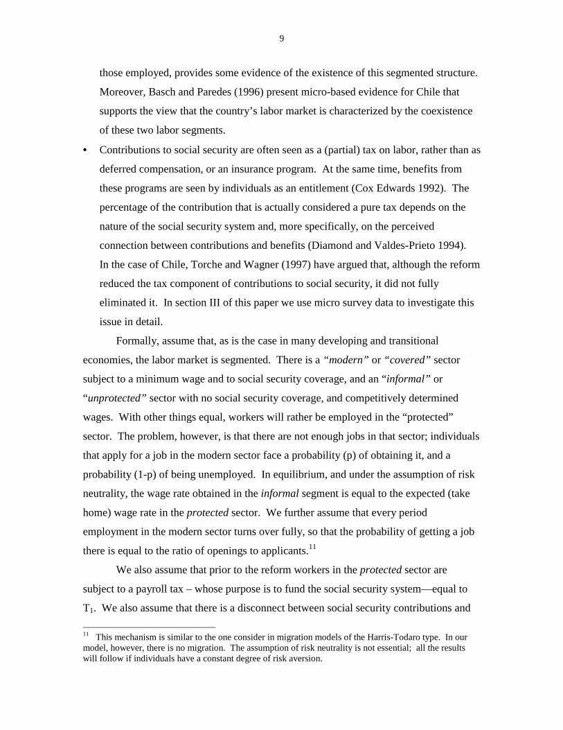
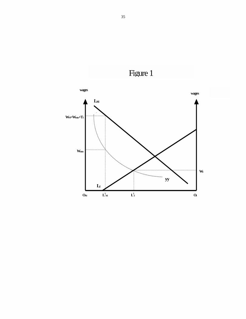
The initial (pre reform) labor market is depicted in Figure 1, under the simplifying

assumption that the unemployed get no assistance (S = 0). Distance O M - O I is total

labor supply, L M and L I are the demand for labor schedules, and yy is a rectangular

hyperbola, that satisfies the equilibrium condition in equation (1). The wage rate and the

level of employment in the informal sector are determined by the intersection of the yy

and L I schedules. W min is the minimum wage which, as stated above, is assumed to be

set in net take-home bases. T 1 is the payroll tax, and W M is the cost of labor in the

modern sector. W I is the wage rate in the informal sector. The initial level of

employment in the modern sector is given by distance O M – L M 1

; distance O I – L I 1

depicts initial employment in the informal sector. The total number of unemployed is

equal to distance L M 1

– L I 1 . In this model a social security reform that replaces a pay-

as-you-go regime with a capitalization one, has the effect of reducing the (perceived) tax

component of social security contributions. That is, there will be a reduction of T1, to

some lower level, possibly even to zero. This would unleash a series of effects, including

a higher demand for labor in the modern sector, a change in aggregate labor supply, and

changes in wages and in employment in the informal sector.

Formally, the model given by equations (1) - (11) can be solved to obtain the

effects of a social security reform, on a number of variables, including informal sector

wages (W I), the volume of unemployment (U), and product prices of in the informal

sector (P I). In order to simplify the exposition, we follow a long tradition in international

trade theory – the Ricardo-Viner approach – and we assume that capital is fixed in its

sector of origin. We begin with the effects of changes in the tax component of the social

security contribution (d log T)on informal sector wages (d log WI):

(12) d log W I = ∆ -1 { - [α U ( U / ( L M + U )) ( 1 / η M )]

- [( U / ( L M + U ) α M ( 1 / η M )]} ( T 1 / ( 1 + T1) ) d log T.

Where,

(13) ∆ = - α U - [α I ( U / ( L M + U )) ( 1 / η I ) ( µ - 1 )]

- [( U / ( L M + U )) φ (α I + µ β ) ].

13

α I , α M and α U are the shares of employment in the informal sector, employment in the

modern sector, and unemployment in the labor resources constraint (5). η I and η M are

the inverse of the elasticities of the demand for labor with respect to wages in the I and M

sectors, respectively, and are negative.14 φ is the supply elasticity of labor, and is

positive. µ is the elasticity of the price of informal sector goods (PI) with respect to the

wage rate in that sector, and is greater than zero and smaller than one. It follows from

equation (13), then, that ∆ is negative. Consequently, according to equation (12), the

following result holds:

(d log W I / d log T) < 0.

This means that a social security reform that reduces the pay roll tax, will unambiguously

generate an increase in the wage rate in I, the sector that is not covered by the by the

social security system. Notice that, by construction, net (take home) wages in the modern

sector are not affected by the reform. This is because we have assumed that the

minimum wage is set in take-home bases, and that the reform does not affect it. The

more general case where the reform generates an increase in net wages in the M sector is

discussed below.

The effect of the reform on aggregate unemployment (U), is given by:

(14) d log U = ∆ -1 { (α I / η I ) - [α I ( U / ( L M + U )) ( 1 / η I ) ( 1 / η M ) ( µ - 1 )]

- [( U / ( L M + U )) φ (α I + µ β ) ( 1 / η M )]} (T 1 / (1+T1)) d log T.

The sign of equation (14) is undetermined. It follows from this that within the

framework developed in this paper, a reduction in the payroll tax in the modern sector

will have an ambiguous effect on the number of unemployed. Whether the level of

unemployment will increase or decline will depend on two basic factors: the supply

elasticity of labor in the economy -- parameter φ in equation (14) --; and the demand

14 That is, η I = ( d log W I ) / ( d log L I ).

14

elasticity of labor demand in the informal sector. The more elastic is the supply for labor

and the more inelastic is the demand for labor in the informal sector, the more likely it is

that the reform will result in an increase in the level of unemployment.

Equation (15) gives the effect of the reform on product prices in the informal

sector, and is positive:

(15) d log P I = ∆ -1 { - ( U / ( L M + U )) (α M / η M )

- α U ( U / ( L M + U )) ( 1 / η M )} ( T 1 / ( 1 + T1 )) d log T.

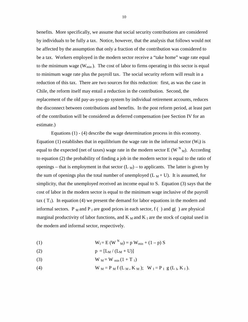
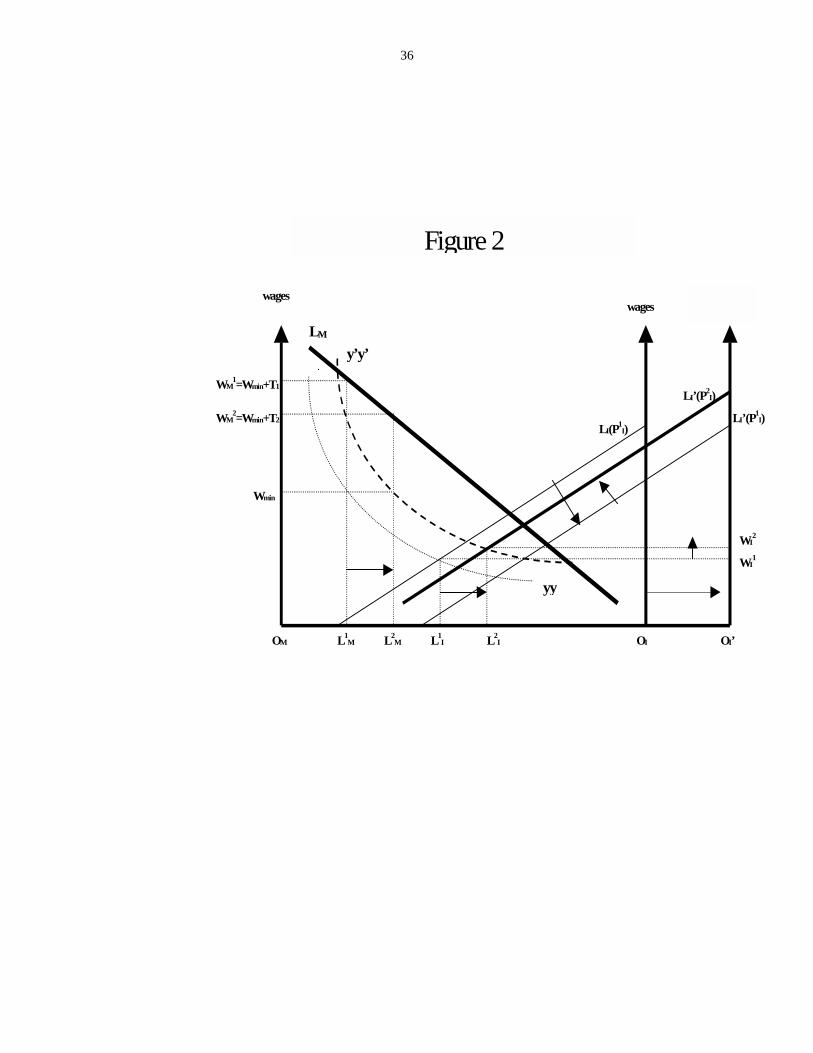
The working of the model is illustrated in Figure (2), where it is assumed that the

reform reduces the social security tax from T 1 to T 2. The new cost of labor in the

modern sector is WM2. Distance O I - O I’ is assumed to be equal to the increase in the

amount of labor supplied to the economy. Because of this increase in aggregate labor

supply, the original demand for labor in the informal sector has to be redrawn as LI’.

Since the product price of I has increased, the demand for labor in the informal sector

shifts up, and is represented in Figure 2 by L I’ (PI 1). The wage rate in the informal

sector is now determined by the intersection of a new rectangular hyperbola y’y’ and a

new demand for labor in sector I, and is given by W I2. Employment in the informal

sector has changed from distance O I – L I1 to distance O I1 – L I2. Because of the

reduction in W M, employment in the modern sector has increased from L M1 to L M2. The

new level of unemployment, which as indicated by equation (13), could be either higher

or lower than the initial level of unemployment, is given by distance L M2 - L I2 .

The results in equations (12) – (15) assume that there is no change in the take-

home wage in the modern sector. In Chile, however, the government mandated an

increase in take-home wages equal to 10 percent, for those that opted for the privatized

regime (Edwards 1998a). In the context of our model, an increase in the take-home wage

in the sector covered by social security can be modeled as an exogenously determined

increase in the minimum wage rate. Formally speaking, then, this more general policy

package corresponds to a situation where both the minimum wage (W min ) and the

payroll tax, change (in opposite directions). In this case the change in the wage rate in

the informal sector will be given by:

15

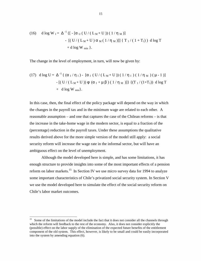
(16) d log W I = ∆ -1 {[ - [α U ( U / ( L M + U )) ( 1 / η M )]

- [( U / ( L M + U ) α M ( 1 / η M )]] { T 1 / ( 1 + T1) ) d log T

+ d log W min }.

The change in the level of employment, in turn, will now be given by:

(17) d log U = ∆ -1 { (α I / η I ) - [α I ( U / ( L M + U )) ( 1 / η I ) ( 1 / η M ) ( µ - 1 )]

- [( U / ( L M + U )) φ (α I + µ β ) ( 1 / η M )]} {(T 1 / (1+T1)) d log T

+ d log W min}.

In this case, then, the final effect of the policy package will depend on the way in which

the changes in the payroll tax and in the minimum wage are related to each other. A

reasonable assumption – and one that captures the case of the Chilean reforms – is that

the increase in the take-home wage in the modern sector, is equal to a fraction of the

(percentage) reduction in the payroll taxes. Under these assumptions the qualitative

results derived above for the more simple version of the model still apply: a social

security reform will increase the wage rate in the informal sector, but will have an

ambiguous effect on the level of unemployment.

Although the model developed here is simple, and has some limitations, it has

enough structure to provide insights into some of the most important effects of a pension

reform on labor markets.15 In Section IV we use micro survey data for 1994 to analyze

some important characteristics of Chile’s privatized social security system. In Section V

we use the model developed here to simulate the effect of the social security reform on

Chile’s labor market outcomes.

15 Some of the limitations of the model include the fact that it does not consider all the channels throughwhich the reform will feedback to the rest of the economy. Also, it does not consider explicitly the(possible) effect on the labor supply of the elimination of the expected future benefits of the entitlementcomponent of the old system. This effect, however, is likely to be small and could be easily incorporatedinto the system by amending equation (6).

16

IV. Chile’s New Pension System: Who Is Covered? How Much Do Participants

Value The System?

In this section we use micro survey data to analyze some key characteristics of

Chile’s privately managed social security system. Our basic data set is the CASEN

(Caracterización Socioeconómica Nacional) national survey for 1994. This is a

nationaly representative household survey put together by the National Planning Office.

The sample contains a total of 178,057 individual observations, including children and

the elderly. Of these, 111,643 correspond to individuals living in the urban areas, and

66,414 correspond to those in the rural areas. An urban area is defined as a grouping of

dwellings with a population in excess of 2,000 individuals. The survey collects

information on demographics, education, type of dwelling, health care, occupation,

employment, and income, among other variables. We are interested on two specific, and

interrelated, questions:

• What is the coverage of Chile’s privatized social security system? Or, in other

words, what percentage of those with a paying job, participate in the system?

This is a key issue within the context of the model developed in Section III of

this paper, where it was assumed that only a fraction of those in the labor

market – those employed in the “formal” sector – participate in the social

security system in an active way, making contributions to their own personal

retirement accounts.

• To what extent do participants in the system – and, more specifically, those

that are required by law to make contributions -- consider it a deferred

compensation scheme? A different way of putting the question is, to what

extent is the new system seen as having a tax component? This is an

important question within the model developed in this paper. In particular, it

plays a fundamental role in the simulation exercise on the effect of the reform

on labor market outcomes, and that we present in Section V.

Ideally we would like to use comparable data for the pre and post reform era.

This would allow us to understand the way in which the reform affected indivilual’s

17

behavior, and individuals perceptions. Unfortunately, however, detailed survey data have

only been collected since 1990.

IV.1 Extent of Coverage of Chile’s New Social Security System

According to the 1981 social security reform, those individuals that have an

employment contract are required to make contributions to their personal retirement

accounts.16 The self-employed and those in the informal sector may, if they so wish,

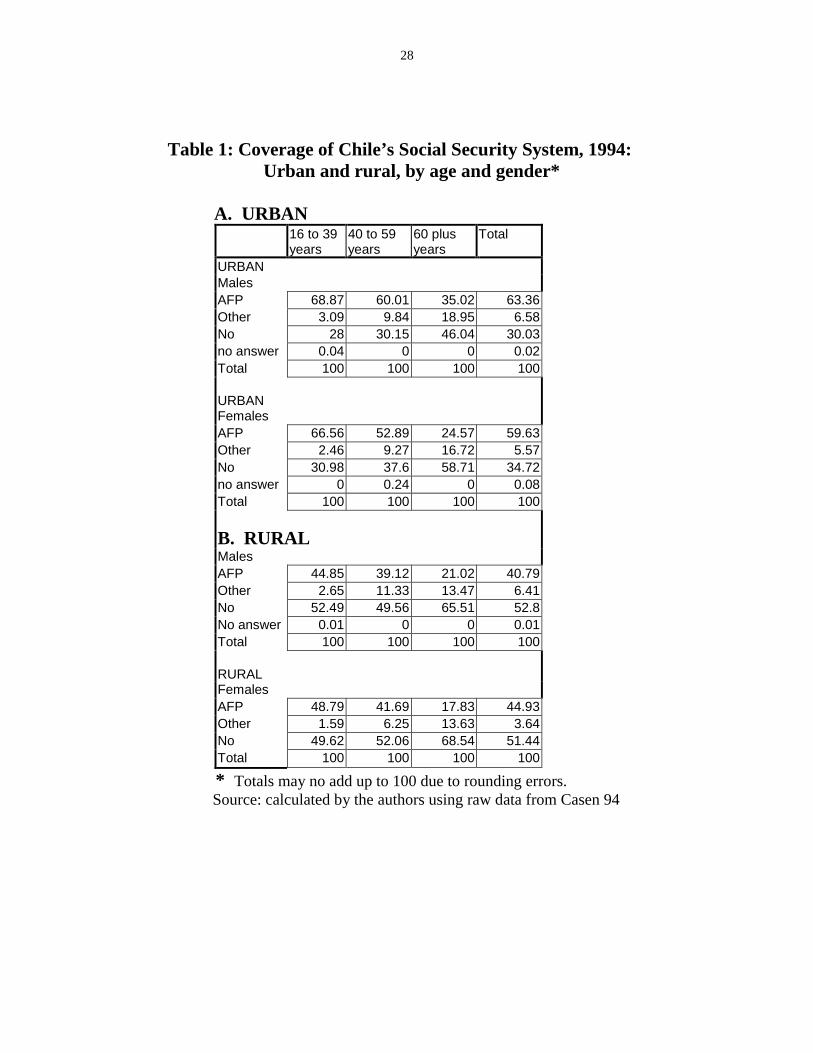
make voluntary contributions to the pension system. Table 1 presents summary data, for

1994, on coverage of the social security system. These data correspond to those

individuals in the sample that had a paying job at the time of the survey, and have been

organized by urban-rural sectors, age and gender. “AFP” refers to what percentage of

individuals in that particular group was making contributions to a privately managed

retirement fund (an AFP). “Other” refers to the percentage of individuals that were

making contributions to other retirement systems, including the old pay-as-you go system

and the armed forces retirement fund; “No” refers to those individuals that had not made

contributions to any retirement system.

The table is rather self-explanatory, and shows that as recently as 1994 Chile’s

system fell considerably short of universal coverage. Urban males have the highest rate

of total coverage – defined as contributing to any retirement scheme --, at 69.9 percent.

The lowest coverage corresponds to males in the rural sector, with 47.2%. It may also be

seen that, with the exception of rural males, those in the 16 to 39 year-old had the highest

degree of coverage. For the sample as a whole, in 1994 the coverage rate of the formal

retirement systems was 60.2%. Data from the CASEN survey suggests that there is a

very high degree of compliance with respect to required contributions. More that 95% of

employees with an employment contract made contributions, as required by law, to a

retirement system.

Although there are no comparable survey data for the pre reform period, existing

estimates indicates that Chile’s old pay-as-you-go system covered 58% of those

employed. This means, then, that after the privatization reform there has only been a

16 In many models of segmented labor markets, workers in the “formal” sector are defined as those withan employment contract. However, a broader definition – and one that we adopt in this paper – is thatworkers in the “formal” sector are those with employment contracts, plus those without contracts, but thatare covered by the formal pension system.

18

small increase in the coverage of the formal retirement system. The fact that younger

workers exhibit a higher coverage ratio may indicate, however, a secular trend towards

greater participation in the system.

IV.2 Deferred Compensation or Taxes?

The model developed in section III of this paper assumes that a reform of the

social security system implies a reduction in the (implicit) tax on labor. More

specifically, we assume that while under the pay-as-you-go system, contributions are

(largely) seen as taxes, under the privately managed regime they are seen as a deferred

compensation scheme. In this subsection we use data from the CASEN survey to

investigate the extent to which, on average, individuals indeed value the new privatized

system, and consider it as a component of their total compensation package.

For an individual employed in the formal sector, total labor compensation will be

equal to his take-home (cash) salary, plus a proportion of his mandated contribution to

the retirement system. If contributions are fully seen as deferred compensation, that

proportion will be equal to one. If on the other hand, contributions are fully seen as

taxes, that proportion will be equal to zero, and the total compensation will be only equal

to the take-home salary.17

In principle, the value attached by individuals to the pension system can be

estimated by comparing wages from jobs that are equivalent in all respects, except with

regard to contributions to the retirement program. If individuals value being enrolled in

the pension’s program, we would expect that, for otherwise equivalent jobs, the take-

home pay of those that participate in the system will be lower than that of individuals that

do not make contributions. The actual difference in the (cash) take-home pay can, then,

be attributed to the value that individuals attach to being members of the retirement

system.

Chile’s specific institutional arrangements, however, complicate our task of

estimating the imputed value of mandated social security contributions from a wage

equation. The main difficulty stems from the fact that the law requires individuals to

make contributions not only to the retirement system (at 10% of wages), but also to the

17 This, however, is only a first order approximation. The actual proportion of the contribution willdepend on the individual’s rate of discount, and the pension fund’s rate of return, among other things.

19

health system (7%) and to a mandated life insurance program (3%). Total contributions

for this “package,” stand at 20% of wages (up to a maximum), significantly lower than

the 43% required under the traditional system. A second complication is that individuals

have a choice with respect to the health care component of the package. They can either

opt for a basic, public sector-run program known as FONASA, or they can use the 7%

health contribution towards the purchase of a privately provided health insurance policy.

This latter option is known as ISAPRE, and its cost tends to exceed the 7% mandated

health contribution. This means that, in practice, those that participate in the system have

to choose between a “retirement-cum-basic health” package, or a “retirement-cum-

private health insurance” package. Our estimation of a wage equation, explicitly takes

this option into account.18

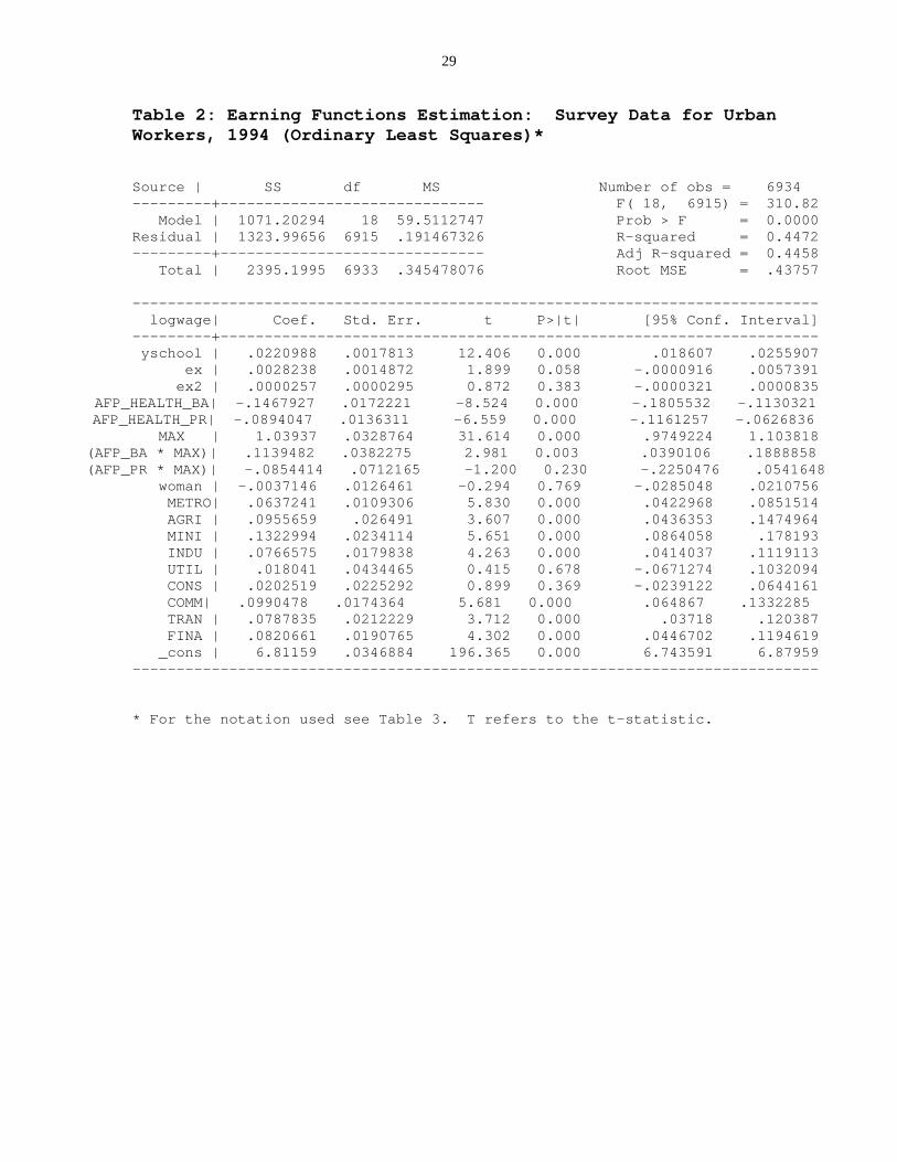
In Table 2 we present the results obtained from the estimation of a wage equation

for 1994. The sample has 6,934 observations, and is comprised of civilian workers in the

urban sector, that held a paying job, did not receive retirement benefits at the time of the

survey, and whose salary was in the top quintile of the wage distribution. The dependent

variable is the log of hourly net (take-home) wages; the notation used for the independent

variables is provided in Table 3. We control for the usual variables that explain wage

differentials, including schooling, experience, geographical location, gender and industry.

We also control for earnings in excess of the maximum amount subject to social security

contributions: “MAX” is a dummy that takes a value of one if the individual’s salary

exceeds that maximum. Our main interest is to obtain an estimate of the effect of

contributions on wage differentials. We do this by introducing two dummy variables into

the analysis: “AFP_HEALTH_BA” is a dummy that takes a value of one if the

individual in question has made contributions to the “retirement-cum-basic health”

package. “AFP_HEALTH_PR” is a dummy that takes a value of one if the individual in

question has opted for the “retirement-cum-private health insurance” package. These

variables were introduced both on their own, as well as interacted with the MAX dummy.

As may be seen from Table 2, the estimated coefficients for the traditional

variables – schooling, experience and experienced squared – are along the line of what is

18 This choice is affected by income. By focusing our estimation effort on the top quintile of thedistribution we hope to capture the relationship between contributions and wages, rather than betweenincome and the choice of health program.

20

expected, and are consistent with previous estimates for Chile and other emerging

economies. The coefficient for the geographical dummy capturing the metropolitan area

is significant, as are most of the coefficients for industry. More important for our

analysis, however, is that the estimated coefficient for both the AFP_HEALTH_BA and

AFP_HEALTH_PR dummies are negative and highly significant. Their point estimates,

-0.147 and –0.089 respectively, however, are smaller (in absolute value) than the

mandated contribution of 20%. This suggests that, after controlling for other factors such

as schooling, experience, industry, and geographical region, individuals that make

required contributions to the retirement-health-insurance system, have lower hourly net

earnings that are those individuals that are not in the system.19

To the extent that an individual freely chooses to be employed in a job that

requires him to make contributions, rather than in one that does not require them, the

coefficients of AFP_HEALTH_BA and AFP_HEALTH_PR can be interpreted as

capturing the value attached to these packages. The fact that the estimates of both

contribution dummies are lower (in absolute terms) than the 20% mandatory contribution

rate, suggests that, although individuals attached a positive value to the social security

package, they attached a value that was somewhat lower than the actual contribution..

The results in Table 2 also indicate that the coefficient of AFP_HEALTH_BA

interacted with MAX is insignificantly different from zero. We interpret this is indicating

that individuals with income above MAX, that are enrolled in the “retirement-cum-basic

health” package, attach to it the same value participants with income below MAX.

Interestingly enough, the coefficient of AFP_HEALTH_PR interacted with MAX is

significantly positive, with a point estimate of 0.114. Moreover, it is not possible to

reject the hypothesis that the sum of AFP_HEALTH_PR and (AFP_HEALTH_PR *

MAX) is different from zero. The F-statistic for this restriction is 0.46 and has a p-value

of 0.49. This result can be interpreted as indicating that those in the upper tail of the

income distribution place no value to mandatory contributions.20 A limitation of the

estimates in table 2, is that it is not possible to precisely disentangle by how much

19 This is strictly the case if the individual wage is below the maximum wage subject to contributions. Seethe discussion below.20 This, however, is not relevant for our simulation exercise. What matters is the marginal value attachedto the system. This is captured by the contribution dummy variables.

21

participants value each of the components of the mandatory package. In the simulation

exercises presented in section V we assume that the proportional value is the same across

the three components of the package.

In order to investigate for the robustness of the results reported in Table 2, we

estimated additional earnings equations for alternative samples. We also used a two

stages procedure to deal with possible endogeneity problems. The results obtained from

these alternative estimations, confirmed those reported in Table 2, and are not presented

here due to space considerations. In section V of this paper we use the estimates reported

in Table 2 as am input into our simulation exercises.

V. Chile’s Pension Reform And The Labor Market

In this section we present the results from simulation exercises, based on the

model derived in section III, on the effects of the social security reform on Chile’s labor

market. Values for the key parameters were taken from other studies of the Chilean

economy, as well as from the econometric results presented in the previous section.

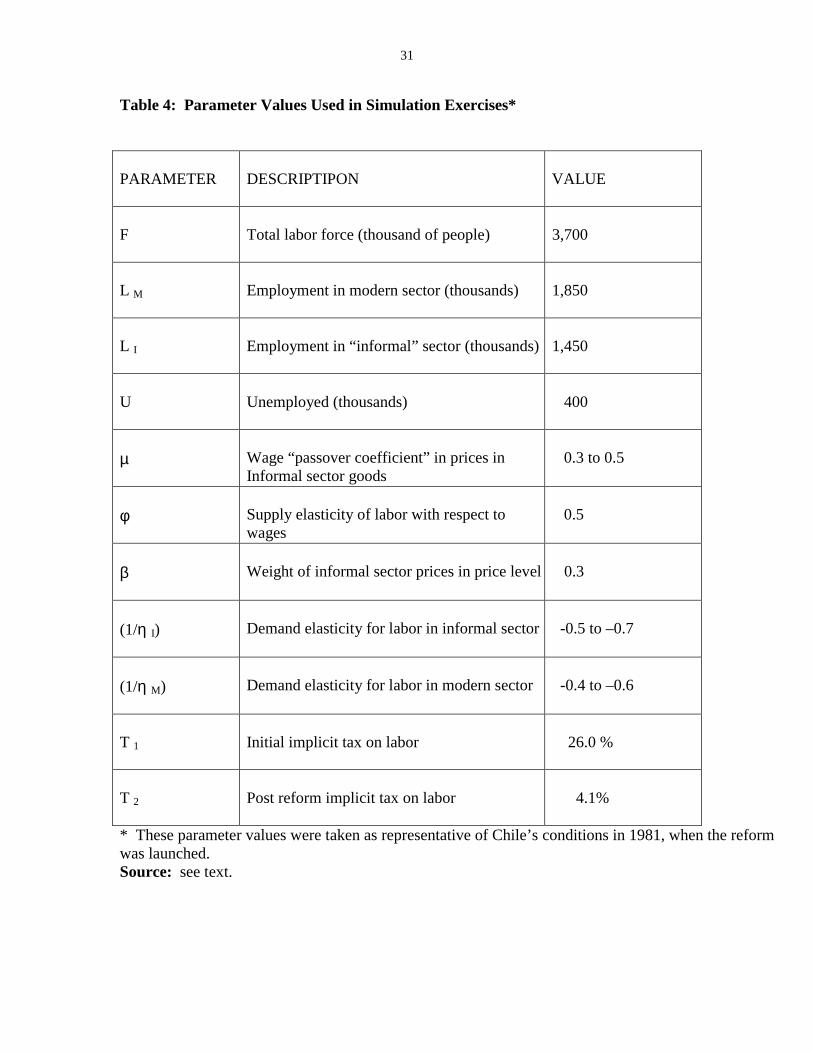
In Table 4 we present the values of the parameters used in the simulation exercise.

The elasticities were taken from Coeymans and Mundlack (1993). The data on the labor

force and the rate of unemployment were taken from Banco Central de Chile. The

percentage of workers in the informal sector was taken from the analysis reported in

section IV of this paper. The parameter for µ was taken from a number of studies on

Chile’s inflation. We assumed that under the traditional pay-as-you-go system,

contributions to the social security system (at an average rate of 26% of wages) were

fully considered to be a tax; as pointed out above, benefits during the pre-reform era were

considered to be an entitlement. Finally, we assumed that in the post reform period,

mandated contributions to the pension system had a tax component equal to 4.1% of

wages. That is, we assume that individuals considered that approximately 40 percent of

the required contribution to the pension fund constituted a tax. This figure is based on

the econometric results reported in the preceding section. More specifically, it was

obtained after averaging the imputed “tax” component obtained from the two

“contribution” dummies in the regression reported in Table 2, and assuming that the

22

estimated “tax” component of contributions to the pension-health-insurance package, is

equal across the three components of the package.21

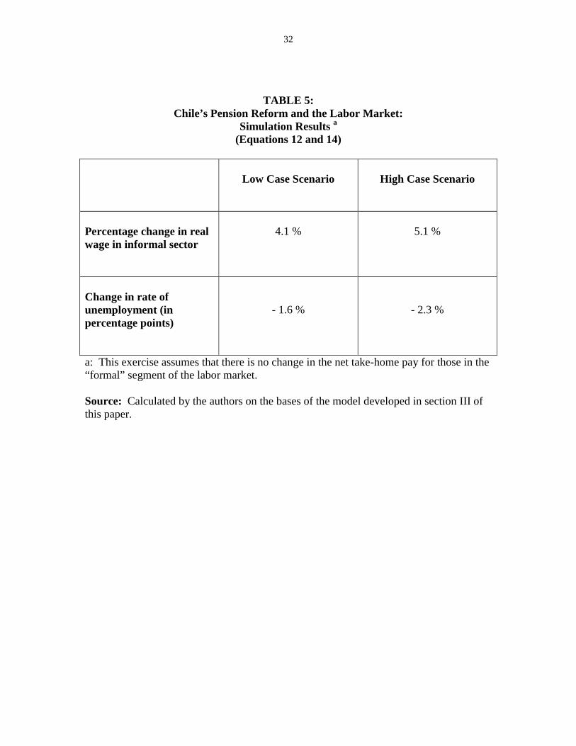
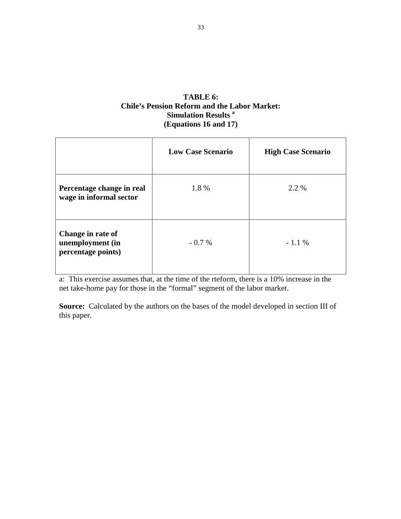
In Table 5 we present the simulation results for the case where the reform reduces

the (implicit) tax on labor, but where there is no increase in the take-home pay for those

enrolled in the system. These results were obtained after calibrating equations (12) and

(14) in Section III. Table 6, on the other hand, contains the results from the simulation

exercise, when it is assumed that the reform results in a 10% increase in net take-home

pay for those enrolled in the system, and correspond to equations (16) and (17). In both

tables we have presented a “low” and a “high” case scenario. As may be seen, these

results suggest that, by reducing the implicit tax on labor, Chile’s pension reform had a

positive effect on wages in the informal sector, at the same time as it contributed to a

reduction in the rate of unemployment.

The results in Table 6, which are based on assumptions that closely capture

Chile’s experience, suggest that the actual effect of the pension reform on labor market

outcomes was rather modest with respect to unemployment reduction. According to our

simulation exercise, in the high case scenario, the reforms only contributed 1.1

percentage points to the reduction of the rate of unemployment. The total effect on net

wages was significant, however: first, net wages in the formal sector increased by 10%;

second, wages in the informal sector increased between 1.8 and 2.2 percent. This

translates into a weighted average increase for net wages in the range of 6.3 to 6.6%.

From a distributional point of view, these results indicate that the benefits of the reforms

were greater to those in the formal and covered sector, where wages and job conditions

usually tend to be better than in the informal sector.

VI. Concluding Remarks

In 1981, Chile reformed its social security system. An inefficient and insolvent

pay-as-you-go regime was replaced by system based on individual retirement accounts.

Over the years Chile’s reform has been widely praised, and has been carefully studied by 21 The results in Table 2 suggest that, after controlling for other factors, those individuals that are subjectto mandated contributions (at a 20% rate), have a take-home pay that is on average 11.8% below that ofindividuals that don’t participate in the system (This is the average of the two dummies point estimates:

23

policy makers throughout the world. In this paper we have focused on a neglected aspect

of Chile’s social security reform: its impact on labor market outcomes, including

unemployment and wages. We develop a model of the labor market where we assume

that, as is the case in most emerging markets, a formal and an informal sectors coexist

side by side.

According to our model, a social security reform that reduces the implicit tax on

labor in the formal sector – as was the case in Chile --, will result in an increase in the

wage rate in the informal sector. The effect of this type of reform on aggregate

unemployment is undetermined, however. Results from simulation exercises suggest that

in the case of Chile the reforms resulted in an increase in informal sector wages between

2 an 2.5%. These results also suggest that the reforms made a positive contribution to the

reduction of Chile’s aggregate of unemployment.

0.118 = (0.147+0.089)/2. The estimated perceived tax of the pension component is, then, calculated as (1-0.118 / 0.2) x 0.1 = 0.041.

24

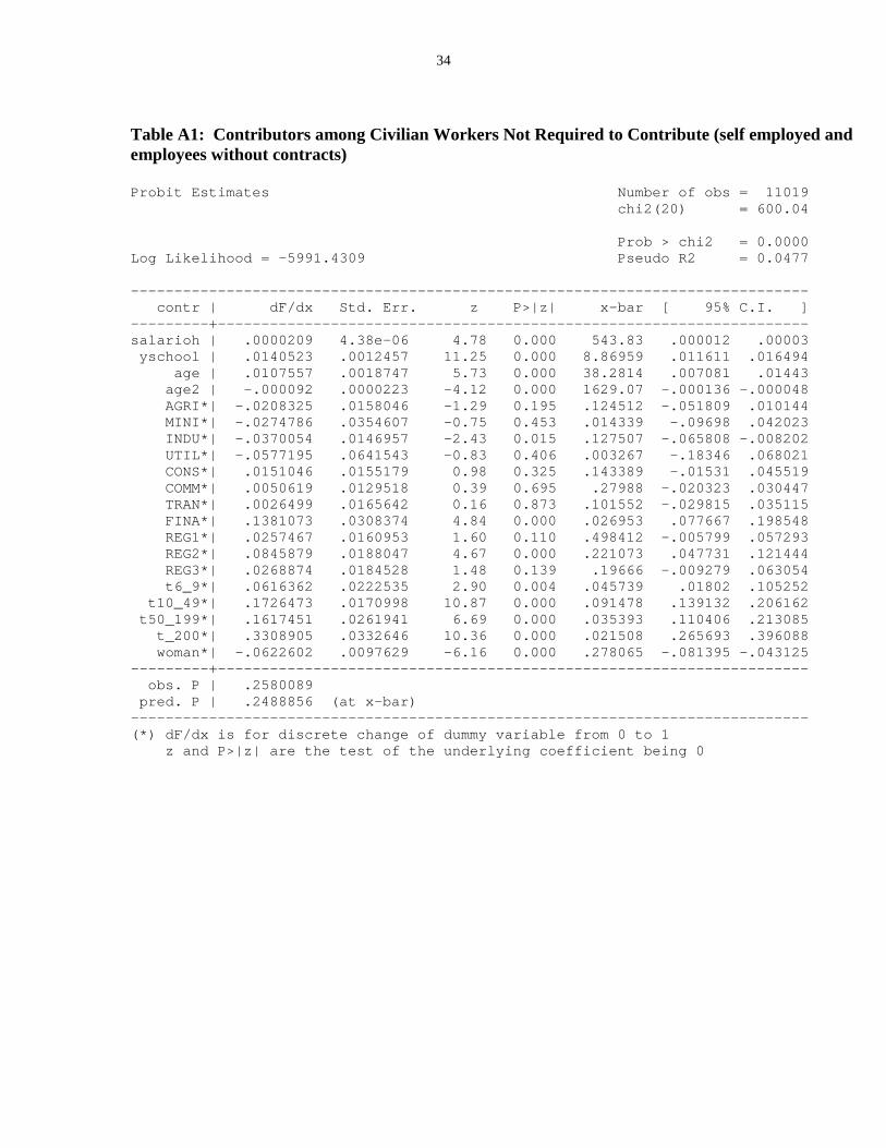
APPENDIX

To Contribute or not to Contribute? That is the Question

According to the 1994 CASEN survey, 25.8% of individuals that were not

required by law to be enrolled in the system, still made voluntary contributions to an

individual retirement account.

What are the characteristics of those individuals that voluntarily participated in

the retirement system? In order to address this issue, we estimated a number of probit

equation for the probability of making (voluntary) contributions. In estimating this

regression we defined a dummy variable that took the value of one if the individual in

question had made contributions to a retirement account, and zero if he did not make

contributions. The results obtained from the basic regression are reported in Table A1. In

this estimate, the sample had 11,019 observations, corresponding to urban sector

individuals with a paying job, and that did not have an employment contract. As is

customary, we report the change in the probability of being enrolled as a result of a

change in the independent variable (column dF/dx). A detailed description of the

notation for the independent variables used in the probit regression analysis is provided in

Table 3 in the text of the paper.

Several interesting results emerge from the probit regressions reported in Table

A1. First, after controlling for other factors, a higher hourly salary increases slightly (but

significantly) the probability of making voluntary contributions to a retirement account.

Second, a higher number of years of schooling, also increases the probability of

contributing to a retirement account. Third, age increases the probability of contributing,

but at a decreasing rate (the coefficient of age squared is significantly negative). Fourth,

only two of the sectoral dummies are significant. Those in financial services have a

higher probability of contributing, while those in the industrial sector have a lower

probability of doing so. Fifth, only one regional dummy – the one corresponding to the

center of the country -- is significant. Sixth, working in a firm with more than six co-

workers increases the probability of making voluntary contributions. Finally, after

controlling for other factors, women have a significantly lower probability of

participating in a privately managed retirement system.

25

In order to check for the robustness of these results, we estimated similar Probit

regressions for different samples, including one with over 35,000 observations,

corresponding to urban workers with and without an employment contracts. Generally

speaking, the results obtained from those estimates, coincide with those obtained with the

smaller sample and reported in Table A1. The only important difference refers to the

sectoral dummies. According to these estimates – available on request – those in the

construction, commerce and agriculture sector have a lower probability of making

contributions to the retirement system.

26

References

Arellano, Josg Pablo. 1982a. ^Elementos para el anYlisis de la reforma de la previsiynsocial chilena.] El Trimestre Econymico 49 (3) (July-Sept.): 563-605.

Arellano, Josg Pablo. 1982b. ^Efectos macroeconymicos de la reforma previsionalchilena.] Cuadernos de Economoa 56 (abril): 111-22.

Arrau, Patricio. 1991. ^La reforma previsional chilena y su financiamiento durante latransiciyn.] Colecciyn Estudios CIEPLAN 32 (June): 5-44.

Bach,M. and Ricardo Paredes (1996) “Are There Dual Labor Markets in Chile?:Empirical Evidence”, Journal-of-Development-Economics; 50(2), August 1996, pages297-312..

Baeza Valdgs, Sergio, and Ra‚l Burger Torres. 1995. ^Calidad de las pensiones delsistema privado chileno.] In Quince awos despues: Una mirada al sistema privado depensiones, edited by S. Baeza and F. Margozzini. Santiago: Centro de Estudios P‚blicos.

Bosworth, Barry P.; Dornbusch, Rudiger, and Ra‚l LabYn, editors. 1994. The ChileanEconomy: Policy Lessons and Challenges. Washington, DC: The Brookings Institution.

Bustamante Jeraldo, Julio. 1995. ^Principales cambios legales al DL 3.500 en el peroodonoviembre 1990-Mayo 1995 y Desafoos Pendientes.] In Quince awos despues: Unamirada al sistema privado de pensiones, edited by S. Baeza and F. Margozzini. Santiago:Centro de Estudios P‚blicos.

Cifuentes, Rodrigo S. 1995. ^Reforma de los sistemas previsionales: Aspectosmacroeconymicos.] Cuadernos de Economoa 96 (agosto): 217-50.

Coeymans and Mundlack, 1993. “Sectoral growth in Chile: 1962-82”, Research Report,vol. 95. Washington, D.C.: International Food Policy Research Institute,

Cox-Edwards, Alejandra. 1992. ^Economic Reform and Labor Market Legislation inLatin America.] California State University, mimeo.

Davis, E. P.1998. “”Pensions in the Corporate Sector”, in Redesigning Social Security,H. Siebert (Ed.)

Diamond, Peter. 1994. ^Privatization of Social Security: Lessons from Chile.] Revista deAnYlisis Econymico 9 (1) (June): 21-34.

Diamond, Peter and Salvador Valdgs-Prieto. 1994. ^Social Security Reforms.] In TheChilean Economy: Policy Lessons and Challenges, edited by B. Bosworth, R. Dornbuschand R. LabYn. Washington, DC: The Brookings Institution

27

Edwards, Sebastian. 1995. Crisis and Reform in Latin America: From Despair to Hope.New York: Oxford University Press.

Edwards, Sebastian, 1998a. “ The Chilean Pension Reform: A Pioneering Program”, inPrivatizing Social Security, by M. Feldsrein (ed.).

Edwards, Sebastian, 1998b. “ Chile: Radical Change Towards a Funded System” inRedesigning Social Security, H. Siebert (Ed.)

Edwards, Sebastian, and Alejandra Edwards. 1991. Monetarism and Liberalization: TheChilean Experiment. Chicago: University of Chicago Press, second edition.

Edwards, Sebastian, and Alejandra Edwards. 1999.Economic Reforms and Labor Market:Policy Eissues and Lessons from Chile. Paper presented at the Economic PolicyMeeting, Frankfurt, April 1999

Fontaine, Juan Andrgs. 1994. ^Inversiones extranjeras por fondos de pensiones: Efectossobre la polotica macroeconymica.] Cuadernos de Economoa 93 (agosto): 161-183.

Fuentes Silva, Roberto. 1995. ^Evoluciyn y resultados del sistema.] In Quince awosdespues: Una mirada al sistema privado de pensiones, edited by S. Baeza and F.Margozzini. Santiago: Centro de Estudios P‚blicos.

Gruber J. and D. A. Wise, (Eds) 1999. Social Security and Retirement around the World,University of Chicago Press.

Iglesias, A. and D. Vittas, 1992. ^The Rationale and Performance of Personal PensionPlans in Chile], Working Paper 867, The World Bank.

Lorz, Oliver. 1998. "Social Security and Employment", in Redesigning Social Security,H. Siebert (Ed.)

Schmidt-Hebbel, K. 1997. “Pension Reform, Informal markets and Long term Incomeand Welfare.” Working paper, Banco Central de chile.

Siebert, Horst. 1998. "Pay-as-you-go versus capital funded Pension systems. The Issues"in Redesigning Social Security, H. Siebert (Ed.)

Torche, A. And Gert Wagner, 1997. “Prevision Social: Valoracion Individual de unBeneficio Mandatado”. Cuandernos de Economia, N 103, pp. 363-390.

World Bank, 1994. The Old Age Crisis, Washington, D.C.

28

Table 1: Coverage of Chile’s Social Security System, 1994:Urban and rural, by age and gender*

A. URBAN16 to 39years

40 to 59years

60 plusyears

Total

URBANMalesAFP 68.87 60.01 35.02 63.36Other 3.09 9.84 18.95 6.58No 28 30.15 46.04 30.03no answer 0.04 0 0 0.02Total 100 100 100 100

URBANFemalesAFP 66.56 52.89 24.57 59.63Other 2.46 9.27 16.72 5.57No 30.98 37.6 58.71 34.72no answer 0 0.24 0 0.08Total 100 100 100 100

B. RURALMalesAFP 44.85 39.12 21.02 40.79Other 2.65 11.33 13.47 6.41No 52.49 49.56 65.51 52.8No answer 0.01 0 0 0.01Total 100 100 100 100

RURALFemalesAFP 48.79 41.69 17.83 44.93Other 1.59 6.25 13.63 3.64No 49.62 52.06 68.54 51.44Total 100 100 100 100

* Totals may no add up to 100 due to rounding errors. Source: calculated by the authors using raw data from Casen 94

29

Table 2: Earning Functions Estimation: Survey Data for UrbanWorkers, 1994 (Ordinary Least Squares)*

Source | SS df MS Number of obs = 6934---------+------------------------------ F( 18, 6915) = 310.82

Model | 1071.20294 18 59.5112747 Prob > F = 0.0000Residual | 1323.99656 6915 .191467326 R-squared = 0.4472---------+------------------------------ Adj R-squared = 0.4458

Total | 2395.1995 6933 .345478076 Root MSE = .43757

------------------------------------------------------------------------------logwage| Coef. Std. Err. t P>|t| [95% Conf. Interval]

---------+--------------------------------------------------------------------yschool | .0220988 .0017813 12.406 0.000 .018607 .0255907

ex | .0028238 .0014872 1.899 0.058 -.0000916 .0057391ex2 | .0000257 .0000295 0.872 0.383 -.0000321 .0000835

AFP_HEALTH_BA| -.1467927 .0172221 -8.524 0.000 -.1805532 -.1130321AFP_HEALTH_PR| -.0894047 .0136311 -6.559 0.000 -.1161257 -.0626836

MAX | 1.03937 .0328764 31.614 0.000 .9749224 1.103818(AFP_BA * MAX)| .1139482 .0382275 2.981 0.003 .0390106 .1888858(AFP_PR * MAX)| -.0854414 .0712165 -1.200 0.230 -.2250476 .0541648

woman | -.0037146 .0126461 -0.294 0.769 -.0285048 .0210756METRO| .0637241 .0109306 5.830 0.000 .0422968 .0851514AGRI | .0955659 .026491 3.607 0.000 .0436353 .1474964MINI | .1322994 .0234114 5.651 0.000 .0864058 .178193INDU | .0766575 .0179838 4.263 0.000 .0414037 .1119113UTIL | .018041 .0434465 0.415 0.678 -.0671274 .1032094CONS | .0202519 .0225292 0.899 0.369 -.0239122 .0644161COMM| .0990478 .0174364 5.681 0.000 .064867 .1332285TRAN | .0787835 .0212229 3.712 0.000 .03718 .120387FINA | .0820661 .0190765 4.302 0.000 .0446702 .1194619

_cons | 6.81159 .0346884 196.365 0.000 6.743591 6.87959------------------------------------------------------------------------------

* For the notation used see Table 3. T refers to the t-statistic.

30

Table 3: Notation Used in Empirical Analysis

logwage: log of hourly wages

yschool Years of schooling

ex Experience

exp Experience squared

AGRI Dummy for agriculture

MINI Mining

INDU Industry

UTIL Utilities

CONS Construction

COMM Commerce

TRAN Transportation

FINA Financial services

METRO Workers in the two largest metropolitan areas

MAX Dummy that takes value of one if wage exceeds maximum

subject to social security contributions

AFP_HEALTH_BA Dummy that takes value of one if individual is enrolled in the

social security program and in the basic health service

program

AFP_HEALTH_PR Dummy that takes value of one if individual is enrolled in the

social security program and in a private health insurance

program

(AFP _BA * MAX) Variable that interacts AFP_HEALTH_BA and MAX

(AFP_PR * MAX) Variable that interacts AFP_HEALTH_PR and MAX

Woman Dummy that takes a value of one if the individual is a woman

31

Table 4: Parameter Values Used in Simulation Exercises*

PARAMETER DESCRIPTIPON VALUE

F Total labor force (thousand of people) 3,700

L M Employment in modern sector (thousands) 1,850

L I Employment in “informal” sector (thousands) 1,450

U Unemployed (thousands) 400

µ Wage “passover coefficient” in prices inInformal sector goods

0.3 to 0.5

φ Supply elasticity of labor with respect towages

0.5

β Weight of informal sector prices in price level 0.3

(1/η I) Demand elasticity for labor in informal sector -0.5 to –0.7

(1/η M) Demand elasticity for labor in modern sector -0.4 to –0.6

T 1 Initial implicit tax on labor 26.0 %

T 2 Post reform implicit tax on labor 4.1%

* These parameter values were taken as representative of Chile’s conditions in 1981, when the reformwas launched.Source: see text.

32

TABLE 5:Chile’s Pension Reform and the Labor Market:

Simulation Results a(Equations 12 and 14)

Low Case Scenario High Case Scenario

Percentage change in realwage in informal sector

4.1 % 5.1 %

Change in rate ofunemployment (inpercentage points)

- 1.6 % - 2.3 %

a: This exercise assumes that there is no change in the net take-home pay for those in the“formal” segment of the labor market.

Source: Calculated by the authors on the bases of the model developed in section III ofthis paper.

33

TABLE 6:Chile’s Pension Reform and the Labor Market:

Simulation Results a(Equations 16 and 17)

Low Case Scenario High Case Scenario

Percentage change in realwage in informal sector

1.8 % 2.2 %

Change in rate ofunemployment (inpercentage points)

- 0.7 % - 1.1 %

a: This exercise assumes that, at the time of the rteform, there is a 10% increase in thenet take-home pay for those in the “formal” segment of the labor market.

Source: Calculated by the authors on the bases of the model developed in section III ofthis paper.

34

Table A1: Contributors among Civilian Workers Not Required to Contribute (self employed andemployees without contracts)

Probit Estimates Number of obs = 11019chi2(20) = 600.04

Prob > chi2 = 0.0000Log Likelihood = -5991.4309 Pseudo R2 = 0.0477

------------------------------------------------------------------------------contr | dF/dx Std. Err. z P>|z| x-bar [ 95% C.I. ]

---------+--------------------------------------------------------------------salarioh | .0000209 4.38e-06 4.78 0.000 543.83 .000012 .00003yschool | .0140523 .0012457 11.25 0.000 8.86959 .011611 .016494

age | .0107557 .0018747 5.73 0.000 38.2814 .007081 .01443age2 | -.000092 .0000223 -4.12 0.000 1629.07 -.000136 -.000048AGRI*| -.0208325 .0158046 -1.29 0.195 .124512 -.051809 .010144MINI*| -.0274786 .0354607 -0.75 0.453 .014339 -.09698 .042023INDU*| -.0370054 .0146957 -2.43 0.015 .127507 -.065808 -.008202UTIL*| -.0577195 .0641543 -0.83 0.406 .003267 -.18346 .068021CONS*| .0151046 .0155179 0.98 0.325 .143389 -.01531 .045519COMM*| .0050619 .0129518 0.39 0.695 .27988 -.020323 .030447TRAN*| .0026499 .0165642 0.16 0.873 .101552 -.029815 .035115FINA*| .1381073 .0308374 4.84 0.000 .026953 .077667 .198548REG1*| .0257467 .0160953 1.60 0.110 .498412 -.005799 .057293REG2*| .0845879 .0188047 4.67 0.000 .221073 .047731 .121444REG3*| .0268874 .0184528 1.48 0.139 .19666 -.009279 .063054t6_9*| .0616362 .0222535 2.90 0.004 .045739 .01802 .105252

t10_49*| .1726473 .0170998 10.87 0.000 .091478 .139132 .206162t50_199*| .1617451 .0261941 6.69 0.000 .035393 .110406 .213085

t_200*| .3308905 .0332646 10.36 0.000 .021508 .265693 .396088woman*| -.0622602 .0097629 -6.16 0.000 .278065 -.081395 -.043125

---------+--------------------------------------------------------------------obs. P | .2580089

pred. P | .2488856 (at x-bar)------------------------------------------------------------------------------(*) dF/dx is for discrete change of dummy variable from 0 to 1

z and P>|z| are the test of the underlying coefficient being 0

35

Figure 1

OM L1M L1

I OI

LM

yyLI

WM=Wmin+T1

Wmin

WI

wageswages

36

Figure 2

OM L1M L1

I OI

LM

yy

LI(P1I)

WM1=Wmin+T1

Wmin

WI1

wageswages

LI’(P2I)

LI’(P1I)

L2I OI’L2

M

WM2=Wmin+T2

WI2

y’y’