Embed Size (px)
Citation preview
Solutions to Exercises Marked with s©from the book
Introduction to Probability by
Joseph K. Blitzstein and Jessica Hwangc© Chapman & Hall/CRC Press, 2014
Joseph K. Blitzstein and Jessica HwangDepartments of Statistics, Harvard University and Stanford University


Chapter 1: Probability and counting
Counting
8. s© (a) How many ways are there to split a dozen people into 3 teams, where one teamhas 2 people, and the other two teams have 5 people each?
(b) How many ways are there to split a dozen people into 3 teams, where each team has4 people?
Solution:
(a) Pick any 2 of the 12 people to make the 2 person team, and then any 5 of theremaining 10 for the first team of 5, and then the remaining 5 are on the other team of5; this overcounts by a factor of 2 though, since there is no designated “first” team of5. So the number of possibilities is
(122
)(105
)/2 = 8316. Alternatively, politely ask the 12
people to line up, and then let the first 2 be the team of 2, the next 5 be a team of 5,and then last 5 be a team of 5. There are 12! ways for them to line up, but it does notmatter which order they line up in within each group, nor does the order of the 2 teamsof 5 matter, so the number of possibilities is 12!
2!5!5!·2 = 8316.
(b) By either of the approaches above, there are 12!4!4!4!
ways to divide the people into aTeam A, a Team B, and a Team C, if we care about which team is which (this is calleda multinomial coefficient). Since here it doesn’t matter which team is which, this overcounts by a factor of 3!, so the number of possibilities is 12!
4!4!4!3!= 5775.
9. s© (a) How many paths are there from the point (0, 0) to the point (110, 111) in theplane such that each step either consists of going one unit up or one unit to the right?
(b) How many paths are there from (0, 0) to (210, 211), where each step consists of goingone unit up or one unit to the right, and the path has to go through (110, 111)?
Solution:
(a) Encode a path as a sequence of U ’s and R’s, like URURURUUUR . . . UR, whereU and R stand for “up” and “right” respectively. The sequence must consist of 110 R’sand 111 U ’s, and to determine the sequence we just need to specify where the R’s arelocated. So there are
(221110
)possible paths.
(b) There are(221110
)paths to (110, 111), as above. From there, we need 100 R’s and 100
U ’s to get to (210, 211), so by the multiplication rule the number of possible paths is(221110
)·(200100
).
Story proofs
15. s© Give a story proof that∑nk=0
(nk
)= 2n.
Solution: Consider picking a subset of n people. There are(nk
)choices with size k, on
the one hand, and on the other hand there are 2n subsets by the multiplication rule.
1
2 Chapter 1: Probability and counting
16. s© Show that for all positive integers n and k with n ≥ k,(n
k
)+
(n
k − 1
)=
(n+ 1
k
),
doing this in two ways: (a) algebraically and (b) with a story, giving an interpretationfor why both sides count the same thing.
Hint for the story proof: Imagine n + 1 people, with one of them pre-designated as“president”.
Solution:
(a) For the algebraic proof, start with the definition of the binomial coefficients in theleft-hand side, and do some algebraic manipulation as follows:(
n
k
)+
(n
k − 1
)=
n!
k!(n− k)!+
n!
(k − 1)!(n− k + 1)!
=(n− k + 1)n! + (k)n!
k!(n− k + 1)!
=n!(n+ 1)
k!(n− k + 1)!
=
(n+ 1
k
).
(b) For the story proof, consider n + 1 people, with one of them pre-designated as“president”. The right-hand side is the number of ways to choose k out of these n + 1people, with order not mattering. The left-hand side counts the same thing in a differentway, by considering two cases: the president is or isn’t in the chosen group.
The number of groups of size k which include the president is(nk−1
), since once we fix
the president as a member of the group, we only need to choose another k− 1 membersout of the remaining n people. Similarly, there are
(nk
)groups of size k that don’t include
the president. Thus, the two sides of the equation are equal.
18. s© (a) Show using a story proof that(k
k
)+
(k + 1
k
)+
(k + 2
k
)+ · · ·+
(n
k
)=
(n+ 1
k + 1
),
where n and k are positive integers with n ≥ k. This is called the hockey stick identity.
Hint: Imagine arranging a group of people by age, and then think about the oldestperson in a chosen subgroup.
(b) Suppose that a large pack of Haribo gummi bears can have anywhere between 30and 50 gummi bears. There are 5 delicious flavors: pineapple (clear), raspberry (red),orange (orange), strawberry (green, mysteriously), and lemon (yellow). There are 0 non-delicious flavors. How many possibilities are there for the composition of such a pack ofgummi bears? You can leave your answer in terms of a couple binomial coefficients, butnot a sum of lots of binomial coefficients.
Solution:
(a) Consider choosing k+1 people out of a group of n+1 people. Call the oldest personin the subgroup “Aemon.” If Aemon is also the oldest person in the full group, thenthere are
(nk
)choices for the rest of the subgroup. If Aemon is the second oldest in the
full group, then there are(n−1k
)choices since the oldest person in the full group can’t be
Chapter 1: Probability and counting 3
chosen. In general, if there are j people in the full group who are younger than Aemon,then there are
(jk
)possible choices for the rest of the subgroup. Thus,
n∑j=k
(j
k
)=
(n+ 1
k + 1
).
(b) For a pack of i gummi bears, there are(5+i−1i
)=(i+4i
)=(i+44
)possibilities since
the situation is equivalent to getting a sample of size i from the n = 5 flavors (withreplacement, and with order not mattering). So the total number of possibilities is
50∑i=30
(i+ 4
4
)=
54∑j=34
(j
4
).
Applying the previous part, we can simplify this by writing
54∑j=34
(j
4
)=
54∑j=4
(j
4
)−
33∑j=4
(j
4
)=
(55
5
)−
(34
5
).
(This works out to 3200505 possibilities!)
Naive definition of probability
22. s© A certain family has 6 children, consisting of 3 boys and 3 girls. Assuming that allbirth orders are equally likely, what is the probability that the 3 eldest children are the3 girls?
Solution: Label the girls as 1, 2, 3 and the boys as 4, 5, 6. Think of the birth order is apermutation of 1, 2, 3, 4, 5, 6, e.g., we can interpret 314265 as meaning that child 3 wasborn first, then child 1, etc. The number of possible permutations of the birth ordersis 6!. Now we need to count how many of these have all of 1, 2, 3 appear before all of4, 5, 6. This means that the sequence must be a permutation of 1, 2, 3 followed by apermutation of 4, 5, 6. So with all birth orders equally likely, we have
P (the 3 girls are the 3 eldest children) =(3!)2
6!= 0.05.
Alternatively, we can use the fact that there are(63
)ways to choose where the girls
appear in the birth order (without taking into account the ordering of the girls amongstthemselves). These are all equally likely. Of these possibilities, there is only 1 where the3 girls are the 3 eldest children. So again the probability is 1
(63)= 0.05.
23. s© A city with 6 districts has 6 robberies in a particular week. Assume the robberies arelocated randomly, with all possibilities for which robbery occurred where equally likely.What is the probability that some district had more than 1 robbery?
Solution: There are 66 possible configurations for which robbery occurred where. Thereare 6! configurations where each district had exactly 1 of the 6, so the probability ofthe complement of the desired event is 6!/66. So the probability of some district havingmore than 1 robbery is
1− 6!/66 ≈ 0.9846.
Note that this also says that if a fair die is rolled 6 times, there’s over a 98% chancethat some value is repeated!
4 Chapter 1: Probability and counting
26. s© A college has 10 (non-overlapping) time slots for its courses, and blithely assignscourses to time slots randomly and independently. A student randomly chooses 3 of thecourses to enroll in. What is the probability that there is a conflict in the student’sschedule?
Solution: The probability of no conflict is 10·9·8103
= 0.72. So the probability of there beingat least one scheduling conflict is 0.28.
27. s© For each part, decide whether the blank should be filled in with =, <, or >, and givea clear explanation.
(a) (probability that the total after rolling 4 fair dice is 21) (probability that thetotal after rolling 4 fair dice is 22)
(b) (probability that a random 2-letter word is a palindrome1) (probability that arandom 3-letter word is a palindrome)
Solution:
(a) > . All ordered outcomes are equally likely here. So for example with two dice,obtaining a total of 9 is more likely than obtaining a total of 10 since there are two waysto get a 5 and a 4, and only one way to get two 5’s. To get a 21, the outcome mustbe a permutation of (6, 6, 6, 3) (4 possibilities), (6, 5, 5, 5) (4 possibilities), or (6, 6, 5, 4)(4!/2 = 12 possibilities). To get a 22, the outcome must be a permutation of (6, 6, 6, 4)(4 possibilities), or (6, 6, 5, 5) (4!/22 = 6 possibilities). So getting a 21 is more likely; infact, it is exactly twice as likely as getting a 22.
(b) = . The probabilities are equal, since for both 2-letter and 3-letter words, being apalindrome means that the first and last letter are the same.
29. s© Elk dwell in a certain forest. There are N elk, of which a simple random sample ofsize n are captured and tagged (“simple random sample” means that all
(Nn
)sets of n
elk are equally likely). The captured elk are returned to the population, and then a newsample is drawn, this time with size m. This is an important method that is widely usedin ecology, known as capture-recapture. What is the probability that exactly k of the melk in the new sample were previously tagged? (Assume that an elk that was capturedbefore doesn’t become more or less likely to be captured again.)
Solution: We can use the naive definition here since we’re assuming all samples of size mare equally likely. To have exactly k be tagged elk, we need to choose k of the n taggedelk, and then m− k from the N − n untagged elk. So the probability is(
nk
)·(N−nm−k
)(Nm
) ,
for k such that 0 ≤ k ≤ n and 0 ≤ m − k ≤ N − n, and the probability is 0 for allother values of k (for example, if k > n the probability is 0 since then there aren’t evenk tagged elk in the entire population!). This is known as a Hypergeometric probability;we will encounter it again in Chapter 3.
31. s© A jar contains r red balls and g green balls, where r and g are fixed positive integers.A ball is drawn from the jar randomly (with all possibilities equally likely), and then asecond ball is drawn randomly.
1A palindrome is an expression such as “A man, a plan, a canal: Panama” that reads the samebackwards as forwards (ignoring spaces, capitalization, and punctuation). Assume for this problemthat all words of the specified length are equally likely, that there are no spaces or punctuation,and that the alphabet consists of the lowercase letters a,b,. . . ,z.

Chapter 1: Probability and counting 5
(a) Explain intuitively why the probability of the second ball being green is the sameas the probability of the first ball being green.
(b) Define notation for the sample space of the problem, and use this to compute theprobabilities from (a) and show that they are the same.
(c) Suppose that there are 16 balls in total, and that the probability that the two ballsare the same color is the same as the probability that they are different colors. Whatare r and g (list all possibilities)?
Solution:
(a) This is true by symmetry. The first ball is equally likely to be any of the g+ r balls,so the probability of it being green is g/(g+ r). But the second ball is also equally likelyto be any of the g + r balls (there aren’t certain balls that enjoy being chosen secondand others that have an aversion to being chosen second); once we know whether thefirst ball is green we have information that affects our uncertainty about the secondball, but before we have this information, the second ball is equally likely to be any ofthe balls.
Alternatively, intuitively it shouldn’t matter if we pick one ball at a time, or take oneball with the left hand and one with the right hand at the same time. By symmetry,the probabilities for the ball drawn with the left hand should be the same as those forthe ball drawn with the right hand.
(b) Label the balls as 1, 2, . . . , g + r, such that 1, 2, . . . , g are green and g + 1, . . . , g + rare red. The sample space can be taken to be the set of all pairs (a, b) with a, b ∈{1, . . . , g+r} and a 6= b (there are other possible ways to define the sample space, but itis important to specify all possible outcomes using clear notation, and it make sense tobe as richly detailed as possible in the specification of possible outcomes, to avoid losinginformation). Each of these pairs is equally likely, so we can use the naive definition ofprobability. Let Gi be the event that the ith ball drawn is green.
The denominator is (g+r)(g+r−1) by the multiplication rule. For G1, the numerator isg(g+ r−1), again by the multiplication rule. For G2, the numerator is also g(g+ r−1),since in counting favorable cases, there are g possibilities for the second ball, and foreach of those there are g + r − 1 favorable possibilities for the first ball (note that themultiplication rule doesn’t require the experiments to be listed in chronological order!);alternatively, there are g(g− 1) + rg = g(g+ r− 1) favorable possibilities for the secondball being green, as seen by considering 2 cases (first ball green and first ball red). Thus,
P (Gi) =g(g + r − 1)
(g + r)(g + r − 1)=
g
g + r,
for i ∈ {1, 2}, which concurs with (a).
(c) Let A be the event of getting one ball of each color. In set notation, we can writeA = (G1 ∩Gc2) ∪ (Gc1 ∩G2) . We are given that P (A) = P (Ac), so P (A) = 1/2. Then
P (A) =2gr
(g + r)(g + r − 1)=
1
2,
giving the quadratic equation
g2 + r2 − 2gr − g − r = 0,
i.e.,
(g − r)2 = g + r.
But g + r = 16, so g − r is 4 or −4. Thus, either g = 10, r = 6, or g = 6, r = 10.
6 Chapter 1: Probability and counting
32. s© A random 5-card poker hand is dealt from a standard deck of cards. Find the prob-ability of each of the following possibilities (in terms of binomial coefficients).
(a) A flush (all 5 cards being of the same suit; do not count a royal flush, which is aflush with an ace, king, queen, jack, and 10).
(b) Two pair (e.g., two 3’s, two 7’s, and an ace).
Solution:
(a) A flush can occur in any of the 4 suits (imagine the tree, and for concreteness supposethe suit is Hearts); there are
(135
)ways to choose the cards in that suit, except for one
way to have a royal flush in that suit. So the probability is
4((
135
)− 1)(
525
) .
(b) Choose the two ranks of the pairs, which specific cards to have for those 4 cards,and then choose the extraneous card (which can be any of the 52 − 8 cards not of thetwo chosen ranks). This gives that the probability of getting two pairs is(
132
)·(42
)2 · 44(525
) .
40. s© A norepeatword is a sequence of at least one (and possibly all) of the usual 26 lettersa,b,c,. . . ,z, with repetitions not allowed. For example, “course” is a norepeatword, but“statistics” is not. Order matters, e.g., “course” is not the same as “source”.
A norepeatword is chosen randomly, with all norepeatwords equally likely. Show thatthe probability that it uses all 26 letters is very close to 1/e.
Solution: The number of norepeatwords having all 26 letters is the number of orderedarrangements of 26 letters: 26!. To construct a norepeatword with k ≤ 26 letters, wefirst select k letters from the alphabet (
(26k
)selections) and then arrange them into a
word (k! arrangements). Hence there are(26k
)k! norepeatwords with k letters, with k
ranging from 1 to 26. With all norepeatwords equally likely, we have
P (norepeatword having all 26 letters) =# norepeatwords having all 26 letters
# norepeatwords
=26!∑26
k=1
(26k
)k!
=26!∑26
k=126!
k!(26−k)!k!
=1
125!
+ 124!
+ . . .+ 11!
+ 1.
The denominator is the first 26 terms in the Taylor series ex = 1 + x + x2/2! + . . .,evaluated at x = 1. Thus the probability is approximately 1/e (this is an extremelygood approximation since the series for e converges very quickly; the approximation fore differs from the truth by less than 10−26).
Axioms of probability
46. s© Arby has a belief system assigning a number PArby(A) between 0 and 1 to every eventA (for some sample space). This represents Arby’s degree of belief about how likely Ais to occur. For any event A, Arby is willing to pay a price of 1000 · PArby(A) dollars tobuy a certificate such as the one shown below:
Chapter 1: Probability and counting 7
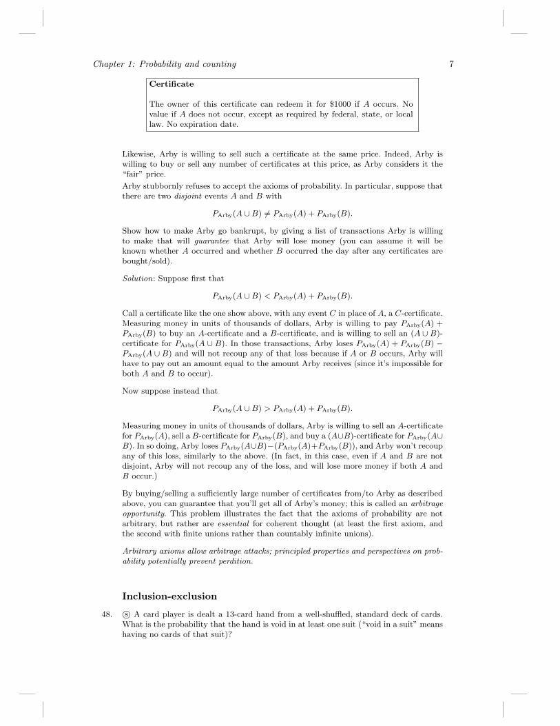
Certificate
The owner of this certificate can redeem it for $1000 if A occurs. Novalue if A does not occur, except as required by federal, state, or locallaw. No expiration date.
Likewise, Arby is willing to sell such a certificate at the same price. Indeed, Arby iswilling to buy or sell any number of certificates at this price, as Arby considers it the“fair” price.
Arby stubbornly refuses to accept the axioms of probability. In particular, suppose thatthere are two disjoint events A and B with
PArby(A ∪B) 6= PArby(A) + PArby(B).
Show how to make Arby go bankrupt, by giving a list of transactions Arby is willingto make that will guarantee that Arby will lose money (you can assume it will beknown whether A occurred and whether B occurred the day after any certificates arebought/sold).
Solution: Suppose first that
PArby(A ∪B) < PArby(A) + PArby(B).
Call a certificate like the one show above, with any event C in place of A, a C-certificate.Measuring money in units of thousands of dollars, Arby is willing to pay PArby(A) +PArby(B) to buy an A-certificate and a B-certificate, and is willing to sell an (A ∪ B)-certificate for PArby(A ∪ B). In those transactions, Arby loses PArby(A) + PArby(B) −PArby(A ∪ B) and will not recoup any of that loss because if A or B occurs, Arby willhave to pay out an amount equal to the amount Arby receives (since it’s impossible forboth A and B to occur).
Now suppose instead that
PArby(A ∪B) > PArby(A) + PArby(B).
Measuring money in units of thousands of dollars, Arby is willing to sell an A-certificatefor PArby(A), sell a B-certificate for PArby(B), and buy a (A∪B)-certificate for PArby(A∪B). In so doing, Arby loses PArby(A∪B)−(PArby(A)+PArby(B)), and Arby won’t recoupany of this loss, similarly to the above. (In fact, in this case, even if A and B are notdisjoint, Arby will not recoup any of the loss, and will lose more money if both A andB occur.)
By buying/selling a sufficiently large number of certificates from/to Arby as describedabove, you can guarantee that you’ll get all of Arby’s money; this is called an arbitrageopportunity. This problem illustrates the fact that the axioms of probability are notarbitrary, but rather are essential for coherent thought (at least the first axiom, andthe second with finite unions rather than countably infinite unions).
Arbitrary axioms allow arbitrage attacks; principled properties and perspectives on prob-ability potentially prevent perdition.
Inclusion-exclusion
48. s© A card player is dealt a 13-card hand from a well-shuffled, standard deck of cards.What is the probability that the hand is void in at least one suit (“void in a suit” meanshaving no cards of that suit)?
8 Chapter 1: Probability and counting
Solution: Let S,H,D,C be the events of being void in Spades, Hearts, Diamonds, Clubs,respectively. We want to find P (S ∪D ∪H ∪C). By inclusion-exclusion and symmetry,
P (S ∪D ∪H ∪ C) = 4P (S)− 6P (S ∩H) + 4P (S ∩H ∩D)− P (S ∩H ∩D ∩ C).
The probability of being void in a specific suit is(3913)(5213)
. The probability of being void in
2 specific suits is(2613)(5213)
. The probability of being void in 3 specific suits is 1
(5213). And the
last term is 0 since it’s impossible to be void in everything. So the probability is
4
(3913
)(5213
) − 6
(2613
)(5213
) +4(5213
) ≈ 0.051.
52. s© Alice attends a small college in which each class meets only once a week. She isdeciding between 30 non-overlapping classes. There are 6 classes to choose from for eachday of the week, Monday through Friday. Trusting in the benevolence of randomness,Alice decides to register for 7 randomly selected classes out of the 30, with all choicesequally likely. What is the probability that she will have classes every day, Mondaythrough Friday? (This problem can be done either directly using the naive definition ofprobability, or using inclusion-exclusion.)
Solution: We will solve this both by direct counting and using inclusion-exclusion.
Direct Counting Method : There are two general ways that Alice can have class everyday: either she has 2 days with 2 classes and 3 days with 1 class, or she has 1 day with 3classes, and has 1 class on each of the other 4 days. The number of possibilities for the
former is(52
)(62
)263 (choose the 2 days when she has 2 classes, and then select 2 classes
on those days and 1 class for the other days). The number of possibilities for the latteris(51
)(63
)64. So the probability is(
52
)(62
)263 +
(51
)(63
)64(
307
) =114
377≈ 0.302.
Inclusion-Exclusion Method : We will use inclusion-exclusion to find the probability ofthe complement, which is the event that she has at least one day with no classes. LetBi = Aci . Then
P (B1 ∪B2 · · · ∪B5) =∑i
P (Bi)−∑i<j
P (Bi ∩Bj) +∑i<j<k
P (Bi ∩Bj ∩Bk)
(terms with the intersection of 4 or more Bi’s are not needed since Alice must haveclasses on at least 2 days). We have
P (B1) =
(247
)(307
) , P (B1 ∩B2) =
(187
)(307
) , P (B1 ∩B2 ∩B3) =
(127
)(307
)and similarly for the other intersections. So
P (B1 ∪ · · · ∪B5) = 5
(247
)(307
) −(5
2
)(187
)(307
) +
(5
3
)(127
)(307
) =263
377.
Therefore,
P (A1 ∩A2 ∩A3 ∩A4 ∩A5) =114
377≈ 0.302.
Chapter 1: Probability and counting 9
Mixed practice
59. s© There are 100 passengers lined up to board an airplane with 100 seats (with eachseat assigned to one of the passengers). The first passenger in line crazily decides tosit in a randomly chosen seat (with all seats equally likely). Each subsequent passengertakes his or her assigned seat if available, and otherwise sits in a random available seat.What is the probability that the last passenger in line gets to sit in his or her assignedseat? (This is a common interview problem, and a beautiful example of the power ofsymmetry.)
Hint: Call the seat assigned to the jth passenger in line “seat j” (regardless of whetherthe airline calls it seat 23A or whatever). What are the possibilities for which seatsare available to the last passenger in line, and what is the probability of each of thesepossibilities?
Solution: The seat for the last passenger is either seat 1 or seat 100; for example, seat42 can’t be available to the last passenger since the 42nd passenger in line would havesat there if possible. Seat 1 and seat 100 are equally likely to be available to the lastpassenger, since the previous 99 passengers view these two seats symmetrically. So theprobability that the last passenger gets seat 100 is 1/2.

Chapter 2: Conditional probability
Conditioning on evidence
1. s© A spam filter is designed by looking at commonly occurring phrases in spam. Supposethat 80% of email is spam. In 10% of the spam emails, the phrase “free money” is used,whereas this phrase is only used in 1% of non-spam emails. A new email has just arrived,which does mention “free money”. What is the probability that it is spam?
Solution: Let S be the event that an email is spam and F be the event that an emailhas the “free money” phrase. By Bayes’ rule,
P (S|F ) =P (F |S)P (S)
P (F )=
0.1 · 0.80.1 · 0.8 + 0.01 · 0.2 =
80/1000
82/1000=
80
82≈ 0.9756.
2. s© A woman is pregnant with twin boys. Twins may be either identical or fraternal (non-identical). In general, 1/3 of twins born are identical. Obviously, identical twins mustbe of the same sex; fraternal twins may or may not be. Assume that identical twins areequally likely to be both boys or both girls, while for fraternal twins all possibilities areequally likely. Given the above information, what is the probability that the woman’stwins are identical?
Solution: By Bayes’ rule,
P (identical|BB) =P (BB|identical)P (identical)
P (BB)=
12· 13
12· 13
+ 14· 23
= 1/2.
22. s© A bag contains one marble which is either green or blue, with equal probabilities. Agreen marble is put in the bag (so there are 2 marbles now), and then a random marbleis taken out. The marble taken out is green. What is the probability that the remainingmarble is also green?
Solution: Let A be the event that the initial marble is green, B be the event that theremoved marble is green, and C be the event that the remaining marble is green. Weneed to find P (C|B). There are several ways to find this; one natural way is to conditionon whether the initial marble is green:
P (C|B) = P (C|B,A)P (A|B) + P (C|B,Ac)P (Ac|B) = 1P (A|B) + 0P (Ac|B).
To find P (A|B), use Bayes’ Rule:
P (A|B) =P (B|A)P (A)
P (B)=
1/2
P (B|A)P (A) + P (B|Ac)P (Ac)=
1/2
1/2 + 1/4=
2
3.
So P (C|B) = 2/3.
Historical note: This problem was first posed by Lewis Carroll in 1893.
23. s© Let G be the event that a certain individual is guilty of a certain robbery. In gatheringevidence, it is learned that an event E1 occurred, and a little later it is also learned thatanother event E2 also occurred. Is it possible that individually, these pieces of evidence
11
12 Chapter 2: Conditional probability
increase the chance of guilt (so P (G|E1) > P (G) and P (G|E2) > P (G)), but togetherthey decrease the chance of guilt (so P (G|E1, E2) < P (G))?
Solution: Yes, this is possible. In fact, it is possible to have two events which separatelyprovide evidence in favor of G, yet which together preclude G! For example, supposethat the crime was committed between 1 pm and 3 pm on a certain day. Let E1 bethe event that the suspect was at a specific nearby coffeeshop from 1 pm to 2 pm thatday, and let E2 be the event that the suspect was at the nearby coffeeshop from 2 pmto 3 pm that day. Then P (G|E1) > P (G), P (G|E2) > P (G) (assuming that being inthe vicinity helps show that the suspect had the opportunity to commit the crime), yetP (G|E1 ∩E2) < P (G) (as being in the coffeehouse from 1 pm to 3 pm gives the suspectan alibi for the full time).
25. s© A crime is committed by one of two suspects, A and B. Initially, there is equalevidence against both of them. In further investigation at the crime scene, it is foundthat the guilty party had a blood type found in 10% of the population. Suspect A doesmatch this blood type, whereas the blood type of Suspect B is unknown.
(a) Given this new information, what is the probability that A is the guilty party?
(b) Given this new information, what is the probability that B’s blood type matchesthat found at the crime scene?
Solution:
(a) Let M be the event that A’s blood type matches the guilty party’s and for brevity,write A for “A is guilty” and B for “B is guilty”. By Bayes’ Rule,
P (A|M) =P (M |A)P (A)
P (M |A)P (A) + P (M |B)P (B)=
1/2
1/2 + (1/10)(1/2)=
10
11.
(We have P (M |B) = 1/10 since, given that B is guilty, the probability that A’s bloodtype matches the guilty party’s is the same probability as for the general population.)
(b) Let C be the event that B’s blood type matches, and condition on whether B isguilty. This gives
P (C|M) = P (C|M,A)P (A|M) + P (C|M,B)P (B|M) =1
10· 10
11+
1
11=
2
11.
26. s© To battle against spam, Bob installs two anti-spam programs. An email arrives,which is either legitimate (event L) or spam (event Lc), and which program j marks aslegitimate (event Mj) or marks as spam (event Mc
j ) for j ∈ {1, 2}. Assume that 10%of Bob’s email is legitimate and that the two programs are each “90% accurate” in thesense that P (Mj |L) = P (Mc
j |Lc) = 9/10. Also assume that given whether an email isspam, the two programs’ outputs are conditionally independent.
(a) Find the probability that the email is legitimate, given that the 1st program marksit as legitimate (simplify).
(b) Find the probability that the email is legitimate, given that both programs mark itas legitimate (simplify).
(c) Bob runs the 1st program and M1 occurs. He updates his probabilities and thenruns the 2nd program. Let P (A) = P (A|M1) be the updated probability function afterrunning the 1st program. Explain briefly in words whether or not P (L|M2) = P (L|M1∩M2): is conditioning on M1∩M2 in one step equivalent to first conditioning on M1, thenupdating probabilities, and then conditioning on M2?
Solution:
Chapter 2: Conditional probability 13
(a) By Bayes’ rule,
P (L|M1) =P (M1|L)P (L)
P (M1)=
910· 110
910· 110
+ 110· 910
=1
2.
(b) By Bayes’ rule,
P (L|M1,M2) =P (M1,M2|L)P (L)
P (M1,M2)=
( 910
)2 · 110
( 910
)2 · 110
+ ( 110
)2 · 910
=9
10.
(c) Yes, they are the same, since Bayes’ rule is coherent. The probability of an eventgiven various pieces of evidence does not depend on the order in which the pieces ofevidence are incorporated into the updated probabilities.
Independence and conditional independence
30. s© A family has 3 children, creatively named A,B, and C.
(a) Discuss intuitively (but clearly) whether the event “A is older than B” is independentof the event “A is older than C”.
(b) Find the probability that A is older than B, given that A is older than C.
Solution:
(a) They are not independent: knowing that A is older than B makes it more likely thatA is older than C, as the if A is older than B, then the only way that A can be youngerthan C is if the birth order is CAB, whereas the birth orders ABC and ACB are bothcompatible with A being older than B. To make this more intuitive, think of an extremecase where there are 100 children instead of 3, call them A1, . . . , A100. Given that A1
is older than all of A2, A3, . . . , A99, it’s clear that A1 is very old (relatively), whereasthere isn’t evidence about where A100 fits into the birth order.
(b) Writing x > y to mean that x is older than y,
P (A > B|A > C) =P (A > B,A > C)
P (A > C)=
1/3
1/2=
2
3
since P (A > B,A > C) = P (A is the eldest child) = 1/3 (unconditionally, any of the 3children is equally likely to be the eldest).
31. s© Is it possible that an event is independent of itself? If so, when is this the case?
Solution: LetA be an event. IfA is independent of itself, then P (A) = P (A∩A) = P (A)2,so P (A) is 0 or 1. So this is only possible in the extreme cases that the event hasprobability 0 or 1.
32. s© Consider four nonstandard dice (the Efron dice), whose sides are labeled as follows(the 6 sides on each die are equally likely).
A: 4, 4, 4, 4, 0, 0
B: 3, 3, 3, 3, 3, 3
C: 6, 6, 2, 2, 2, 2
D: 5, 5, 5, 1, 1, 1
These four dice are each rolled once. Let A be the result for die A, B be the result fordie B, etc.
14 Chapter 2: Conditional probability
(a) Find P (A > B), P (B > C), P (C > D), and P (D > A).
(b) Is the event A > B independent of the event B > C? Is the event B > C independentof the event C > D? Explain.
Solution:
(a)P (A > B) = P (A = 4) = 2/3
P (B > C) = P (C = 2) = 2/3
P (C > D) = P (C = 6) + P (C = 2, D = 1) = 2/3
P (D > A) = P (D = 5) + P (D = 1, A = 0) = 2/3
(b) The event A > B is independent of the event B > C since A > B is the samething as A = 4, knowledge of which gives no information about B > C (which is thesame thing as C = 2). On the other hand, B > C is not independent of C > D sinceP (C > D|C = 2) = 1/2 6= 1 = P (C > D|C 6= 2).
35. s© You are going to play 2 games of chess with an opponent whom you have neverplayed against before (for the sake of this problem). Your opponent is equally likely tobe a beginner, intermediate, or a master. Depending on which, your chances of winningan individual game are 90%, 50%, or 30%, respectively.
(a) What is your probability of winning the first game?
(b) Congratulations: you won the first game! Given this information, what is the prob-ability that you will also win the second game (assume that, given the skill level of youropponent, the outcomes of the games are independent)?
(c) Explain the distinction between assuming that the outcomes of the games are in-dependent and assuming that they are conditionally independent given the opponent’sskill level. Which of these assumptions seems more reasonable, and why?
Solution:
(a) Let Wi be the event of winning the ith game. By the law of total probability,
P (W1) = (0.9 + 0.5 + 0.3)/3 = 17/30.
(b) We have P (W2|W1) = P (W2,W1)/P (W1). The denominator is known from (a),while the numerator can be found by conditioning on the skill level of the opponent:
P (W1,W2) =1
3P (W1,W2|beginner)+
1
3P (W1,W2|intermediate)+
1
3P (W1,W2|expert).
Since W1 and W2 are conditionally independent given the skill level of the opponent,this becomes
P (W1,W2) = (0.92 + 0.52 + 0.32)/3 = 23/60.
So
P (W2|W1) =23/60
17/30= 23/34.
(c) Independence here means that knowing one game’s outcome gives no informationabout the other game’s outcome, while conditional independence is the same statementwhere all probabilities are conditional on the opponent’s skill level. Conditional inde-pendence given the opponent’s skill level is a more reasonable assumption here. This isbecause winning the first game gives information about the opponent’s skill level, whichin turn gives information about the result of the second game.
That is, if the opponent’s skill level is treated as fixed and known, then it may bereasonable to assume independence of games given this information; with the opponent’sskill level random, earlier games can be used to help infer the opponent’s skill level, whichaffects the probabilities for future games.
Chapter 2: Conditional probability 15
Monty Hall
38. s© (a) Consider the following 7-door version of the Monty Hall problem. There are 7doors, behind one of which there is a car (which you want), and behind the rest of whichthere are goats (which you don’t want). Initially, all possibilities are equally likely forwhere the car is. You choose a door. Monty Hall then opens 3 goat doors, and offersyou the option of switching to any of the remaining 3 doors.
Assume that Monty Hall knows which door has the car, will always open 3 goat doorsand offer the option of switching, and that Monty chooses with equal probabilities fromall his choices of which goat doors to open. Should you switch? What is your probabilityof success if you switch to one of the remaining 3 doors?
(b) Generalize the above to a Monty Hall problem where there are n ≥ 3 doors, of whichMonty opens m goat doors, with 1 ≤ m ≤ n− 2.
Solution:
(a) Assume the doors are labeled such that you choose door 1 (to simplify notation),and suppose first that you follow the “stick to your original choice” strategy. Let S bethe event of success in getting the car, and let Cj be the event that the car is behinddoor j. Conditioning on which door has the car, we have
P (S) = P (S|C1)P (C1) + · · ·+ P (S|C7)P (C7) = P (C1) =1
7.
Let Mijk be the event that Monty opens doors i, j, k. Then
P (S) =∑i,j,k
P (S|Mijk)P (Mijk)
(summed over all i, j, k with 2 ≤ i < j < k ≤ 7.) By symmetry, this gives
P (S|Mijk) = P (S) =1
7
for all i, j, k with 2 ≤ i < j < k ≤ 7. Thus, the conditional probability that the car isbehind 1 of the remaining 3 doors is 6/7, which gives 2/7 for each. So you should switch,thus making your probability of success 2/7 rather than 1/7.
(b) By the same reasoning, the probability of success for “stick to your original choice”is 1
n, both unconditionally and conditionally. Each of the n − m − 1 remaining doors
has conditional probability n−1(n−m−1)n
of having the car. This value is greater than 1n
, so
you should switch, thus obtaining probability n−1(n−m−1)n
of success (both conditionally
and unconditionally).
39. s© Consider the Monty Hall problem, except that Monty enjoys opening door 2 morethan he enjoys opening door 3, and if he has a choice between opening these two doors,he opens door 2 with probability p, where 1
2≤ p ≤ 1.
To recap: there are three doors, behind one of which there is a car (which you want),and behind the other two of which there are goats (which you don’t want). Initially,all possibilities are equally likely for where the car is. You choose a door, which forconcreteness we assume is door 1. Monty Hall then opens a door to reveal a goat, andoffers you the option of switching. Assume that Monty Hall knows which door has thecar, will always open a goat door and offer the option of switching, and as above assumethat if Monty Hall has a choice between opening door 2 and door 3, he chooses door 2with probability p (with 1
2≤ p ≤ 1).
(a) Find the unconditional probability that the strategy of always switching succeeds(unconditional in the sense that we do not condition on which of doors 2 or 3 Montyopens).
16 Chapter 2: Conditional probability
(b) Find the probability that the strategy of always switching succeeds, given that Montyopens door 2.
(c) Find the probability that the strategy of always switching succeeds, given that Montyopens door 3.
Solution:
(a) Let Cj be the event that the car is hidden behind door j and let W be the eventthat we win using the switching strategy. Using the law of total probability, we can findthe unconditional probability of winning:
P (W ) = P (W |C1)P (C1) + P (W |C2)P (C2) + P (W |C3)P (C3)
= 0 · 1/3 + 1 · 1/3 + 1 · 1/3 = 2/3.
(b) A tree method works well here (delete the paths which are no longer relevant afterthe conditioning, and reweight the remaining values by dividing by their sum), or wecan use Bayes’ rule and the law of total probability (as below).
Let Di be the event that Monty opens Door i. Note that we are looking for P (W |D2),which is the same as P (C3|D2) as we first choose Door 1 and then switch to Door 3. ByBayes’ rule and the law of total probability,
P (C3|D2) =P (D2|C3)P (C3)
P (D2)
=P (D2|C3)P (C3)
P (D2|C1)P (C1) + P (D2|C2)P (C2) + P (D2|C3)P (C3)
=1 · 1/3
p · 1/3 + 0 · 1/3 + 1 · 1/3
=1
1 + p.
(c) The structure of the problem is the same as part (b) (except for the condition thatp ≥ 1/2, which was not needed above). Imagine repainting doors 2 and 3, reversingwhich is called which. By part (b) with 1− p in place of p, P (C2|D3) = 1
1+(1−p) = 12−p .
First-step analysis and gambler’s ruin
42. s© A fair die is rolled repeatedly, and a running total is kept (which is, at each time,the total of all the rolls up until that time). Let pn be the probability that the runningtotal is ever exactly n (assume the die will always be rolled enough times so that therunning total will eventually exceed n, but it may or may not ever equal n).
(a) Write down a recursive equation for pn (relating pn to earlier terms pk in a simpleway). Your equation should be true for all positive integers n, so give a definition of p0and pk for k < 0 so that the recursive equation is true for small values of n.
(b) Find p7.
(c) Give an intuitive explanation for the fact that pn → 1/3.5 = 2/7 as n→∞.
Solution:
(a) We will find something to condition on to reduce the case of interest to earlier,simpler cases. This is achieved by the useful strategy of first step anaysis. Let pn be theprobability that the running total is ever exactly n. Note that if, for example, the first

Chapter 2: Conditional probability 17
throw is a 3, then the probability of reaching n exactly is pn−3 since starting from thatpoint, we need to get a total of n− 3 exactly. So
pn =1
6(pn−1 + pn−2 + pn−3 + pn−4 + pn−5 + pn−6),
where we define p0 = 1 (which makes sense anyway since the running total is 0 beforethe first toss) and pk = 0 for k < 0.
(b) Using the recursive equation in (a), we have
p1 =1
6, p2 =
1
6(1 +
1
6), p3 =
1
6(1 +
1
6)2,
p4 =1
6(1 +
1
6)3, p5 =
1
6(1 +
1
6)4, p6 =
1
6(1 +
1
6)5.
Hence,
p7 =1
6(p1 + p2 + p3 + p4 + p5 + p6) =
1
6
((1 +
1
6)6 − 1
)≈ 0.2536.
(c) An intuitive explanation is as follows. The average number thrown by the die is(total of dots)/6, which is 21/6 = 7/2, so that every throw adds on an average of 7/2.We can therefore expect to land on 2 out of every 7 numbers, and the probability oflanding on any particular number is 2/7. A mathematical derivation (which was notrequested in the problem) can be given as follows:
pn+1 + 2pn+2 + 3pn+3 + 4pn+4 + 5pn+5 + 6pn+6
=pn+1 + 2pn+2 + 3pn+3 + 4pn+4 + 5pn+5
+ pn + pn+1 + pn+2 + pn+3 + pn+4 + pn+5
=pn + 2pn+1 + 3pn+2 + 4pn+3 + 5pn+4 + 6pn+5
= · · ·=p−5 + 2p−4 + 3p−3 + 4p−2 + 5p−1 + 6p0 = 6.
Taking the limit of the lefthand side as n goes to ∞, we have
(1 + 2 + 3 + 4 + 5 + 6) limn→∞
pn = 6,
so limn→∞ pn = 2/7.
44. s© Calvin and Hobbes play a match consisting of a series of games, where Calvin hasprobability p of winning each game (independently). They play with a “win by two””rule: the first player to win two games more than his opponent wins the match. Findthe probability that Calvin wins the match (in terms of p), in two different ways:
(a) by conditioning, using the law of total probability.
(b) by interpreting the problem as a gambler’s ruin problem.
Solution:
(a) Let C be the event that Calvin wins the match, X ∼ Bin(2, p) be how many of thefirst 2 games he wins, and q = 1− p. Then
P (C) = P (C|X = 0)q2 + P (C|X = 1)(2pq) + P (C|X = 2)p2 = 2pqP (C) + p2,
so P (C) = p2
1−2pq. This can also be written as p2
p2+q2, since p+ q = 1.
Sanity check : Note that this should (and does) reduce to 1 for p = 1, 0 for p = 0, and
18 Chapter 2: Conditional probability
12
for p = 12. Also, it makes sense that the probability of Hobbes winning, which is
1− P (C) = q2
p2+q2, can also be obtained by swapping p and q.
(b) The problem can be thought of as a gambler’s ruin where each player starts outwith $2. So the probability that Calvin wins the match is
1− (q/p)2
1− (q/p)4=
(p2 − q2)/p2
(p4 − q4)/p4=
(p2 − q2)/p2
(p2 − q2)(p2 + q2)/p4=
p2
p2 + q2,
which agrees with the above.
Simpson’s paradox
49. s© (a) Is it possible to have events A,B,C such that P (A|C) < P (B|C) and P (A|Cc) <P (B|Cc), yet P (A) > P (B)? That is, A is less likely than B given that C is true,and also less likely than B given that C is false, yet A is more likely than B if we’regiven no information about C. Show this is impossible (with a short proof) or find acounterexample (with a story interpreting A,B,C).
(b) If the scenario in (a) is possible, is it a special case of Simpson’s paradox, equivalent toSimpson’s paradox, or neither? If it is impossible, explain intuitively why it is impossibleeven though Simpson’s paradox is possible.
Solution:
(a) It is not possible, as seen using the law of total probability:
P (A) = P (A|C)P (C) + P (A|Cc)P (Cc) < P (B|C)P (C) + P (B|Cc)P (Cc) = P (B).
(b) In Simpson’s paradox, using the notation from the chapter, we can expand outP (A|B) and P (A|Bc) using LOTP to condition on C, but the inequality can flip becauseof the weights such as P (C|B) on the terms (e.g., Dr. Nick performs a lot more Band-Aid removals than Dr. Hibbert). In this problem, the weights P (C) and P (Cc) are thesame in both expansions, so the inequality is preserved.
50. s© Consider the following conversation from an episode of The Simpsons:
Lisa: Dad, I think he’s an ivory dealer! His boots are ivory, his hat isivory, and I’m pretty sure that check is ivory.
Homer: Lisa, a guy who has lots of ivory is less likely to hurt Stampythan a guy whose ivory supplies are low.
Here Homer and Lisa are debating the question of whether or not the man (namedBlackheart) is likely to hurt Stampy the Elephant if they sell Stampy to him. Theyclearly disagree about how to use their observations about Blackheart to learn aboutthe probability (conditional on the evidence) that Blackheart will hurt Stampy.
(a) Define clear notation for the various events of interest here.
(b) Express Lisa’s and Homer’s arguments (Lisa’s is partly implicit) as conditionalprobability statements in terms of your notation from (a).
(c) Assume it is true that someone who has a lot of a commodity will have less desireto acquire more of the commodity. Explain what is wrong with Homer’s reasoning thatthe evidence about Blackheart makes it less likely that he will harm Stampy.
Solution:
(a) Let H be the event that the man will hurt Stampy, let L be the event that a manhas lots of ivory, and let D be the event that the man is an ivory dealer.
Chapter 2: Conditional probability 19
(b) Lisa observes that L is true. She suggests (reasonably) that this evidence makes Dmore likely, i.e., P (D|L) > P (D). Implicitly, she suggests that this makes it likely thatthe man will hurt Stampy, i.e.,
P (H|L) > P (H|Lc).
Homer argues thatP (H|L) < P (H|Lc).
(c) Homer does not realize that observing that Blackheart has so much ivory makesit much more likely that Blackheart is an ivory dealer, which in turn makes it morelikely that the man will hurt Stampy. This is an example of Simpson’s paradox. It maybe true that, controlling for whether or not Blackheart is a dealer, having high ivorysupplies makes it less likely that he will harm Stampy: P (H|L,D) < P (H|Lc, D) andP (H|L,Dc) < P (H|Lc, Dc). However, this does not imply that P (H|L) < P (H|Lc).
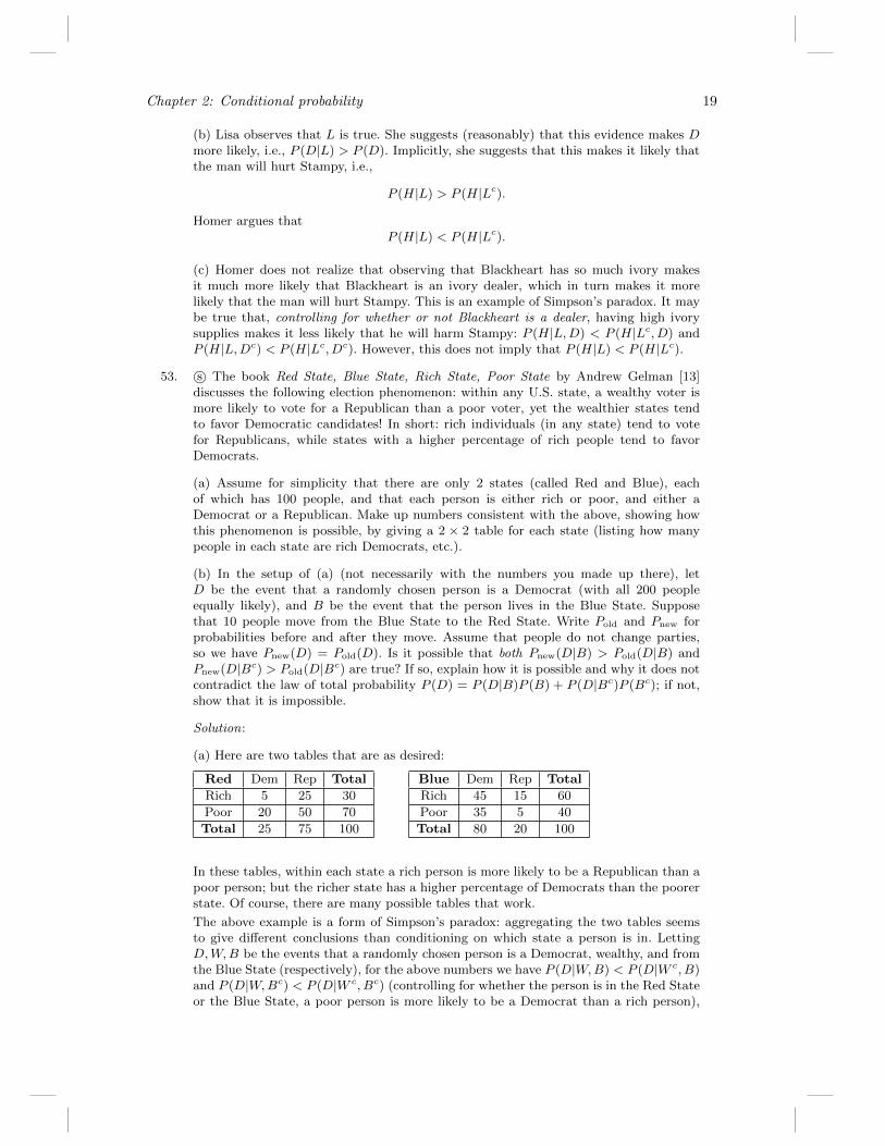
53. s© The book Red State, Blue State, Rich State, Poor State by Andrew Gelman [13]discusses the following election phenomenon: within any U.S. state, a wealthy voter ismore likely to vote for a Republican than a poor voter, yet the wealthier states tendto favor Democratic candidates! In short: rich individuals (in any state) tend to votefor Republicans, while states with a higher percentage of rich people tend to favorDemocrats.
(a) Assume for simplicity that there are only 2 states (called Red and Blue), eachof which has 100 people, and that each person is either rich or poor, and either aDemocrat or a Republican. Make up numbers consistent with the above, showing howthis phenomenon is possible, by giving a 2 × 2 table for each state (listing how manypeople in each state are rich Democrats, etc.).
(b) In the setup of (a) (not necessarily with the numbers you made up there), letD be the event that a randomly chosen person is a Democrat (with all 200 peopleequally likely), and B be the event that the person lives in the Blue State. Supposethat 10 people move from the Blue State to the Red State. Write Pold and Pnew forprobabilities before and after they move. Assume that people do not change parties,so we have Pnew(D) = Pold(D). Is it possible that both Pnew(D|B) > Pold(D|B) andPnew(D|Bc) > Pold(D|Bc) are true? If so, explain how it is possible and why it does notcontradict the law of total probability P (D) = P (D|B)P (B) + P (D|Bc)P (Bc); if not,show that it is impossible.
Solution:
(a) Here are two tables that are as desired:
Red Dem Rep Total
Rich 5 25 30
Poor 20 50 70
Total 25 75 100
Blue Dem Rep Total
Rich 45 15 60
Poor 35 5 40
Total 80 20 100
In these tables, within each state a rich person is more likely to be a Republican than apoor person; but the richer state has a higher percentage of Democrats than the poorerstate. Of course, there are many possible tables that work.
The above example is a form of Simpson’s paradox: aggregating the two tables seemsto give different conclusions than conditioning on which state a person is in. LettingD,W,B be the events that a randomly chosen person is a Democrat, wealthy, and fromthe Blue State (respectively), for the above numbers we have P (D|W,B) < P (D|W c, B)and P (D|W,Bc) < P (D|W c, Bc) (controlling for whether the person is in the Red Stateor the Blue State, a poor person is more likely to be a Democrat than a rich person),
20 Chapter 2: Conditional probability
but P (D|W ) > P (D|W c) (stemming from the fact that the Blue State is richer andmore Democratic).
(b) Yes, it is possible. Suppose with the numbers from (a) that 10 people move from theBlue State to the Red State, of whom 5 are Democrats and 5 are Republicans. ThenPnew(D|B) = 75/90 > 80/100 = Pold(D|B) and Pnew(D|Bc) = 30/110 > 25/100 =Pold(D|Bc). Intuitively, this makes sense since the Blue State has a higher percentageof Democrats initially than the Red State, and the people who move have a percentageof Democrats which is between these two values.
This result does not contradict the law of total probability since the weights P (B), P (Bc)also change: Pnew(B) = 90/200, while Pold(B) = 1/2. The phenomenon could not occurif an equal number of people also move from the Red State to the Blue State (so thatP (B) is kept constant).
Chapter 3: Random variables and theirdistributions
PMFs and CDFs
6. s© Benford’s law states that in a very large variety of real-life data sets, the first digitapproximately follows a particular distribution with about a 30% chance of a 1, an 18%chance of a 2, and in general
P (D = j) = log10
(j + 1
j
), for j ∈ {1, 2, 3, . . . , 9},
where D is the first digit of a randomly chosen element. Check that this is a valid PMF(using properties of logs, not with a calculator).
Solution: The function P (D = j) is nonnegative and the sum over all values is
9∑j=1
log10
j + 1
j=
9∑j=1
(log10(j + 1)− log10(j)).
All terms cancel except log10 10 − log10 1 = 1 (this is a telescoping series). Since thevalues add to 1 and are nonnegative, P (D = j) is a PMF.
11. s© Let X be an r.v. whose possible values are 0, 1, 2, . . . , with CDF F . In some countries,rather than using a CDF, the convention is to use the function G defined by G(x) =P (X < x) to specify a distribution. Find a way to convert from F to G, i.e., if F is aknown function, show how to obtain G(x) for all real x.
Solution: Write
G(x) = P (X ≤ x)− P (X = x) = F (x)− P (X = x).
If x is not a nonnegative integer, then P (X = x) = 0 so G(x) = F (x). For x a nonneg-ative integer,
P (X = x) = F (x)− F (x− 1/2)
since the PMF corresponds to the lengths of the jumps in the CDF. (The 1/2 was chosenfor concreteness; we also have F (x− 1/2) = F (x− a) for any a ∈ (0, 1].) Thus,
G(x) =
{F (x) if x /∈ {0, 1, 2, . . . }F (x− 1/2) if x ∈ {0, 1, 2, . . . }.
More compactly, we can also write G(x) = limt→x− F (t), where the − denotes takinga limit from the left (recall that F is right continuous), and G(x) = F (dxe − 1), wheredxe is the ceiling of x (the smallest integer greater than or equal to x).
Named distributions
18. s© (a) In the World Series of baseball, two teams (call them A and B) play a sequenceof games against each other, and the first team to win four games wins the series. Let
21
22 Chapter 3: Random variables and their distributions
p be the probability that A wins an individual game, and assume that the games areindependent. What is the probability that team A wins the series?
(b) Give a clear intuitive explanation of whether the answer to (a) depends on whetherthe teams always play 7 games (and whoever wins the majority wins the series), or theteams stop playing more games as soon as one team has won 4 games (as is actuallythe case in practice: once the match is decided, the two teams do not keep playing moregames).
Solution:
(a) Let q = 1− p. First let us do a direct calculation:
P (A wins) = P (A wins in 4 games) + P (A wins in 5 games)
+P (A wins in 6 games) + P (A wins in 7 games)
= p4 +
(4
3
)p4q +
(5
3
)p4q2 +
(6
3
)p4q3.
To understand how these probabilities are calculated, note for example that
P (A wins in 5) = P (A wins 3 out of first 4) · P (A wins 5th game|A wins 3 out of first 4)
=
(4
3
)p3qp.
(Each of the 4 terms in the expression for P (A wins) can also be found using the PMFof a distribution known as the Negative Binomial, which is introduced in Chapter 4.)
An neater solution is to use the fact (explained in the solution to Part (b)) that we canassume that the teams play all 7 games no matter what. Let X be the number of winsfor team A, so that X ∼ Bin(7, p). Then
P (X ≥ 4) = P (X = 4) + P (X = 5) + P (X = 6) + P (X = 7)
=
(7
4
)p4q3 +
(7
5
)p5q2 +
(7
6
)p6q + p7,
which looks different from the above but is actually identical as a function of p (as canbe verified by simplifying both expressions as polynomials in p).
(b) The answer to (a) does not depend on whether the teams play all seven games nomatter what. Imagine telling the players to continue playing the games even after thematch has been decided, just for fun: the outcome of the match won’t be affected bythis, and this also means that the probability that A wins the match won’t be affectedby assuming that the teams always play 7 games!
21. s© Let X ∼ Bin(n, p) and Y ∼ Bin(m, p), independent of X. Show that X − Y is notBinomial.
Solution: A Binomial can’t be negative, but X−Y is negative with positive probability.
25. s© Alice flips a fair coin n times and Bob flips another fair coin n + 1 times, resultingin independent X ∼ Bin(n, 1
2) and Y ∼ Bin(n+ 1, 1
2).
(a) Show that P (X < Y ) = P (n−X < n+ 1− Y ).
(b) Compute P (X < Y ).
Hint: Use (a) and the fact that X and Y are integer-valued.
Solution:
Chapter 3: Random variables and their distributions 23
(a) Note that n−X ∼ Bin(n, 1/2) and n+1−Y ∼ Bin(n+1, 1/2) (we can interpret thisby thinking of counting Tails rather than counting Heads), with n −X and n + 1 − Yindependent. So P (X < Y ) = P (n−X < n+ 1− Y ), since both sides have exactly thesame structure.
(b) We have
P (X < Y ) = P (n−X < n+ 1− Y ) = P (Y < X + 1) = P (Y ≤ X)
since X and Y are integer-valued (e.g., Y < 5 is equivalent to Y ≤ 4). But Y ≤ X isthe complement of X < Y , so P (X < Y ) = 1− P (X < Y ). Thus, P (X < Y ) = 1/2.
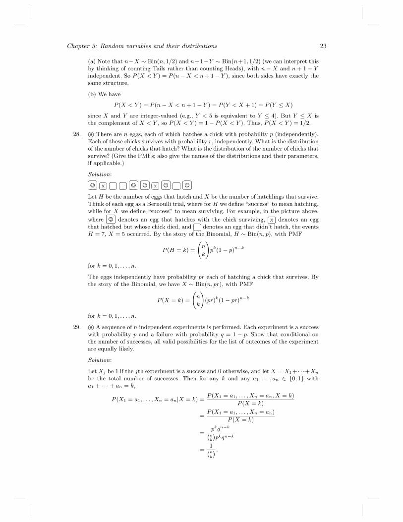
28. s© There are n eggs, each of which hatches a chick with probability p (independently).Each of these chicks survives with probability r, independently. What is the distributionof the number of chicks that hatch? What is the distribution of the number of chicks thatsurvive? (Give the PMFs; also give the names of the distributions and their parameters,if applicable.)
Solution:�� ��©�� ��x
�� ���� ���� ��©�� ��©
�� ��x�� ��©
�� ���� ��©
Let H be the number of eggs that hatch and X be the number of hatchlings that survive.Think of each egg as a Bernoulli trial, where for H we define “success” to mean hatching,while for X we define “success” to mean surviving. For example, in the picture above,
where�� ��© denotes an egg that hatches with the chick surviving,
�� ��x denotes an eggthat hatched but whose chick died, and
�� ��denotes an egg that didn’t hatch, the eventsH = 7, X = 5 occurred. By the story of the Binomial, H ∼ Bin(n, p), with PMF
P (H = k) =
(n
k
)pk(1− p)n−k
for k = 0, 1, . . . , n.
The eggs independently have probability pr each of hatching a chick that survives. Bythe story of the Binomial, we have X ∼ Bin(n, pr), with PMF
P (X = k) =
(n
k
)(pr)k(1− pr)n−k
for k = 0, 1, . . . , n.
29. s© A sequence of n independent experiments is performed. Each experiment is a successwith probability p and a failure with probability q = 1 − p. Show that conditional onthe number of successes, all valid possibilities for the list of outcomes of the experimentare equally likely.
Solution:
Let Xj be 1 if the jth experiment is a success and 0 otherwise, and let X = X1+· · ·+Xnbe the total number of successes. Then for any k and any a1, . . . , an ∈ {0, 1} witha1 + · · ·+ an = k,
P (X1 = a1, . . . , Xn = an|X = k) =P (X1 = a1, . . . , Xn = an, X = k)
P (X = k)
=P (X1 = a1, . . . , Xn = an)
P (X = k)
=pkqn−k(nk
)pkqn−k
=1(nk
) .

24 Chapter 3: Random variables and their distributions
This does not depend on a1, . . . , an. Thus, for n independent Bernoulli trials, given thatthere are exactly k successes, the
(nk
)possible sequences consisting of k successes and
n−k failures are equally likely. Interestingly, the conditional probability above also doesnot depend on p (this is closely related to the notion of a sufficient statistic, which isan important concept in statistical inference).
35. s© Players A and B take turns in answering trivia questions, starting with player Aanswering the first question. Each time A answers a question, she has probability p1 ofgetting it right. Each time B plays, he has probability p2 of getting it right.
(a) If A answers m questions, what is the PMF of the number of questions she getsright?
(b) If A answers m times and B answers n times, what is the PMF of the total numberof questions they get right (you can leave your answer as a sum)? Describe exactlywhen/whether this is a Binomial distribution.
(c) Suppose that the first player to answer correctly wins the game (with no predeter-mined maximum number of questions that can be asked). Find the probability that Awins the game.
Solution:
(a) The r.v. is Bin(m, p1), so the PMF is(mk
)pk1(1− p1)m−k for k ∈ {0, 1, . . . ,m}.
(b) Let T be the total number of questions they get right. To get a total of k questionsright, it must be that A got 0 and B got k, or A got 1 and B got k − 1, etc. These aredisjoint events so the PMF is
P (T = k) =
k∑j=0
(m
j
)pj1(1− p1)m−j
(n
k − j
)pk−j2 (1− p2)n−(k−j)
for k ∈ {0, 1, . . . ,m+ n}, with the usual convention that(nk
)is 0 for k > n.
This is the Bin(m+ n, p) distribution if p1 = p2 = p (using the story for the Binomial,or using Vandermonde’s identity). For p1 6= p2, it’s not a Binomial distribution, sincethe trials have different probabilities of success; having some trials with one probabilityof success and other trials with another probability of success isn’t equivalent to havingtrials with some “effective” probability of success.
(c) Let r = P (A wins). Conditioning on the results of the first question for each player,we have
r = p1 + (1− p1)p2 · 0 + (1− p1)(1− p2)r,
which gives r = p11−(1−p1)(1−p2)
= p1p1+p2−p1p2
.
37. s© A message is sent over a noisy channel. The message is a sequence x1, x2, . . . , xn ofn bits (xi ∈ {0, 1}). Since the channel is noisy, there is a chance that any bit might becorrupted, resulting in an error (a 0 becomes a 1 or vice versa). Assume that the errorevents are independent. Let p be the probability that an individual bit has an error(0 < p < 1/2). Let y1, y2, . . . , yn be the received message (so yi = xi if there is no errorin that bit, but yi = 1− xi if there is an error there).
To help detect errors, the nth bit is reserved for a parity check: xn is defined to be 0 ifx1 + x2 + · · ·+ xn−1 is even, and 1 if x1 + x2 + · · ·+ xn−1 is odd. When the message isreceived, the recipient checks whether yn has the same parity as y1 + y2 + · · ·+ yn−1. Ifthe parity is wrong, the recipient knows that at least one error occurred; otherwise, therecipient assumes that there were no errors.
Chapter 3: Random variables and their distributions 25
(a) For n = 5, p = 0.1, what is the probability that the received message has errorswhich go undetected?
(b) For general n and p, write down an expression (as a sum) for the probability thatthe received message has errors which go undetected.
(c) Give a simplified expression, not involving a sum of a large number of terms, for theprobability that the received message has errors which go undetected.
Hint for (c): Letting
a =∑
k even, k≥0
(n
k
)pk(1− p)n−k and b =
∑k odd, k≥1
(n
k
)pk(1− p)n−k,
the binomial theorem makes it possible to find simple expressions for a + b and a − b,which then makes it possible to obtain a and b.
Solution:
(a) Note that∑ni=1 xi is even. If the number of errors is even (and nonzero), the errors
will go undetected; otherwise,∑ni=1 yi will be odd, so the errors will be detected.
The number of errors is Bin(n, p), so the probability of undetected errors when n =5, p = 0.1 is (
5
2
)p2(1− p)3 +
(5
4
)p4(1− p) ≈ 0.073.
(b) By the same reasoning as in (a), the probability of undetected errors is
∑k even, k≥2
(n
k
)pk(1− p)n−k.
(c) Let a, b be as in the hint. Then
a+ b =∑k≥0
(n
k
)pk(1− p)n−k = 1,
a− b =∑k≥0
(n
k
)(−p)k(1− p)n−k = (1− 2p)n.
Solving for a and b gives
a =1 + (1− 2p)n
2and b =
1− (1− 2p)n
2.
∑k even, k≥0
(n
k
)pk(1− p)n−k =
1 + (1− 2p)n
2.
Subtracting off the possibility of no errors, we have
∑k even, k≥2
(n
k
)pk(1− p)n−k =
1 + (1− 2p)n
2− (1− p)n.
Sanity check : Note that letting n = 5, p = 0.1 here gives 0.073, which agrees with (a);letting p = 0 gives 0, as it should; and letting p = 1 gives 0 for n odd and 1 for n even,which again makes sense.
26 Chapter 3: Random variables and their distributions
Independence of r.v.s
42. s© Let X be a random day of the week, coded so that Monday is 1, Tuesday is 2, etc. (soX takes values 1, 2, . . . , 7, with equal probabilities). Let Y be the next day after X (againrepresented as an integer between 1 and 7). Do X and Y have the same distribution?What is P (X < Y )?
Solution: Yes, X and Y have the same distribution, since Y is also equally likely torepresent any day of the week. However, X is likely to be less than Y . Specifically,
P (X < Y ) = P (X 6= 7) =6
7.
In general, if Z and W are independent r.v.s with the same distribution, then P (Z <W ) = P (W < Z) by symmetry. Here though, X and Y are dependent, and we haveP (X < Y ) = 6/7, P (X = Y ) = 0, P (Y < X) = 1/7.
Mixed practice
45. s© A new treatment for a disease is being tested, to see whether it is better than thestandard treatment. The existing treatment is effective on 50% of patients. It is believedinitially that there is a 2/3 chance that the new treatment is effective on 60% of patients,and a 1/3 chance that the new treatment is effective on 50% of patients. In a pilot study,the new treatment is given to 20 random patients, and is effective for 15 of them.
(a) Given this information, what is the probability that the new treatment is betterthan the standard treatment?
(b) A second study is done later, giving the new treatment to 20 new random patients.Given the results of the first study, what is the PMF for how many of the new patientsthe new treatment is effective on? (Letting p be the answer to (a), your answer can beleft in terms of p.)
Solution:
(a) Let B be the event that the new treatment is better than the standard treatmentand let X be the number of people in the study for whom the new treatment is effective.By Bayes’ rule and LOTP,
P (B|X = 15) =P (X = 15|B)P (B)
P (X = 15|B)P (B) + P (X = 15|Bc)P (Bc)
=
(2015
)(0.6)15(0.4)5( 2
3)(
2015
)(0.6)15(0.4)5( 2
3) +
(2015
)(0.5)20( 1
3).
(b) Let Y be how many of the new patients the new treatment is effective for andp = P (B|X = 15) be the answer from (a). Then for k ∈ {0, 1, . . . , 20},
P (Y = k|X = 15) = P (Y = k|X = 15, B)P (B|X = 15) + P (Y = k|X = 15, Bc)P (Bc|X = 15)
= P (Y = k|B)P (B|X = 15) + P (Y = k|Bc)P (Bc|X = 15)
=
(20
k
)(0.6)k(0.4)20−kp+
(20
k
)(0.5)20(1− p).
(This distribution is not Binomial. As in the coin with a random bias problem, theindividual outcomes are conditionally independent but not independent. Given the trueprobability of effectiveness of the new treatment, the pilot study is irrelevant and thedistribution is Binomial, but without knowing that, we have a mixture of two differentBinomial distributions.)
Chapter 4: Expectation
Expectations and variances
13. s© Are there discrete random variables X and Y such that E(X) > 100E(Y ) but Y isgreater than X with probability at least 0.99?
Solution: Yes. Consider what happens if we make X usually 0 but on rare occasions,X is extremely large (like the outcome of a lottery); Y , on the other hand, can bemore moderate. For a simple example, let X be 106 with probability 1/100 and 0 withprobability 99/100, and let Y be the constant 1 (which is a degenerate r.v.).
Named distributions
17. s© A couple decides to keep having children until they have at least one boy and at leastone girl, and then stop. Assume they never have twins, that the “trials” are independentwith probability 1/2 of a boy, and that they are fertile enough to keep producing childrenindefinitely. What is the expected number of children?
Solution: Let X be the number of children needed, starting with the 2nd child, to obtainone whose gender is not the same as that of the firstborn. Then X − 1 is Geom(1/2), soE(X) = 2. This does not include the firstborn, so the expected total number of childrenis E(X + 1) = E(X) + 1 = 3.
Sanity check: An answer of 2 or lower would be a miracle since the couple always needsto have at least 2 children, and sometimes they need more. An answer of 4 or higherwould be a miracle since 4 is the expected number of children needed such that there isa boy and a girl with the boy older than the girl.
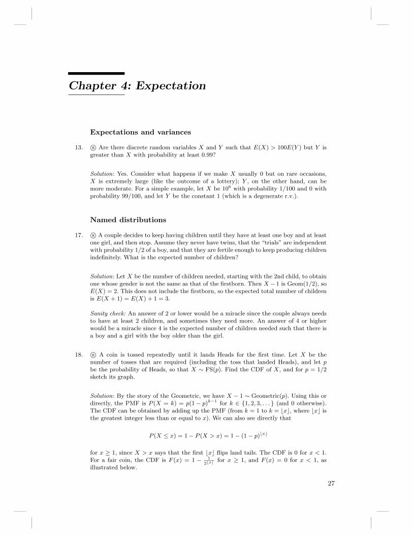
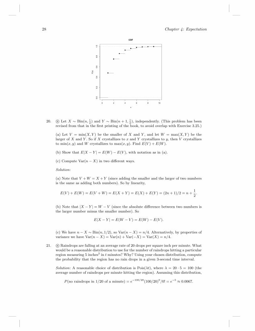
18. s© A coin is tossed repeatedly until it lands Heads for the first time. Let X be thenumber of tosses that are required (including the toss that landed Heads), and let pbe the probability of Heads, so that X ∼ FS(p). Find the CDF of X, and for p = 1/2sketch its graph.
Solution: By the story of the Geometric, we have X − 1 ∼ Geometric(p). Using this ordirectly, the PMF is P (X = k) = p(1− p)k−1 for k ∈ {1, 2, 3, . . . } (and 0 otherwise).The CDF can be obtained by adding up the PMF (from k = 1 to k = bxc, where bxc isthe greatest integer less than or equal to x). We can also see directly that
P (X ≤ x) = 1− P (X > x) = 1− (1− p)bxc
for x ≥ 1, since X > x says that the first bxc flips land tails. The CDF is 0 for x < 1.For a fair coin, the CDF is F (x) = 1 − 1
2bxcfor x ≥ 1, and F (x) = 0 for x < 1, as
illustrated below.
27
28 Chapter 4: Expectation
0 2 4 6 8 10
0.0
0.2
0.4
0.6
0.8
1.0
CDF
x
F(x)
20. s© Let X ∼ Bin(n, 12) and Y ∼ Bin(n + 1, 1
2), independently. (This problem has been
revised from that in the first printing of the book, to avoid overlap with Exercise 3.25.)
(a) Let V = min(X,Y ) be the smaller of X and Y , and let W = max(X,Y ) be thelarger of X and Y . So if X crystallizes to x and Y crystallizes to y, then V crystallizesto min(x, y) and W crystallizes to max(x, y). Find E(V ) + E(W ).
(b) Show that E|X − Y | = E(W )− E(V ), with notation as in (a).
(c) Compute Var(n−X) in two different ways.
Solution:
(a) Note that V +W = X + Y (since adding the smaller and the larger of two numbersis the same as adding both numbers). So by linearity,
E(V ) + E(W ) = E(V +W ) = E(X + Y ) = E(X) + E(Y ) = (2n+ 1)/2 = n+1
2.
(b) Note that |X − Y | = W − V (since the absolute difference between two numbers isthe larger number minus the smaller number). So
E|X − Y | = E(W − V ) = E(W )− E(V ).
(c) We have n−X ∼ Bin(n, 1/2), so Var(n−X) = n/4. Alternatively, by properties ofvariance we have Var(n−X) = Var(n) + Var(−X) = Var(X) = n/4.
21. s© Raindrops are falling at an average rate of 20 drops per square inch per minute. Whatwould be a reasonable distribution to use for the number of raindrops hitting a particularregion measuring 5 inches2 in t minutes? Why? Using your chosen distribution, computethe probability that the region has no rain drops in a given 3-second time interval.
Solution: A reasonable choice of distribution is Pois(λt), where λ = 20 · 5 = 100 (theaverage number of raindrops per minute hitting the region). Assuming this distribution,
P (no raindrops in 1/20 of a minute) = e−100/20(100/20)0/0! = e−5 ≈ 0.0067.

Chapter 4: Expectation 29
22. s© Alice and Bob have just met, and wonder whether they have a mutual friend. Eachhas 50 friends, out of 1000 other people who live in their town. They think that it’sunlikely that they have a friend in common, saying “each of us is only friends with 5%of the people here, so it would be very unlikely that our two 5%’s overlap.”
Assume that Alice’s 50 friends are a random sample of the 1000 people (equally likelyto be any 50 of the 1000), and similarly for Bob. Also assume that knowing who Alice’sfriends are gives no information about who Bob’s friends are.
(a) Compute the expected number of mutual friends Alice and Bob have.
(b) Let X be the number of mutual friends they have. Find the PMF of X.
(c) Is the distribution of X one of the important distributions we have looked at? If so,which?
Solution:
(a) Let Ij be the indicator r.v. for the jth person being a mutual friend. Then
E
(1000∑j=1
Ij
)= 1000E(I1) = 1000P (I1 = 1) = 1000 ·
(5
100
)2
= 2.5.
(b) Condition on who Alice’s friends are, and then count the number of ways that Bobcan be friends with exactly k of them. This gives
P (X = k) =
(50k
)(950
50−k
)(100050
)for 0 ≤ k ≤ 50 (and 0 otherwise).
(c) Yes, it is the Hypergeometric distribution, as shown by the PMF from (b) or bythinking of “tagging” Alice’s friends (like the elk) and then seeing how many taggedpeople there are among Bob’s friends.
24. s© Calvin and Hobbes play a match consisting of a series of games, where Calvin hasprobability p of winning each game (independently). They play with a “win by two”rule: the first player to win two games more than his opponent wins the match. Findthe expected number of games played.
Hint: Consider the first two games as a pair, then the next two as a pair, etc.
Solution: Think of the first 2 games, the 3rd and 4th, the 5th and 6th, etc. as “mini-matches.” The match ends right after the first mini-match which isn’t a tie. The proba-bility of a mini-match not being a tie is p2 + q2, so the number of mini-matches neededis 1 plus a Geom(p2 + q2) r.v. Thus, the expected number of games is 2
p2+q2.
Sanity check : For p = 0 or p = 1, this reduces to 2. The expected number of games ismaximized when p = 1
2, which makes sense intuitively. Also, it makes sense that the
result is symmetric in p and q.
26. s© Let X and Y be Pois(λ) r.v.s, and T = X + Y . Suppose that X and Y are notindependent, and in fact X = Y . Prove or disprove the claim that T ∼ Pois(2λ) in thisscenario.
Solution: The r.v. T = 2X is not Poisson: it can only take even values 0, 2, 4, 6, . . . ,whereas any Poisson r.v. has positive probability of being any of 0, 1, 2, 3, . . . .
Alternatively, we can compute the PMF of 2X, or note that Var(2X) = 4λ 6= 2λ =E(2X), whereas for any Poisson r.v. the variance equals the mean.
30 Chapter 4: Expectation
29. s© A discrete distribution has the memoryless property if for X a random variable withthat distribution, P (X ≥ j + k|X ≥ j) = P (X ≥ k) for all nonnegative integers j, k.
(a) If X has a memoryless distribution with CDF F and PMF pi = P (X = i), find anexpression for P (X ≥ j + k) in terms of F (j), F (k), pj , pk.
(b) Name a discrete distribution which has the memoryless property. Justify your answerwith a clear interpretation in words or with a computation.
Solution:
(a) By the memoryless property,
P (X ≥ k) = P (X ≥ j + k|X ≥ j) =P (X ≥ j + k,X ≥ j)
P (X ≥ j) =P (X ≥ j + k)
P (X ≥ j) ,
soP (X ≥ j + k) = P (X ≥ j)P (X ≥ k) = (1− F (j) + pj)(1− F (k) + pk).
(b) The Geometric distribution is memoryless (in fact, it turns out to be essentially theonly discrete memoryless distribution!). This follows from the story of the Geometric:consider Bernoulli trials, waiting for the first success (and defining waiting time to bethe number of failures before the first success). Say we have already had j failureswithout a success. Then the additional waiting time from that point forward has thesame distribution as the original waiting time (the Bernoulli trials neither are conspiringagainst the experimenter nor act as if he or she is due for a success: the trials areindependent). A calculation agrees: for X ∼ Geom(p),
P (X ≥ j + k|X ≥ j) =P (X ≥ j + k)
P (X ≥ j) =qj+k
qj= qk = P (X ≥ k).
Indicator r.v.s
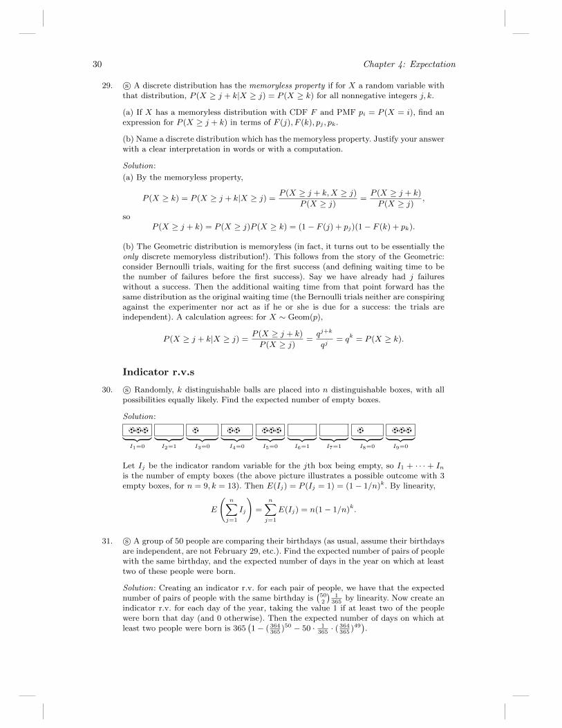
30. s© Randomly, k distinguishable balls are placed into n distinguishable boxes, with allpossibilities equally likely. Find the expected number of empty boxes.
Solution:
ooo︸ ︷︷ ︸I1=0
︸ ︷︷ ︸I2=1
o︸ ︷︷ ︸I3=0
oo︸ ︷︷ ︸I4=0
ooo︸ ︷︷ ︸I5=0
︸ ︷︷ ︸I6=1
︸ ︷︷ ︸I7=1
o︸ ︷︷ ︸I8=0
ooo︸ ︷︷ ︸I9=0
Let Ij be the indicator random variable for the jth box being empty, so I1 + · · · + Inis the number of empty boxes (the above picture illustrates a possible outcome with 3empty boxes, for n = 9, k = 13). Then E(Ij) = P (Ij = 1) = (1− 1/n)k. By linearity,
E
(n∑j=1
Ij
)=
n∑j=1
E(Ij) = n(1− 1/n)k.
31. s© A group of 50 people are comparing their birthdays (as usual, assume their birthdaysare independent, are not February 29, etc.). Find the expected number of pairs of peoplewith the same birthday, and the expected number of days in the year on which at leasttwo of these people were born.
Solution: Creating an indicator r.v. for each pair of people, we have that the expectednumber of pairs of people with the same birthday is
(502
)1
365by linearity. Now create an
indicator r.v. for each day of the year, taking the value 1 if at least two of the peoplewere born that day (and 0 otherwise). Then the expected number of days on which atleast two people were born is 365
(1− ( 364
365)50 − 50 · 1
365· ( 364
365)49).
Chapter 4: Expectation 31
32. s© A group of n ≥ 4 people are comparing their birthdays (as usual, assume theirbirthdays are independent, are not February 29, etc.). Let Iij be the indicator r.v. of iand j having the same birthday (for i < j). Is I12 independent of I34? Is I12 independentof I13? Are the Iij independent?
Solution: The indicator I12 is independent of the indicator I34 since knowing the birth-days of persons 1 and 2 gives us no information about the birthdays of persons 3 and4. Also, I12 is independent of I13 since even though both of these indicators involveperson 1, knowing that persons 1 and 2 have the same birthday gives us no informationabout whether persons 1 and 3 have the same birthday (this relies on the assumptionthat the 365 days are equally likely). In general, the indicator r.v.s here are pairwiseindependent. But they are not independent since, for example, if person 1 has the samebirthday as person 2 and person 1 has the same birthday as person 3, then persons 2and 3 must have the same birthday.
33. s© A total of 20 bags of Haribo gummi bears are randomly distributed to 20 students.Each bag is obtained by a random student, and the outcomes of who gets which bagare independent. Find the average number of bags of gummi bears that the first threestudents get in total, and find the average number of students who get at least one bag.
Solution: Let Xj be the number of bags of gummi bears that the jth student gets,and let Ij be the indicator of Xj ≥ 1. Then Xj ∼ Bin(20, 1
20), so E(Xj) = 1. So
E(X1 +X2 +X3) = 3 by linearity.
The average number of students who get at least one bag is
E(I1 + · · ·+ I20) = 20E(I1) = 20P (I1 = 1) = 20
(1−
(19
20
)20).
40. s© There are 100 shoelaces in a box. At each stage, you pick two random ends andtie them together. Either this results in a longer shoelace (if the two ends came fromdifferent pieces), or it results in a loop (if the two ends came from the same piece).What are the expected number of steps until everything is in loops, and the expectednumber of loops after everything is in loops? (This is a famous interview problem; leavethe latter answer as a sum.)
Hint: For each step, create an indicator r.v. for whether a loop was created then, andnote that the number of free ends goes down by 2 after each step.
Solution: Initially there are 200 free ends. The number of free ends decreases by 2 eachtime since either two separate pieces are tied together, or a new loop is formed. Soexactly 100 steps are always needed. Let Ij be the indicator r.v. for whether a new loopis formed at the jth step. At the time when there are n unlooped pieces (so 2n ends),the probability of forming a new loop is n
(2n2 )= 1
2n−1since any 2 ends are equally likely
to be chosen, and there are n ways to pick both ends of 1 of the n pieces. By linearity,the expected number of loops is
100∑n=1
1
2n− 1.
44. s© Let X be Hypergeometric with parameters w, b, n.
(a) Find E(X2
)by thinking, without any complicated calculations.
(b) Use (a) to find the variance of X. You should get
Var(X) =N − nN − 1
npq,
where N = w + b, p = w/N, q = 1− p.
32 Chapter 4: Expectation
Solution:
(a) In the story of the Hypergeometric,(X2
)is the number of pairs of draws such that
both balls are white. Creating an indicator r.v. for each pair, we have
E
(X
2
)=
(n
2
)w
w + b
w − 1
w + b− 1.
(b) By (a),
EX2 − EX = E(X(X − 1)) = n(n− 1)pw − 1
N − 1,
so
Var(X) = E(X2)− (EX)2
= n(n− 1)pw − 1
N − 1+ np− n2p2
= np
((n− 1)(w − 1)
N − 1+ 1− np
)= np
(nw − w − n+N
N − 1− nw
N
)= np
(Nnw −Nw −Nn+N2 −Nnw + nw
N(N − 1)
)= np
((N − n)(N − w)
N(N − 1)
)=N − nN − 1
npq.
47. s© A hash table is being used to store the phone numbers of k people, storing eachperson’s phone number in a uniformly random location, represented by an integer be-tween 1 and n (see Exercise 25 from Chapter 1 for a description of hash tables). Findthe expected number of locations with no phone numbers stored, the expected numberwith exactly one phone number, and the expected number with more than one phonenumber (should these quantities add up to n?).
Solution: Let Ij be an indicator random variable equal to 1 if the jth location is empty,and 0 otherwise, for 1 ≤ j ≤ n. Then P (Ij = 1) = (1− 1/n)k, since the phone numbersare stored in independent random locations. Then I1 + · · ·+ In is the number of emptylocations. By linearity of expectation, we have
E
(n∑j=1
Ij
)=
n∑j=1
E(Ij) = n(1− 1/n)k.
Similarly, the probability of a specific location having exactly 1 phone number stored iskn
(1 − 1n
)k−1, so the expected number of such locations is k(1 − 1/n)k−1. By linearity,the sum of the three expected values is n, so the expected number of locations withmore than one phone number is n− n(1− 1/n)k − k(1− 1/n)k−1.
50. s© Consider the following algorithm, known as bubble sort, for sorting a list of n distinctnumbers into increasing order. Initially they are in a random order, with all ordersequally likely. The algorithm compares the numbers in positions 1 and 2, and swapsthem if needed, then it compares the new numbers in positions 2 and 3, and swapsthem if needed, etc., until it has gone through the whole list. Call this one “sweep”through the list. After the first sweep, the largest number is at the end, so the secondsweep (if needed) only needs to work with the first n− 1 positions. Similarly, the thirdsweep (if needed) only needs to work with the first n − 2 positions, etc. Sweeps areperformed until n− 1 sweeps have been completed or there is a swapless sweep.
Chapter 4: Expectation 33
For example, if the initial list is 53241 (omitting commas), then the following 4 sweepsare performed to sort the list, with a total of 10 comparisons:
53241→ 35241→ 32541→ 32451→ 32415.
32415→ 23415→ 23415→ 23145.
23145→ 23145→ 21345.
21345→ 12345.
(a) An inversion is a pair of numbers that are out of order (e.g., 12345 has no inversions,while 53241 has 8 inversions). Find the expected number of inversions in the originallist.
(b) Show that the expected number of comparisons is between 12
(n2
)and
(n2
).
Hint: For one bound, think about how many comparisons are made if n− 1 sweeps aredone; for the other bound, use Part (a).
Solution:
(a) There are(n2
)pairs of numbers, each of which is equally likely to be in either order.
So by symmetry, linearity, and indicator r.v.s, the expected number of inversions is 12
(n2
).
(b) Let X be the number of comparisons and V be the number of inversions. On theone hand, X ≥ V since every inversion must be repaired. So E(X) ≥ E(V ) = 1
2
(n2
).
On the other hand, there are n− 1 comparisons needed in the first sweep, n− 2 in thesecond sweep (if needed), . . . , and 1 in the (n− 1)st sweep (if needed). So
X ≤ (n− 1) + (n− 2) + · · ·+ 2 + 1 =n(n− 1)
2=
(n
2
).
Hence, 12
(n2
)≤ E(X) ≤
(n2
).
52. s© An urn contains red, green, and blue balls. Balls are chosen randomly with replace-ment (each time, the color is noted and then the ball is put back). Let r, g, b be theprobabilities of drawing a red, green, blue ball, respectively (r + g + b = 1).
(a) Find the expected number of balls chosen before obtaining the first red ball, notincluding the red ball itself.
(b) Find the expected number of different colors of balls obtained before getting thefirst red ball.
(c) Find the probability that at least 2 of n balls drawn are red, given that at least 1 isred.
Solution:
(a) The distribution is Geom(r), so the expected value is 1−rr.
(b) Use indicator random variables: let I1 be 1 if green is obtained before red, and 0otherwise, and define I2 similarly for blue. Then
E(I1) = P (green before red) =g
g + r
since “green before red” means that the first nonblue ball is green. Similarly, E(I2) =b/(b+ r), so the expected number of colors obtained before getting red is
E(I1 + I2) =g
g + r+
b
b+ r.
(c) By definition of conditional probability,
P (at least 2 red| at least 1 red) =P (at least 2 red)
P (at least 1 red)=
1− (1− r)n − nr(1− r)n−1
1− (1− r)n .

34 Chapter 4: Expectation
53. s© Job candidates C1, C2, . . . are interviewed one by one, and the interviewer comparesthem and keeps an updated list of rankings (if n candidates have been interviewed sofar, this is a list of the n candidates, from best to worst). Assume that there is no limiton the number of candidates available, that for any n the candidates C1, C2, . . . , Cn areequally likely to arrive in any order, and that there are no ties in the rankings given bythe interview.
Let X be the index of the first candidate to come along who ranks as better than thevery first candidate C1 (so CX is better than C1, but the candidates after 1 but priorto X (if any) are worse than C1. For example, if C2 and C3 are worse than C1 but C4
is better than C1, then X = 4. All 4! orderings of the first 4 candidates are equallylikely, so it could have happened that the first candidate was the best out of the first 4candidates, in which case X > 4.
What is E(X) (which is a measure of how long, on average, the interviewer needs towait to find someone better than the very first candidate)?
Hint: Find P (X > n) by interpreting what X > n says about how C1 compares withother candidates, and then apply the result of Theorem 4.4.8.
Solution: For n ≥ 2, P (X > n) is the probability that none of C2, C3, . . . , Cn are bettercandidates than C1, i.e., the probability that the first candidate is the highest rankedout of the first n. Since any ordering of the first n candidates is equally likely, each of thefirst n is equally likely to be the highest ranked of the first n, so P (X > n) = 1/n. Forn = 0 or n = 1, P (X > n) = 1 (note that it does not make sense to say the probabilityis 1/n when n = 0). By Theorem 4.4.8,
E(X) =
∞∑n=0
P (X > n) = P (X > 0) +
∞∑n=1
P (X > n) = 1 +
∞∑n=1
1
n=∞
since the series is the harmonic series, which diverges.
How can the average waiting time to find someone better than the first candidate beinfinite? In the real world, there are always only finitely many candidates so the expectedwaiting time is finite, just as in the St. Petersburg paradox there must in reality be anupper bound on the number of rounds. The harmonic series diverges very slowly, soeven with millions of job candidates the average waiting time would not be very large.
LOTUS
56. s© For X ∼ Pois(λ), find E(X!) (the average factorial of X), if it is finite.
Solution: By LOTUS,
E(X!) = e−λ∞∑k=0
k!λk
k!=
e−λ
1− λ ,
for 0 < λ < 1 since this is a geometric series (and E(X!) is infinite if λ ≥ 1).
59. s© Let X ∼ Geom(p) and let t be a constant. Find E(etX), as a function of t (this isknown as the moment generating function; we will see in Chapter 6 how this functionis useful).
Solution: Letting q = 1− p, we have
E(etX) = p
∞∑k=0
etkqk = p
∞∑k=0
(qet)k =p
1− qet ,
for qet < 1 (while for qet ≥ 1, the series diverges).
Chapter 4: Expectation 35
60. s© The number of fish in a certain lake is a Pois(λ) random variable. Worried that theremight be no fish at all, a statistician adds one fish to the lake. Let Y be the resultingnumber of fish (so Y is 1 plus a Pois(λ) random variable).
(a) Find E(Y 2).
(b) Find E(1/Y ).
Solution:
(a) We have Y = X + 1 with X ∼ Pois(λ), so Y 2 = X2 + 2X + 1. So
E(Y 2) = E(X2 + 2X + 1) = E(X2) + 2E(X) + 1 = (λ+ λ2) + 2λ+ 1 = λ2 + 3λ+ 1,
since E(X2) = Var(X) + (EX)2 = λ+ λ2.
(b) By LOTUS,
E
(1
Y
)= E
(1
X + 1
)=
∞∑k=0
1
k + 1e−λ
λk
k!.
Using the identity k!(k + 1) = (k + 1)! and the Taylor series for eλ, this becomes
e−λ∞∑k=0
λk
(k + 1)!=e−λ
λ
∞∑k=0
λk+1
(k + 1)!=e−λ
λ(eλ − 1) =
1
λ(1− e−λ).
61. s© Let X be a Pois(λ) random variable, where λ is fixed but unknown. Let θ = e−3λ,and suppose that we are interested in estimating θ based on the data. Since X is whatwe observe, our estimator is a function of X, call it g(X). The bias of the estimator g(X)is defined to be E(g(X))− θ, i.e., how far off the estimate is on average; the estimatoris unbiased if its bias is 0.
(a) For estimating λ, the r.v. X itself is an unbiased estimator. Compute the bias of theestimator T = e−3X . Is it unbiased for estimating θ?
(b) Show that g(X) = (−2)X is an unbiased estimator for θ. (In fact, it turns out to bethe only unbiased estimator for θ.)
(c) Explain intuitively why g(X) is a silly choice for estimating θ, despite (b), and showhow to improve it by finding an estimator h(X) for θ that is always at least as good asg(X) and sometimes strictly better than g(X). That is,
|h(X)− θ| ≤ |g(X)− θ|,
with the inequality sometimes strict.
Solution:
(a) The estimator is biased, with bias given by
E(e−3X)− θ =∞∑k=0
e−3k λk
k!e−λ − e−3λ
= e−λ∞∑k=0
(e−3λ)k
k!− e−3λ
= e−λee−3λ − e−3λ
= e−3λ(e(2+e−3)λ − 1) 6= 0.
36 Chapter 4: Expectation
(b) The estimator g(X) = (−2)X is unbiased since
E(−2)X − θ =
∞∑k=0
(−2)kλk
k!e−λ − e−3λ
= e−λe−2λ − e−3λ = 0.
(c) The estimator g(X) is silly in the sense that it is sometimes negative, whereas e−3λ
is positive. One simple way to get a better estimator is to modify g(X) to make itnonnegative, by letting h(X) = 0 if g(X) < 0 and h(X) = g(X) otherwise.
Better yet, note that e−3λ is between 0 and 1 since λ > 0, so letting h(X) = 0 ifg(X) < 0 and h(X) = 1 if g(X) > 0 is clearly more sensible than using g(X).
Poisson approximation
62. s© Law school courses often have assigned seating to facilitate the Socratic method.Suppose that there are 100 first-year law students, and each takes the same two courses:Torts and Contracts. Both are held in the same lecture hall (which has 100 seats), andthe seating is uniformly random and independent for the two courses.
(a) Find the probability that no one has the same seat for both courses (exactly; youshould leave your answer as a sum).
(b) Find a simple but accurate approximation to the probability that no one has thesame seat for both courses.
(c) Find a simple but accurate approximation to the probability that at least two stu-dents have the same seat for both courses.
Solution:
(a) Let N be the number of students in the same seat for both classes. The problem hasessentially the same structure as the matching problem. Let Ej be the event that thejth student sits in the same seat in both classes. Then
P (N = 0) = 1− P
(100⋃j=1
Ej
).
By symmetry, inclusion-exclusion gives
P
(100⋃j=1
Ej
)=
100∑j=1
(−1)j−1
(100
j
)P
(j⋂
k=1
Ek
).
The j-fold intersection represents j particular students sitting pat throughout the twolectures, which occurs with probability (100− j)!/100!. So
P
(100⋃j=1
Ej
)=
100∑j=1
(−1)j−1
(100
j
)(100− j)!
100!=
100∑j=1
(−1)j−1/i!
P (N = 0) = 1−100∑j=1
(−1)j−1
j!=
100∑j=0
(−1)j
j!.
(b) Define Ii to be the indicator for student i having the same seat in both courses, sothat N =
∑100i=1 Ii. Then P (Ii = 1) = 1/100, and the Ii are weakly dependent because
P ((Ii = 1) ∩ (Ij = 1)) =
(1
100
)(1
99
)≈
(1
100
)2
= P (Ii = 1)P (Ij = 1).
Chapter 4: Expectation 37
So N is close to Pois(λ) in distribution, where λ = E(N) = 100E(I1) = 1. Thus,
P (N = 0) ≈ e−110/0! = e−1 ≈ 0.37.
This agrees with the result of (a), which we recognize as the Taylor series for ex, evalu-ated at x = −1.
(c) Using a Poisson approximation, we have
P (N ≥ 2) = 1− P (N = 0)− P (N = 1) ≈ 1− e−1 − e−1 = 1− 2e−1 ≈ 0.26.
63. s© A group of n people play “Secret Santa” as follows: each puts his or her name on aslip of paper in a hat, picks a name randomly from the hat (without replacement), andthen buys a gift for that person. Unfortunately, they overlook the possibility of drawingone’s own name, so some may have to buy gifts for themselves (on the bright side, somemay like self-selected gifts better). Assume n ≥ 2.
(a) Find the expected value of the number X of people who pick their own names.
(b) Find the expected number of pairs of people, A and B, such that A picks B’s nameand B picks A’s name (where A 6= B and order doesn’t matter).
(c) Let X be the number of people who pick their own names. What is the approximatedistribution of X if n is large (specify the parameter value or values)? What doesP (X = 0) converge to as n→∞?
Solution:
(a) Let Ij be the indicator r.v. for the jth person picking his or her own name. ThenE(Ij) = P (Ij = 1) = 1
n. By linearity, the expected number is n · E(Ij) = 1.
(b) Let Iij the the indicator r.v. for the ith and jth persons having such a swap (fori < j). Then E(Iij) = P (i picks j)P (j picks i|i picks j) = 1
n(n−1).
Alternatively, we can get this by counting: there are n! permutations for who pickswhom, of which (n − 2)! have i pick j and j pick i, giving (n−2)!
n!= 1
n(n−1). So by
linearity, the expected number is(n2
)· 1n(n−1)
= 12.
(c) By the Poisson paradigm, X is approximately Pois(1) for large n. As n → ∞,P (X = 0)→ 1/e, which is the probability of a Pois(1) r.v. being 0.
65. s© Ten million people enter a certain lottery. For each person, the chance of winning isone in ten million, independently.
(a) Find a simple, good approximation for the PMF of the number of people who winthe lottery.
(b) Congratulations! You won the lottery. However, there may be other winners. Assumenow that the number of winners other than you is W ∼ Pois(1), and that if there ismore than one winner, then the prize is awarded to one randomly chosen winner. Giventhis information, find the probability that you win the prize (simplify).
Solution:
(a) Let X be the number of people who win. Then
E(X) =107
107= 1.
A Poisson approximation is very good here since X is the number of “successes” for a

38 Chapter 4: Expectation
very large number of independent trials where the probability of success on each trial isvery low. So X is approximately Pois(1), and for k a nonnegative integer,
P (X = k) ≈ 1
e · k!.
(b) Let A be the event that you win the prize, and condition on W :
P (A) =
∞∑k=0
P (A|W = k)P (W = k) =1
e
∞∑k=0
1
k + 1
1
k!=
1
e
∞∑k=0
1
(k + 1)!=e− 1
e= 1− 1
e.
*Existence
68. s© Each of 111 people names his or her 5 favorite movies out of a list of 11 movies.
(a) Alice and Bob are 2 of the 111 people. Assume for this part only that Alice’s 5favorite movies out of the 11 are random, with all sets of 5 equally likely, and likewisefor Bob, independently. Find the expected number of movies in common to Alice’s andBob’s lists of favorite movies.
(b) Show that there are 2 movies such that at least 21 of the people name both of thesemovies as favorites.
Solution:
(a) Let Ij be the indicator for the jth movie being on both lists, for 1 ≤ j ≤ 11. Bysymmetry and linearity, the desired expected value is
11
(5
11
)2
=25
11.
(b) Choose 2 random movies (one at a time, without replacement). Let X be the numberof people who name both of these movies. Creating an indicator r.v. for each person,
E(X) = 111P (Alice names both random movies) = 111
(5
11· 4
10
)=
(111
110
)20 > 20,
since the first chosen movie has a 5/11 chance of being on Alice’s list and given that itis, the second chosen movie has a 4/10 chance of being on the list (or we can use theHypergeometric PMF after “tagging” Alice’s favorite movies).
Thus, there must exist 2 movies such that at least 21 of the people name both of themas favorites.
69. s© The circumference of a circle is colored with red and blue ink such that 2/3 of thecircumference is red and 1/3 is blue. Prove that no matter how complicated the coloringscheme is, there is a way to inscribe a square in the circle such that at least three of thefour corners of the square touch red ink.
Solution: Consider a random square, obtained by picking a uniformly random point onthe circumference and inscribing a square with that point a corner; say that the cornersare U1, . . . , U4, in clockwise order starting with the initial point chosen. Let Ij be theindicator r.v. of Uj touching red ink. By symmetry, E(Ij) = 2/3 so by linearity, theexpected number of corners touching red ink is 8/3. Thus, there must exist an inscribedsquare with at least 8/3 of its corners touching red ink. Such a square must have atleast 3 of its corners touching red ink.

Chapter 4: Expectation 39
70. s© A hundred students have taken an exam consisting of 8 problems, and for eachproblem at least 65 of the students got the right answer. Show that there exist twostudents who collectively got everything right, in the sense that for each problem, atleast one of the two got it right.
Solution: Say that the “score” of a pair of students is how many problems at least one ofthem got right. The expected score of a random pair of students (with all pairs equallylikely) is at least 8(1 − 0.352) = 7.02, as seen by creating an indicator r.v. for eachproblem for the event that at least one student in the pair got it right. (We can alsoimprove the 0.352 to 35
100· 3499
since the students are sampled without replacement.) Sosome pair of students must have gotten a score of at least 7.02, which means that theygot a score of at least 8.
71. s© Ten points in the plane are designated. You have ten circular coins (of the sameradius). Show that you can position the coins in the plane (without stacking them) sothat all ten points are covered.
Hint: Consider a honeycomb tiling of the plane (this is a way to divide the plane intohexagons). You can use the fact from geometry that if a circle is inscribed in a hexagonthen the ratio of the area of the circle to the area of the hexagon is π
2√3> 0.9.
Solution: Take a uniformly random honeycomb tiling (to do this, start with any honey-comb tiling and then shift it horizontally and vertically by uniformly random amounts;by periodicity there is an upper bound on how large the shifts need to be). Choosethe tiling so that a circle the same size as one of the coins can be inscribed in eachhexagon. Then inscribe a circle in each hexagon, and let Ij be the indicator r.v. for thejth point being contained inside one the circles. We have E(Ij) > 0.9 by the geometricfact mentioned above, so by linearity E(I1 + · · ·+ I10) > 9. Thus, there is a positioningof the honeycomb tiling such that all 10 points are contained inside the circles. Puttingcoins on top of the circles containing the points, we can cover all ten points.
72. s© Let S be a set of binary strings a1 . . . an of length n (where juxtaposition meansconcatenation). We call S k-complete if for any indices 1 ≤ i1 < · · · < ik ≤ n and anybinary string b1 . . . bk of length k, there is a string s1 . . . sn in S such that si1si2 . . . sik =b1b2 . . . bk. For example, for n = 3, the set S = {001, 010, 011, 100, 101, 110} is 2-completesince all 4 patterns of 0’s and 1’s of length 2 can be found in any 2 positions. Show thatif(nk
)2k(1− 2−k)m < 1, then there exists a k-complete set of size at most m.
Solution: Generate m random strings of length n independently, using fair coin flips todetermine each bit. Let S be the resulting random set of strings. If we can show thatthe probability that S is k-complete is positive, then we know that a k-complete set ofsize at most m must exist. Let A be the event that S is k-complete. Let N =
(nk
)2k
and let A1, . . . , AN be the events of the form “S contains a string which is b1 . . . bk atcoordinates i1 < · · · < ik,” in any fixed order. For example, if k = 3 then A1 could bethe event “S has an element which is 110 at positions 1, 2, 3.” Then P (A) > 0 since
P (Ac) = P (∪Nj=1Acj) ≤
N∑j=1
P (Acj) = N(1− 2−k)m < 1.
Mixed practice
75. s© A group of 360 people is going to be split into 120 teams of 3 (where the order ofteams and the order within a team don’t matter).
(a) How many ways are there to do this?
(b) The group consists of 180 married couples. A random split into teams of 3 is chosen,
40 Chapter 4: Expectation
with all possible splits equally likely. Find the expected number of teams containingmarried couples.
Solution:
(a) Imagine lining the people up and saying the first 3 are a team, the next 3 are ateam, etc. This overcounts by a factor of (3!)120 · 120! since the order within teams andthe order of teams don’t matter. So the number of ways is
360!
6120 · 120!.
(b) Let Ij be the indicator for the jth team having a married couple (taking the teamsto be chosen one at a time, or with respect to a random ordering). By symmetry andlinearity, the desired quantity is 120E(I1). We have
E(I1) = P (first team has a married couple) =180 · 358(
3603
) ,
since the first team is equally likely to be any 3 of the people, and to have a marriedcouple on the team we need to choose a couple and then any third person. So theexpected value is
120 · 180 · 358(3603
) .
(This simplifies to 120·180·358360·359·358/6 = 360
359. Another way to find the probability that the
first team has a married couple is to note that any particular pair in the team hasprobability 1
359of being married to each other, so since there are 3 disjoint possibilities
the probability is 3359
.)
76. s© The gambler de Mere asked Pascal whether it is more likely to get at least one six in4 rolls of a die, or to get at least one double-six in 24 rolls of a pair of dice. Continuingthis pattern, suppose that a group of n fair dice is rolled 4 · 6n−1 times.
(a) Find the expected number of times that “all sixes” is achieved (i.e., how often amongthe 4 · 6n−1 rolls it happens that all n dice land 6 simultaneously).
(b) Give a simple but accurate approximation of the probability of having at least oneoccurrence of “all sixes”, for n large (in terms of e but not n).
(c) de Mere finds it tedious to re-roll so many dice. So after one normal roll of the ndice, in going from one roll to the next, with probability 6/7 he leaves the dice in thesame configuration and with probability 1/7 he re-rolls. For example, if n = 3 and the7th roll is (3, 1, 4), then 6/7 of the time the 8th roll remains (3, 1, 4) and 1/7 of thetime the 8th roll is a new random outcome. Does the expected number of times that“all sixes” is achieved stay the same, increase, or decrease (compared with (a))? Give ashort but clear explanation.
Solution:
(a) Let Ij be the indicator r.v. for the event “all sixes” on the jth roll. Then E(Ij) =1/6n, so the expected value is 4 · 6n−1/6n = 2/3.
(b) By a Poisson approximation with λ = 2/3 (the expected value from (a)), the prob-ability is approximately 1− e−2/3.
(c) The answer stays the same, by the same reasoning as in (a), since linearity ofexpectation holds even for dependent r.v.s.
Chapter 4: Expectation 41
77. s© Five people have just won a $100 prize, and are deciding how to divide the $100 upbetween them. Assume that whole dollars are used, not cents. Also, for example, giving$50 to the first person and $10 to the second is different from vice versa.
(a) How many ways are there to divide up the $100, such that each gets at least $10?
(b) Assume that the $100 is randomly divided up, with all of the possible allocationscounted in (a) equally likely. Find the expected amount of money that the first personreceives.
(c) Let Aj be the event that the jth person receives more than the first person (for2 ≤ j ≤ 5), when the $100 is randomly allocated as in (b). Are A2 and A3 independent?
Solution:
(a) Give each person $10, and then distribute the remaining $50 arbitrarily. By Bose-Einstein (thinking of people as boxes and dollars as balls!), the number of ways is(
5 + 50− 1
50
)=
(54
50
)=
(54
4
).
(b) Let Xj be the amount that j gets. By symmetry, E(Xj) is the same for all j. ButX1 + · · ·+X5 = 100, so by linearity 100 = 5EX1. Thus, EX1 is $20.
(c) The events A2 and A3 are not independent since knowing that A2 occurred makes itmore likely that person 1 received a low percentage of the money, which in turn makesit more likely that A3 occurred.
78. s© Joe’s iPod has 500 different songs, consisting of 50 albums of 10 songs each. He listensto 11 random songs on his iPod, with all songs equally likely and chosen independently(so repetitions may occur).
(a) What is the PMF of how many of the 11 songs are from his favorite album?
(b) What is the probability that there are 2 (or more) songs from the same album amongthe 11 songs he listens to?
(c) A pair of songs is a match if they are from the same album. If, say, the 1st, 3rd, and7th songs are all from the same album, this counts as 3 matches. Among the 11 songshe listens to, how many matches are there on average?
Solution:
(a) The distribution is Bin(n, p) with n = 11, p = 150
(thinking of getting a song fromthe favorite album as a “success”). So the PMF is(
11
k
)(1
50
)k (49
50
)11−k
, for 0 ≤ k ≤ 11.
(b) This is a version of the birthday problem. We have
P (at least 1 match) = 1− P (no matches) = 1− 50 · 49 · · · · 40
5011= 1− 49!
39! · 5010.
(c) Defining an indicator r.v. Ijk for the event that the jth and kth songs match, wehave E(Ijk) = P (Ijk = 1) = 1/50, so the expected number of matches is(
11
2
)1
50=
11 · 10
2 · 50=
110
100= 1.1.
42 Chapter 4: Expectation
79. s© In each day that the Mass Cash lottery is run in Massachusetts, 5 of the integersfrom 1 to 35 are chosen (randomly and without replacement).
(a) When playing this lottery, find the probability of guessing exactly 3 numbers right,given that you guess at least 1 of the numbers right.
(b) Find an exact expression for the expected number of days needed so that all of the(355
)possible lottery outcomes will have occurred.
(c) Approximate the probability that after 50 days of the lottery, every number from 1to 35 has been picked at least once.
Solution:
(a) The distribution is Hypergeometric (think of capture-recapture, “tagging” the num-bers you choose). So
P (exactly 3 right|at least 1 right) =P (exactly 3 right)
1− P (none right)
=
(53
)(302
)/(355
)1−
(50
)(305
)/(355
) .(b) Let n =
(355
). By the coupon collector problem (or directly by linearity, writing the
expected number of days as a sum of Tj ’s with Tj − 1 a Geometric), the expected valueis
n
(1
n+
1
n− 1+ · · ·+ 1
2+ 1
).
(c) Let Aj be the event that j doesn’t get picked, so
P (Aj) = (30/35)50 = (6/7)50.
Let X be the number of Aj that occur. A Poisson approximation for X is reasonablesince these events are rare and weakly dependent. This gives
P (X = 0) ≈ e−35·(6/7)50 ≈ 0.98.

Chapter 5: Continuous random variables
Uniform and universality of the Uniform
11. s© Let U be a Uniform r.v. on the interval (−1, 1) (be careful about minus signs).
(a) Compute E(U),Var(U), and E(U4).
(b) Find the CDF and PDF of U2. Is the distribution of U2 Uniform on (0, 1)?
Solution:
(a) We have E(U) = 0 since the distribution is symmetric about 0. By LOTUS,
E(U2) =1
2
∫ 1
−1
u2du =1
3.
So Var(U) = E(U2)− (EU)2 = E(U2) = 13. Again by LOTUS,
E(U4) =1
2
∫ 1
−1
u4du =1
5.
(b) Let G(t) be the CDF of U2. Clearly G(t) = 0 for t ≤ 0 and G(t) = 1 for t ≥ 1,because 0 ≤ U2 ≤ 1. For 0 < t < 1,
G(t) = P (U2 ≤ t) = P (−√t ≤ U ≤
√t) =
√t,
since the probability of U being in an interval in (−1, 1) is proportional to its length.The PDF is G′(t) = 1
2t−1/2 for 0 < t < 1 (and 0 otherwise). The distribution of U2 is
not Uniform on (0, 1) as the PDF is not a constant on this interval (it is an example ofa Beta distribution, an important distribution that is introduced in Chapter 8).
12. s© A stick is broken into two pieces, at a uniformly random break point. Find the CDFand average of the length of the longer piece.
Solution: We can assume the units are chosen so that the stick has length 1. Let Lbe the length of the longer piece, and let the break point be U ∼ Unif(0, 1). For anyl ∈ [1/2, 1], observe that L < l is equivalent to {U < l and 1 − U < l}, which can bewritten as 1− l < U < l. We can thus obtain L’s CDF as
FL(l) = P (L < l) = P (1− l < U < l) = 2l − 1,
so L ∼ Unif(1/2, 1). In particular, E(L) = 3/4.
16. s© Let U ∼ Unif(0, 1), and
X = log
(U
1− U
).
Then X has the Logistic distribution, as defined in Example 5.1.6.
(a) Write down (but do not compute) an integral giving E(X2).
(b) Find E(X) without using calculus.
Hint: A useful symmetry property here is that 1− U has the same distribution as U .
43

44 Chapter 5: Continuous random variables
Solution:
(a) By LOTUS,
E(X2) =
∫ 1
0
(log
(u
1− u
))2
du.
(b) By the symmetry property mentioned in the hint, 1− U has the same distributionas U . So by linearity,
E(X) = E(logU − log(1− U)) = E(logU)− E(log(1− U)) = 0.
19. s© Let F be a CDF which is continuous and strictly increasing. Let µ be the mean ofthe distribution. The quantile function, F−1, has many applications in statistics andeconometrics. Show that the area under the curve of the quantile function from 0 to 1is µ.
Hint: Use LOTUS and universality of the Uniform.
Solution: We want to find∫ 1
0F−1(u)du. Let U ∼ Unif(0, 1) and X = F−1(U). By
universality of the Uniform, X ∼ F . By LOTUS,∫ 1
0
F−1(u)du = E(F−1(U)) = E(X) = µ.
Equivalently, make the substitution u = F (x), so du = f(x)dx, where f is the PDF ofthe distribution with CDF F . Then the integral becomes∫ ∞
−∞F−1(F (x))f(x)dx =
∫ ∞−∞
xf(x)dx = µ.
Sanity check : For the simple case that F is the Unif(0, 1) CDF, which is F (u) = u on(0, 1), we have
∫ 1
0F−1(u)du =
∫ 1
0udu = 1/2, which is the mean of a Unif(0, 1).
Normal
32. s© Let Z ∼ N (0, 1) and let S be a random sign independent of Z, i.e., S is 1 withprobability 1/2 and −1 with probability 1/2. Show that SZ ∼ N (0, 1).
Solution: Condition on S to find the CDF of SZ:
P (SZ ≤ x) = P (SZ ≤ x|S = 1)1
2+ P (SZ ≤ x|S = −1)
1
2
= P (Z ≤ x)1
2+ P (Z ≥ −x)
1
2
= P (Z ≤ x)1
2+ P (Z ≤ x)
1
2
= Φ(x),
where the penultimate equality is by symmetry of the Normal.
33. s© Let Z ∼ N (0, 1). Find E (Φ(Z)) without using LOTUS, where Φ is the CDF of Z.
Solution: By universality of the Uniform, F (X) ∼ Unif(0, 1) for any continuous randomvariable X with CDF F . Therefore, E(Φ(Z)) = 1/2.
Chapter 5: Continuous random variables 45
34. s© Let Z ∼ N (0, 1) and X = Z2. Then the distribution of X is called Chi-Square with1 degree of freedom. This distribution appears in many statistical methods.
(a) Find a good numerical approximation to P (1 ≤ X ≤ 4) using facts about the Normaldistribution, without querying a calculator/computer/table about values of the NormalCDF.
(b) Let Φ and ϕ be the CDF and PDF of Z, respectively. Show that for any t > 0,I(Z > t) ≤ (Z/t)I(Z > t). Using this and LOTUS, show that Φ(t) ≥ 1− ϕ(t)/t.
Solution:
(a) By symmetry of the Normal,
P (1 ≤ Z2 ≤ 4) = P (−2 ≤ Z ≤ −1 or 1 ≤ Z ≤ 2) = 2P (1 ≤ Z ≤ 2) = 2(Φ(2)− Φ(1)).
By the 68-95-99.7% Rule, P (−1 ≤ Z ≤ 1) ≈ 0.68. This says that 32% of the area underthe Normal curve is outside of [−1, 1], which by symmetry says that 16% is in (1,∞).So Φ(1) ≈ 1 − 0.16 = 0.84. Similarly, P (−2 ≤ Z ≤ 2) ≈ 0.95 gives Φ(2) ≈ 0.975. Ingeneral, symmetry of the Normal implies that for any t > 0,
P (−t ≤ Z ≤ t) = Φ(t)− Φ(−t) = 2Φ(t)− 1.
(b) The inequality I(Z > t) ≤ (Z/t)I(Z > t) is true since if the indicator is 0 then bothsides are 0, and if it is 1 then Z/t > 1. So
E(I(Z > t)) ≤ 1
tE(ZI(Z > t)) =
1
t
∫ ∞−∞
zI(z > t)ϕ(z)dz =1
t
∫ ∞t
zϕ(z)dz.
The integral can be done using a substitution: letting u = z2/2, we have∫ze−z
2/2dz =
∫e−udu = −e−u + C = −e−z
2/2 + C.
Thus,P (Z > t) = E(I(Z > t)) ≤ ϕ(t)/t,
which proves the desired bound on Φ(t).
36. s© Let Z ∼ N (0, 1). A measuring device is used to observe Z, but the device can onlyhandle positive values, and gives a reading of 0 if Z ≤ 0; this is an example of censoreddata. So assume that X = ZIZ>0 is observed rather than Z, where IZ>0 is the indicatorof Z > 0. Find E(X) and Var(X).
Solution: By LOTUS,
E(X) =1√2π
∫ ∞−∞
Iz>0ze−z2/2dz =
1√2π
∫ ∞0
ze−z2/2dz.
Letting u = z2/2, we have
E(X) =1√2π
∫ ∞0
e−udu =1√2π.
To obtain the variance, note that
E(X2) =1√2π
∫ ∞0
z2e−z2/2dz =
1
2
1√2π
∫ ∞−∞
z2e−z2/2dz =
1
2,
since a N (0, 1) r.v. has variance 1. Thus,
Var(X) = E(X2)− (EX)2 =1
2− 1
2π.
46 Chapter 5: Continuous random variables
Note that X is neither purely discrete nor purely continuous, since X = 0 with prob-ability 1/2 and P (X = x) = 0 for x 6= 0. So X has neither a PDF nor a PMF; butLOTUS still works, allowing us to work with the PDF of Z to study expected values offunctions of Z.
Sanity check : The variance is positive, as it should be. It also makes sense that thevariance is substantially less than 1 (which is the variance of Z), since we are reducingvariability by making the r.v. 0 half the time, and making it nonnegative rather thanroaming over the entire real line.
Exponential
38. s© A post office has 2 clerks. Alice enters the post office while 2 other customers, Boband Claire, are being served by the 2 clerks. She is next in line. Assume that the timea clerk spends serving a customer has the Exponential(λ) distribution.
(a) What is the probability that Alice is the last of the 3 customers to be done beingserved?
Hint: No integrals are needed.
(b) What is the expected total time that Alice needs to spend at the post office?
Solution:
(a) Alice begins to be served when either Bob or Claire leaves. By the memorylessproperty, the additional time needed to serve whichever of Bob or Claire is still there isExpo(λ). The time it takes to serve Alice is also Expo(λ), so by symmetry the probabilityis 1/2 that Alice is the last to be done being served.
(b) The expected time spent waiting in line is 12λ
, since the minimum of two independentExpo(λ) r.v.s is Expo(2λ) (by Example 5.6.3). The expected time spent being served is1λ
. So the expected total time is
1
2λ+
1
λ=
3
2λ.
41. s© Fred wants to sell his car, after moving back to Blissville (where he is happy withthe bus system). He decides to sell it to the first person to offer at least $15,000 forit. Assume that the offers are independent Exponential random variables with mean$10,000.
(a) Find the expected number of offers Fred will have.
(b) Find the expected amount of money that Fred will get for the car.
Solution:
(a) The offers on the car are i.i.d. Xi ∼ Expo(1/104). So the number of offers that aretoo low is Geom(p) with p = P (Xi ≥ 15000) = e−1.5. Including the successful offer, theexpected number of offers is thus (1− p)/p+ 1 = 1/p = e1.5.
(b) Let N be the number of offers, so the sale price of the car is XN . Note that
E(XN ) = E(X|X ≥ 12000)
for X ∼ Expo(1/104), since the successful offer is an Exponential for which our infor-mation is that the value is at least $15,000. To compute this, remember the memoryless
Chapter 5: Continuous random variables 47
property! For any a > 0, if X ∼ Expo(λ) then the distribution of X − a given X > a isitself Expo(λ). So
E(X|X ≥ 15000) = 15000 + E(X) = 25000,
which shows that Fred’s expected sale price is $25,000.
44. s© Joe is waiting in continuous time for a book called The Winds of Winter to bereleased. Suppose that the waiting time T until news of the book’s release is posted,measured in years relative to some starting point, has an Exponential distribution withλ = 1/5.
Joe is not so obsessive as to check multiple times a day; instead, he checks the websiteonce at the end of each day. Therefore, he observes the day on which the news wasposted, rather than the exact time T . Let X be this measurement, where X = 0 meansthat the news was posted within the first day (after the starting point), X = 1 meansit was posted on the second day, etc. (assume that there are 365 days in a year). Findthe PMF of X. Is this a named distribution that we have studied?
Solution: The event X = k is the same as the event k ≤ 365T < k+1, i.e., X = b365T c,where btc is the floor function of t (the greatest integer less than or equal to t). TheCDF of T is FT (t) = 1− e−t/5 for t > 0 (and 0 for t ≤ 0). So
P (X = k) = P
(k
365≤ T <
k + 1
365
)= FT
(k + 1
365
)−FT
(k
365
)= e−k/1825−e−(k+1)/1825.
This factors as(e−1/1825
)k(1− e−1/1825), which shows that X ∼ Geom(1− e−1/1825).
Sanity check : A Geometric distribution is plausible for a waiting time, and does takevalues 0, 1, 2, . . . . The parameter p = 1− e−1/1825 ≈ 0.0005 is very small, which reflectsboth the fact that there are a lot of days in a year (so each day is unlikely) and the factthat the author is not known for the celerity of his writing.
50. s© Find E(X3) for X ∼ Expo(λ), using LOTUS and the fact that E(X) = 1/λ andVar(X) = 1/λ2, and integration by parts at most once. In the next chapter, we’ll learnhow to find E(Xn) for all n.
Solution: By LOTUS,
E(X3) =
∫ ∞0
x3λe−λxdx = −x3e−λx∣∣∣∣∞0
+3
λ
∫ ∞0
x2λe−λxdx
=3
λE(X2) =
3
λ(V ar(X) + (EX)2) =
6
λ3,
where the second equality uses integration by parts, letting u = x3 and dv = λe−λxdxand we multiply the second term by 1 written as λ/λ.
51. s© The Gumbel distribution is the distribution of − logX with X ∼ Expo(1).
(a) Find the CDF of the Gumbel distribution.
(b) Let X1, X2, . . . be i.i.d. Expo(1) and let Mn = max(X1, . . . , Xn). Show that Mn −logn converges in distribution to the Gumbel distribution, i.e., as n → ∞ the CDF ofMn − logn converges to the Gumbel CDF.
Solution:
(a) Let G be Gumbel and X ∼ Expo(1). The CDF is
P (G ≤ t) = P (− logX ≤ t) = P (X ≥ e−t) = e−e−t
48 Chapter 5: Continuous random variables
for all real t.
(b) The CDF of Mn − logn is
P (Mn − logn ≤ t) = P (X1 ≤ t+ logn, . . . ,Xn ≤ t+ logn) = P (X1 ≤ t+ logn)n.
Using the Expo CDF and the fact that (1 + xn
)n → ex as n→∞, this becomes
(1− e−(t+logn))n = (1− e−t
n)n → e−e
−t.
Mixed practice
55. s© Consider an experiment where we observe the value of a random variable X, andestimate the value of an unknown constant θ using some random variable T = g(X) thatis a function of X. The r.v. T is called an estimator. Think of X as the data observedin the experiment, and θ as an unknown parameter related to the distribution of X.
For example, consider the experiment of flipping a coin n times, where the coin has anunknown probability θ of Heads. After the experiment is performed, we have observedthe value of X ∼ Bin(n, θ). The most natural estimator for θ is then X/n.
The bias of an estimator T for θ is defined as b(T ) = E(T )− θ. The mean squared erroris the average squared error when using T (X) to estimate θ:
MSE(T ) = E(T − θ)2.
Show thatMSE(T ) = Var(T ) + (b(T ))2 .
This implies that for fixed MSE, lower bias can only be attained at the cost of highervariance and vice versa; this is a form of the bias-variance tradeoff, a phenomenon whicharises throughout statistics.
Solution: Using the fact that adding a constant does not affect variance, we have
Var(T ) = Var(T − θ)
= E(T − θ)2 − (E(T − θ))2
= MSE(T )− (b(T ))2,
which proves the desired identity.
56. s© (a) Suppose that we have a list of the populations of every country in the world.
Guess, without looking at data yet, what percentage of the populations have the digit1 as their first digit (e.g., a country with a population of 1,234,567 has first digit 1 anda country with population 89,012,345 does not).
(b) After having done (a), look through a list of populations and count how many startwith a 1. What percentage of countries is this? Benford’s law states that in a very largevariety of real-life data sets, the first digit approximately follows a particular distributionwith about a 30% chance of a 1, an 18% chance of a 2, and in general
P (D = j) = log10
(j + 1
j
), for j ∈ {1, 2, 3, . . . , 9},
where D is the first digit of a randomly chosen element. (Exercise from Chapter 3 asksfor a proof that this is a valid PMF.) How closely does the percentage found in the dataagree with that predicted by Benford’s law?
Chapter 5: Continuous random variables 49
(c) Suppose that we write the random value in some problem (e.g., the population ofa random country) in scientific notation as X × 10N , where N is a nonnegative integerand 1 ≤ X < 10. Assume that X is a continuous r.v. with PDF
f(x) = c/x, for 1 ≤ x ≤ 10,
and 0 otherwise, with c a constant. What is the value of c (be careful with the basesof logs)? Intuitively, we might hope that the distribution of X does not depend on thechoice of units in which X is measured. To see whether this holds, let Y = aX witha > 0. What is the PDF of Y (specifying where it is nonzero)?
(d) Show that if we have a random number X×10N (written in scientific notation) andX has the PDF f from (c), then the first digit (which is also the first digit of X) hasBenford’s law as PMF.
Hint: What does D = j correspond to in terms of the values of X?
Solution:
(a) What did you guess?
(b) According to Wikipedia (as of October 15, 2011), 63 out of 225 countries have atotal population whose first digit is 1, which is 28%. (This depends slightly on whethercertain territories included in the Wikipedia list should be considered as “countries”but the purpose of this problem is not to delve into the sovereignty or nation-status ofterritories). It is striking that 28% of the countries have first digit 1, as this is so muchhigher than one would expect from guessing that the first digit is equally likely to beany of 1, 2, . . . , 9. This is an example of Benford’s law; similar phenomena have beenobserved in many different settings (such as with lengths of rivers, physical constants,and stock prices).
(c) The PDF (f(x) = c/x, 1 ≤ x ≤ 10) must integrate to one, by definition; therefore
1 = c
∫ 10
1
dx
x= c(ln 10− ln 1) = c ln 10.
So the constant of proportionality c = 1/ ln 10 = log10 e). If Y = aX (a change in scale),then Y has pdf c/y with the same value of c as before, except now a ≤ y ≤ 10a ratherthan 1 ≤ x ≤ 10. So the PDF takes the same form for aX as for X, but over a differentrange.
(d) The first digit D = d when d ≤ X < d+ 1. The probability of this is
P (D = d) = P (d ≤ X < d+ 1) =
∫ d+1
d
1
x ln 10dx,
which is log10(d+ 1)− log10(d), as desired.
57. s© (a) Let X1, X2, . . . be independent N (0, 4) r.v.s., and let J be the smallest value of jsuch that Xj > 4 (i.e., the index of the first Xj exceeding 4). In terms of Φ, find E(J).
(b) Let f and g be PDFs with f(x) > 0 and g(x) > 0 for all x. Let X be a randomvariable with PDF f . Find the expected value of the ratio
R =g(X)
f(X).
Such ratios come up very often in statistics, when working with a quantity knownas a likelihood ratio and when using a computational technique known as importancesampling.
50 Chapter 5: Continuous random variables
(c) Define
F (x) = e−e−x.
This is a CDF and is a continuous, strictly increasing function. Let X have CDF F , anddefine W = F (X). What are the mean and variance of W?
Solution:
(a) We have J − 1 ∼ Geom(p) with p = P (X1 > 4) = P (X1/2 > 2) = 1 − Φ(2), soE(J) = 1/(1− Φ(2)).
(b) By LOTUS,
Eg(X)
f(X)=
∫ ∞−∞
g(x)
f(x)f(x)dx =
∫ ∞−∞
g(x)dx = 1.
(c) By universality of the Uniform, W ∼ Unif(0, 1). Alternatively, we can computedirectly that the CDF of W is
P (W ≤ w) = P (F (X) ≤ w) = P (X ≤ F−1(w)) = F (F−1(w)) = w
for 0 < w < 1, so again we have W ∼ Unif(0, 1). Thus, E(W ) = 1/2 and Var(W ) = 1/12.
59. s© As in Example 5.7.3, athletes compete one at a time at the high jump. Let Xj behow high the jth jumper jumped, with X1, X2, . . . i.i.d. with a continuous distribution.We say that the jth jumper is “best in recent memory” if he or she jumps higher thanthe previous 2 jumpers (for j ≥ 3; the first 2 jumpers don’t qualify).
(a) Find the expected number of best in recent memory jumpers among the 3rd throughnth jumpers.
(b) Let Aj be the event that the jth jumper is the best in recent memory. Find P (A3 ∩A4), P (A3), and P (A4). Are A3 and A4 independent?
Solution:
(a) Let Ij be the indicator of the jth jumper being best in recent memory, for eachj ≥ 3. By symmetry, E(Ij) = 1/3 (similarly to examples from class and the homework).By linearity, the desired expected value is (n− 2)/3.
(b) The event A3 ∩ A4 occurs if and only if the ranks of the first 4 jumps are 4, 3, 2, 1or 3, 4, 2, 1 (where 1 denotes the best of the first 4 jumps, etc.). Since all orderings areequally likely,
P (A3 ∩A4) =2
4!=
1
12.
As in (a), we have P (A3) = P (A4) = 1/3. So P (A3 ∩A4) 6= P (A3)P (A4), which showsthat A3 and A4 are not independent.
Chapter 6: Moments
Moment generating functions
13. s© A fair die is rolled twice, with outcomes X for the first roll and Y for the secondroll. Find the moment generating function MX+Y (t) of X + Y (your answer should bea function of t and can contain unsimplified finite sums).
Solution: Since X and Y are i.i.d., LOTUS gives
MX+Y (t) = E(et(X+Y )) = E(etX)E(etY ) =
(1
6
6∑k=1
ekt)2
.
14. s© Let U1, U2, . . . , U60 be i.i.d. Unif(0, 1) and X = U1 + U2 + · · ·+ U60. Find the MGFof X.
Solution: The MGF of U1 is E(etU1) =∫ 1
0etudu = 1
t(et − 1) for t 6= 0 (and the value is
1 for t = 0). Thus, the MGF of X is
E(etX) = E(et(U1+···+U60)) =(E(etU1)
)60=
(et − 1)60
t60,
for t 6= 0 (and the value is 1 for t = 0).
20. s© Let X ∼ Pois(λ), and let M(t) be the MGF of X. The cumulant generating functionis defined to be g(t) = logM(t). Expanding g(t) as a Taylor series
g(t) =
∞∑j=1
cjj!tj
(the sum starts at j = 1 because g(0) = 0), the coefficient cj is called the jth cumulantof X. Find the jth cumulant of X, for all j ≥ 1.
Solution: Using the Taylor series for et,
g(t) = λ(et − 1) =
∞∑j=1
λtj
j!,
so cj = λ for all j ≥ 1.
21. s© Let Xn ∼ Bin(n, pn) for all n ≥ 1, where npn is a constant λ > 0 for all n (sopn = λ/n). Let X ∼ Pois(λ). Show that the MGF of Xn converges to the MGF of X(this gives another way to see that the Bin(n, p) distribution can be well-approximatedby the Pois(λ) when n is large, p is small, and λ = np is moderate).
Solution: Using the fact that (1 + x/n)n → ex as n→∞ (the compound interest limit,which is reviewed in the math appendix), we have
E(etXn) = (1− pn + pnet)n = (1 + λ(et − 1)/n)n → eλ(e
t−1) = E(etX).
51

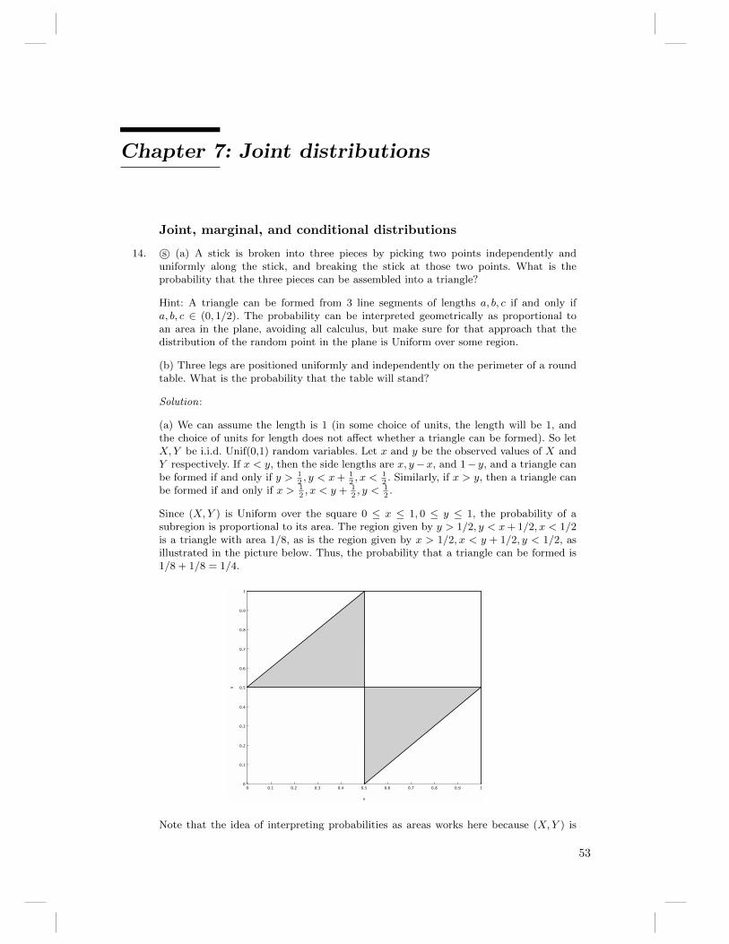
Chapter 7: Joint distributions
Joint, marginal, and conditional distributions
14. s© (a) A stick is broken into three pieces by picking two points independently anduniformly along the stick, and breaking the stick at those two points. What is theprobability that the three pieces can be assembled into a triangle?
Hint: A triangle can be formed from 3 line segments of lengths a, b, c if and only ifa, b, c ∈ (0, 1/2). The probability can be interpreted geometrically as proportional toan area in the plane, avoiding all calculus, but make sure for that approach that thedistribution of the random point in the plane is Uniform over some region.
(b) Three legs are positioned uniformly and independently on the perimeter of a roundtable. What is the probability that the table will stand?
Solution:
(a) We can assume the length is 1 (in some choice of units, the length will be 1, andthe choice of units for length does not affect whether a triangle can be formed). So letX,Y be i.i.d. Unif(0,1) random variables. Let x and y be the observed values of X andY respectively. If x < y, then the side lengths are x, y−x, and 1− y, and a triangle canbe formed if and only if y > 1
2, y < x+ 1
2, x < 1
2. Similarly, if x > y, then a triangle can
be formed if and only if x > 12, x < y + 1
2, y < 1
2.
Since (X,Y ) is Uniform over the square 0 ≤ x ≤ 1, 0 ≤ y ≤ 1, the probability of asubregion is proportional to its area. The region given by y > 1/2, y < x+ 1/2, x < 1/2is a triangle with area 1/8, as is the region given by x > 1/2, x < y + 1/2, y < 1/2, asillustrated in the picture below. Thus, the probability that a triangle can be formed is1/8 + 1/8 = 1/4.
10 0.1 0.2 0.3 0.4 0.5 0.6 0.7 0.8 0.9
1
0
0.1
0.2
0.3
0.4
0.5
0.6
0.7
0.8
0.9
x
y
Note that the idea of interpreting probabilities as areas works here because (X,Y ) is
53
54 Chapter 7: Joint distributions
Uniform on the square. For other distributions, in general we would need to find thejoint PDF of X,Y and integrate over the appropriate region.
(b) Think of the legs as points on a circle, chosen randomly one at a time, and chooseunits so that the circumference of the circle is 1. Let A,B,C be the arc lengths fromone point to the next (clockwise, starting with the first point chosen). Then
P (table falls) = P (the 3 legs are all contained in some semicircle)
= P (at least one of A,B,C is greater than 1/2) = 3/4,
by Part (a). So the probability that the table will stand is 1/4.
Alternatively, let Cj be the clockwise semicircle starting from the jth of the 3 points. LetAj be the event that Cj contains all 3 points. Then P (Aj) = 1/4 and with probability1, at most one Aj occurs. So P (A1 ∪ A2 ∪ A3) = 3/4, which again shows that theprobability that the table will stand is 1/4.
18. s© Let (X,Y ) be a uniformly random point in the triangle in the plane with vertices(0, 0), (0, 1), (1, 0). Find the joint PDF of X and Y , the marginal PDF of X, and theconditional PDF of X given Y .
Solution: The area of the triangle is 12, so the joint PDF of (X,Y ) is 2 inside the
triangle and 0 outside the triangle. The triangle is given by x ≥ 0, y ≥ 0, x + y ≤ 1,so the marginal PDF of X is
∫ 1−x0
2dy = 2(1 − x), for x ∈ [0, 1] (note that this isnonnegative and integrates to 1). The conditional PDF of X given Y is
fX|Y (x|y) =fX,Y (x, y)
fY (y)=
2
2(1− y)=
1
1− y ,
for (x, y) in the triangle (and 0 otherwise). Since 11−y is constant with respect to x, we
have X|Y ∼ Unif(0, 1− Y ).
19. s© A random point (X,Y, Z) is chosen uniformly in the ball B = {(x, y, z) : x2+y2+z2 ≤1}.
(a) Find the joint PDF of X,Y, Z.
(b) Find the joint PDF of X,Y .
(c) Find an expression for the marginal PDF of X, as an integral.
Solution:
(a) Just as in 2 dimensions uniform in a region means that probability is proportionalto area, in 3 dimensions probability is proportional to volume. That is,
P ((X,Y, Z) ∈ A) = c · volume(A)
if A is contained in B, where c is a constant. Letting A = B, we have that 1c
is 43π, the
volume of the ball. So the joint PDF of (X,Y, Z) is
f(x, y, z) =
{34π, if x2 + y2 + z2 ≤ 1;
0, otherwise.
(b) We just need to integrate out the z from the joint PDF of X,Y, Z. The limits ofintegration are found by noting that for any (x, y), we need to have z satisfy x2+y2+z2 ≤1.
fX,Y (x, y) =
∫ ∞−∞
f(x, y, z)dz
=3
4π
∫ √1−x2−y2
−√
1−x2−y2dz
=3
2π
√1− x2 − y2,
Chapter 7: Joint distributions 55
for x2 + y2 ≤ 1 (and the PDF is 0 otherwise).
(c) We can integrate out y, z from the joint PDF of X,Y, Z, or integrate out y from thejoint PDF of X,Y . Using the result of (b), we have for −1 ≤ x ≤ 1 that the marginalPDF of X is
fX(x) =3
2π
∫ √1−x2
−√
1−x2
√1− x2 − y2dy.
20. s© Let U1, U2, U3 be i.i.d. Unif(0, 1), and let L = min(U1, U2, U3),M = max(U1, U2, U3).
(a) Find the marginal CDF and marginal PDF of M, and the joint CDF and joint PDFof L,M .
Hint: For the latter, start by considering P (L ≥ l,M ≤ m).
(b) Find the conditional PDF of M given L.
Solution:
(a) The event M ≤ m is the same as the event that all 3 of the Uj are at most m, sothe CDF of M is FM (m) = m3 and the PDF is fM (m) = 3m2, for 0 ≤ m ≤ 1.
The event L ≥ l,M ≤ m is the same as the event that all 3 of the Uj are between l andm (inclusive), so
P (L ≥ l,M ≤ m) = (m− l)3
for m ≥ l with m, l ∈ [0, 1]. By the axioms of probability, we have
P (M ≤ m) = P (L ≤ l,M ≤ m) + P (L > l,M ≤ m).
So the joint CDF is
P (L ≤ l,M ≤ m) = m3 − (m− l)3,
for m ≥ l with m, l ∈ [0, 1]. The joint PDF is obtained by differentiating this withrespect to l and then with respect to m (or vice versa):
f(l,m) = 6(m− l),
for m ≥ l with m, l ∈ [0, 1]. As a check, note that getting the marginal PDF of M byfinding
∫m0f(l,m)dl does recover the PDF of M (the limits of integration are from 0 to
m since the min can’t be more than the max).
(b) The marginal PDF of L is fL(l) = 3(1− l)2 for 0 ≤ l ≤ 1 since P (L > l) = P (U1 >l, U2 > l, U3 > l) = (1−l)3 (alternatively, use the PDF of M together with the symmetrythat 1 − Uj has the same distribution as Uj , or integrate out m in the joint PDF ofL,M). So the conditional PDF of M given L is
fM|L(m|l) =f(l,m)
fL(l)=
2(m− l)(1− l)2 ,
for all m, l ∈ [0, 1] with m ≥ l.24. s© Two students, A and B, are working independently on homework (not necessarily for
the same class). Student A takes Y1 ∼ Expo(λ1) hours to finish his or her homework,while B takes Y2 ∼ Expo(λ2) hours.
(a) Find the CDF and PDF of Y1/Y2, the ratio of their problem-solving times.
(b) Find the probability that A finishes his or her homework before B does.
Solution:
56 Chapter 7: Joint distributions
(a) Let t > 0. The CDF of the ratio is
F (t) = P
(Y1
Y2≤ t)
= P (Y1 ≤ tY2)
=
∫ ∞0
(∫ ty2
0
λ1e−λ1y1dy1
)λ2e−λ2y2dy2
=
∫ ∞0
(1− e−λ1ty2)λ2e−λ2y2dy2
= 1−∫ ∞0
λ2e−(λ1t+λ2)y2dy2
= 1− λ2
tλ1 + λ2
=tλ1
tλ1 + λ2.
Of course, F (t) = 0 for t ≤ 0. The PDF of the ratio is
f(t) =d
dt
(tλ1
tλ1 + λ2
)=
λ1λ2
(λ1t+ λ2)2, for t > 0.
(b) Plugging in t = 1 above, we have
P (Y1 < Y2) =λ1
λ1 + λ2.
Alternatively, we can get the same result by applying Example 7.1.23. (The result canalso be derived without using calculus by thinking about Poisson processes, as shownin Chapter 13.)
26. s© The bus company from Blissville decides to start service in Blotchville, sensing apromising business opportunity. Meanwhile, Fred has moved back to Blotchville. Nowwhen Fred arrives at the bus stop, either of two independent bus lines may come by(both of which take him home). The Blissville company’s bus arrival times are exactly10 minutes apart, whereas the time from one Blotchville company bus to the next isExpo( 1
10). Fred arrives at a uniformly random time on a certain day.
(a) What is the probability that the Blotchville company bus arrives first?
Hint: One good way is to use the continuous law of total probability.
(b) What is the CDF of Fred’s waiting time for a bus?
Solution:
(a) Let U ∼ Unif(0, 10) be the arrival time of the next Blissville company bus, andX ∼ Expo( 1
10) be the arrival time of the next Blotchville company bus (the latter is
X ∼ Expo( 110
) by the memoryless property). Then
P (X < U) =
∫ 10
0
P (X < U |U = u)1
10du
=1
10
∫ 10
0
P (X < u|U = u)du
=1
10
∫ 10
0
(1− e−u/10)du =1
e.
(b) Let T = min(X,U) be the waiting time. Then
P (T > t) = P (X > t,U > t) = P (X > t)P (U > t).
Chapter 7: Joint distributions 57
So the CDF of T is
P (T ≤ t) = 1− P (X > t)P (U > t) = 1− e−t/10(1− t/10),
for 0 < t < 10 (and 0 for t ≤ 0, and 1 for t ≥ 10).
2D LOTUS
31. s© Let X and Y be i.i.d. Unif(0, 1). Find the standard deviation of the distance betweenX and Y .
Solution: Let W = |X − Y |. By 2-D LOTUS,
E(W ) =
∫ 1
0
∫ 1
0
|x− y|dxdy.
Split this into two parts (to get rid of the absolute values): x < y and x ≥ y (i.e., breakthe square into two triangles). By symmetry the integral over x < y equals the integralover x > y, so
E(W ) = 2
∫ 1
0
∫ y
0
(y − x)dxdy = 2
∫ 1
0
y2
2dy =
1
3.
Next, we find E(W 2). This can either be done by computing the double integral
E(W 2) =
∫ 1
0
∫ 1
0
(x− y)2dxdy,
or by writingE(W 2) = E(X − Y )2 = EX2 + EY 2 − 2E(XY ),
which is
2E(X2)− 2(EX)2 = 2Var(X) =1
6,
since E(XY ) = E(X)E(Y ) for X,Y independent, and E(X) = E(Y ) and E(X2) =E(Y 2) (as X and Y have the same distribution). Thus, E(W ) = 1/3,
Var(W ) = E(W 2)− (E(W ))2 =1
18,
and the standard deviation of the distance between X and Y is 1√18
= 1
3√2.
32. s© Let X,Y be i.i.d. Expo(λ). Find E|X−Y | in two different ways: (a) using 2D LOTUSand (b) using the memoryless property without any calculus.
Solution:
(a) First consider the case λ = 1. By LOTUS,
E|X − Y | =∫ ∞0
∫ ∞0
|x− y|e−xe−ydxdy
= 2
∫ ∞0
∫ ∞y
(x− y)e−xe−ydxdy
= 2
∫ ∞0
e−y∫ ∞y
(xe−x − ye−x)dxdy
= 2
∫ ∞0
e−y(−e−x(x+ 1) + ye−x
)|∞y dy
= 2
∫ ∞0
e−ye−ydy = 2
∫ ∞0
e−2ydy = 1.
For general λ, this and the fact that λX, λY are i.i.d. Expo(1) yield E|X − Y | = 1/λ.
(b) Write |X − Y | = max(X,Y ) − min(X,Y ). By the memoryless property, this isExpo(λ), as in Example 7.3.6. So E|X − Y | = 1
λ, which agrees with (a). (This also
shows Var(|X − Y |) = 1λ2 .)
58 Chapter 7: Joint distributions
Covariance
38. s© Let X and Y be r.v.s. Is it correct to say “max(X,Y ) + min(X,Y ) = X + Y ”? Is itcorrect to say “Cov(max(X,Y ),min(X,Y )) = Cov(X,Y ) since either the max is X andthe min is Y or vice versa, and covariance is symmetric”? Explain.
Solution: The identity max(x, y) + min(x, y) = x + y is true for all numbers x and y.The random variable M = max(X,Y ) is defined by M(s) = max(X(s), Y (s)); this justsays to perform the random experiment, observe the numerical values of X and Y , andtake their maximum. It follows that
max(X,Y ) + min(X,Y ) = X + Y
for all r.v.s X and Y , since whatever the outcome s of the random experiment is, wehave
max(X(s), Y (s)) + min(X(s), Y (s)) = X(s) + Y (s).
In contrast, the covariance of two r.v.s is a number, not a r.v.; it is not defined byobserving the values of the two r.v.s and then taking their covariance (that would bea useless quantity, since the covariance between two numbers is 0). It is wrong to say“Cov(max(X,Y ),min(X,Y )) = Cov(X,Y ) since either the max is X and the min isY or vice versa, and covariance is symmetric” since the r.v. X does not equal ther.v. max(X,Y ), nor does it equal the r.v. min(X,Y ).
To gain more intuition into this, consider a repeated sampling interpretation,where we independently repeat the same experiment many times and observe pairs(x1, y1), . . . , (xn, yn), where (xj , yj) is the observed value of (X,Y ) for the jthe exper-iment. Suppose that X and Y are independent non-constant r.v.s (and thus they areuncorrelated). Imagine a scatter plot of the observations (which is just a plot of thepoints (xj , yj)). Since X and Y are independent, there should be no trend in the plot.
On the other hand, imagine a scatter plot of the (max(xj , yj),min(xj , yj)) points. Herewe’d expect to see a clear increasing trend (since the max is always bigger than or equalto the min, so having a large value of the min (relative to its mean) should make itmore likely that we’ll have a large value of the max (relative to its mean). So it makessense that max(X,Y ) and min(X,Y ) should be positive correlated. This is illustratedin the plots below, in which we generated (X1, Y1), . . . , (X100, Y100) with the Xi’s andYj ’s i.i.d. N (0, 1).
−3 −2 −1 0 1 2 3
−3
−2
−1
01
23
x
y
−3 −2 −1 0 1 2 3
−3
−2
−1
01
23
max(x,y)
min
(x,y
)
The simulation was done in R, using the following code:
Chapter 7: Joint distributions 59
x <- rnorm(100); y <- rnorm(100)
plot(x,y, xlim=c(-3,3),ylim=c(-3,3), pch=16)
plot(pmax(x,y),pmin(x,y), xlim=c(-3,3),ylim=c(-3,3), xlab="max(x,y)",
ylab = "min(x,y)", pch=16)
39. s© Two fair six-sided dice are rolled (one green and one orange), with outcomes X andY respectively for the green and the orange.
(a) Compute the covariance of X + Y and X − Y .
(b) Are X + Y and X − Y independent?
Solution:
(a) We have
Cov(X + Y,X − Y ) = Cov(X,X)− Cov(X,Y ) + Cov(Y,X)− Cov(Y, Y ) = 0.
(b) They are not independent: information about X + Y may give information aboutX − Y , as shown by considering an extreme example. Note that if X + Y = 12, thenX = Y = 6, so X −Y = 0. Therefore, P (X −Y = 0|X +Y = 12) = 1 6= P (X −Y = 0),which shows that X+Y and X−Y are not independent. Alternatively, note that X+Yand X − Y are both even or both odd, since the sum (X + Y ) + (X − Y ) = 2X is even.
41. s© Let X and Y be standardized r.v.s (i.e., marginally they each have mean 0 andvariance 1) with correlation ρ ∈ (−1, 1). Find a, b, c, d (in terms of ρ) such that Z =aX + bY and W = cX + dY are uncorrelated but still standardized.
Solution: Let us look for a solution with Z = X, finding c and d to make Z and Wuncorrelated:
Cov(Z,W ) = Cov(X, cX + dY ) = Cov(X, cX) + Cov(X, dY ) = c+ dρ = 0.
Also, Var(W ) = c2 + d2 + 2cdρ = 1. Solving for c, d gives
a = 1, b = 0, c = −ρ/√
1− ρ2, d = 1/√
1− ρ2.
42. s© Let X be the number of distinct birthdays in a group of 110 people (i.e., the numberof days in a year such that at least one person in the group has that birthday). Underthe usual assumptions (no February 29, all the other 365 days of the year are equallylikely, and the day when one person is born is independent of the days when the otherpeople are born), find the mean and variance of X.
Solution: Let Ij be the indicator r.v. for the event that at least one of the peoplewas born on the jth day of the year, so X =
∑365j=1 Ij with Ij ∼ Bern(p), where p =
1− (364/365)110. The Ij ’s are dependent but by linearity, we still have
E(X) = 365p ≈ 95.083.
By symmetry, the variance is
Var(X) = 365Var(I1) + 2
(365
2
)Cov(I1, I2).
To get the covariance, note that Cov(I1, I2) = E(I1I2)−E(I1)E(I2) = E(I1I2)−p2, andE(I1I2) = P (I1I2 = 1) = P (A1 ∩ A2), where Aj is the event that at least one personwas born on the jth day of the year. The probability of the complement is
P (Ac1 ∪Ac2) = P (Ac1) + P (Ac2)− P (Ac1 ∩Ac2) = 2
(364
365
)110
−(
363
365
)110
,
so Var(X) = 365p(1− p) + 365 · 364 · (1− (2(364365
)110 − ( 363365
)110)− p2) ≈ 10.019.
60 Chapter 7: Joint distributions
47. s© Athletes compete one at a time at the high jump. Let Xj be how high the jthjumper jumped, with X1, X2, . . . i.i.d. with a continuous distribution. We say that thejth jumper sets a record if Xj is greater than all of Xj−1, . . . , X1.
Find the variance of the number of records among the first n jumpers (as a sum). Whathappens to the variance as n→∞?
Solution: Let Ij be the indicator r.v. for the jth jumper setting a record. By symmetry,E(Ij) = P (Ij = 1) = 1/j (as all of the first j jumps are equally likely to be the largestof those jumps). It was shown on Example 5.7.3 that I110 and I111 are independent.Similarly, Ii is independent of Ij for all i, j with i < j (in fact, they are independent,not just pairwise independent). To see this, note that by symmetry, learning that thejth jumper sets a record gives no information whatsoever about how the first i jumpersrank among themselves, or compute
P (Ii = Ij = 1) =
(j−1j−i−1
)(j − i− 1)!(i− 1)!
j!=
(i− 1)!(j − 1)!
i!j!=
1
ij= P (I1 = 1)P (I2 = 1),
where the numerator corresponds to putting the best of the first j jumps in position j,picking any j − 1 + 1 of the remaining jumps to fill positions i + 1 through j − 1 andputting them in any order, putting the best of the remaining i jumps in position i, andthen putting the remaining i− 1 jumps in any order.
The variance of Ij is Var(Ij) = E(I2j ) − (EIj)2 = 1
j− 1
j2. Since the Ij are pairwise
independent (and thus uncorrelated), the variance of I1 + · · ·+ In is
n∑j=1
(1
j− 1
j2
),
which goes to ∞ as n→∞ since∑nj=1
1j
diverges and∑nj=1
1j2
converges (to π2/6, as
it turns out).
48. s© A chicken lays a Pois(λ) number N of eggs. Each egg hatches a chick with probabilityp, independently. Let X be the number which hatch, so X|N = n ∼ Bin(n, p).
Find the correlation between N (the number of eggs) and X (the number of eggs whichhatch). Simplify; your final answer should work out to a simple function of p (the λshould cancel out).
Solution: By the chicken-egg story, X is independent of Y , with X ∼ Pois(λp) andY ∼ Pois(λq), for q = 1− p. So
Cov(N,X) = Cov(X + Y,X) = Cov(X,X) + Cov(Y,X) = Var(X) = λp,
giving
Corr(N,X) =λp
SD(N)SD(X)=
λp√λλp
=√p.
52. s© A drunken man wanders around randomly in a large space. At each step, he movesone unit of distance North, South, East, or West, with equal probabilities. Choosecoordinates such that his initial position is (0, 0) and if he is at (x, y) at some time, thenone step later he is at (x, y+ 1), (x, y− 1), (x+ 1, y), or (x− 1, y). Let (Xn, Yn) and Rnbe his position and distance from the origin after n steps, respectively.
General hint: Note that Xn is a sum of r.v.s with possible values −1, 0, 1, and likewisefor Yn, but be careful throughout the problem about independence.
(a) Determine whether or not Xn is independent of Yn.
(b) Find Cov(Xn, Yn).
Chapter 7: Joint distributions 61
(c) Find E(R2n).
Solution:
(a) They are not independent, as seen by considering an extreme case such as the eventthat the drunk headed East for the entire time: note that P (Yn = 0|Xn = n) = 1.
(b) WriteXn =∑ni=1 Zi and Yn =
∑nj=1Wj , where Zi is−1 if his ith step is Westward, 1
if his ith step is Eastward, and 0 otherwise, and similarly for Wj . Then Zi is independentof Wj for i 6= j. But Zi and Wi are highly dependent: exactly one of them is 0 sincehe moves in one direction at a time. Then Cov(Zi,Wi) = E(ZiWi) − E(Zi)E(Wi) = 0since ZiWi is always 0, and Zi and Wi have mean 0. So
Cov(Xn, Yn) =∑i,j
Cov(Zi,Wj) = 0.
(c) We have R2n = X2
n + Y 2n , and E(ZiZj) = 0 for i 6= j. So
E(R2n) = E(X2
n) + E(Y 2n ) = 2E(X2
n) = 2nE(Z21 ) = n,
since Z21 ∼ Bern(1/2).
53. s© A scientist makes two measurements, considered to be independent standard Normalr.v.s. Find the correlation between the larger and smaller of the values.
Hint: Note that max(x, y) + min(x, y) = x+ y and max(x, y)−min(x, y) = |x− y|.
Solution: Let X and Y be i.i.d N (0, 1) and M = max(X,Y ), L = min(X,Y ). By thehint,
E(M) + E(L) = E(M + L) = E(X + Y ) = E(X) + E(Y ) = 0,
E(M)− E(L) = E(M − L) = E|X − Y | = 2√π,
where the last equality was shown in Example 7.2.3. So E(M) = 1/√π, and
Cov(M,L) = E(ML)− E(M)E(L) = E(XY ) + (EM)2 = (EM)2 =1
π,
since ML = XY has mean E(XY ) = E(X)E(Y ) = 0. To obtain the correlation, wealso need Var(M) and Var(L). By symmetry of the Normal, (−X,−Y ) has the samedistribution as (X,Y ), so Var(M) = Var(L); call this v. Then
E(X − Y )2 = Var(X − Y ) = 2, and also
E(X − Y )2 = E(M − L)2 = EM2 + EL2 − 2E(ML) = 2v +2
π.
So v = 1 − 1π
(alternatively, we can get this by taking the variance of both sides ofmax(X,Y ) + min(X,Y ) = X + Y ). Thus,
Corr(M,L) =Cov(M,L)√
Var(M)Var(L)=
1/π
1− 1/π=
1
π − 1.
55. s© Consider the following method for creating a bivariate Poisson (a joint distributionfor two r.v.s such that both marginals are Poissons). Let X = V +W,Y = V +Z whereV,W,Z are i.i.d. Pois(λ) (the idea is to have something borrowed and something newbut not something old or something blue).
(a) Find Cov(X,Y ).
(b) Are X and Y independent? Are they conditionally independent given V ?
62 Chapter 7: Joint distributions
(c) Find the joint PMF of X,Y (as a sum).
Solution:
(a) Using the properties of covariance, we have
Cov(X,Y ) = Cov(V, V ) + Cov(V,Z) + Cov(W,V ) + Cov(W,Z) = Var(V ) = λ.
(b) Since X and Y are correlated (with covariance λ > 0), they are not independent.Alternatively, note that E(Y ) = 2λ but E(Y |X = 0) = λ since if X = 0 occurs thenV = 0 occurs. But X and Y are conditionally independent given V , since the conditionaljoint PMF is
P (X = x, Y = y|V = v) = P (W = x− v, Z = y − v|V = v)
= P (W = x− v, Z = y − v)
= P (W = x− v)P (Z = y − v)
= P (X = x|V = v)P (Y = y|V = v).
This makes sense intuitively since if we observe that V = v, then X and Y are theindependent r.v.s W and Z, shifted by the constant v.
(c) By (b), a good strategy is to condition on V :
P (X = x, Y = y) =
∞∑v=0
P (X = x, Y = y|V = v)P (V = v)
=
min(x,y)∑v=0
P (X = x|V = v)P (Y = y|V = v)P (V = v)
=
min(x,y)∑v=0
e−λλx−v
(x− v)!e−λ
λy−v
(y − v)!e−λ
λv
v!
= e−3λλx+ymin(x,y)∑v=0
λ−v
(x− v)!(y − v)!v!,
for x and y nonnegative integers. Note that we sum only up to min(x, y) since we knowfor sure that V ≤ X and V ≤ Y .
Sanity check : Note that P (X = 0, Y = 0) = P (V = 0,W = 0, Z = 0) = e−3λ.
Chicken-egg
59. s© A Pois(λ) number of people vote in a certain election. Each voter votes for candidateA with probability p and for candidate B with probability q = 1− p, independently ofall the other voters. Let V be the difference in votes, defined as the number of votes forA minus the number for B.
(a) Find E(V ).
(b) Find Var(V ).
Solution:
(a) Let X and Y be the number of votes for A and B respectively, and let N = X + Y .Then X|N ∼ Bin(N, p) and Y |N ∼ Bin(N, q). By Adam’s Law or the chicken-egg story,E(X) = λp and E(Y ) = λq. So
E(V ) = E(X − Y ) = E(X)− E(Y ) = λ(p− q).
(b) By the chicken-egg story, X ∼ Pois(λp) and Y ∼ Pois(λq) are independent. So
Var(X − Y ) = Var(X) + Var(Y ) = λp+ λq = λ.
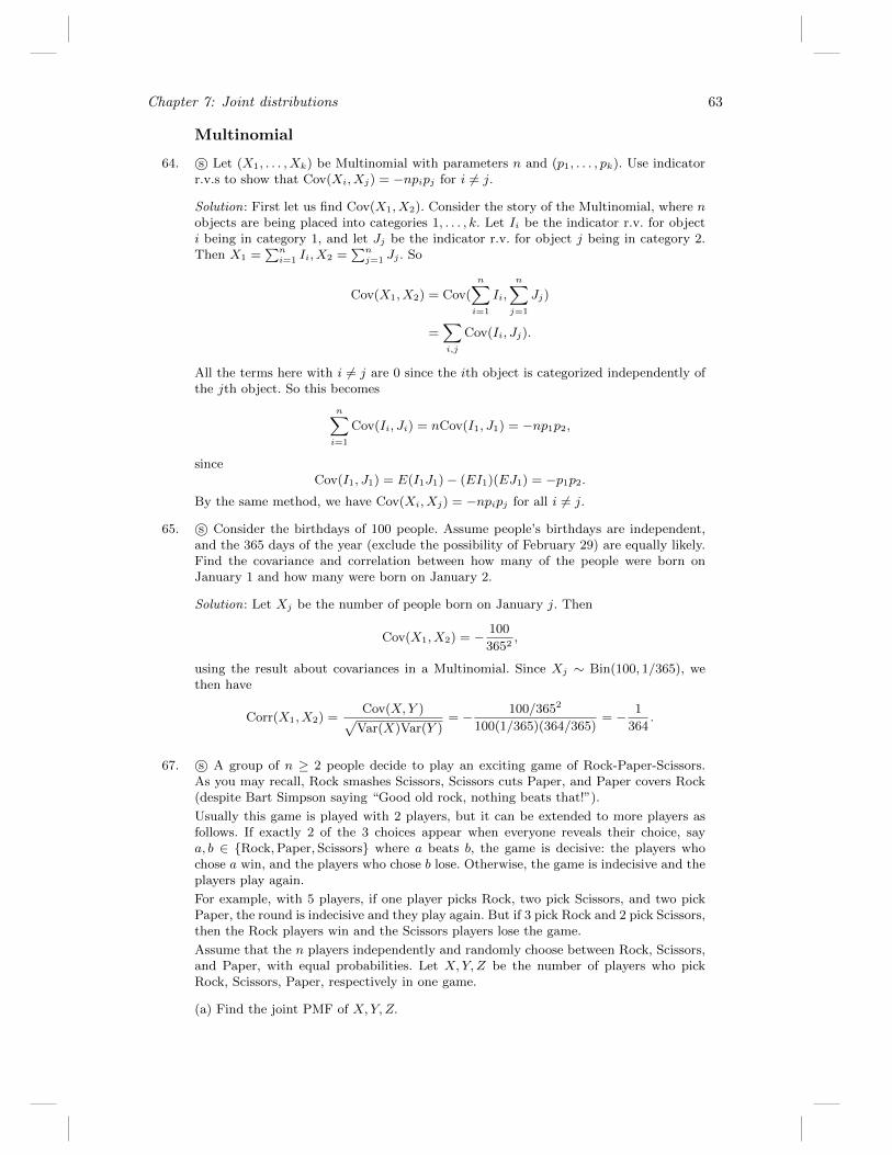
Chapter 7: Joint distributions 63
Multinomial
64. s© Let (X1, . . . , Xk) be Multinomial with parameters n and (p1, . . . , pk). Use indicatorr.v.s to show that Cov(Xi, Xj) = −npipj for i 6= j.
Solution: First let us find Cov(X1, X2). Consider the story of the Multinomial, where nobjects are being placed into categories 1, . . . , k. Let Ii be the indicator r.v. for objecti being in category 1, and let Jj be the indicator r.v. for object j being in category 2.Then X1 =
∑ni=1 Ii, X2 =
∑nj=1 Jj . So
Cov(X1, X2) = Cov(
n∑i=1
Ii,
n∑j=1
Jj)
=∑i,j
Cov(Ii, Jj).
All the terms here with i 6= j are 0 since the ith object is categorized independently ofthe jth object. So this becomes
n∑i=1
Cov(Ii, Ji) = nCov(I1, J1) = −np1p2,
sinceCov(I1, J1) = E(I1J1)− (EI1)(EJ1) = −p1p2.
By the same method, we have Cov(Xi, Xj) = −npipj for all i 6= j.
65. s© Consider the birthdays of 100 people. Assume people’s birthdays are independent,and the 365 days of the year (exclude the possibility of February 29) are equally likely.Find the covariance and correlation between how many of the people were born onJanuary 1 and how many were born on January 2.
Solution: Let Xj be the number of people born on January j. Then
Cov(X1, X2) = − 100
3652,
using the result about covariances in a Multinomial. Since Xj ∼ Bin(100, 1/365), wethen have
Corr(X1, X2) =Cov(X,Y )√
Var(X)Var(Y )= − 100/3652
100(1/365)(364/365)= − 1
364.
67. s© A group of n ≥ 2 people decide to play an exciting game of Rock-Paper-Scissors.As you may recall, Rock smashes Scissors, Scissors cuts Paper, and Paper covers Rock(despite Bart Simpson saying “Good old rock, nothing beats that!”).
Usually this game is played with 2 players, but it can be extended to more players asfollows. If exactly 2 of the 3 choices appear when everyone reveals their choice, saya, b ∈ {Rock,Paper, Scissors} where a beats b, the game is decisive: the players whochose a win, and the players who chose b lose. Otherwise, the game is indecisive and theplayers play again.
For example, with 5 players, if one player picks Rock, two pick Scissors, and two pickPaper, the round is indecisive and they play again. But if 3 pick Rock and 2 pick Scissors,then the Rock players win and the Scissors players lose the game.
Assume that the n players independently and randomly choose between Rock, Scissors,and Paper, with equal probabilities. Let X,Y, Z be the number of players who pickRock, Scissors, Paper, respectively in one game.
(a) Find the joint PMF of X,Y, Z.
64 Chapter 7: Joint distributions
(b) Find the probability that the game is decisive. Simplify your answer.
(c) What is the probability that the game is decisive for n = 5? What is the limitingprobability that a game is decisive as n→∞? Explain briefly why your answer makessense.
Solution:
(a) The joint PMF of X,Y, Z is
P (X = a, Y = b, Z = c) =n!
a!b!c!
(1
3
)a+b+cwhere a, b, c are any nonnegative integers with a + b + c = n, since (1/3)a+b+c is theprobability of any specific configuration of choices for each player with the right numbersin each category, and the coefficient in front counts the number of distinct ways topermute such a configuration.
Alternatively, we can write the joint PMF as
P (X = a, Y = b, Z = c) = P (X = a)P (Y = b|X = a)P (Z = c|X = a, Y = b),
where for a + b + c = n, P (X = a) can be found from the Bin(n, 1/3) PMF, P (Y =b|X = a) can be found from the Bin(n− a, 1/2) PMF, and P (Z = c|X = a, Y = b) = 1.
This is a Mult3(n, ( 13, 13, 13)) distribution.
(b) The game is decisive if and only if exactly one of X,Y, Z is 0. These cases are disjointso by symmetry, the probability is 3 times the probability that X is zero and Y and Zare nonzero. Note that if X = 0 and Y = k, then Z = n− k. This gives
P (decisive) = 3
n−1∑k=1
n!
0!k!(n− k)!
(1
3
)n
= 3
(1
3
)n n−1∑k=1
(n
k
)
=2n − 2
3n−1
since∑n−1k=1
(nk
)= −1 − 1 +
∑nk=0
(nk
)= 2n − 2 (by the binomial theorem or the fact
that a set with n elements has 2n subsets). As a check, when n = 2 this reduces to 2/3,which makes sense since for 2 players, the game is decisive if and only if the two playersdo not pick the same choice.
(c) For n = 5, the probability is (25−2)/34 = 30/81 ≈ 0.37. As n→∞, (2n−2)/3n−1 →0, which make sense since if the number of players is very large, it is very likely thatthere will be at least one of each of Rock, Paper, and Scissors.
68. s© Emails arrive in an inbox according to a Poisson process with rate λ (so the numberof emails in a time interval of length t is distributed as Pois(λt), and the numbers ofemails arriving in disjoint time intervals are independent). Let X,Y, Z be the numbers ofemails that arrive from 9 am to noon, noon to 6 pm, and 6 pm to midnight (respectively)on a certain day.
(a) Find the joint PMF of X,Y, Z.
(b) Find the conditional joint PMF of X,Y, Z given that X + Y + Z = 36.
(c) Find the conditional PMF of X+Y given that X+Y +Z = 36, and find E(X+Y |X+Y +Z = 36) and Var(X +Y |X +Y +Z = 36) (conditional expectation and conditional
Chapter 7: Joint distributions 65
variance given an event are defined in the same way as expectation and variance, usingthe conditional distribution given the event in place of the unconditional distribution).
Solution:
(a) Since X ∼ Pois(3λ), Y ∼ Pois(6λ), Z ∼ Pois(6λ) independently, the joint PMF is
P (X = x, Y = y, Z = z) =e−3λ(3λ)x
x!
e−6λ(6λ)y
y!
e−6λ(6λ)z
z!,
for any nonnegative integers x, y, z.
(b) Let T = X+Y +Z ∼ Pois(15λ), and suppose that we observe T = t. The conditionalPMF is 0 for x+ y + z 6= t. For x+ y + z = t,
P (X = x, Y = y, Z = z|T = t) =P (T = t|X = x, Y = y, Z = z)P (X = x, Y = y, Z = z)
P (T = t)
=
e−3λ(3λ)x
x!e−6λ(6λ)y
ye−6λ(6λ)z
z!
e−15λ(15λ)t
t!
=t!
x!y!z!
(3
15
)x(6
15
)y (6
15
)z.
Thus, (X,Y, Z) is conditionally Multinomial given T = t, and we have that (X,Y, Z) isconditionally Mult3(36, ( 1
5, 25, 25)) given T = 36.
(c) Let W = X + Y and T = X + Y + Z. Using the story of the Multinomial and Part(b), we can merge the categories “9 am to noon” and “noon to 6 pm” to get
W |T = 36 ∼ Bin
(36,
9
15
).
Therefore, E(W |T = 36) = 36 · 915
= 21.6 and Var(W |T = 36) = 36 · 915· 615
= 8.64.
Multivariate Normal
71. s© Let (X,Y ) be Bivariate Normal, with X and Y marginally N (0, 1) and with corre-lation ρ between X and Y .
(a) Show that (X + Y,X − Y ) is also Bivariate Normal.
(b) Find the joint PDF of X + Y and X − Y (without using calculus), assuming −1 <ρ < 1.
Solution:
(a) The linear combination s(X + Y ) + t(X − Y ) = (s+ t)X + (s− t)Y is also a linearcombination of X and Y , so it is Normal, which shows that (X + Y,X − Y ) is MVN.
(b) Since X+Y and X−Y are uncorrelated (as Cov(X+Y,X−Y ) = Var(X)−Var(Y ) =0) and (X+Y,X−Y ) is MVN, they are independent. Marginally, X+Y ∼ N (0, 2+2ρ)and X − Y ∼ N (0, 2− 2ρ). Thus, the joint PDF is
f(s, t) =1
4π√
1− ρ2e−
14(s2/(1+ρ)+t2/(1−ρ)).
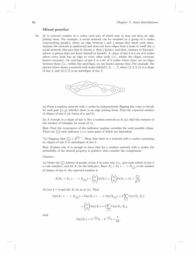
66 Chapter 7: Joint distributions
Mixed practice
84. s© A network consists of n nodes, each pair of which may or may not have an edgejoining them. For example, a social network can be modeled as a group of n nodes(representing people), where an edge between i and j means they know each other.Assume the network is undirected and does not have edges from a node to itself (for asocial network, this says that if i knows j, then j knows i and that, contrary to Socrates’advice, a person does not know himself or herself). A clique of size k is a set of k nodeswhere every node has an edge to every other node (i.e., within the clique, everyoneknows everyone). An anticlique of size k is a set of k nodes where there are no edgesbetween them (i.e., within the anticlique, no one knows anyone else). For example, thepicture below shows a network with nodes labeled 1, 2, . . . , 7, where {1, 2, 3, 4} is a cliqueof size 4, and {3, 5, 7} is an anticlique of size 3.
12
3
7
4
5 6
(a) Form a random network with n nodes by independently flipping fair coins to decidefor each pair {x, y} whether there is an edge joining them. Find the expected numberof cliques of size k (in terms of n and k).
(b) A triangle is a clique of size 3. For a random network as in (a), find the variance ofthe number of triangles (in terms of n).
Hint: Find the covariances of the indicator random variables for each possible clique.There are
(n3
)such indicator r.v.s, some pairs of which are dependent.
*(c) Suppose that(nk
)< 2(k2)−1. Show that there is a network with n nodes containing
no cliques of size k or anticliques of size k.
Hint: Explain why it is enough to show that for a random network with n nodes, theprobability of the desired property is positive; then consider the complement.
Solution:
(a) Order the(nk
)subsets of people of size k in some way (i.e., give each subset of size k
a code number), and let Xi be the indicator. Since X1 +X2 + · · ·+X(nk)is the number
of cliques of size k, the expected number is
E(X1 +X2 + · · ·+X(nk)) =
(n
k
)E(X1) =
(n
k
)P (X1 = 1) =
(nk
)2(k2)
.
(b) Let k = 3 and the Xi be as in (a). Then
Var(X1 + · · ·+X(n3)) = Var(X1) + · · ·+ Var(X(n3)) + 2∑i<j
Cov(Xi, Xj)
=
(n
3
)Var(X1) + 2
∑i<j
Cov(Xi, Xj),
with
Var(X1) = 2−(32)(1− 2−(32)) =7
64.
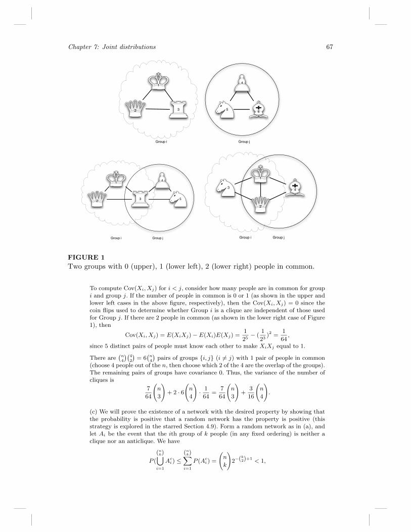
Chapter 7: Joint distributions 67
Group i Group j
3
4
6 5
1
2
3
4
5
1
2
Group i Group j
3
2
1
4
Group i Group j
FIGURE 1
Two groups with 0 (upper), 1 (lower left), 2 (lower right) people in common.
To compute Cov(Xi, Xj) for i < j, consider how many people are in common for groupi and group j. If the number of people in common is 0 or 1 (as shown in the upper andlower left cases in the above figure, respectively), then the Cov(Xi, Xj) = 0 since thecoin flips used to determine whether Group i is a clique are independent of those usedfor Group j. If there are 2 people in common (as shown in the lower right case of Figure1), then
Cov(Xi, Xj) = E(XiXj)− E(Xi)E(Xj) =1
25− (
1
23)2 =
1
64,
since 5 distinct pairs of people must know each other to make XiXj equal to 1.
There are(n4
)(42
)= 6(n4
)pairs of groups {i, j} (i 6= j) with 1 pair of people in common
(choose 4 people out of the n, then choose which 2 of the 4 are the overlap of the groups).The remaining pairs of groups have covariance 0. Thus, the variance of the number ofcliques is
7
64
(n
3
)+ 2 · 6
(n
4
)· 1
64=
7
64
(n
3
)+
3
16
(n
4
).
(c) We will prove the existence of a network with the desired property by showing thatthe probability is positive that a random network has the property is positive (thisstrategy is explored in the starred Section 4.9). Form a random network as in (a), andlet Ai be the event that the ith group of k people (in any fixed ordering) is neither aclique nor an anticlique. We have
P (
(nk)⋃i=1
Aci ) ≤(nk)∑i=1
P (Aci ) =
(n
k
)2−(k2)+1 < 1,
68 Chapter 7: Joint distributions
which shows that
P (
(nk)⋂i=1
Ai) = 1− P (
(nk)⋃i=1
Aci ) > 0,
as desired. Alternatively, let C be the number of cliques of size k and A be the numberof anticliques of size k, and write C +A = T . Then
E(T ) = E(C) + E(A) =
(n
k
)2−(k2)+1 < 1,
by the method of Part (a). So P (T = 0) > 0, since P (T ≥ 1) = 1 would imply E(T ) ≥ 1.This again shows that there must be a network with the desired property.
85. s© Shakespeare wrote a total of 884647 words in his known works. Of course, manywords are used more than once, and the number of distinct words in Shakespeare’sknown writings is 31534 (according to one computation). This puts a lower bound onthe size of Shakespeare’s vocabulary, but it is likely that Shakespeare knew words whichhe did not use in these known writings.
More specifically, suppose that a new poem of Shakespeare were uncovered, and considerthe following (seemingly impossible) problem: give a good prediction of the number ofwords in the new poem that do not appear anywhere in Shakespeare’s previously knownworks.
Ronald Thisted and Bradley Efron studied this problem in the papers [9] and [10],developing theory and methods and then applying the methods to try to determinewhether Shakespeare was the author of a poem discovered by a Shakespearean scholarin 1985. A simplified version of their method is developed in the problem below. Themethod was originally invented by Alan Turing (the founder of computer science) andI.J. Good as part of the effort to break the German Enigma code during World War II.
Let N be the number of distinct words that Shakespeare knew, and assume these wordsare numbered from 1 to N . Suppose for simplicity that Shakespeare wrote only twoplays, A and B. The plays are reasonably long and they are of the same length. Let Xjbe the number of times that word j appears in play A, and Yj be the number of timesit appears in play B, for 1 ≤ j ≤ N .
(a) Explain why it is reasonable to model Xj as being Poisson, and Yj as being Poissonwith the same parameter as Xj .
(b) Let the numbers of occurrences of the word “eyeball” (which was coined by Shake-speare) in the two plays be independent Pois(λ) r.v.s. Show that the probability that“eyeball” is used in play B but not in play A is
e−λ(λ− λ2/2! + λ3/3!− λ4/4! + . . . ).
(c) Now assume that λ from (b) is unknown and is itself taken to be a random variableto reflect this uncertainty. So let λ have a PDF f0. Let X be the number of times theword “eyeball” appears in play A and Y be the corresponding value for play B. Assumethat the conditional distribution of X,Y given λ is that they are independent Pois(λ)r.v.s. Show that the probability that “eyeball” is used in play B but not in play A isthe alternating series
P (X = 1)− P (X = 2) + P (X = 3)− P (X = 4) + . . . .
Hint: Condition on λ and use (b).
(d) Assume that every word’s numbers of occurrences in A and B are distributed as in
Chapter 7: Joint distributions 69
(c), where λ may be different for different words but f0 is fixed. Let Wj be the number ofwords that appear exactly j times in play A. Show that the expected number of distinctwords appearing in play B but not in play A is
E(W1)− E(W2) + E(W3)− E(W4) + . . . .
(This shows that W1 −W2 +W3 −W4 + . . . is an unbiased predictor of the number ofdistinct words appearing in play B but not in play A: on average it is correct. Moreover,it can be computed just from having seen play A, without needing to know f0 or any ofthe λj . This method can be extended in various ways to give predictions for unobservedplays based on observed plays.)
Solution:
(a) It is reasonable to model Xj and Yj as Poisson, because this distribution is used todescribe the number of “events” (such as emails received) happening at some averagerate in a fixed interval or volume. The Poisson paradigm applies here: each individualword in a play has some very small probability of being word j, and the words areweakly dependent. Here an event means using word j, the average rate is determined byhow frequently Shakespeare uses that word overall. It is reasonable to assume that theaverage rate of occurrence of a particular word is the same for two plays by the sameauthor, so we take λ to be the same for Xj and Yj .
(b) Let X be the number of times that “eyeball” is used in play A, and Y be the numberof times that it is used in play B. Since X and Y are independent Pois(λ),
P (X = 0, Y > 0) = P (X = 0) (1− P (Y = 0)) = e−λ(
1− e−λ)
= e−λ(
1−(
1− λ+λ2
2!− λ3
3!+λ4
4!− . . .
))= e−λ
(λ− λ2
2!+λ3
3!− λ4
4!+ . . .
).
(c) Now λ is a random variable. Given λ, the calculation from (b) holds. By the law oftotal probability,
P (X = 0, Y > 0) =
∫ ∞0
P (X = 0, Y > 0 | λ)f0(λ)dλ
=
∫ ∞0
P (X = 1 | λ)f0(λ)dλ−∫ ∞0
P (X = 2 | λ)f0(λ)dλ
+
∫ ∞0
P (X = 3 | λ)f0(λ)dλ−∫ ∞0
P (X = 4 | λ)f0(λ)dλ+ . . .
= P (X = 1)− P (X = 2) + P (X = 3)− P (X = 4) + . . .
(d) Let Xj be the number of times word j appears in play A and let W be the numberof distinct words that appear in play B but not in A. Then W =
∑Nj=1 Ij , where Ij is
the indicator r.v. of the event that word j appears in play B but not in play A, and Nis the total number of words. By (c), for 1 ≤ j ≤ N ,
EIj =
∞∑i=1
(−1)i+1P (Xj = i).
Also, note that the number of words that appear exactly i times in play A is
Wi = I(X1 = i) + I(X2 = i) + I(X3 = i) + · · ·+ I(XN = i),
70 Chapter 7: Joint distributions
where I(Xj = i) is the indicator of word j appearing exactly i times in play A. So
EWi =
N∑j=1
EI(Xj = i) =
N∑j=1
P (Xj = i).
Then
EW =
N∑j=1
EIj =
N∑j=1
∞∑i=1
(−1)i+1P (Xj = i)
=
∞∑i=1
(−1)i+1N∑j=1
P (Xj = i)
=
∞∑i=1
(−1)i+1EWi
= EW1 − EW2 + EW3 − EW4 + . . . .
Chapter 8: Transformations
Change of variables
4. s© Find the PDF of Z4 for Z ∼ N (0, 1).
Solution: Let Y = Z4. For y > 0, the CDF of Y is
P (Y ≤ y) = P (Z4 ≤ y) = P (−y1/4 ≤ Z ≤ y1/4) = Φ(y1/4)− Φ(−y1/4) = 2Φ(y1/4)− 1.
So the PDF is
fY (y) =2
4y−3/4ϕ(y1/4) =
1
2√
2πy−3/4e−y
1/2/2,
for y > 0, where ϕ is the N (0, 1) PDF.
6. s© Let U ∼ Unif(0, 1). Find the PDFs of U2 and√U .
Solution:
(PDF of U2.) Let Y = U2, 0 < u < 1, and y = u2, so u =√y. The absolute Jacobian
determinant is∣∣∣ dudy ∣∣∣ =
∣∣∣ 12√y
∣∣∣ = 12√y
for 0 < y < 1. The PDF of Y for 0 < y < 1 is
fY (y) = fU (u)
∣∣∣∣dudy∣∣∣∣ =
1
2√y,
with fY (y) = 0 otherwise. This is the Beta( 12, 1) PDF, so Y = U2 ∼ Beta( 1
2, 1).
(PDF of√U .) Now let Y = U1/2, 0 < u < 1, and y = u1/2, so u = y2. The absolute
Jacobian determinant is∣∣∣ dudy ∣∣∣ = |2y| = 2y for 0 < y < 1. The PDF of Y for 0 < y < 1 is
fY (y) = fU (u)
∣∣∣∣dudy∣∣∣∣ = 2y,
with fY (y) = 0 otherwise. This says that Y has a Beta(2,1) distribution.
In general, the same method shows that U1α ∼ Beta(α, 1) for any α > 0.
16. s© Let X,Y be continuous r.v.s with a spherically symmetric joint distribution, whichmeans that the joint PDF is of the form f(x, y) = g(x2 + y2) for some function g. Let(R, θ) be the polar coordinates of (X,Y ), so R2 = X2 +Y 2 is the squared distance fromthe origin and θ is the angle (in [0, 2π)), with X = R cos θ, Y = R sin θ.
(a) Explain intuitively why R and θ are independent. Then prove this by finding thejoint PDF of (R, θ).
(b) What is the joint PDF of (R, θ) when (X,Y ) is Uniform in the unit disk {(x, y) :x2 + y2 ≤ 1}?
(c) What is the joint PDF of (R, θ) when X and Y are i.i.d. N (0, 1)?
Solution:
(a) Intuitively, this makes sense since the joint PDF of X,Y at a point (x, y) only
71
72 Chapter 8: Transformations
depends on the distance from (x, y) to the origin, not on the angle, so knowing R givesno information about θ. The absolute Jacobian is r (as shown on the math reviewhandout), so
fR,θ(r, t) = fX,Y (x, y)r = r · g(r2)
for all r ≥ 0, t ∈ [0, 2π). This factors as a function of r times a (constant) function of t,so R and θ are independent with θ ∼ Unif(0, 2π).
(b) We have fX,Y (x, y) = 1π
for x2 + y2 ≤ 1, so fR,θ(r, t) = rπ
for 0 ≤ r ≤ 1, t ∈ [0, 2π)(and the PDF is 0 otherwise). This says that R and θ are independent with marginalPDFs fR(r) = 2r for 0 ≤ r ≤ 1 and fθ(t) = 1
2πfor 0 ≤ t < 2π.
(c) The joint PDF of X,Y is 12πe−(x2+y2)/2, so g(r2) = 1
2πe−r
2/2 and the joint PDF
of (R, θ) is 12πre−r
2/2. This says that R and θ are independent with marginal PDFs
fR(r) = re−r2/2 for r ≥ 0 and fθ(t) = 1
2πfor 0 ≤ t < 2π. (The distribution of R is an
example of a Weibull ; note that it is the distribution of W 1/2 for W ∼ Expo(1/2).)
Convolutions
24. s© Let X and Y be independent positive r.v.s, with PDFs fX and fY respectively, andconsider the product T = XY . When asked to find the PDF of T , Jacobno arguesthat “it’s like a convolution, with a product instead of a sum. To have T = t we needX = x and Y = t/x for some x; that has probability fX(x)fY (t/x), so summing upthese possibilities we get that the PDF of T is
∫∞0fX(x)fY (t/x)dx.” Evaluate Jacobno’s
argument, while getting the PDF of T (as an integral) in 2 ways:
(a) using the continuous version of the law of total probability to get the CDF, andthen taking the derivative (you can assume that swapping the derivative and integral isvalid);
(b) by taking the log of both sides of T = XY and doing a convolution (and thenconverting back to get the PDF of T ).
Solution:
(a) By the law of total probability (conditioning on X),
P (T ≤ t) =
∫ ∞0
P (XY ≤ t|X = x)fX(x)dx
=
∫ ∞0
P (Y ≤ t/x|X = x)fX(x)dx
=
∫ ∞0
FY (t/x)fX(x)dx,
which has derivative
fT (t) =
∫ ∞0
fX(x)fY (t/x)dx
x.
This is not the same as Jacobno claimed: there is an extra x in the denominator. Thisstems from the fact that the transformation (X,Y ) to (XY,X) is nonlinear, in contrastto the transformation (X,Y ) to (X+Y,X) considered in SP 8 # 2.3. Jacobno is ignoringthe distinction between probabilities and probability densities, and is implicitly (andincorrectly) assuming that there is no Jacobian term.
(b) Let Z = log(T ),W = log(X), V = log(Y ), so Z = W + V . The PDF of Z is
fZ(z) =
∫ ∞−∞
fW (w)fV (z − w)dw,
Chapter 8: Transformations 73
where by change of variables fW (w) = fX(ew)ew, fV (v) = fY (ev)ev. So
fZ(z) =
∫ ∞−∞
fX(ew)ewfY (ez−w)ez−wdw = ez∫ ∞−∞
fX(ew)fY (ez−w)dw.
Transforming back to T , we have
fT (t) = fZ(log t)1
t=
∫ ∞−∞
fX(ew)fY (elog(t)−w)dw =
∫ ∞0
fX(x)fY (t/x)dx
x,
letting x = ew. This concurs with (a): Jacobno is missing the x in the denominator.
Beta and Gamma
29. s© Let B ∼ Beta(a, b). Find the distribution of 1−B in two ways: (a) using a change ofvariables and (b) using a story proof. Also explain why the result makes sense in termsof Beta being the conjugate prior for the Binomial.
Solution:
(a) Let W = 1 − B. The function g(t) = 1 − t is strictly decreasing with absolutederivative | − 1| = 1, so the PDF of W is
fW (w) =Γ(a+ b)
Γ(a)Γ(b)(1− w)a−1wb−1,
for 0 < w < 1, which shows that W ∼ Beta(b, a).
(b) Using the bank–post office story, we can represent B = XX+Y
with X ∼ Gamma(a, 1)
and Y ∼ Gamma(b, 1) independent. Then 1−B = YX+Y
∼ Beta(b, a) by the same story.
This result makes sense intuitively since if we use Beta(a, b) as the prior distributionfor the probability p of success in a Binomial problem, interpreting a as the number ofprior successes and b as the number of prior failures, then 1 − p is the probability offailure and, interchanging the roles of “success” and “failure,” it makes sense to have1− p ∼ Beta(b, a).
30. s© Let X ∼ Gamma(a, λ) and Y ∼ Gamma(b, λ) be independent, with a and b integers.Show that X +Y ∼ Gamma(a+ b, λ) in three ways: (a) with a convolution integral; (b)with MGFs; (c) with a story proof.
Solution:
(a) The convolution integral is
fX+Y (t) =
∫ ∞−∞
fX(x)fY (t−x)dx =
∫ t
0
1
Γ(a)
1
Γ(b)(λx)a(λ(t−x))be−λxe−λ(t−x)
1
x
1
t− xdx,
where we integrate from 0 to t since we need x > 0 and t− x > 0. This is
λa+be−λt
Γ(a)Γ(b)
∫ t
0
xa−1(t−x)b−1dx = λa+be−λt
Γ(a)Γ(b)
Γ(a)Γ(b)
Γ(a+ b)ta+b−1 =
1
Γ(a+ b)(λt)a+be−λt
1
t,
using a Beta integral (after letting u = x/t so that we can integrate from 0 to 1 ratherthan 0 to t). Thus, X + Y ∼ Gamma(a+ b, λ).
(b) The MGF of X + Y is MX(t)MY (t) = λa
(λ−t)aλb
(λ−t)b = λa+b
(λ−t)a+b = MX+Y (t), which
again shows that X + Y ∼ Gamma(a+ b, λ).
(c) Interpret X as the time of the ath arrival in a Poisson process with rate λ, and Yas the time needed for b more arrivals to occur (which is independent of X since thetimes between arrivals are independent Expo(λ) r.v.s). Then X + Y is the time of the(a+ b)th arrival, so X + Y ∼ Gamma(a+ b, λ).
74 Chapter 8: Transformations
32. s© Fred waits X ∼ Gamma(a, λ) minutes for the bus to work, and then waits Y ∼Gamma(b, λ) for the bus going home, with X and Y independent. Is the ratio X/Yindependent of the total wait time X + Y ?
Solution: As shown in the bank–post office story, W = XX+Y
is independent of X + Y .So any function of W is independent of any function of X + Y . And we have that X/Yis a function of W , since
X
Y=
XX+Y
YX+Y
=W
1−W ,
so X/Y is independent of X + Y .
33. s© The F -test is a very widely used statistical test based on the F (m,n) distribution,
which is the distribution of X/mY/n
with X ∼ Gamma(m2, 12), Y ∼ Gamma(n
2, 12). Find the
distribution of mV/(n+mV ) for V ∼ F (m,n).
Solution: Let X ∼ Gamma(m2, 12), Y ∼ Gamma(n
2, 12), and V = n
mXY
. Then
mV/(n+mV ) =nX/Y
n+ nX/Y=
X
X + Y∼ Beta
(m2,n
2
).
34. s© Customers arrive at the Leftorium store according to a Poisson process with rate λcustomers per hour. The true value of λ is unknown, so we treat it as a random variable.Suppose that our prior beliefs about λ can be expressed as λ ∼ Expo(3). Let X be thenumber of customers who arrive at the Leftorium between 1 pm and 3 pm tomorrow.Given that X = 2 is observed, find the posterior PDF of λ.
Solution: It follows from Story 8.4.5 (Gamma-Poisson conjugacy) that the posteriordistribution of λ given the data is Gamma(3, 5). Equivalently, we can use Bayes’ ruledirectly. Writing f0 for the prior PDF and f1 for the posterior PDF, we have
f1(λ|x) =P (X = x|λ)f0(λ)
P (X = x),
where f0(λ) = 3e−3λ for λ > 0, and P (X = x|λ) is obtained from the Pois(2λ) PMF.For x = 2, the numerator is
e−2λ(2λ)2
2!· 3e−3λ = 6λ2e−5λ.
The denominator does not depend on λ, so it serves as a normalizing constant forthe posterior PDF. So the posterior PDF is proportional to λ2e−5λ, which shows thatthe posterior distribution is Gamma(3, 5). Including the normalizing constant for theGamma distribution, we have
f1(λ|2) =53
Γ(3)λ2e−5λ =
125
2λ2e−5λ,
for λ > 0.
35. s© Let X and Y be independent, positive r.v.s. with finite expected values.
(a) Give an example where E( XX+Y
) 6= E(X)E(X+Y )
, computing both sides exactly.
Hint: Start by thinking about the simplest examples you can think of!
(b) If X and Y are i.i.d., then is it necessarily true that E( XX+Y
) = E(X)E(X+Y )
?
(c) Now let X ∼ Gamma(a, λ) and Y ∼ Gamma(b, λ). Show without using calculus that
E
(Xc
(X + Y )c
)=
E(Xc)
E((X + Y )c)
Chapter 8: Transformations 75
for every real c > 0.
Solution:
(a) As a simple example, let X take on the values 1 and 3 with probability 1/2 each, andlet Y take on the values 3 and 5 with probability 1/2 each. Then E(X)/E(X + Y ) =2/(2 + 4) = 1/3, but E(X/(X + Y )) = 31/96 (the average of the 4 possible valuesof X/(X + Y ), which are equally likely). An even simpler example is to let X be theconstant 1 (a degenerate r.v.), and let Y be 1 or 3 with probability 1/2 each. ThenE(X)/E(X + Y ) = 1/(1 + 2) = 1/3, but E(X/(X + Y )) = 3/8.
(b) Yes, since by symmetry E( XX+Y
) = E( YX+Y
) and by linearity
E
(X
X + Y
)+ E
(Y
X + Y
)= E
(X + Y
X + Y
)= 1,
so E( XX+Y
) = 1/2, while on the other hand
E(X)
E(X + Y )=
E(X)
E(X) + E(Y )=
E(X)
E(X) + E(X)= 1/2.
(c) The equation we need to show can be paraphrased as the statement that Xc/(X+Y )c
and (X+Y )c are uncorrelated. By the bank–post office story, X/(X+Y ) is independentof X + Y . So Xc/(X + Y )c is independent of (X + Y )c, which shows that they areuncorrelated.
Order statistics
41. s© Let X ∼ Bin(n, p) and B ∼ Beta(j, n− j + 1), where n is a positive integer and j isa positive integer with j ≤ n. Show using a story about order statistics that
P (X ≥ j) = P (B ≤ p).
This shows that the CDF of the continuous r.v. B is closely related to the CDF of thediscrete r.v. X, and is another connection between the Beta and Binomial.
Solution: Let U1, . . . , Un be i.i.d. Unif(0, 1). Think of these as Bernoulli trials, whereUj is defined to be “successful” if Uj ≤ p (so the probability of success is p for eachtrial). Let X be the number of successes. Then X ≥ j is the same event as U(j) ≤ p, soP (X ≥ j) = P (U(j) ≤ p).
45. s© Let X and Y be independent Expo(λ) r.v.s and M = max(X,Y ). Show that M hasthe same distribution as X+ 1
2Y , in two ways: (a) using calculus and (b) by remembering
the memoryless property and other properties of the Exponential.
Solution:
(a) The CDF of M is
FM (x) = P (M ≤ x) = P (X ≤ x, Y ≤ x) = (1− e−λx)2,
and the CDF of X + 12Y is
FX+ 12Y (x) = P (X +
1
2Y ≤ x) =
∫∫s+ 1
2t≤x
λ2e−λs−λtdsdt
=
∫ 2x
0
λe−λtdt
∫ x− 12t
0
λe−λsds
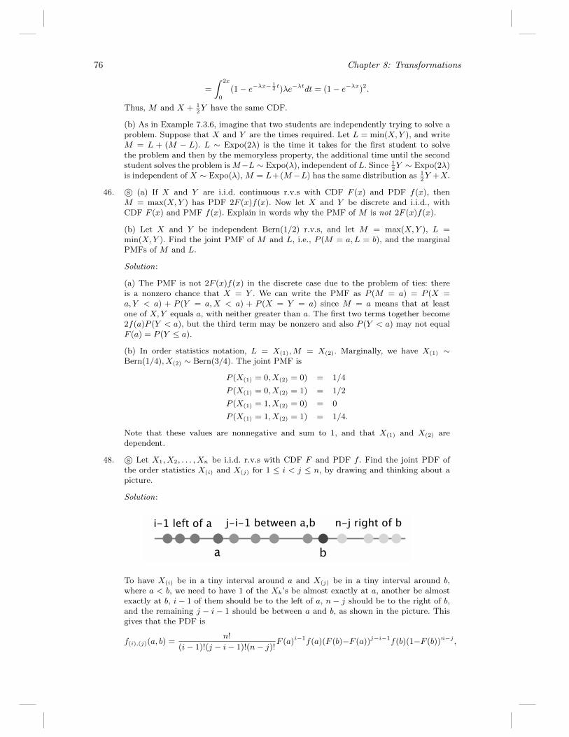
76 Chapter 8: Transformations
=
∫ 2x
0
(1− e−λx−12t)λe−λtdt = (1− e−λx)2.
Thus, M and X + 12Y have the same CDF.
(b) As in Example 7.3.6, imagine that two students are independently trying to solve aproblem. Suppose that X and Y are the times required. Let L = min(X,Y ), and writeM = L + (M − L). L ∼ Expo(2λ) is the time it takes for the first student to solvethe problem and then by the memoryless property, the additional time until the secondstudent solves the problem is M−L ∼ Expo(λ), independent of L. Since 1
2Y ∼ Expo(2λ)
is independent of X ∼ Expo(λ), M = L+(M−L) has the same distribution as 12Y +X.
46. s© (a) If X and Y are i.i.d. continuous r.v.s with CDF F (x) and PDF f(x), thenM = max(X,Y ) has PDF 2F (x)f(x). Now let X and Y be discrete and i.i.d., withCDF F (x) and PMF f(x). Explain in words why the PMF of M is not 2F (x)f(x).
(b) Let X and Y be independent Bern(1/2) r.v.s, and let M = max(X,Y ), L =min(X,Y ). Find the joint PMF of M and L, i.e., P (M = a, L = b), and the marginalPMFs of M and L.
Solution:
(a) The PMF is not 2F (x)f(x) in the discrete case due to the problem of ties: thereis a nonzero chance that X = Y . We can write the PMF as P (M = a) = P (X =a, Y < a) + P (Y = a,X < a) + P (X = Y = a) since M = a means that at leastone of X,Y equals a, with neither greater than a. The first two terms together become2f(a)P (Y < a), but the third term may be nonzero and also P (Y < a) may not equalF (a) = P (Y ≤ a).
(b) In order statistics notation, L = X(1),M = X(2). Marginally, we have X(1) ∼Bern(1/4), X(2) ∼ Bern(3/4). The joint PMF is
P (X(1) = 0, X(2) = 0) = 1/4
P (X(1) = 0, X(2) = 1) = 1/2
P (X(1) = 1, X(2) = 0) = 0
P (X(1) = 1, X(2) = 1) = 1/4.
Note that these values are nonnegative and sum to 1, and that X(1) and X(2) aredependent.
48. s© Let X1, X2, . . . , Xn be i.i.d. r.v.s with CDF F and PDF f . Find the joint PDF ofthe order statistics X(i) and X(j) for 1 ≤ i < j ≤ n, by drawing and thinking about apicture.
Solution:
a b
i-1 left of a n-j right of bj-i-1 between a,b
To have X(i) be in a tiny interval around a and X(j) be in a tiny interval around b,where a < b, we need to have 1 of the Xk’s be almost exactly at a, another be almostexactly at b, i− 1 of them should be to the left of a, n− j should be to the right of b,and the remaining j − i − 1 should be between a and b, as shown in the picture. Thisgives that the PDF is
f(i),(j)(a, b) =n!
(i− 1)!(j − i− 1)!(n− j)!F (a)i−1f(a)(F (b)−F (a))j−i−1f(b)(1−F (b))n−j ,
Chapter 8: Transformations 77
for a < b. The coefficient in front counts the number of ways to put the Xk’s into the 5categories “left of a,” “at a,” “between a and b,” “at b,” “right of b” with the desirednumber in each category (which is the same idea used to find the coefficient in front of theMultinomial PMF). Equivalently, we could write the coefficient as n(n−1)
(n−2i−1
)(n−i−1j−i−1
),
since there are n choices for which Xk is at a, then n− 1 choices for which is at b, etc.
49. s© Two women are pregnant, both with the same due date. On a timeline, define time0 to be the instant when the due date begins. Suppose that the time when the womangives birth has a Normal distribution, centered at 0 and with standard deviation 8 days.Assume that the two birth times are i.i.d. Let T be the time of the first of the two births(in days).
(a) Show that
E(T ) =−8√π.
Hint: For any two random variables X and Y , we have max(X,Y )+min(X,Y ) = X+Yand max(X,Y ) − min(X,Y ) = |X − Y |. Example 7.2.3 derives the expected distancebetween two i.i.d. N (0, 1) r.v.s.
(b) Find Var(T ), in terms of integrals. You can leave your answers unsimplified for thisproblem, but it can be shown that the answer works out to
Var(T ) = 64
(1− 1
π
).
Solution: Let T = min(T1, T2), with T1 and T2 the i.i.d. birth times. Standardizing, let
X =T1
8, Y =
T2
8, L =
T
8,
so X and Y are i.i.d. N (0, 1), and L = min(X,Y ). Also, let
M = max(X,Y ), S = X + Y,W = |X − Y |.
We have M + L = S and M − L = W , so M = 12(S +W ) and L = 1
2(S −W ). Then
E(S) = 0 and E(W ) =2√π,
by Example 7.2.3. Thus,
E(M) =1
2E(W ) =
1√π,E(L) =
−1
2E(W ) =
−1√π.
It follows that
E(T ) = 8E(L) =−8√π.
(b) We can find the PDF of T using order statistics results, or directly using
P (T > t) = P (T1 > t, T2 > t) = (1− Φ(t/8))2.
So the PDF of T is
f(t) =1
4(1− Φ(t/8))ϕ(t/8),
where ϕ(z) = 1√2πe−z
2/2 is the N (0, 1) PDF. Thus,
Var(T ) =
∫ ∞−∞
t2f(t)dt−(∫ ∞−∞
tf(t)dt
)2
,
78 Chapter 8: Transformations
with f as above.
To get the variance in closed form (which was not requested in the problem), note that(with notation as above) X+Y and X−Y are independent since they are uncorrelatedand (X + Y,X − Y ) is MVN. So S = X + Y and W = |X − Y | are independent. Thus,
Var(L) =1
4(Var(S) + Var(W )).
We have Var(S) = 2, and
Var(W ) = E(X − Y )2 − (E(W ))2 = Var(X − Y )− (E(W ))2 = 2− 4
π.
Therefore,
Var(L) = 1− 1
π,
which shows that
Var(T ) = 64
(1− 1
π
).
Mixed practice
53. s© A DNA sequence can be represented as a sequence of letters, where the “alphabet”has 4 letters: A,C,T,G. Suppose such a sequence is generated randomly, where the lettersare independent and the probabilities of A,C,T,G are p1, p2, p3, p4 respectively.
(a) In a DNA sequence of length 115, what is the expected number of occurrences ofthe expression “CATCAT” (in terms of the pj)? (Note that, for example, the expression“CATCATCAT” counts as 2 occurrences.)
(b) What is the probability that the first A appears earlier than the first C appears, asletters are generated one by one (in terms of the pj)?
(c) For this part, assume that the pj are unknown. Suppose we treat p2 as a Unif(0, 1)r.v. before observing any data, and that then the first 3 letters observed are “CAT”.Given this information, what is the probability that the next letter is C?
Solution:
(a) Let Ij be the indicator r.v. of “CATCAT” appearing starting at position j, for1 ≤ j ≤ 110. Then E(Ij) = (p1p2p3)2, so the expected number is 110(p1p2p3)2.
Sanity check : The number of occurrences is between 0 and 110, so the expected valuemust also be between 0 and 110. If any of the letters C, A, or T is very rare, then“CATCAT” will be even more rare; this is reflected in the p2j factors, which will makethe expected number small if any of p1, p2, p3 is small.
(b) Consider the first letter which is an A or a C (call it X; alternatively, condition onthe first letter of the sequence). This gives
P (A before C) = P (X is A|X is A or C) =P (X is A)
P (X is A or C)=
p1p1 + p2
.
Sanity check : The answer should be 1/2 for p1 = p2, should go to 0 as p1 → 0, should beincreasing in p1 and decreasing in p2, and finding P (A before C) by 1− P (A before C)should agree with finding it by swapping p1, p2.
(c) Let X be the number of C’s in the data (so X = 1 is observed here). The prior isp2 ∼ Beta(1, 1), so the posterior is p2|X = 1 ∼ Beta(2, 3) (by the connection betweenBeta and Binomial, or by Bayes’ Rule). Given p2, the indicator of the next letter being
Chapter 8: Transformations 79
C is Bern(p2). So given X (but not given p2), the probability of the next letter being Cis E(p2|X) = 2
5.
Sanity check : It makes sense that the answer should be strictly in between 1/2 (themean of the prior distribution) and 1/3 (the observed frequency of C’s in the data).
54. s© Consider independent Bernoulli trials with probability p of success for each. Let Xbe the number of failures incurred before getting a total of r successes.
(a) Determine what happens to the distribution of p1−pX as p→ 0, using MGFs; what
is the PDF of the limiting distribution, and its name and parameters if it is one we havestudied?
Hint: Start by finding the Geom(p) MGF. Then find the MGF of p1−pX, and use the
fact that if the MGFs of r.v.s Yn converge to the MGF of an r.v. Y , then the CDFs ofthe Yn converge to the CDF of Y .
(b) Explain intuitively why the result of (a) makes sense.
Solution:
(a) Let q = 1− p. For G ∼ Geom(p), the MGF is
E(etG) = p
∞∑k=0
etkqk = p
∞∑k=0
(qet)k =p
1− qet ,
for qet < 1. So the NBin(r, p) MGF is pr
(1−qet)r for qet < 1. Then the MGF of p1−pX is
E(etpqX
) =pr
(1− qetp/q)r
for qetp/q < 1. Let us first consider the limit for r = 1. As p → 0, the numerator goesto 0 and so does the denominator (since qetp/q → 1e0 = 1). By L’Hopital’s Rule,
limp→0
p
1− (1− p)etp/(1−p)= limp→0
1
etp/(1−p) − (1− p)t(
1−p+p(1−p)2
)etp/(1−p)
=1
1− t .
So for any fixed r > 0, as p→ 0 we have
E(etpqX)
=pr
(1− qetp/q)r→ 1
(1− t)r .
This is the Gamma(r, 1) MGF for t < 1 (note also that the condition qetp/q < 1 isequivalent to t < − 1−p
plog(1−p), which converges to the condition t < 1 since again by
L’Hopital’s Rule, −plog(1−p) → 1). Thus, the scaled Negative Binomial p
1−pX converges to
Gamma(r, 1) in distribution as p→ 0.
(b) The result of (a) makes sense intuitively since the Gamma is the continuous analogueof the Negative Binomial, just as the Exponential is the continuous analog of the Geo-metric. To convert from discrete to continuous, imagine performing many, many trialswhere each is performed very, very quickly and has a very, very low chance of success.To balance the rate of trials with the chance of success, we use the scaling p
qsince this
makes E( pqX) = r, matching the Gamma(r, 1) mean.

Chapter 9: Conditional expectation
Conditional expectation given an event
7. s© You get to choose between two envelopes, each of which contains a check for somepositive amount of money. Unlike in the two-envelope paradox, it is not given that oneenvelope contains twice as much money as the other envelope. Instead, assume that thetwo values were generated independently from some distribution on the positive realnumbers, with no information given about what that distribution is.
After picking an envelope, you can open it and see how much money is inside (call thisvalue x), and then you have the option of switching. As no information has been givenabout the distribution, it may seem impossible to have better than a 50% chance ofpicking the better envelope. Intuitively, we may want to switch if x is “small” and notswitch if x is “large”, but how do we define “small” and “large” in the grand scheme ofall possible distributions? [The last sentence was a rhetorical question.]
Consider the following strategy for deciding whether to switch. Generate a thresholdT ∼ Expo(1), and switch envelopes if and only if the observed value x is less than thevalue of T . Show that this strategy succeeds in picking the envelope with more moneywith probability strictly greater than 1/2.
Hint: Let t be the value of T (generated by a random draw from the Expo(1) distribu-tion). First explain why the strategy works very well if t happens to be in between thetwo envelope values, and does no harm in any case (i.e., there is no case in which thestrategy succeeds with probability strictly less than 1/2).
Solution: Let a be the smaller value of the two envelopes and b be the larger value(assume a < b since in the case a = b it makes no difference which envelope is chosen!).Let G be the event that the strategy succeeds and A be the event that we pick theenvelope with a initially. Then P (G|A) = P (T > a) = 1 − (1 − e−a) = e−a, andP (G|Ac) = P (T ≤ b) = 1− e−b. Thus, the probability that the strategy succeeds is
1
2e−a +
1
2(1− e−b) =
1
2+
1
2(e−a − e−b) > 1
2,
because e−a − e−b > 0.
10. s© A coin with probability p of Heads is flipped repeatedly. For (a) and (b), supposethat p is a known constant, with 0 < p < 1.
(a) What is the expected number of flips until the pattern HT is observed?
(b) What is the expected number of flips until the pattern HH is observed?
(c) Now suppose that p is unknown, and that we use a Beta(a, b) prior to reflect ouruncertainty about p (where a and b are known constants and are greater than 2). Interms of a and b, find the corresponding answers to (a) and (b) in this setting.
Solution:
(a) This can be thought of as “Wait for Heads, then wait for the first Tails after thefirst Heads,” so the expected value is 1
p+ 1
q, with q = 1− p.
81
82 Chapter 9: Conditional expectation
(b) Let X be the waiting time for HH and condition on the first toss, writing H for theevent that the first toss is Heads and T for the complement of H:
E(X) = E(X|H)p+ E(X|T )q = E(X|H)p+ (1 + EX)q.
To find E(X|H), condition on the second toss:
E(X|H) = E(X|HH)p+ E(X|HT )q = 2p+ (2 + EX)q.
Solving for E(X), we have
E(X) =1
p+
1
p2.
Sanity check : This gives E(X) = 6 when p = 1/2, in agreement with Example 9.1.9.
(c) Let X and Y be the number of flips until HH and until HT , respectively. By(a), E(Y |p) = 1
p+ 1
1−p . So E(Y ) = E(E(Y |p)) = E( 1p) + E( 1
1−p ). Likewise, by (b),
E(X) = E(E(X|p)) = E( 1p) + E( 1
p2). By LOTUS,
E
(1
p
)=
Γ(a+ b)
Γ(a)Γ(b)
∫ 1
0
pa−2(1− p)b−1dp =Γ(a+ b)
Γ(a)Γ(b)
Γ(a− 1)Γ(b)
Γ(a+ b− 1)=a+ b− 1
a− 1,
E
(1
1− p
)=
Γ(a+ b)
Γ(a)Γ(b)
∫ 1
0
pa−1(1− p)b−2dp =Γ(a+ b)
Γ(a)Γ(b)
Γ(a)Γ(b− 1)
Γ(a+ b− 1)=a+ b− 1
b− 1,
E
(1
p2
)=
Γ(a+ b)
Γ(a)Γ(b)
∫ 1
0
pa−3(1−p)b−1dp =Γ(a+ b)
Γ(a)Γ(b)
Γ(a− 2)Γ(b)
Γ(a+ b− 2)=
(a+ b− 1)(a+ b− 2)
(a− 1)(a− 2).
Thus,
E(Y ) =a+ b− 1
a− 1+a+ b− 1
b− 1,
E(X) =a+ b− 1
a− 1+
(a+ b− 1)(a+ b− 2)
(a− 1)(a− 2).
Conditional expectation given a random variable
13. s© Let X1, X2 be i.i.d., and let X = 12(X1 +X2) be the sample mean. In many statistics
problems, it is useful or important to obtain a conditional expectation given X. As anexample of this, find E(w1X1 +w2X2|X), where w1, w2 are constants with w1 +w2 = 1.
Solution: By symmetry E(X1|X) = E(X2|X) and by linearity and taking out what’sknown, E(X1|X)+E(X2|X) = E(X1+X2|X) = X1+X2. So E(X1|X) = E(X2|X) = X(see also Example 9.3.6). Thus,
E(w1X1 + w2X2|X) = w1E(X1|X) + w2E(X2|X) = w1X + w2X = X.
15. s© Consider a group of n roommate pairs at a college (so there are 2n students). Eachof these 2n students independently decides randomly whether to take a certain course,with probability p of success (where “success” is defined as taking the course).
Let N be the number of students among these 2n who take the course, and let X bethe number of roommate pairs where both roommates in the pair take the course. FindE(X) and E(X|N).
Solution: Create an indicator r.v. Ij for the jth roommate pair, equal to 1 if bothtake the course. The expected value of such an indicator r.v. is p2, so E(X) = np2 bysymmetry and linearity. Similarly, E(X|N) = nE(I1|N). We have
E(I1|N) =N
2n
N − 1
2n− 1
Chapter 9: Conditional expectation 83
since given that N of the 2n students take the course, the probability is N2n
that anyparticular student takes Stat 110 (the p no longer matters), and given that one particularstudent in a roommate pair takes the course, the probability that the other roommate
does is N−12n−1
. Or write E(I1|N) =(N2 )(2n2 )
, since given N , the number of students in the
first roommate pair who are in the course is Hypergeometric! Thus,
E(X|N) = nE(I1|N) =N(N − 1)
2
1
2n− 1.
Historical note: an equivalent problem was first solved in the 1760s by Daniel Bernoulli, anephew of Jacob Bernoulli. (The Bernoulli distribution is named after Jacob Bernoulli.)
16. s© Show that E((Y −E(Y |X))2|X) = E(Y 2|X)− (E(Y |X))2, so these two expressionsfor Var(Y |X) agree.
Solution: This is the conditional version of the fact that
Var(Y ) = E((Y − E(Y ))2) = E(Y 2)− (E(Y ))2,
and so must be true since conditional expectations are expectations, just as conditionalprobabilities are probabilities. Algebraically, letting g(X) = E(Y |X) we have
E((Y−E(Y |X))2|X) = E(Y 2−2Y g(X)+g(X)2|X) = E(Y 2|X)−2E(Y g(X)|X)+E(g(X)2|X),
and E(Y g(X)|X) = g(X)E(Y |X) = g(X)2, E(g(X)2|X) = g(X)2 by taking out what’sknown, so the righthand side above simplifies to E(Y 2|X)− g(X)2.
22. s© Let X and Y be random variables with finite variances, and let W = Y − E(Y |X).This is a residual : the difference between the true value of Y and the predicted value ofY based on X.
(a) Compute E(W ) and E(W |X).
(b) Compute Var(W ), for the case that W |X ∼ N (0, X2) with X ∼ N (0, 1).
Solution:
(a) Adam’s law, taking out what’s known, and linearity give
E(W ) = EY − E(E(Y |X)) = EY − EY = 0,
E(W |X) = E(Y |X)− E(E(Y |X)|X) = E(Y |X)− E(Y |X) = 0.
(b) Eve’s Law gives
Var(W ) = Var(E(W |X)) + E(Var(W |X)) = Var(0) + E(X2) = 0 + 1 = 1.
23. s© One of two identical-looking coins is picked from a hat randomly, where one coin hasprobability p1 of Heads and the other has probability p2 of Heads. Let X be the numberof Heads after flipping the chosen coin n times. Find the mean and variance of X.
Solution: The distribution of X is a mixture of two Binomials; this is not Binomialunless p1 = p2. Let I be the indicator of having the p1 coin. Then
E(X) = E(X|I = 1)P (I = 1) + E(X|I = 0)P (I = 0) =1
2n(p1 + p2).
Alternatively, we can represent X as X = IX1 + (1 − I)X2 with Xj ∼ Bin(n, pj), andI,X1, X2 independent. Then
E(X) = E(E(X|I)) = E(Inp1 + (1− I)np2) =1
2n(p1 + p2).
84 Chapter 9: Conditional expectation
For the variance, note that it is not valid to say “Var(X) = Var(X|I = 1)P (I =1) + Var(X|I = 0)P (I = 0)”; an extreme example of this mistake would be claimingthat “Var(I) = 0 since Var(I|I = 1)P (I = 1) + Var(I|I = 0)P (I = 0) = 0”; of course,Var(I) = 1
4). Instead, we can use Eve’s Law:
Var(X) = E(Var(X|I)) + Var(E(X|I)),
where Var(X|I) = Inp1(1− p1) + (1− I)np2(1− p2) is np1(1− p1) with probability 1/2and np2(1 − p2) with probability 1/2, and E(X|I) = Inp1 + (1 − I)np2 is np1 or np2with probability 1
2each, so
Var(X) =1
2(np1(1− p1) + np2(1− p2)) +
1
4n2(p1 − p2)2.
27. s© We wish to estimate an unknown parameter θ, based on an r.v. X we will get toobserve. As in the Bayesian perspective, assume that X and θ have a joint distribution.Let θ be the estimator (which is a function of X). Then θ is said to be unbiased ifE(θ|θ) = θ, and θ is said to be the Bayes procedure if E(θ|X) = θ.
(a) Let θ be unbiased. Find E(θ − θ)2 (the average squared difference between theestimator and the true value of θ), in terms of marginal moments of θ and θ.
Hint: Condition on θ.
(b) Repeat (a), except in this part suppose that θ is the Bayes procedure rather thanassuming that it is unbiased.
Hint: Condition on X.
(c) Show that it is impossible for θ to be both the Bayes procedure and unbiased, exceptin silly problems where we get to know θ perfectly by observing X.
Hint: If Y is a nonnegative r.v. with mean 0, then P (Y = 0) = 1.
Solution:
(a) Conditioning on θ, we have
E(θ − θ)2 = E(E(θ2 − 2θθ + θ2|θ))
= E(E(θ2|θ))− E(E(2θθ|θ)) + E(E(θ2|θ))
= E(θ2)− 2E(θE(θ|θ)) + E(θ2)
= E(θ2)− 2E(θ2) + E(θ2)
= E(θ2)− E(θ2).
(b) By the same argument as for (a) except now conditioning on X, we have
E(θ − θ)2 = E(E(θ2 − 2θθ + θ2|X))
= E(E(θ2|X))− E(E(2θθ|X)) + E(E(θ2|X))
= E(θ2)− 2E(θ2) + E(θ2)
= E(θ2)− E(θ2).
(c) Suppose that θ is both the Bayes procedure and unbiased. By the above, we haveE(θ − θ)2 = a and E(θ − θ)2 = −a, where a = E(θ2)− E(θ2). But that implies a = 0,which means that θ = θ (with probability 1). That can only happen in the extremesituation where the observed data reveal the true θ perfectly ; in practice, nature is muchmore elusive and does not reveal its deepest secrets with such alacrity.
Chapter 9: Conditional expectation 85
30. s© Emails arrive one at a time in an inbox. Let Tn be the time at which the nth emailarrives (measured on a continuous scale from some starting point in time). Suppose thatthe waiting times between emails are i.i.d. Expo(λ), i.e., T1, T2−T1, T3−T2, . . . are i.i.d.Expo(λ).
Each email is non-spam with probability p, and spam with probability q = 1 − p (in-dependently of the other emails and of the waiting times). Let X be the time at whichthe first non-spam email arrives (so X is a continuous r.v., with X = T1 if the 1st emailis non-spam, X = T2 if the 1st email is spam but the 2nd one isn’t, etc.).
(a) Find the mean and variance of X.
(b) Find the MGF of X. What famous distribution does this imply that X has (be sureto state its parameter values)?
Hint for both parts: Let N be the number of emails until the first non-spam (includingthat one), and write X as a sum of N terms; then condition on N .
Solution:
(a) Write X = X1 +X2 + · · ·+XN , where Xj is the time from the (j − 1)th to the jthemail for j ≥ 2, and X1 = T1. Then N − 1 ∼ Geom(p), so
E(X) = E(E(X|N)) = E(N1
λ) =
1
pλ.
And
Var(X) = E(Var(X|N)) + Var(E(X|N)) = E(N1
λ2) + Var(N
1
λ),
which is1
pλ2+
1− pp2λ2
=1
p2λ2.
(b) Again conditioning on N , the MGF is
E(etX) = E(E(etX1etX2 · · · etXN |N)) = E(E(etX1 |N)E(etX2 |N) . . . E(etXN |N)
)= E(M1(t)N ),
where M1(t) is the MGF of X1 (which is λλ−t for t < λ). By LOTUS, this is
p
∞∑n=1
M1(t)nqn−1 =p
q
∞∑n=1
(qM1(t))n =p
q
qM1(t)
1− qM1(t)=
pλλ−t
1− qλλ−t
=pλ
pλ− t
for t < pλ (as we need qM1(t) < 1 for the series to converge). This is the Expo(pλ)MGF, so X ∼ Expo(pλ).
33. s© Judit plays in a total of N ∼ Geom(s) chess tournaments in her career. Suppose thatin each tournament she has probability p of winning the tournament, independently.Let T be the number of tournaments she wins in her career.
(a) Find the mean and variance of T .
(b) Find the MGF of T . What is the name of this distribution (with its parameters)?
Solution:
(a) We have T |N ∼ Bin(N, p). By Adam’s Law,
E(T ) = E(E(T |N)) = E(Np) = p(1− s)/s.
86 Chapter 9: Conditional expectation
By Eve’s Law,
Var(T ) = E(Var(T |N)) + Var(E(T |N))
= E(Np(1− p)) + Var(Np)
= p(1− p)(1− s)/s+ p2(1− s)/s2
=p(1− s)(s+ (1− s)p)
s2.
(b) Let Ij ∼ Bern(p) be the indicator of Judit winning the jth tournament. Then
E(etT ) = E(E(etT |N))
= E((pet + q)N )
= s
∞∑n=0
(pet + 1− p)n(1− s)n
=s
1− (1− s)(pet + 1− p) .
This is reminiscent of the Geometric MGF, which was derived in Example 6.4.3. IfT ∼ Geom(θ), we have θ = s
s+p(1−s) , as found by setting E(T ) = 1−θθ
or by finding
Var(T )/E(T ). Writing the MGF of T as
E(etT ) =s
s+ (1− s)p− (1− s)pet =
ss+(1−s)p
1− (1−s)ps+(1−s)pe
t,
we see that T ∼ Geom(θ), with θ = ss+(1−s)p . Note that this is consistent with (a).
The distribution of T can also be obtained by a story proof. Imagine that just beforeeach tournament she may play in, Judit retires with probability s (if she retires, shedoes not play in that or future tournaments). Her tournament history can be written asa sequence of W (win), L (lose), R (retire), ending in the first R, where the probabilitiesof W,L,R are (1 − s)p, (1 − s)(1 − p), s respectively. For calculating T , the losses canbe ignored: we want to count the number of W ’s before the R. The probability that aresult is R given that it is W or R is s
s+(1−s)p , so we again have
T ∼ Geom(s
s+ (1− s)p ).
36. s© A certain stock has low volatility on some days and high volatility on other days.Suppose that the probability of a low volatility day is p and of a high volatility dayis q = 1 − p, and that on low volatility days the percent change in the stock price isN (0, σ2
1), while on high volatility days the percent change is N (0, σ22), with σ1 < σ2.
Let X be the percent change of the stock on a certain day. The distribution is said tobe a mixture of two Normal distributions, and a convenient way to represent X is asX = I1X1+I2X2 where I1 is the indicator r.v. of having a low volatility day, I2 = 1−I1,Xj ∼ N (0, σ2
j ), and I1, X1, X2 are independent.
(a) Find Var(X) in two ways: using Eve’s law, and by calculating Cov(I1X1 +I2X2, I1X1 + I2X2) directly.
(b) Recall from Chapter 6 that the kurtosis of an r.v. Y with mean µ and standarddeviation σ is defined by
Kurt(Y ) =E(Y − µ)4
σ4− 3.
Find the kurtosis of X (in terms of p, q, σ21 , σ
22 , fully simplified). The result will show that
Chapter 9: Conditional expectation 87
even though the kurtosis of any Normal distribution is 0, the kurtosis of X is positiveand in fact can be very large depending on the parameter values.
Solution:
(a) By Eve’s Law,
Var(X) = E(Var(X|I1))+Var(E(X|I1)) = E(I21σ21+(1−I1)2σ2
2)+Var(0) = pσ21+(1−p)σ2
2 ,
since I21 = I1, I22 = I2. For the covariance method, expand
Var(X) = Cov(I1X1+I2X2, I1X1+I2X2) = Var(I1X1)+Var(I2X2)+2Cov(I1X1, I2X2).
Then Var(I1X1) = E(I21X21 )− (E(I1X1))2 = E(I1)E(X2
1 ) = pVar(X1) since E(I1X1) =E(I1)E(X1) = 0. Similarly, Var(I2X2) = (1− p)Var(X2). And
Cov(I1X1, I2X2) = E(I1I2X1X2)− E(I1X1)E(I2X2) = 0,
since I1I2 always equals 0. So again we have Var(X) = pσ21 + (1− p)σ2
2 .
(b) Note that (I1X1 + I2X2)4 = I1X41 + I2X
42 since the cross terms disappear (because
I1I2 is always 0) and any positive power of an indicator r.v. is that indicator r.v.! So
E(X4) = E(I1X41 + I2X
42 ) = 3pσ4
1 + 3qσ42 .
Alternatively, we can use E(X4) = E(X4|I1 = 1)p+E(X4|I1 = 0)q to find E(X4). Themean of X is E(I1X1) + E(I2X2) = 0, so the kurtosis of X is
Kurt(X) =3pσ4
1 + 3qσ42
(pσ21 + qσ2
2)2− 3.
This becomes 0 if σ1 = σ2, since then we have a Normal distribution rather than amixture of two different Normal distributions. For σ1 < σ2, the kurtosis is positive since
pσ41 + qσ4
2 > (pσ21 + qσ2
2)2,
as can be seen by interpreting this as saying E(Y 2) > (EY )2, where Y is σ21 with
probability p and σ22 with probability q.
Mixed practice
43. s© Empirically, it is known that 49% of children born in the U.S. are girls (and 51% areboys). Let N be the number of children who will be born in the U.S. in March of nextyear, and assume that N is a Pois(λ) random variable, where λ is known. Assume thatbirths are independent (e.g., don’t worry about identical twins).
Let X be the number of girls who will be born in the U.S. in March of next year, andlet Y be the number of boys who will be born then.
(a) Find the joint distribution of X and Y . (Give the joint PMF.)
(b) Find E(N |X) and E(N2|X).
Solution:
(a) By the chicken-egg story, X and Y are independent with X ∼ Pois(0.49λ), Y ∼Pois(0.51λ). The joint PMF is
P (X = i, Y = j) = (e−0.49λ(0.49λ)i/i!)(e−0.51λ(0.51λ)j/j!).
(b) Since X and Y are independent,
E(N |X) = E(X + Y |X) = X + E(Y |X) = X + EY = X + 0.51λ,
E(N2|X) = E(X2 + 2XY + Y 2|X) = X2 + 2XE(Y ) +E(Y 2) = (X + 0.51λ)2 + 0.51λ.
88 Chapter 9: Conditional expectation
44. s© Let X1, X2, X3 be independent with Xi ∼ Expo(λi) (so with possibly different rates).Recall from Chapter 7 that
P (X1 < X2) =λ1
λ1 + λ2.
(a) Find E(X1 +X2 +X3|X1 > 1, X2 > 2, X3 > 3) in terms of λ1, λ2, λ3.
(b) Find P (X1 = min(X1, X2, X3)), the probability that the first of the three Exponen-tials is the smallest.
Hint: Restate this in terms of X1 and min(X2, X3).
(c) For the case λ1 = λ2 = λ3 = 1, find the PDF of max(X1, X2, X3). Is this one of theimportant distributions we have studied?
Solution:
(a) By linearity, independence, and the memoryless property, we get
E(X1|X1 > 1) + E(X2|X2 > 2) + E(X3|X3 > 3) = λ−11 + λ−1
2 + λ−13 + 6.
(b) The desired probability is P (X1 ≤ min(X2, X3)). Noting that min(X2, X3) ∼Expo(λ2 + λ3) is independent of X1, we have
P (X1 ≤ min(X2, X3)) =λ1
λ1 + λ2 + λ3.
(c) Let M = max(X1, X2, X3). Using the order statistics results from class or by directlycomputing the CDF and taking the derivative, for x > 0 we have
fM (x) = 3(1− e−x)2e−x.
This is not one of the important distributions we have studied. The form is reminiscentof a Beta, but a Beta takes values between 0 and 1, while M can take any positive realvalue (in fact, B ∼ Beta(1, 3) if we make the transformation B = e−M .)
45. s© A task is randomly assigned to one of two people (with probability 1/2 for eachperson). If assigned to the first person, the task takes an Expo(λ1) length of timeto complete (measured in hours), while if assigned to the second person it takes anExpo(λ2) length of time to complete (independent of how long the first person wouldhave taken). Let T be the time taken to complete the task.
(a) Find the mean and variance of T .
(b) Suppose instead that the task is assigned to both people, and let X be the timetaken to complete it (by whoever completes it first, with the two people working in-dependently). It is observed that after 24 hours, the task has not yet been completed.Conditional on this information, what is the expected value of X?
Solution: Write T = IX1 + (1 − I)X2, with I ∼ Bern(1/2), X1 ∼ Expo(λ1), X2 ∼Expo(λ2) independent. Then
ET =1
2(λ−1
1 + λ−12 ),
Var(T ) = E(Var(T |I)) + Var(E(T |I))
= E(I21
λ21
+ (1− I)21
λ22
) + Var
(I
λ1+
1− Iλ2
)= E(I
1
λ21
+ (1− I)1
λ22
) + Var
(I(
1
λ1− 1
λ2)
)=
1
2(
1
λ21
+1
λ22
) +1
4(
1
λ1− 1
λ2)2.
Chapter 9: Conditional expectation 89
Sanity check : For λ1 = λ2, the two people have the same distribution so randomlyassigning the task to one of the two should be equivalent to just assigning it to the firstperson (so the mean and variance should agree with those of an Expo(λ1) r.v.). It makessense that the mean is the average of the two means, as we can condition on whetherI = 1 (though the variance is greater than the average of the two variances, by Eve’sLaw). Also, the results should be (and are) the same if we swap λ1 and λ2.
(b) Here X = min(X1, X2) with X1 ∼ Expo(λ1), X2 ∼ Expo(λ2) independent. ThenX ∼ Expo(λ1 + λ2) (since P (X > x) = P (X1 > x)P (X2 > x) = e−(λ1+λ2)x, or byresults on order statistics). By the memoryless property,
E(X|X > 24) = 24 +1
λ1 + λ2.
Sanity check : The answer should be greater than 24 and should be very close to 24 ifλ1 or λ2 is very large. Considering a Poisson process also helps make this intuitive.
47. s© A certain genetic characteristic is of interest. It can be measured numerically. Let X1
and X2 be the values of the genetic characteristic for two twin boys. If they are identicaltwins, then X1 = X2 and X1 has mean 0 and variance σ2; if they are fraternal twins,then X1 and X2 have mean 0, variance σ2, and correlation ρ. The probability that thetwins are identical is 1/2. Find Cov(X1, X2) in terms of ρ, σ2.
Solution: Since the means are 0, Cov(X1, X2) = E(X1X2)− (EX1)(EX2) = E(X1X2).Now condition on whether the twins are identical or fraternal:
E(X1X2) = E(X1X2|identical)1
2+E(X1X2|fraternal)
1
2= E(X2
1 )1
2+ρσ2 1
2=σ2
2(1+ρ).
48. s© The Mass Cash lottery randomly chooses 5 of the numbers from 1, 2, . . . , 35 each day(without repetitions within the choice of 5 numbers). Suppose that we want to knowhow long it will take until all numbers have been chosen. Let aj be the average numberof additional days needed if we are missing j numbers (so a0 = 0 and a35 is the averagenumber of days needed to collect all 35 numbers). Find a recursive formula for the aj .
Solution: Suppose we are missing j numbers (with 0 ≤ j ≤ 35), and let Tj be theadditional number of days needed to complete the collection. Condition on how many“new” numbers appear the next day; call this N . This gives
E(Tj) =
5∑n=0
E(Tj |N = n)P (N = n).
Note that N is Hypergeometric (imagine tagging the numbers that we don’t alreadyhave in our collection)! Letting ak = 0 for k < 0, we have
aj = 1 +
5∑n=0
aj−n(jn
)(35−j5−n
)(355
) .

Chapter 10: Inequalities and limittheorems
Inequalities
1. s© In a national survey, a random sample of people are chosen and asked whether theysupport a certain policy. Assume that everyone in the population is equally likely tobe surveyed at each step, and that the sampling is with replacement (sampling withoutreplacement is typically more realistic, but with replacement will be a good approxima-tion if the sample size is small compared to the population size). Let n be the samplesize, and let p and p be the proportion of people who support the policy in the sampleand in the entire population, respectively. Show that for every c > 0,
P (|p− p| > c) ≤ 1
4nc2.
Solution: We can write p = X/n with X ∼ Bin(n, p). So E(p) = p,Var(p) = p(1− p)/n.Then by Chebyshev’s inequality,
P (|p− p| > c) ≤ Var(p)
c2=p(1− p)nc2
≤ 1
4nc2,
where the last inequality is because p(1− p) is maximized at p = 1/2.
2. s© For i.i.d. r.v.s X1, . . . , Xn with mean µ and variance σ2, give a value of n (as a specificnumber) that will ensure that there is at least a 99% chance that the sample mean willbe within 2 standard deviations of the true mean µ.
Solution: We have to find n such that
P (|Xn − µ| > 2σ) ≤ 0.01.
By Chebyshev’s inequality (in the form P (|Y − EY | > c) ≤ Var(Y )
c2), we have
P (|Xn − µ| > 2σ) ≤ VarXn(2σ)2
=σ2
n
4σ2=
1
4n.
So the desired inequality holds if n ≥ 25.
3. s© Show that for any two positive r.v.s X and Y with neither a constant multiple of theother,
E(X/Y )E(Y/X) > 1.
Solution: The r.v. W = Y/X is positive and non-constant, so Jensen’s inequality yields
E(X/Y ) = E(1/W ) > 1/E(W ) = 1/E(Y/X).
4. s© The famous arithmetic mean-geometric mean inequality says that for any positivenumbers a1, a2, . . . , an,
a1 + a2 + · · ·+ ann
≥ (a1a2 · · · an)1/n.
91
92 Chapter 10: Inequalities and limit theorems
Show that this inequality follows from Jensen’s inequality, by considering E log(X) foran r.v. X whose possible values are a1, . . . , an (you should specify the PMF of X; if youwant, you can assume that the aj are distinct (no repetitions), but be sure to say so ifyou assume this).
Solution: Assume that the aj are distinct, and let X be a random variable which takesvalues from a1, a2, ..., an with equal probability (the case of repeated aj ’s can be handledsimilarly, letting the probability of X = aj be mj/n, where mj is the number of times ajappears in the list a1, . . . , an). Jensen’s inequality gives E(logX) ≤ log(EX), since thelog function is concave. The left-hand side is 1
n
∑ni=1 log ai, while the right hand-side is
log a1+a2+···+ann
. So we have the following inequality:
loga1 + a2 + · · ·+ an
n≥ 1
n
n∑i=1
log ai
Thus,a1 + a2 + · · ·+ an
n≥ e
1n
∑ni=1 log ai = e
log(a1···an)n = (a1 · · · an)1/n.
5. s© Let X be a discrete r.v. whose distinct possible values are x0, x1, . . . , and let pk =P (X = xk). The entropy of X is H(X) =
∑∞k=0 pk log2(1/pk).
(a) Find H(X) for X ∼ Geom(p).
Hint: Use properties of logs, and interpret part of the sum as an expected value.
(b) Let X and Y be i.i.d. discrete r.v.s. Show that P (X = Y ) ≥ 2−H(X).
Hint: Consider E(log2(W )), where W is an r.v. taking value pk with probability pk.
Solution:
(a) We have
H(X) = −∞∑k=0
(pqk) log2(pqk)
= − log2(p)
∞∑k=0
pqk − log2(q)
∞∑k=0
kpqk
= − log2(p)− q
plog2(q),
with q = 1− p, since the first series is the sum of a Geom(p) PMF and the second seriesis the expected value of a Geom(p) r.v.
(b) Let W be as in the hint. By Jensen, E(log2(W )) ≤ log2(EW ). But
E(log2(W )) =∑k
pk log2(pk) = −H(X),
EW =∑k
p2k = P (X = Y ),
so −H(X) ≤ log2 P (X = Y ). Thus, P (X = Y ) ≥ 2−H(X).
Fill-in-the-blank inequalities
7. s© Let X and Y be i.i.d. positive r.v.s, and let c > 0. For each part below, fill in theappropriate equality or inequality symbol: write = if the two sides are always equal,
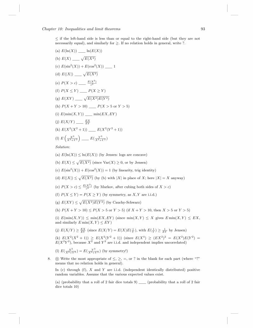
Chapter 10: Inequalities and limit theorems 93
≤ if the left-hand side is less than or equal to the right-hand side (but they are notnecessarily equal), and similarly for ≥. If no relation holds in general, write ?.
(a) E(ln(X)) ln(E(X))
(b) E(X)√E(X2)
(c) E(sin2(X)) + E(cos2(X)) 1
(d) E(|X|)√E(X2)
(e) P (X > c) E(X3)
c3
(f) P (X ≤ Y ) P (X ≥ Y )
(g) E(XY )√E(X2)E(Y 2)
(h) P (X + Y > 10) P (X > 5 or Y > 5)
(i) E(min(X,Y )) min(EX,EY )
(j) E(X/Y ) EXEY
(k) E(X2(X2 + 1)) E(X2(Y 2 + 1))
(l) E(
X3
X3+Y 3
)E( Y 3
X3+Y 3 )
Solution:
(a) E(ln(X)) ≤ ln(E(X)) (by Jensen: logs are concave)
(b) E(X) ≤√E(X2) (since Var(X) ≥ 0, or by Jensen)
(c) E(sin2(X)) + E(cos2(X)) = 1 (by linearity, trig identity)
(d) E(|X|) ≤√E(X2) (by (b) with |X| in place of X; here |X| = X anyway)
(e) P (X > c) ≤ E(X3)
c3(by Markov, after cubing both sides of X > c)
(f) P (X ≤ Y ) = P (X ≥ Y ) (by symmetry, as X,Y are i.i.d.)
(g) E(XY ) ≤√E(X2)E(Y 2) (by Cauchy-Schwarz)
(h) P (X + Y > 10) ≤ P (X > 5 or Y > 5) (if X + Y > 10, then X > 5 or Y > 5)
(i) E(min(X,Y )) ≤ min(EX,EY ) (since min(X,Y ) ≤ X gives Emin(X,Y ) ≤ EX,and similarly Emin(X,Y ) ≤ EY )
(j) E(X/Y ) ≥ EXEY
(since E(X/Y ) = E(X)E( 1Y
), with E( 1Y
) ≥ 1EY
by Jensen)
(k) E(X2(X2 + 1)) ≥ E(X2(Y 2 + 1)) (since E(X4) ≥ (EX2)2 = E(X2)E(Y 2) =E(X2Y 2), because X2 and Y 2 are i.i.d. and independent implies uncorrelated)
(l) E( X3
X3+Y 3 ) = E( Y 3
X3+Y 3 ) (by symmetry!)
8. s© Write the most appropriate of ≤, ≥, =, or ? in the blank for each part (where “?”means that no relation holds in general).
In (c) through (f), X and Y are i.i.d. (independent identically distributed) positiverandom variables. Assume that the various expected values exist.
(a) (probability that a roll of 2 fair dice totals 9) (probability that a roll of 2 fairdice totals 10)

94 Chapter 10: Inequalities and limit theorems
(b) (probability that at least 65% of 20 children born are girls) (probability thatat least 65% of 2000 children born are girls)
(c) E(√X)
√E(X)
(d) E(sinX) sin(EX)
(e) P (X + Y > 4) P (X > 2)P (Y > 2)
(f) E((X + Y )2
)2E(X2) + 2(EX)2
Solution:
(a) (probability that a roll of 2 fair dice totals 9) ≥ (probability that a roll of 2 fair dicetotals 10)
The probability on the left is 4/36 and that on the right is 3/36 as there is only oneway for both dice to show 5’s.
(b) (probability that at least 65% of 20 children born are girls) ≥ (probability that atleast 65% of 2000 children born are girls)
With a large number of births, by LLN it becomes likely that the fraction that are girlsis close to 1/2.
(c) E(√X) ≤
√E(X)
By Jensen’s inequality (or since Var(√X) ≥ 0).
(d) E(sinX) ? sin(EX)
The inequality can go in either direction. For example, let X be 0 or π with equalprobabilities. Then E(sinX) = 0, sin(EX) = 1. But if we let X be π/2 or 5π/2 withequal probabilities, then E(sinX) = 1, sin(EX) = −1.
(e) P (X + Y > 4) ≥ P (X > 2)P (Y > 2)
The righthand side is P (X > 2, Y > 2) by independence. The ≥ then holds since theevent X > 2, Y > 2 is a subset of the event X + Y > 4.
(f) E((X + Y )2
)= 2E(X2) + 2(EX)2
The lefthand side is
E(X2) + E(Y 2) + 2E(XY ) = E(X2) + E(Y 2) + 2E(X)E(Y ) = 2E(X2) + 2(EX)2
since X and Y are i.i.d.
10. s© Let X and Y be positive random variables, not necessarily independent. Assume thatthe various expected values below exist. Write the most appropriate of ≤, ≥, =, or ? inthe blank for each part (where “?” means that no relation holds in general).
(a) (E(XY ))2 E(X2)E(Y 2)
(b) P (|X + Y | > 2) 110E((X + Y )4)
(c) E(ln(X + 3)) ln(E(X + 3))
(d) E(X2eX) E(X2)E(eX)
(e) P (X + Y = 2) P (X = 1)P (Y = 1)
(f) P (X + Y = 2) P ({X ≥ 1} ∪ {Y ≥ 1})
Solution:
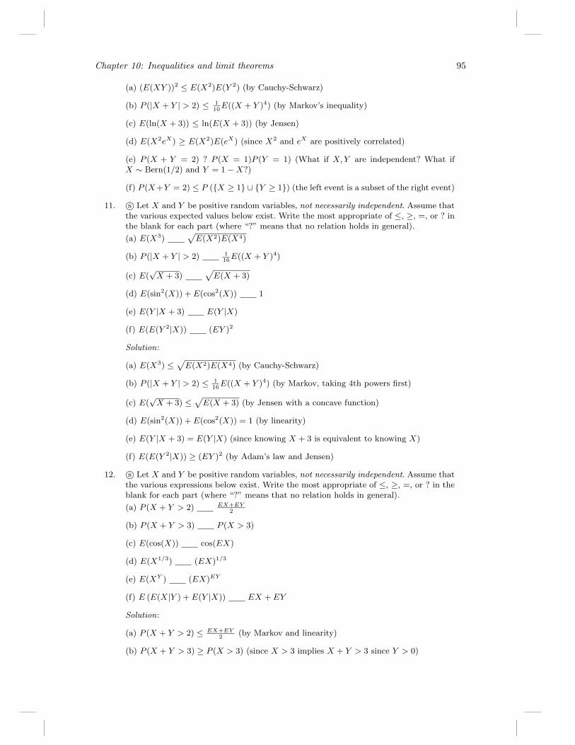
Chapter 10: Inequalities and limit theorems 95
(a) (E(XY ))2 ≤ E(X2)E(Y 2) (by Cauchy-Schwarz)
(b) P (|X + Y | > 2) ≤ 110E((X + Y )4) (by Markov’s inequality)
(c) E(ln(X + 3)) ≤ ln(E(X + 3)) (by Jensen)
(d) E(X2eX) ≥ E(X2)E(eX) (since X2 and eX are positively correlated)
(e) P (X + Y = 2) ? P (X = 1)P (Y = 1) (What if X,Y are independent? What ifX ∼ Bern(1/2) and Y = 1−X?)
(f) P (X+Y = 2) ≤ P ({X ≥ 1} ∪ {Y ≥ 1}) (the left event is a subset of the right event)
11. s© Let X and Y be positive random variables, not necessarily independent. Assume thatthe various expected values below exist. Write the most appropriate of ≤, ≥, =, or ? inthe blank for each part (where “?” means that no relation holds in general).
(a) E(X3)√E(X2)E(X4)
(b) P (|X + Y | > 2) 116E((X + Y )4)
(c) E(√X + 3)
√E(X + 3)
(d) E(sin2(X)) + E(cos2(X)) 1
(e) E(Y |X + 3) E(Y |X)
(f) E(E(Y 2|X)) (EY )2
Solution:
(a) E(X3) ≤√E(X2)E(X4) (by Cauchy-Schwarz)
(b) P (|X + Y | > 2) ≤ 116E((X + Y )4) (by Markov, taking 4th powers first)
(c) E(√X + 3) ≤
√E(X + 3) (by Jensen with a concave function)
(d) E(sin2(X)) + E(cos2(X)) = 1 (by linearity)
(e) E(Y |X + 3) = E(Y |X) (since knowing X + 3 is equivalent to knowing X)
(f) E(E(Y 2|X)) ≥ (EY )2 (by Adam’s law and Jensen)
12. s© Let X and Y be positive random variables, not necessarily independent. Assume thatthe various expressions below exist. Write the most appropriate of ≤, ≥, =, or ? in theblank for each part (where “?” means that no relation holds in general).
(a) P (X + Y > 2) EX+EY2
(b) P (X + Y > 3) P (X > 3)
(c) E(cos(X)) cos(EX)
(d) E(X1/3) (EX)1/3
(e) E(XY ) (EX)EY
(f) E (E(X|Y ) + E(Y |X)) EX + EY
Solution:
(a) P (X + Y > 2) ≤ EX+EY2
(by Markov and linearity)
(b) P (X + Y > 3) ≥ P (X > 3) (since X > 3 implies X + Y > 3 since Y > 0)
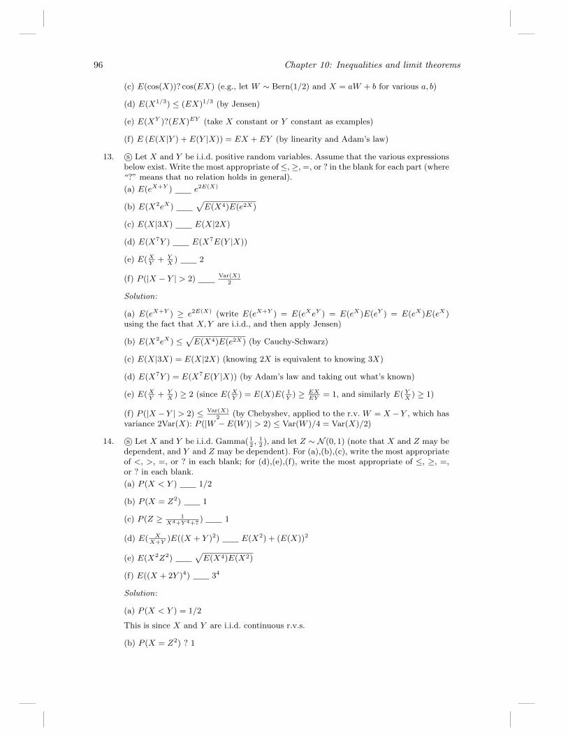
96 Chapter 10: Inequalities and limit theorems
(c) E(cos(X))? cos(EX) (e.g., let W ∼ Bern(1/2) and X = aW + b for various a, b)
(d) E(X1/3) ≤ (EX)1/3 (by Jensen)
(e) E(XY )?(EX)EY (take X constant or Y constant as examples)
(f) E (E(X|Y ) + E(Y |X)) = EX + EY (by linearity and Adam’s law)
13. s© Let X and Y be i.i.d. positive random variables. Assume that the various expressionsbelow exist. Write the most appropriate of ≤, ≥, =, or ? in the blank for each part (where“?” means that no relation holds in general).
(a) E(eX+Y ) e2E(X)
(b) E(X2eX)√E(X4)E(e2X)
(c) E(X|3X) E(X|2X)
(d) E(X7Y ) E(X7E(Y |X))
(e) E(XY
+ YX
) 2
(f) P (|X − Y | > 2) Var(X)2
Solution:
(a) E(eX+Y ) ≥ e2E(X) (write E(eX+Y ) = E(eXeY ) = E(eX)E(eY ) = E(eX)E(eX)using the fact that X,Y are i.i.d., and then apply Jensen)
(b) E(X2eX) ≤√E(X4)E(e2X) (by Cauchy-Schwarz)
(c) E(X|3X) = E(X|2X) (knowing 2X is equivalent to knowing 3X)
(d) E(X7Y ) = E(X7E(Y |X)) (by Adam’s law and taking out what’s known)
(e) E(XY
+ YX
) ≥ 2 (since E(XY
) = E(X)E( 1Y
) ≥ EXEY
= 1, and similarly E( YX
) ≥ 1)
(f) P (|X −Y | > 2) ≤ Var(X)2
(by Chebyshev, applied to the r.v. W = X −Y , which hasvariance 2Var(X): P (|W − E(W )| > 2) ≤ Var(W )/4 = Var(X)/2)
14. s© Let X and Y be i.i.d. Gamma( 12, 12), and let Z ∼ N (0, 1) (note that X and Z may be
dependent, and Y and Z may be dependent). For (a),(b),(c), write the most appropriateof <, >, =, or ? in each blank; for (d),(e),(f), write the most appropriate of ≤, ≥, =,or ? in each blank.
(a) P (X < Y ) 1/2
(b) P (X = Z2) 1
(c) P (Z ≥ 1X4+Y 4+7
) 1
(d) E( XX+Y
)E((X + Y )2) E(X2) + (E(X))2
(e) E(X2Z2)√E(X4)E(X2)
(f) E((X + 2Y )4) 34
Solution:
(a) P (X < Y ) = 1/2
This is since X and Y are i.i.d. continuous r.v.s.
(b) P (X = Z2) ? 1
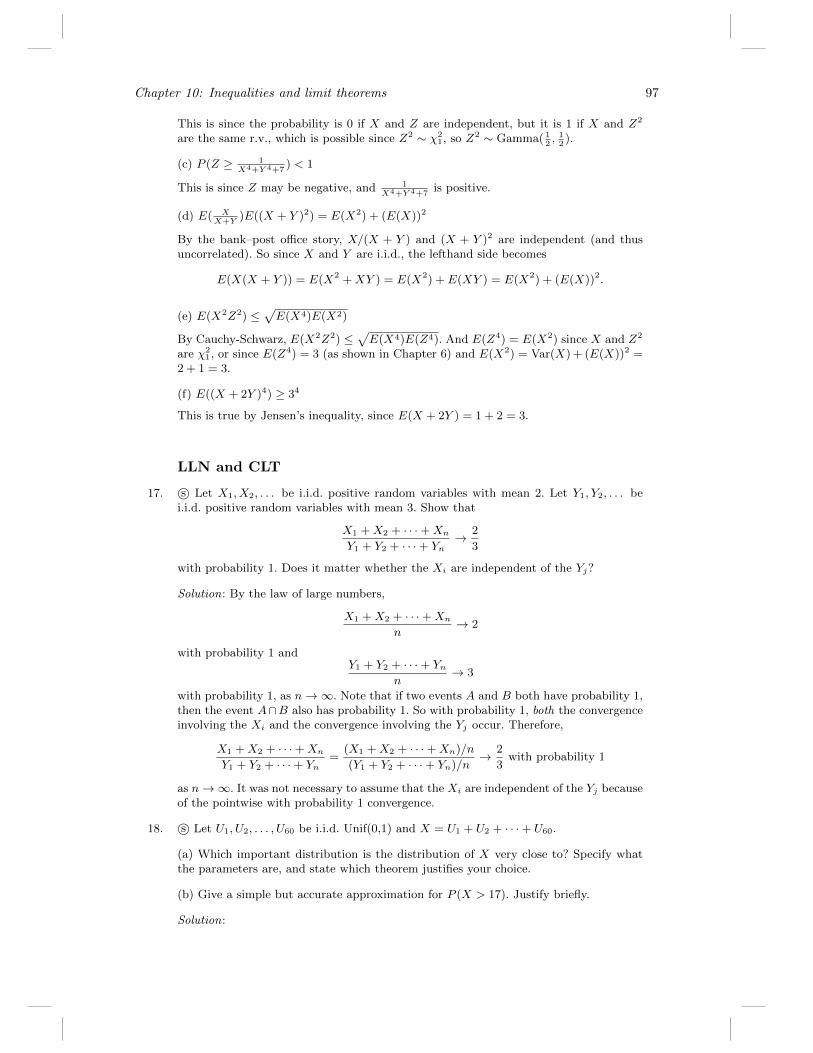
Chapter 10: Inequalities and limit theorems 97
This is since the probability is 0 if X and Z are independent, but it is 1 if X and Z2
are the same r.v., which is possible since Z2 ∼ χ21, so Z2 ∼ Gamma( 1
2, 12).
(c) P (Z ≥ 1X4+Y 4+7
) < 1
This is since Z may be negative, and 1X4+Y 4+7
is positive.
(d) E( XX+Y
)E((X + Y )2) = E(X2) + (E(X))2
By the bank–post office story, X/(X + Y ) and (X + Y )2 are independent (and thusuncorrelated). So since X and Y are i.i.d., the lefthand side becomes
E(X(X + Y )) = E(X2 +XY ) = E(X2) + E(XY ) = E(X2) + (E(X))2.
(e) E(X2Z2) ≤√E(X4)E(X2)
By Cauchy-Schwarz, E(X2Z2) ≤√E(X4)E(Z4). And E(Z4) = E(X2) since X and Z2
are χ21, or since E(Z4) = 3 (as shown in Chapter 6) and E(X2) = Var(X) + (E(X))2 =
2 + 1 = 3.
(f) E((X + 2Y )4) ≥ 34
This is true by Jensen’s inequality, since E(X + 2Y ) = 1 + 2 = 3.
LLN and CLT
17. s© Let X1, X2, . . . be i.i.d. positive random variables with mean 2. Let Y1, Y2, . . . bei.i.d. positive random variables with mean 3. Show that
X1 +X2 + · · ·+XnY1 + Y2 + · · ·+ Yn
→ 2
3
with probability 1. Does it matter whether the Xi are independent of the Yj?
Solution: By the law of large numbers,
X1 +X2 + · · ·+Xnn
→ 2
with probability 1 andY1 + Y2 + · · ·+ Yn
n→ 3
with probability 1, as n→∞. Note that if two events A and B both have probability 1,then the event A∩B also has probability 1. So with probability 1, both the convergenceinvolving the Xi and the convergence involving the Yj occur. Therefore,
X1 +X2 + · · ·+XnY1 + Y2 + · · ·+ Yn
=(X1 +X2 + · · ·+Xn)/n
(Y1 + Y2 + · · ·+ Yn)/n→ 2
3with probability 1
as n→∞. It was not necessary to assume that the Xi are independent of the Yj becauseof the pointwise with probability 1 convergence.
18. s© Let U1, U2, . . . , U60 be i.i.d. Unif(0,1) and X = U1 + U2 + · · ·+ U60.
(a) Which important distribution is the distribution of X very close to? Specify whatthe parameters are, and state which theorem justifies your choice.
(b) Give a simple but accurate approximation for P (X > 17). Justify briefly.
Solution:
98 Chapter 10: Inequalities and limit theorems
(a) By the central limit theorem, the distribution is approximately N (30, 5) sinceE(X) = 30,Var(X) = 60/12 = 5.
(b) We have
P (X > 17) = 1− P (X ≤ 17) = 1− P(X − 30√
5≤ −13√
5
)≈ 1−Φ
(−13√
5
)= Φ
(13√
5
).
Since 13/√
5 > 5, and we already have Φ(3) ≈ 0.9985 by the 68-95-99.7% rule, the valueis extremely close to 1.
19. s© Let Vn ∼ χ2n and Tn ∼ tn for all positive integers n.
(a) Find numbers an and bn such that an(Vn− bn) converges in distribution to N (0, 1).
(b) Show that T 2n/(n+ T 2
n) has a Beta distribution (without using calculus).
Solution:
(a) By definition of χ2n, we can take Vn = Z2
1 + · · · + Z2n, where Zj ∼ N (0, 1) inde-
pendently. We have E(Z21 ) = 1 and E(Z4
1 ) = 3, so Var(Z21 ) = 2. By the CLT, if we
standardize Vn it will go to N (0, 1):
Z21 + · · ·+ Z2
n − n√2n
→ N (0, 1) in distribution.
So we can take an = 1√2n
, bn = n.
(b) We can take Tn = Z0/√Vn/n, with Z0 ∼ N (0, 1) independent of Vn. Then we have
T 2n/(n+T 2
n) = Z20/(Z
20 +Vn), with Z2
0 ∼ Gamma(1/2, 1/2), Vn ∼ Gamma(n/2, 1/2). Bythe bank–post office story, Z2
0/(Z20 + Vn) ∼ Beta(1/2, n/2).
20. s© Let T1, T2, . . . be i.i.d. Student-t r.v.s with m ≥ 3 degrees of freedom. Find constantsan and bn (in terms of m and n) such that an(T1 + T2 + · · · + Tn − bn) converges toN (0, 1) in distribution as n→∞.
Solution: First let us find the mean and variance of each Tj . Let T = Z√V/m
with
Z ∼ N (0, 1) independent of V ∼ χ2m. By LOTUS, for G ∼ Gamma(a, λ), E(Gr) is
λ−rΓ(a+ r)/Γ(a) for r > −a, and does not exist for r ≤ −a. So
E(T ) = E(Z)E(1√V/m
) = 0,
Var(T ) = E(T 2)− (ET )2 = mE(Z2)E
(1
V
)= m
(1/2)Γ(m/2− 1)
Γ(m/2)
=mΓ(m/2− 1)
2Γ(m/2)
=m/2
m/2− 1=
m
m− 2.
By the CLT, this is true for
bn = E(T1) + . . .+ E(Tn) = 0,
an =1√
Var(T1) + · · ·+ Var(Tn)=
√m− 2
mn.

Chapter 10: Inequalities and limit theorems 99
21. s© (a) Let Y = eX , with X ∼ Expo(3). Find the mean and variance of Y .
(b) For Y1, . . . , Yn i.i.d. with the same distribution as Y from (a), what is the approxi-mate distribution of the sample mean Yn = 1
n
∑nj=1 Yj when n is large?
Solution:
(a) By LOTUS,
E(Y ) =
∫ ∞0
ex(3e−3x)dx =3
2,
E(Y 2) =
∫ ∞0
e2x(3e−3x)dx = 3.
So E(Y ) = 3/2,Var(Y ) = 3− 9/4 = 3/4.
(b) By the CLT, Yn is approximately N ( 32, 34n
) for large n.
22. s© (a) Explain why the Pois(n) distribution is approximately Normal if n is a largepositive integer (specifying what the parameters of the Normal are).
(b) Stirling’s formula is an amazingly accurate approximation for factorials:
n! ≈√
2πn(ne
)n,
where in fact the ratio of the two sides goes to 1 as n → ∞. Use (a) to give aquick heuristic derivation of Stirling’s formula by using a Normal approximation tothe probability that a Pois(n) r.v. is n, with the continuity correction: first writeP (N = n) = P (n− 1
2< N < n+ 1
2), where N ∼ Pois(n).
Solution:
(a) Let Sn = X1 + · · · + Xn, with X1, X2, . . . i.i.d. ∼ Pois(1). Then Sn ∼ Pois(n) andfor n large, Sn is approximately N (n, n) by the CLT.
(b) Let N ∼ Pois(n) and X ∼ N (n, n). Then
P (N = n) ≈ P(n− 1
2< X < n+
1
2
)=
1√2πn
∫ n+1/2
n−1/2
e−(x−n)2
2n dx.
The integral is approximately 1 since the interval of integration has length 1 and forlarge n the integrand is very close to 1 throughout the interval. So
e−nnn/n! ≈ (2πn)−1/2.
Rearranging this gives exactly Stirling’s formula.
23. s© (a) Consider i.i.d. Pois(λ) r.v.s X1, X2, . . . . The MGF of Xj is M(t) = eλ(et−1). Find
the MGF Mn(t) of the sample mean Xn = 1n
∑nj=1Xj .
(b) Find the limit of Mn(t) as n → ∞. (You can do this with almost no calculationusing a relevant theorem; or you can use (a) and the fact that ex ≈ 1 + x if x is verysmall.)
Solution:
(a) The MGF is
E(etn(X1+···+Xn)) =
(E(e
tnX1))n
= enλ(et/n−1),
since the Xj are i.i.d. and E(etnX1) is the MGF of X1 evaluated at t/n.
(b) By the law of large numbers, Xn → λ with probability 1. The MGF of the constantλ (viewed as an r.v. that always equals λ) is etλ. Thus, Mn(t)→ etλ as n→∞.
100 Chapter 10: Inequalities and limit theorems
Mixed practice
31. s© Let X and Y be independent standard Normal r.v.s and let R2 = X2 + Y 2 (whereR > 0 is the distance from (X,Y ) to the origin).
(a) The distribution of R2 is an example of three of the important distributions wehave seen. State which three of these distributions R2 is an instance of, specifying theparameter values.
(b) Find the PDF of R.
Hint: Start with the PDF fW (w) of W = R2.
(c) Find P (X > 2Y + 3) in terms of the standard Normal CDF Φ.
(d) Compute Cov(R2, X). Are R2 and X independent?
Solution:
(a) It is χ22, Expo(1/2), and Gamma(1,1/2).
(b) Since R =√W with fW (w) = 1
2e−w/2, we have
fR(r) = fW (w)|dw/dr| = 1
2e−w/22r = re−r
2/2, for r > 0.
(This is the Rayleigh distribution, which was seen in Example 5.1.7.)
(c) We have
P (X > 2Y + 3) = P (X − 2Y > 3) = 1− Φ
(3√5
)since X − 2Y ∼ N (0, 5).
(d) They are not independent since knowing X gives information about R2, e.g., X2
being large implies that R2 is large. But R2 and X are uncorrelated:
Cov(R2, X) = Cov(X2+Y 2, X) = Cov(X2, X)+Cov(Y 2, X) = E(X3)−(EX2)(EX)+0 = 0.
32. s© Let Z1, . . . , Zn ∼ N (0, 1) be i.i.d.
(a) As a function of Z1, create an Expo(1) r.v. X (your answer can also involve thestandard Normal CDF Φ).
(b) Let Y = e−R, where R =√Z2
1 + · · ·+ Z2n. Write down (but do not evaluate) an
integral for E(Y ).
(c) Let X1 = 3Z1 − 2Z2 and X2 = 4Z1 + 6Z2. Determine whether X1 and X2 areindependent (be sure to mention which results you’re using).
Solution:
(a) Use Z1 to get a Uniform and then the Uniform to get X: we have Φ(Z1) ∼ Unif(0, 1),and we can then take X = − log(1−Φ(Z1)). By symmetry, we can also use − log(Φ(Z1)).
Sanity check : 0 < Φ(Z1) < 1, so − ln(Φ(Z1)) is well-defined and positive.
(b) Let W = Z21 + · · · + Z2
n ∼ χ2n, so Y = e−
√W . We will use LOTUS to write E(Y )
using the PDF of W (there are other possible ways to use LOTUS here, but this issimplest since we get a single integral and we know the χ2
n PDF). This gives
E(Y ) =
∫ ∞0
e−√w 1
2n/2Γ(n/2)wn/2−1e−w/2dw.
(c) They are uncorrelated:
Cov(X1, X2) = 12Var(Z1) + 10Cov(Z1, Z2)− 12Var(Z2) = 0.
Chapter 10: Inequalities and limit theorems 101
Also, (X1, X2) is Multivariate Normal since any linear combination of X1, X2 can bewritten as a linear combination of Z1, Z2 (and thus is Normal since the sum of twoindependent Normals is Normal). So X1 and X2 are independent.
33. s© Let X1, X2, . . . be i.i.d. positive r.v.s. with mean µ, and let Wn = X1X1+···+Xn
.
(a) Find E(Wn).
Hint: Consider X1X1+···+Xn
+ X2X1+···+Xn
+ · · ·+ XnX1+···+Xn
.
(b) What random variable does nWn converge to (with probability 1) as n→∞?
(c) For the case that Xj ∼ Expo(λ), find the distribution of Wn, preferably withoutusing calculus. (If it is one of the named distributions, state its name and specify theparameters; otherwise, give the PDF.)
Solution:
(a) The expression in the hint equals 1, and by linearity and symmetry its expectedvalue is nE(Wn). So E(Wn) = 1/n.
Sanity check : in the case that the Xj are actually constants, X1X1+···+Xn
reduces to 1n
.Also in the case Xj ∼ Expo(λ), Part (c) shows that the answer should reduce to themean of a Beta(1, n− 1) (which is 1
n).
(b) By LLN, with probability 1 we have
nWn =X1
(X1 + · · ·+Xn)/n→ X1
µas n→∞.
Sanity check : the answer should be a random variable since it’s asked what randomvariable nWn converges to. It should not depend on n since we let n→∞.
(c) Recall that X1 ∼ Gamma(1) and X2 + · · ·+Xn ∼ Gamma(n−1). By the connectionbetween Beta and Gamma (i.e., the bank–post office story), Wn ∼ Beta(1, n− 1).
Sanity check : The r.v. Wn clearly always takes values between 0 and 1, and the meanshould agree with the answer from (a).

Chapter 11: Markov chains
Markov property
1. s© Let X0, X1, X2, . . . be a Markov chain. Show that X0, X2, X4, X6, . . . is also a Markovchain, and explain why this makes sense intuitively.
Solution: Let Yn = X2n; we need to show Y0, Y1, . . . is a Markov chain. By the def-inition of a Markov chain, we know that X2n+1, X2n+2, . . . (“the future” if we definethe “present” to be time 2n) is conditionally independent of X0, X1, . . . , X2n−2, X2n−1
(“the past”), given X2n. So given Yn, we have that Yn+1, Yn+2, . . . is conditionally in-dependent of Y0, Y1, . . . , Yn−1. Thus,
P (Yn+1 = y|Y0 = y0, . . . , Yn = yn) = P (Yn+1 = y|Yn = yn).
2. s© Let X0, X1, X2, . . . be an irreducible Markov chain with state space {1, 2, . . . ,M},M ≥ 3, transition matrix Q = (qij), and stationary distribution s = (s1, . . . , sM ). Letthe initial state X0 follow the stationary distribution, i.e., P (X0 = i) = si.
(a) On average, how many of X0, X1, . . . , X9 equal 3? (In terms of s; simplify.)
(b) Let Yn = (Xn−1)(Xn−2). For M = 3, find an example of Q (the transition matrixfor the original chain X0, X1, . . . ) where Y0, Y1, . . . is Markov, and another example ofQ where Y0, Y1, . . . is not Markov. In your examples, make qii > 0 for at least one i andmake sure it is possible to get from any state to any other state eventually.
Solution:
(a) Since X0 has the stationary distribution, all of X0, X1, . . . have the stationary dis-tribution. By indicator random variables, the expected value is 10s3.
(b) Note that Yn is 0 if Xn is 1 or 2, and Yn is 2 otherwise. So the Yn process can be
viewed as merging states 1 and 2 of the Xn-chain into one state. Knowing the history ofYn’s means knowing when the Xn-chain is in state 3, without being able to distinguishstate 1 from state 2.
If q13 = q23, then Yn is Markov since given Yn, even knowing the past X0, . . . , Xn doesnot affect the transition probabilities. But if q13 6= q23, then the Yn past history cangive useful information about Xn, affecting the transition probabilities. So one example(not the only possible example!) is
Q1 =
13
13
13
13
13
13
13
13
13
(Markov) Q2 =
12
12
013
13
13
1 0 0
(not Markov).
(c) The stationary distribution is uniform over all states:
s = (1/M, 1/M, . . . , 1/M).
This is because(1/M 1/M . . . 1/M
)Q =
1
M
(1 1 . . . 1
)Q =
(1/M 1/M . . . 1/M
),
where the matrix multiplication was done by noting that multiplying a row vector of1’s times Q gives the column sums of Q.
103
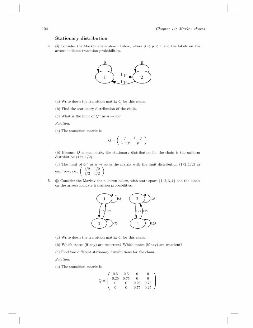
104 Chapter 11: Markov chains
Stationary distribution
4. s© Consider the Markov chain shown below, where 0 < p < 1 and the labels on thearrows indicate transition probabilities.
1
p
21-p1-p
p
(a) Write down the transition matrix Q for this chain.
(b) Find the stationary distribution of the chain.
(c) What is the limit of Qn as n→∞?
Solution:
(a) The transition matrix is
Q =
(p 1− p
1− p p
)
(b) Because Q is symmetric, the stationary distribution for the chain is the uniformdistribution (1/2, 1/2).
(c) The limit of Qn as n → ∞ is the matrix with the limit distribution (1/2, 1/2) as
each row, i.e.,
(1/2 1/21/2 1/2
).
5. s© Consider the Markov chain shown below, with state space {1, 2, 3, 4} and the labelson the arrows indicate transition probabilities.
1 0.5
2
0.5 0.25
0.75
3 0.25
4
0.75 0.75
0.25
(a) Write down the transition matrix Q for this chain.
(b) Which states (if any) are recurrent? Which states (if any) are transient?
(c) Find two different stationary distributions for the chain.
Solution:
(a) The transition matrix is
Q =
0.5 0.5 0 00.25 0.75 0 0
0 0 0.25 0.750 0 0.75 0.25
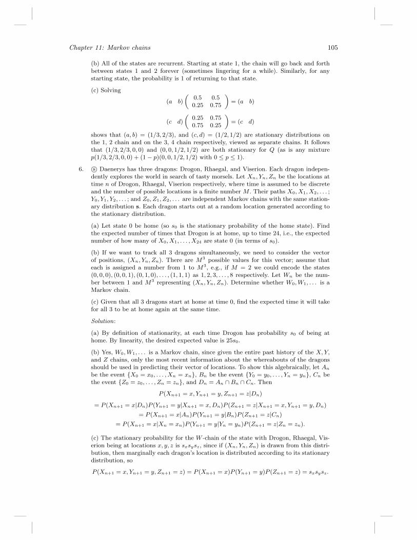
Chapter 11: Markov chains 105
(b) All of the states are recurrent. Starting at state 1, the chain will go back and forthbetween states 1 and 2 forever (sometimes lingering for a while). Similarly, for anystarting state, the probability is 1 of returning to that state.
(c) Solving
(a b)
(0.5 0.50.25 0.75
)= (a b)
(c d)
(0.25 0.750.75 0.25
)= (c d)
shows that (a, b) = (1/3, 2/3), and (c, d) = (1/2, 1/2) are stationary distributions onthe 1, 2 chain and on the 3, 4 chain respectively, viewed as separate chains. It followsthat (1/3, 2/3, 0, 0) and (0, 0, 1/2, 1/2) are both stationary for Q (as is any mixturep(1/3, 2/3, 0, 0) + (1− p)(0, 0, 1/2, 1/2) with 0 ≤ p ≤ 1).
6. s© Daenerys has three dragons: Drogon, Rhaegal, and Viserion. Each dragon indepen-dently explores the world in search of tasty morsels. Let Xn, Yn, Zn be the locations attime n of Drogon, Rhaegal, Viserion respectively, where time is assumed to be discreteand the number of possible locations is a finite number M . Their paths X0, X1, X2, . . . ;Y0, Y1, Y2, . . . ; and Z0, Z1, Z2, . . . are independent Markov chains with the same station-ary distribution s. Each dragon starts out at a random location generated according tothe stationary distribution.
(a) Let state 0 be home (so s0 is the stationary probability of the home state). Findthe expected number of times that Drogon is at home, up to time 24, i.e., the expectednumber of how many of X0, X1, . . . , X24 are state 0 (in terms of s0).
(b) If we want to track all 3 dragons simultaneously, we need to consider the vectorof positions, (Xn, Yn, Zn). There are M3 possible values for this vector; assume thateach is assigned a number from 1 to M3, e.g., if M = 2 we could encode the states(0, 0, 0), (0, 0, 1), (0, 1, 0), . . . , (1, 1, 1) as 1, 2, 3, . . . , 8 respectively. Let Wn be the num-ber between 1 and M3 representing (Xn, Yn, Zn). Determine whether W0,W1, . . . is aMarkov chain.
(c) Given that all 3 dragons start at home at time 0, find the expected time it will takefor all 3 to be at home again at the same time.
Solution:
(a) By definition of stationarity, at each time Drogon has probability s0 of being athome. By linearity, the desired expected value is 25s0.
(b) Yes, W0,W1, . . . is a Markov chain, since given the entire past history of the X,Y,and Z chains, only the most recent information about the whereabouts of the dragonsshould be used in predicting their vector of locations. To show this algebraically, let Anbe the event {X0 = x0, . . . , Xn = xn}, Bn be the event {Y0 = y0, . . . , Yn = yn}, Cn bethe event {Z0 = z0, . . . , Zn = zn}, and Dn = An ∩Bn ∩ Cn. Then
P (Xn+1 = x, Yn+1 = y, Zn+1 = z|Dn)
= P (Xn+1 = x|Dn)P (Yn+1 = y|Xn+1 = x,Dn)P (Zn+1 = z|Xn+1 = x, Yn+1 = y,Dn)
= P (Xn+1 = x|An)P (Yn+1 = y|Bn)P (Zn+1 = z|Cn)
= P (Xn+1 = x|Xn = xn)P (Yn+1 = y|Yn = yn)P (Zn+1 = z|Zn = zn).
(c) The stationary probability for the W -chain of the state with Drogon, Rhaegal, Vis-erion being at locations x, y, z is sxsysz, since if (Xn, Yn, Zn) is drawn from this distri-bution, then marginally each dragon’s location is distributed according to its stationarydistribution, so
P (Xn+1 = x, Yn+1 = y, Zn+1 = z) = P (Xn+1 = x)P (Yn+1 = y)P (Zn+1 = z) = sxsysz.
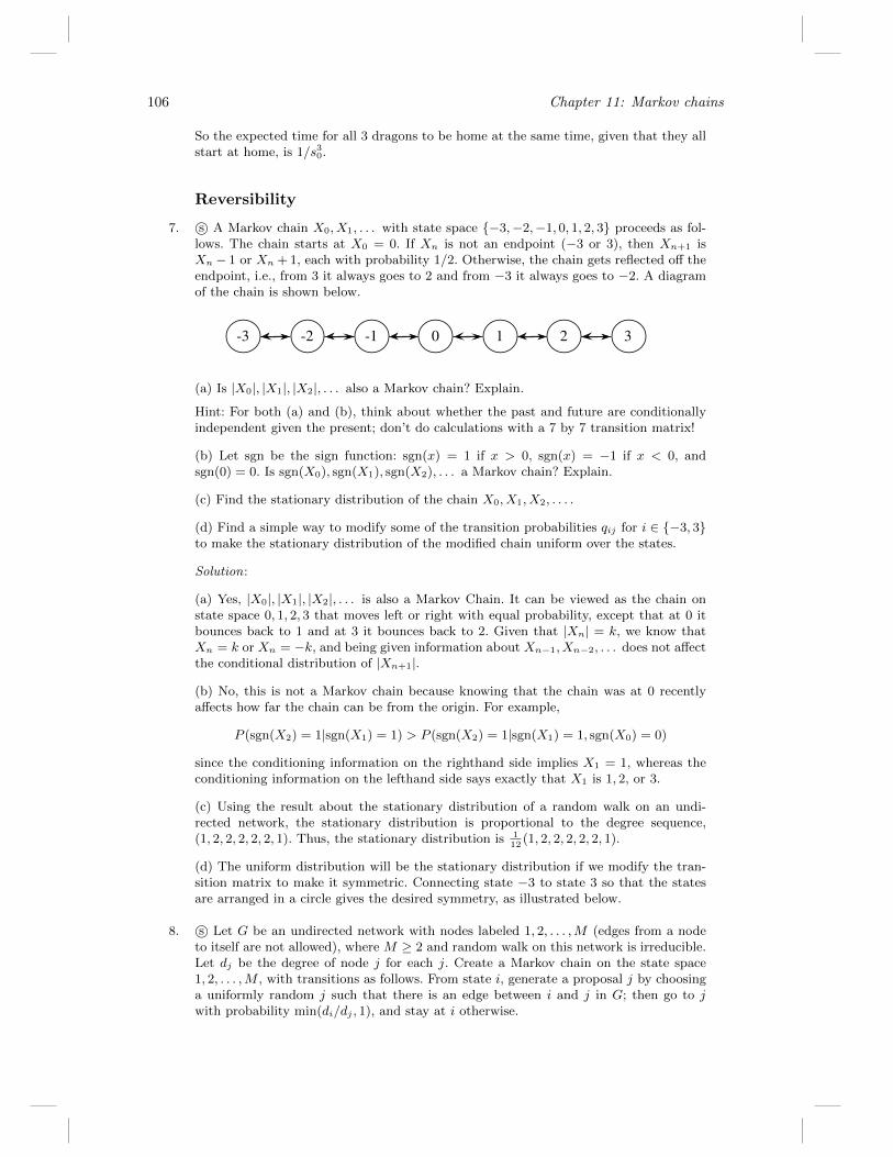
106 Chapter 11: Markov chains
So the expected time for all 3 dragons to be home at the same time, given that they allstart at home, is 1/s30.
Reversibility
7. s© A Markov chain X0, X1, . . . with state space {−3,−2,−1, 0, 1, 2, 3} proceeds as fol-lows. The chain starts at X0 = 0. If Xn is not an endpoint (−3 or 3), then Xn+1 isXn − 1 or Xn + 1, each with probability 1/2. Otherwise, the chain gets reflected off theendpoint, i.e., from 3 it always goes to 2 and from −3 it always goes to −2. A diagramof the chain is shown below.
-3 -2 -1 0 1 2 3
(a) Is |X0|, |X1|, |X2|, . . . also a Markov chain? Explain.
Hint: For both (a) and (b), think about whether the past and future are conditionallyindependent given the present; don’t do calculations with a 7 by 7 transition matrix!
(b) Let sgn be the sign function: sgn(x) = 1 if x > 0, sgn(x) = −1 if x < 0, andsgn(0) = 0. Is sgn(X0), sgn(X1), sgn(X2), . . . a Markov chain? Explain.
(c) Find the stationary distribution of the chain X0, X1, X2, . . . .
(d) Find a simple way to modify some of the transition probabilities qij for i ∈ {−3, 3}to make the stationary distribution of the modified chain uniform over the states.
Solution:
(a) Yes, |X0|, |X1|, |X2|, . . . is also a Markov Chain. It can be viewed as the chain onstate space 0, 1, 2, 3 that moves left or right with equal probability, except that at 0 itbounces back to 1 and at 3 it bounces back to 2. Given that |Xn| = k, we know thatXn = k or Xn = −k, and being given information about Xn−1, Xn−2, . . . does not affectthe conditional distribution of |Xn+1|.
(b) No, this is not a Markov chain because knowing that the chain was at 0 recentlyaffects how far the chain can be from the origin. For example,
P (sgn(X2) = 1|sgn(X1) = 1) > P (sgn(X2) = 1|sgn(X1) = 1, sgn(X0) = 0)
since the conditioning information on the righthand side implies X1 = 1, whereas theconditioning information on the lefthand side says exactly that X1 is 1, 2, or 3.
(c) Using the result about the stationary distribution of a random walk on an undi-rected network, the stationary distribution is proportional to the degree sequence,(1, 2, 2, 2, 2, 2, 1). Thus, the stationary distribution is 1
12(1, 2, 2, 2, 2, 2, 1).
(d) The uniform distribution will be the stationary distribution if we modify the tran-sition matrix to make it symmetric. Connecting state −3 to state 3 so that the statesare arranged in a circle gives the desired symmetry, as illustrated below.
8. s© Let G be an undirected network with nodes labeled 1, 2, . . . ,M (edges from a nodeto itself are not allowed), where M ≥ 2 and random walk on this network is irreducible.Let dj be the degree of node j for each j. Create a Markov chain on the state space1, 2, . . . ,M , with transitions as follows. From state i, generate a proposal j by choosinga uniformly random j such that there is an edge between i and j in G; then go to jwith probability min(di/dj , 1), and stay at i otherwise.
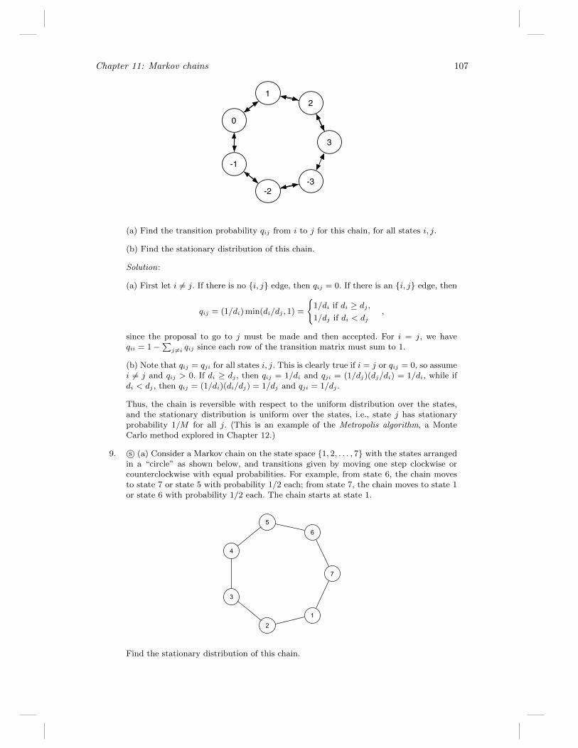
Chapter 11: Markov chains 107
-3-2
-1
0
12
3
(a) Find the transition probability qij from i to j for this chain, for all states i, j.
(b) Find the stationary distribution of this chain.
Solution:
(a) First let i 6= j. If there is no {i, j} edge, then qij = 0. If there is an {i, j} edge, then
qij = (1/di) min(di/dj , 1) =
{1/di if di ≥ dj ,1/dj if di < dj
,
since the proposal to go to j must be made and then accepted. For i = j, we haveqii = 1−
∑j 6=i qij since each row of the transition matrix must sum to 1.
(b) Note that qij = qji for all states i, j. This is clearly true if i = j or qij = 0, so assumei 6= j and qij > 0. If di ≥ dj , then qij = 1/di and qji = (1/dj)(dj/di) = 1/di, while ifdi < dj , then qij = (1/di)(di/dj) = 1/dj and qji = 1/dj .
Thus, the chain is reversible with respect to the uniform distribution over the states,and the stationary distribution is uniform over the states, i.e., state j has stationaryprobability 1/M for all j. (This is an example of the Metropolis algorithm, a MonteCarlo method explored in Chapter 12.)
9. s© (a) Consider a Markov chain on the state space {1, 2, . . . , 7} with the states arrangedin a “circle” as shown below, and transitions given by moving one step clockwise orcounterclockwise with equal probabilities. For example, from state 6, the chain movesto state 7 or state 5 with probability 1/2 each; from state 7, the chain moves to state 1or state 6 with probability 1/2 each. The chain starts at state 1.
1
2
3
4
5
6
7
Find the stationary distribution of this chain.
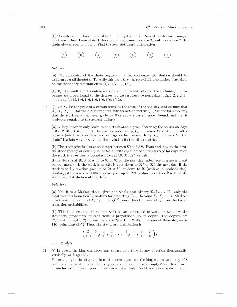
108 Chapter 11: Markov chains
(b) Consider a new chain obtained by “unfolding the circle”. Now the states are arrangedas shown below. From state 1 the chain always goes to state 2, and from state 7 thechain always goes to state 6. Find the new stationary distribution.
1 2 3 4 5 6 7
Solution:
(a) The symmetry of the chain suggests that the stationary distribution should beuniform over all the states. To verify this, note that the reversibility condition is satisfied.So the stationary distribution is (1/7, 1/7, . . . , 1/7).
(b) By the result about random walk on an undirected network, the stationary proba-bilities are proportional to the degrees. So we just need to normalize (1, 2, 2, 2, 2, 2, 1),obtaining (1/12, 1/6, 1/6, 1/6, 1/6, 1/6, 1/12).
10. s© Let Xn be the price of a certain stock at the start of the nth day, and assume thatX0, X1, X2, . . . follows a Markov chain with transition matrix Q. (Assume for simplicitythat the stock price can never go below 0 or above a certain upper bound, and that itis always rounded to the nearest dollar.)
(a) A lazy investor only looks at the stock once a year, observing the values on days0, 365, 2 · 365, 3 · 365, . . . . So the investor observes Y0, Y1, . . . , where Yn is the price aftern years (which is 365n days; you can ignore leap years). Is Y0, Y1, . . . also a Markovchain? Explain why or why not; if so, what is its transition matrix?
(b) The stock price is always an integer between $0 and $28. From each day to the next,the stock goes up or down by $1 or $2, all with equal probabilities (except for days whenthe stock is at or near a boundary, i.e., at $0, $1, $27, or $28).
If the stock is at $0, it goes up to $1 or $2 on the next day (after receiving governmentbailout money). If the stock is at $28, it goes down to $27 or $26 the next day. If thestock is at $1, it either goes up to $2 or $3, or down to $0 (with equal probabilities);similarly, if the stock is at $27 it either goes up to $28, or down to $26 or $25. Find thestationary distribution of the chain.
Solution:
(a) Yes, it is a Markov chain: given the whole past history Y0, Y1, . . . , Yn, only themost recent information Yn matters for predicting Yn+1, because X0, X1, . . . is Markov.The transition matrix of Y0, Y1, . . . is Q365, since the kth power of Q gives the k-steptransition probabilities.
(b) This is an example of random walk on an undirected network, so we know thestationary probability of each node is proportional to its degree. The degrees are(2, 3, 4, 4, . . . , 4, 4, 3, 2), where there are 29 − 4 = 25 4’s. The sum of these degrees is110 (coincidentally?). Thus, the stationary distribution is(
2
110,
3
110,
4
110,
4
110, . . . ,
4
110,
4
110,
3
110,
2
110
),
with 25 4110
’s.
11. s© In chess, the king can move one square at a time in any direction (horizontally,vertically, or diagonally).
For example, in the diagram, from the current position the king can move to any of 8possible squares. A king is wandering around on an otherwise empty 8× 8 chessboard,where for each move all possibilities are equally likely. Find the stationary distribution
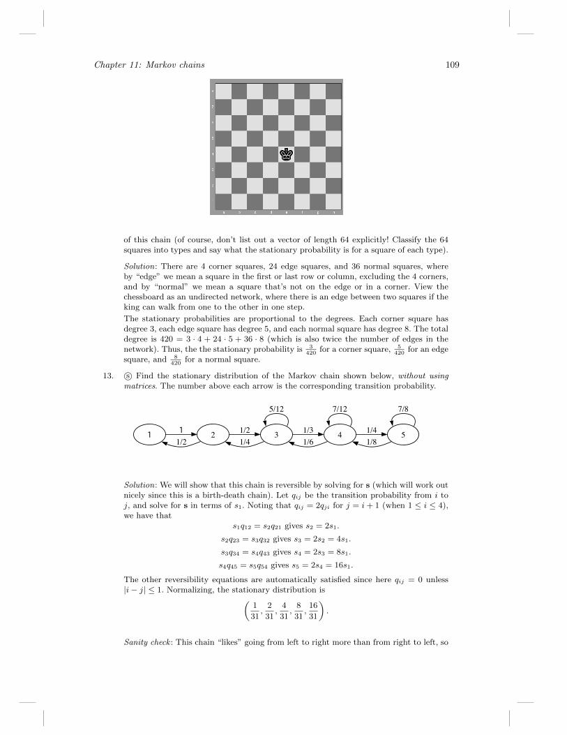
Chapter 11: Markov chains 109
of this chain (of course, don’t list out a vector of length 64 explicitly! Classify the 64squares into types and say what the stationary probability is for a square of each type).
Solution: There are 4 corner squares, 24 edge squares, and 36 normal squares, whereby “edge” we mean a square in the first or last row or column, excluding the 4 corners,and by “normal” we mean a square that’s not on the edge or in a corner. View thechessboard as an undirected network, where there is an edge between two squares if theking can walk from one to the other in one step.
The stationary probabilities are proportional to the degrees. Each corner square hasdegree 3, each edge square has degree 5, and each normal square has degree 8. The totaldegree is 420 = 3 · 4 + 24 · 5 + 36 · 8 (which is also twice the number of edges in thenetwork). Thus, the the stationary probability is 3
420for a corner square, 5
420for an edge
square, and 8420
for a normal square.
13. s© Find the stationary distribution of the Markov chain shown below, without usingmatrices. The number above each arrow is the corresponding transition probability.
1 211/2
31/21/4
5/12
41/31/6
7/12
51/41/8
7/8
Solution: We will show that this chain is reversible by solving for s (which will work outnicely since this is a birth-death chain). Let qij be the transition probability from i toj, and solve for s in terms of s1. Noting that qij = 2qji for j = i+ 1 (when 1 ≤ i ≤ 4),we have that
s1q12 = s2q21 gives s2 = 2s1.
s2q23 = s3q32 gives s3 = 2s2 = 4s1.
s3q34 = s4q43 gives s4 = 2s3 = 8s1.
s4q45 = s5q54 gives s5 = 2s4 = 16s1.
The other reversibility equations are automatically satisfied since here qij = 0 unless|i− j| ≤ 1. Normalizing, the stationary distribution is(
1
31,
2
31,
4
31,
8
31,
16
31
).
Sanity check : This chain “likes” going from left to right more than from right to left, so
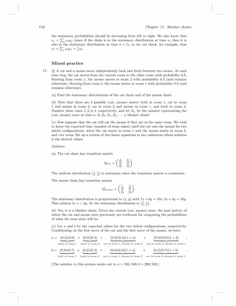
110 Chapter 11: Markov chains
the stationary probabilities should be increasing from left to right. We also know thatsj =
∑i siqij (since if the chain is in the stationary distribution at time n, then it is
also in the stationary distribution at time n + 1), so we can check, for example, thats1 =
∑i siqi1 = 1
2s2.
Mixed practice
17. s© A cat and a mouse move independently back and forth between two rooms. At eachtime step, the cat moves from the current room to the other room with probability 0.8.Starting from room 1, the mouse moves to room 2 with probability 0.3 (and remainsotherwise). Starting from room 2, the mouse moves to room 1 with probability 0.6 (andremains otherwise).
(a) Find the stationary distributions of the cat chain and of the mouse chain.
(b) Note that there are 4 possible (cat, mouse) states: both in room 1, cat in room1 and mouse in room 2, cat in room 2 and mouse in room 1, and both in room 2.Number these cases 1, 2, 3, 4, respectively, and let Zn be the number representing the(cat, mouse) state at time n. Is Z0, Z1, Z2, . . . a Markov chain?
(c) Now suppose that the cat will eat the mouse if they are in the same room. We wishto know the expected time (number of steps taken) until the cat eats the mouse for twoinitial configurations: when the cat starts in room 1 and the mouse starts in room 2,and vice versa. Set up a system of two linear equations in two unknowns whose solutionis the desired values.
Solution:
(a) The cat chain has transition matrix
Qcat =
(210
810
810
210
).
The uniform distribution ( 12, 12) is stationary since the transition matrix is symmetric.
The mouse chain has transition matrix
Qmouse =
(710
310
610
410
).
The stationary distribution is proportional to (x, y) with 7x+ 6y = 10x, 3x+ 4y = 10y.This reduces to x = 2y. So the stationary distribution is ( 2
3, 13).
(b) Yes, it is a Markov chain. Given the current (cat, mouse) state, the past history ofwhere the cat and mouse were previously are irrelevant for computing the probabilitiesof what the next state will be.
(c) Let a and b be the expected values for the two initial configurations, respectively.Conditioning on the first move of the cat and the first move of the mouse, we have
a = (0.2)(0.6)︸ ︷︷ ︸both in room 1
+ (0.8)(0.4)︸ ︷︷ ︸both in room 2
+ (0.2)(0.4)(1 + a)︸ ︷︷ ︸cat in room 1, mouse in room 2
+ (0.8)(0.6)(1 + b)︸ ︷︷ ︸cat in room 2, mouse in room 1
,
b = (0.8)(0.7)︸ ︷︷ ︸both in room 1
+ (0.2)(0.3)︸ ︷︷ ︸both in room 2
+ (0.8)(0.3)(1 + a)︸ ︷︷ ︸cat in room 1, mouse in room 2
+ (0.2)(0.7)(1 + b)︸ ︷︷ ︸cat in room 2, mouse in room 1
.
(The solution to this system works out to a = 335/169, b = 290/169.)