Solutions to some exercises from Bayesian Data Analysis,second edition, by Gelman, Carlin, Stern, and Rubin

4 Mar 2012These solutions are in progress. For more information on either the solutions or the book (pub-

lished by CRC), check the website, http://www.stat.columbia.edu/∼gelman/book/

For each graph and some other computations, we include the code used to create it using the Scomputer language. The S commands are set off from the text and appear in typewriter font.

If you find any mistakes, please notify us by e-mailing to gelman@stat.columbia.edu. Thankyou very much.

c©1996, 1997, 2000, 2001, 2003, 2004, 2006, 2007, 2009, 2010 Andrew Gelman, John Carlin, HalStern, and Rich Charnigo. We also thank Jiangtao Du for help in preparing some of these solutionsand Ewan Cameron, Rob Creecy, Xin Feng, Lei Guo, Yi Lu, Pejman Mohammadi, Fei Shi, KenWilliams, Corey Yanovsky, and Peng Yu for finding mistakes.

We have complete (or essentially complete) solutions for the following exercises:Chapter 1: 1, 2, 3, 4, 5, 6Chapter 2: 1, 2, 3, 4, 5, 7, 8, 9, 10, 11, 12, 13, 16, 18, 19, 22Chapter 3: 1, 2, 3, 5, 9, 10Chapter 4: 2, 3, 4Chapter 5: 1, 2, 3, 5, 6, 7, 8, 9, 10Chapter 6: 1, 5, 6, 7Chapter 7: 1, 2, 7, 15Chapter 8: 1, 2, 4, 6, 8Chapter 11: 1, 2Chapter 12: 6, 7Chapter 14: 1, 3, 4, 7Chapter 17: 1

1.1a.

p(y) = Pr(θ = 1)p(y|θ = 1) + Pr(θ = 2)p(y|θ = 2)

= 0.5N(y|1, 22) + 0.5N(y|2, 22).

y-5 0 5 10

y <- seq(-7,10,.02)

dens <- 0.5*dnorm(y,1,2) + 0.5*dnorm(y,2,2)

plot (y, dens, ylim=c(0,1.1*max(dens)),

type="l", xlab="y", ylab="", xaxs="i",

yaxs="i", yaxt="n", bty="n", cex=2)

1.1b.

Pr(θ = 1|y = 1) =p(θ = 1& y = 1)

p(θ = 1& y = 1) + p(θ = 2& y = 1)

=Pr(θ = 1)p(y = 1|θ = 1)

Pr(θ = 1)p(y = 1|θ = 1) + Pr(θ = 2)p(y = 1|θ = 2)

=0.5N(1|1, 22)

0.5N(1|1, 22) + 0.5N(1|2, 22)= 0.53.

1

1.1c. As σ → ∞, the posterior density for θ approaches the prior (the data contain no information):Pr(θ = 1|y = 1) → 1

2 . As σ → 0, the posterior density for θ becomes concentrated at 1: Pr(θ =1|y = 1) → 1.

1.2. (1.7): For each component ui, the univariate result (1.6) states that E(ui) = E(E(ui|v)); thus,E(u) = E(E(u|v)), componentwise.

(1.8): For diagonal elements of var(u), the univariate result (1.8) states that var(ui) = E(var(ui|v))+var(E(ui|v)). For off-diagonal elements,

E[cov(ui, uj|v)] + cov[E(ui|v),E(uj |v)]= E[E(uiuj |v)− E(ui|v)E(uj |v)] + E[E(ui|v)E(uj |v)]− E[E(ui|v)]E[E(uj |v)]= E(uiuj)− E[E(ui|v)E(uj|v)] + E[E(ui|v)E(uj |v)]− E[E(ui|v)]E[E(uj |v)]= E(uiuj)− E(ui)E(uj) = cov(ui, uj).

1.3. Note: We will use “Xx” to indicate all heterozygotes (written as “Xx or xX” in the Exercise).

Pr(child is Xx | child has brown eyes& parents have brown eyes)

=0 · (1− p)4 + 1

2 · 4p(1− p)3 + 12 · 4p2(1− p)2

1 · (1− p)4 + 1 · 4p(1− p)3 + 34 · 4p2(1− p)2

=2p(1− p) + 2p2

(1 − p)2 + 4p(1− p) + 3p2

=2p

1 + 2p.

To figure out the probability that Judy is a heterozygote, use the above posterior probability asa prior probability for a new calculation that includes the additional information that her n childrenare brown-eyed (with the father Xx):

Pr(Judy is Xx |n children all have brown eyes& all previous information) =

2p1+2p ·

(34

)n

2p1+2p ·

(34

)n+ 1

1+2p · 1.

Given that Judy’s children are all brown-eyed, her grandchild has blue eyes only if Judy’s childis Xx. We compute this probability, recalling that we know the child is brown-eyed and we knowJudy’s spouse is a heterozygote:

Pr(Judy’s child is Xx | all the given information)

= Pr((Judy is Xx&Judy’s child is Xx) or (Judy is XX&Judy’s child is Xx) | all the given information)

=

2p1+2p ·

(34

)n

2p1+2p ·

(34

)n+ 1

1+2p

(2

3

)

+

11+2p

2p1+2p ·

(34

)n+ 1

1+2p

(1

2

)

.

Given that Judy’s child is Xx, the probability of the grandchild having blue eyes is 0, 1/4, or 1/2,if Judy’s child’s spouse is XX, Xx, or xx, respectively. Given random mating, these events haveprobability (1− p)2, 2p(1− p), and p2, respectively, and so

Pr(Grandchild is xx | all the given information)

=

23

2p1+2p ·

(34

)n+ 1

21

1+2p

2p1+2p ·

(34

)n+ 1

1+2p

(1

42p(1− p) +

1

2p2)

=

23

2p1+2p ·

(34

)n+ 1

21

1+2p

2p1+2p ·

(34

)n+ 1

1+2p

(1

2p

)

.

2

1.4a. Use relative frequencies: Pr(A|B) = # of cases of A and B# of cases of B

.

Pr(favorite wins | point spread=8) =8

12= 0.67

Pr(favorite wins by at least 8 | point spread=8) =5

12= 0.42

Pr(favorite wins by at least 8 | point spread=8& favorite wins) =5

8= 0.63.

1.4b. Use the normal approximation for d = (score differential− point spread): d ∼ N(0, 13.862).Note: “favorite wins” means “score differential > 0”; “favorite wins by at least 8” means “scoredifferential ≥ 8.”

Pr(favorite wins | point spread=8) = Φ

(8.5

13.86

)

= 0.730

Pr(favorite wins by at least 8 | point spread=8) = Φ

(0.5

13.86

)

= 0.514

Pr(favorite wins by at least 8 | point spread=8& favorite wins) =0.514

0.730= 0.70.

Note: the values of 0.5 and 8.5 in the above calculations are corrections for the discreteness ofscores (the score differential must be an integer). The notation Φ is used for the normal cumulativedistribution function.

1.5a. There are many possible answers to this question. One possibility goes as follows. We knowthat most Congressional elections are contested by two candidates, and that each candidate typicallyreceives between 30% and 70% of the vote. For a given Congressional election, let n be the totalnumber of votes cast and y be the number received by the candidate from the Democratic party. Ifwe assume (as a first approximation, and with no specific knowledge of this election), that y/n isuniformly distributed between 30% and 70%, then

Pr(election is tied|n) = Pr(y = n/2) =

{1

0.4n if n is even0 if n is odd

.

If we assume that n is about 200,000, with a 1/2 chance of being even, then this approximationgives Pr(election is tied) ≈ 1

160,000 .A national election has 435 individual elections, and so the probability of at least one of them

being tied, in this analysis, is (assuming independence, since we have no specific knowledge aboutthe elections),

Pr(at least one election is tied) = 1−(

1− 1

160,000

)435

≈ 435

160,000≈ 1/370.

A common mistake here is to assume an overly-precise model such as y ∼ Bin(n, 1/2). As in thefootball point spreads example, it is important to estimate probabilities based on observed outcomesrather than constructing them from a theoretical model. This is relevant even in an example such asthis one, where almost no information is available. (In this example, using a binomial model impliesthat almost all elections are extremely close, which is not true in reality.)

1.5b. An empirical estimate of the probability that an election will be decided within 100 votes is49/20,597. The event that an election is tied is (y = n/2) or, equivalently, |2y−n| = 0; and the eventthat an election is decided within 100 votes is |y−(n−y)| ≤ 100 or, equivalently, |2y−n| ≤ 100. Now,

3

(2y−n) is a random variable that can take on integer values. Given that n is so large (at least 50,000),and that each voter votes without knowing the outcome of the election, it seems that the distributionof (2y−n) should be nearly exactly uniform near 0. Then Pr(|2y−n| = 0) = 1

201 Pr(|2y−n| ≤ 100),and we estimate the probability that an election is tied as 1

20149

20,597 . As in 1.5a, the probability that

any of 435 elections will be tied is then approximately 435 1201

4920,597 ≈ 1/190.

(We did not make use of the fact that 6 elections were decided by fewer than 10 votes, becauseit seems reasonable to assume a uniform distribution over the scale of 100 votes, on which moreinformation is available.)

1.6. First determine the unconditional probabilities:

Pr(identical twins& twin brother) = Pr(identical twins) Pr(both boys | identical twins) = 1

2· 1

300

Pr(fraternal twins& twin brother) = Pr(fraternal twins) Pr(both boys | fraternal twins) = 1

4· 1

125.

The conditional probability that Elvis was an identical twin is

Pr(identical twins | twin brother) =Pr(identical twins& twin brother)

Pr(twin brother)

=12 · 1

30012 · 1

300 + 14 · 1

125

=5

11.

2.1. Prior density:p(θ) ∝ θ3(1− θ)3.

Likelihood:

Pr(data|θ) =

(10

0

)

(1 − θ)10 +

(10

1

)

θ(1 − θ)9 +

(10

2

)

θ2(1− θ)8

= (1− θ)10 + 10θ(1− θ)9 + 45θ2(1− θ)8.

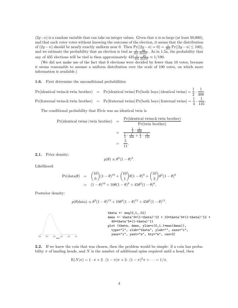
Posterior density:

p(θ|data) ∝ θ3(1 − θ)13 + 10θ4(1− θ)12 + 45θ5(1− θ)11.

theta0.0 0.2 0.4 0.6 0.8 1.0

theta <- seq(0,1,.01)

dens <- theta^3*(1-theta)^13 + 10*theta^4*(1-theta)^12 +

45*theta^5*(1-theta)^11

plot (theta, dens, ylim=c(0,1.1*max(dens)),

type="l", xlab="theta", ylab="", xaxs="i",

yaxs="i", yaxt="n", bty="n", cex=2)

2.2. If we knew the coin that was chosen, then the problem would be simple: if a coin has proba-bility π of landing heads, and N is the number of additional spins required until a head, then

E(N |π) = 1 · π + 2 · (1− π)π + 3 · (1− π)2π + · · · = 1/π.

4

Let TT denote the event that the first two spins are tails, and let C be the coin that was chosen.By Bayes’ rule,

Pr(C = C1|TT ) =Pr(C = C1) Pr(TT |C = C1)

Pr(C = C1) Pr(TT |C = C1) + Pr(C = C2) Pr(TT |C = C2)

=0.5(0.4)2

0.5(0.4)2 + 0.5(0.6)2=

16

52.

The posterior expectation of N is then

E(N |TT ) = E[E(N |TT,C)|TT ]= Pr(C = C1|TT )E(N |C = C1, TT ) + Pr(C = C2|TT )E(N |C = C2, TT )

=16

52

1

0.6+

36

52

1

0.4= 2.24.

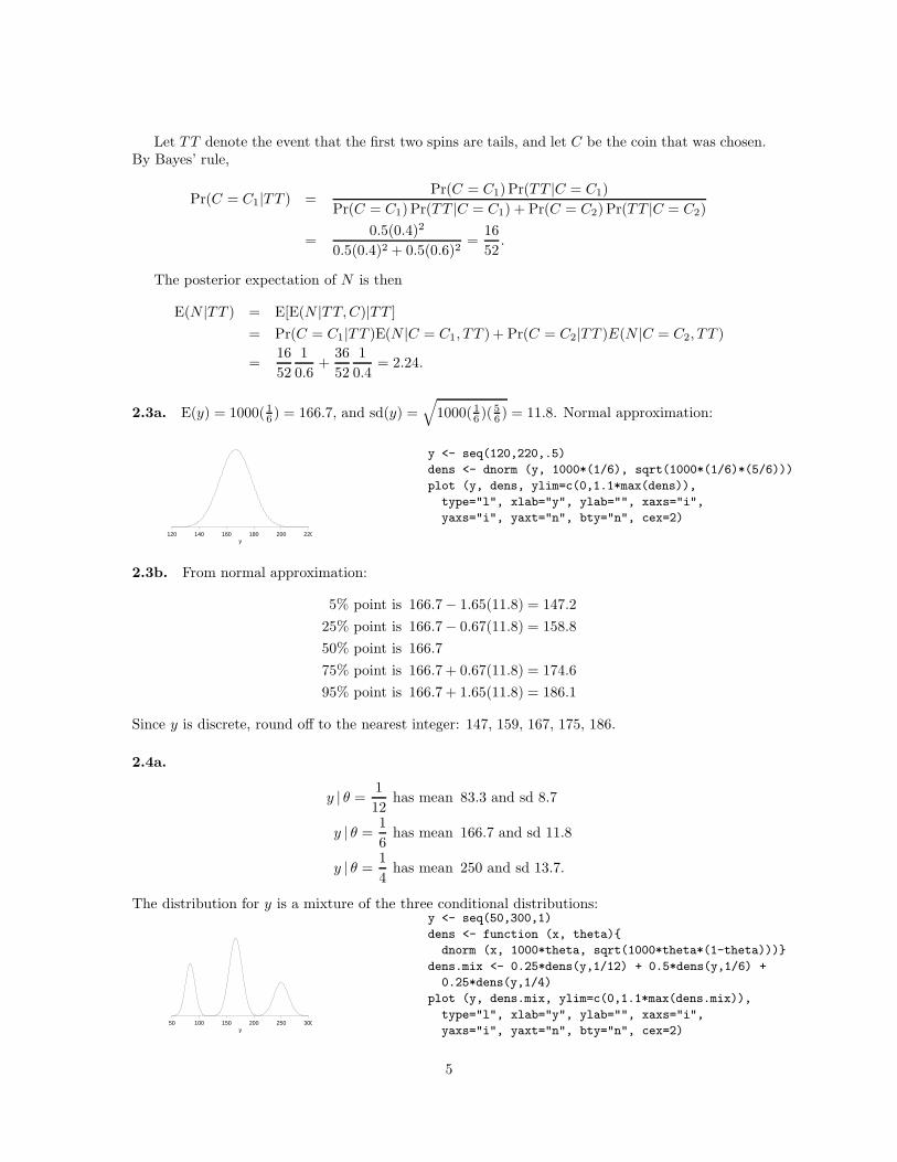
2.3a. E(y) = 1000(16 ) = 166.7, and sd(y) =√

1000(16 )(56 ) = 11.8. Normal approximation:

y120 140 160 180 200 220

y <- seq(120,220,.5)

dens <- dnorm (y, 1000*(1/6), sqrt(1000*(1/6)*(5/6)))

plot (y, dens, ylim=c(0,1.1*max(dens)),

type="l", xlab="y", ylab="", xaxs="i",

yaxs="i", yaxt="n", bty="n", cex=2)

2.3b. From normal approximation:

5% point is 166.7− 1.65(11.8) = 147.2

25% point is 166.7− 0.67(11.8) = 158.8

50% point is 166.7

75% point is 166.7 + 0.67(11.8) = 174.6

95% point is 166.7 + 1.65(11.8) = 186.1

Since y is discrete, round off to the nearest integer: 147, 159, 167, 175, 186.

2.4a.

y | θ =1

12has mean 83.3 and sd 8.7

y | θ =1

6has mean 166.7 and sd 11.8

y | θ =1

4has mean 250 and sd 13.7.

The distribution for y is a mixture of the three conditional distributions:

y50 100 150 200 250 300

y <- seq(50,300,1)

dens <- function (x, theta){

dnorm (x, 1000*theta, sqrt(1000*theta*(1-theta)))}

dens.mix <- 0.25*dens(y,1/12) + 0.5*dens(y,1/6) +

0.25*dens(y,1/4)

plot (y, dens.mix, ylim=c(0,1.1*max(dens.mix)),

type="l", xlab="y", ylab="", xaxs="i",

yaxs="i", yaxt="n", bty="n", cex=2)

5

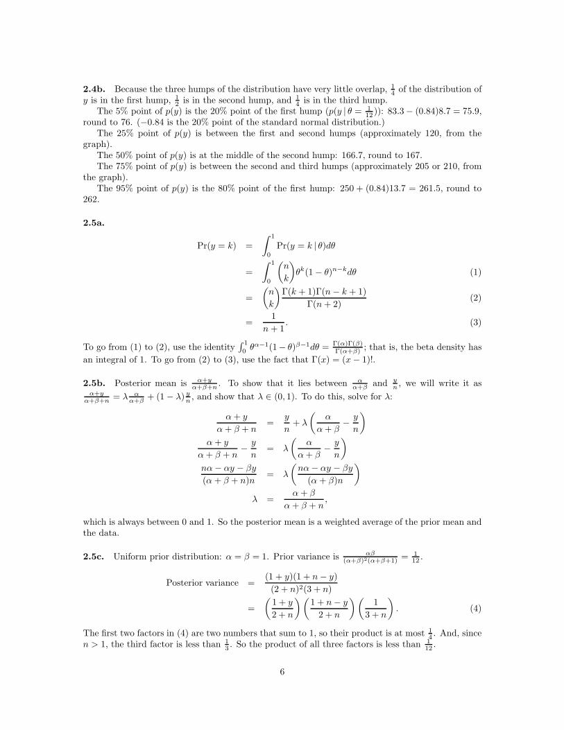
2.4b. Because the three humps of the distribution have very little overlap, 14 of the distribution of

y is in the first hump, 12 is in the second hump, and 1

4 is in the third hump.The 5% point of p(y) is the 20% point of the first hump (p(y | θ = 1

12 )): 83.3− (0.84)8.7 = 75.9,round to 76. (−0.84 is the 20% point of the standard normal distribution.)

The 25% point of p(y) is between the first and second humps (approximately 120, from thegraph).

The 50% point of p(y) is at the middle of the second hump: 166.7, round to 167.The 75% point of p(y) is between the second and third humps (approximately 205 or 210, from

the graph).The 95% point of p(y) is the 80% point of the first hump: 250 + (0.84)13.7 = 261.5, round to

262.

2.5a.

Pr(y = k) =

∫ 1

0

Pr(y = k | θ)dθ

=

∫ 1

0

(n

k

)

θk(1− θ)n−kdθ (1)

=

(n

k

)Γ(k + 1)Γ(n− k + 1)

Γ(n+ 2)(2)

=1

n+ 1. (3)

To go from (1) to (2), use the identity∫ 1

0 θα−1(1− θ)β−1dθ = Γ(α)Γ(β)Γ(α+β) ; that is, the beta density has

an integral of 1. To go from (2) to (3), use the fact that Γ(x) = (x− 1)!.

2.5b. Posterior mean is α+yα+β+n . To show that it lies between α

α+β and yn , we will write it as

α+yα+β+n = λ α

α+β + (1− λ) yn , and show that λ ∈ (0, 1). To do this, solve for λ:

α+ y

α+ β + n=

y

n+ λ

(α

α+ β− y

n

)

α+ y

α+ β + n− y

n= λ

(α

α+ β− y

n

)

nα− αy − βy

(α + β + n)n= λ

(nα− αy − βy

(α + β)n

)

λ =α+ β

α+ β + n,

which is always between 0 and 1. So the posterior mean is a weighted average of the prior mean andthe data.

2.5c. Uniform prior distribution: α = β = 1. Prior variance is αβ(α+β)2(α+β+1) =

112 .

Posterior variance =(1 + y)(1 + n− y)

(2 + n)2(3 + n)

=

(1 + y

2 + n

)(1 + n− y

2 + n

)(1

3 + n

)

. (4)

The first two factors in (4) are two numbers that sum to 1, so their product is at most 14 . And, since

n > 1, the third factor is less than 13 . So the product of all three factors is less than 1

12 .

6

2.5d. There is an infinity of possible correct solutions to this exercise. For large n, the posteriorvariance is definitely lower, so if this is going to happen, it will be for small n. Try n = 1 and y = 1(1 success in 1 try). Playing around with low values of α and β, we find: if α = 1, β = 5, then priorvariance is 0.0198, and posterior variance is 0.0255.

2.7a. The binomial can be put in the form of an exponential family with (using the notation of thelast part of Section 2.4) f(y) =

(ny

), g(θ) = (1−θ)n, u(y) = y and natural parameter φ(θ) = log( θ

1−θ ).

A uniform prior density on φ(θ), p(φ) ∝ 1 on the entire real line, can be transformed to give theprior density for θ = eφ/(1 + eφ):

q(θ) = p

(eφ

1 + eφ

) ∣∣∣∣

d

dθlog

(θ

1− θ

)∣∣∣∣∝ θ−1(1− θ)−1.

2.7b. If y = 0 then p(θ|y) ∝ θ−1(1− θ)n−1 which has infinite integral over any interval near θ = 0.Similarly for y = n at θ = 1.

2.8a.

θ|y ∼ N

( 1402 180 +

n202 150

1402 + n

202

,1

1402 + n

202

)

2.8b.

y|y ∼ N

( 1402 180 +

n202 150

1402 + n

202

,1

1402 + n

202

+ 202)

2.8c.

95% posterior interval for θ | y = 150, n = 10: 150.7± 1.96(6.25) = [138, 163]

95% posterior interval for y | y = 150, n = 10: 150.7± 1.96(20.95) = [110, 192]

2.8d.

95% posterior interval for θ | y = 150, n = 100: [146, 154]

95% posterior interval for y | y = 150, n = 100: [111, 189]

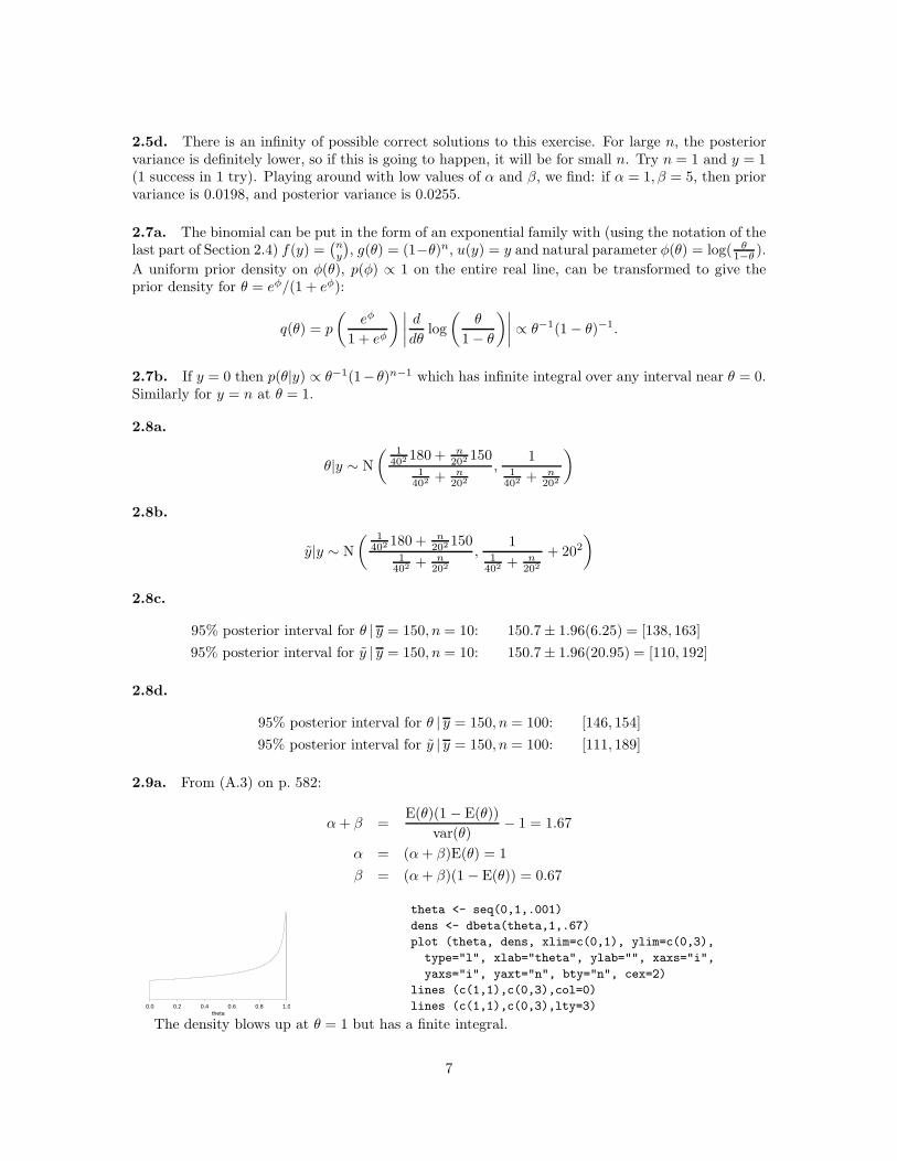
2.9a. From (A.3) on p. 582:

α+ β =E(θ)(1 − E(θ))

var(θ)− 1 = 1.67

α = (α+ β)E(θ) = 1

β = (α+ β)(1 − E(θ)) = 0.67

theta0.0 0.2 0.4 0.6 0.8 1.0

theta <- seq(0,1,.001)

dens <- dbeta(theta,1,.67)

plot (theta, dens, xlim=c(0,1), ylim=c(0,3),

type="l", xlab="theta", ylab="", xaxs="i",

yaxs="i", yaxt="n", bty="n", cex=2)

lines (c(1,1),c(0,3),col=0)

lines (c(1,1),c(0,3),lty=3)

The density blows up at θ = 1 but has a finite integral.

7

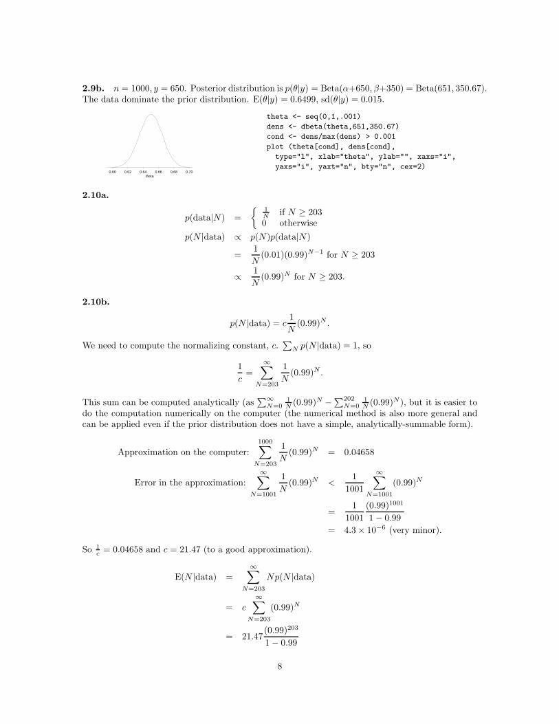
2.9b. n = 1000, y = 650. Posterior distribution is p(θ|y) = Beta(α+650, β+350) = Beta(651, 350.67).The data dominate the prior distribution. E(θ|y) = 0.6499, sd(θ|y) = 0.015.

theta0.60 0.62 0.64 0.66 0.68 0.70

theta <- seq(0,1,.001)

dens <- dbeta(theta,651,350.67)

cond <- dens/max(dens) > 0.001

plot (theta[cond], dens[cond],

type="l", xlab="theta", ylab="", xaxs="i",

yaxs="i", yaxt="n", bty="n", cex=2)

2.10a.

p(data|N) =

{1N if N ≥ 2030 otherwise

p(N |data) ∝ p(N)p(data|N)

=1

N(0.01)(0.99)N−1 for N ≥ 203

∝ 1

N(0.99)N for N ≥ 203.

2.10b.

p(N |data) = c1

N(0.99)N .

We need to compute the normalizing constant, c.∑

N p(N |data) = 1, so

1

c=

∞∑

N=203

1

N(0.99)N .

This sum can be computed analytically (as∑∞

N=01N (0.99)N −∑202

N=01N (0.99)N ), but it is easier to

do the computation numerically on the computer (the numerical method is also more general andcan be applied even if the prior distribution does not have a simple, analytically-summable form).

Approximation on the computer:

1000∑

N=203

1

N(0.99)N = 0.04658

Error in the approximation:

∞∑

N=1001

1

N(0.99)N <

1

1001

∞∑

N=1001

(0.99)N

=1

1001

(0.99)1001

1− 0.99

= 4.3× 10−6 (very minor).

So 1c = 0.04658 and c = 21.47 (to a good approximation).

E(N |data) =∞∑

N=203

Np(N |data)

= c

∞∑

N=203

(0.99)N

= 21.47(0.99)203

1− 0.99

8

= 279.1

sd(N |data) =

√√√√

∞∑

N=203

(N − 279.1)2c1

N(0.99)N

≈

√√√√

1000∑

N=203

(N − 279.1)221.471

N(0.99)N

= 79.6.

2.10c. Many possible solutions here (see Jeffreys, 1961; Lee, 1989; and Jaynes, 1996). One ideathat does not work is the improper discrete uniform prior density on N : p(N) ∝ 1. This densityleads to an improper posterior density: p(N) ∝ 1

N , for N ≥ 203. (∑∞

N=203(1/N) = ∞.) Theprior density p(N) ∝ 1/N is improper, but leads to a proper prior density, because

∑

N 1/N2 isconvergent.

Note also that:

• If more than one data point is available (that is, if more than one cable car number is observed),then the posterior distribution is proper under all the above prior densities.

• With only one data point, perhaps it would not make much sense in practice to use a nonin-formative prior distribution here.

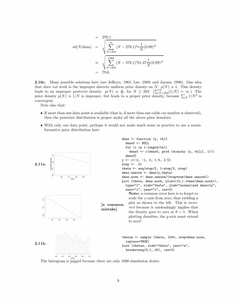
2.11a.

theta

norm

aliz

ed d

ensi

ty

0.2 0.4 0.6 0.8

0.0

0.4

0.8

1.2

dens <- function (y, th){

dens0 <- NULL

for (i in 1:length(th))

dens0 <- c(dens0, prod (dcauchy (y, th[i], 1)))

dens0}

y <- c(-2, -1, 0, 1.5, 2.5)

step <- .01

theta <- seq(step/2, 1-step/2, step)

dens.unnorm <- dens(y,theta)

dens.norm <- dens.unnorm/(step*sum(dens.unnorm))

plot (theta, dens.norm, ylim=c(0,1.1*max(dens.norm)),

type="l", xlab="theta", ylab="normalized density",

xaxs="i", yaxs="i", cex=2)

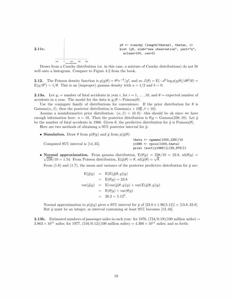
0.2 0.4 0.6 0.8

0.8

1.0

1.2

[a commonmistake]

Note: a common error here is to forget toscale the y-axis from zero, thus yielding aplot as shown to the left. This is incor-

rect because it misleadingly implies thatthe density goes to zero at θ = 1. Whenplotting densities, the y-axis must extendto zero!

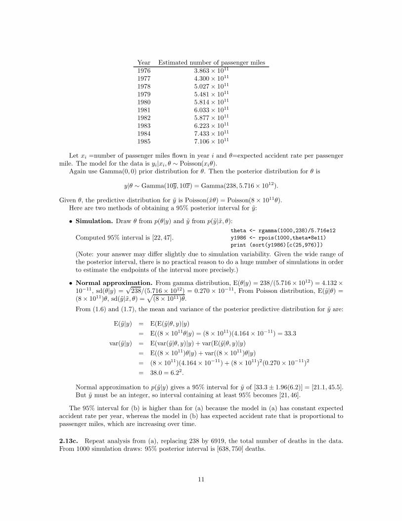
2.11b.

0.0 0.2 0.4 0.6 0.8 1.0theta

thetas <- sample (theta, 1000, step*dens.norm,

replace=TRUE)

hist (thetas, xlab="theta", yaxt="n",

breaks=seq(0,1,.05), cex=2)

The histogram is jagged because there are only 1000 simulation draws.

9

2.11c.

-200 0 200 400 600new observation

y6 <- rcauchy (length(thetas), thetas, 1)

hist (y6, xlab="new observation", yaxt="n",

nclass=100, cex=2)

Draws from a Cauchy distribution (or, in this case, a mixture of Cauchy distributions) do not fitwell onto a histogram. Compare to Figure 4.2 from the book.

2.12. The Poisson density function is p(y|θ) = θye−θ/y!, and so J(θ) = E(−d2 log p(y|θ)/dθ2|θ) =E(y/θ2) = 1/θ. This is an (improper) gamma density with a = 1/2 and b = 0.

2.13a. Let yi = number of fatal accidents in year i, for i = 1, . . . , 10, and θ = expected number ofaccidents in a year. The model for the data is yi|θ ∼ Poisson(θ).

Use the conjugate family of distributions for convenience. If the prior distribution for θ isGamma(α, β), then the posterior distribution is Gamma(α + 10y, β + 10).

Assume a noninformative prior distribution: (α, β) = (0, 0)—this should be ok since we haveenough information here: n = 10. Then the posterior distribution is θ|y ∼ Gamma(238, 10). Let ybe the number of fatal accidents in 1986. Given θ, the predictive distribution for y is Poisson(θ).

Here are two methods of obtaining a 95% posterior interval for y:

• Simulation. Draw θ from p(θ|y) and y from p(y|θ):

Computed 95% interval is [14, 35].theta <- rgamma(1000,238)/10

y1986 <- rpois(1000,theta)

print (sort(y1986)[c(25,976)])

• Normal approximation. From gamma distribution, E(θ|y) = 238/10 = 23.8, sd(θ|y) =√238/10 = 1.54. From Poisson distribution, E(y|θ) = θ, sd(y|θ) =

√θ.

From (1.6) and (1.7), the mean and variance of the posterior predictive distribution for y are:

E(y|y) = E(E(y|θ, y)|y)= E(θ|y) = 23.8

var(y|y) = E(var(y|θ, y)|y) + var(E(y|θ, y)|y)= E(θ|y) + var(θ|y)= 26.2 = 5.122.

Normal approximation to p(y|y) gives a 95% interval for y of [23.8± 1.96(5.12)] = [13.8, 33.8].But y must be an integer, so interval containing at least 95% becomes [13, 34].

2.13b. Estimated numbers of passenger miles in each year: for 1976, (734/0.19)(100 million miles) =3.863× 1011 miles; for 1977, (516/0.12)(100 million miles) = 4.300× 1011 miles; and so forth:

10

Year Estimated number of passenger miles1976 3.863× 1011

1977 4.300× 1011

1978 5.027× 1011

1979 5.481× 1011

1980 5.814× 1011

1981 6.033× 1011

1982 5.877× 1011

1983 6.223× 1011

1984 7.433× 1011

1985 7.106× 1011

Let xi =number of passenger miles flown in year i and θ=expected accident rate per passengermile. The model for the data is yi|xi, θ ∼ Poisson(xiθ).

Again use Gamma(0, 0) prior distribution for θ. Then the posterior distribution for θ is

y|θ ∼ Gamma(10y, 10x) = Gamma(238, 5.716× 1012).

Given θ, the predictive distribution for y is Poisson(xθ) = Poisson(8× 1011θ).Here are two methods of obtaining a 95% posterior interval for y:

• Simulation. Draw θ from p(θ|y) and y from p(y|x, θ):

Computed 95% interval is [22, 47].theta <- rgamma(1000,238)/5.716e12

y1986 <- rpois(1000,theta*8e11)

print (sort(y1986)[c(25,976)])

(Note: your answer may differ slightly due to simulation variability. Given the wide range ofthe posterior interval, there is no practical reason to do a huge number of simulations in orderto estimate the endpoints of the interval more precisely.)

• Normal approximation. From gamma distribution, E(θ|y) = 238/(5.716× 1012) = 4.132×10−11, sd(θ|y) =

√238/(5.716 × 1012) = 0.270 × 10−11, From Poisson distribution, E(y|θ) =

(8× 1011)θ, sd(y|x, θ) =√

(8× 1011)θ.

From (1.6) and (1.7), the mean and variance of the posterior predictive distribution for y are:

E(y|y) = E(E(y|θ, y)|y)= E((8 × 1011θ|y) = (8 × 1011)(4.164× 10−11) = 33.3

var(y|y) = E(var(y|θ, y)|y) + var(E(y|θ, y)|y)= E((8 × 1011)θ|y) + var((8× 1011)θ|y)= (8× 1011)(4.164× 10−11) + (8× 1011)2(0.270× 10−11)2

= 38.0 = 6.22.

Normal approximation to p(y|y) gives a 95% interval for y of [33.3 ± 1.96(6.2)] = [21.1, 45.5].But y must be an integer, so interval containing at least 95% becomes [21, 46].

The 95% interval for (b) is higher than for (a) because the model in (a) has constant expectedaccident rate per year, whereas the model in (b) has expected accident rate that is proportional topassenger miles, which are increasing over time.

2.13c. Repeat analysis from (a), replacing 238 by 6919, the total number of deaths in the data.From 1000 simulation draws: 95% posterior interval is [638, 750] deaths.

11

2.13d. Repeat analysis from (b), replacing 238 by 6919. From 1000 simulation draws: 95% poste-rior interval is [900, 1035] deaths.

2.13e. Just based on general knowledge, without specific reference to the data in Table 2.2, thePoisson model seems more reasonable with rate proportional to passenger miles (models (b) and(d)), because if more miles are flown in a year, you would expect more accidents. On the otherhand, if airline safety is improving, we would expect the accident rate to decline over time, so maybethe expected number of accidents would remain roughly constant (as the number of passenger milesflown is gradually increasing). The right thing to do here is to put a time trend in the model, as inExercise 3.12.

Also just based on general knowledge, we would expect accidents to be independent. But passen-ger deaths are not independent—they occur in clusters when airplanes crash. So the Poisson modelshould be more reasonable for accidents (models (a) and (b)) than for total deaths. What if youwere interested in total deaths? Then it might be reasonable to set up a compound model: a Poissondistribution for accidents, and then another distribution for deaths given accidents.

In addition, these models can be checked by comparing to data (see Exercise 6.2).

2.16a.

p(y) =

∫

p(y|θ)p(θ)dθ

=

∫ 1

0

(n

y

)

θy(1− θ)n−y Γ(α+ β)

Γ(α)Γ(β)θα−1(1 − θ)β−1dθ

=Γ(n+ 1)

Γ(y + 1)Γ(n− y + 1)

Γ(α+ β)

Γ(α)Γ(β)

∫ 1

0

θy+α−1(1− θ)n−y+β−1dθ

=Γ(n+ 1)

Γ(y + 1)Γ(n− y + 1)

Γ(α+ β)

Γ(α)Γ(β)

Γ(y + α)Γ(n− y + β)

Γ(n+ α+ β),

which is the beta-binomial density (see pp. 576–577).

2.16b. We are interested only in seeing whether p(y) varies with y, so we need only look atthe factors in p(y) that depend on y; thus, we investigate under what circumstances the quantityΓ(a+ y)Γ(b+ n− y)/Γ(y + 1)Γ(n− y + 1) changes with y.

The preceding expression evaluates to 1 if a = b = 1; hence p(y) is constant in y if a = b = 1.On the other hand, suppose that p(y) is constant in y. Then, in particular, p(0) = p(n) and

p(0) = p(1). The first equality implies that Γ(a)Γ(b+n)/Γ(1)Γ(n+1) = Γ(a+n)Γ(b)/Γ(n+1)Γ(1),so that Γ(a)Γ(b+ n) = Γ(a+ n)Γ(b).

Recalling the formula Γ(t) = (t − 1)Γ(t − 1), we must have Γ(a)Γ(b)(b + n − 1)...(b + 1)(b) =Γ(a)Γ(b)(a+n− 1)...(a+1)(a), which implies that (b+n− 1)...(b+1)(b) = (a+n− 1)...(a+1)(a).Since each term in each product is positive, it follows that a = b.

Continuing, p(0) = p(1) implies Γ(a)Γ(b + n)/Γ(1)Γ(n + 1) = Γ(a + 1)Γ(b + n − 1)/Γ(2)Γ(n);again using Γ(t) = (t−1)Γ(t−1), we have b+n−1 = na. Since a = b, this reduces to a+n−1 = na,whose only solution is a = 1.

Therefore a = b = 1 is a necessary as well as sufficient condition for p(y) to be constant in y.

2.18. Uniform prior distribution on θ means that the posterior distribution is θ|y ∼ N(17.653, 0.122/9).Then

y|y ∼ N(17.653, 0.122/9 + 0.122)

= N(17.653, 0.1262).

99% tolerance interval is [17.653± 2.58(0.126)] = [17.33, 17.98].

12

2.19a. Let u = σ2, so that σ =√u. Then p(σ2) = p(u) = p(

√u)d

√u/du = p(σ)(1/2)u−1/2 =

(1/2)p(σ)/σ, which is proportional to 1/σ2 if p(σ) ∝ σ−1.

2.19b. Proof by contradiction: The posterior density p(σ|data) is proportional to σ−1−n exp(−c/σ2),which may be written as (σ2)−1/2−n/2 exp(−c/σ2). The posterior density p(σ2|data) is proportionalto (σ2)−1−n/2 exp(−c/σ2). In the preceding expressions, we have defined c = nv/2, and we assumethis quantity to be positive.

Let (√a,√b) be the 95% interval of highest density for p(σ|data). (It can be shown using calculus

that the density function is unimodal: there is only one value of σ for which dp(σ|data)/dσ = 0.Therefore the 95% region of highest density is a single interval.) Then

a−1/2−n/2 exp(−c/a) = b−1/2−n/2 exp(−c/b).

Equivalently, (−1/2− n/2) log a− c/a = (−1/2− n/2) log b− c/b.Now, if (a, b) were the 95% interval of highest density for p(σ2|data), then

a−1−n/2 exp(−c/a) = b−1−n/2 exp(−c/b).

That is, (−1 − n/2) log a− c/a = (−1− n/2) log b− c/b. Combining the two equations, 1/2 log a =1/2 log b, so that a = b, in which case [a, b] cannot be a 95% interval, and we have a contradiction.

2.22a.

p(θ | y ≥ 100) ∝ p(y ≥ 100 | θ)p(θ)∝ exp(−100θ)θα−1 exp(−βθ)

p(θ | y ≥ 100) = Gamma(θ |α, β + 100)

The posterior mean and variance of θ are αβ+100 and α

(β+100)2 , respectively.

2.22b.

p(θ | y = 100) ∝ p(y = 100 | θ)p(θ)∝ θ exp(−100θ)θα−1 exp(−βθ)

p(θ | y = 100) = Gamma(θ |α+ 1, β + 100)

The posterior mean and variance of θ are α+1β+100 and α+1

(β+100)2 , respectively.

2.22c. Identity (2.8) says on average, the variance of θ decreases given more information: in thiscase,

E(var(θ|y) | y ≥ 100) ≤ var(θ | y ≥ 100). (5)

Plugging in y = 100 to get var(θ|y = 100) is not the same as averaging over the distribution ofy | y ≥ 100 on the left side of (5).

3.1a Label the prior distribution p(θ) as Dirichlet(a1, . . . , an). Then the posterior distributionis p(θ|y) = Dirichlet(y1 + a1, . . . , yn + an). From the properties of the Dirichlet distribution (seeAppendix A), the marginal posterior distribution of (θ1, θ2, 1− θ1 − θ2) is also Dirichlet:

p(θ1, θ2|y) ∝ θy1+a1−11 θy2+a2−1

2 (1−θ1−θ2)yrest+arest−1, where yrest = y3+. . .+yJ , arest = a3+. . .+aJ .

(This can be proved using mathematical induction, by first integrating out θn, then θn−1, and soforth, until only θ1 and θ2 remain.)

13

Now do a change of variables to (α, β) = ( θ1θ1+θ2

, θ1 + θ2). The Jacobian of this transformationis |1/β|, so the transformed density is

p(α, β|y) ∝ β(αβ)y1+a1−1((1 − α)β)y2+a2−1(1− β)yrest+arest−1

= αy1+a1−1(1− α)y2+a2−1βy1+y2+a1+a2−1(1− β)yrest+arest−1

∝ Beta(α|y1 + a1, y2 + a2)Beta(β|y1 + y2 + a1 + a2, yrest + arest).

Since the posterior density divides into separate factors for α and β, they are independent, and, asshown above, α|y ∼ Beta(y1 + a1, y2 + a2).

3.1b. The Beta(y1+a1, y2+a2) posterior distribution can also be derived from a Beta(a1, a2) priordistribution and a binomial observation y1 with sample size y1 + y2.

3.2. Assume independent uniform prior distributions on the multinomial parameters. Then theposterior distributions are independent multinomial:

(π1, π2, π3)|y ∼ Dirichlet(295, 308, 39)

(π∗1 , π

∗2 , π

∗3)|y ∼ Dirichlet(289, 333, 20),

and α1 = π1

π1+π2

, α2 =π∗

1

π∗

1+π∗

2

. From the properties of the Dirichlet distribution (see Exercise 3.1),

α1|y ∼ Beta(295, 308)

α2|y ∼ Beta(289, 333).

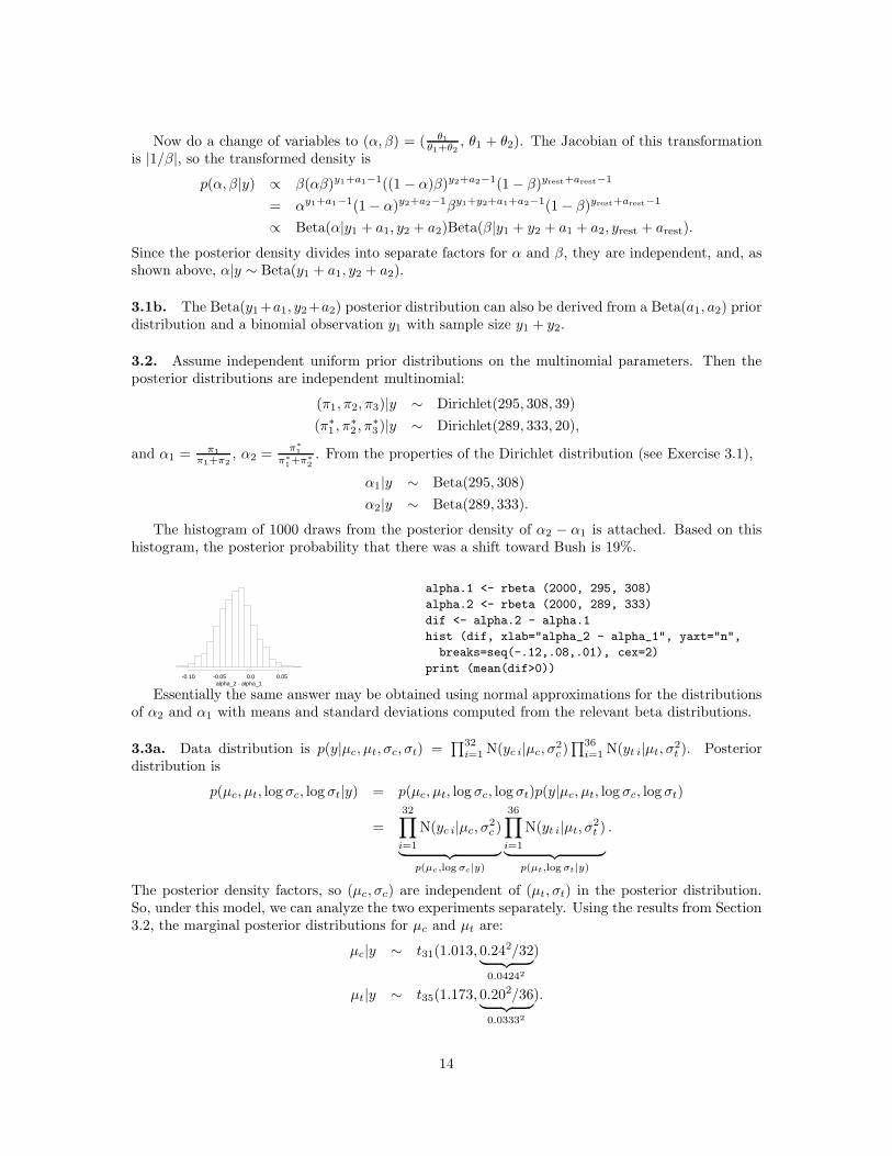
The histogram of 1000 draws from the posterior density of α2 − α1 is attached. Based on thishistogram, the posterior probability that there was a shift toward Bush is 19%.

-0.10 -0.05 0.0 0.05alpha_2 - alpha_1

alpha.1 <- rbeta (2000, 295, 308)

alpha.2 <- rbeta (2000, 289, 333)

dif <- alpha.2 - alpha.1

hist (dif, xlab="alpha_2 - alpha_1", yaxt="n",

breaks=seq(-.12,.08,.01), cex=2)

print (mean(dif>0))

Essentially the same answer may be obtained using normal approximations for the distributionsof α2 and α1 with means and standard deviations computed from the relevant beta distributions.

3.3a. Data distribution is p(y|µc, µt, σc, σt) =∏32

i=1 N(yc i|µc, σ2c )∏36

i=1 N(yt i|µt, σ2t ). Posterior

distribution is

p(µc, µt, log σc, log σt|y) = p(µc, µt, log σc, log σt)p(y|µc, µt, log σc, log σt)

=

32∏

i=1

N(yc i|µc, σ2c )

︸ ︷︷ ︸

p(µc,log σc|y)

36∏

i=1

N(yt i|µt, σ2t )

︸ ︷︷ ︸

p(µt,log σt|y)

.

The posterior density factors, so (µc, σc) are independent of (µt, σt) in the posterior distribution.So, under this model, we can analyze the two experiments separately. Using the results from Section3.2, the marginal posterior distributions for µc and µt are:

µc|y ∼ t31(1.013, 0.242/32

︸ ︷︷ ︸

0.04242

)

µt|y ∼ t35(1.173, 0.202/36

︸ ︷︷ ︸

0.03332

).

14

3.3b The histogram of 1000 draws from the posterior density of µt−µc is attached. Based on thishistogram, a 95% posterior interval for the average treatment effect is [0.05, 0.27].

-0.1 0.0 0.1 0.2 0.3 0.4mu_t - mu_c

mu.c <- 1.013 + (0.24/sqrt(32))*rt(1000,31)

mu.t <- 1.173 + (0.20/sqrt(36))*rt(1000,35)

dif <- mu.t - mu.c

hist (dif, xlab="mu_t - mu_c", yaxt="n",

breaks=seq(-.1,.4,.02), cex=2)

print (sort(dif)[c(25,976)])

3.5a. If the observations are treated as exact measurements then the theory of Section 3.2 applies.Then p(σ2|y) ∼ Inv-χ2(n− 1, s2) and p(µ|σ2, y) ∼ N(y, σ2/n) with n = 5, y = 10.4, s2 = 1.3.

3.5b. The posterior distribution assuming the non-informative prior distribution p(µ, σ2) ∝ 1/σ2

is

p(µ, σ2|y) ∝ 1

σ2

n∏

i=1

(

Φ

(yi + 0.5− µ

σ

)

− Φ

(yi − 0.5− µ

σ

))

,

where Φ is the standard normal cumulative distribution function.

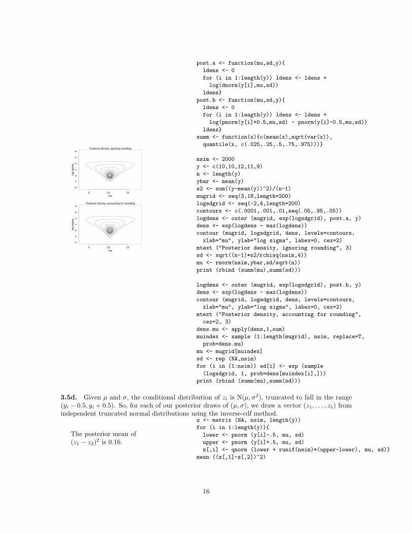
3.5c. We computed contour plots on a grid on the (µ, log σ) scale (levels are 0.0001, 0.001, 0.01,0.05–0.95). Draws from the posterior density in 3.5a can be obtained directly as described in Section3.2. Draws from the posterior density in 3.5b were obtained by sampling from the grid approximation(again using the (µ, log σ) scale).

mean sd 2.5% 25% 50% 75% 97.5%Ignoring roundingµ 10.4 0.74 8.9 10.1 10.4 10.8 11.8σ 1.4 0.74 0.68 0.98 1.2 1.6 3.3Accounting for roundingµ 10.5 0.69 9.2 10.1 10.4 10.8 11.8σ 1.4 0.73 0.61 0.90 1.2 1.6 3.3

The only notable difference is in the lower quantiles of σ.

15

mu

log

sigm

a

5 10 15

-2-1

01

23

4

Posterior density, ignoring rounding

mu

log

sigm

a

5 10 15

-2-1

01

23

4

Posterior density, accounting for rounding

post.a <- function(mu,sd,y){

ldens <- 0

for (i in 1:length(y)) ldens <- ldens +

log(dnorm(y[i],mu,sd))

ldens}

post.b <- function(mu,sd,y){

ldens <- 0

for (i in 1:length(y)) ldens <- ldens +

log(pnorm(y[i]+0.5,mu,sd) - pnorm(y[i]-0.5,mu,sd))

ldens}

summ <- function(x){c(mean(x),sqrt(var(x)),

quantile(x, c(.025,.25,.5,.75,.975)))}

nsim <- 2000

y <- c(10,10,12,11,9)

n <- length(y)

ybar <- mean(y)

s2 <- sum((y-mean(y))^2)/(n-1)

mugrid <- seq(3,18,length=200)

logsdgrid <- seq(-2,4,length=200)

contours <- c(.0001,.001,.01,seq(.05,.95,.05))

logdens <- outer (mugrid, exp(logsdgrid), post.a, y)

dens <- exp(logdens - max(logdens))

contour (mugrid, logsdgrid, dens, levels=contours,

xlab="mu", ylab="log sigma", labex=0, cex=2)

mtext ("Posterior density, ignoring rounding", 3)

sd <- sqrt((n-1)*s2/rchisq(nsim,4))

mu <- rnorm(nsim,ybar,sd/sqrt(n))

print (rbind (summ(mu),summ(sd)))

logdens <- outer (mugrid, exp(logsdgrid), post.b, y)

dens <- exp(logdens - max(logdens))

contour (mugrid, logsdgrid, dens, levels=contours,

xlab="mu", ylab="log sigma", labex=0, cex=2)

mtext ("Posterior density, accounting for rounding",

cex=2, 3)

dens.mu <- apply(dens,1,sum)

muindex <- sample (1:length(mugrid), nsim, replace=T,

prob=dens.mu)

mu <- mugrid[muindex]

sd <- rep (NA,nsim)

for (i in (1:nsim)) sd[i] <- exp (sample

(logsdgrid, 1, prob=dens[muindex[i],]))

print (rbind (summ(mu),summ(sd)))

3.5d. Given µ and σ, the conditional distribution of zi is N(µ, σ2), truncated to fall in the range

(yi − 0.5, yi + 0.5). So, for each of our posterior draws of (µ, σ), we draw a vector (z1, . . . , z5) fromindependent truncated normal distributions using the inverse-cdf method.

The posterior mean of(z1 − z2)

2 is 0.16.

z <- matrix (NA, nsim, length(y))

for (i in 1:length(y)){

lower <- pnorm (y[i]-.5, mu, sd)

upper <- pnorm (y[i]+.5, mu, sd)

z[,i] <- qnorm (lower + runif(nsim)*(upper-lower), mu, sd)}

mean ((z[,1]-z[,2])^2)

16

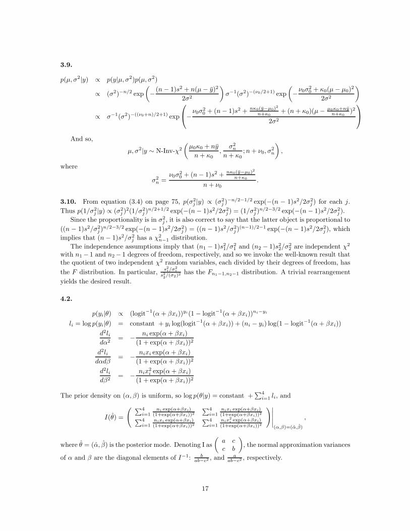
3.9.

p(µ, σ2|y) ∝ p(y|µ, σ2)p(µ, σ2)

∝ (σ2)−n/2 exp

(

− (n− 1)s2 + n(µ− y)2

2σ2

)

σ−1(σ2)−(ν0/2+1) exp

(

−ν0σ20 + κ0(µ− µ0)

2

2σ2

)

∝ σ−1(σ2)−((ν0+n)/2+1) exp

−ν0σ

20 + (n− 1)s2 + nκ0(y−µ0)

2

n+κ0

+ (n+ κ0)(µ− µ0κ0+nyn+κ0

)2

2σ2

And so,

µ, σ2|y ∼ N-Inv-χ2

(µ0κ0 + ny

n+ κ0,

σ2n

n+ κ0;n+ ν0, σ

2n

)

,

where

σ2n =

ν0σ20 + (n− 1)s2 + nκ0(y−µ0)

2

n+κ0

n+ ν0.

3.10. From equation (3.4) on page 75, p(σ2j |y) ∝ (σ2

j )−n/2−1/2 exp(−(n − 1)s2/2σ2

j ) for each j.

Thus p(1/σ2j |y) ∝ (σ2

j )2(1/σ2

j )n/2+1/2 exp(−(n− 1)s2/2σ2

j ) = (1/σ2j )

n/2−3/2 exp(−(n− 1)s2/2σ2j ).

Since the proportionality is in σ2j , it is also correct to say that the latter object is proportional to

((n − 1)s2/σ2j )

n/2−3/2 exp(−(n − 1)s2/2σ2j ) = ((n − 1)s2/σ2

j )(n−1)/2−1 exp(−(n − 1)s2/2σ2

j ), which

implies that (n− 1)s2/σ2j has a χ2

n−1 distribution.

The independence assumptions imply that (n1 − 1)s21/σ21 and (n2 − 1)s22/σ

22 are independent χ2

with n1 − 1 and n2− 1 degrees of freedom, respectively, and so we invoke the well-known result thatthe quotient of two independent χ2 random variables, each divided by their degrees of freedom, has

the F distribution. In particular,s21/σ2

1

s22/(σ2)2

has the Fn1−1,n2−1 distribution. A trivial rearrangement

yields the desired result.

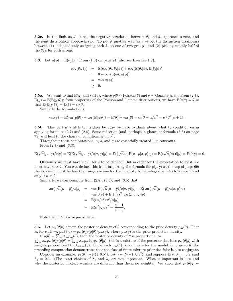
4.2.

p(yi|θ) ∝ (logit−1(α+ βxi))yi(1 − logit−1(α+ βxi))

ni−yi

li = log p(yi|θ) = constant + yi log(logit−1(α+ βxi)) + (ni − yi) log(1 − logit−1(α+ βxi))

d2lidα2

= − ni exp(α+ βxi)

(1 + exp(α+ βxi))2

d2lidαdβ

= − nixi exp(α+ βxi)

(1 + exp(α+ βxi))2

d2lidβ2

= − nix2i exp(α+ βxi)

(1 + exp(α+ βxi))2

The prior density on (α, β) is uniform, so log p(θ|y) = constant +∑4

i=1 li, and

I(θ) =

( ∑4i=1

ni exp(α+βxi)(1+exp(α+βxi))2

∑4i=1

nixi exp(α+βxi)(1+exp(α+βxi))2

∑4i=1

nixi exp(α+βxi)(1+exp(α+βxi))2

∑4i=1

nix2

i exp(α+βxi)(1+exp(α+βxi))2

)∣∣∣∣∣(α,β)=(α,β)

,

where θ = (α, β) is the posterior mode. Denoting I as

(a cc b

)

, the normal approximation variances

of α and β are the diagonal elements of I−1: bab−c2 , and

aab−c2 , respectively.

17

4.3. Let θ = LD50; we also introduce ν = β, in anticipation of a change of coordinates. Formula(4.1) on page 101 suggests that the (asymptotic) posterior median and mode should coincide, and the(asymptotic) posterior standard variance should be the inverse of observed information, evaluatedat the posterior mode.

With some effort (or using the “generalized linear model” function in a statistics package), itis possible to obtain decent numerical estimates for the posterior mode and standard deviationassociated with this data set; we will take these values as proxies for their asymptotic analogues.Here is one way to proceed:

Observe that p(θ|y) =∫p(θ, ν|y)dν =

∫p(α, β|y)|ν|dν, where α = −θν and β = ν in the last

integral, and |ν| is the Jacobian associated with the change in coordinates. (An expression forp(α, β|y) is given as (3.21) on page 90.

Fixing θ equal to a value around −0.12, which appears to be near the posterior mode (see Figure3.5 on page 93), we may compute

∫p(α, β|y)|ν|dν numerically (up to a proportionality constant that

does not depend on θ). The region of integration is infinite, but the integrand decays rapidly afterν passes 50, so that it suffices to estimate the integral assuming that ν runs from 0 to, say, 70.

This procedure can be repeated for several values of θ near −0.12. The values may be compareddirectly to find the posterior mode for θ. To three decimal places, we obtain −0.114.

One can fix a small value of h, such as h = 0.002, and estimate the d2/dθ2 log p(θ|y), evaluated at θequal to the posterior mode, by the expression [log p(−0.114+h|y)−2 logp(−0.114|y)+logp(−0.114−h|y)]/h2 (see (12.2) on page 314).

The negative of of the preceding quantity, taken to the −0.5 power, is our estimate for theposterior standard deviation. We get 0.096, which appears quite reasonable when compared toFigure 3.5, but which seems smaller than what we might guess from Figure 4.2(b). As remarkedon page 105, however, the actual posterior distribution of LD50 has less dispersion than what issuggested by Figure 4.2.

4.4. In the limit as n → ∞, the posterior variance approaches zero—that is, the posterior distri-bution becomes concentrated near a single point. Any one-to-one continuous transformation on thereal numbers is locally linear in the neighborhood of that point.

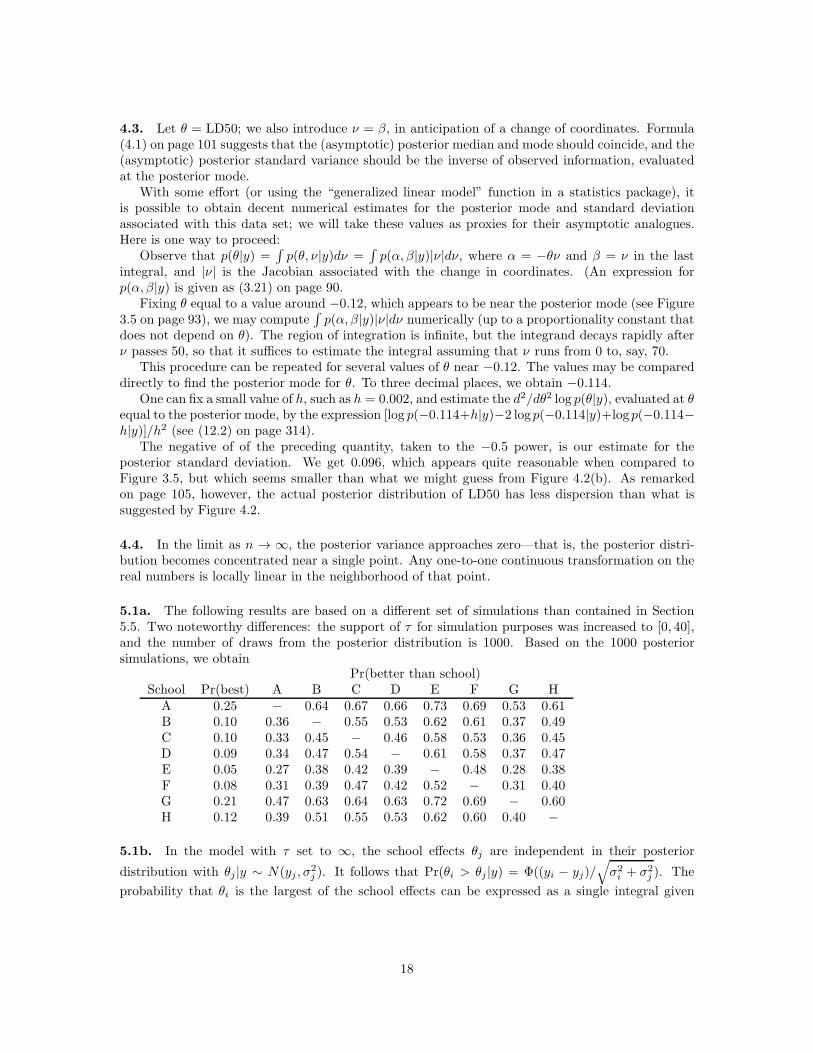
5.1a. The following results are based on a different set of simulations than contained in Section5.5. Two noteworthy differences: the support of τ for simulation purposes was increased to [0, 40],and the number of draws from the posterior distribution is 1000. Based on the 1000 posteriorsimulations, we obtain

Pr(better than school)School Pr(best) A B C D E F G H

A 0.25 − 0.64 0.67 0.66 0.73 0.69 0.53 0.61B 0.10 0.36 − 0.55 0.53 0.62 0.61 0.37 0.49C 0.10 0.33 0.45 − 0.46 0.58 0.53 0.36 0.45D 0.09 0.34 0.47 0.54 − 0.61 0.58 0.37 0.47E 0.05 0.27 0.38 0.42 0.39 − 0.48 0.28 0.38F 0.08 0.31 0.39 0.47 0.42 0.52 − 0.31 0.40G 0.21 0.47 0.63 0.64 0.63 0.72 0.69 − 0.60H 0.12 0.39 0.51 0.55 0.53 0.62 0.60 0.40 −

5.1b. In the model with τ set to ∞, the school effects θj are independent in their posterior

distribution with θj |y ∼ N(yj , σ2j ). It follows that Pr(θi > θj |y) = Φ((yi − yj)/

√

σ2i + σ2

j ). The

probability that θi is the largest of the school effects can be expressed as a single integral given

18

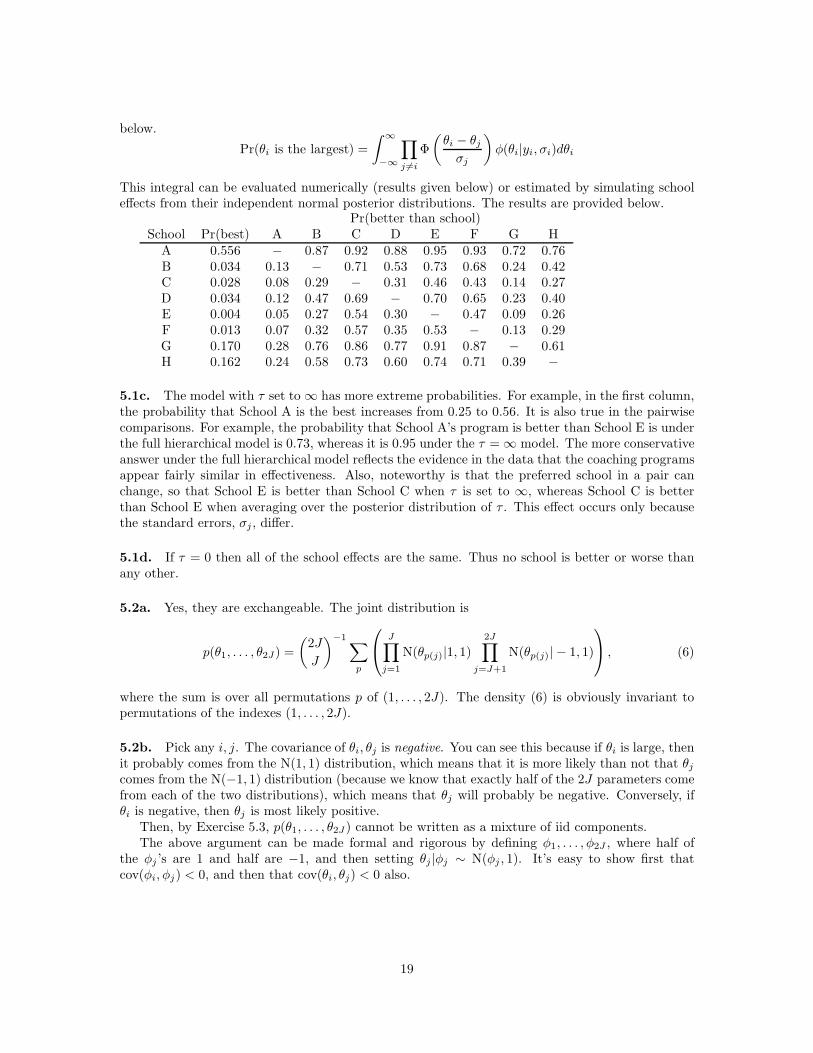
below.

Pr(θi is the largest) =

∫ ∞

−∞

∏

j 6=i

Φ

(θi − θjσj

)

φ(θi|yi, σi)dθi

This integral can be evaluated numerically (results given below) or estimated by simulating schooleffects from their independent normal posterior distributions. The results are provided below.

Pr(better than school)School Pr(best) A B C D E F G H

A 0.556 − 0.87 0.92 0.88 0.95 0.93 0.72 0.76B 0.034 0.13 − 0.71 0.53 0.73 0.68 0.24 0.42C 0.028 0.08 0.29 − 0.31 0.46 0.43 0.14 0.27D 0.034 0.12 0.47 0.69 − 0.70 0.65 0.23 0.40E 0.004 0.05 0.27 0.54 0.30 − 0.47 0.09 0.26F 0.013 0.07 0.32 0.57 0.35 0.53 − 0.13 0.29G 0.170 0.28 0.76 0.86 0.77 0.91 0.87 − 0.61H 0.162 0.24 0.58 0.73 0.60 0.74 0.71 0.39 −

5.1c. The model with τ set to ∞ has more extreme probabilities. For example, in the first column,the probability that School A is the best increases from 0.25 to 0.56. It is also true in the pairwisecomparisons. For example, the probability that School A’s program is better than School E is underthe full hierarchical model is 0.73, whereas it is 0.95 under the τ = ∞ model. The more conservativeanswer under the full hierarchical model reflects the evidence in the data that the coaching programsappear fairly similar in effectiveness. Also, noteworthy is that the preferred school in a pair canchange, so that School E is better than School C when τ is set to ∞, whereas School C is betterthan School E when averaging over the posterior distribution of τ . This effect occurs only becausethe standard errors, σj , differ.

5.1d. If τ = 0 then all of the school effects are the same. Thus no school is better or worse thanany other.

5.2a. Yes, they are exchangeable. The joint distribution is

p(θ1, . . . , θ2J) =

(2J

J

)−1∑

p

J∏

j=1

N(θp(j)|1, 1)2J∏

j=J+1

N(θp(j)| − 1, 1)

, (6)

where the sum is over all permutations p of (1, . . . , 2J). The density (6) is obviously invariant topermutations of the indexes (1, . . . , 2J).

5.2b. Pick any i, j. The covariance of θi, θj is negative. You can see this because if θi is large, thenit probably comes from the N(1, 1) distribution, which means that it is more likely than not that θjcomes from the N(−1, 1) distribution (because we know that exactly half of the 2J parameters comefrom each of the two distributions), which means that θj will probably be negative. Conversely, ifθi is negative, then θj is most likely positive.

Then, by Exercise 5.3, p(θ1, . . . , θ2J ) cannot be written as a mixture of iid components.The above argument can be made formal and rigorous by defining φ1, . . . , φ2J , where half of

the φj ’s are 1 and half are −1, and then setting θj |φj ∼ N(φj , 1). It’s easy to show first thatcov(φi, φj) < 0, and then that cov(θi, θj) < 0 also.

19

5.2c. In the limit as J → ∞, the negative correlation between θi and θj approaches zero, andthe joint distribution approaches iid. To put it another way, as J → ∞, the distinction disappearsbetween (1) independently assigning each θj to one of two groups, and (2) picking exactly half ofthe θj ’s for each group.

5.3. Let µ(φ) = E(θj |φ). From (1.8) on page 24 (also see Exercise 1.2),

cov(θi, θj) = E(cov(θi, θj |φ)) + cov(E(θi|φ),E(θj |φ))= 0 + cov(µ(φ), µ(φ))

= var(µ(φ))

≥ 0.

5.5a. We want to find E(y) and var(y), where y|θ ∼ Poisson(θ) and θ ∼ Gamma(α, β). From (2.7),E(y) = E(E(y|θ)); from properties of the Poisson and Gamma distributions, we have E(y|θ) = θ sothat E(E(y|θ)) = E(θ) = α/β.

Similarly, by formula (2.8),

var(y) = E(var(y|θ)) + var(E(y|θ)) = E(θ) + var(θ) = α/β + α/β2 = α/β2(β + 1).

5.5b. This part is a little bit trickier because we have to think about what to condition on inapplying formulas (2.7) and (2.8). Some reflection (and, perhaps, a glance at formula (3.3) on page75) will lead to the choice of conditioning on σ2.

Throughout these computations, n, s, and y are essentially treated like constants.From (2.7) and (3.3),

E(√n(µ−y)/s|y) = E(E(

√n(µ−y)/s|σ, y)|y) = E((

√n/s)E(µ−y|σ, y)|y) = E((

√n/s)·0|y) = E(0|y) = 0.

Obviously we must have n > 1 for s to be defined. But in order for the expectation to exist, wemust have n > 2. You can deduce this from inspecting the formula for p(µ|y) at the top of page 69:the exponent must be less than negative one for the quantity to be integrable, which is true if andonly if n > 2.

Similarly, we can compute from (2.8), (3.3), and (3.5) that

var(√n(µ− y)/s|y) = var(E(

√n(µ− y)/s|σ, y)|y) + E(var(

√n(µ− y)/s|σ, y)|y)

= var(0|y) + E((n/s2)var(µ|σ, y)|y)= E((n/s2)σ2/n|y)

= E(σ2|y)/s2 = n− 1

n− 3.

Note that n > 3 is required here.

5.6. Let pm(θ|y) denote the posterior density of θ corresponding to the prior density pm(θ). Thatis, for each m, pm(θ|y) = pm(θ)p(y|θ)/pm(y), where pm(y) is the prior predictive density.

If p(θ) =∑

m λmpm(θ), then the posterior density of θ is proportional to∑

m λmpm(θ)p(y|θ) =∑m λmpm(y)pm(θ|y): this is a mixture of the posterior densities pm(θ|y) withweights proportional to λmpm(y). Since each pm(θ) is conjugate for the model for y given θ, thepreceding computation demonstrates that the class of finite mixture prior densities is also conjugate.

Consider an example: p1(θ) ∼ N(1, 0.52), p2(θ) ∼ N(−1, 0.52), and suppose that λ1 = 0.9 amdλ2 = 0.1. (The exact choices of λ1 and λ2 are not important. What is important is how andwhy the posterior mixture weights are different than the prior weights.) We know that p1(θ|y) ∼

20

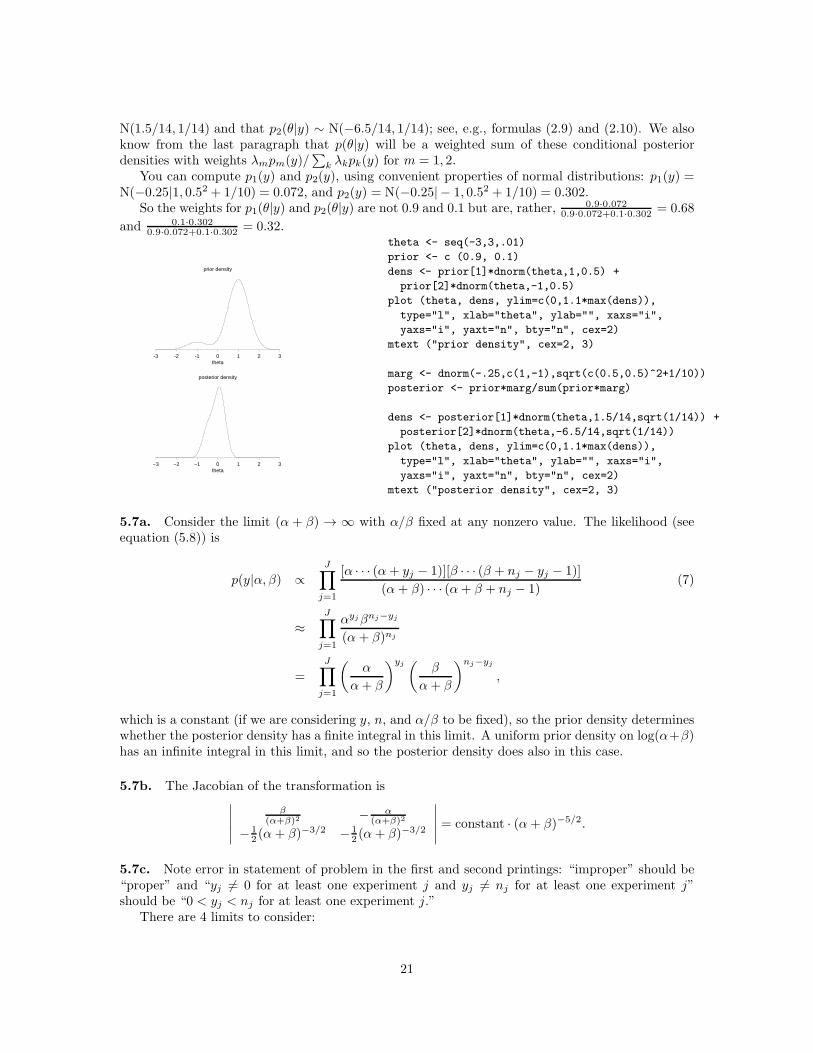
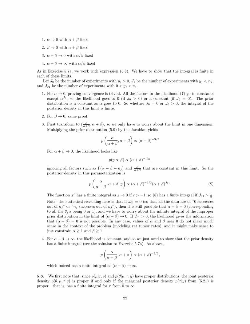
N(1.5/14, 1/14) and that p2(θ|y) ∼ N(−6.5/14, 1/14); see, e.g., formulas (2.9) and (2.10). We alsoknow from the last paragraph that p(θ|y) will be a weighted sum of these conditional posteriordensities with weights λmpm(y)/

∑

k λkpk(y) for m = 1, 2.You can compute p1(y) and p2(y), using convenient properties of normal distributions: p1(y) =

N(−0.25|1, 0.52 + 1/10) = 0.072, and p2(y) = N(−0.25| − 1, 0.52 + 1/10) = 0.302.So the weights for p1(θ|y) and p2(θ|y) are not 0.9 and 0.1 but are, rather, 0.9·0.072

0.9·0.072+0.1·0.302 = 0.68

and 0.1·0.3020.9·0.072+0.1·0.302 = 0.32.

theta-3 -2 -1 0 1 2 3

prior density

theta−3 −2 −1 0 1 2 3

posterior density

theta <- seq(-3,3,.01)

prior <- c (0.9, 0.1)

dens <- prior[1]*dnorm(theta,1,0.5) +

prior[2]*dnorm(theta,-1,0.5)

plot (theta, dens, ylim=c(0,1.1*max(dens)),

type="l", xlab="theta", ylab="", xaxs="i",

yaxs="i", yaxt="n", bty="n", cex=2)

mtext ("prior density", cex=2, 3)

marg <- dnorm(-.25,c(1,-1),sqrt(c(0.5,0.5)^2+1/10))

posterior <- prior*marg/sum(prior*marg)

dens <- posterior[1]*dnorm(theta,1.5/14,sqrt(1/14)) +

posterior[2]*dnorm(theta,-6.5/14,sqrt(1/14))

plot (theta, dens, ylim=c(0,1.1*max(dens)),

type="l", xlab="theta", ylab="", xaxs="i",

yaxs="i", yaxt="n", bty="n", cex=2)

mtext ("posterior density", cex=2, 3)

5.7a. Consider the limit (α + β) → ∞ with α/β fixed at any nonzero value. The likelihood (seeequation (5.8)) is

p(y|α, β) ∝J∏

j=1

[α · · · (α+ yj − 1)][β · · · (β + nj − yj − 1)]

(α+ β) · · · (α+ β + nj − 1)(7)

≈J∏

j=1

αyjβnj−yj

(α + β)nj

=J∏

j=1

(α

α+ β

)yj(

β

α+ β

)nj−yj

,

which is a constant (if we are considering y, n, and α/β to be fixed), so the prior density determineswhether the posterior density has a finite integral in this limit. A uniform prior density on log(α+β)has an infinite integral in this limit, and so the posterior density does also in this case.

5.7b. The Jacobian of the transformation is∣∣∣∣∣

β(α+β)2 − α

(α+β)2

− 12 (α + β)−3/2 − 1

2 (α+ β)−3/2

∣∣∣∣∣= constant · (α+ β)−5/2.

5.7c. Note error in statement of problem in the first and second printings: “improper” should be“proper” and “yj 6= 0 for at least one experiment j and yj 6= nj for at least one experiment j”should be “0 < yj < nj for at least one experiment j.”

There are 4 limits to consider:

21

1. α → 0 with α+ β fixed

2. β → 0 with α+ β fixed

3. α+ β → 0 with α/β fixed

4. α+ β → ∞ with α/β fixed

As in Exercise 5.7a, we work with expression (5.8). We have to show that the integral is finite ineach of these limits.

Let J0 be the number of experiments with yj > 0, J1 be the number of experiments with yj < nj ,and J01 be the number of experiments with 0 < yj < nj .

1. For α → 0, proving convergence is trivial. All the factors in the likelihood (7) go to constantsexcept αJ0 , so the likelihood goes to 0 (if J0 > 0) or a constant (if J0 = 0). The priordistribution is a constant as α goes to 0. So whether J0 = 0 or J0 > 0, the integral of theposterior density in this limit is finite.

2. For β → 0, same proof.

3. First transform to ( αα+β , α + β), so we only have to worry about the limit in one dimension.

Multiplying the prior distribution (5.9) by the Jacobian yields

p

(α

α+ β, α+ β

)

∝ (α+ β)−3/2

For α+ β → 0, the likelihood looks like

p(y|α, β) ∝ (α+ β)−J01 ,

ignoring all factors such as Γ(α + β + nj) and αα+β that are constant in this limit. So the

posterior density in this parameterization is

p

(α

α+ β, α+ β

∣∣∣∣y

)

∝ (α+ β)−3/2(α+ β)J01 . (8)

The function xc has a finite integral as x → 0 if c > −1, so (8) has a finite integral if J01 > 12 .

Note: the statistical reasoning here is that if J01 = 0 (so that all the data are of “0 successesout of nj” or “nj successes out of nj”), then it is still possible that α = β = 0 (correspondingto all the θj ’s being 0 or 1), and we have to worry about the infinite integral of the improperprior distribution in the limit of (α+ β) → 0. If J01 > 0, the likelihood gives the informationthat (α + β) = 0 is not possible. In any case, values of α and β near 0 do not make muchsense in the context of the problem (modeling rat tumor rates), and it might make sense tojust constrain α ≥ 1 and β ≥ 1.

4. For α+ β → ∞, the likelihood is constant, and so we just need to show that the prior densityhas a finite integral (see the solution to Exercise 5.7a). As above,

p

(α

α+ β, α+ β

)

∝ (α+ β)−3/2,

which indeed has a finite integral as (α+ β) → ∞.

5.8. We first note that, since p(µ|τ, y) and p(θ|µ, τ, y) have proper distributions, the joint posteriordensity p(θ, µ, τ |y) is proper if and only if the marginal posterior density p(τ |y) from (5.21) isproper—that is, has a finite integral for τ from 0 to ∞.

22

5.8a. Everything multiplying p(τ) in (5.21) approaches a nonzero constant limit as τ tends to zero;call that limit C(y). Thus the behavior of the posterior density near τ = 0 is determined by theprior density. The function p(τ) ∝ 1/τ is not integrable for any small interval including τ = 0, andso it leads to a nonintegrable posterior density. (We can make this more formal: for any δ > 0 wecan identify an interval including zero on which p(τ |y) ≥ p(τ)(C − δ).)

5.8b. The argument from 5.8a shows that if p(τ) ∝ 1 then the posterior density is integrable nearzero. We need to examine the behavior as τ → ∞ and find an upper bound that is integrable.The exponential term is clearly less than or equal to 1. We can rewrite the remaining terms as(∑J

j=1[∏

k 6=j(σ2k + τ2)])−1/2. For τ > 1 we make this quantity bigger by dropping all of the σ2 to

yield (Jτ2(J−1))−1/2. An upper bound on p(τ |y) for τ large is p(τ)J−1/2/τJ−1. When p(τ) ∝ 1,this upper bound is integrable if J > 2, and so p(τ |y) is integrable if J > 2.

5.8c. There are several reasonable options here. One approach is to abandon the hierarchical modeland just fit the two schools with independent noninformative prior distributions (as in Exercise 3.3but with the variances known).

Another approach would be to continue with the uniform prior distribution on τ and try toanalytically work through the difficulties with the resulting improper posterior distribution. In thiscase, the posterior distribution has all its mass near τ = ∞, meaning that no shrinkage will occurin the analysis (see (5.17) and (5.20)). This analysis is in fact identical to the first approach ofanalyzing the schools independently.

If the analysis based on noninformative prior distributions is not precise enough, it might beworthwhile assigning an informative prior distribution to τ (or perhaps to (µ, τ)) based on outsideknowledge such as analyses of earlier coaching experiments in other schools. However, one would haveto be careful here: with data on only two schools, inferences would be sensitive to prior assumptionsthat would be hard to check from the data at hand.

5.9a. p(θ, µ, τ |y) is proportional to p(θ, µ, τ)p(y|θ, µ, τ), where we may note that the latter densityis really just p(y|θ). Since p(θ, µ, τ) = p(θ|µ, τ)p(µ, τ),

p(θ, µ, τ |y) ∝ p(µ, τ)

J∏

j=1

[

θ−1j (1− θj)

−1τ−1 exp(−1

2(logit(θj)− µ)2/τ2)

] J∏

j=1

[θyj

j (1− θj)nj−yj

].

(The factor θ−1j (1 − θj)

−1 is d(logit(θj))/dθj ; we need this since we want to have p(θ|µ, τ) ratherthan p(logit(θ)|µ, τ).)

5.9b. Even though we can look at each of the J integrals individually—the integrand separatesinto independent factors—there is no obvious analytic technique which permits evaluation of theseintegrals. In particular, we cannot recognize a multiple of a familiar density function inside theintegrals. One might try to simplify matters with a substitution like uj = logit(θj) or vj = θj/(1−θj),but neither substitution turns out to be helpful.

5.9c. In order for expression (5.5) to be useful, we would have to know p(θ|µ, τ, y). Knowing it upto proportionality in θ is insufficient because our goal is to use this density to find another densitythat depends on µ and τ . In the rat tumor example (page 128, equation (5.7)), the conjugacy ofthe beta distribution allowed us to write down the relevant “constant” of proportionality, which ofcourse appears in equation (5.8).

23

5.10 Following the hint we apply (2.7) and (2.8).

E(θj |τ, y) = E[E(θj |µ, τ, y) | τ, y] = E

1σ2

j

yj +1τ2µ

1σ2

j

+ 1τ2

∣∣∣∣∣τ, y

=

1σ2

j

yj +1τ2 µ

1σ2

j

+ 1τ2

var(θj |τ, y) = E[var(θj |µ, τ, y) | τ, y] + var[E(θj |µ, τ, y) | τ, y] =1

1σ2

j

+ 1τ2

+

1τ2

1σ2

j

+ 1τ2

2

Vµ,

where expressions for µ = E(µ|τ, y) and Vµ = var(µ|τ, y) are given in (5.20) of Section 5.4.

6.1a. Under the model that assumes identical effects in all eight schools (τ = 0), the posteriordistribution for the common θ is N(7.9, 4.22); see page 139–140. To simulate the posterior predictivedistribution of yrep we first simulate θ ∼ N(7.9, 4.22) and then simulate yrepj ∼ N(θ, σ2

j ) for j =1, . . . , 8. The observed order statistics would be compared to the distribution of the order statisticsobtained from the posterior predictive simulations. The expected order statistics provided in theproblem (from a N(8, 132) reference distribution) are approximately the mean order statistics wewould find in the replications. (The mean in the replications would differ because the school standarderrors vary and because the value 13 does not incorporate the variability in the common θ.)

Just by comparing the observed order statistics to the means provided, it is clear that theidentical-schools model does fit this aspect of the data. Based on 1000 draws from the posteriorpredictive distribution we find that observed order statistics correspond to upper-tail probabilitiesranging from 0.20 to 0.62, which further supports the conclusion.

6.1b. It is easy to imagine that we might be interested in choosing some schools for further studyor research on coaching programs. Under the identical-effects model, all schools would be equallygood for such follow-up studies. However, most observers would wish to continue experimenting inSchool A rather than School C.

6.1c. The decision to reject the identical-effects model was based on the notion that the posteriordistribution it implies (all θj ’s the same) does not make substantive sense.

6.5.

1. A “hypothesis of no difference” probably refers to a hypothesis that θ = 0 or θ1 = θ2 in somemodel. In this case, we would just summarize our uncertainty about the parameters using theposterior distribution, rather than “testing” the hypothesis θ = 0 or θ1 = θ2 (see, for example,Exercises 3.2–3.4). The issue is not whether θ is exactly zero, but rather what we know aboutθ.

2. One can also think of a model itself as a hypothesis, in which case the model checks describedin this chapter are hypothesis tests. In this case, the issue is not whether a model is exactlytrue, but rather what are the areas where the model (a) does not fit the data, and (b) issensitive to questionable assumptions. The outcome of model checking is not “rejection” or“acceptance,” but rather an exploration of the weak points of the model. With more data, wewill be able to find more weak points. It is up to the modeler to decide whether an area inwhich the model does not fit the data is important or not (see page 366 for an example).

24

6.6a. Under the new protocol,

p(y, n|θ) =n∏

i=1

θyi(1 − θ)1−yi1∑n−1

i=1(1−yi)=12

1∑n

i=1(1−yi)=13

For the given data, this is just θ7(1 − θ)13, which is the likelihood for these data under the “stopafter 20 trials” rule. So if the prior distribution for θ is unchanged, then the posterior distributionis unchanged.

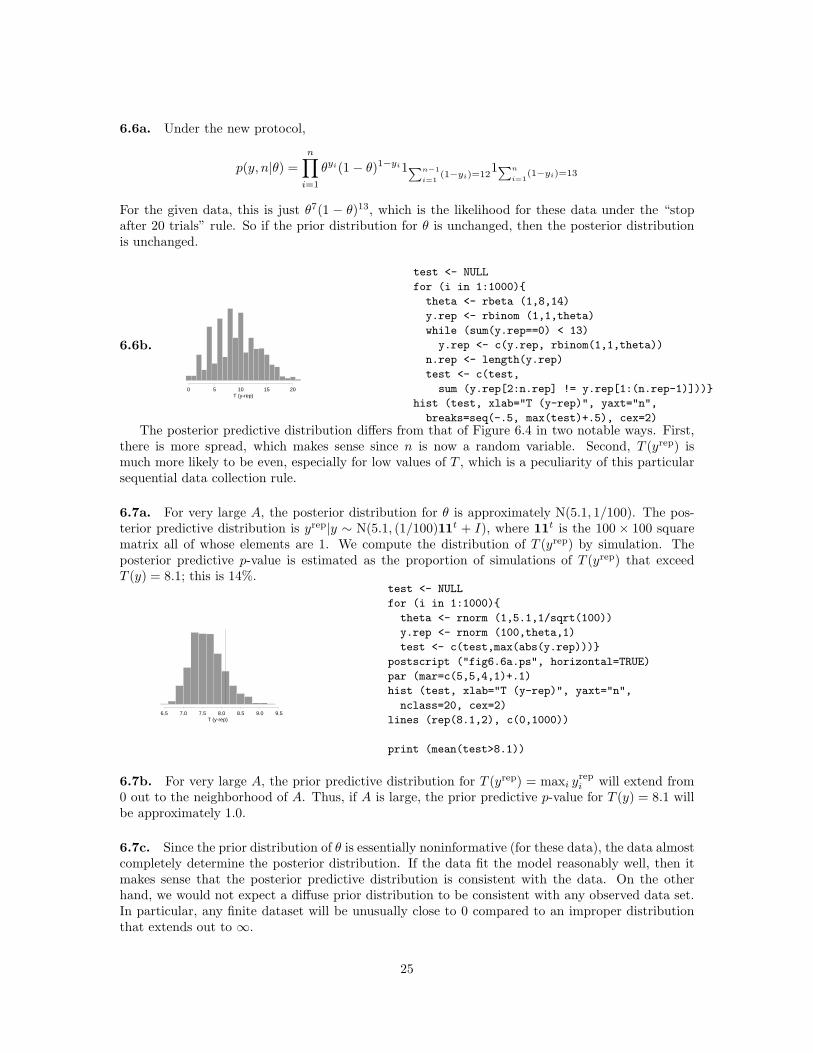
6.6b.

0 5 10 15 20T (y-rep)

test <- NULL

for (i in 1:1000){

theta <- rbeta (1,8,14)

y.rep <- rbinom (1,1,theta)

while (sum(y.rep==0) < 13)

y.rep <- c(y.rep, rbinom(1,1,theta))

n.rep <- length(y.rep)

test <- c(test,

sum (y.rep[2:n.rep] != y.rep[1:(n.rep-1)]))}

hist (test, xlab="T (y-rep)", yaxt="n",

breaks=seq(-.5, max(test)+.5), cex=2)The posterior predictive distribution differs from that of Figure 6.4 in two notable ways. First,

there is more spread, which makes sense since n is now a random variable. Second, T (yrep) ismuch more likely to be even, especially for low values of T , which is a peculiarity of this particularsequential data collection rule.

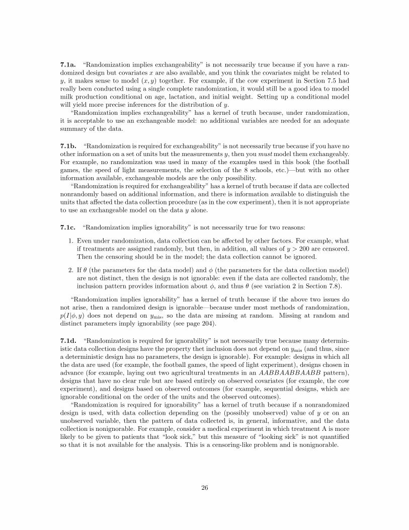
6.7a. For very large A, the posterior distribution for θ is approximately N(5.1, 1/100). The pos-terior predictive distribution is yrep|y ∼ N(5.1, (1/100)11t + I), where 11t is the 100 × 100 squarematrix all of whose elements are 1. We compute the distribution of T (yrep) by simulation. Theposterior predictive p-value is estimated as the proportion of simulations of T (yrep) that exceedT (y) = 8.1; this is 14%.

6.5 7.0 7.5 8.0 8.5 9.0 9.5T (y-rep)

test <- NULL

for (i in 1:1000){

theta <- rnorm (1,5.1,1/sqrt(100))

y.rep <- rnorm (100,theta,1)

test <- c(test,max(abs(y.rep)))}

postscript ("fig6.6a.ps", horizontal=TRUE)

par (mar=c(5,5,4,1)+.1)

hist (test, xlab="T (y-rep)", yaxt="n",

nclass=20, cex=2)

lines (rep(8.1,2), c(0,1000))

print (mean(test>8.1))

6.7b. For very large A, the prior predictive distribution for T (yrep) = maxi yrepi will extend from

0 out to the neighborhood of A. Thus, if A is large, the prior predictive p-value for T (y) = 8.1 willbe approximately 1.0.

6.7c. Since the prior distribution of θ is essentially noninformative (for these data), the data almostcompletely determine the posterior distribution. If the data fit the model reasonably well, then itmakes sense that the posterior predictive distribution is consistent with the data. On the otherhand, we would not expect a diffuse prior distribution to be consistent with any observed data set.In particular, any finite dataset will be unusually close to 0 compared to an improper distributionthat extends out to ∞.

25

7.1a. “Randomization implies exchangeability” is not necessarily true because if you have a ran-domized design but covariates x are also available, and you think the covariates might be related toy, it makes sense to model (x, y) together. For example, if the cow experiment in Section 7.5 hadreally been conducted using a single complete randomization, it would still be a good idea to modelmilk production conditional on age, lactation, and initial weight. Setting up a conditional modelwill yield more precise inferences for the distribution of y.

“Randomization implies exchangeability” has a kernel of truth because, under randomization,it is acceptable to use an exchangeable model: no additional variables are needed for an adequatesummary of the data.

7.1b. “Randomization is required for exchangeability” is not necessarily true because if you have noother information on a set of units but the measurements y, then youmustmodel them exchangeably.For example, no randomization was used in many of the examples used in this book (the footballgames, the speed of light measurements, the selection of the 8 schools, etc.)—but with no otherinformation available, exchangeable models are the only possibility.

“Randomization is required for exchangeability” has a kernel of truth because if data are collectednonrandomly based on additional information, and there is information available to distinguish theunits that affected the data collection procedure (as in the cow experiment), then it is not appropriateto use an exchangeable model on the data y alone.

7.1c. “Randomization implies ignorability” is not necessarily true for two reasons:

1. Even under randomization, data collection can be affected by other factors. For example, whatif treatments are assigned randomly, but then, in addition, all values of y > 200 are censored.Then the censoring should be in the model; the data collection cannot be ignored.

2. If θ (the parameters for the data model) and φ (the parameters for the data collection model)are not distinct, then the design is not ignorable: even if the data are collected randomly, theinclusion pattern provides information about φ, and thus θ (see variation 2 in Section 7.8).

“Randomization implies ignorability” has a kernel of truth because if the above two issues donot arise, then a randomized design is ignorable—because under most methods of randomization,p(I|φ, y) does not depend on ymis, so the data are missing at random. Missing at random anddistinct parameters imply ignorability (see page 204).

7.1d. “Randomization is required for ignorability” is not necessarily true because many determin-istic data collection designs have the property thet inclusion does not depend on ymis (and thus, sincea deterministic design has no parameters, the design is ignorable). For example: designs in which allthe data are used (for example, the football games, the speed of light experiment), designs chosen inadvance (for example, laying out two agricultural treatments in an AABBAABBAABB pattern),designs that have no clear rule but are based entirely on observed covariates (for example, the cowexperiment), and designs based on observed outcomes (for example, sequential designs, which areignorable conditional on the order of the units and the observed outcomes).

“Randomization is required for ignorability” has a kernel of truth because if a nonrandomizeddesign is used, with data collection depending on the (possibly unobserved) value of y or on anunobserved variable, then the pattern of data collected is, in general, informative, and the datacollection is nonignorable. For example, consider a medical experiment in which treatment A is morelikely to be given to patients that “look sick,” but this measure of “looking sick” is not quantifiedso that it is not available for the analysis. This is a censoring-like problem and is nonignorable.

26

7.1e. “Ignorability implies exchangeability” is not necessarily true for the same reason as theanswer to Exercise 7.1a. Even if you are allowed to use an exchangeable model on y, you might stilldo better by modeling (x, y), even if x is not used in the data collection.

“Ignorability implies exchangeability” has a kernel of truth because, if the data collection isignorable given yobs, so that it does not depend on other variables x, then it is not necessary toinclude x in the analysis: one can apply an exchangeable model to y.

7.1f. “Ignorability is required for exchangeability” is not necessarily true: consider censored datacollection (for example, variation 3 in Section 7.8). The design is nonignorable, and the inclusionpattern must be included in the model, but the model is still exchangeable in the yobs i’s.

“Ignorability is required for exchangeability” has a kernel of truth because if the data collectionis nonignorable given yobs, and additional information x is available that is informative with respectto the data collection, then x should be included in the model because p(θ|x, yobs, I) 6= p(θ|yobs).This is an exchangeable model on (x, y), not y.

7.2. Many possibilities: for example, in the analysis of the rat tumor experiments in Chapter 5, weare assuming that the sample sizes, nj , provide no information about the parameters θj—this is likethe assumption of distinct parameters required for ignorability. But one could imagine situations inwhich this is not true—for example, if more data are collected in labs where higher tumor rates areexpected. This would be relevant for the parameter of interest, y71, because n71 has the relativelylow value of 14. One way the analysis could reflect this possibility is to model θj conditional on nj .To do this would be awkward using the beta distribution on the θj ’s; it might be easier to set up alogistic regression model—basically, a hierarchical version of the model in Section 3.7. This wouldtake a bit of computational and modeling effort—before doing so, it would make sense to plot theestimated θj ’s vs. the nj ’s to see if there seems to be any relation between the variables.

7.7a. We can write the posterior distribution of µ, σ as,

σ2|yobs ∼ Inv-χ2(n− 1, s2)

µ|σ2, yobs ∼ N(yobs, σ2/n),

where yobs and s2 are the sample mean and variance of the n data points yobsi .The predictive distribution of the mean of the missing data is,

ymis|µ, σ2, yobs ∼ N(µ, σ2/(N − n)).

Averaging over µ yields,

ymis|σ2, yobs ∼ N(yobs, (1/n+ 1/(N − n))σ2).

Since σ2 has an inverse-χ2 posterior distribution, averaging over it yields a t distribution (as on p.76):

ymis|yobs ∼ tn−1(yobs, (1/n+ 1/(N − n))s2).

The complete-data mean is y = n/Nyobs + (N − n)/Nymis, which is a linear transformation ofymis (trating n, N , and yobs as constants, since they are all observed) and so it has a t posteriordistribution also:

y|yobs ∼ tn−1(yobs, s2(1/n+ 1/(N − n))(N − n)2/N2)

= tn−1(yobs, s2(N − n)/(nN))

= tn−1(yobs, s2(1/n− 1/N)).

27

7.7b. The t distribution with given location and scale parameters tends to the correspondingnormal distribution as the degrees of freedom go to infinity:

Since (1 + z/w)w → exp(z) as w → ∞, the expression (1/σ)(1 + (1/ν)((θ − µ)/σ)2)−(ν+1)/2

approaches (1/σ) exp(− 12 ((θ − µ)/σ)2) as ν → ∞.

7.15a. The assignment for the current unit depends on previous treatment assignments. Thus, thetime sequence of the assignments must be recorded. This can be expressed as a covariate as ti foreach observation i, where ti = 1, 2, . . .. A time covariate giving the actual times (not just the timeorder) of the observations would be acceptable also (that is, the design would be ignorable giventhis covariate) and, in practice, might make it easier to model the outcomes, given t.

7.15b. If the outcome is y = (y1, . . . , yn), we would model it as (y|x, θ), along with a prior distribu-tion, p(θ|x), where θ describes all the parameters in the model and x are the covariates, which mustinclude the treatment assignment and the time variable (and can also include any other covariatesof interest, such as sex, age, medical history, etc.).

7.15c. Under this design, inferences are sensitive to dependence of y on t (conditional on θ andthe other variables in x). If such dependence is large, it needs to be modeled, or the inferenceswill not be appropriate. Under this design, t plays a role similar to a blocking variable or thepre-treatment covariates in the milk production example in Section 7.5. For example, suppose thatE(y|x, θ) has a linear trend in t but that this dependence is not modeled (that is, suppose that amodel is fit ignoring t). Then posterior means of treatment effects will tend to be reasonable, butposterior standard deviations will be too large, because this design yields treatment assignmentsthat, compared to complete randomization, tend to be more balanced for t.

7.15d. Under the proposed design and alternative (ii), you must include the times t as one of thecovariates in your model; under alternative (i), it is not necessary to include t. This is an advantageof alternative (i), since it reduces the data collection requirements. On the other hand, it couldbe considered an advantage of the proposed design and alternative (ii), since it forces you to usethis information, which may very well lead to more relevant inferences (if, for example, treatmentefficacy increases with t).

Suppose that, under all three designs, you will model the data using the same set of covariatesx (that include treatment assignment and t). Of the three designs, alternative (ii) is most balancedfor t, alternative (i) is least balanced (on average), and the proposed design falls in between. So,assuming smooth changes in the dependence of y on t (conditional on x and θ), we would expectdata collected under alternative (ii) to yield the most precise inferences and under alternative (i)the least precise. If for some reason there was an alternating trend (for example, if the patients areassigned to two doctors, and the doctors tend to alternate), then alternative (ii) could become theleast precise.

Another potential difficulty in alternative (ii) is posterior predictive model checking (or, in clas-sical terms, hypothesis testing). Since this alternative has only two possible treatment vectors, it isbasically impossible to check the fit of the model under replications of the treatment under the samepatients. (It would be, however, possible to test the fit of the model as it would apply to additionalpatients.)

8.1. We assume for simplicity that the posterior distribution is continuous and that needed mo-ments exist. The proofs can be easily adapted to discontinuous distributions.

28

8.1a. The calculus below shows that L(a|y) has zero derivative at a = E(θ|y). Also the secondderivative is positive so this is a minimizing value.

d

daE(L(a|y)) = d

da

∫

(θ − a)2p(θ|y)dθ = −2

∫

(θ − a)p(θ|y)dθ = −2(E(θ|y)− a) = 0 if a = E(θ|y).

8.1b. We can apply the argument from 4.5c with ko = k1 = 1.

8.1c. The calculus below shows that L(a|y) has zero derivative at any a for which∫ a

−∞p(θ|y)dθ =

k0/(k0 + k1). Once again the positive second derivative indicates that it is a minimizing value.

d

daE(L(a|y)) =

d

da

(∫ a

−∞

k1(a− θ)p(θ|y)dθ +∫ ∞

a

k0(θ − a)p(θ|y)dθ)

= k1

∫ a

−∞

p(θ|y)dθ − k0

∫ ∞

a

p(θ|y)dθ

= (k1 + k0)

∫ a

−∞

p(θ|y)dθ − k0.

8.2. Denote the posterior mean by m(y) = E(θ|y) and consider m(y) as an estimator of θ.Unbiasedness implies that E(m(y)|θ) = θ. In this case, the marginal expectation of θm(y) isE(θm(y)) = E[E(θm(y)|θ)] = E[θ2]. But we can also write E(θm(y)) = E[E(θm(y)|y)] = E[m(y)2].It follows that E[(m(y) − θ)2] = 0. This can only hold in degenerate problems for which m(y) = θwith probability 1.

8.4. Our goal is to show that, for sufficiently large sigma, the “Bayes estimate” (the posterior meanof θ based on the prior density p(θ) = 1 in [0, 1]) has lower mean squared error than the maximumlikelihood estimate, for any value of θ ∈ [0, 1].

The maximum likelihood estimate, restricted to the interval [0, 1], takes value 0 with probabilityΦ(−c/σ) and takes value 1 with probability 1−Φ((1−c)/σ); these are just the probabilities (given σand θ) that y is less than 0 or greater than 1, respectively. For very large σ, these probabilities bothapproach Φ(0) = 1/2. Thus, for very large σ, the mean squared error of the maximum likelihoodestimate is approximately 1/2[(1 − θ)2 + θ2] = 1/2 − θ + θ2. (We use the notation Φ for the unitnormal cumulative distribution function.)

On the other hand, p(θ|y) is proportional to the density function N(θ|y, σ2) for θ ∈ [0, 1]. The

posterior mean of θ, E(θ|y), is∫ 1

0θN(θ|y, σ2)dθ/

∫ 1

0p(θ|y, σ)dθ. For very large σ, N(θ|y, σ2) is

approximately constant over small ranges of θ (e.g., over [0, 1]). So the Bayes estimate is close to∫ 1

0 θdθ = 1/2. (This works because, since the true value of θ is assumed to lie in [0, 1], the observedy will almost certainly lie within a few standard deviations of 1/2.) Hence, for large σ, the meansquared error of the posterior mean is about (θ − 1/2)2 = 1/4− θ + θ2.

The difference in (asymptotic, as σ → ∞) mean squared errors is independent of the true value ofθ. Also, for large σ the maximum likelihood estimate generally chooses 0 or 1, each with probabilityalmost 1/2, whereas the Bayes estimate chooses 1/2 with probability almost 1.

8.6. This is a tricky problem.For this to work out, given the form of θ, the prior distribution should be a mixture of a spike

at θ = 0 and a flat prior distribution for θ 6= 0. It’s easy to get confused with degenerate andnoninformative prior distributions, so let’s write it as

p(θ) = λN(θ|0, τ21 ) + (1− λ)N(θ|0, τ22 ),

29

work through the algebra, and then take the limit τ1 → 0 (so that θ = 0 is a possibility) and τ2 → ∞(so that θ = y is a possibility).

We’ll have to figure out the appropriate limit for λ by examining the posterior distribution:

p(θ|y) ∝ p(θ)N(y|θ, σ2/n)

∝ λN(θ|0, τ21 )N(y|θ, σ2/n) + (1 − λ)N(θ|0, τ22 )N(y|θ, σ2/n)

∝ λN(y|0, τ21 + σ2/n)N

(

θ

∣∣∣∣∣

nσ2 y

2

1τ2

1

+ nσ2

,1

1τ2

1

+ nσ2

)

+

(1− λ)N(y|0, τ22 + σ2/n)N

(

θ

∣∣∣∣∣

nσ2 y

2

1τ2

2

+ nσ2

,1

1τ2

2

+ nσ2

)

This is a mixture of two normal densities. In the limit τ1 → 0 and τ2 → ∞, this is

p(θ|y) = λN(y|0, σ2/n)N(θ|0, τ21 ) + (1− λ)N(y|0, τ22 )N(θ|y, σ2/n).

The estimate θ cannot be the posterior mean (that would not make sense, since, as defined, θis a discontinuous function of y). Since the two normal densities have much different variances, itwould also not make sense to use a posterior mode estimate. A more reasonable estimate (if a pointestimate must be used) is the mode of the hump of the posterior distribution that has greater mass.That is,

Set θ = 0 if: λN(y|0, σ2/n) > (1− λ)N(y|0, τ22 )

λ1

√

2π/nσexp

(

−1

2

n

σ2y2)

> (1− λ)1√2πτ2

, (9)

and set θ = y otherwise.For condition (9) to be equivalent to “if y < 1.96σ/

√n,” as specified, we must have

0.146λ1

√

2π/nσ= (1− λ)

1√2πτ2

λ

1− λ=

σ

0.146√nτ2

.

Since we are considering the limit τ2 → ∞, this means that λ → 0. That would be acceptable (akind of improper prior distribution), but the more serious problem here is that the limiting value forλτ2 depends on n, and thus the prior distribution for θ depends on n. A prior distribution cannotdepend on the data, so there is no prior distribution for which the given estimate θ is a reasonableposterior summary.

8.8. There are many possible answers here; for example:

(a) With a weak prior distribution, why bother with Bayesian inference? Because it is a directway to get inferences for quantities of interest. For instance, in the examples of Sections 3.5and 3.7, the Bayesian inference is straightforward. Why not use Bayesian inference in theseexamples? Is there a method that gives better results?

(b) With a strong prior distribution, why collect new data? This question misses the point, becauseany strong prior distribution must come from lots of previous data (as in the example of thesex ratio of births in Chapter 2) or a theoretical model, or some combination of the two. Ifenough previous data have been collected to form a precise inference, then new data may be

30

collected in order to see whether the model generalizes to other situations. For example, inthe placenta previa example of Section 2.5, we cannot really use the data from all previousbirths in Germany to construct an extremely strong prior distribution—we have to be open tothe possibility that the new data will have a different rate of female births.

(c) With something in between, does Bayesianism “duck the issue”? The “issue” here is: whatshould the relative weights be for the prior and data? Bayesian inference sets these weightsfor different cases based on the availability of data, as is explained for the cancer rate examplein Section 2.8.

The issue is further clarified in Chapter 5. In each of the three examples in Chapter 5, thereare multiple experiments, each run under slightly different conditions and with a relativelysmall sample size. Using an informative—but not extremely strong—prior distribution allowsus to get better inferences for the result of each individual experiment. The Bayesian methoddoes not “duck the issue” because the relative weights given to the prior distribution and thedata are determined by the data themselves.

11.1a. Suppose that θ is drawn from the density proportional to g(θ), and U is a random Uniform(0, 1)draw. Then we can express the cumulative distribution function of draws accepted by rejection sam-pling as

Pr(θ ≤ θ∗|θ is accepted) =Pr(θ ≤ θ∗ and U ≤ p(θ|y)

Mg(θ) )

Pr(U ≤ p(θ|y)Mg(θ) )

=

∫ θ∗

−∞

∫ p(θ|y)/(Mg(θ))

0 g(θ)dudθ∫∞

−∞

∫ p(θ|y)/(Mg(θ))

0g(θ)dudθ

=1M

∫ θ∗

−∞ p(θ|y)dθ1M

,

which is the cumulative density function for p(θ|y).A similar argument works in higher dimensions.

11.1b. The above proof requires that (i) g(θ) > 0 wherever p(θ) > 0 (otherwise the final integralwill not cover the support of p) and that (ii) p(θ)/Mg(θ) ≤ 1 always (otherwise the integral over uwill have the range of [0, 1] rather than [0, p/Mg], and the transition to the last line of the equationwill not be valid). If p/g is unbounded, than one or both of (i) and (ii) will be violated.

11.2. As described at the top of p. 291: consider any two points θa and θb, at iteration t labeledso that p(θb|y)Jt(θa|θb) ≥ p(θa|y)Jt(θb|θa). To show that the posterior distribution is a stationarydistribution, suppose that θt−1 is a draw from the posterior distribution. Then the unconditionalprobability density of a transition from θa to θb is

p(θt−1=θa, θt=θb) = p(θa|y)Jt(θb|θa),

where the acceptance probability is 1 because of our labeling of a and b so that the ratio of importanceratios is at least 1. The unconditional probability density of a transition from θb to θa is

p(θt=θa, θt−1=θb) = p(θb|y)Jt(θa|θb)

(p(θa|y)/Jt(θa|θb)p(θb|y)/Jt(θb|θa)

)

,

which is the same as the unconditional probability in the other direction. Since their joint distribu-tion is symmetric, θt and θt−1 have the same marginal distributions, and so p(θ|y) is a stationarydistribution of the Markov chain.

31

As with the Metropolis algorithm, the stationary distribution is unique if the Markov chain isirreducible, aperiodic, and not transient.

12.6. We find the conditional posterior distribution of γ = log σ by transforming the inverse-χ2.

p(γ|θ, µ, τ, y) ∝ 2e2γ(e−2γ)n/2+1e−nσ2/2e2γ .

Maximizing the log of this density (which is equivalent to maximizing the density) yields γ = log σ.The argument for log τ is similar.

12.7. The joint posterior density is given by the formula on page 300. If θj = µ for all j, then theexpression simplifies to

p(θ, µ, log σ, log τ |y) ∝ τ(√2πτ)−J

J∏

j=1

nj∏

i=1

N(yij |θj , σ2)

= (2π)−J/2τ−(J−1)J∏

j=1

nj∏

i=1

N(yij |θj , σ2).

This is just τ−(J−1) multiplied by a function of the other parameters and the data. In this case,J = 4, so as τ → 0 with θj = µ for all j, the joint posterior density is proportional to τ−3, whichapproaches infinity.

14.1a. We fit a linear regression with a uniform prior density on (β, log σ). We include coefficientsfor the basement indicator and for three county indicators, and no constant term. (If data on morecounties were available, or if we were interested in forecasting for additional counties, then we wouldfit a hierarchical regression at the county level, as discussed in Chapter 15.)

Posterior quantilesQuantity of interest 25% 50% 75%

geometric mean for Blue Earth (no basement), exp(β2) 4.1 5.0 6.5geometric mean for Blue Earth County (basement), exp(β1 + β2) 6.1 7.1 8.2geometric mean for Clay County (no basement), exp(β3) 3.8 4.7 5.8geometric mean for Clay County (basement), exp(β1 + β3) 5.6 6.5 7.6geometric mean for Goodhue County (no basement), exp(β4) 3.9 4.9 6.2geometric mean for Goodhue County (basement), exp(β1 + β4) 5.8 6.8 7.9factor for basement vs. no basement, exp(β1) 1.1 1.4 1.7geometric sd of predictions, exp(σ) 2.1 2.2 2.4

All estimates in the table come from the S code below: applying the normal regression model tothe logarithms of the data, drawing 1000 simulations of (β, σ), and then computing quantiles of thequantities of interest.

Nontechnical summary: The first six lines of the above table gives stimates and uncertaintiesfor the average county radon level (separating into houses without and with basements). Theserange from about 4 to 8 pCi/L. Within a county, the houses with basements have, on average, radonlevels between 10% and 70% higher than houses without basements. One can expect the radonmeasurement in any given house to vary by about a factor of 2.2 from the mean of houses of thesame “basement status” in the same county.

make.indicators <- function (x){

ux <- unique(x)

32

mat1 <- matrix (x, nrow=length(x), ncol=length(ux))

mat2 <- matrix (ux, nrow=length(x), ncol=length(ux), byrow=T)

(mat1==mat2)*1}

y.1 <- c (5.0, 13.0, 7.2, 6.8, 12.8, 5.8, 9.5, 6.0, 3.8, 14.3, 1.8, 6.9, 4.7, 9.5)

y.2 <- c (0.9, 12.9, 2.6, 3.5, 26.6, 1.5, 13.0, 8.8, 19.5, 2.5, 9.0, 13.1, 3.6, 6.9)

y.3 <- c (14.3, 6.9, 7.6, 9.8, 2.6, 43.5, 4.9, 3.5, 4.8, 5.6, 3.5, 3.9, 6.7)

basement.1 <- c(1,1,1,1,1,0,1,1,1,0,1,1,1,1)

basement.2 <- c(0,1,1,0,1,1,1,1,1,0,1,1,1,0)

basement.3 <- c(1,0,1,0,1,1,1,1,1,1,1,1,1)

counties <- rep(1:3,c(length(y.1),length(y.2),length(y.3)))

y <- c(y.1,y.2,y.3)

x <- cbind (c(basement.1,basement.2,basement.3), make.indicators(counties))

ls.out <- lsfit (x, log(y), intercept=F)

lsd <- ls.diag (ls.out)

nsim <- 10000

n <- nrow(x)

k <- ncol(x)

sigma <- rep (NA, nsim)

beta <- array (NA, c(nsim, k))

for (i in 1:nsim){

sigma[i] <- lsd$std.dev*sqrt((n-k)/rchisq(1,n-k))

beta[i,] <- ls.out$coef + (sigma[i]/lsd$std.dev)*lsd$std.err*t(chol(lsd$corr))%*%rnorm(k)}

output <- exp (cbind (beta[,2], beta[,1]+beta[,2], beta[,3],

beta[,1] + beta[,3], beta[,4], beta[,1] + beta[,4], beta[,1], sigma))

for (i in 1:ncol(output)) print (round(quantile(output[,i],c(.25,.5,.75)),1))

14.1b. Let y be the radon measurement in the new house, b be the variable that equals 1 if thehouse has a basement, and c be the county where the house is located. We are given c. Then wecan draw from the posterior predictive distribution of y in four steps:

1. Draw (β, σ2) from the posterior distribution as in Exercise 8.1a.

2. Draw b from the posterior distribution p(b|c).

3. Draw log y from the conditional posterior distribution p(log y|b, c) from the regression modelin Exercise 8.1a (N(β3, σ

2) if b = 0 or N(β1 + β3, σ2) if b = 1).

4. Compute y = exp(log y).

To perform step 2 above, we need a model for b|c. Let θc be the proportion of houses in BlueEarth County that have basements. For simplicity, we shall assume a binomial model (equivalent toassuming simple random sampling of houses within each county, and a large population of housesrelative to the sample size), so that bi|ci ∼ Bernoulli, (θc), for each house i in this county. We also,for simplicity, assume a uniform prior distribution on θc. The posterior distribution for θc is thenBeta(3, 13). So we draw b by first drawing θc ∼ Beta(3, 13), then drawing b ∼ Bernoulli(θc).

0 10 20 30 40radon measurement (new house)

theta <- rbeta (nsim, 3, 13)

b <- rbinom (nsim, 1, theta)

logy.rep <- rnorm (nsim, beta[,3] + b*beta[,1], sigma)

y.rep <- exp(logy.rep)

print (round(quantile(y.rep,c(.025,.25,.5,.75,.975)),1))

hist (y.rep[y.rep<40], yaxt="n", breaks=0:40,

xlab="radon measurement (new house)", cex=2)

The 2.5%, 25%, 50%, 75%, and 97.5% posterior quantiles for y are 0.8, 2.8, 5.1, 9.0, and 33.3. Tomake the histogram readable, we omit the approximately 2% of simulated values that are greaterthan 40.

33

14.3. Assuming p(β|σ) = p(β) to be uniform, we have p(β|σ, y) proportional to p(y|β, σ), that is,to exp(− 1

2 (y −Xβ)t(y −Xβ)/σ2). This posterior density is an exponential of a quadratic form inβ and hence is normal.

To show: the mean is β = (XtX)−1Xty and the variance is (XtX)−1σ2.It suffices to demonstrate that the following two quantities are equal (up to additive terms not

depending on β, which correspond to multiplicative constants in the posterior density function):

(y −Xβ)t(y −Xβ) and (β − β)tXtX(β − β).Expanding the quadratics, (y − Xβ)t(y − Xβ) = −βtXty − ytXβ + βtXtXβ + constant, and

(β − β)tXtX(β − β) = βtXtXβ − ytX(XtX)−1(XtX)β − βt(XtX)(XtX)−1Xty + constant =βtXtXβ − ytXβ − βtXty + constant, which establishes (14.4) and (14.5).

14.4. p(σ2|y) = p(β, σ2|y)/p(β|σ2, y). Assuming a prior density p(β, σ2) = p(β)p(σ2) = σ−2 and

fixing β at the value β on the right side of this equation, we get something proportional to

σ−(n+2) exp(− 12 (y −Xβ)t(y −Xβ)/σ2)

(det((XtX)−1σ2))−1/2 exp(0). (10)

Note that det((XtX)−1σ2) = σ2kdet((XtX)−1), since XtX has dimension k, and this expression

is σ2k times a constant. Thus (10) is proportional in σ to σ−(n−k+2) exp(− 12σ

−2(y − Xβ)t(y −Xβ)/σ2).

Comparing this result to the scaled inverse-χ2 density in Appendix A reveals that our posteriordensity is, in fact, inverse-χ2(n− k, s2).

14.7. First write the joint distribution of everything, p(β, log σ, y, y) = N(y|β, σ2I)N(y|β, σ2I).Now consider y and σ to be constants (that is, condition on them). The joint density is then aquadratic function in (β, y). So (β, y) jointly have a normal distribution, which means that themarginal distribution of y is also normal (see Appendix A).

17.1a. Conditional on the parameters µ1, τ1, λ1, µ2, τ2, λ2 (which are assumed known for this prob-lem), the posterior distribution is

p(θ|y) ∝8∏

j=1

2∑

m=1

λmN(θj |µm, τ2m)N(yj |θj , σ2j ).

We use the fact that

N(θ|µ, τ2)N(y|θ, σ2) = N(y|µ, σ2 + τ2)N

(

θ

∣∣∣∣

1τ2µ+ 1

σ2 y1τ2 + 1

σ2

,1

1τ2 + 1

σ2

)

.

(This is based on the identity p(θ)p(y|θ) = p(y, θ) = p(y)p(θ|y) for the normal model.) We can thenwrite the posterior distribution for the mixture model as

p(θ|y) ∝8∏

j=1

2∑

m=1

λ∗mjN

θj

∣∣∣∣∣∣

1τ2mµm + 1

σ2

j

yj

1τ2m

+ 1σ2

j

,1

1τ2m

+ 1σ2

j

,

where

λ∗mj =

λmN(yj |µm, σ2j + τ2m)

λ1N(yj |µ1, σ2j + τ21 ) + λ2N(yj |µ2, σ2

j + τ22 )for m = 1, 2.

For the given parameter values and the data in Table 5.2, the posterior distributions are independentand are as follows:

34

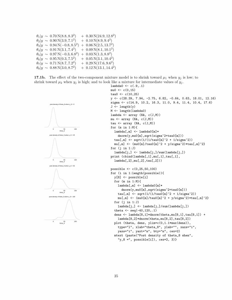
θ1|y ∼ 0.70N(8.8, 8.32) + 0.30N(24.9, 12.82)θ2|y ∼ 0.90N(3.9, 7.12) + 0.10N(8.9, 9.42)θ3|y ∼ 0.94N(−0.8, 8.52) + 0.06N(2.5, 13.72)θ4|y ∼ 0.91N(3.1, 7.42) + 0.09N(8.1, 10.12)θ5|y ∼ 0.97N(−0.3, 6.82) + 0.03N(1.3, 8.82)θ6|y ∼ 0.95N(0.3, 7.52) + 0.05N(3.1, 10.42)θ7|y ∼ 0.71N(8.7, 7.22) + 0.29N(17.6, 9.62)θ8|y ∼ 0.88N(3.0, 8.72) + 0.12N(13.1, 14.42)

17.1b. The effect of the two-component mixture model is to shrink toward µ1 when yj is low; toshrink toward µ2 when yj is high; and to look like a mixture for intermediate values of yj .

theta_80 50 100

post density of theta_8 when y_8 = 0

theta_80 50 100

post density of theta_8 when y_8 = 25

theta_80 50 100

post density of theta_8 when y_8 = 50

theta_80 50 100

post density of theta_8 when y_8 = 100

lambda0 <- c(.9,.1)

mu0 <- c(0,15)

tau0 <- c(10,25)

y <- c(28.39, 7.94, -2.75, 6.82, -0.64, 0.63, 18.01, 12.16)

sigma <- c(14.9, 10.2, 16.3, 11.0, 9.4, 11.4, 10.4, 17.6)

J <- length(y)

M <- length(lambda0)

lambda <- array (NA, c(J,M))

mu <- array (NA, c(J,M))

tau <- array (NA, c(J,M))

for (m in 1:M){

lambda[,m] <- lambda0[m]*

dnorm(y,mu0[m],sqrt(sigma^2+tau0[m]))

tau[,m] <- sqrt(1/(1/tau0[m]^2 + 1/sigma^2))

mu[,m] <- (mu0[m]/tau0[m]^2 + y/sigma^2)*tau[,m]^2}

for (j in 1:J)

lambda[j,] <- lambda[j,]/sum(lambda[j,])

print (cbind(lambda[,1],mu[,1],tau[,1],

lambda[,2],mu[,2],tau[,2]))

possible <- c(0,25,50,100)

for (i in 1:length(possible)){

y[8] <- possible[i]

for (m in 1:M){

lambda[,m] <- lambda0[m]*

dnorm(y,mu0[m],sqrt(sigma^2+tau0[m]))

tau[,m] <- sqrt(1/(1/tau0[m]^2 + 1/sigma^2))

mu[,m] <- (mu0[m]/tau0[m]^2 + y/sigma^2)*tau[,m]^2}

for (j in 1:J)

lambda[j,] <- lambda[j,]/sum(lambda[j,])

theta <- seq(-40,120,.1)

dens <- lambda[8,1]*dnorm(theta,mu[8,1],tau[8,1]) +

lambda[8,2]*dnorm(theta,mu[8,2],tau[8,2])

plot (theta, dens, ylim=c(0,1.1*max(dens)),

type="l", xlab="theta_8", ylab="", xaxs="i",

yaxs="i", yaxt="n", bty="n", cex=2)

mtext (paste("Post density of theta_8 when",

"y_8 =", possible[i]), cex=2, 3)}

35