SICE Journal of Control, Measurement, and System Integration, Vol. 10, No. 3, pp. 141–148, May 2017

Special Issue on SICE Annual Conference 2016

Some Improvements in Elastoplastic Friction Compensator1

Masayoshi IWATANI ∗ and Ryo KIKUUWE ∗

Abstract : For robotic joints with compliant transmissions, Mahvash and Okamura have proposed a friction compensatorbased on an elastoplastic friction model. One drawback of the compensator is that the compensator continues producingnon-zero output force in the static friction state, which results in the degraded backdrivability of joints. In order to remedythis problem, this paper proposes an elastoplastic friction compensator with improved static friction behavior, which isrealized by an additional term that makes the output force exponentially decay in the static friction state. This paper alsoproposes an additional algorithm that adjust the decay rate of the output force in real time. The proposed methods areexperimentally tested with a linear actuator with a timing belt and a six-axis industrial manipulator.

Key Words : friction compensation, static friction, dither.

1. Introduction

In robotic systems, joint friction is one of major factors thatdegrade the backdrivability of the joint and the accuracy of con-trol. One straightforward idea to handle this problem is frictioncompensation, i.e., generating actuator force canceling the fric-tion force. To find an appropriate compensator, however, is nota trivial problem. One major factor of the difficulty is that thefriction force is generally formulated as a discontinuous func-tion of the sliding velocity. Inappropriate treatment of the dis-continuities leads to high frequency oscillation in the actuatorforce in the neighborhood of the zero velocity.

One of the simplest friction models is Hayward and Arm-strong’s [2] friction model. Their friction model can be seenas an elastoplastic friction model, which is composed of a se-rial connection of an elastic component and a Coulomb-frictioncomponent. Some other friction models can be seen as ex-tensions of Hayward and Armstrong’s model. For example,Dupont et al.’s model [3] is an elastoplastic friction model witha sophisticated presliding behavior. Kikuuwe et al. [4] haveproposed a viscoelasto-plastic model, which includes non-zeroviscosity in the presliding region. Xiong et al.’s model [5] isa multi-state friction model, which is composed of multipleviscoelasto-plastic elements connected in parallel.

The originally intended application of Hayward and Arm-strong’s elastoplastic friction model [2] is haptic rendering, inwhich artificial friction forces are generated by the actuators.Mahvash and Okamura [6], however, employed their model forthe purpose of friction compensation, in which the real fric-tion forces are canceled by the actuator forces. They appliedtheir technique for a tendon-driven mechanism, in which thecompliance of the tendon corresponds to the compliance of theelastoplastic friction model. A similar idea has also been em-ployed by the authors [7], in which a multi-state viscoelasto-

∗ Department of Mechanical Engineering, Kyushu University,744 Motooka, Nishi-ku, Fukuoka, 819-0395, JapanE-mail: iwatani@ctrl.mech.kyushu-u.ac.jp, kikuuwe@mech.kyushu-u.ac.jp(Received October 25, 2016)(Revised December 17, 2016)

1 This paper extends the authors’ previous conference paper [1].

plastic friction model was used for friction compensation of aharmonic drive transmission. Tjahjowidodo et al. [8] also de-veloped a friction compensator for a harmonic drive based on amulti-state friction model [9].

In this paper, we focus on a flaw of the elastoplastic fric-tion compensators, which has not been pointed out in previousstudies. The flaw is that, in the static friction state, the com-pensator continues generating non-zero actuator force causedby the imaginary elastic displacement in the compensator. Thisunnecessary output force hampers the sensitivity of the jointagainst the external force. Motivated by this observation, thispaper proposes an improved elastoplastic friction compensator,which includes an additional term that makes the output forceexponentially decay in the static friction state. We also com-bine this new method with a sinusoidal dither-like actuation inthe static friction state to further enhance the sensitivity of thesystem against external forces. Moreover, we propose an addi-tional algorithm for the compensator, with which the decay rateof the output force is adjusted in real time to realize a betterbehavior of the system both kinetic and static friction states.

The content of the paper has been partially presented in ourprior conference publication [1]. Newly added contribution ofthe present paper is the new additional algorithm that adjuststhe decay rate and new experimental results obtained with anindustrial manipulator with harmonic-drive transmissions.

The rest of this paper is organized as follows. Section 2shows our experimental setups. Section 3 overviews Mahvashand Okamura’s elastoplastic friction compensator. Section 4presents a new elastoplastic friction compensator, which alle-viates the flaw of Mahvash and Okamura’s method. Section 5shows experimental results of the proposed compensator. Sec-tion 6 presents the additional algorithm for the online adjust-ment of the decay rate, and also shows some experimental re-sults. Section 7 provides some concluding remarks.

2. Experimental Setups

2.1 Overview

Experiments in this paper employ two experimental devices,which are shown in Fig. 1. Setup A, shown in Fig. 1 (a), consistsof an AC servomotor, in which an optical encoder is embedded,

JCMSI 0003/17/1003–0141 c© 2016 SICE

SICE JCMSI, Vol. 10, No. 3, May 2017142

Fig. 1 Experimental setups.

Fig. 2 Schematic illustration of the setups.

and a ball screw connected through a timing belt and pulleysto the servomotor. In this device, the end-effector and the ac-tuator are connected through a compliant transmission, i.e., thetiming belt. Setup B, shown in Fig. 1 (b), is a six-axis indus-trial manipulator MOTOMAN-HP3J, Yaskawa Electric Corpo-ration. Each joint of the setup has an AC servomotor, an opticalencoder and a harmonic drive transmission, which has compli-ance.

In each of the setups, the friction mostly exists on the end-effector’s side, not on the actuator and the optical encoder’sside. This feature raises a difficulty in the friction compensationbecause the end-effector’s velocity cannot be measured directlywith the optical encoder.

The mechanism structures of the setups can be schematicallyillustrated as in Fig. 2. Here, p and qc represent the position ofthe actuator and the end-effector, respectively, Kc is the elastic-ity of the compliant transmission, f f is the friction force on theside of the end-effector, f is the force of the actuator, and fe isexternal forces acting on the end-effector. This arrangement ofthe friction and the compliance is the same as that of Mahvashand Okamura [6], where a tendon-driven joint is modeled in thesame way as Fig. 2.

As for Setup A, the linear actuator, the rated power of the

Fig. 3 Presliding properties of the setups.

Fig. 4 Identification result of rate-dependent friction.

actuator is 200 W, the lead of the ball screw is 0.02 m, andthe resolution of the encoder is 4000 counts per rotation. Asfor Setup B, the industrial manipulator, we used only the threejoints from the base. In these three joints (Joints 0, 1 and 2),all the actuators’ rated power is 80 W, and all the encoders’ res-olution is 65, 536 counts per rotation, and the reduction ratiosof the transmissions are 100, 224 and 120, respectively. Dur-ing the experiments, a force sensor NITTA IFS-50M31A25-I25was attached to the end-effector of each setup to measure theexternal forces.

2.2 Presliding Behaviors

Preliminary experiments were performed to clarify the pre-sliding behaviors of our setups. In these experiments, ramp-type force input was applied to the joints by the actuators. Fig-ure 3 shows the result. Figure 3 (a) shows that the measureddisplacement of Setup A is zero as long as the actuator forceis smaller than 6 N. On the other hand, in Fig. 3 (b), Joint 0 ofMOTOMAN-HP3J exhibits significant presliding displacementunder small actuator torque.

SICE JCMSI, Vol. 10, No. 3, May 2017 143

The difference of the presliding behaviors between the twosetups can be attributed to the differences in the stiffness of thetransmission and the resolution of the encoders. In the case ofSetup A, due to the high stiffness of the timing belt, the elon-gation of the belt was smaller than displacement for one countof the encoder step. On the other hand in the case of Setup B,the resolution of the encoder is high enough to observe smalldisplacement under small torque.

2.3 Identification of Rate-Dependent Friction

In order to investigate the relation between the velocity andthe friction force in our setups, we used our previously pro-posed procedure [10], which is for the identification of rate-dependent friction law. The procedure was slightly modifiedto deal with different magnitudes of friction in different direc-tions. Figure 4 shows the obtained data and curves from theprocedure. Here we describes the curves in the following form:

f ∈ gsgn(−Fn, v, Fp) + Φ(v) (1)

where Fp and Fn are positive constants, Φ(·) is a continuousfunction that satisfies Φ(0) = 0, and gsgn is the generalizedsignum function defined as follows:

gsgn(A, x, B)Δ=

⎧⎪⎪⎪⎪⎨⎪⎪⎪⎪⎩B if x > 0

[A, B] if x = 0A if x < 0.

(2)

The function Φ(·) and the constants Fp and Fn are obtainedby the linear interpolation and extrapolation of the sampledvelocity-friction force pairs. Figure 4 (a) shows that, in SetupA, the magnitudes of friction are different in different direc-tions, i.e., Fp � Fn, and the curve of the rate-dependent frictionis almost straight. Figure 4 (b) shows that, in Setup B, the mag-nitude of friction is almost symmetric with respect to velocityv = 0. We use the identified Fp, Fn and Φ(·) in the proposedcompensator.

3. Previous Elastoplastic Friction Compensator

3.1 Friction Model on Which Previous Compensator IsBased

Hayward and Armstrong’s elastoplastic friction model [2] isa serial connection of an elastic element and a Coulomb frictionelement. Their model is originally presented in the discrete-time domain. In their model, the algorithm to obtain the frictionforce fk from the input position pk, where k is the discrete-timeindex, can be written as follows:

qk := pk − FK

sat(K

F(pk − qk−1)

)(3a)

fk := K(pk − qk) (3b)

where sat(·) is a unit saturation function defined as follows:

sat(x)Δ=

{x/|x| if |x| > 1x if |x| ≤ 1.

(4)

Here, F represents the magnitude of the Coulomb friction force,K represents the spring coefficient of the elastic element, andqk is a state variable representing the position of the Coulombfriction element.

Kikuuwe et al.’s [4] friction model is also presented in thediscrete-time domain and can be seen as a generalization of the

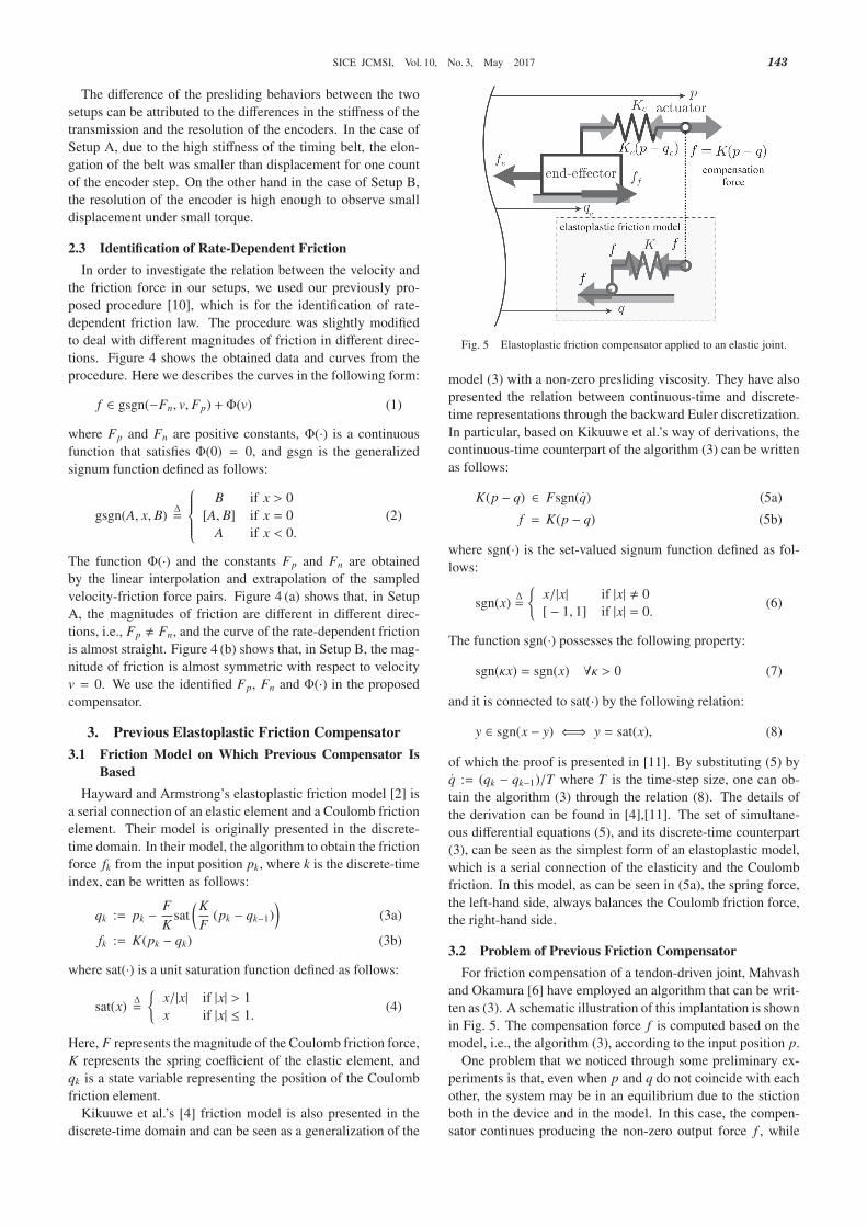
Fig. 5 Elastoplastic friction compensator applied to an elastic joint.

model (3) with a non-zero presliding viscosity. They have alsopresented the relation between continuous-time and discrete-time representations through the backward Euler discretization.In particular, based on Kikuuwe et al.’s way of derivations, thecontinuous-time counterpart of the algorithm (3) can be writtenas follows:

K(p − q) ∈ Fsgn(q) (5a)

f = K(p − q) (5b)

where sgn(·) is the set-valued signum function defined as fol-lows:

sgn(x)Δ=

{x/|x| if |x| � 0[ − 1, 1] if |x| = 0.

(6)

The function sgn(·) possesses the following property:

sgn(κx) = sgn(x) ∀κ > 0 (7)

and it is connected to sat(·) by the following relation:

y ∈ sgn(x − y) ⇐⇒ y = sat(x), (8)

of which the proof is presented in [11]. By substituting (5) byq := (qk − qk−1)/T where T is the time-step size, one can ob-tain the algorithm (3) through the relation (8). The details ofthe derivation can be found in [4],[11]. The set of simultane-ous differential equations (5), and its discrete-time counterpart(3), can be seen as the simplest form of an elastoplastic model,which is a serial connection of the elasticity and the Coulombfriction. In this model, as can be seen in (5a), the spring force,the left-hand side, always balances the Coulomb friction force,the right-hand side.

3.2 Problem of Previous Friction Compensator

For friction compensation of a tendon-driven joint, Mahvashand Okamura [6] have employed an algorithm that can be writ-ten as (3). A schematic illustration of this implantation is shownin Fig. 5. The compensation force f is computed based on themodel, i.e., the algorithm (3), according to the input position p.

One problem that we noticed through some preliminary ex-periments is that, even when p and q do not coincide with eachother, the system may be in an equilibrium due to the stictionboth in the device and in the model. In this case, the compen-sator continues producing the non-zero output force f , while

SICE JCMSI, Vol. 10, No. 3, May 2017144

the end-effector stays in the static friction state. This situa-tion is not preferable because, to break away this static frictionstate, an external force fe larger than the static friction levelmay be required. That is, in the static friction state, the outputof the compensator degrades the device’s sensitivity to externalforces.

4. Proposed Friction Compensator4.1 Main Contribution: Exponentially Decaying Output

Force

Here we present a new friction compensator that avoids theproblem explained in Section 3.2. The source of the problemis the dislocated equilibrium between p and q, which results inthe continuing non-zero output force f in the static friction. Inorder to prevent this, we propose a modified version of (5) asfollows:

K(p − q) ∈ Fsgn (q + α(q − p)) (9a)

f = K(p − q) (9b)

where α is a positive constant.In the compensator (9), the additional term +α(q− p) has the

effect of preventing the equilibrium at q − p � 0. Equation (9a)can be equivalently rewritten as follows:

((K(p − q) = F) ∧ (q + α(q − p) > 0))

∨ ((|K(p − q)| < F) ∧ (q + α(q − p) = 0))

∨ ((K(p − q) = −F) ∧ (q + α(q − p) < 0)) , (10)

which can be further rewritten as follows:

((q > αF/K) ∧ (K(p − q) = F))

∨ ((q = −α(q − p)) ∧ (|K(p − q)| < F))

∨ ((q < −αF/K) ∧ (K(p − q) = −F)) . (11)

This implies that, when K(p − q) = f ∈ (−F, F), i.e., when thecompensator is in the static friction state, q exponentially con-verges to p and the parameter α determines the rate of conver-gence. Meanwhile, when K(p − q) = f is either +F or −F,i.e., when the compensator is in the kinetic friction state, thevelocity q is larger than αF/K. That is, the parameter α deter-mines the threshold value αF/K above which the compensatorproduces a constant force. The former effect indeed preventsthe dislocated equilibrium at p � q although the latter effect isnot what we exactly intended.

Here we derive the algorithm of the compensator based onthe simultaneous differential equations (9). The backward Eulerdiscretization of (9a) can be written as follows:

K(pk − qk) ∈ Fsgn(qk − qk−1

T+ α (qk − pk)

), (12)

which is equivalent to

KF

(pk − qk) ∈ sgn

(K (pk − qk−1)F (1 + Tα)

− KF

(pk − qk)

). (13)

By the application of the relation (8), one can see that (13) isequivalent to the following:

KF

(pk − qk) = sat

(K (pk − qk−1)F (1 + Tα)

), (14)

which is equivalent to

qk = pk − FK

sat

(K (pk − qk−1)F (1 + Tα)

). (15)

Consequently, the discrete-time algorithm of the proposed fric-tion compensator is written as follows:

qk := pk − FK

sat

(K(pk − qk−1)F(1 + Tα)

)(16a)

fk := K(pk − qk). (16b)

The compensator (16) is built on the assumption that the de-vice friction is the pure Coulomb friction, i.e., f = Fsgn(v).If the friction force is rate-dependent as in (1) and Fig. 4, thecontinuous-time representation of the compensator (9) shouldbe slightly generalized as follows:

K(p − q) ∈ gsgn(−Fn, q + α(q − p), Fp

)(17a)

f = K(p − q) + Φ(q). (17b)

A straightforward derivation shows that, through the backwardEuler discretization, a discrete-time algorithm correspondent to(17) can be obtained as follows:

qk := pk − 1K

gsat

(−Fn,

K(pk − qk−1)1 + Tα

, Fp

)(18a)

f := K(pk − qk) + Φ(qk − qk−1

T

). (18b)

Here, gsat is a generalized saturation function defined as fol-lows:

gsat(A, x, B)Δ=

⎧⎪⎪⎪⎪⎨⎪⎪⎪⎪⎩B if x > Bx if x ∈ [A, B]A if x < A,

(19)

and the following properties of gsgn and gsat are used in thederivation:

gsgn(A, κx, B) = gsgn(A, x, B) ∀κ > 0 (20)

y ∈ gsgn(A, x − y, B) ⇐⇒ y = gsat(A, x, B). (21)

The functions gsgn and gsat have been introduced in [11] wherea proof for the relation (21) is also included.

The performance of the algorithm (18) cannot be very sensi-tive to the choice of the time-step size T because both functionsgsat and Φ are continuous and thus the algorithm does not in-volve any discontinuities. The parameter α should be chosenaccording to the required convergence rate of the compensationforce. Note that α is not a model parameter of the controlledobject, but a design parameter that should be chosen accordingto the purposes of applications.

4.2 Algorithm

The output force f of the algorithm (16), or its generalizedversion (18), exponentially decays to zero during the static fric-tion state. Therefore, it does not facilitate the breaking awayfrom the static friction state according to external forces belowthe maximum static friction level. Thus, we combine the al-gorithm (18) with a dither-like actuation that is activated onlyin the static friction state. The purpose here is to improve thesystem’s sensitivity to external forces by maintaining the sys-tem on the verge of the static friction state. We choose a simplesinusoidal signal for the dither actuation, and its amplitude ischosen so that it causes oscillation of a few encoder counts.

SICE JCMSI, Vol. 10, No. 3, May 2017 145

The frequency of the signal is chosen so that it is higher thanthe supposed frequency component of the external force. In ourcase, because we are considering the application in which therobot is manually moved by human hand, it is set higher thanthe frequency of typical human voluntary movement. such as5 Hz.

In conclusion, we here propose the following algorithm as afriction compensator:

Function algFC(pk, α) (22a)

f ∗m :=K (pk − qk−1)

1 + Tα(22b)

qk := pk − 1K

gsat(−Fn, f ∗m, Fp

)(22c)

fm := K(pk − qk) (22d)

If − Fn < f ∗m < Fp (22e)

fd := Rd

(Fp + Fn

2sin(Ωdt) +

Fp − Fn

2

)(22f)

Else (22g)

fd := 0 (22h)

Endif (22i)

f := fm + fd + Φ((qk − qk−1)/T ) (22j)

Return f . (22k)

Here, the newly introduced parameters Rd and Ωd, which deter-mines the amplitude and the frequency of the dither signal, arechosen according to the aforementioned guideline.

A similar idea to use the dither-like signal has been presentedby Aung et al. [12]. They used a more sophisticated method, inwhich the dither signal is a saw wave-like signal and the signalreversal is triggered by the change in the encoder counts. Thecombination of our main contribution, (18), and such a sophis-ticated dither technique is left for future study.

5. ExperimentsThe proposed method was tested with Setup A and Setup B,

which are shown in Fig. 1. In this experiments, the followingfive cases were compared:

• NC: no compensation.• C: the compensator algFC in (22) with α = 0 without

dither (i.e., Rd = 0). It is a trivial extension of the conven-tional Mahvash and Okamura’s compensator.• CD: C with dither.• P: the compensator algFC in (22) with Rd = 0, i.e., the

proposed method without dither.• PD: the proposed compensator algFC in (22).

Throughout all experiments in this paper, the time-step size (thesampling interval) was set as T = 0.001 s.

5.1 Experiment: Setup A

Here we show experimental results with Setup A. The exper-imenter grasped the grip attached to the force sensor and movedthe end-effector by hand. The experimenter intended to make30 cycles of square wave-like motion between two visual mark-ers attached to the setup, being paced by a metronome with thefrequency 0.667 Hz.

The parameters Fp and Fn and the function Φ(v) were identi-fied as explained in Section 2.3. Other parameters were chosen

as follows. The compliance K was set as K = 1.2 × 106 N/m,which is close to the elasticity of the device that can be ob-tained through a close observation of the graph of Fig. 3. Theconstant α was chosen as α = 20.0 s−1 so that qk converges topk reasonably quickly. The frequency of dither Ωd was chosenas Ωd = 15.0 × 2π rad/s, which is larger than the frequency oftypical human motion, assuming that external force is appliedby a human user. The constant Rd was set to be 1.0.

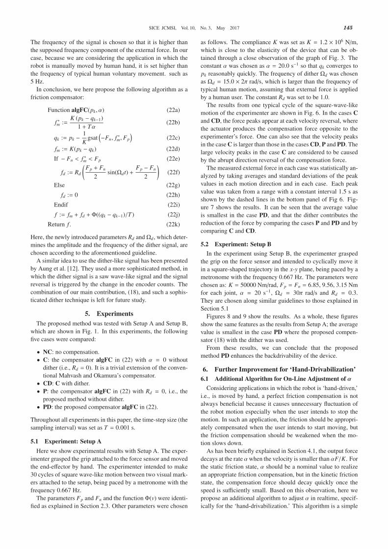
The results from one typical cycle of the square-wave-likemotion of the experimenter are shown in Fig. 6. In the cases Cand CD, the force peaks appear at each velocity reversal, wherethe actuator produces the compensation force opposite to theexperimenter’s force. One can also see that the velocity peaksin the case C is larger than those in the cases CD, P and PD. Thelarge velocity peaks in the case C are considered to be causedby the abrupt direction reversal of the compensation force.

The measured external force in each case was statistically an-alyzed by taking averages and standard deviations of the peakvalues in each motion direction and in each case. Each peakvalue was taken from a range with a constant interval 1.5 s asshown by the dashed lines in the bottom panel of Fig 6. Fig-ure 7 shows the results. It can be seen that the average valueis smallest in the case PD, and that the dither contributes thereduction of the force by comparing the cases P and PD and bycomparing C and CD.

5.2 Experiment: Setup B

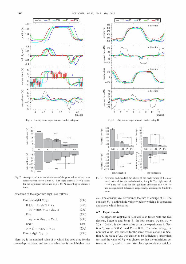
In the experiment using Setup B, the experimenter graspedthe grip on the force sensor and intended to cyclically move itin a square-shaped trajectory in the x-y plane, being paced by ametronome with the frequency 0.667 Hz. The parameters werechosen as: K = 50000 Nm/rad, Fp = Fn = 6.85, 9.56, 3.15 Nmfor each joint, α = 20 s−1, Ωd = 30π rad/s and Rd = 0.3.They are chosen along similar guidelines to those explained inSection 5.1

Figures 8 and 9 show the results. As a whole, these figuresshow the same features as the results from Setup A; the averagevalue is smallest in the case PD where the proposed compen-sator (18) with the dither was used.

From these results, we can conclude that the proposedmethod PD enhances the backdrivability of the device.

6. Further Improvement for ‘Hand-Drivabilization’6.1 Additional Algorithm for On-Line Adjustment of α

Considering applications in which the robot is ‘hand-driven,’i.e., is moved by hand, a perfect friction compensation is notalways beneficial because it causes unnecessary fluctuation ofthe robot motion especially when the user intends to stop themotion. In such an application, the friction should be appropri-ately compensated when the user intends to start moving, butthe friction compensation should be weakened when the mo-tion slows down.

As has been briefly explained in Section 4.1, the output forcedecays at the rate αwhen the velocity is smaller than αF/K. Forthe static friction state, α should be a nominal value to realizean appropriate friction compensation, but in the kinetic frictionstate, the compensation force should decay quickly once thespeed is sufficiently small. Based on this observation, here wepropose an additional algorithm to adjust α in realtime, specif-ically for the ‘hand-drivabilization.’ This algorithm is a simple

SICE JCMSI, Vol. 10, No. 3, May 2017146

Fig. 6 One cycle of experimental results, Setup A.

Fig. 7 Averages and standard deviations of the peak values of the mea-sured external force, Setup A. The triple asterisk (‘***’) standsfor the significant difference at p < 0.1 % according to Student’st-test.

extension of the algorithm algFC as follows:

Function algFC2(pk) (23a)

If |(pk − pk−1)/T | > VW (23b)

wk := max(wk−1 + RW , 1) (23c)

Else (23d)

wk := min(wk−1 − RW , 0) (23e)

Endif (23f)

α := (1 − wk)αN + wkαH (23g)

Return algFC(pk, α). (23h)

Here, αN is the nominal value of α, which has been used for thenon-adaptive cases, and αH is a value that is much higher than

Fig. 8 One part of experimental results, Setup B.

Fig. 9 Averages and standard deviations of the peak values of the mea-sured external force in each direction, Setup B. The triple asterisk(‘***’) and ‘ns’ stand for the significant difference at p < 0.1 %and no significant difference, respectively, according to Student’st-test.

αN . The constant RW determines the rate of change of α. Theconstant VW is a threshold velocity below which α is decreasedand above which increased.

6.2 Experiments

The algorithm algFC2 in (23) was also tested with the twodevices, Setup A and Setup B. In both setups, we set αN =

20 s−1 (which is the same value as in the experiments in Sec-tion 5), αH = 500 s−1 and RW = 0.01. The value of αN , thenominal value, was chosen for the same reason as for α in Sec-tion 5, the value of αH was chosen to be sufficiently larger thanαN , and the value of RW was chosen so that the transitions be-tween α = αN and α = αH take place appropriately quickly.

SICE JCMSI, Vol. 10, No. 3, May 2017 147

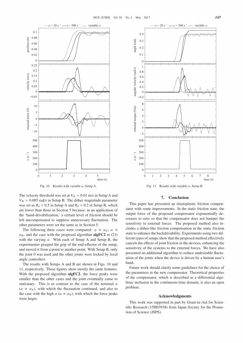
Fig. 10 Results with variable α, Setup A.

The velocity threshold was set at VW = 0.01 m/s in Setup A andVW = 0.005 rad/s in Setup B. The dither magnitude parameterwas set as Rd = 0.5 in Setup A and Rd = 0.2 in Setup B, whichare lower than those in Section 5 because, in an application ofthe ‘hand-drivabilization,’ a certain level of friction should beleft uncompensated to suppress unnecessary fluctuation. Theother parameters were set the same as in Section 5.

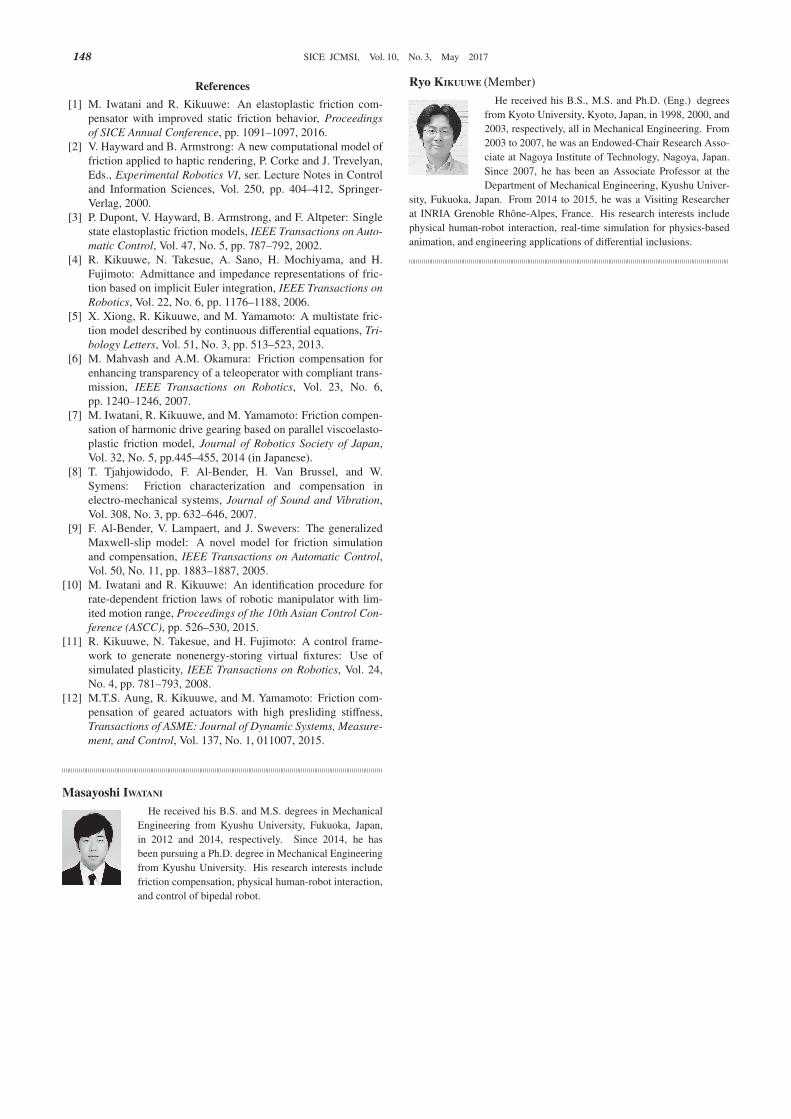
The following three cases were compared: α ≡ αN , α ≡αH , and the case with the proposed algorithm algFC2 in (23)with the varying α. With each of Setup A and Setup B, theexperimenter grasped the grip of the end-effector of the setup,and moved it from a point to another point. With Setup B, onlythe joint 0 was used and the other joints were locked by localangle controllers.

The results with Setups A and B are shown in Figs. 10 and11, respectively. These figures show mostly the same features.With the proposed algorithm algFC2, the force peaks weresmaller than the other cases and the joint eventually came tostationary. This is in contrast to the case of the nominal α(α ≡ αN), with which the fluctuation continued, and also tothe case with the high α (α ≡ αH), with which the force peakswere larger.

Fig. 11 Results with variable α, Setup B.

7. Conclusion

This paper has presented an elastoplastic friction compen-sator with some improvements. In the static friction state, theoutput force of the proposed compensator exponentially de-creases to zero so that the compensator does not hamper thesensitivity to external forces. The proposed method also in-cludes a dither-like friction compensation in the static frictionstate to enhance the backdrivability. Experiments using two dif-ferent types of setups show that the proposed method effectivelycancels the effects of joint friction in the devices, enhancing thesensitivity of the systems to the external forces. We have alsopresented an additional algorithm to reduce undesirable fluctu-ation of the joints when the device is driven by a human user’shand.

Future work should clarify some guidelines for the choice ofthe parameters in the new compensator. Theoretical propertiesof the compensator, which is described as a differential alge-braic inclusion in the continuous-time domain, is also an openproblem.

Acknowledgments

This work was supported in part by Grant-in-Aid for Scien-tific Research (15H03938) from Japan Society for the Promo-tion of Science (JSPS).

SICE JCMSI, Vol. 10, No. 3, May 2017148

References

[1] M. Iwatani and R. Kikuuwe: An elastoplastic friction com-pensator with improved static friction behavior, Proceedingsof SICE Annual Conference, pp. 1091–1097, 2016.

[2] V. Hayward and B. Armstrong: A new computational model offriction applied to haptic rendering, P. Corke and J. Trevelyan,Eds., Experimental Robotics VI, ser. Lecture Notes in Controland Information Sciences, Vol. 250, pp. 404–412, Springer-Verlag, 2000.

[3] P. Dupont, V. Hayward, B. Armstrong, and F. Altpeter: Singlestate elastoplastic friction models, IEEE Transactions on Auto-matic Control, Vol. 47, No. 5, pp. 787–792, 2002.

[4] R. Kikuuwe, N. Takesue, A. Sano, H. Mochiyama, and H.Fujimoto: Admittance and impedance representations of fric-tion based on implicit Euler integration, IEEE Transactions onRobotics, Vol. 22, No. 6, pp. 1176–1188, 2006.

[5] X. Xiong, R. Kikuuwe, and M. Yamamoto: A multistate fric-tion model described by continuous differential equations, Tri-bology Letters, Vol. 51, No. 3, pp. 513–523, 2013.

[6] M. Mahvash and A.M. Okamura: Friction compensation forenhancing transparency of a teleoperator with compliant trans-mission, IEEE Transactions on Robotics, Vol. 23, No. 6,pp. 1240–1246, 2007.

[7] M. Iwatani, R. Kikuuwe, and M. Yamamoto: Friction compen-sation of harmonic drive gearing based on parallel viscoelasto-plastic friction model, Journal of Robotics Society of Japan,Vol. 32, No. 5, pp.445–455, 2014 (in Japanese).

[8] T. Tjahjowidodo, F. Al-Bender, H. Van Brussel, and W.Symens: Friction characterization and compensation inelectro-mechanical systems, Journal of Sound and Vibration,Vol. 308, No. 3, pp. 632–646, 2007.

[9] F. Al-Bender, V. Lampaert, and J. Swevers: The generalizedMaxwell-slip model: A novel model for friction simulationand compensation, IEEE Transactions on Automatic Control,Vol. 50, No. 11, pp. 1883–1887, 2005.

[10] M. Iwatani and R. Kikuuwe: An identification procedure forrate-dependent friction laws of robotic manipulator with lim-ited motion range, Proceedings of the 10th Asian Control Con-ference (ASCC), pp. 526–530, 2015.

[11] R. Kikuuwe, N. Takesue, and H. Fujimoto: A control frame-work to generate nonenergy-storing virtual fixtures: Use ofsimulated plasticity, IEEE Transactions on Robotics, Vol. 24,No. 4, pp. 781–793, 2008.

[12] M.T.S. Aung, R. Kikuuwe, and M. Yamamoto: Friction com-pensation of geared actuators with high presliding stiffness,Transactions of ASME: Journal of Dynamic Systems, Measure-ment, and Control, Vol. 137, No. 1, 011007, 2015.

Masayoshi IWATANI

He received his B.S. and M.S. degrees in MechanicalEngineering from Kyushu University, Fukuoka, Japan,in 2012 and 2014, respectively. Since 2014, he hasbeen pursuing a Ph.D. degree in Mechanical Engineeringfrom Kyushu University. His research interests includefriction compensation, physical human-robot interaction,and control of bipedal robot.

Ryo KIKUUWE (Member)

He received his B.S., M.S. and Ph.D. (Eng.) degreesfrom Kyoto University, Kyoto, Japan, in 1998, 2000, and2003, respectively, all in Mechanical Engineering. From2003 to 2007, he was an Endowed-Chair Research Asso-ciate at Nagoya Institute of Technology, Nagoya, Japan.Since 2007, he has been an Associate Professor at theDepartment of Mechanical Engineering, Kyushu Univer-

sity, Fukuoka, Japan. From 2014 to 2015, he was a Visiting Researcherat INRIA Grenoble Rhone-Alpes, France. His research interests includephysical human-robot interaction, real-time simulation for physics-basedanimation, and engineering applications of differential inclusions.