This content has been downloaded from IOPscience. Please scroll down to see the full text.

Download details:

IP Address: 134.153.184.170

This content was downloaded on 27/06/2014 at 08:48

Please note that terms and conditions apply.

Some open problems of generalised Bessel polynomials

View the table of contents for this issue, or go to the journal homepage for more

1984 J. Phys. A: Math. Gen. 17 2759

(http://iopscience.iop.org/0305-4470/17/14/019)

Home Search Collections Journals About Contact us My IOPscience

J . Phys. A: Math. Gen. 17 (1984) 2759-2766. Printed in Great Britain

Some open problems of generalised Bessel polynomials

F Galvezt and J S Dehesae t Departamento de Fisica Tebrica, Facultad de Ciencias, Universidad de Granada, Granada, Spain $ Departamento de Fisica Nuclear, Facultad de Ciencias, Universidad de Granada, Granada, Spain

Received 29 March 1984

Abstract. The solution of several open problems connected with the generalised Bessel polynomials, which appear in solving the wave equation in spherical coordinates and in network synthesis and design, is shown. In particular, explicit and simple recursion formulae for sums of powers and product sums of the zeros of these polynomials are found. Also, three different sets of sums of generalised Bessel polynomials are analytically evaluated in a compact way.

1. Introduction

The Bessel polynomials appeared in the early thirties (Bochner 1929, Burchnall and Chaundy 1931) as the fourth class of orthogonal polynomials satisfying a second-order differential equation, the others being the classical systems of Jacobi, Laguerre and Hermite. However, the first systematic study of their properties was not done till twenty years later (Krall and Frink 1949) in connection with the solution of the wave equation in spherical coordinates. Shortly afterwards it was realised (Thomson 1949, 1952) the important role which these polynomials play in the theory of networks so that today they can be found not only in advanced articles (see e.g. Marshak et a1 1974, Johnson eta1 1976) but also in textbooks (Guillemin 1958, Hazony 1963, Weinberg 1975) of network synthesis and design. For more information and details about the Bessel polynomials and its applications see the excellent monograph (Grosswald 1978).

Here it is our purpose to show the solution of the following open problems of the Generalised Bessel Polynomials (GBP’S) y n ( x ; a, b) .

(i) To find explicit formulae for the Newton sums s, r = 1,2, . . . of y, (x ; a, b ) , that is for the rth power sum symmetric functions or just sums of rth powers of the zeros of the polynomial y, (x ; a, b ) .

(ii) To find simple recurrence relations for the sums s, ( i i i ) To obtain explicit expressions for the so-called homogeneous product sum

(iv) To derive new partial sums of GBP’S in an analytical way. The first two problems are explicitly pointed out by Grosswald (1978). They involve

the quantities s, which when conveniently normalised represent the moments about the origin of the distribution density of zeros of the polynomial y , ( x ; a, b) .

The structure of the paper is as follows. In 3 2 we briefly summarise the definition and the properties of the GBP’S which are needed for our discussion. The following

symmetric functions h, r = 1,2, . . . of the zeros of the polynomial y n ( x ; a, b ) .

0305-44701841142759 +08$02.25 0 1984 The Institute of Physics 2759

2760 F Galuez and J S Dehesa

section contains the solutions and proofs of the first two problems, that is those which involve the most useful and elementary sum rules of the zeros of the polynomial y , ( x ; a, b) . Section 4 is devoted to problem (iii), then to the more complicated sum rules of zeros h, Finally in 0 5 problem (iv) is considered. In particular three different sets of formulae for some partial sums of GBP'S are developed.

2. Review

The GBP y , ( x ; a, b ) was defined (Krall and Frink 1949) as the polynomial solution of the differential equation

x2-v"+( ax + b ) y ' - n ( n + a - 1)y = 0, b#O,a#O,- l , -2 , . . . . ( 1 )

Since y , (bx ; a, b ) is independent of b, it turns out that b is only a scale factor for the independent variable and not an essential parameter. This is why some authors prefer to use the polynomials y n ( x ; u ) = y n ( x ; a,2) or even Y ? ) ( x ) = y , , ( x ; a +2,2) so that y , , ( x ; 2) = Yio'(x) = y , ( x ) , the ordinary Bessel polynomial (Grosswald 1978, Chihara 1978).

The explicit expression of the GBP y , ( x ; a, 6) is (Grosswald 1978)

Here we have used the notation

u ( i ) = u ( u - l ) (u -2 ) . . . ( u - i + l ) , j2 1, U(')= 1.

In addition the GBP'S satisfy the three-term recursion relation (Krall and Frink 1949)

( n + a - 1)(2n + a - 2 ) y , + ,

= [ ( 2 n + a ) ( 2 n + a - 2 ) ( x / b ) + a - 2 ] ( 2 n +a- l )y ,

+n(2n + a ) y n - , , n 2 2 ,

with the initial conditions y o ( x ) = 1 and y l ( x ) = 1 + a ( x / b ) .

3. Sum rules of zeros s,

Let us denote by s, the sums of the rth power of the zeros { x I , x 2 , polynomial y , ( x ; a, b ) , i.e.

n

sr = c x:, r = 1 , 2 , . . . . " = I

The explicit expression of s, in terms of a and b turns out to be

(-1 +Zh) ! r fi ( (-b) 'n( ') s r = C(-l)r-Z'

( A ) A , ! h Z ! . . . h n ! I = I i ! (2n+a-2)")

, .

(3 )

, x n } of the

(4)

where Zh =.Cy=, hi, and the summation I;(') runs over all the partitions ( A , , h2, . . . , A,) of the number r so that Zy=, ihi = r.

Generalised Bessel polynomials 276 1

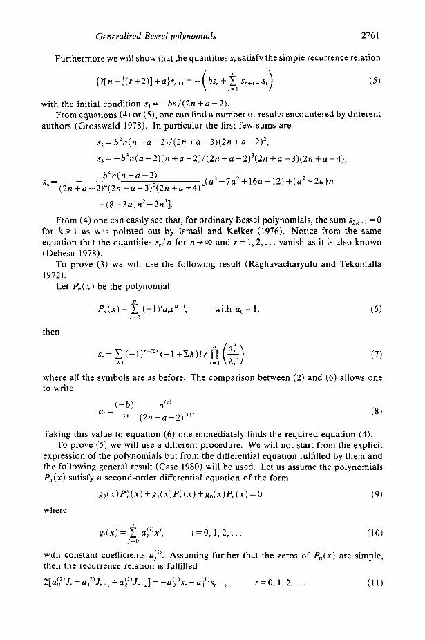
Furthermore we will show that the quantities s, satisfy the simple recurrence relation

with the initial condition s1 = -bn/(2n + a -2).

authors (Grosswald 1978). In particular the first few sums are From equations (4) or ( 5 ) , one can find a number of results encountered by different

s2 = b2n(n + a -2)/(2n + a -3)(2n + a -2)',

s3 = -b3n(a - 2 ) ( n + a -2)/(2n + a -2)3(2n + a -3)(2n + a -4),

b4n(n + a - 2 ) ( 2 n + ~ - 2 ) ~ ( 2 n + ~ - 3 ) ~ ( 2 n + a - 4 )

sq = [ (a3-7a2+16a- 12)+(a2-2a)n

+(8-3a)n2-2n3].

From (4) one can easily see that, for ordinary Bessel polynomials, the sum S2k+l = 0 for ks 1 as was pointed out by Ismail and Kelker (1976). Notice from the same equation that the quantities s,/ n for n + co and r = 1,2, . . . vanish as it is also known (Dehesa 1978).

To prove (3) we will use the following result (Raghavacharyulu and Tekumalla 1972).

Let P n ( x ) be the polynomial n

P n ( x ) = 1 (-l) iatxn-i , with a o = 1. I =o

then

s,= 1 (-l)r-'A(-l +ZA)!r fi ($) ( A ) i = I

(7)

where all the symbols are as before. The comparison between (2) and (6) allows one to write

Taking this value to equation (6) one immediately finds the required equation (4). To prove (5) we will use a different procedure. We will not start from the explicit

expression of the polynomials but from the differential equation fulfilled by them and the following general result (Case 1980) will be used. Let us assume the polynomials P , , ( x ) satisfy a second-order differential equation of the form

( 9 ) g * ( x ) P X x ) + g l ( x ) P ' , ( x ) + g o ( x ) P n ( x ) = 0

where I

g A x ) = c a;')?, i = O , 1,2, . . . (10) J = o

with constant coefficients a;f). Assuming further that the zeros of P n ( x ) are simple, then the recurrence relation is fulfilled

( 1 1 ) 2[Ub*'J, +aj29,+, +a:2)J,+2] = -aY)s, - a(ll)s,+I, r = 0, 1,2, . . .

2762 F Galvez and J S Dehesa

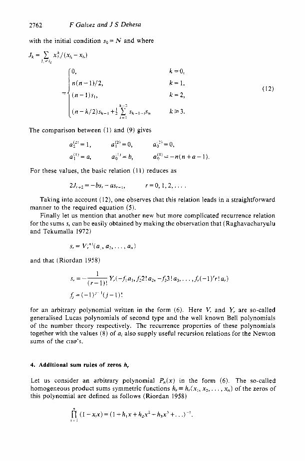
with the initial condition so= N and where

Jk = 1 x : / ( x l , - x / 2 ) / I f I2

k = 0 ,

k = 1,

k = 2,

The comparison between (1 ) and (9) gives

For these values, the basic relation (1 1 ) reduces as

2J,+, = -bs, - as,+I, r = 0 , 1,2,

Taking into account (12), one observes that this relation leads in a straightforward manner to the required equation (5).

Finally let us mention that another new but more complicated recurrence relation for the sums s, can be easily obtained by making the observation that (Raghavacharyulu and Tekumalla 1972)

s, = V;")(al, a,, . . . , a,)

and that (Riordan 1958)

for an arbitrary polynomial written in the form (6). Here V, and Y, are so-called generalised Lucas polynomials of second type and the well known Bell polynomials of the number theory respectively. The recurrence properties of these polynomials together with the values (8) of ai also supply useful recursion relations for the Newton sums of the GBP'S.

4. Additional sum rules of zeros h,

Let us consider an arbitrary polynomial P n ( x ) in the form ( 6 ) . The so-called homogeneous product sums symmetric functions h, = h , ( x , , x2 , . . . , x , ) of the zeros of this polynomial are defined as follows (Riordan 1958)

Generalised Bessel polynomials 2763

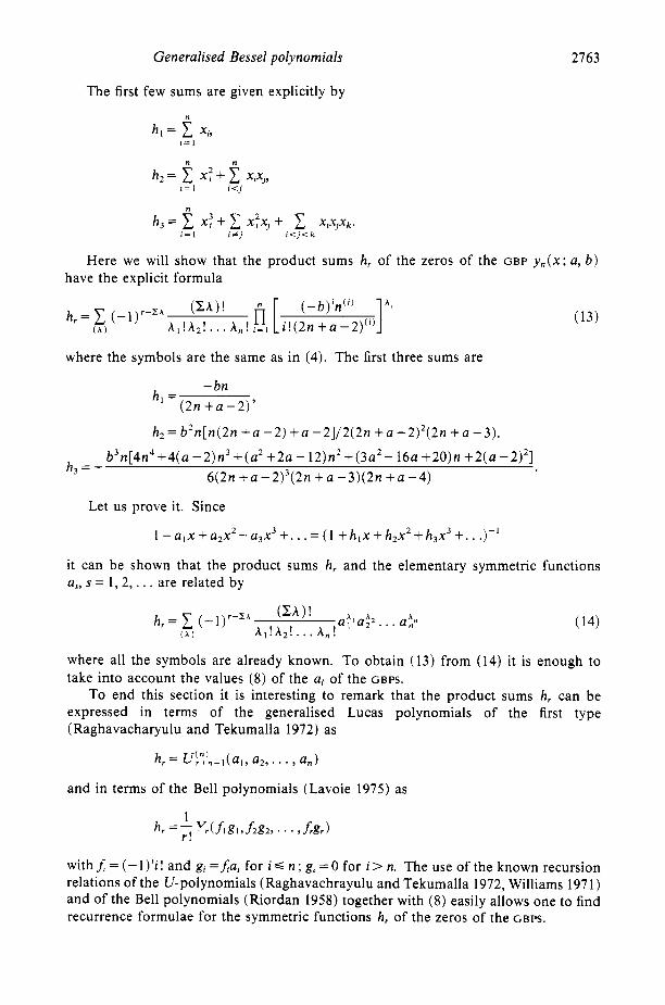
The first few sums are given explicitly by n

h l = C Xir i - I

n n h2 = C x ; + C xixj,

, = I i < j

h3 = X : + X : X , x,xjxk. i = l i # j i c j < k

Here we will show that the product sums hr of the zeros of the GBP y , ( x ; a, b) have the explicit formula

where the symbols are the same as in (4). The first three sums are

-bn (2n + a - 2 ) '

h , =

h 2 = b2n[n(2n + a -2) + a -2]/2(2n + a -2)2(2n + a -3).

b3n[4n4+4(a-2)n3 + ( a 2 +2a - 12)n2+(3a2- 16a +20)n +2(a -2)*] 6(2n + a -2)3(2n + a -3)(2n + a -4)

h 3 = -

Let us prove it. Since

1 - U ~ X + a , x 2 - a 3 x 3 +. , .=( 1 + h1x + h2x2+ h3x3 +. . . ) - I

it can be shown that the product sums h, and the elementary symmetric functions a,, s = 1,2, . . . are related by

where all the symbols are already known. To obtain (13) from (14) it is enough to take into account the values (8) of the ai of the GBPS.

To end this section it is interesting to remark that the product sums h, can be expressed in terms of the generalised Lucas polynomials of the first type (Raghavacharyulu and Tekumalla 1972) as

h r = U!"?,-l(al, ~ 2 9 . . ., an)

and in terms of the Bell polynomials (Lavoie 1975) as

1 hr =A vr(flgl,f*gz,~. . , f , g r )

with 1; = (- 1 ) j i ! and gi =Lai for i S n ; g, = 0 for i > n. The use of the known recursion relations of the U-polynomials (Raghavachrayulu and Tekumalla 1972, Williams 197 1) and of the Bell polynomials (Riordan 1958) together with (8) easily allows one to find recurrence formulae for the symmetric functions hr of the zeros of the GBPS.

2164 F Galvez and J S Dehesa

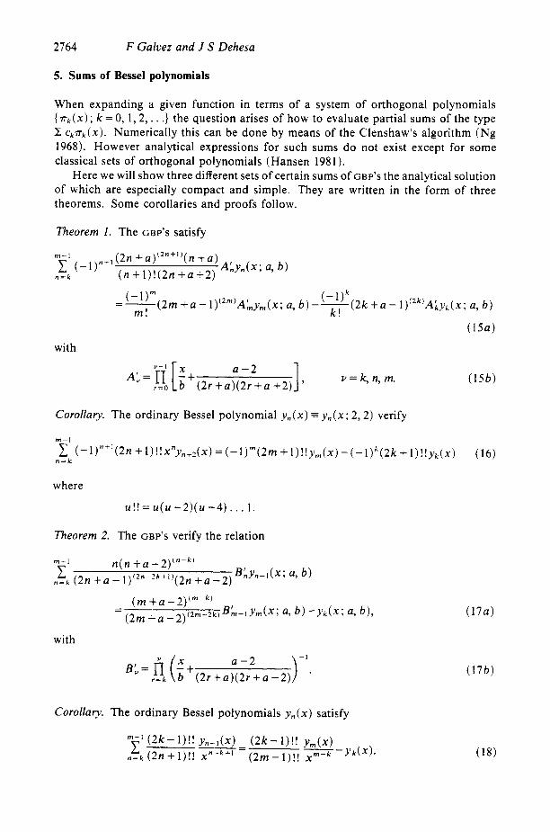
5. Sums of Bessel polynomials

When expanding a given function in terms of a system of orthogonal polynomials {vk(X); k = 0, 1,2, . . .} the question arises of how to evaluate partial sums of the type C ck7rk(x). Numerically this can be done by means of the Clenshaw's algorithm (Ng 1968). However analytical expressions for such sums do not exist except for some classical sets of orthogonal polynomials (Hansen 198 1 ).

Here we will show three different sets of certain sums of GBP'S the analytical solution of which are especially compact and simple. They are written in the form of three theorems. Some corollaries and proofs follow.

Theorem 1. The GBP'S satisfy

m-1 (2n + n + a ) n = k ( n +1)!(2n + a +2) c ( - l ) n + l A',yn(x; a, b )

-- - (-')m(2m + a - l)""A&y,(x; a, b ) - O ' ( 2 k + a - 1)'2k'A'kyk(x; a, b ) m ! k!

with

v = k, n, m. ( 2 r + a ) ( 2 r + a + 2 ) a - 2 1 '

Corollary. The ordinary Bessel polynomial y,, (x) = y , (x ; 2,2) verify

where

U !! = U( U - 2)( U - 4) . , . 1

Theorem 2. The GBP'S verify the relation

with

Corollary. The ordinary Bessel polynomials y , (x) satisfy

Generalised Bessel polynomials 2765

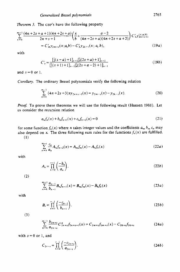
Theorem 3. The GBP’S have the following property

( x : a , b ) C;Ylfl+s+l

( 1 9 a )

m - l ( 4 n +2s + a + 1)(4n +2s + a ) x a - 2 n = k c 2n+s+1 ( i ;+ (4n+2s+a) (4n+2s+a+2)

= CLY2m+s(X;a,b)- C;YZk+s(X; a, b ) ,

with

[ j (s + a ) + 1]”-l[:(2s + a ) + 1 I y - l

[& + 1 ) + 1],-,[:(2s + a - 2 ) + 1 ] , - I CL=

and s - 0 or 1.

Corollary. The ordinary Bessel polynomials verify the following relation

n = k

Roo$ To prove these theorems we will use the following result (Hansen 1981). Let us consider the recursion relation

for some function f n ( x ) where n takes integer values and the coefficients a,, b,, e, may ollowing sum rules for the functions f , ( x ) are fulfilled. also depend on x. The three

( 1 )

with r - l

A,= n (2). n = O

with

with s = O or 1, and

2766 F Galvez and J S Dehesa

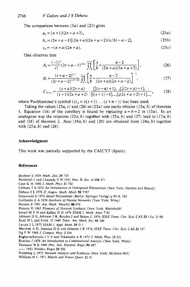
The comparison between ( 3 a ) and (21) gives

a, = (n + 1)(2n + a +2),

6 , = ( 2 n + a + 1 ) [ ( 2 n + a ) ( 2 n + a + 2 ) ( x / b ) + a - 2 ] ,

c, = - (n +a) (2n + a ) .

One observes that

A, = -(2r + a - l ) (2r ) r!

a - 2 I-’ €3, = (2n+a)(2n + a - 2 ) ’

(28) ( s + a ) ( 2 s + a ) [ f ( s + a ) + l ] T - , [ ~ ( 2 S + a ) + l ] , _ ’

(s + 1)(2s + a +2) [$(s + 1 ) + 1],-,[$(2s + a +2) + l ] r - ’y C 2 r + r =

where Pochhammer’s symbol ( z ) , = z(z + 1) . . . (z + n - 1 ) has been used. Taking the values (25a, c ) and (26) to (22a) one easily obtains (1.5~’ b) of theorem

1. Equation (16) of the corollary is found by replacing a = b = 2 in ( 1 5 ~ ) . In an analogous way the relations (23a, b) together with (25~1, b ) and (27) lead to (17~1, b ) and (18) of theorem 2. Also (19~1, b) and (20) are obtained from (24a, b) together with (25a, b ) and (28).

Acknowledgment

This work was partially supported by the CAICYT (Spain).

References

Bochner S 1929 Math. Zeit. 29 730 Burchnall J and Chaundy T W 1931 h o c . R. Soc. A 134 471 Case K M 1980 J. Math. Phys. 21 702 Chihara T S 1978 An Introduction to Orthogonal Polynomials (New York: Gordon and Breach) Dehesa J S 1978 Z. Angew. Math. Mech. 58 T397 Grosswald E 1978 Bessel Polynomials (Berlin: Springer Verlag) p 93-8, 163 Guillemin E A 1958 Synthesis ofPassioe Networks (New York: Wiley) Hansen E 1981 Am. Math. Monthly 88 676 Hazony D 1963 Elements of Network Synthesis (New York: Rheinhold) Ismail M E H and Kelker D H 1976 SIAM J. Math. Anal. 7 82 Johnson D E, Johnson J R, Boudra J and Stokes C 1976 IEEE Trans. Circ. Syst. CAS 23 (No. 2) 96 G a l l H L and Frink 0 1949 Trans. Am. Math. Soc. 65 100 Lavoie J L 1975 SIAM J. Appl. Math. 29 51 1 Marshak A H, Johnson D E and Johnson J R 1974 IEEE Trans. Circ. Syst. CAS 21 797 Ng E W 1968 J. Comput. Phys. 3 334 Raghavacharyulu I V V and Tekumalla A R 1972 J. Math. Phys. 13 321 Riordan J 1958 An Introduction to Combinatorial Analysis (New York: Wiley) Thomson W E 1949 Proc. Inst. Electron. Engrs 96 487 - 1952 Wireless Engrs 29 256 Weinberg L 1975 Network Analysis and Synthesis (New York: McGraw-Hill) Williams H C 1971 Matrix and Tensor @art. 21 91