Embed Size (px)
Citation preview
i
Some selected Topics in Geometric Functions Theory of a Complex Variable
DOCTOR OF PHILOSPHY IN MATHEMATICS
By
Ali Muhammad
Department of Mathematics
COMSATS Institute of Information Technology
Islamabad – Pakistan
January 2009
ii
COMSATS Institute of Information Technology, Islamabad-Pakistan
A thesis presented to COMSATS Institute of Information Technology,
Islamabad In partial fulfilment
of the requirement for the degree of
DOCTOR OF PHILOSPHY IN MATHEMATICS
By
Ali Muhammad
CIIT/FA05-PMT-002/ISB
iii
Some selected Topics in Geometric Functions Theory of a Complex Variable
A Post Graduate thesis submitted to the Department of Mathematics
As partial fulfilment for the award of Degree DOCTOR OF PHILOSPHY IN MATHEMATICS
Name Registration Number Ali Muhammad CIIT/FA05-PMT-002/ISB
Supervisor: Dr. Khalida Inayat Noor Professor Department of Mathematics CIIT, Islamabad
Signature ________
Ali Muhammad CIIT/FA05-PMT-002/ISB
COMSATS Institute of Information Technology, Islamabad
iv
Final Approval
This thesis titled Some selected Topics in Geometric Functions
Theory of a Complex Variable
submitted for the degree of
DOCTOR OF PHILOSPHY IN MATHEMATICS By
Ali Muhammad
CIIT/FA05-PMT-002/ISB
has been approved for COMSATS Institute of Information Technology, Islamabad
External Examiner: __________________________ Dr Ikram A. Tirmizi Professor of Mathematics GIK, Institute of Engineering and Technology, Topi(N.W.F.P)Pakistan
Supervisor : __________________________ Dr. Khalida Inayat Noor Professor of Mathematics CIIT, Islamabad
Head Department of : __________________________ Mathematics Dr. Saleem Asghar Professor of Mathematics
CIIT, Islamabad
Dean :__________________________ Dr. Raheel Qamar Faculty of Sciences
CIIT, Islamabad
v
Certificate
I hereby declare that this project neither as a whole nor as a part there of has been copied out from any source. It is further declared that I have developed this thesis and the accompanied report entirely on the basis of my personal efforts made under the sincere guidance of my supervisor. No portion of the work presented in this thesis has been submitted in support of any other degree or qualification of this or any other University or Institute of learning, if found I shall stand responsible.
Signature:_______________
Name: Ali Muhammad Registration No: CIIT/FA05-PMT-002/ISB

vi
Dedicated to
my parents my wife
and my loveing daughter Alina.
vii
Acknowledgements
All Praises belong to Almighty Allah, Lord and the Creator of the universe Who
bestowed upon me the courage and His countless blessing enabled me to accomplish
my Ph.D. Studies. He is the Most Powerful, Gracious and Beneficent. All respect to
our Holy prophet Muhammad (peace be upon him) who enables us to recognize our
creator Allah, and who is forever a torch of guidance for the whole mankind.
My heartiest profound gratitude is to my respected and worthy supervisor Professor
Dr Khalida Inayat Noor for her invaluable and inspiring guidance and encouraging
discussions which enabled me to complete my work successfully. Her encouraging
and instructive behaviour always motivated me to implement new ideas in my
research work. My Allah blesses her with her best. Infact it is a matter of pride and
privilege for me to be her Ph.D. student.
Thanks are also due to my chairman, Professor Dr Saleem Asghar Department of
Mathematics COMSATS Institute of Information Technology for providing necessary
research facilities.
I am highly indebted to my respectable teacher Professor Dr Muhammad Aslam
Noor for his guidance during my course work. I express deep gratitude to Dr S. M.
Junaid Zaidi, Rector, CIIT, for his support and providing excellent research
facilities. I gratefully thank to COMSATS Institute of Information Technology for
providing financial help in the form of scholarships to undertake my Ph.D. studies
I have a strong feeling of appreciation, for Higher Education Commission of
Pakistan for providing the latest literature and research materials in the form of the
updated digital and reference libraries. I am proud of my friends and colleagues Mr.
Saqib Hussain, Mr. Muhammad Arif, Mr. Waseem ul Haq and Mr Waseem Asghar
khan for their valuable discussions during my research work.
At the end, this arduous task would have been really difficult without the prayers and
wishes of my parents and other member of my family. Especially, I owe gratitude to
my mother and wife.
Ali Muhammad
viii
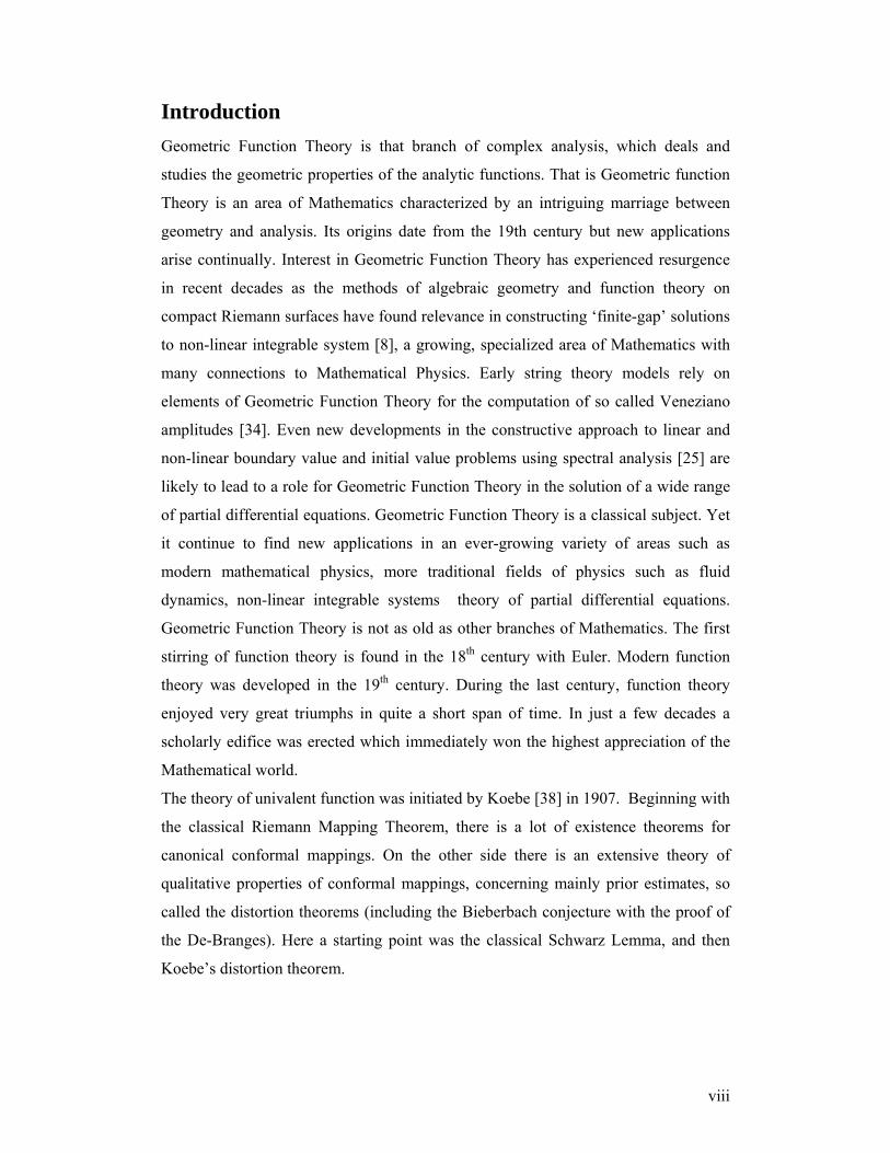
Introduction Geometric Function Theory is that branch of complex analysis, which deals and
studies the geometric properties of the analytic functions. That is Geometric function
Theory is an area of Mathematics characterized by an intriguing marriage between
geometry and analysis. Its origins date from the 19th century but new applications
arise continually. Interest in Geometric Function Theory has experienced resurgence
in recent decades as the methods of algebraic geometry and function theory on
compact Riemann surfaces have found relevance in constructing ‘finite-gap’ solutions
to non-linear integrable system [8], a growing, specialized area of Mathematics with
many connections to Mathematical Physics. Early string theory models rely on
elements of Geometric Function Theory for the computation of so called Veneziano
amplitudes [34]. Even new developments in the constructive approach to linear and
non-linear boundary value and initial value problems using spectral analysis [25] are
likely to lead to a role for Geometric Function Theory in the solution of a wide range
of partial differential equations. Geometric Function Theory is a classical subject. Yet
it continue to find new applications in an ever-growing variety of areas such as
modern mathematical physics, more traditional fields of physics such as fluid
dynamics, non-linear integrable systems theory of partial differential equations.
Geometric Function Theory is not as old as other branches of Mathematics. The first
stirring of function theory is found in the 18th century with Euler. Modern function
theory was developed in the 19th century. During the last century, function theory
enjoyed very great triumphs in quite a short span of time. In just a few decades a
scholarly edifice was erected which immediately won the highest appreciation of the
Mathematical world.
The theory of univalent function was initiated by Koebe [38] in 1907. Beginning with
the classical Riemann Mapping Theorem, there is a lot of existence theorems for
canonical conformal mappings. On the other side there is an extensive theory of
qualitative properties of conformal mappings, concerning mainly prior estimates, so
called the distortion theorems (including the Bieberbach conjecture with the proof of
the De-Branges). Here a starting point was the classical Schwarz Lemma, and then
Koebe’s distortion theorem.
ix
The theory of univalent functions is one of the most beautiful subjects in Geometric
Function Theory. Its origin (apart from the Riemann mapping Theorem) can be traced
to the 1907 paper of Koebe [38], to Gronwall’s proof of the Area Theorem in 1914
and to Bieberbach’s estimate for the second coefficient of normalized univalent
functions in 1916 and its consequences. By then, univalent function theory was a
subject in its own right.
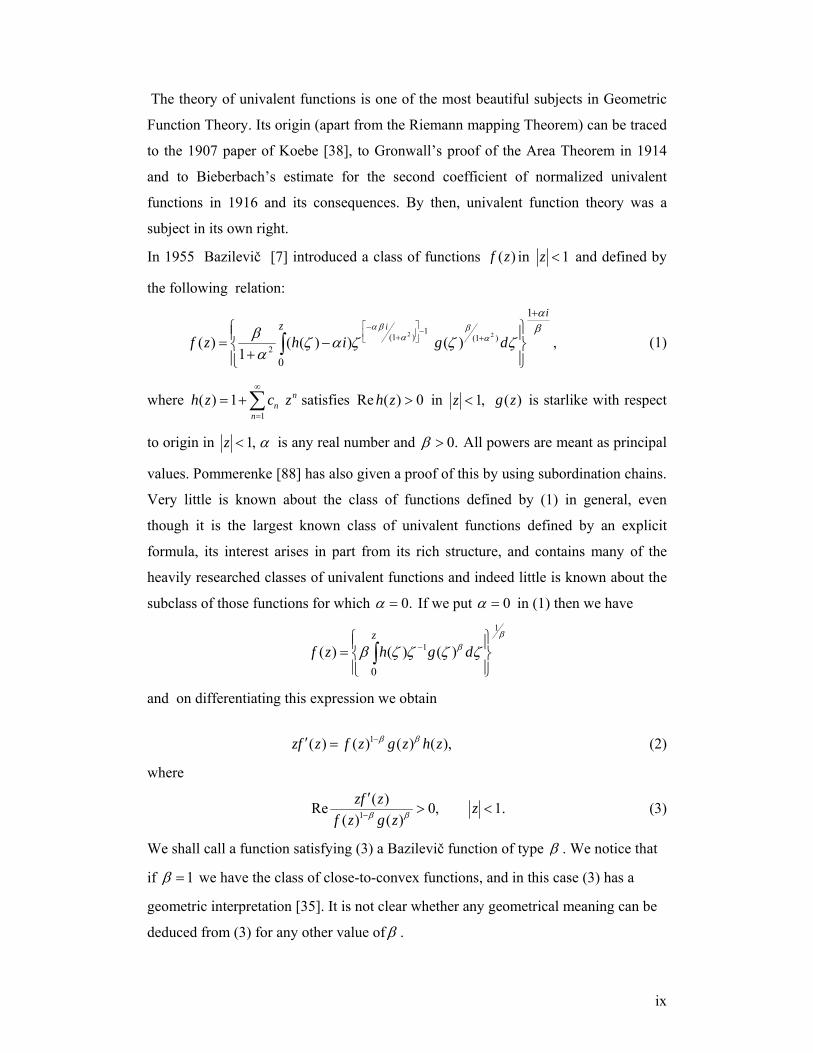
In 1955 Bazilevič [7] introduced a class of functions ( )f z in 1z < and defined by
the following relation:
2 21(1 ) (1 )
2
1
0
( ) ( ( ) ) ( ) ,1
ii
zf z h i g d
α β βα α
αββ ζ α ζ ζ ζ
α
⎡ ⎤− −⎢ ⎥+ +⎣ ⎦
+⎧ ⎫⎪ ⎪= −⎨ ⎬+⎪ ⎪⎩ ⎭
∫ (1)
where 1
( ) 1 nn
nh z c z
∞
=
= +∑ satisfies Re ( ) 0h z > in 1,z < ( )g z is starlike with respect
to origin in 1,z < α is any real number and 0.β > All powers are meant as principal
values. Pommerenke [88] has also given a proof of this by using subordination chains.
Very little is known about the class of functions defined by (1) in general, even
though it is the largest known class of univalent functions defined by an explicit
formula, its interest arises in part from its rich structure, and contains many of the
heavily researched classes of univalent functions and indeed little is known about the
subclass of those functions for which 0.α = If we put 0α = in (1) then we have 1
1
0
( ) ( ) ( )z
f z h g dβ
ββ ζ ζ ζ ζ−⎧ ⎫⎪ ⎪= ⎨ ⎬⎪ ⎪⎩ ⎭∫
and on differentiating this expression we obtain
1( ) ( ) ( ) ( ),zf z f z g z h zβ β−′ = (2)
where
1
( )Re 0, 1.( ) ( )
zf z zf z g zβ β−
′> < (3)
We shall call a function satisfying (3) a Bazilevič function of type β . We notice that
if 1β = we have the class of close-to-convex functions, and in this case (3) has a
geometric interpretation [35]. It is not clear whether any geometrical meaning can be
deduced from (3) for any other value ofβ .
x
The Bieberbach conjecture is still unsettled for Bazilevič functions, the only
contribution so far being made by J. Zamorski [123] who showed that the conjecture
is valid when 1Nβ = , N being a positive integer. In 1968 Thomas [114] asked if it
was possible to give a geometric characterization of the Bazilevič functions when
0.α = He then proved that the Taylor coefficients of bounded Bazilevic functions
when 0α = satisfy 1na O
n⎛ ⎞= ⎜ ⎟⎝ ⎠
which extended Clunie and Pommerenke’s result
[19] for bounded close-to-convex functions.
In 1971 Sheil-Small [101] gave an intrinsic characterization for the ordinary Bazilevič
functions along the lines of Kaplan’s characterization of the close-to-convex functions
[35]. He proved each ordinary Bazilevic function ( )f z is a solution of the differential
equation
( ) ( ) ( ) ( )1 ( 1 )( ) ( ) ( ) ( )
zf z zf z g z zh zi z if z f z g z h z
α β α β′ ′ ′ ′
+ + − + = + + (4)
g and h as before and extended the class to include the case 0.α = He gave the first
example (albeit non-constructive) of a non- Bazilevič univalent function.
In 1972 Prokhorov [92] characterized Bazilevič function of type α in terms of the
geometry of the complement of ( )f D as Lewandowski [40,41] had done for the
close-to-convex functions. In 1974 Avhadiev and Aksent’ev [6] completed this
program by characterizing Bazilevic functions of type ( , )α β in terms of the
complement of ( ).f D
The notion of the class of non- Bazilevič functions ( )N α was first introduced by
Obradovic [78] in 1998. Until now, the class of non- Bazilevič functions was studied
in a direction of finding necessary conditions over α that embeds this class into the
class of univalent functions or its subclass. In recent year a large number of papers
have appeared in the literature concerned with extending the results contained in
Obradovic’s paper [78]. Tuneski and Darus [115] obtained Fekete-Szego inequality
for the class of non-Bazilevic functions. Using the concept of non- Bazilevič class,
Wang et al [120] studied many subordination results for the generalized class of non-
Bazilevič functions.
It is well known [28] that a number of important classes of univalent functions (e.g.
convex, starlike) are related through their derivatives by functions with positive real
xi
part. These functions play an important part in problem from signal theory, in moment
problems and in constructing quadrature formulas, see Ronning [97] and the
references cited therein for some recent applications. In this thesis, we introduce and
consider some new classes of functions by replacing functions with positive real part
by certain weighted differences of such functions.
In chapter 1, we give preliminaries of Geometric Function Theory which are used in
the subsequent chapters, and we also study the classes of Bazilevič and non- Bazilevič
functions which are the main focus of our thesis.
In chapter 2, we define a new class В ( , )k α β for realα , 1 1,2
β−≤ <
2 and .k z E≥ ∈ The contents of this chapter have been published in the journal of
Applied Mathematics and Computations, see [76]. For different choices of parameters
,k α and β we presents its relationships with the previously known classes. It is
well known [113] 2В ( , )α β is a subclass of Bazilevic functions defined in [7], and
consists entirely of univalent functions. We study the relationship between the classes
В ( , )k α β and kR , where kR denotes the class of bounded radius rotation, see [36]. In
this chapter we also focus on the inclusion results between the classes В ( , )k α β and
1 1В ( , ).k α β We also establish the criterion of univalance for the class ( , )kB α β when
the value of 2( 2 1) , 0.(1 )
k α αβ β αβ
+ − +≤ ≠
− As a special case, we deduce that
2В ( , )f α β∈ is univalent in 1for 0, 1.2
E α β−> ≤ < Further we derive arc
lengths problems for the class В ( , )k α β and as a consequence of it we establish the
growth of the coefficient for the class В ( , )k α β by specializing the parameter 0.α >
The behavior of Barnardi integral operator in the class В (0, )k β is investigated. By
using the concept of Gauss hypergeometric function we have discussed in details the
sharp bounds of the class 2В ( , )α β for 0α ≠ and 0 1.β< < Finally, in this chapter,
for different parameters of interest we obtained the coefficient bounds by assuming
2a to be real. We also derive a covering and distortion theorems for the classes
2В ( , )α β and В (1, )k β by restricting the parameters ,k α and β .
xii
In chapter 3, we define the new class ,,В ( , , , ),p a c A Bλ μα where 0, 0, pμ α λ> ≥ > −
1 1, ,B A B A− ≤ ≤ ≠ ∈ and 0, \ {0, 1, 2, 3,...}a c −∈ = − − − of analytic functions
by using the method of differential subordination. The fascinating theory of
differential subordination was put on sound footing by Miller and Mocanu [58] in
1981. The class ,, ( , , , )pB a c A Bλ μα stem essentially from the class of Bazilevič functions.
After the appearance of [45], [78] and [103], several authors [91,121] have further
explored the properties of 0,1,В ( ,1, ,0)p Aμα and 0,
,1В ( ,1, , ), 1 1.p p A B B A Bμ − ≤ < ≤ <
Large number of known results also follows as particular cases from our results [45,
79, 91, 103,121]. We investigate a number of inclusion relationships for the class ,,В ( , , , ).p a c A Bλ μα We also focus on some interesting properties of the subclass
,1,В ( , , , ).p a c A Bλα The most interesting one is that the class ,1
,В ( , , , )p a c A Bλα is closed
under convolution convex function and the generalized Livingston-Libra-Bernardi
operator defined by (1.5.5), [43] belongs to this class. At the end of this chapter, we
establish distortion theorems for the class ,,В ( , , , )p a c A Bλ μα , the lower and upper
bounds of μλ
⎟⎟⎠
⎞⎜⎜⎝
⎛p
p
zzfcaI )(),(
Re for ,,( ) В ( , , , ),pf z a c A Bλ μα∈ and some other interesting
properties of p-valent functions which are defined here by means of a certain linear
operator ( , ) ( ).pI a c f zλ
Chapter 4 is mainly concerned with the class of p-valent non-Bazilevic functions ,, ( , , , )pN a c A Bλ μα where, 0 1,μ< < ,α ∈ 1 1, , ,B A B A− ≤ ≤ ≠ ∈ pλ > − ,
{1,2,3,...}p∈ = and 0, \ {0, 1, 2, 3,...}.a c −∈ = − − − of analytic functions. This
class generalizes the class of non- Bazilevič functions. The class of non- Bazilevič
functions was first introduced by Obradovic [78] in 1998. In this chapter, we are
primarily concerned with presenting some generalization and applications of the class
of p-valent non- Bazilevič functions. Large number of known results also follows as
particular cases from our results; see [78, 115, 118]. We establish a number of
inclusion relationships for the class ,, ( , , , ).pN a c A Bλ μα We derive distortion theorems
for the class ,, ( , , , )pN a c A Bλ μα , the lower and upper bounds of
μ
λ ⎟⎟⎠
⎞⎜⎜⎝
⎛
)(),(Re
zfcaIz
p
p
for
xiii
,,( ) ( , , , ),pf z N a c A Bλ μα∈ and some other interesting properties of p-valent functions
which are defined here by means of a certain linear integral operator ( , ) ( ).pI a c f zλ
Finally in this chapter, we derive an interesting sharp radius problem for the class ,, ( , , ).pN a cλ μα ρ
Chapter 5, is composed of two types of problems. The first type is concerned with
p-valent functions and the second type is concerned with meromorphic functions.
Making use of the generalized hypergeometric functions, we introduce certain new
subclass 1( , , , , , )kT p q sλ α ρ of p-valent analytic functions defined by Dziok-
Srivastava operator in the unit disc E . Many interesting subclasses of analytic
functions, associated with the Dziok−Srivastava operator , , 1( )p q sH α and its many
special cases, were investigated recently by Dziok and Srivastava [22,23],
Gangadharan et al [26], Liu [46], Liu and Srivastava [48], see also [46, 80,106]. In
part first of this chapter we obtain a number of new applications for this class of
p-valent functions. We investigate a number of inclusion relationships and derive a
sharp radius for the class 1( , , , , , )kT p q sλ α ρ . We prove that the class
1( , , , , , )kT p q sλ α ρ is closed under Hadamard product and we also investigate some
other interesting properties of p-valent functions which are defined here by means of a
certain linear integral operator , , 1( ).p q sH α
In the second part of this chapter, we also investigate the various important properties
and characteristics of the classes ( , , , , )kMB q sα λ ρ and ( , , , , ).kMT q sα λ ρ We define
two new subclasses, ( , , , , )kMB q sα λ ρ and ( , , , , )kMT q sα λ ρ of meromorphic
functions defined by using a meromorphic analogue of the Choi−Saigo−Srivastava
operator for the generalized hypergeometric function in the punctured unit disk .E ∗
Meromorphic functions have been extensively studied by for example Mogra [61, 62],
Uralegaddi and Ganigi [116], Uralegaddi and Somanatha [117], Aouf [3, 4],
Srivastava et al [109], Owa et al [81], Joshi and Aouf [32], Joshi and Srivastava [33],
Aouf et al [5], Raina and Srivastava [93] and Yang [122].
We derive several inclusion relationships for these function classes ( , , , , )kMB q sα λ ρ
and ( , , , , ).kMT q sα λ ρ We prove sharp radius theorem and we investigate the
integral preserving property for the class ( , , , , ).kMB q sα λ ρ At the end of this chapter,

xiv
we have shown that the two function classes ( , , , , )kMB q sα λ ρ and ( , , , , )kMT q sα λ ρ
are closed under convolutions. All the results obtained in this chapter are new .
xv
List of symbols A Class of normalized analytic functions in the open unit
disk E
( )pA Class of normalized P-valent functions in the open unit disk E
( , , , )B p gα β Class of Bazilevic functions of type α and order β
Complex plane C Class of convex functions
( )C ρ Class of convex functions of order ρ D Domain
1n pD + − Ruscheweyh derivative of ( 1)n p th+ − order E Open unit disk
* \{0}E E= Punctured unit disk
( , ; ; )G a b c z Gauss Hypergeometric functions
1 1( ,..., ; ,..., ; )q s q sF zα α β β Generealized Hypergeometric functions
, pδF Generalized Libra- Livingston-Barnardi operator
( )E=H H Class of analytic functions in the unit disk E
[ ],a nH Class of normalized analytic function in E
, , 1( )p q sH α Dziok - Srivastava operator
, , 1( )q sHλ α Choi-Saigo-Srivastava opearotor
H + Right half plan
1n pI + − Noor integral operator
( , )pI a cλ The Cho-Kown-Srivastava operator K Class of close-to-convex functions
xvi
( )K ρ Class of close-to-convex functions of order ρ
( )k z Koebe function
( , )p a cL Saitoh operator M Class of meromorphic functions Mα Class of alpha- convex functions
( )kM α Class of functions with bounded Mocanu variation
( )N α Class of non-Bazilevic functions Ρ Class of functions with positive real part
( ),Ρ ρ Class of functions with positive real part greater than
(0 1).ρ ρ≤ <
( )kΡ ρ Generalization of the class Ρ where (0 1)ρ ρ≤ <
and 2.k ≥
[ , ]A BΡ Class of Janowski’s function
kR Class of functions of bounded radius rotation
( )kR ρ Class of functions of bounded radius rotation of order
(0 1)ρ ρ≤ <
Sγ Class of spiral-like-functions
S∗ Class of starlike functions
( )S ρ∗ Class of starlike functions of order ρ
kV Class of functions of bounded radius rotations
( )kV ρ Class of functions of bounded radius rotation of order
ρ
)k(ν Pochhammer symbol
[ , ]n qΨ Ω Class of admissible functions
Φ Convolution operator
f g∗ Convolution of f and g
≺ Subordination
xvii
≺f g Subordination of f by g
xviii
Contents Introduction
Chapter 1 Some preliminary concepts of Geometric Function
Theory of a complex variable 1
1.1 Introduction 1 1.2 Basic definitions and some properties of the class of univalent functions 2
1.3 The class Ρ of functions with positive real part and some of its related 5
classes
1.3.1 The class Ρ 5
1.3.2 The class ( )Ρ ρ
1.3.3 The class [ , ]A BΡ 7 1.3.4 The class ( )kΡ ρ 9 1.4 Some classes of analytic functions 10
1.4.1 The class of starlike and Convex Functions 10
1.4.2 The class of alpha –convex functions 12
1.4.3 The class K of close-to-convex functions [21, 26]. 12
1.4.4 The class kV of functions with bounded boundary rotation 14
1.4.5 The class kR of functions with bounded radius rotation 16
xix
1.4.6 The class ( )kR ρ 16
1.4.7 The class ( )kV ρ 17
1.4.8 The class of Bazilevic functions 17
1.4.9 The class of Non-Bazilevic functions 18
1.5 P-valent functions and certain differential and integral operators 19
1.5.1 Hypergeometric function and
Hadamard product (or Convolution ) 19
1.5.2 Rusucheweyh Derivative 20
1.5.3 The generalized Livingston-Libra-Bernardi operator 21
1.5. 4 The operator ( , )p a cL 21
1.5.5 The Noor integral operator 22
1.5.6 The Cho−Kown−Srivastava integral
operator ( , )pI a cλ 23
1.5.7 The Dziok−Srivastava operator , , 1( )p q sH α 25
1.5.8 Meromorphic analogue of the Choi-Saigo-Srivastava
operator 26
1.6 Preliminary results. 28
xviii
Chapter 2 On analytic functions with generalized bounded Mocanu
variation 36
2.1 Introduction 36
2.2 The class ( , )kB α β 37
2 .2. 1 Relation between the classes ( , )kB α β and kR 38
2.2.2 Inclusion results for the classes ( , )kB α β
and 1 1( , )kB α β 39
2.2.3 The condition of univalency for the class ( , )kB α β 40
2.3 Arc length problems and growth rate of the coefficients for the
class ( , )kB α β 41
2.4 Properties of the some subclasses of the class ( , )kB α β 43
2.4.1 Integral preserving property of the class (0, )kB β 43
2.4.2 Some sharp bounds and a distortion Theorem for the
class 2 ( , )B α β 44
2.4.3 Coefficient bounds and covering Theorem for the
class 2 ( , )B α β 47
2.4.4 A distortion Theorem for the class (1, )kB β 48
xxi
Chapter 3
On a class of p-valent Bazilevic functions 52
3.1 Introduction. 52
3.2 The class ,, ( , , , )pB a c A Bλ μα 53
3. 2.1 Inclusion results for the class ,,В ( , , , )p a c A Bλ μα of generalized
Bazilevic functions 54
3.2 Some properties of the class ,,В ( , , , )p a c A Bλ μα 58
3.3 Sharp bounds and distortion theorems for the class
,,В ( , , , )p a c A Bλ μα . 62
Chapter 4
On a class of p-valent non-Bazilevic functions 71
4.1 Introduction. 71
4.2 On a generalized class of p-valent Non-Bazilevic
functions ,, ( , , , )pN a c A Bλ μα and inclusion results 72
4.3 Sharp bounds and distortion theorems for the class ,, ( , , , )pN a c A Bλ μα 75
4.4 Radius problem for the subclass ,
, ( , , )pN a cλ μα ρ 85
xxii
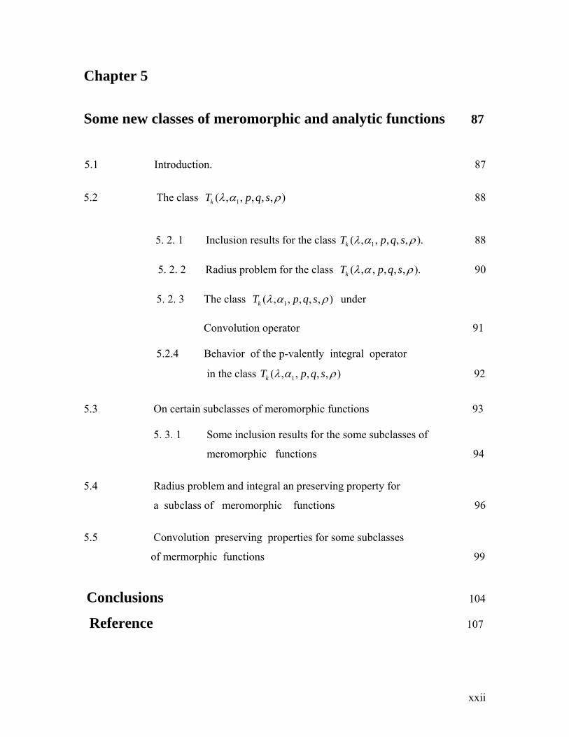
Chapter 5
Some new classes of meromorphic and analytic functions 87
5.1 Introduction. 87
5.2 The class 1( , , , , , )kT p q sλ α ρ 88
5. 2. 1 Inclusion results for the class 1( , , , , , ).kT p q sλ α ρ 88 5. 2. 2 Radius problem for the class ( , , , , , ).kT p q sλ α ρ 90 5. 2. 3 The class 1( , , , , , )kT p q sλ α ρ under
Convolution operator 91
5.2.4 Behavior of the p-valently integral operator
in the class 1( , , , , , )kT p q sλ α ρ 92
5.3 On certain subclasses of meromorphic functions 93
5. 3. 1 Some inclusion results for the some subclasses of
meromorphic functions 94
5.4 Radius problem and integral an preserving property for
a subclass of meromorphic functions 96
5.5 Convolution preserving properties for some subclasses
of mermorphic functions 99
Conclusions 104
Reference 107

xxiii
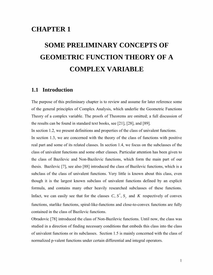
1
CHAPTER 1
SOME PRELIMINARY CONCEPTS OF
GEOMETRIC FUNCTION THEORY OF A
COMPLEX VARIABLE
1.1 Introduction
The purpose of this preliminary chapter is to review and assume for later reference some
of the general principles of Complex Analysis, which underlie the Geometric Functions
Theory of a complex variable. The proofs of Theorems are omitted; a full discussion of
the results can be found in standard text books, see [21], [28], and [89].
In section 1.2, we present definitions and properties of the class of univalent functions.
In section 1.3, we are concerned with the theory of the class of functions with positive
real part and some of its related classes. In section 1.4, we focus on the subclasses of the
class of univalent functions and some other classes. Particular attention has been given to
the class of Bazilevic and Non-Bazilevic functions, which form the main part of our
thesis. Bazilevic [7], see also [88] introduced the class of Bazilevic functions, which is a
subclass of the class of univalent functions. Very little is known about this class, even
though it is the largest known subclass of univalent functions defined by an explicit
formula, and contains many other heavily researched subclasses of these functions.
Infact, we can easily see that for the classes ,C *,S Sγ and K respectively of convex
functions, starlike functions, spiral-like-functions and close-to-convex functions are fully
contained in the class of Bazilevic functions.
Obradovic [78] introduced the class of Non-Bazilevic functions. Until now, the class was
studied in a direction of finding necessary conditions that embeds this class into the class
of univalent functions or its subclasses. Section 1.5 is mainly concerned with the class of
normalized p-valent functions under certain differential and integral operators.
2
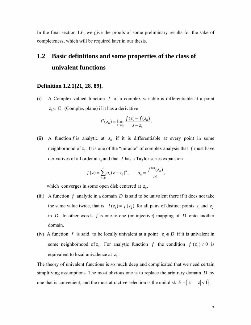
In the final section 1.6, we give the proofs of some preliminary results for the sake of
completeness, which will be required later in our thesis.
1.2 Basic definitions and some properties of the class of
univalent functions
Definition 1.2.1[21, 28, 89].
(i) A Complex-valued function f of a complex variable is differentiable at a point
0z ∈ (Complex plane) if it has a derivative
0
00
0
( ) ( )( ) lim .z z
f z f zf zz z→
−′ = −
(ii) A function f is analytic at 0z if it is differentiable at every point in some
neighborhood of 0z . It is one of the “miracle” of complex analysis that f must have
derivatives of all order at 0z and that f has a Taylor series expansion
00
( ) ( ) ,nn
nf z a z z
∞
=
= −∑ ( )
0( ) ,!
n
nf za
n=
which converges in some open disk centered at 0.z (iii) A function f analytic in a domain D is said to be univalent there if it does not take
the same value twice, that is 1 2( ) ( )f z f z≠ for all pairs of distinct points 1z and 2z
in D . In other words f is one-to-one (or injective) mapping of D onto another
domain.
(iv) A function f is said to be locally univalent at a point 0z D∈ if it is univalent in
some neighborhood of 0z . For analytic function f the condition 0( ) 0f z′ ≠ is
equivalent to local univalence at 0z .
The theory of univalent functions is so much deep and complicated that we need certain
simplifying assumptions. The most obvious one is to replace the arbitrary domain D by
one that is convenient, and the most attractive selection is the unit disk { }: 1E z z= < .
3
If ( )g z is analytic in E , it has a Maclaurin expansion
20 1 2
0( ) ... ,n
nn
g z b b z b z b z∞
=
= + + + = ∑
that is convergent in E . We note that if ( )g z is univalent in ,E then the addition of
constant merely translates the image domain so that ( )g z c+ is again univalent in E .
Consequently, in the above series the constant term 0b is arbitrary. As a first step toward
normalization we subtract 0b and consider 0( ) .g z b− We next observe that if 0( ) 0,g z′ =
then ( )g z is not univalent in any neighborhood of 0.z Consequently if ( )g z is univalent
in ,E then 1 (0) 0.b g′= ≠ Hence we may divide by 1b and consider 0
1
( )( ) .g z bf zb
−=
Since multiplication by 1
1b
merely rotates and stretches (or shrinks) the image domain,
we see that if ( )g z is univalent in D then 0
1
( )( ) g z bf zb
−= is also univalent in the same
domain and conversely, if ( )f z is univalent in ,D then so also is ( )g z . Setting 1
nn
b ab
= in
the above series, we have the following normalization form
2 32 3
2
( ) ... .nn
n
f z z a z a z z a z∞
=
= + + + = + ∑ (1.2.1)
(v) A function of the form (1.2.1) is said to be normalized univalent if ( )f z is univalent
and has the form (1.2.1), it is called a normalized univalent function. The class of
all normalized univalent functions in ,E is denoted by S and we also denote byA ,
the class of all analytic functions in .E
(vi) If ( )f z and ( )g z are analytic in E , we say that ( )f z is subordinate to ( )g z ,
written symbolically as follows:
≺f g in E or ( ) ( ), ,≺f z g z z E∈
if there exists a Schwarz function ( ),w z which by definition is analytic in E with
(0) 0w = and ( ) 1 ( )w z z E< ∈ ,
4
such that
( )f z = ( ( )),g w z ( ).z E∈
Indeed, it is known that
( ) ( ), (0) (0)≺f z g z z E f g∈ ⇒ = and ( ) ( ).f E g E⊂
Furthermore, if the function )(zg is univalent in ,E then we have the following
equivalence, see [44]; see also [59, p-4].
( ) ( ),≺f z g z z E∈ (0) (0)f g⇔ = and ( ) ( ).f E g E⊂
The concept of subordination between analytic functions can be traced back to
Lidelof [42], although Littlewood [43,44] and Rogosinski [95, 96] introduced the term
and established the basic results involving subordination. Quite recently, Srivastava and
Owa [107] investigated various interesting properties of the generalized hypergeometric
function by applying the concept of subordination.
The leading example of a function of class S is the Koebe function,
2 3
21
( ) 2 3 ... .(1 )
n
n
zk z z z z nzz
∞
=
= = + + + =− ∑ (1.2.2)
The Koebe function maps the disk ,E one-one and conformally onto the entire plane
minus the part of the negative real axis from 14
− to infinity ( −∞ ). This is best seen by
writing
21 1 1( )
4 1 4zk zz
+⎛ ⎞= −⎜ ⎟−⎝ ⎠
and observing that the function
0
1( )1
zL z wz
+= =
−
maps E conformally onto the right halp plane Re( ) 0.w > The class S is preserved under a number of elementary transformations
5
1.3 The class Ρ of functions with positive real part and some of its related classes
The class of functions with positive real part plays a crucial rule in the Geometric
Function Theory. Its significance can be seen from the fact that all the simple subclasses
of the class of univalent functions have been defined by using the concept of the class of
functions with positive real part. In this section, we define the class of functions with
positive real part and we presents here some of its interesting properties, such as its
relation with the class of univalent functions, for more details, see [28]. In addition, we
define some of its related classes.
1.3.1 The class Ρ [26, 21 ]
The class Ρ is the set of all functions of the form
21 2
1( ) 1 ... ... 1 ,n n
n nn
p z c z c z c z c z∞
=
= + + + + + = + ∑ (1.3.1)
that are analytic in ,E and such that for z in ,E Re ( ) 0.p z > Any function in Ρ is
called a function with positive real part in .E
It should be noted that ( )p z is not necessarily required to be univalent. Thus
( ) 1 np z z= + is in Ρ for any integer 0,n ≥ but if 2,n ≥ the function is not univalent.
Just as the Koebe function plays a central role in the class ,S the Möbius function
20
1
1( ) 1 2 2 ... 1 21
n
n
zL z z z zz
∞
=
+= = + + + = +
− ∑ , (1.3.2)
plays a central role in the class Ρ. The function defined by (1.3.2) is in the class Ρ, it is
analytic and univalent in ,E and it maps E onto the right half-plane .H + There is one
notable difference in the character of 0 ( )L z and ( )k z . In many extremal problems for
the class ,S the Koebe function is the unique solution (apart from a rotation). In contrast,
the function 0 ( )L z does maximize nc in the class Ρ, but if 2,n ≥ there are infinitely
6
many other functions in Ρ for which 2,nc = and no one of these is obtainable from any
other by a rotation, see [Theorem 3, 28]. The class Ρ is convex, see [28 ].
Theorem 1.3.1 [28] (The Herglotz Representation Theorem).
Let ( )tμ be a non-decreasing function in the interval 0 2 ,t π≤ ≤ with
2
0
( ) 2 ,d tπ
μ π=∫ (1.3.4)
then the function 2 2
00 0
1 1 1( ) ( ) ( ) ( ),2 1 2
itit
it
zef z d t L e d t z Eze
π π
μ μπ π
−−
−
+≡ ≡ ∈
−∫ ∫ (1.3.5)
is in Ρ. This theorem has been proved by Herglotz, [30] in 1911 and it is shown that the
converse of this theorem is also true that is, for each ( )f z in Ρ there is an associated
non-decreasing function ( )tμ for which (1.3.4) and (1.3.5) hold.
Theorem 1.3.2 [28] (Distortion Theorem for the class Ρ ).
If ( )p z is in Ρ, then for 1z r= <
1 1( ) ,1 1
r rp zr r
− +≤ ≤
+ −
and
2
2( ) .(1 )
p zr
′ ≤−
These inequalities are sharp. Equality occurs if and only if 0( ) ( ),ip z L e zα= where
0 ( )iL e zα is defined by (1.3.2).
In 1935, Noshiro [77] and Warschawski [119] independently proved a theorem, which is
called Noshiro-Warschawski Theorem and shows a beautiful relationship between the
class Ρ and .S
7
Theorem 1.3.3 [ 26] (The Noshiro-Warschawski Theorem).
Suppose that for some ,α Re( ( )) 0,ie f zα ′ ≥ for all z in a convex domain D. Then ( )f z is
univalent in D.
1. 3. 2 The Class Ρ(ρ) [28]
The class ( ),Ρ ρ is the subset of the class Ρ of functions p for which
Re ( ) , , 1.p z z Eρ ρ> ∈ 0 ≤ <
( )p Ρ ρ∈ can also be written as
2
0
1 1 (1 2 )( ) ( )2 1
it
it
zep z d tze
π ρ μ−
−
+ −=
−∫ , (1.3.6)
where ( )tμ is a function with bounded variation on [0, 2 ]π such that
2
0
( ) 2d tπ
μ =∫ and 2
0
( ) .d t kπ
μ ≤∫
We can write for ( )p Ρ ρ∈ as
1( ) (1 ) ( ) ,p z p zρ ρ= − + where 1 , .p z EΡ∈ ∈
1.3.3 The class Ρ[A,B] [28, 31]
In [31], Janowski introduced the class [ , ].A BΡ For A and B , 1 1,B A− ≤ < ≤ a
function ,p analytic in E with (0) 1p = belongs to the class [ , ]A BΡ if ( )p z is
subordinate to 1 .1
AzBz
++
In particular [ , ] [1, 1]A BΡ Ρ Ρ.⊂ − =
We also note that a function [ , ]p A BΡ∈ if and only if
8
2 2
1( ) , ( 1, )1 1
AB A Bp z B z EB B
− −− < ≠ ± ∈
− −
In addition, it is known [71] that [ , ]A BΡ is a convex set. Furthermore, it can easily be
shown that [ , ]p A BΡ∈ if, and only if there exists a function h Ρ∈ such that
(1 ) (1 ) ( )( ) .(1 ) (1 ) ( )
A A h zp zB B h z
− + +=
− + +
Next, for real parameters A and B such that 1 1,B A− ≤ < ≤ we define the function
1( , ; ) , ( ; 1 1).1
Azh A B z z E B ABz
+= ∈ − ≤ < ≤
+
Then it is known that the function ( , ; )h A B z is the conformal map of E onto a disk,
symmetrical with respect to the real axis, which is centered at the point
( )2
1 1 ,1
AB BB
−≠ −
−
and with radius equal to
21A B
B−
− and 1.B ≠ −
Furthermore, the boundary circle of this disk intersect the real axis at the points
1 1and ( 1, 1).1 1
A A BB B
− +≠ −
− +
Special selections of A and B lead to a familiar sets defined by inequalities, see [28].
Some of these are given below. Under the condition (0) 1,p = and 0 1,ρ≤ <
(i) [1, 1]Ρ − is the class Ρ of functions p with positive real part, that is Re ( ) 0p z >
in E.
(ii) [1 2 , 1]Ρ ρ− − is the class ( )Ρ ρ of functions p with Re ( )p z ρ> in E.
(iii) [1,0]Ρ is the class of function p defined by ( ) 1 1.p z − <
9
1.3.3 The class kΡ (ρ)[82]
Let ( )kΡ ρ be the class of functions ( )p z analytic in E satisfying the properties (0) 1p = and satisfying the condition
2
0
Re ( ) ,1p z d k
π ρ θ πρ
−≤
−∫ (1.3.7)
where , 2iz re kθ= ≥ and 0 1.ρ≤ < This class has been introduced in [91]. We note
that for 0,ρ = we obtain the class kΡ , see [87] and for 0,ρ = 2,k = we have the
well-known class Ρ of functions with positive real part. The case 2k = gives the
class ( )Ρ ρ of functions with positive real part greater than .ρ
Also we can write (1.3.7) as
2
0
1 1 (1 2 )( ) ( ),2 1
it
it
zep z d tze
π ρ μ−
−
+ −=
−∫
where ( )tμ is a function with bounded variation on [0,2 ]π such that, for 2,k ≥
2
0
( ) 2 ,d tπ
μ π=∫ and 2
0
( )d t kπ
μ ≤∫
From (1.3.7) we can easily deduce that that ( )kp Ρ ρ∈ if, and only if, there exist
1 2, ( ),p p Ρ ρ∈ such that for ,z E∈
1 21 1( ) ( ) ( ).
4 2 4 2k kp z p z p z⎛ ⎞ ⎛ ⎞= + − −⎜ ⎟ ⎜ ⎟
⎝ ⎠ ⎝ ⎠ (1.3.8)
It is known, see [67] that ( )kΡ ρ is a convex set.
10
1.4 Some classes of analytic functions
In this section, we are primarily concerned with some well-known classes of analytic
functions.
1.4.1 The class of starlike and convex Functions [21, 28]
A set D ⊂ is said to be starlike with respect to a point 0w D∈ if and only if the linear
segment joining 0w to every other point w D∈ lies entirely in .D The set D is said to
be convex if and only if it is starlike with respect to each of its points, that is if and only if
the linear segment joining any two points of D lies entirely in D . Let f ∈A and let f
be univalent in E . Then f maps E onto a convex domain, if and only if
( )Re 1 0( )
zf zf z
′′⎧ ⎫+ >⎨ ⎬′⎩ ⎭
, .z E∈ (1.4.1)
Such function f is said to be convex in E (or briefly convex). The condition of (1.4.1)
was first stated by Study [101]. Löwener [52] also studied the class of convex functions.
The set of all convex function is denoted by .C
Now let ,f ∈A (0) 0f = and let f be univalent in E . Then f maps E onto a starlike
domain with respect to 0 0w = if and only if
( )Re 0( )
zf zf z
′⎧ ⎫>⎨ ⎬
⎩ ⎭ , .z E∈ (1.4.2)
Such function f is said to be starlike in E with respect to 0 0w = (or briefly starlike).
We denote the set of all starlike functions by .S ∗ The class S ∗ was first studied by
Alexander [2]. The Condition (1.4.2) for starlikeness is due to Nevanlinna [63]. It is well-
known that if any analytic function f satisfies (1.4.2) and (0) 0, (0) 0,f f ′= ≠ then f is
univalent and starlike in E. One can alter the condition (1.4.1) and (1.4.2) by setting other
11
limitations on the behavior of ( )( )
zf zf z
′ and of ( )
( )zf zf z
′′′
in .E In this way many interesting
classes of analytic functions have been defined, see [26].
In 1936, Robertson introduced in [94] the classes *( ),S ρ ( )C ρ of starlike and
convex functions of order ρ , 0 1,ρ≤ < which are defined by
( )( ) : Re , 0 1,( )
zf zS f z Ef z
ρ ρ ρ∗ ⎡ ⎤′⎧ ⎫= ∈ > ≤ < ∈⎨ ⎬⎢ ⎥
⎩ ⎭⎣ ⎦A
( )( ) : Re 1 , 0 1,( )
zf zC f z Ef z
ρ ρ ρ⎡ ⎤′′⎧ ⎫
= ∈ + > ≤ < ∈⎨ ⎬⎢ ⎥′⎩ ⎭⎣ ⎦A
In particular * *(0) , (0) ,S S C C= =
where *S is the class of starlike functions with respect to origin and C is the class of
convex functions.
Thus * .C S S⊂ ⊂ Note that the Koebe function defined by (1.1.2) is starlike but not
convex. There is a closely analytic connection between convex and starlike mapping.
Alexander [2] first observed this in 1915. Strohhacker, see [110], gives another important
relation.
f C∈ in E , then 1 2( )f S∗∈ .
Theorem 1.4.1 [28] (Alexander Theorem).
Let f be analytic in E with (0) 0f = and (0) 1.f ′ = Then f C∈ if and only if
*( ) .zf z S′ ∈
Various inequalities for the class ,S such as the growth and distortion theorems, remains
sharp in *S because the Kobe function is starlike and is extremal in the full class .S
However, these estimates can be improved for the class C , which excludes the Koebe
function.
12
1.4. 2 The class of alpha –convex functions [28,60]
In 1969, P. Mocannu [60] introduced the concept of an alpha-convex or alpha-starlike
functions.
A function f given by (1.2.1) is said to be α − convex in the open unit disk ,E if it is
analytic, ( ) ( ) 0f z f zz
′≠ and
( ) ( ( ))(1 ) 0,( ) ( )
zf z zf zRef z f z
α α′ ′ ′⎧ ⎫
− + >⎨ ⎬′⎩ ⎭ for .z E∈
The set of all such function is denoted by .Mα
We note that the definition is meaningful if we consider α a complex number, but here
we will assume that α is real. If 1,α = then an α − convex function is convex; and if
0,α = then an α − convex function is starlike. In 1973 [57 ], it was proved that all
α- convex functions are convex if α ≥ 1 and starlike if α <1.
The class ( )kM α of functions with bounded Mocanu variation was introduced in
[20].
Let f be of the form (1.2.1) analytic and locally univalent in E . Then for
2, 0, ( )kk f Mα α≥ ≥ ∈ if and only if
( ) ( ( ))(1 ) .( ) ( ) k
zf z z f zf z f z
α α Ρ′ ′ ′⎡ ⎤
− + ∈⎢ ⎥′⎣ ⎦
1.4.3 The class K of close-to-convex functions [21, 28]
We now turn to an interesting subclass of S which contains *S and has a simple
geometric description. This is the class of close-to-convex functions introduced by
Kaplan [35] in 1952.
A function ,f ∈A is said to be close-to-convex, if and only if
13
( )Re 0,( )
zf z z Eg z
′> ∈ (1.4.3)
for some *.g S∈ Or equivalently if
( )Re 0, ,( )
f z z EG z
′> ∈
′
for some .G C∈ We shall denote by K the class of close-to-convex functions. A
necessary and sufficient condition that ,f of the form (1.2.1) normalized by the
conditions (0) 0, (0) 1f f ′= = and ( ) 0f z′ ≠ in E is close-to-convex is that, for every
r in (0,1) and every pair 1 2,θ θ with 1 20 2 ,θ θ π≤ ≤ ≤ we have
2
1
( ( ))Re ,( )
z f z df z
θ
θ
θ π′ ′⎧ ⎫
> −⎨ ⎬′⎩ ⎭∫ (1.4.4)
where .iz re θ= From (1.4.4), it is clear that f K∈ implies that f maps each circle
1z r= < onto a simple closed curve whose tangent rotates, as θ increases, either in the
counterclockwise direction or clockwise direction in such a way that it never turns back
on itself so much as to completely reverse its direction.
The class K has been introduced independently and in a quite different manner by
Biernacki [10], see [9]. The close-to-convex functions are univalent, see [35] and the
class K proved the most useful subclass of S .
We note that convex and starshaped domains are close-to-convex. The class K is of
considerable importance in as much as it contains most of the known subclasses of S,
this can be summarized as:
.C S K S∗⊂ ⊂ ⊂ Goodman in [29] defines the class ( )K ρ of function as follows.
Let f given by (1.2.1) be analytic in ,E with ( ) 0.f z′ ≠ Then for 0, ( ),f Kρ ρ> ∈ if
for iz re θ= and 1 2θ θ<
2
1
( ( ))Re .( )
z f z df z
θ
θ
θ ρπ′ ′⎧ ⎫
> −⎨ ⎬′⎩ ⎭∫
14
1.4.4 The class kV of functions with bounded boundary
rotation [21, 28]
In [52], Löwner introduced the concept of bounded boundary rotation and using this
Paatero [84], showed that if ,f ∈A is locally univalent and maps E onto a domain of
bounded boundary rotation, then ( )f z′ has the following integral representation.
2
0
1( ) exp log(1 ) ( ) ,if z ze dπ
θ μ θπ
−⎧ ⎫−⎪ ⎪′ = −⎨ ⎬⎪ ⎪⎩ ⎭
∫
where ( )μ θ is finite normalized measure satisfy
2
0
( )dπ
μ θ < ∞∫ , 2
0
( ) 2 .dπ
μ θ π=∫
A locally univalent function ,f ∈A is in the class ,kV if it map the unit disc E
conformlly onto a domain whose boundary rotation is at most πk . Since the boundary
rotation is the total variation of the argument of the boundary tangent vector (whenever
such a tangent vector exists), we have 2
0
( )Re 1 ,( )
i i
i
re f re d kf re
π θ θ
θ θ π′′⎛ ⎞
+ ≤⎜ ⎟′⎝ ⎠∫ (1.4.5)
for all (0,1),r ∈ θirez = and 2k ≥ . It is well known [11] that for kf V∈ , there exists two starlike functions 1S and 2S such that
14 2
1
14 2
2
( )
( ) .( )
k
k
S zzf z
S zz
−
+
⎛ ⎞⎜ ⎟⎝ ⎠′ =⎛ ⎞⎜ ⎟⎝ ⎠
Clearly, if 1 2 ,k k< then 1 2
.k kV V⊂
We observe that without absolute value sign (1.4.5) yields
2
0
( )Re 1 2 ,( )
i i
i
re f re df re
π θ θ
θ θ π′′⎛ ⎞
+ =⎜ ⎟′⎝ ⎠∫
15
so that we must have 2k ≥ in (1.4.5). Further if 4,k ≤ then ( )f z is close-to-convex by
(1.4.4). However, the converse is not true. If ( )f z maps E onto the domain formed by
deleting an infinite number of vertical slits from the plane, then ( )f z is close-to-convex,
but ( )f z is not in kV for any .k
The classes kV obviously expand as k increases. 2V is simply the class C of convex
mappings. Pattero[ 84] showed that 4 .V S⊂
It is interesting to consider extremal problems within the class kV . The Koebe functions
belongs to 4V but not to kV for any 4,k < so even the standard growth and distortion
problems will have new solutions for 4.k < For arbitrary 2,k ≥ Lowner [52] obtained
the sharp distortion theorem
1 12 2
1 12 2
(1 ) (1 )( ) , 1,(1 ) (1 )
k k
k kr rf z z rr r
− −
+ +
− +′≤ ≤ = <+ −
for all ,kf V∈ with equality only for certain rotations of the “wedge mapping”
2
2
1 1 1( ) ( ) 1.1
K
nk n
N
zF z z B k zk z k
ςς ς
∞
=
+⎛ ⎞= − = + =⎜ ⎟−⎝ ⎠∑ (1.4.6)
This function plays the role of the Koebe function in kV . In particular, 4F is the Koebe
function and 2F is the half-plane mapping 1( ) (1 ) ,l z z z −= − the typical extremal function
for problems involving convex functions.
The radius R of convexity of circle, which kf V∈ maps into a convex domain is at least
21 4 ,2
R k k⎡ ⎤= − −⎣ ⎦
(1.4.7)
and this is best possible as can be seen from the function k kF V∈ defined by (1.4.6). This
result has been first found by Paatero in [83].
In [12], the author proved that kV is contained in the class ( )K ρ of close-to-convex
functions of order ρ , where 1.2kρ = − Part of the result was proved first by Brannan [11]
16
and that was for 2 4.k≤ ≤ For 1ρ > the class ( )K ρ properly contains the class
(1)K K= of close-to-convex functions.
1.4.5 The class kR of functions with bounded radius rotation [65, 66 ]
The class kR was first introduced by Tammi [ 112] and later it was discussed in
[92, 65, 66].
Let f ∈ ⋅A Then f is said to be in the class kR of functions with bounded radius
rotation if, for (0 1),iz re rθ= < < ( ) 0f zz
≠ ,
2
0
( )Re , 2.( )
zf z d k kf z
π
θ π′
≤ ≥∫
It is clear that kf V∈ , if and only if, .kzf R′∈ From this relation we see that k kV R⊂ .
We note that *2 ,R S= the class of starlike functions with respect to origin.
Also we define that ,kf R∈ if and only if ( ) .( ) k
zf zf z
Ρ′
∈
1.4.6 The class kR (ρ) [65, 66]
Let f ∈ ⋅A Then f is said to be in the class E . Then for 2, 0 1, ( )kk f Rρ ρ≥ ≤ < ∈ if it satisfies the condition:
2
0
( )( )Re1
zf zf z d k
π ρθ π
ρ
′−
≤−∫ .
Also a function ,f analytic in E and given by (1.2.1) is said to belong to the class
( ), 2, 0 1,kR kρ ρ≥ ≤ < if and only if
( ) ( ).( ) k
zf zf z
Ρ ρ′
∈
Clearly *2 ( ) ( )R Sρ ρ= and (0) ,k kR R= the class of functions of bounded radius
rotations, see [37].
17
1.4.7 The class kV (ρ) [82]
The class ( )kV ρ of functions with bounded boundary rotation of order ρ was first introduced in [82]. A function f analytic in E and given by (1.2.1) belongs to ( )kV ρ for z E∈ if and only if
( ( )) ( ), 0 1, 2.( ) k
zf z kf z
Ρ ρ ρ′ ′
∈ ≤ < ≥′
It is obvious that
( ),kf V ρ∈ if and only if, ( ) ( ).kzf z R ρ′ ∈
It may be noted that 2 ( ) ( ),V Cρ ρ= the class of convex functions of order ,ρ see [94]
and (0) ,k kV V= the class of functions of bounded Boundary rotations first discussed by
Paatero, see [84]. It can easily be seen, see [82] that ( )kf V ρ∈ if and only if there
exists kF V∈ such that 1( ) ( ( )) .f z F z ρ−′ ′= 1.4.8 The class of Bazilevic functions [56, 114]
If ( )g z is starlike (with respect to the origin) in ,E ( )p z is analytic with Re ( ) 0p z > in
,E α is any real number and 0,β > then
1
1
0
( ) ( ) ( ) ( )z i
if z i p g dβ α
β αβ α ζ ζ ζ ζ+
−⎡ ⎤= +⎢ ⎥
⎣ ⎦∫ (1.4.8)
has been shown by Bazilevic [7], see also [88], to be analytic and univalent function in E .
The powers appearing in the formula are meant as principal values. We shall denote by
( , , , )B p gα β the class of functions defined by (1.4.8).
If we put 0α = in (1.4.8) then we have
1
0
1
,( ) ( ) ( )z
f z p g dβ ββ ζ ζ ζ ζ−⎡ ⎤
= ⎢ ⎥⎣ ⎦
∫
18
and on differentiating this expression we obtain 1( ) ( ) ( ) ( ),zf z f z g z p zβ β−′ = (1.4.9)
We shall call a function satisfying (1.4.9) a Bazilevic function of type .β
Very little is known about ( , , , )B p gα β in general, even though it is the largest known
subclass of univalent functions defined by and explicit formula, and contains many of the
heavily researched classes of univalent functions. Infact, we can easily see that for the
classes of convex function ,C starlike functions *,S spiral-like-functions Sγ and close-
to-convex functions ,K we have
(i) (0,1,1, ).C B g=
(ii) (0,1, , )zgS B gg
∗ ′=
(ii) ( , , , ).zgS B sin cos cos gg isinγ γ γ
γ′
=+
(iv) (0,1, , )K B p g=
The Bieberbach conjecture remains unsettled for Bazilevic functions. J. Zamorski [123]
has shown the conjecture valid for the class 1(0, , , )B p gN
where N is a positive integer.
D. K. Thomas [114] has shown that if 0
( ) nn
nf z a z
∞
=
= ∑ is in (0, , , )B p gβ and is bounded,
then 1 .na On
⎛ ⎞= ⎜ ⎟⎝ ⎠
1.4.9 The class of Non-Bazilevic functions [78,118]
Assume that 0 1.α< < Then a function f ∈A is in the class of non-Bazilevic functions
denoted by ( )N α if and only if
1
Re ( ) 0, .( )zf z z E
f z
α+⎧ ⎫⎛ ⎞⎪ ⎪′ > ∈⎨ ⎬⎜ ⎟⎝ ⎠⎪ ⎪⎩ ⎭
(1.4.10)
19
( )N α was introduced by Obradovic [78]. He called this class of functions to be of non-
Bazilevic type. Until now, the class was studied only in a direction of finding necessary
conditions over α that embeds this class into the class of univalent functions or its
subclass.
1.5 P-valent functions and certain differential and integral
operators
This section is mainly concerned with the class of normalized p-valent functions. We also
give the definitions of certain known differential and integral operators, which will be
required in our later sections.
1.5.1 Hypergeometric function and Hadmard
product (or convolution) [86]
Let ,f g ∈A be given by
2 2( ) and ( ) .n n
n nn n
f z z a z g z z b z∞ ∞
= =
= + = +∑ ∑
We define the convolution operator : by ( )g f gΦ → Φ = ∗A A for a given
,f ∈A where
2
( )( ) ,nn n
nf g z z a b z
∞
=
∗ = + ∑
denote the Hadmard product (or convolution) of the function ( )f z and ( ).g z
Let ( )pA denote the class of functions ( )f z normalized by
1
( ) , ( {1,2,3...,})p p kp k
k
f z z a z p∞
++
=
= + ∈ =∑ (1.5.1)
which are analytic and p-valent in the unit disk .E
For functions ( ) ( ),jf z p∈A and given by
20
,1
( ) ( 1, 2),p p kj p k j
kf z z a z j
∞+
+=
= + =∑
we define the Hadamard product (or convolution) of 1 2( ) and ( )f z f z by
1 2 ,1 ,2 2 11
( )( ) ( )( ).p p kp k p k
kf f z z a a z f f z
∞+
+ +=
∗ = + = ∗∑ (1.5.2)
In our present investigation, we shall make use of the Gauss hypergeometric function
defined by
2 10
( ) ( )( , ; ; ) ( , ; ; ) ,( ) (1)
kk k
k k k
a bF a b c z G a b c z zc
∞
=
= = ∑ (1.5.3)
where , ,a b c ∈ , { }0 0, 1, 2, 3,...c −∉ = − − − and )k(ν denote the Pochhammer symbol
(or the shifted factorial) given, in terms of the Gamma function Γ , by
{ }1 if 0 and \ 0 ,( )( ) ( 1)...( 1) if and
( )k
k vv kv v v v k k v
v
⎧ = ∈⎪Γ +
= = + + − ∈ ∈⎨Γ ⎪⎩
We note that the above series defined by (1.5.3) converges absolutely for z E∈ and
hence ( , ; ; )G a b c z represents an analytic function in the open unit disk E, see
[120, chapter 14]. For the properties of hypergeometric function, see Lemma 1.6.10.
1. 5. 2 Ruscheweyh Derivatives [27,68]
Denote by 1 : ( ) ( )n pD p p+ − →A A the operator defined by
1 ( ) ( ), ( ( ) ( ))(1 )
pn p
n p
zD f z f z f z pz
+ −+= ∗ ∈
−A (1.5.4)
1` 1( ( )) ,
( 1)!
p n n pz z f zn p
− + −
=+ −
21
where n is any integer greater than .p− The symbol 1n pD + − when 1p = was introduced
by Ruscheweyh [98], and the symbol 1n pD + − was introduced by Goel and Sohi [27].
Therefore, we call the symbol 1n pD + − to be the Ruscheweyh derivative of ( 1)n p th+ −
order. It follows from (1.5.4) that
1 1( ( )) ( ) ( ) ( ).n p n p n pz D f z n p D f z nD f z+ − + + −′ = + −
1. 5. 3 The generalized Livingston-Libra-Bernardi operator [86]
For a function ( ) ( )f z p∈A and ,pδ > − the integral operator , : ( ) ( )p p pδ →A AF
is defined by , see [19].
1,
0
( )( ) ( )z
p p
pf z t f t dtz
δδ
δ −+= ∫F
1
( ).p p k
k
pz z f zp k
δδ
∞+
=
⎛ ⎞+= + ∗⎜ ⎟+ +⎝ ⎠
∑ (1.5.5)
It easily follows from (1.5.5) that
( ( , ) ( ) ( )) ( ) ( , ) ( ) ( , ) ( )( ).p p pz I a c f z p I a c f z I a c f zλ λ λ
δ δδ δ′ = + −,p ,pF F (1.5.6)
1. 5. 4 The operator ( , )p a cL [86]
We now define a function ( , ; )p a c zφ by
1
( )( , ; ) ,( )
p p kkp
k k
aa c z z zc
φ∞
+
=
= + ∑ (1.5.7)
( )0, \ {0, 1, 2, 3,...} .a c −∈ ∈ = − − −
Corresponding to the function ( , ; )p a c zφ given by (1.5.7), we consider a linear operator
( , )a cpL , which is defined by means of the following Hadamard product (or
convolution).
22
( , ) ( ) ( , ; ) ( ), ( ( ) ( )).p pa c f z a c z f z f z pφ= ∗ ∈L A (1.5.8)
It is easily seen from (1.5.8) that
( )( , ) ( ) ( 1, ) ( ) ( )( ( , ) ( )).p p pz a c f z a a c f z a p a c f z′ = + − −L L L
We also note that
( , ) ( ) ( )p a a f z f z=L , ( )( 1, ) ( )p
zf zp p f zp′
+ =L ,
and
1( ,1) ( ) ( ), ( ),n pP n p f z D f z n p+ −+ = > −L
where in the special case when 1p = and 0 0( {0}),∪n∈ = nD can be identified
with the Ruscheweyh derivative of order ,n see for details [98].
The linear operator ( , )a cpL defined by (1.5.8), was introduced and studied by Saitoh
[99] on the space of analytic and p-valent functions in .E It was motivated essentially by
the familiar Carlson-Shaffer operator [13] given by (1.5.8) for 1.p = The Carlson-
Shaffer operator includes, as its further special cases, not only the above mentioned
Ruscheweyh derivative, but also some families of fractional calculus operators which are
investigated rather extensively in the theory of analytic and univalent functions, see
[105, 106].
1.5.5 The Noor integral operator n+ p-1I [68]
Let 1 ( ) , ( )(1 )
p
n p n p
zf f z n pz+ − += > −
− and let ( 1)
1( )n pf z−+ − be defined such that
( 1)1 1( ) ( )
(1 )
p
n p n p p
zf z f zz
−+ − + −∗ =
− . (1.5.9)
Analogous to symbol 1,n pD + − we here define an integral operator
1 : ( ) ( )n pI p p+ − →A A as follows.
23
( 1)1 1( ) ( )( )n p n pI f z f f z−
+ − + −= ∗
( 1)
( ), ( ).(1 )
p
n p
z f z n pz
−
+
⎡ ⎤= ∗ > −⎢ ⎥−⎣ ⎦
(1.5.10)
With 0I f zf ′= and 1 ,I f f= we refer to Noor [ 51, 69, 70, 73, 74] and [14] for more
details. From (1.5.9) and (1.5.10), we obtain the following identity for the operator n pI +
1( ( )) ( ) ( ) ( ).n p n p n pz I f z n p I f z nI f z+ + − +′ = + −
1.5.6 The Cho − Kown − Srivastava integral operator λ
pI (a,c)[86]
With the aid of the function ( , ; )p a c zφ defined by (1.5.7), we consider a function
(†) ( , ; )p a c zφ defined by
(†)( , ; ) ( , ; ) , ,(1 )
p
p p p
za c z a c z z Ez λφ φ +∗ = ∈
− (1.5.11)
where .pλ > − This function yields the following family of linear operators (†)( , ; ) ( ) ( , ; ) ( ), ,p pI a c z f z a c z f z z Eλ φ= ∗ ∈ (1.5.12)
where 0, \ {0, 1, 2, 3,...}a c −∈ = − − − . For a function ( ),f p∈A given by (1.5.1), it
follows from (1.5.12) that for pλ > − and 0, \a c −∈
1
( ) ( )( , ) ( )( ) (1)
p p kk kp p k
k k k
c pI a c f z z a za
λ λ∞+
+=
+= + ∑ (1.5.13)
( , , ; ) ( ), .pz G c p a z f z z Eλ= + ∗ ∈
From equation (1.5.13), we deduce that
1( ( , ) ( )) ( ) ( , ) ( ) ( , ) ( ),p p pz I a c f z p I a c f z I a c f zλ λ λλ λ+′ = + − (1.5.14)
and
( ( 1, ) ( )) ( , ) ( ) ( ) ( 1, ) ( ).p p pz I a c f z a I a c f z a p I a c f zλ λ λ′+ = − − + (1.5.15)
24
We also note that
0
0
( )( 1,1) ( ) ,z
pf tI p f z p dtt
+ = ∫
0 1( ,1) ( ) ( 1,1) ( ) ( ),p pI p f z I p f z f z= + =
1 ( )( ,1) ( ) ,pzf zI p f z
p′
=
2
2 2 ( ) ( )( ,1) ( ) ,( 1)p
zf z z f zI p f zp p
′ ′′+=
+
2 ( ) ( )( 1,1) ( ) ,1p
f z zf zI p f zp
′++ =
+
and
1( , ) ( ) ( ), , ,n n ppI a a f z D f z n n p+ −= ∈ > −
where 1n pD + − is the Ruscheweyh derivative of (n+p-1)th order, see [27].
The operator 0( , ) ( , , \ )pI a c p a cλ λ −> − ∈ was recently introduced by Cho et al
[16], who investigated (among other things) some inclusion relationships and argument
properties of various subclasses of multivalent functions in ( )A p , which were defined by
means of the operator ( , ).pI a cλ
For 1cλ = = and ,a n p= + the Cho − Kown − Srivastava operator ( , )pI a cλ yields
11( ,1) , ( ),p n pI n p I n p+ −+ = > −
where 1n pI + − denotes an integral operator of the (n+p-1)th order, which was studied by
Liu and Noor [51], see also [68,71]. The linear operator 1 ( 2,1), ( 1, 2)I λ μ λ μ+ > − > −
was also recently introduced and studied by Choi et al [17]. For relevant details about
further special cases of the Choi–Saigo − Srivastava operator 1̀ ( 2,1),I λ μ + the interested
reader may refer to the works by Cho et al [17] and Choi et al [16], see also [18, p-507].
25
1. 5. 7 The Dziok − Srivastava operator p,q,s 1H (α ) [50]
Making use of the Hadamard product (or convolution) given by (1.5.2), we now define
the Dziok − Srivastava operator,
1 1( ,..., ; ,... ) ; ( ) ( ),p q qH p pα α β β →A A
which was introduced and studied recently in a series of papers by Dziok and Srivastava
[22, 23], see also [46, 48].
For complex parameters
1 1 0,..., and ,..., , ( \ : {0, 1, 2,...}; 1,..., ),q s j j sα α β β β −∈ = − − =
we now define the generalized hypergeometric function 1 1( ,..., ; ,..., ; )q s q qF zα α β β
[80, 108] as follows:
11 1
0 1
( ) ...( )( ,..., ; ,..., ; ) : ,
( ) ...( ) !
kk q k
q s q sk k s k
zF z
kα α
α α β ββ β
∞
=
=∑ (1.5.16)
We note that the series ( )q sF z series in (1.5.16) converges absolutely for
| |z < ∞ if 1,q s< + and for z E∈ if 1.q s= +
Corresponding to a function 1 1( ,..., ; ,..., ; )p q s zα α β βF defined by
1 1 1 1( ,..., ; ,..., ; ) ( ,..., ; ,..., ; ).p
p q s q s q sz z F zα α β β α α β β=F
Dziok and Srivastava [22] considered a linear operator defined by the following
Hadamard product (or convolution):
1 1 1 1( ,..., ; ,..., ) ( ) ( ,..., ; ,..., ; ) ( ).p q s p q sH f z z f zα α β β α α β β= ∗F (1.5.17)
For convenience, we write
, , 1 1 1( ) : ( ,..., ; ,..., ).p q s p q sH Hα α α β β= (1.5.18)
{ } { }0( 1; , : 0 ; : 1, 2,... ; ),q s q s z E≤ + ∈ = ∪ = ∈
26
Thus, after some calculations, we have the following identity
, , 1 1 , , 1 1 , , 1( ( ) ( )) ( 1) ( ) ( ) ( ) ( ).p q s q s p q sz H f z H f z p H f zλα α α α α′ = + − − (1.5.19)
Many interesting subclasses of analytic functions, associated with the Dziok − Srivastava
operator , , 1( )p q sH α and its many special cases, have been investigated recently by Dziok
and Srivastava [22,23], Gangadharan et al [26], Liu [46], Liu and Srivastava [48], see
also [46,80,106].
1. 5. 8 Meromorphic analogue of the Choi-Saigo-Srivastava
operator λ,q,s 1H (α ) [15]
Let M denote the class of functions of the form
0
1( ) ,kk
kf z a z
z
∞
=
= + ∑
which are analytic in the punctured unit disk { } { }: and 0 1 \ 0 .E z z z E∗ = ∈ < < = .
Corresponding to a function 1 1( ,..., ; ,..., ; )q s zα α β βF defined by
11 1 1 1( ,..., ; ,..., ; ) ( ,..., ; ,..., ; ).q s q s q sz z F zα α β β α α β β−=� (1.5.20)
Liu and Srivastava [48] considered a linear operator
1 1( ,..., ; ,..., )q sH α α β β : M M→ defined by the following Hadamard product (or
convolution):
1 1 1 1( ,..., ; ,..., ) ( ) ( ,..., ; ,..., ; ) ( ).q s q sH f z z f zα α β β α α β β= ∗F (1.5.21)
We note that the linear operator 1 1( ,..., ; ,..., )q sH α α β β was motivated essentially by
Dziok and Srivastava [22]. Some interesting developments with the generalized
hypergeometric functions were considered recently in [23, 24,49,50] .
27
Corresponding to the function 1 1( ,..., ; ,..., ; )q s zα α β βF defined by (1.33.1), we
introduce a function 1 1( ,..., ; ,..., ; )q s zλ α α β βF given by
1 1 1 11( ,..., ; ,..., ; ) ( ,..., ; ,..., ; ) ( 0).
(1 )q s q sz zz zλ λα α β β α α β β λ∗ = >
−F F (1.5.22)
Analogous to 1 1( ,..., ; ,..., )q sH α α β β defined by (1.33.2), we now define the linear
operator 1 1( ,..., ; ,..., )q sHλ α α β β on M as follows:
1 1 1 1( ,..., ; ,..., ) ( ) ( ,..., ; ,..., ; ) ( )q s q sH f z z f zλ λα α β β α α β β= ∗F (1.5.23)
0( , \ ; 1,.., ; 1,..., ; 0; ; ).i j i q j s z E f Mα β λ− ∗∈ = = > ∈ ∈
For convenience, we write
, , 1 1 1( ) : ( ,..., ; ,..., ).q s q sH Hλ λα α α β β=
It is easily verified from the definition (1.33.3) and (1.33.4) that
, , 1 1 , , 1 1 , , 1( ( 1) ( )) ( ) ( ) ( 1) ( 1) ( ),q s q s q sz H f z H f z H f zλ λ λα α α α α′+ = − + + (1.5.24)
and
, , 1 1, , 1 , , 1( ( ) ( )) ( ) ( ) ( 1) ( ) ( ).q s q s q sz H f z H f z H f zλ λ λα λ α λ α+′ = − + (1.5.25)
We note that the operator , , 1( )q sHλ α is closely related to the Choi −Saigo −Srivastava
operator [17] for analytic functions, which includes the integral operator studied by Liu
[47] and Noor et al [70,74].
1.6 Preliminary results
This section contains several fundamental lemmas, which are essential for the proof of
the principal results. We give the proofs of some known lemmas which will be required
in our later discussions for the sake of completeness,
28
Definition 1.6.1 [59].
Let ( )E=H H denote the class of analytic functions in .E For n a positive integer and
,a ∈ let
[ ] { }11, : ( ) ... ,n n
n na n f f z a a z a z ++= ∈ = + + +H H (1.6.1)
with [ ]0 0,1 .≡H H
Let 3: Eψ × → and let h be univalent in .E If p is analytic in E and satisfies the
second order differential subordination
2( ( ), ( ), ( ); ) ( ),p z zp z z p z z h zψ ′ ′′ ≺ (1.6.2)
then p is called the solution of the differential subordination. The univalent function q
is called a dominant of the solutions of the differential subordination, or more simply a
dominant, if p q≺ for all p satisfying (1.6.2). A dominant q that satisfy q q≺ for
all dominant q of (1.6.1) is said to be the best dominant of (1.6.2). Note that the best
dominant is unique up to a rotation of .E
If we require the more restrictive condition [ ], ,p a n∈H then p will be called an
( , ) dominant,a n − and q the best ( , ) dominant.a n −
Defintion 1. 6. 2 [59].
Let Q denote the set of functions q that are analytic and injective on \ ( ),E U q where
{ }( ) : lim ( ) ,z
U q E q zς→∞
= ∈∂ = ∞ and are such that ( ) 0q ς′ ≠ for \ ( ).E U qς ∈∂
If q Q∈ then ( )q EΔ = is a simply connected domain and its boundary consists of
either a simple closed regular curve or the possibly infinite union of pair wise disjoint
simple regular curves, each of which converges to ∞ in both directions. The function
1( )q z z= and 21( )1
zq zz
+=
− are examples of these two cases.
Definition 1. 6. 3 [57, 58].
29
Let Ω be a set in , q Q∈ and n be a positive integer. The class of admissible
functions [ , ],n qΨ Ω consists of those functions 3: Eψ × → that satisfy the
admissibility condition:
( , , ; ) ,r s t zψ ∉Ω (1.6.3)
where ( ), ( ),r q s m qς ς ς′= =
We write 1[ , ] [ , ].q qΨ Ω ≡ Ψ Ω
In the special case when Ω is simply connected domain, ,Ω ≠ and h is a conformal
mapping of E onto Ω we denote this by [ , ].n h qΨ
If 3: Eψ × → , then the admissibility condition (1.6.3) reduces to
( ( ), ( ); ) ,q m q zψ ς ς ς′ ∉Ω
when , \ ( ) and .z E E U q m nς∈ ∈∂ ≥
If : Eψ × → , then the admissibility condition (1.6.3) reduces to
( ( ) ; ) ,q zςΨ ∉Ω when , \ ( ).z E E U qς∈ ∈∂
In addition, it is known that 1[ , ] [ , ]n nq q+Ψ Ω ⊂ Ψ Ω when Ω ⊂ Ω so enlarging Ω
decreases the class of admissible functions. We also note that 1[ , ] [ , ].n nq q+Ψ Ω ⊂ Ψ Ω
Lemma 1.6.4 [67].
If ( )p z is analytic in E with (0) 1,p = and if 1λ is a complex number satisfying
1 1Re( ) 0 ( 0),λ λ≥ ≠ then
( )Re 1 Re 1 , , \ ( ) .( )
t qm z E E U q and m ns q
ς ς ςς
′′⎡ ⎤+ ≥ + ∈ ∈∂ ≥⎢ ⎥′⎣ ⎦
30
1{ ( ) ( )} ( ), (0 1)kp z zp zλ Ρ ρ ρ′+ ∈ ≤ <
implies
0( ) ( (1 )(2 1)),kp z Ρ ρ ρ ρ γ∈ = + − −
and
1
1Re 1
0 0 10
(Re ) (1 ) ,t dtλγ γ λ −= = +∫ (1.6.4)
which is an increasing function of 11Re( ) and 1.2
λ γ≤ < The estimate is sharp in the
sense that the bound can not be improved.
Proof. Let
1 21 1( ) ( ) ( ),
4 2 4 2k kp z p z p z⎛ ⎞ ⎛ ⎞= + − −⎜ ⎟ ⎜ ⎟
⎝ ⎠ ⎝ ⎠
( )p z is analytic in E with (0) 1.p = Then
{ } { }1 1 1 1 2 1 21 1{ ( ) ( )} ( ) ( ) ( ) ( ) .
4 2 4 2k kp z zp z p z zp z p z zp zλ λ λ⎛ ⎞ ⎛ ⎞′ ′ ′+ = + + − − +⎜ ⎟ ⎜ ⎟
⎝ ⎠ ⎝ ⎠
Since
1{ ( ) ( )} ( ),kp z zp zλ Ρ ρ′+ ∈
we use (1.3.8) to have
{ }1( ) ( ) ( ), 1, 2.i ip z zp z iλ Ρ ρ′+ ∈ =
We now apply a Lemma in [90] to conclude that 1( ), 1, 2ip iΡ ρ∈ = and
0 (1 )(2 1),ρ ρ ρ γ= + − −
where 0γ is given by (1.6.4) and it is an increasing function of 1Reλ with 1 1,2
γ≤ <
consequently 0( )kp Ρ ρ∈ in .E
31
Lemma 1. 6. 5 [104].
If ( )p z is analytic in ,E (0) 1p = and 1Re ( ) , ,2
p z z E> ∈ then for any function F
analytic in E , the function p F∗ takes values in the convex hull of the image of E
under .F
Proof.
The assertion of Lemma 1.3 readily follows by using the Herglotz representation for
( ).p z
Lemma 1.6.6 [101].
Let f ∈A and be given by (1.2.1) with ( ) ( ) 0f z f zz
′≠ in .E Then, f ∈ ( , , , )B p gα β
if, and only if, for 1 20 2 and 0 1,rθ θ π≤ < ≤ < < we have
2
1
( ) ( ) ( )Re 1 ( 1) Im ,( ) ( ) ( )
zf z zf z zf z df z f z f z
θ
θ
β α θ π⎡ ⎤′′ ′ ′⎧ ⎫
+ + − − ≥ −⎨ ⎬⎢ ⎥′⎩ ⎭⎣ ⎦∫
where , 0iz re θ β= > and α real.
Lemma 1.6.7 [56].
Let 1 2 1 2andu u iu v v iv= + = + and ( , )u vΨ be a complex-valued function satisfying
the conditions:
(i) ( , )u vΨ is continuous in a domain 2.D ⊂
(ii) (1,0) D∈ and Re (1,0) 0.Ψ >
(iii) 2 1Re ( , ) 0iu vΨ ≤ whenever 22 1 1 2
1( , ) and (1 ).2
iu v D v u−∈ ≤ +
If 21 2( ) 1 ...,h z c z c z= + + + is analytic in ,E such that ( ( ), ( ))h z zh z D′ ∈ and
{ }Re ( ( ), ( )) 0 for ,h z zh z z E′Ψ > ∈ then Re ( ) 0 in .h z E>
32
Lemma 1.6.8.
Let p be analytic in E and (0) 1.p = Then, for 0, ,z Eα ≥ ∈
,kzppp
α Ρ′⎧ ⎫
+ ∈⎨ ⎬⎩ ⎭
implies that ,kp Ρ∈ for .z E∈
Proof.
Let
1 21 1( ) ( ) ( ),
4 2 4 2k kp z p z p z⎛ ⎞ ⎛ ⎞= + − −⎜ ⎟ ⎜ ⎟
⎝ ⎠ ⎝ ⎠
we note that ( )p z is analytic in E with (0) 1.p =
Since
( )( ) .( ) k
zp zp zp z
α Ρ′⎧ ⎫
+ ∈⎨ ⎬⎩ ⎭
We shall show that ( ) .kp z Ρ∈ Let
2( ) (1 ) .1 (1 )
z zzz zαφ α α= − +
− −
So, using convolution technique, we note that
( )( )p zαφ∗ = ( ) ( )1 2( ) 1 1( ) ( ) ( )
( ) 4 2 4 2zp z k kp z p z p zp z α α
α φ φ′⎧ ⎫ ⎛ ⎞ ⎛ ⎞+ = + ∗ − − ∗⎨ ⎬ ⎜ ⎟ ⎜ ⎟
⎝ ⎠ ⎝ ⎠⎩ ⎭
1 21 2
1 2
( ) ( )1 1( ) ( ) .4 2 ( ) 4 2 ( )
zp z zp zk kp z p zp z p z
α α⎧ ⎫ ⎧ ⎫′ ′⎛ ⎞ ⎛ ⎞= + + − − +⎨ ⎬ ⎨ ⎬⎜ ⎟ ⎜ ⎟⎝ ⎠ ⎝ ⎠⎩ ⎭ ⎩ ⎭
This implies that
( )( ) , 1, 2.( )i
ii
zp zp z ip z
α Ρ⎧ ⎫′
+ ∈ =⎨ ⎬⎩ ⎭
33
We now form the functional ( , )u vΨ by taking
1 2 1 2( ) and ( ) .i iu p z u iu v zp z v iv′= = + = = + Thus we have
( , ) .vu v uu
α⎧ ⎫Ψ = +⎨ ⎬⎩ ⎭
It can be easily seen that
(i) ( , )u vΨ is continuous in .D = ×
(ii) (1,0) D∈ and { }Re (1,0) 1 0.Ψ = >
To verify condition (iii) of Lemma 1.6.7, we proceed as follows.
For all 2 1( , )iu v D∈ such that 22
1(1 ) ,
2uv − +
≤
21 2 2 2
2 1 22 2 2
( ) (1 )( )Re ( , ) Re Re 0,( ) 2
v iu u iuiu viu iu uα α⎧ ⎫ ⎧ ⎫− + −
Ψ = = − =⎨ ⎬ ⎨ ⎬−⎩ ⎭ ⎩ ⎭
and therefore using Lemma 1.6.7, ( ) 1, 2, .ip z i z EΡ ,∈ = ∈ Consequently
( ) , .kp z z EΡ∈ ∈
Lemma 1. 6. 9 [58,59].
Let the function ( )h z be analytic and convex (univalent) in E with (0)h a= . Suppose
also that the function ( )p z ∈ [ ], .a nH
If
( )( )( ) ( ) ; Re( ) 0; 0 ,zp zp z h z z E γ γγ′
+ ∈ ≥ ≠≺ (1.6.5)
then
( / ) 1/
0
( ) ( ) ( ) ( ) ( ),z
nnp z q z t h t dt h z z E
nzγ
γ
γ −= ∈∫≺ ≺ (1.6.6)
and ( )q z is convex and is the best ( , )a n − dominant of (1.6.5).
34
Proof.
Let us assume that ( , ) ,sr s rψγ
= + then (1.6.5) becomes ( ( ), ( )) ( ).p z zp z h zψ ′ ≺ We
now use a result [59,Theorem 3.1(a)] to this differential subordination to obtain
( ) ( ).p z h z≺ Hence h is a dominant of (1.6.5). Next, we show that q is the best
dominant.
Since h is convex and Re / 0,nγ ≥ we deduce from a result [59,Theorem2.6h part (ii)]
that q is convex and univalent. Also by a simple calculation q satisfies the differential
equation
( )( ) ( ( ), ( )) ( ).zq zq z q z nzq z h zψγ′
′+ = = (1.6.7)
Since q is the univalent solution of the differential equation (1.6.7) associated with the
differential subordination (1.6.5), we can prove that it is the best dominant by using
Theorem 2.3 f, see [59, p-32]. Without loss of generality, we can assume that h and q
are analytic and univalent on E , where E is the closed disk and ( ) 0q ς′ ≠ for 1.ς =
If not, then we could replace h with ( ) ( ),h z h zρ ρ= and q with ( ) ( ).q z q zρ ρ= These
new functions would then have the desired properties and we prove the theorem by using
part (iii) of Theorem 2.3 f [59, p-32].
With our assumption, we will use part (i) of the theorem, and so we only need to show
that [ , ].n h qψ ∈ Ψ This is equivalent to showing that
0( )( ( ), ( )) ( ) ( ),m qq m q q h Eς ςψ ψ ς ς ς ς
γ′
′≡ = + ∉
when 1, z Eς = ∈ and .m n≥ From (1.6.7) we obtain
0 ( ) ( ( ) ( )).mq h qn
ψ ς ς ς= + −
Since ( )h E is a convex domain, q h≺ and / 1,m n ≥ we conclude that 0 ( ).h Eψ ∉
Therefore, q is the best ( , )a n − dominant.
35
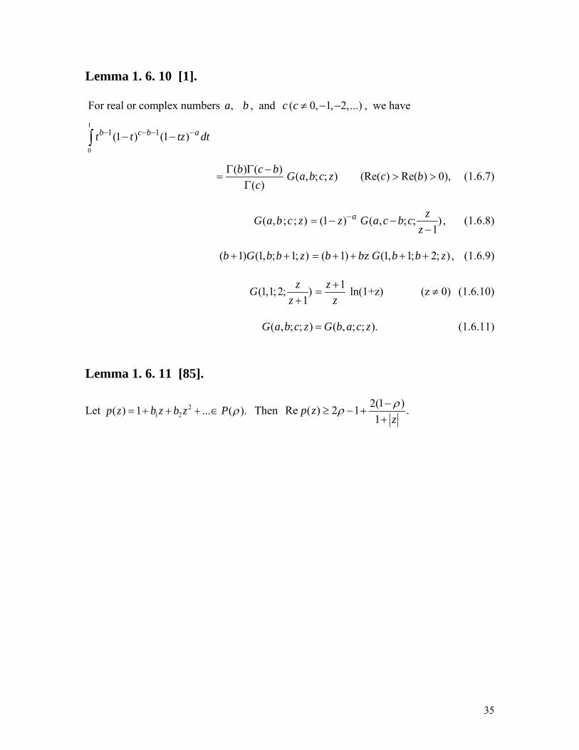
Lemma 1. 6. 10 [1].
For real or complex numbers ,a b , and ( 0, 1, 2,...)c c ≠ − − , we have 1
0
1 1(1 ) (1 )b c b at t tz dt− − − −− −∫
( ) ( ) ( , ; ; ) (Re( ) Re( ) 0),( )
b c b G a b c z c bc
Γ Γ −= > >
Γ (1.6.7)
( , ; ; ) (1 ) ( , ; ; ) ,1
a zG a b c z z G a c b cz
−= − −−
(1.6.8)
( 1) (1, ; 1; ) ( 1) z (1, 1; 2; ) ,b G b b z b b G b b z+ + = + + + + (1.6.9)
1(1,1;2; ) ln(1+z) (z 0)1
z zGz z
+= ≠
+ (1.6.10)
( , ; ; ) ( , ; ; ).G a b c z G b a c z= (1.6.11)
Lemma 1. 6. 11 [85].
Let 21 2( ) 1 ... ( ).p z b z b z P ρ= + + + ∈ Then 2(1 )Re ( ) 2 1 .
1p z
zρρ −
≥ − ++
36
CHAPTER 2
ON ANALYTIC FUNCTIONS WITH
GENERALIZED BOUNDED MOCANU
VARIATION
2.1 Introduction
It is well known [28] that a number of important classes of univalent functions (e.g.
convex, starlike) are related through their derivatives by functions with positive real part.
These functions play an important part in problem from signal theory, in moment
problems and in constructing quadrature formulas, see Ronning [97] and the references
cited therein for some recent applications. In this chapter, we introduce and consider
some new classes of functions by replacing functions with positive real part by certain
weighted differences of such functions.
In section 2.2, we define a new class ( , )kB α β for real α , 1 1,2
β−≤ < 2 and .k z E≥ ∈
For different choices of parameters ,k α and β we presents its relationships with the
previously known classes. It is known [113] that 2 ( , )B α β is a subclass of Bazilevic
functions defined in [7], and consists entirely of univalent functions. We study the
relationship between the classes ( , )kB α β and kR , where kR denotes the class of
bounded radius rotation, see [36]. In this section we focus on the inclusion results
between the classes ( , )kB α β and 1 1( , ).kB α β We also eastablish the criterion of
univlance for the class ( , )kB α β by restricting the parameter
2( 2 1) , 0.(1 )
k α αβ β αβ
+ − +≤ ≠
− As a special case, we deduce that 2 ( , )f B α β∈ is
univalent in 1for 0, 1.2
E α β−> ≤ <
37
In section 2.3, we derive arc lengths for the class ( , ).kB α β In addition, we characterize
the growth of the coefficient for the class ( , )kB α β by specializing the parameter 0.α >
In section 2.4, we have shown that the class (0, )kB β preserves the Barnardi integral
operator. Further we have discussed in details the sharp bounds of the class 2 ( , )B α β for
0α ≠ and 0 1,β< < by using the Gauss hypergeometric function. Finally, in this
section, for different parameters of interest we obtained the coefficient bounds by
assuming 2a to be real. We also derive a covering and distortion theorems for the classes
2 ( , )B α β and (1, )kB β by restricting the parameters ,k α and β . The contents of this
chapter have been published in the journal of Applied Mathematics and Computations,
see [76].
We now define the following class.
2.2 The class kB (α,β)
Definition 2. 2.1.
Let f ∈A with ( ) ( ) 0f z f zz′
≠ in E , and let
( ) ( )( , , , ( )) (1 ) 1 ,( ) (1 ) ( )
zf z zf zJ k f zf z f z
αα β α ββ
⎡ ⎤′ ′′⎧ ⎫= − + − +⎨ ⎬⎢ ⎥′− ⎩ ⎭⎣ ⎦
for real α and 1 1.2
β−≤ <
Then ( , )kf B α β∈ if and only if ( , , , ( )) for , 2.kJ k f z z E kα β Ρ∈ ∈ ≥
For any real α and 1 1,2
β−≤ < we note that the identity function belongs to ( , )kB α β so
that ( , )kB α β is not empty
.Special cases.
(i). For 22, 0 1, ( ,0)k Bα α= ≤ < is a subclass of A introduced by Mocanu
[60]. Also, see [57, 75].
38
(ii). It is well known [113] that 2 ( , )B α β is a subclass of Bazilevic functions
defined in [7]. Hence 2 ( , )B α β consists entirely of univalent functions.
(iii). (1,0)k kB V= is the well known class of functions of bounded boundary rotation.
(iv). (0, ) , wherek k kB R Rβ = denotes the class of bounded radius rotation, see[36].
(v). *2 2(1,0) , (0, ) ,B C B Sβ= = where *andC S are respectively the classes of
convex and starlike univalent functions in .E
2 .2. 1 Relation between the classes kB (α,β) and kR
Theorem 2.2.2.
Let ( , ), 0,kf B α β α∈ ≠ if and only if there is a function (0, )k kg B Rβ∈ =
such that 1
1
1
0
( )( ) ...,mz
m g tf z m t dt zt
αβ−
−⎡ ⎤
⎛ ⎞⎢ ⎥= = +⎜ ⎟⎢ ⎥⎝ ⎠⎣ ⎦∫
where (1 )(1 )1 .m α β
α− −
= +
Proof.
A simple computation yields
( ) ( ) ( )(1 ) 1 .( ) (1 ) ( ) ( )
zf z zf z zg zf z f z g z
αα ββ
′ ′′ ′⎛ ⎞− + − + =⎜ ⎟′− ⎝ ⎠
If the right hand side belongs to ,kP so does the left hand side and conversely. Theorem 2.2.3.
Let ( , ).kf B α β∈ Then the function
11( )( ) ( ( ))f zg z z f z
z
ααβ
−−⎛ ⎞ ′= ⎜ ⎟
⎝ ⎠ (2.2.1)
39
belongs to kR for all .z E∈ Proof. Differentiating (2.2.1) logarithmically, we have
( ) ( ) ( )(1 )( ) ( ) (1 ) ( )
zg z zf z zf zg z f z f z
αα αβ
′ ′ ′′⎛ ⎞= − + + ⎜ ⎟′− ⎝ ⎠
and result follows immediately since ( , ).kf B α β∈ Theorem 2.2.4.
( , ) , for 0, 0 1.kkB Rα β α β⊂ > ≤ <
Proof. Let
( ) ( ),( )
zf z p zf z′
=
( )p z is analytic in E with (0) 1.p = Now
1 ( ) ( ) 1(1 )(1 ) 1 ( ) ( ) , .1 ( ) ( ) 1 k
zf z zf z m p z zp z P z Ef z f z m
αα β α β ββ β⎡ ⎤′ ′′⎛ ⎞ ⎡ ⎤⎧ ⎫′− − + − + = + − ∈ ∈⎨ ⎬⎢ ⎥⎜ ⎟ ⎢ ⎥′− − ⎩ ⎭⎣ ⎦⎝ ⎠⎣ ⎦
This implies 1 ( )( )( ) k
zp zp z Pm p z
′⎧ ⎫+ ∈⎨ ⎬
⎩ ⎭ and , by Lemma 1.6.8, it follows that
, .kp P z E∈ ∈ This proves that kf R∈ in .E
2.2.2 Inclusion results between the classes kB (α,β) and 1k 1B (α ,β)
Theorem 2.2.5.
(i) 1 1 1( , ) ( , ), 0k kB Bα β α β α α⊂ < ≤ and 1
12 .k k α αα−⎛ ⎞= ⎜ ⎟
⎝ ⎠
40
(ii) 1 11
( , ) ( , ), 0 .k kB Bα β α β α α⊂ < ≤
Proof.
(i) Let ( , ).kf B α β∈ Then
1 1( ) ( )(1 )(1 ) 1( ) ( )
zf z zf zf z f z
α β α β′ ′′⎛ ⎞
− − + − +⎜ ⎟′⎝ ⎠
1 1(1 )( )( ) ( ) ( )(1 )(1 ) 1( ) ( ) ( )
zf z zf z zf zf z f z f z
α β α αα β α βα α⎡ ⎤′ ′′ ′⎛ ⎞ − −
= − − + − + −⎢ ⎥⎜ ⎟′⎝ ⎠⎣ ⎦
1 11 2 1 2(1 ) ( ) ( ) , , ,kh z h z h h Pα α αβ
α α−⎡ ⎤= − − ∈⎢ ⎥⎣ ⎦
(2.2.2)
by using Definition 2.2.1 and Theorem 2.2.4. From (2.2.2), it follows that
21 1
10
Re ( , , ( ))J f z d kπ α α αα β θ π
α α−⎛ ⎞≤ +⎜ ⎟
⎝ ⎠∫
12 .kα α πα−⎛ ⎞= ⎜ ⎟
⎝ ⎠
This completes the proof of (i).
(ii) Let ( , ).kf B α β∈ Then
11
( ) ( )(1 ) 1( ) (1 ) ( )
zf z zf zf z f z
αα ββ
′ ′′⎛ ⎞− + − +⎜ ⎟′− ⎝ ⎠
1 1( ) ( ) ( )(1 ) (1 ) 1( ) ( ) (1 ) ( )
zf z zf z zf zf z f z f z
α α αα α βα α β
⎡ ⎤′ ′ ′′⎛ ⎞= − + − + + − +⎢ ⎥⎜ ⎟′− ⎝ ⎠⎣ ⎦
1 11 2 1 2(1 ) ( ) ( ), , , ,kH z H z H H P z Eα α
α α= − + ∈ ∈
since kP is a convex set, see [70]. Therefore ( , ) for .f B z Ek α β∈ ∈
41
2.2.3 The condition of univalency for the class kB (α,β) Theorem 2.2.6.
Let ( , ).kf B α β∈ Then f is univalent in E for 2( 2 1) , 0.(1 )
k α αβ β αβ
+ − +≤ ≠
−
Proof.
Since ( , )kf B α β∈ we can write, for , 0 1, 0 2 ,1 2
iz re rθ θ θ π= ≤ < ≤ < ≤
2
1
(1 ) ( ) 1 ( ) 2Re 1 ( 1) .( ) (1 ) ( ) 2 1
zf z zf z kdf z f z
θ
θ
α π βθ πα β α β
⎧ ⎫′ ′′⎛ ⎞−+ + > − − +⎨ ⎬⎜ ⎟′− −⎝ ⎠⎩ ⎭
∫
2
1
( ) 1(1 ) ( ) 1Re 1 1 1 2 .( ) ( ) 2
zf z zf z kdf z f z
θ
θ
β ββ θ β πα α
⎡ ⎤′′ ′⎛ ⎞ ⎡ ⎤− −⎧ ⎫ ⎛ ⎞⎛ ⎞+ + + − > − − −⎨ ⎬⎢ ⎥⎜ ⎟ ⎜ ⎟⎜ ⎟⎢ ⎥′ ⎩ ⎭ ⎝ ⎠⎝ ⎠⎣ ⎦⎝ ⎠⎣ ⎦∫
This implies , by using Lemma 1.6.6, that f is univalent in E if
2( 2 1) .(1 )
k α αβ ββ
+ − +≤
−
As a special case, we deduce that 2 ( , )f B α β∈ is univalent in
1for 0, 1.2
E α β−> ≤ <
2.2 Arc length problems and growth of the coefficient for the
class kB (α,β)
Theorem 2.3.1.
Let ( , ),kf B α β∈ 0α > and ( )rL f denote the length of the curve
0 2, ( ),0 2 and ( ) max ( ) . Then,i iC C f re M r f reθ θ
θ πθ π
≤ ≤= ≤ ≤ = for 0 1.r< <
42
(i) { }( )( ) (1 ) 2 , 2.(1 )rM rL f k β β π α
β≤ − + ≥
−
(ii) { }( )( ) (1 )(2 ) 2 , 0 2.(1 )rM rL f k β α αβ π α
α β≤ − − + < <
−
Proof.
(i) With ,iz re θ=
2 2arg( ( ))
0 0
( ) ( ) ( ) .i zf zrL f zf z d zf z e d
π π
θ θ′−′ ′= =∫ ∫
Integration by parts gives us 2
0
arg( ( )) ( ( ))( ) ( ) Re( )r
i zf z zf zL f f z e df z
π
θ′− ′ ′⎧ ⎫= ⎨ ⎬′⎩ ⎭∫
2
0
( ) ( )Re ( , , ( )) ( 1)( ) 1
M r zf zJ f z df z
π αβα β α θα β
′≤ + − +
−∫
( ) 2( 1)1
M r k k αβπ α π πα β
⎡ ⎤≤ + − +⎢ ⎥−⎣ ⎦
2( ) .1
M r k βπβ
⎡ ⎤= +⎢ ⎥−⎣ ⎦
Proof of (ii) lies on similar lines. Theorem 2.3.2.
Let ,f given by (1.2.1), belongs to ( , )kB α β for 0.α > Then, for 2.n ≥
1(1) ( ),nnna O M
n−
=
where (1)O is a constant depending on ,α β and k only.
43
Proof.
Since 2
0
1 ( ) , ,2
in in nna zf z e d z re
r
πθ θθ
π−′= =∫
we have
2
0
1 1( ) ( ).2 2n rn nn a zf z d L f
r r
π
θπ π
′≤ =∫
Now using Theorem 2.3.1 with 11 ,rn
= − we prove the result.
2.4 Properties of the special classes of the class kB (α,β)
2.4.1 Integral preserving property of the class kB (0,β)
Theorem 2.4.1. Let, for 0,γ > F be defined as
1
0
1( ) ( ) ,z
F z t f t dtz
γγ
γ −+= ∫ (2.4.1)
and let (0, ).kf B β∈ Then (0, )kF B β∈ in .E Proof. Set
1 2( ) 1 1( ) ( ) ( ),
( ) 4 2 4 2zF z k kH z h z h zF z′ ⎛ ⎞ ⎛ ⎞= = + − −⎜ ⎟ ⎜ ⎟
⎝ ⎠ ⎝ ⎠
where ( )H z is analytic in E with (0) 1.H = Then from (2.4.1), we have
( ) ( )( ) , .( ) ( ) k
zf z zH zH z P z Ef z H z γ′ ′⎧ ⎫
= + ∈ ∈⎨ ⎬+⎩ ⎭
Now
44
( )( )( ) ( )( )
zH zH z H zH zγφ γ
′∗ = +
+
1 21 2
1 2
( ) ( )1 1( ) ( ) ,4 2 ( ) 4 2 ( )
zh z zh zk kh z h zh z h zγ γ
⎧ ⎫ ⎧ ⎫′ ′⎪ ⎪ ⎪ ⎪⎛ ⎞ ⎛ ⎞= + + − − +⎨ ⎬ ⎨ ⎬⎜ ⎟ ⎜ ⎟+ +⎝ ⎠ ⎝ ⎠⎪ ⎪ ⎪ ⎪⎩ ⎭ ⎩ ⎭
where
2
1( ) .1 (1 ) 1 (1 )
z zzz zγ
γφγ γ
= ++ − + −
It follows that ( )( ) , , 1, 2.( )
ii
i
zh zh z P z E ih z γ
⎧ ⎫′⎪ ⎪+ ∈ ∈ =⎨ ⎬+⎪ ⎪⎩ ⎭ We want to show that ih P∈ in
E which maps kH P∈ in .E We proceed by forming the functional ( , )u vΨ with
( ), ( ).i iu h z v zh z′= =
Thus
( , ) .vu v uu γ
Ψ = ++
The first two conditions of Lemma 1.6.7 are clearly satisfied. We verify the condition (iii) as follows.
12 1 2 2
2
Re ( , ) ,viu vuγ
γΨ =
+
and by putting
22
1(1 ) ,
2uv − +
≤
we have
22
2 1 2 22
(1 )Re ( , ) 0.2( )
uiu vu
γγ
− +Ψ ≤ ≤
+
This proves , 1, 2ih P i∈ = and the proof is complete.
45
2.4.2 Some Sharp bounds and distortion theorem for the
class 2B (α,β)
In the following, we study the distortion theorems for the class ),( βαkB with some
restrictions on α,k and β . We shall use the hypergeoemtric functions.
Let );,,( zcbaG be the analytic functions for z in E as defined by (1.6.7) that is
1
0
1 1( )( , , ; ) (1 ) (1 ) ,( ) ( )
a c a bcG a b c z u u zu dua c a
− − − −Γ= − −Γ Γ − ∫
where 0}Re{ >a and .0}Re{ >− ac In addition, we define the functions:
12(1 )( , , ) ( , , 1, ) ,mM r r G m m rβα β
α−⎡ ⎤= +⎢ ⎥⎣ ⎦
(2.4.2)
and
2(1 )
1
0
1
,( , , ) (1 )z
m i mf z m t e t dt
βθ α
θ α β− −
−⎡ ⎤= −⎢ ⎥⎣ ⎦∫ (2.4.3)
where (1 )(1 )1 , 0, 0 2 .m α β α θ π
α− −
= + ≠ ≤ ≤
We now prove the following. Theorem 2.4.2. Let 2 ( , ), 0, 0 1,f B α β α β∈ ≠ < < and (0 1).z r r= < < Then
(i) .0),,,()(),,( >≤≤− αβαβα forrMzfrM
(ii) .0),,,()(),,( <−≤≤ αβαβα forrMzfrM
This result is sharp and equality occurs, for the function ),,( zf βαθ , defined by (2.4.3),
with suitabaly chosen θ .
46
Proof. We consider 0>α and the case 0α < follows on similar lines.
From Theorem 3.3.1, for 2 ( , )f B α β∈ if and only if, there exists a ∗=∈ SRg 2 such that
1
0
11
,( )( )
zm
mg tf z m t dt
t
βα−
−⎡ ⎤⎛ ⎞⎢ ⎥= ⎜ ⎟⎢ ⎥⎝ ⎠⎢ ⎥⎣ ⎦
∫ (2.4.4)
where
(1 )(1 )1 , ( 0).m α β αα
− −= + >
We may take ,z r= for the general case can be reduced to this by considering the
function ( )f zzη with suitably chosen η such that 1η = . Taking z r= and integrating
along the positive real axis, we obtain from (2.4.4), for ,it e θρ=
1
( 1) 1
0
1
.( )( )
ri m m
mgf r me d
βα
θ ρρ ρρ
−
− −⎡ ⎤
⎛ ⎞⎢ ⎥= ⎜ ⎟⎢ ⎥⎝ ⎠⎢ ⎥⎣ ⎦∫ (2.4.5)
Since g is starlike, we have
2 2( ) .(1 ) (1 )
g tρ ρρ ρ
≤ ≤+ −
(2.4.6)
Using (2.4.6) in (2.4.5), we obtain 2(1 )
1
0
( ) (1 )r
m mf r m dβ
αρ ρ ρ− −
−≤ −∫
1 2(1 )
1
0
(1 ) , ( ).mmr u ru du ruβ
α ρ− −
−= − =∫ (2.4.7)
Therefore, .0),,,()( >≤ αβα forrMrf
47
To prove the left hand inequality, we consider the straight line *Γ joining 0 to
( ) .if z Re φ= *Γ is the image of a Jordan arc γ in E containing 0 and .iz re θ= Suppose
now 0z is a point on the circumference z r= such that
0 0 2( ) min ( ) .if z f re θ
θ π≤ ≤=
We consider .0>α From (2.4.5) and (2.4.6), we obtain
00
2(1 )1( ) (1 )
rm mf z m d
βαρ ρ ρ
− −−≥ +∫
1
0
2(1 )1(1 ) ,m mmr u ru du
βα
− −−= +∫
and this implies .0),,,()( >−≥ αβα rMzf
Using Definition 2.2.1 , relation (2.4.4) and Theorem 2.4.2, we have:
Theorem 2.4.3.
Let 2 ( , ), 0,f B α β α∈ > Then, for (0 1),z r r= < < we have
2 2
2 2
1 (1 ) ( ,0, ) 1 (1 ) ( ,0, )( ) .
(1 ) (1 )r r M r r r M r
f zr r r r
α α α αα α
+ − + − + − −′≤ ≤
+ −
This result is sharp.
2.4.3 Coefficient bounds and covering theorem for the
class 2B (α,β)
Theorem 2.4.4. Let 2 ( , ) 0 1, 0,f B α β β α∈ < < ≠ and be given by (3.1.1).
48
Then
22(1 ) .
(1 )(1 ) 2a β
α β α−
≤− − +
For the proof we can assume 2a to be real and make use of Theorem 3.3.9 (i) for
0>α .The case 0<α is similar. We can write
2 32(1 )( , , ) ( ),(1 )(1 ) 2
M r r r O rβα βα β α
−= + +
− − +
and
2 32( ) ( ).f r r a r O r= + +
Therefore, we have
22(1 ) , ( 0).
(1 )(1 ) 2a β α
α β α−
≤ >− − +
Theorem 2.4.5.
Let .121,0),,(2 <≤
−>∈ βαβαBf Then the disk E is mapped onto a domain that
contains the disk
[ ]0(1 )(1 ) 2 .
2 ( 2) ( 2)w α β α
α β α− − +
>+ + −
Proof. From Theorem 3.3.5, it follows that f is univalent in E . Let 0w be any complex number
such that 0)( wzf ≠ for .Ez∈ Then
...)1()(
)( 2
02
0
0 +++=−
zw
azzfw
zfw
is univalent and hence .21
02 ≤+
wa
Now, using Theorem 2.4.4, we obtain the required result.
49
2.4.4 A distortion theorem for the class kB (1,β)
Theorem 2.4.6. Let ).,1( βkBf ∈ Then, with ,
11, 1 r
rrrz+−
== we have
1 11
1 1 1 12 2( , , , 1) ( , , , ) ( ) ( , , , 1) ( , , , ) ,
b ba aG a b c r G a b c r f z G a b c r G a b c r
a a
− −− −⎡ ⎤ ⎡ ⎤− − − ≤ ≤ − − −⎣ ⎦ ⎣ ⎦
where
1)1(12
+−⎟⎠⎞
⎜⎝⎛ −= βka (2.4.8)
β2=b (2.4.9)
.2)1(12
+−⎟⎠⎞
⎜⎝⎛ −= βkc (2.4.10)
Proof.
Since ),,1( βkBf ∈ we can write from (2.4.6)
.,)()(1
kRgzzgzf ∈⎟⎠⎞
⎜⎝⎛=′
−β
Now, for ,kRg ∈ it is well-known [2] that
( )( )
( )( )
1 12 2
1 12 2
1 1( ) .
1 1
k k
k k
z zg z
z z
− −
+ +
− +≤ ≤
+ − (2.4.11)
Therefore, we have
( )( )
( 1)(1 )2
( 1)(1 )2
1( ) .
1
k
k
zf z
z
β
β
− −
+ −
−′ ≥
+
Let rd denote the radius of the largest schlicht disk centered at the origin contained in
the image of rz < under ).(zf Then there is a point ,, 00 rzz = such that
50
.)( 0 rdzf = The ray from 0 to )( 0zf lies entirely in the image and the inverse image of
this ray is a curve C in .rz < Now
∫ ′==C
r dzzfzfd )()( 0
( )( )
( 1)(1 )2
( 1)(1 )2
1
1
k
kC
zdz
z
β
β
− −
+ −
−≥
+∫
( )
( )
( 1)(1 )2
( 1)(1 )0 2
1
1
kz
k
sds
s
β
β
− −
+ −
−≥
+∫
( 1)(1 )
2
2(1 )0
11 (1 )
kz s ds
s s
β
β
− −
−
−⎛ ⎞= ⎜ ⎟+ +⎝ ⎠∫
11 2
( 1)(1 )2
1
1 2 1( )2 1 1
zz k st dt with t
t s
ββ
−+
− −− −⎛ ⎞≥ =⎜ ⎟+ +⎝ ⎠∫
1( 1)(1 )12 1 22( 2) (1 )
0
r krt t dt
ββ β−
− −+− −= − +∫
2 1( 1)(1 )1 222 (1 )
0
kt t dtβ
β β−− − −+ +∫
.1 2I I= +
Taking ,,11
11 urtrrr
==+− we have
11 1
1 1 10
( 2) (1 )b a a bI r u ru du− − −= − +∫
1
1 12 ( ) ( ) ( , , , ),
( )
ba a c ar G a b c r
a c
−⎛ ⎞− Γ Γ −= −⎜ ⎟ Γ⎝ ⎠
51
were cba ,, are given by (2.4.8), (2.4.9) and (2.4.10) respectively. We now calculate 2I .
1
1 12
0
2 (1 )b a bI t t dt− − −= +∫
12 ( ) ( ) ( , , , 1),
( )
b a c a G a b ca c
−⎛ ⎞ Γ Γ −= −⎜ ⎟ Γ⎝ ⎠
were cba ,, are given by (3.3.10), (3.3.11) and (3.3.12) respectively. This gives us the
lower bound.
Next we proceed to calculate the upper bound for )(zf .
( )( )
( 1)(1 )2
( 1)(1 )2
1( ) .
1
k
k
zf z
z
β
β
− −
+ −
+′ ≤
−
Therefore
( 1)(1 )2
( 1)(1 )2
0
(1 )( )(1 )
k
kz sf z ds
sβ
β
− −
− −+
≤−
∫
( 1)(1 )2
11
2 1 2
1
( 2) (1 )k
zz
dβ
β βξ ξ ξ− −
+−
− −≤ − +∫
1
11
2 ( , , , 1) ( , , , ) ,b
aG a b c r G a b c ra
−− −⎡ ⎤= − − −⎣ ⎦
were cba ,, are given by (2.4.8), (2.4.9) and (2.4.10) respectively. This completes the
proof.
52
CHAPTER 3
ON A CLASS OF P-VALENT BAZILEVIC
FUNCTIONS
3.1 Introduction
Loewner’s method [53] introduced in 1923 and developed by Kufarev in 1943 [39 ] was
to imbed an image domain in a continuously increasing family of domains and then
describe this family by a differential equation. Using the Loewner-Kufarev differential
equation Bazilevic [7] in 1955 was able to prove that the class of functions defined by
(1.4.8) is analytic and univalent in 1.z <
The class of Bazilevic functions has been extensively studied during the past fifty years
and significant contribution have been made in this fields, among others by Zamorski
[123 ], Pommerenke [88], Sheil-Small [101], Noor and Al-Bani [64], Thomas [114] and
Prokhorov [92].
In this chapter, we introduce a new subclass ,,В ( , , , )p a c A Bλ μα of analytic functions. The
class ,,В ( , , , )p a c A Bλ μα stem essentially from the class of Bazilevic functions. In this
chapter, we are primarily concerned with presenting some generalization and applications
of the class of P-valent Bazilevic functions. The results obtained generalize the related
works of some authors; see [45, 79, 91, 103, 121].
In section 3.2, we define the class ,,В ( , , , ),p a c A Bλ μα where 0, 0, 1 1,Bμ α> ≥ − ≤ ≤
, ,A B A pλ≠ ∈ > − and 0, \ {0, 1, 2, 3,...}.a c −∈ = − − −
We investigate a number of inclusion relationships for this class. Section 3.3 focuses on
some interesting properties of the subclass ,1,В ( , , , ).p a c A Bλα The most interesting one is
that the class ,1,В ( , , , )p a c A Bλα is closed under convolution and the generalized Livingston-
53
Libra-Bernardi operator defined by (1.5.5), see [43] belongs to this class. In addition, we
characterize the properties of the class of close-to-convex functions. Finally in
section 3.4, we establish distortion theorems for the class ,,В ( , , , )p a c A Bλ μα , the lower and
upper bounds of μλ
⎟⎟⎠
⎞⎜⎜⎝
⎛p
p
zzfcaI )(),(
Re for ,,( ) В ( , , , )pf z a c A Bλ μα∈ and some other
interesting properties of p-valent functions which are defined here by means of a certain
linear operator ( , ) ( ).pI a c f zλ
3.2 The class λ,μ
p,αВ (a,c, A, )B
Using the Cho-Kown-Srivastava operator ( , ),pI a cλ we now define a new subclass of
( )pA as follows.
Definition 3. 2.1.
Assume that 0, 0, 1 1, , ,B A B Aμ α> ≥ − ≤ ≤ ≠ ∈ we say that a function
( ) ( )f z p∈A is in the class ,,В ( , , , )p a c A Bλ μα if it satisfies:
where the powers are understood as principle values.
In particular, we let ,,В ( , ,1 2 , 1)p a cλ μα ρ− − ,
,В ( , , )p a cλ μα ρ≡ for 1 2 , 1A Bρ= − = − and
0 .pρ≤ < It is obvious that ,,В ( , , )pf a cλ μα ρ∈ if and only if ( )f p∈A satisfies
11`( , ) ( ) ( , ) ( ) ( , ) ( )
Re (1 ) , .p p pp p p
I a c f z I a c f z I a c f zz E
z z z
μ μλ λ λ
α α ρ−+⎧ ⎫⎛ ⎞ ⎛ ⎞⎛ ⎞⎪ ⎪− + > ∈⎜ ⎟ ⎜ ⎟⎜ ⎟⎨ ⎬⎜ ⎟ ⎜ ⎟⎜ ⎟
⎪ ⎪⎝ ⎠ ⎝ ⎠⎝ ⎠⎩ ⎭
11( , ) ( ) ( , ) ( ) ( , ) ( ) 1(1 ) , ,1
p p pp p p
I a c f z I a c f z I a c f z Az z Ez z z Bz
μ μλ λ λ
α α−+⎧ ⎫⎛ ⎞ ⎛ ⎞⎛ ⎞ +⎪ ⎪− + ∈⎜ ⎟ ⎜ ⎟⎜ ⎟⎨ ⎬⎜ ⎟ ⎜ ⎟⎜ ⎟ +⎪ ⎪⎝ ⎠ ⎝ ⎠⎝ ⎠⎩ ⎭≺
54
Special Cases.
(i) When 0,,, 1, 0, then В ( ,1, , )pa p c p A Bμαλ= = = is the class studied by Liu
[45].
(ii) The subclass 0,1,1В ( ,1,1, 1) В( )pμ μ− = has been discussed by Singh [102], see
also [79].
(iii) The subclass 0,,1В ( ,1, , ), 1 1,p p A B B A Bμ − ≤ < ≤ < was introduced by Yang
[121].
(iv) For the class 0,1,В ( ,1, ,0),p Aμ
α we refer [91].
Definition 3.2.2
A function (1)f ∈ ≡A A is said to be close-to-convex of order β in E if there are a
convex univalent function g ∈A and a real γ such that
( )Re for .( )i
f z z Ee g zγ β
′> − ∈
′
3. 2.1 Inclusion results for the class .λ,μp,αВ (a,c,A,B) of generalized
Bazilevic functions Theorem 3.2.3.
Let ,,0, ( ) В ( , , , )pf z a c A Bλ μαα > ∈ . Then
( , ) ( ) 1( ) ( ),
1p
p
I a c f z Azq z z Ez Bz
μλ⎛ ⎞ +∈⎜ ⎟⎜ ⎟ +⎝ ⎠
≺ ≺ (3.2.1)
1(1 )(1 ) (1, 1; 1; ), 0,
1( )
( )1 , 0.( )
A A p BzBz G BB B Bz
q zp Az B
p
λ μα
λ μλ μ α
− +⎧ + − + + ≠⎪ +⎪= ⎨ +⎪ + =⎪ + +⎩
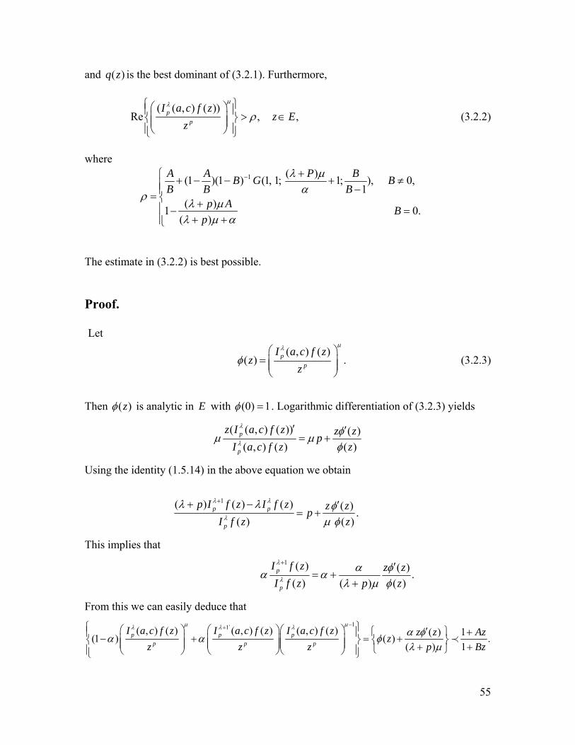
55
and ( )q z is the best dominant of (3.2.1). Furthermore,
( ( , ) ( ))Re , ,p
p
I a c f zz E
z
μλ
ρ⎧ ⎫⎛ ⎞⎪ ⎪ > ∈⎜ ⎟⎨ ⎬⎜ ⎟⎪ ⎪⎝ ⎠⎩ ⎭
(3.2.2)
where 1 ( )(1 )(1 ) (1, 1; 1; ), 0,
1( )1 0.
( )
A A P BB G BB B B
p A Bp
λ μαρ
λ μλ μ α
− +⎧ + − − + ≠⎪ −⎪= ⎨ +⎪ − =+ +⎪⎩
The estimate in (3.2.2) is best possible. Proof.
Let
( , ) ( )( ) .p
p
I a c f zz
z
μλ
φ⎛ ⎞
= ⎜ ⎟⎜ ⎟⎝ ⎠
(3.2.3)
Then ( )zφ is analytic in E with (0) 1φ = . Logarithmic differentiation of (3.2.3) yields
( ( , ) ( )) ( )( , ) ( ) ( )
p
p
z I a c f z z zpI a c f z z
λ
λ
φμ μφ
′ ′= +
Using the identity (1.5.14) in the above equation we obtain
1( ) ( ) ( ) ( ) .
( ) ( )p p
p
p I f z I f z z zpI f z z
λ λ
λ
λ λ φμ φ
++ − ′= +
This implies that
1 ( ) ( ) .
( ) ( ) ( )p
p
I f z z zI f z p z
λ
λ
α φα αλ μ φ
+ ′= +
+
From this we can easily deduce that 11`( , ) ( ) ( , ) ( ) ( , ) ( ) ( ) 1(1 ) ( ) .
( ) 1p p p
p p p
I a c f z I a c f z I a c f z z z Azzz z z p Bz
μ μλ λ λ α φα α φλ μ
−+⎧ ⎫⎛ ⎞ ⎛ ⎞⎛ ⎞ ′⎧ ⎫ +⎪ ⎪− + = +⎜ ⎟ ⎜ ⎟⎜ ⎟⎨ ⎬ ⎨ ⎬⎜ ⎟ ⎜ ⎟⎜ ⎟ + +⎩ ⎭⎪ ⎪⎝ ⎠ ⎝ ⎠⎝ ⎠⎩ ⎭≺
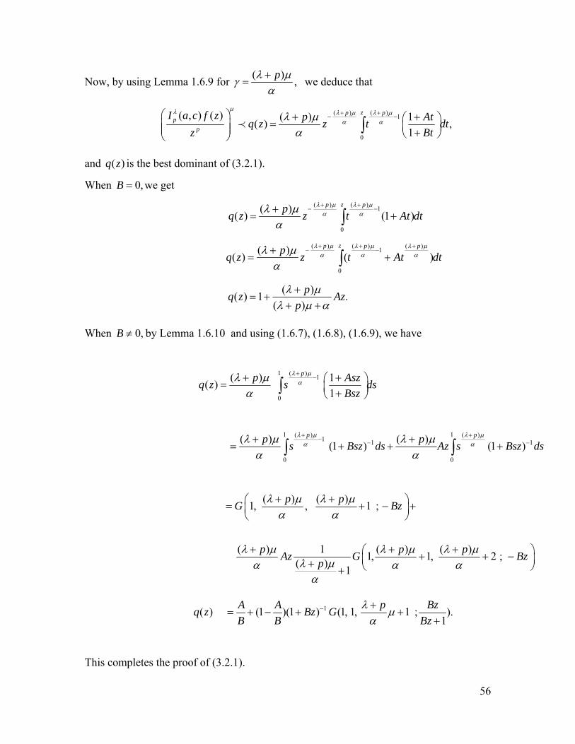
56
Now, by using Lemma 1.6.9 for ( ) ,pλ μγα+
= we deduce that
( ) ( ) 1
0
( , ) ( ) ( ) 1( ) ,1
zp pp
p
I a c f z p Atq z z t dtz Bt
μλ λ μ λ μα αλ μ
α
+ +− −⎛ ⎞ + +⎛ ⎞=⎜ ⎟ ⎜ ⎟⎜ ⎟ +⎝ ⎠⎝ ⎠
∫≺
and ( )q z is the best dominant of (3.2.1).
When 0,B = we get
( ) ( ) 1
0
( )( ) (1 )zp ppq z z t At dt
λ μ λ μα αλ μ
α
+ +− −+
= +∫
( ) ( ) ( )1
0
( )( ) ( )zp p ppq z z t At dt
λ μ λ μ λ μα α αλ μ
α
+ + +− −+
= +∫
( )( ) 1 .( )
pq z Azp
λ μλ μ α
+= +
+ +
When 0,B ≠ by Lemma 1.6.10 and using (1.6.7), (1.6.8), (1.6.9), we have
1 ( ) 1
0
( ) 1( )1
pp Aszq z s dsBsz
λ μαλ μ
α
+−+ +⎛ ⎞= ⎜ ⎟+⎝ ⎠∫
1 1( ) ( )1 1 1
0 0
( ) ( )(1 ) (1 )p pp ps Bsz ds Az s Bsz ds
λ μ λ μα αλ μ λ μ
α α
+ +− − −+ +
= + + +∫ ∫
( ) ( )1, , 1 ;
( ) 1 ( ) ( )1, 1, 2 ;( ) 1
p pG Bz
p p pAz G Bzp
λ μ λ μα α
λ μ λ μ λ μλ μα α α
α
+ +⎛ ⎞= + − +⎜ ⎟⎝ ⎠
+ + +⎛ ⎞+ + −⎜ ⎟+ ⎝ ⎠+
( )q z 1(1 )(1 ) (1, 1, 1 ; ).1
A A p BzBz GB B Bz
λ μα
− += + − + +
+
This completes the proof of (3.2.1).
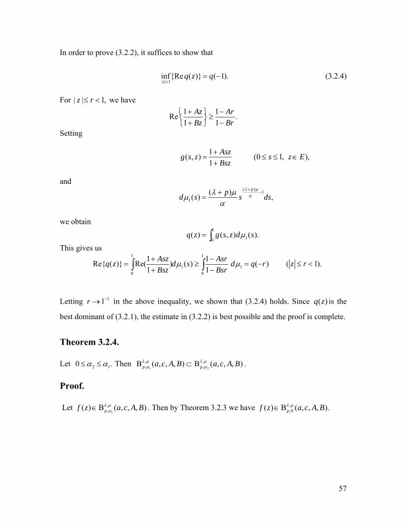
57
In order to prove (3.2.2), it suffices to show that
| | 1inf{Re ( )} ( 1).z
q z q<
= − (3.2.4)
For | | 1,z r≤ < we have
1 1Re .1 1
Az ArBz Br
+ −⎧ ⎫ ≥⎨ ⎬+ −⎩ ⎭
Setting
1( , ) (0 1, ),1
Aszg s z s z EBsz
+= ≤ ≤ ∈
+
and
( ) 1
1( )( ) ,
ppd s s dsλ μ
αλ μμα
+−+
=
we obtain
1
10( ) ( , ) ( ).q z g s z d sμ= ∫
This gives us
1 1
1 10 0
1 1Re{ ( )} Re( ) ( ) ( ) ( 1).1 1
Asz Asrq z d s d q r z rBsz Bsr
μ μ+ −= ≥ = − ≤ <
+ −∫ ∫
Letting 11r −→ in the above inequality, we shown that (3.2.4) holds. Since ( )q z is the
best dominant of (3.2.1), the estimate in (3.2.2) is best possible and the proof is complete.
Theorem 3.2.4.
Let 2 10 .α α≤ ≤ Then 1
,,В ( , , , )p a c A Bλ μα ⊂
2
,,В ( , , , )p a c A Bλ μα .
Proof.
Let 1
,,( ) В ( , , , )pf z a c A Bλ μα∈ . Then by Theorem 3.2.3 we have ,
,0( ) В ( , , , ).pf z a c A Bλ μ∈
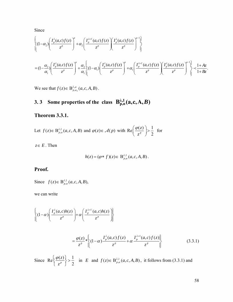
58
Since 11̀
2 2
1̀2 2
1 11 1
( , ) ( ) ( , ) ( ) ( , ) ( )(1 )
( , ) ( ) ( , ) ( ) ( , ) ( ) ( , ) ( )(1 ) (1 )
p p pp p p
p p p pp p p p
I a c f z I a c f z I a c f zz z z
I a c f z I a c f z I a c f z I a c f zz z z z
μ μλ λ λ
μ μλ λ λ λ
α α
α α α αα α
−+
+
⎧ ⎫⎛ ⎞ ⎛ ⎞⎛ ⎞⎪ ⎪− +⎜ ⎟ ⎜ ⎟⎜ ⎟⎨ ⎬⎜ ⎟ ⎜ ⎟⎜ ⎟⎪ ⎪⎝ ⎠ ⎝ ⎠⎝ ⎠⎩ ⎭
⎛ ⎞ ⎛ ⎞ ⎛ ⎞= − + − +⎜ ⎟ ⎜ ⎟ ⎜ ⎟⎜ ⎟ ⎜ ⎟ ⎜ ⎟
⎝ ⎠ ⎝ ⎠ ⎝ ⎠
11 .1
AzBz
μ−⎧ ⎫⎛ ⎞ +⎪ ⎪⎜ ⎟⎨ ⎬⎜ ⎟ +⎪ ⎪⎝ ⎠⎩ ⎭
≺
We see that2
,,( ) В ( , , , )pf z a c A Bλ μα∈ .
3. 3 Some properties of the class λ,1
p,αВ (a,c,A, )B Theorem 3.3.1.
Let ,1,( ) В ( , , , )pf z a c A Bλα∈ and ( ) ( )z pϕ ∈A with ( ) 1Re
2p
zz
ϕ⎛ ⎞ >⎜ ⎟⎝ ⎠
for
z E∈ . Then
( ) ( )( )h z f zϕ= ∗ ∈ ,1,В ( , , , )p a c A Bλα .
Proof.
Since ,1,( ) В ( , , , ),pf z a c A Bλα∈
we can write
1`( , ) ( ) ( , ) ( )
(1 ) p pp p
I a c h z I a c h zz z
λ λ
α α+⎧ ⎫⎛ ⎞ ⎛ ⎞⎪ ⎪− +⎜ ⎟ ⎜ ⎟⎨ ⎬⎜ ⎟ ⎜ ⎟⎪ ⎪⎝ ⎠ ⎝ ⎠⎩ ⎭
1( , ) ( ) ( , ) ( )( ) * (1 ) p pp p p
I a c f z I a c f zzz z z
λ λϕ α α+⎧ ⎫⎪ ⎪= − +⎨ ⎬
⎪ ⎪⎩ ⎭ (3.3.1)
Since ( ) 1Re2p
zz
ϕ⎧ ⎫ >⎨ ⎬⎩ ⎭
in E and ,1,( ) В ( , , , )pf z a c A Bλα∈ , it follows from (3.3.1) and
59
Lemma 1.6.6 that ( ) ( )( )h z f zϕ= ∗ ∈ ,,В ( , , , )p a c A Bλ μα . This completes the proof of
Theorem 3.3.1.
Theorem 3.3.2.
Let 0α > and ,1,( ) В ( , , , ).pf z a c A Bλα∈ Then
1 1
1 ( ) 1
0
( , ) ( ) 1Re ( ) ( ) ( 1).1
pm mp
p
I a c f z p Auu du mz Bu
λ λαλ
α
+−
⎛ ⎞⎛ ⎞ ⎛ ⎞+ −⎜ ⎟ > ≥⎜ ⎟ ⎜ ⎟⎜ ⎟⎜ ⎟ −⎝ ⎠⎝ ⎠⎜ ⎟
⎝ ⎠∫ (3.3.2)
This result is sharp.
Proof.
Let
1
( , ) ( )( ) p
p
I a c f zz
z
λ
φ = . (3.3.3)
Then the function 1 1( ) 1 ...z b zφ = + + is analytic in E . By making use of the identity
(1.5.14) and (3.3.3), we obtain
1`
1 1
( , ) ( ) ( , ) ( ) 1(1 ) ( ) ( ) ( ).( ) 1
p pp p
I a c f z I a c f z Azz z z z Ez z p Bz
λ λ αα α φ φλ
+⎧ ⎫⎛ ⎞ ⎛ ⎞ ⎧ ⎫ +⎪ ⎪ ′− + = + ∈⎜ ⎟ ⎜ ⎟⎨ ⎬ ⎨ ⎬⎜ ⎟ ⎜ ⎟ + +⎩ ⎭⎪ ⎪⎝ ⎠ ⎝ ⎠⎩ ⎭≺
Now by an application of Lemma 1.6.10, we get
1( ) ( ) 1
10
( ) 1( )1
p pP Atz z t dtBt
λ λα αλφ
α
+ +− −+ +⎛ ⎞ ⎜ ⎟+⎝ ⎠∫≺ .
This is equivalent to
1 ( ) 1
0
( , ) ( ) ( ) 1 ( )( ) ,1 ( )
pp
p
I a c f z p Auw zu duz Buw z
λ λαλ
α
+−+ +
=+∫ (3.3.4)
where ( )w z is analytic in E with (0) 0w = and| ( ) | 1 ( )w z z E< ∈ .
60
In view of 1 1B A− ≤ < ≤ and 0pλ + > it follows from (3.3.4) that
( , ) ( )Re p
p
I a c f zz
λ⎛ ⎞=⎜ ⎟⎜ ⎟
⎝ ⎠
1 ( ) 1
0
( ) 1 ( )Re( )1 ( )
pp Auw zu duBuw z
λαλ
α
+−+ +
+∫
1 ( ) 1
0
( ) 1( ) ( ).1
pp Auu du z EBu
λαλ
α
+−+ −
> ∈−∫ (3.3.5)
Therefore, with the aid of elementary inequality 1/ 1/Re( ) Re( )m mw w≥ for Re 0w > and
1,m ≥ the inequality (3.3.2) follows directly from (3.3.5).
To show the sharpness of (3.3.2), we consider the function 0 ( ) ( )f z p∈A defined by
1 ( ) 10
0
( , ) ( ) ( ) 1( ) .1
pp
p
I a c f z p Auzu duz Buz
λ λαλ
α
+−+ +
=+∫
For this function, we find that
1`0 0( , ) ( ) ( , ) ( ) 1(1 ) ( ),
1p p
p p
I a c f z I a c f z Az z Ez z Bz
λ λ
α α+⎧ ⎫⎛ ⎞ ⎛ ⎞ +⎪ ⎪− + = ∈⎜ ⎟ ⎜ ⎟⎨ ⎬⎜ ⎟ ⎜ ⎟ +⎪ ⎪⎝ ⎠ ⎝ ⎠⎩ ⎭
and
( ) 110
0
( , ) ( ) ( ) 1( ) ,1
pp
p
I a c f z p Auu duz Bu
λ λαλ
α
+−+ −
→−∫
as 1.z → − Hence the proof of the theorem is complete.
Theorem 3.3.3.
,1 ,1,0 , ,1( ) В ( , , , ) ( )( ) В ( , , , ),p p pf z a c A B f z a c A Bλ λ
λ∈ ⇔ ∈F where , pλF is the integral operator
defined by (1.5.5).
61
Proof.
Using identity (1.5.6) and
1( ( , ) ( )( )) ( ) ( , ) ( )( ) ( , ) ( )( ),p p pz I a c f z p I a c f z I a c f zλ λ λ
δ δ δλ λ+′ = + −,p ,p ,pF F F
for δ λ= , we deduce that
1( , ) ( ) ( , ) ( )( ),p p
a c f z a c f zz z
λ λλ
+⎛ ⎞ ⎛ ⎞=⎜ ⎟ ⎜ ⎟⎜ ⎟ ⎜ ⎟
⎝ ⎠ ⎝ ⎠
p p ,pI I F
and by using the definition of the class ,,В ( , , , )p a c A Bλ μα , the assertion of the Theorem
3.3.3 follows at once.
Theorem 3.3.4.
If ( ) ( ),f z p∈A then (i) ( ) ( ) ( )1 1 1( 1, ) ( ) ( , ) ( ) ( 1, ) ( ) .p p p
p p pz z I a c f z a z I a c f z a z I a c f zλ λ λ− − −′′ ′ ′+ = − + (3.3.6) . (ii) If 1 ( 1, ) ( )p
pz I a c f zλ− + is a convex univalent function, then 1 ( , ) ( )ppz I a c f zλ− is
close-to-convex of order 1aa− with respect to 1 ( 1, ) ( )p
pz I a c f zλ− + .
Proof.
(i) First we note that from the identity (1.5.15) we have
( ( 1, ) ( )) (1 ) ( 1, ) ( )p pz I a c f z p I a c f zλ λ′+ + − + =
( , ) ( ) (1 ) ( 1, ) ( ).p paI a c f z a I a c f zλ λ+ − + (3.3.7)
Since left hand side of (3.3.7) is equal to 1( ( 1, ) ( )) ,p
pz z I a c f zλ− ′+ we have
1 1 1( ( 1, ) ( )) ( ( , ) ( )) (1 )( ( 1, ) ( )).p p p
p p pz z I a c f z a z I a c f z a z I a c f zλ λ λ− − −′+ = + − + (3.3.8)
62
Differentiating both sides of (3.3.8) we obtain (3.3.6).
(ii) From (3.3.6) we conclude that
1 1
1 1
( ( , ) ( )) ( ( 1, ) ( ))1 1( ( 1, ) ( )) ( ( 1, ) ( ))
p pp p
p pp p
z I a c f z z I a c f zz
z I a c f z a z I a c f z
λ λ
λ λ
− −
− −
′ ′′+ = +
′ ′+ +.
1 1
1 1
( ( , ) ( )) ( ( 1, ) ( ))1Re Re 1( ( 1, ) ( )) ( ( 1, ) ( ))
p pp p
p pp p
z I a c f z z I a c f zz
z I a c f z a z I a c f z
λ λ
λ λ
− −
− −
⎡ ⎤ ⎡ ⎤′ ′′+ = +⎢ ⎥ ⎢ ⎥′ ′+ +⎢ ⎥ ⎢ ⎥⎣ ⎦ ⎣ ⎦
.
1 1Re(1 ) .aa a
−> − =
and by Definition 3.2.2, we obtain our required result.
3. 4 Sharp bounds and distortion theorems for the
class λ,μp,αВ (a,c,A, )B .
Theorem 3.4.1.
Let 0, 1 1, and ( )B f zα > − ≤ < ∈ ,,В ( , , , )p a c A Bλ μα .
(i) If ,A B> then
1 ( ) 1
0
( , ) ( ) ( ) 1Re , .1
pp
p
I a c f z p Au u du z Ez Bu
μλ λ μαλ μ
α
+−⎧ ⎫⎛ ⎞ + −⎪ ⎪ > ∈⎜ ⎟⎨ ⎬⎜ ⎟ −⎪ ⎪⎝ ⎠⎩ ⎭
∫ (3.4.1)
(ii) If ,A B< then
1 ( ) 1
0
( , ) ( ) ( ) 1Re , ,1
pp
p
I a c f z p Au u du z Ez Bu
μλ λ μαλ μ
α
+−⎧ ⎫⎛ ⎞ + −⎪ ⎪ < ∈⎜ ⎟⎨ ⎬⎜ ⎟ −⎪ ⎪⎝ ⎠⎩ ⎭
∫ (3.4.2)
63
and the inequalities are sharp with the extremal function defined by
, , ,( , ) ( ) pp A BI a c f z zλ
α μ =1/1 ( ) 1
0
( ) 1 .1
pp Auz u duBuz
μλ μαλ μ
α
+−⎧ ⎫+ +
⎨ ⎬+⎩ ⎭∫ (3.4.3)
Proof.
(i) Since ,,( ) В ( , , , )pf z a c A Bλ μα∈ , according to Theorem 3.2.3 we have
1 ( ) 1
0
( , ) ( ) ( ) 11
pp
p
I a c f z p Azu u duz Bzu
μλ λ μαλ μ
α
+−⎛ ⎞ + +
⎜ ⎟⎜ ⎟ +⎝ ⎠∫≺ .
Therefore it follows from the definition of subordination and A B> that
1 ( ) 1min
0
( , ) ( ) ( ) 1Re Re1
pp
z Ep
I a c f z p Azu u duz Bzu
μλ λ μαλ μ
α
+−
∈
⎧ ⎫⎛ ⎞ ⎧ ⎫+ +⎪ ⎪ ≥ ⎜ ⎟⎨ ⎬ ⎨ ⎬⎜ ⎟ +⎩ ⎭⎪ ⎪⎝ ⎠⎩ ⎭∫
1 ( ) 1
0
( ) 1min Re1
p
z E
p Azu u duBzu
λ μαλ μ
α
+−
∈
+ +⎧ ⎫= ⎨ ⎬+⎩ ⎭∫
1 ( ) 1
0
( ) 1 ,1
pp Au u du z EBu
λ μαλ μ
α
+−+ −
> ∈−∫ .
(ii) If ,A B< then
1 ( ) 1max
0
( , ) ( ) ( ) 1Re Re1
pp
z Ep
I a c f z p Azu u duz Bzu
μλ λ μαλ μ
α
+−
∈
⎧ ⎫⎛ ⎞ ⎧ ⎫+ +⎪ ⎪ ≤ ⎜ ⎟⎨ ⎬ ⎨ ⎬⎜ ⎟ +⎩ ⎭⎪ ⎪⎝ ⎠⎩ ⎭∫
1 ( ) 1
0
( ) 1max Re1
p
z E
p Azu u duBzu
λ μαλ μ
α
+−
∈
+ +⎧ ⎫= ⎨ ⎬+⎩ ⎭∫
64
1 ( ) 1
0
( ) 1 ,1
pp Au u du z EBu
λ μαλ μ
α
+−+ −
< ∈−∫ .
Noting that the function defined by (3.4.3) belongs to the class ,,В ( , , , )p a c A Bλ μα , we obtain
that the inequalities (3.4.1) and (3.4.2) are sharp.
By applying the similar techniques that we used in proving Theorem 3.4.1, we have the
following result.
Theorem 3. 4. 2.
Let 0, 1 1, and ( )A B f zα > − ≤ < ≤ ∈ ,,В ( , , , ).p a c A Bλ μα Then
1 ( ) 1
0
( , ) ( )( ) 1 Re1
pp
p
I a c f zp Au u duBu z
λλ μαλ μ
α
+− ⎧ ⎫+ + ⎪ ⎪< ⎨ ⎬+ ⎪ ⎪⎩ ⎭
∫
1 ( ) 1
0
( ) 1 , ,1
pp Au u du z EBu
λ μαλ μ
α
+−+ −
< ∈−∫ (3.4.4)
and inequality (3.4.4) is sharp with the extremal function defined by (3.4.3).
Proof.
Since ,,( ) В ( , , , )pf z a c A Bλ μα∈ , according to Theorem 3.2.3 we have
1 ( ) 1
0
( , ) ( ) ( ) 11
pp
p
I a c f z p Azu u duz Bzu
μλ λ μαλ μ
α
+−⎛ ⎞ + +
⎜ ⎟⎜ ⎟ +⎝ ⎠∫≺ .
Therefore it follows from the definition of subordination and B A> that
1 ( ) 1max
0
( , ) ( ) ( ) 1Re Re1
pp
z Ep
I a c f z p Azu u duz Bzu
μλ λ μαλ μ
α
+−
∈
⎧ ⎫⎛ ⎞ ⎧ ⎫+ +⎪ ⎪ ≤ ⎜ ⎟⎨ ⎬ ⎨ ⎬⎜ ⎟ +⎩ ⎭⎪ ⎪⎝ ⎠⎩ ⎭∫
1 ( ) 1
0
( ) 1max Re1
p
z E
p Azu u duBzu
λ μαλ μ
α
+−
∈
+ +⎧ ⎫= ⎨ ⎬+⎩ ⎭∫
65
1 ( ) 1
0
( ) 1 ,1
pp Au u du z EBu
λ μαλ μ
α
+−+ −
< ∈−∫
Also,
1 ( ) 1min
0
( , ) ( ) ( ) 1Re Re1
pp
z Ep
I a c f z p Azu u duz Bzu
μλ λ μαλ μ
α
+−
∈
⎧ ⎫⎛ ⎞ ⎧ ⎫+ +⎪ ⎪ ≥ ⎜ ⎟⎨ ⎬ ⎨ ⎬⎜ ⎟ +⎩ ⎭⎪ ⎪⎝ ⎠⎩ ⎭∫
1 ( ) 1
0
( ) 1min Re1
p
z E
p Azu u duBzu
λ μαλ μ
α
+−
∈
+ +⎧ ⎫= ⎨ ⎬+⎩ ⎭∫
1 ( ) 1
0
( ) 1 ,1
pp Au u du z EBu
λ μαλ μ
α
+−+ +
> ∈+∫
Theorem 3.4.3.
Let ,,( ) В ( , , , )pf z a c A Bλ μα∈ , 1 1.B A− ≤ < ≤
(i) If 0α = , then for 1,z r= < we have
1/ 1/1 1( , ) ( ) .
1 1p p
pAr Arr I a c f z rBr Br
μ μλ− +⎛ ⎞ ⎛ ⎞≤ ≤⎜ ⎟ ⎜ ⎟− +⎝ ⎠ ⎝ ⎠
(3.4.5)
and inequality (3.4.5) is sharp , with the extremal function defined by
1
1( , ) ( ) .1
pp
AzI a c f z zBz
μλ +⎛ ⎞= ⎜ ⎟+⎝ ⎠ (3.4.6)
(ii) If 0,α > then for 1,z r= < we have
66
1/1 ( ) 1
0
( ) 1 ( , ) ( )1
pp
pp Aurr u du I a c f z
Bur
μλ μλαλ μ
α
+−⎛ ⎞+ −
≤⎜ ⎟−⎝ ⎠∫
1/1 ( ) 1
0
( ) 1 ,1
pp p Aurr u du
Bur
μλ μαλ μ
α
+−⎛ ⎞+ +
≤ ⎜ ⎟+⎝ ⎠∫ (3.4.7)
and the inequality (3.4.7) is sharp with the extremal function defined by (3.4.3).
Proof.
(i) With 0α = . ,,0( ) В ( , , , ),pf z a c A Bλ μ∈ 1 1,B A− ≤ < ≤ we obtain from the definition
of ,, ( , , , )pB a c A Bλ μα that
( , ) ( ) 1 .1
pp
I a c f z Azz Bz
μλ⎛ ⎞ +⎜ ⎟⎜ ⎟ +⎝ ⎠
≺
According to the definition of the subordination, there exists an analytic function ( )w z in
E which satisfies ( )w z z≤ such that
( , ) ( ) 1 ( ) .1 ( )
pp
I a c f z Aw zz Bw z
μλ⎛ ⎞ +=⎜ ⎟⎜ ⎟ +⎝ ⎠
By applying Schwarz Lemma, we can write
2
1 2( ) ...w z c z c z= + +
with
( ) ,w z z≤ so that 1,z r= <
and therefore,
( , ) ( ) 1 ( )1 ( ) 1 ,1 ( ) 1 ( ) 1
pp
I a c f z A w zAw z Arz Bw z B w z Br
μλ⎛ ⎞ ++ += ≤ ≤⎜ ⎟⎜ ⎟ + + +⎝ ⎠
and
( , ) ( ) ( , ) ( ) 1Re .1
p pp p
I a c f z I a c f z Arz z Br
μ μλ λ⎛ ⎞ −≥ ≥⎜ ⎟⎜ ⎟ −⎝ ⎠
67
Hence
1/ 1/1 1( , ) ( )
1 1p p
pAr Arr I a c f z rBr Br
μ μλ− +⎛ ⎞ ⎛ ⎞≤ ≤⎜ ⎟ ⎜ ⎟− +⎝ ⎠ ⎝ ⎠
.
(ii) Let 0.α > Then by Theorem 3.2.3 we have,
1 ( ) 1
0
( , ) ( ) ( ) 1 .1
pp
p
I a c f z p Azu u duz Bzu
μλ λ μαλ μ
α
+−⎛ ⎞ + +
⎜ ⎟⎜ ⎟ +⎝ ⎠∫≺
Therefore it follows from the definition of subordination that
where 2
1 2( ) ...w z c z c z= + + is analytic in E and ( ) ,w z z≤ so when 1,z r= < we have
1 ( ) 1
0
( , ) ( ) ( ) 1 ( )1 ( )
pp
p
I a c f z p Auw z u duz Buw z
μλ λ μαλ μ
α
+−+ +
=+∫
1 1( ) ( )1 1
0 0
1 ( )( ) ( ) 1 ,1 ( ) 1
p pAu w zp p Auru du u duBu w z Bur
λ μ λ μα αλ μ λ μ
α α
+ +− −++ + +
≤ ≤ + +∫ ∫
and
1 1
0
( , ) ( ) ( , ) ( ) ( ) 1Re .1
pp p
p p
I a c f z I a c f z p Aur u duz z Bur
μ μ λλ λ μαλ μ
α
+⎛ ⎞ −⎜ ⎟⎝ ⎠
⎧ ⎫ + −⎪ ⎪≥ ≥⎨ ⎬ −⎪ ⎪⎩ ⎭∫
Hence
1 1
0
( , ) ( ) ( ) 1 ( ) ,1 ( )
pp
p
I a c f z p Auw z u duz Buw z
μ λλ μαλ μ
α
+⎛ ⎞ −⎜ ⎟⎝ ⎠
⎛ ⎞ + +=⎜ ⎟⎜ ⎟ +⎝ ⎠
∫
68
1/1 1
0
( ) 1 ( , ) ( )1
pp
pp Aurr u du I a c f z
Bur
μλ μλαλ μ
α
+⎛ ⎞ −⎜ ⎟⎝ ⎠
⎛ ⎞+ −≤⎜ ⎟⎜ ⎟−⎝ ⎠
∫
1/
1 1
0
( ) 1 .1
pp p Aurr u du
Bur
μλ μαλ μ
α
+⎛ ⎞ −⎜ ⎟⎝ ⎠
⎛ ⎞+ +≤ ⎜ ⎟⎜ ⎟+⎝ ⎠
∫
Note that the function defined by (3.4.3) belongs to ,
,В ( , , , )p a c A Bλ μα , we obtain that
the inequalities (3.4.5) and (3.4.6) are sharp.
By applying the same method as in Theorem 3.4.3, we have the following theorem.
Theorem 3.4.4.
Let ,,( ) В ( , , , )pf z a c A Bλ μα∈ , 1 1.A B− ≤ < ≤
(i). If 0α = , then for 1,z r= < we have
1/ 1/1 1( , ) ( ) .
1 1p p
pAr Arr I a c f z rBr Br
μ μλ+ −⎛ ⎞ ⎛ ⎞≤ ≤⎜ ⎟ ⎜ ⎟+ −⎝ ⎠ ⎝ ⎠
(3.4.8)
and the inequality (3.4.8) is sharp, with the extremal function defined by (3.4.6).
(ii). If 0,α > then for 1,z r= < we have
1/
1 1
0
( ) 1 ( , ) ( )1
pp
pp Aurr u du I a c f z
Bur
μλ μλαλ μ
α
+⎛ ⎞ −⎜ ⎟⎝ ⎠
⎛ ⎞+ +≤⎜ ⎟⎜ ⎟+⎝ ⎠
∫
1/
1 1
0
( ) 11
pp p Aurr u du
Bur
μλ μαλ μ
α
+⎛ ⎞ −⎜ ⎟⎝ ⎠
⎛ ⎞+ −≤ ⎜ ⎟⎜ ⎟−⎝ ⎠
∫ . (3.4.9)
and the inequality (3.4.9) is sharp with the extremal function as defined by (3.4.3).
69
Proof.
(i) If 0α = . Since ,,( ) В ( , , , )pf z a c A Bλ μα∈ , 1 1,A B− ≤ < ≤ we obtain from the
definition of ,,В ( , , , )p a c A Bλ μα that
( , ) ( ) 1 .1
pp
I a c f z Azz Bz
μλ⎛ ⎞ +⎜ ⎟⎜ ⎟ +⎝ ⎠
≺
According to the definition of the subordination, there exists an analytic function ( )w z in
E which satisfies ( )w z z≤ such that
( , ) ( ) 1 ( ) .1 ( )
pp
I a c f z Aw zz Bw z
μλ⎛ ⎞ +=⎜ ⎟⎜ ⎟ +⎝ ⎠
By applying Schwarz Lemma, we obtain that
2
1 2( ) ...w z c z c z= + +
( ) ,w z z≤ so that 1,z r= < we have
( , ) ( ) 1 ( )1 ( ) 1 ,1 ( ) 1 ( ) 1
pp
I a c f z A w zAw z Arz Bw z B w z Br
μλ⎛ ⎞ −+ −= ≤ ≤⎜ ⎟⎜ ⎟ + − −⎝ ⎠
and
( , ) ( ) ( , ) ( ) 1Re .1
p pp p
I a c f z I a c f z Arz z Br
μ μλ λ⎛ ⎞ +≥ ≥⎜ ⎟⎜ ⎟ +⎝ ⎠
Hence
1/ 1/1 1( , ) ( )
1 1p p
pAr Arr I a c f z rBr Br
μ μλ− +⎛ ⎞ ⎛ ⎞≤ ≤⎜ ⎟ ⎜ ⎟− +⎝ ⎠ ⎝ ⎠
.
(ii) Let 0.α > Then from Theorem 3.2.3 it follows that
1 ( ) 1
0
( , ) ( ) ( ) 1 .1
pp
p
I a c f z p Azu u duz Bzu
μλ λ μαλ μ
α
+−⎛ ⎞ + +
⎜ ⎟⎜ ⎟ +⎝ ⎠∫≺
and subordination yields
70
where 2
1 2( ) ...w z c z c z= + + is analytic in E and ( ) .w z z≤ So when 1,z r= < we have
1 ( ) 1
0
( , ) ( ) ( ) 1 ( )1 ( )
pp
p
I a c f z p Auw z u duz Buw z
μλ λ μαλ μ
α
+−+ +
=+∫
1 1( ) ( )1 1
0 0
1 ( )( ) ( ) 1 ,1 ( ) 1
p pAu w zp p Auru du u duBu w z Bur
λ μ λ μα αλ μ λ μ
α α
+ +− −−+ + −
≤ ≤ − −∫ ∫
and
1 1
0
( , ) ( ) ( , ) ( ) ( ) 1Re .1
pp p
p p
I a c f z I a c f z p Aur u duz z Bur
μ μ λλ λ μαλ μ
α
+⎛ ⎞ −⎜ ⎟⎝ ⎠
⎧ ⎫ + +⎪ ⎪≥ ≥⎨ ⎬ +⎪ ⎪⎩ ⎭∫
Hence
1/1 1
0
( ) 1 ( , ) ( )1
pp
pp Aurr u du I a c f z
Bur
μλ μλαλ μ
α
+⎛ ⎞ −⎜ ⎟⎝ ⎠
⎛ ⎞+ +≤⎜ ⎟⎜ ⎟+⎝ ⎠
∫
1/
1 1
0
( ) 1 .1
pp p Aurr u du
Bur
μλ μαλ μ
α
+⎛ ⎞ −⎜ ⎟⎝ ⎠
⎛ ⎞+ −≤ ⎜ ⎟⎜ ⎟−⎝ ⎠
∫
This completes the proof.
1 1
0
( , ) ( ) ( ) 1 ( ) ,1 ( )
pp
p
I a c f z p Auw z u duz Buw z
μ λλ μαλ μ
α
+⎛ ⎞ −⎜ ⎟⎝ ⎠
⎛ ⎞ + +=⎜ ⎟⎜ ⎟ +⎝ ⎠
∫
71
CHAPTER 4
ON A CLASS OF P-VALENT
NON-BAZILEVIC FUNCTIONS
4.1 Introduction
In this paper, we introduce the new subclass ,, ( , , , )pN a c A Bλ μα of analytic functions. This
class is the generalization of the class of non-Bazilelvic functions. The notion of the class
of non-Bazilevic function was first introduced by Obradovic [78] in 1998. Until now, the
class of non-Bazilevic functions was studied in a direction of finding necessary
conditions over α that embeds this class into the class of univalent functions or its
subclasses. For details we refer back to chapter 1. In recent year a large number of
papers have appeared in the literature concerned with extending the results contained in
Obradovic’s paper [78]. Tuneski and Darus [115] obtained Fekete-Szego inequality
for the class of non-Bazilevic functions. Using the concept of non-Bazilevic class, Wang
et al [118] studied many subordination results for the generalized class of non-Bazilevic
functions.
In this chapter, we are primarily concerned with presenting some generalization and
applications of the class of p-valent non-Bazilevic functions. Large number of known
results also follow as particular cases from our results, see [78,115,118]
In section 4.2, we define the class ,, ( , , , )pN a c A Bλ μα where, 0 1, ,μ α< < ∈ 1 1B− ≤ <
, ,A B A≠ ∈ pλ > − , {1,2,3,...}p ∈ = and 0, \ {0, 1, 2, 3,...}.a c −∈ = − − − We
investigate a number of inclusion relationships for this class. In section 4.3, we prove
distortion theorems for the class ,, ( , , , )pN a c A Bλ μα , the lower and upper bounds of
72
μ
λ ⎟⎟⎠
⎞⎜⎜⎝
⎛
)(),(Re
zfcaIz
p
p
for ,,( ) ( , , , ),pf z N a c A Bλ μα∈ and some other interesting properties of
p-valent functions which are defined here by means of a certain linear integral operator
( , ) ( ).pI a c f zλ Finally in section 4.4, we derive sharp radius problem for the class
,, ( , , ).pN a cλ μα ρ
4.2 On a generalized class of p-valent Non-Bazilevic
functions λ,μp,αN (a,c,A,B) and inclusion results
Using the Cho − Kown − Srivastava operator ( , ),pI a cλ we now define a new subclass of
( )pA as follows.
Definition 4.2.1.
Assume that 0 1, , 1 1, , ,B A B Aμ α< < ∈ − ≤ ≤ ≠ ∈ we say that a function
( ) ( )f z p∈A is in the class ,, ( , , , )pN a c A Bλ μα if it satisfies:
where the powers are understood as principle values. In particular, we let , ,
, ,( , ,1 2 , 1) ( , , )p pN a c N a cλ μ λ μα αρ ρ− − ≡ and this denotes the subclass of
,, ( , , , )pN a c A Bλ μα for 1 2 , 1A Bρ= − = − and 0 .pρ≤ < It is obvious that
,,( ) ( , , )pf z N a cλ μα ρ∈ if and only if ( ) ( )f z p∈A and it satisfies
1`( , ) ( )Re (1 ) , .
( , ) ( ) ( , ) ( ) ( , ) ( )
p pp
p p p
I a c f zz z z EI a c f z I a c f z I a c f z
μ μλ
λ λ λα α ρ+⎧ ⎫⎛ ⎞ ⎛ ⎞⎛ ⎞⎪ ⎪+ − > ∈⎜ ⎟ ⎜ ⎟⎜ ⎟⎨ ⎬⎜ ⎟ ⎜ ⎟⎜ ⎟⎪ ⎪⎝ ⎠ ⎝ ⎠⎝ ⎠⎩ ⎭
1( , ) ( ) 1(1 ) , ,( , ) ( ) ( , ) ( ) ( , ) ( ) 1
p pp
p p p
I a c f zz z Az z EI a c f z I a c f z I a c f z Bz
μ μλ
λ λ λα α+⎧ ⎫⎛ ⎞ ⎛ ⎞⎛ ⎞ +⎪ ⎪+ − ∈⎜ ⎟ ⎜ ⎟⎜ ⎟⎨ ⎬⎜ ⎟ ⎜ ⎟⎜ ⎟ +⎪ ⎪⎝ ⎠ ⎝ ⎠⎝ ⎠⎩ ⎭
≺
73
Special Cases.
(i) The class ),,1,1(,0,1 BAN μα studied by Z. Wang et al [118].
(ii) For the subclass 0,
1, 1(1,1,1, 1) ( ),N Nμ μ− − = we refer to [78].
(iii) If 1, 0, 1,a p c Bλ α= = = = = = − and 1 2 ,A ρ= − then the class
0,1, 1(1,1,1 2 , 1)N μ ρ− − − reduces to the class of non-Bazilevic functions of order
(0 1).ρ ρ≤ < The Fekete-Szego problem of the class 0,1, 1(1,1,1 2 , 1)N μ ρ− − −
was considered by Tuneski and Darus [115].
Theorem 4.2.2.
Let Re 0α > and ,,( ) ( , , , )pf z N a c A Bλ μα∈ . Then
1 ( ) 1
0
( ) 1 1( , ) ( ) 1 1
pp
p
z p Azu Azu duI a c f z Bzu Bz
μλ μ
αλ
λ μα
+−⎛ ⎞ + + +
⎜ ⎟⎜ ⎟ + +⎝ ⎠∫≺ ≺ . (4.2.1)
proof.
Let
2 ( ) .( , ) ( )
p
p
zzI a c f z
μ
λφ⎛ ⎞
= ⎜ ⎟⎜ ⎟⎝ ⎠
(4.2.2)
Then 2 ( )zφ is analytic in E with 2 (0) 1φ = . Taking logarithmic differentiation of (4.2.2)
both sides and using the identity (1.5.14) in the resulting equation, we obtain
2
2
( ( , ) ( )) ( ) .( , ) ( ) ( )
p
p
z I a c f z z zpI a c f z z
λ
λ
φμ μφ
′ ′− =
Using identity (1.5.14) in the above equation, we have
74
1
2
2
( ) ( ) ( ) ( )1 .( ) ( )
p p
p
p I f z I f z z zpI f z z
λ λ
λ
λ λ φμ φ
++ − ′− =
This implies that
1
2
2
( , ) ( ( )11 .( , ) ( ) ( ) ( )
p
p
I a c f z z zI a c f z p z
λ
λ
φλ μ φ
+ ′− =
+
From this we can easily deduce that
12
2
( , ) ( ) ( ) 1(1 ) ( ) .( , ) ( ) ( , ) ( ) ( , ) ( ) ( ) 1
p pp
p p p
I a c f z z zz z AzzI a c f z I a c f z I a c f z p Bz
μ μλ
λ λ λ
α φα α φλ μ
+⎧ ⎫⎛ ⎞ ⎛ ⎞⎛ ⎞ ′⎧ ⎫ +⎪ ⎪+ − = +⎜ ⎟ ⎜ ⎟⎜ ⎟⎨ ⎬ ⎨ ⎬⎜ ⎟ ⎜ ⎟⎜ ⎟ + +⎩ ⎭⎪ ⎪⎝ ⎠ ⎝ ⎠⎝ ⎠⎩ ⎭≺
Now, by using Lemma 1.6.9 for ( ) ,pλ μγα+
= we deduce that
Putting .t zu dt zdu= ⇒ = Then we have the above equation with
1 ( ) 1
0
( ) 1 1( ) ,1 1
pp Azu Azq z u duBzu Bz
λ μαλ μ
α
+−+ + +
= + +∫ ≺
and the proof is complete. Theorem 4.2.3.
Let 2 10 .α α≤ ≤ Then1
,, ( , , , )pN a c A Bλ μα ⊂
2
,, ( , , , )pN a c A Bλ μα .
Proof.
Let1
,,( ) ( , , , )pf z N a c A Bλ μα∈ . Then by Theorem 4.2.2 we have
,,0( ) ( , , , ).pf z N a c A Bλ μ∈ Since
( ) ( ) 1
0
( ) 1( )( , ) ( ) 1
p pp
p
zz p Atq z z t dtI a c f z Bt
μλ μ λ μ
α αλ
λ μα
+ +− −⎛ ⎞ + +⎛ ⎞=⎜ ⎟ ⎜ ⎟⎜ ⎟ +⎝ ⎠⎝ ⎠
∫≺
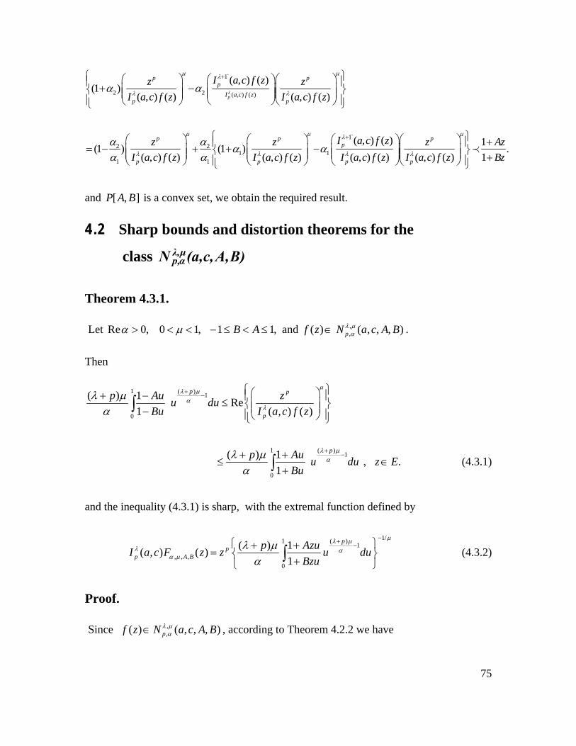
75
1̀
2 2 ( , ) ( )
1̀2 2
1 11 1
( , ) ( )(1 )
( , ) ( ) ( , ) ( )
( , ) ( )(1 ) (1 )
( , ) ( ) ( , ) ( ) ( , ) ( )
p
p pp
I a c f zp p
p pp
p p p
I a c f zz zI a c f z I a c f z
I a c f zz zI a c f z I a c f z I a c f z
λ
μ μλ
λ λ
μ μ λ
λ λ λ
α α
α α α αα α
+
+
⎧ ⎫⎛ ⎞ ⎛ ⎞⎛ ⎞⎪ ⎪+ −⎜ ⎟ ⎜ ⎟⎜ ⎟⎨ ⎬⎜ ⎟⎜ ⎟ ⎜ ⎟⎪ ⎪⎝ ⎠⎝ ⎠ ⎝ ⎠⎩ ⎭
⎛ ⎞ ⎛ ⎞ ⎛= − + + −⎜ ⎟ ⎜ ⎟ ⎜⎜ ⎟ ⎜ ⎟ ⎜
⎝ ⎠ ⎝ ⎠ ⎝
1 .( , ) ( ) 1
p
p
z AzI a c f z Bz
μ
λ
⎧ ⎫⎞⎛ ⎞ +⎪ ⎪⎟⎜ ⎟⎨ ⎬⎟⎜ ⎟ +⎪ ⎪⎠⎝ ⎠⎩ ⎭
≺
and [ , ]P A B is a convex set, we obtain the required result. 4.2 Sharp bounds and distortion theorems for the
class λ,μp,αN (a,c,A,B)
Theorem 4.3.1.
Let Re 0, 0 1, 1 1, and ( )B A f zα μ> < < − ≤ < ≤ ∈ ,, ( , , , )pN a c A Bλ μα .
Then
1 ( ) 1
0
( ) 1 Re1 ( , ) ( )
p p
p
p Au zu duBu I a c f z
μλ μ
αλ
λ μα
+− ⎧ ⎫⎛ ⎞+ − ⎪ ⎪≤ ⎜ ⎟⎨ ⎬⎜ ⎟− ⎪ ⎪⎝ ⎠⎩ ⎭
∫
1 ( ) 1
0
( ) 1 .1
pp Au u du z EBu
λ μαλ μ
α
+−+ +
≤ , ∈+∫ (4.3.1)
and the inequality (4.3.1) is sharp, with the extremal function defined by
1/1 ( ) 1
, , ,0
( ) 1( , ) ( )1
pp
p A Bp AzuI a c F z z u du
Bzu
μλ μλ α
α μλ μ
α
−+−⎧ ⎫+ +
= ⎨ ⎬+⎩ ⎭∫ (4.3.2)
Proof.
Since ,,( ) ( , , , )pf z N a c A Bλ μα∈ , according to Theorem 4.2.2 we have
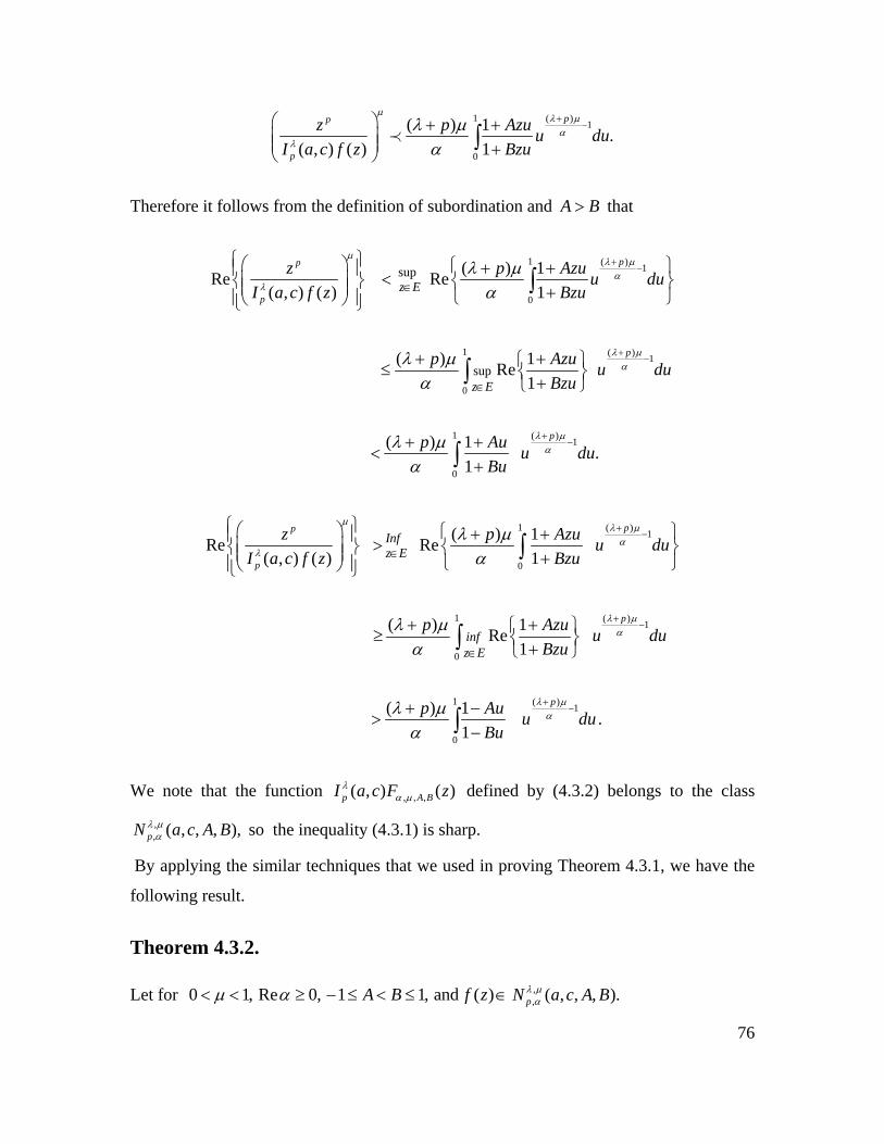
76
1 ( ) 1
0
( ) 1 .( , ) ( ) 1
pp
p
z p Azu u duI a c f z Bzu
μλ μ
αλ
λ μα
+−⎛ ⎞ + +
⎜ ⎟⎜ ⎟ +⎝ ⎠∫≺
Therefore it follows from the definition of subordination and A B> that
1 ( ) 1
0
sup ( ) 1Re Re( , ) ( ) 1
pp
pz E
z p Azu u duI a c f z Bzu
μλ μ
αλ
λ μα
+−
∈
⎧ ⎫⎛ ⎞ ⎧ ⎫+ +⎪ ⎪ < ⎜ ⎟⎨ ⎬ ⎨ ⎬⎜ ⎟ +⎩ ⎭⎪ ⎪⎝ ⎠⎩ ⎭∫
1 ( ) 1
0
sup( ) 1Re
1
p
z E
p Azu u duBzu
λ μαλ μ
α
+−
∈
+ +⎧ ⎫≤ ⎨ ⎬+⎩ ⎭∫
1 ( ) 1
0
( ) 1 .1
pp Au u duBu
λ μαλ μ
α
+−+ +
<+∫
1 ( ) 1
0
( ) 1Re Re( , ) ( ) 1
pp
p
Infz E
z p Azu u duI a c f z Bzu
μλ μ
αλ
λ μα
+−
∈
⎧ ⎫⎛ ⎞ ⎧ ⎫+ +⎪ ⎪ > ⎜ ⎟⎨ ⎬ ⎨ ⎬⎜ ⎟ +⎩ ⎭⎪ ⎪⎝ ⎠⎩ ⎭∫
1 ( ) 1
0
( ) 1Re1
p
infz E
p Azu u duBzu
λ μαλ μ
α
+−
∈
+ +⎧ ⎫≥ ⎨ ⎬+⎩ ⎭∫
1 ( ) 1
0
( ) 1 .1
pp Au u duBu
λ μαλ μ
α
+−+ −
> −∫
We note that the function , , ,( , ) ( )p A BI a c F zλ
α μ defined by (4.3.2) belongs to the class
,, ( , , , ),pN a c A Bλ μα so the inequality (4.3.1) is sharp.
By applying the similar techniques that we used in proving Theorem 4.3.1, we have the
following result.
Theorem 4.3.2.
Let for 0 1, Re 0, 1 1, and ( )A B f zμ α < < ≥ − ≤ < ≤ ∈ ,, ( , , , ).pN a c A Bλ μα
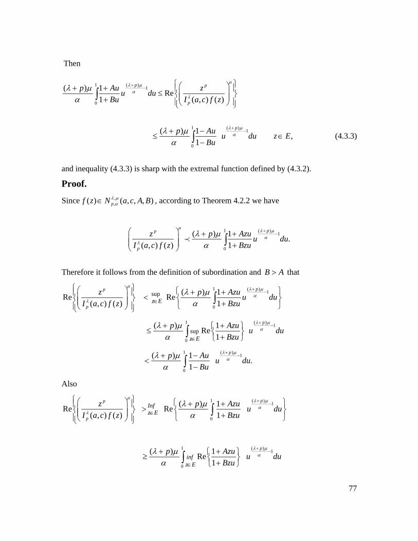
77
Then
1 ( ) 1
0
( ) 1 Re1 ( , ) ( )
p p
p
p Au zu duBu I a c f z
μλ μ
αλ
λ μα
+− ⎧ ⎫⎛ ⎞+ + ⎪ ⎪≤ ⎜ ⎟⎨ ⎬⎜ ⎟+ ⎪ ⎪⎝ ⎠⎩ ⎭
∫
1 ( ) 1
0
( ) 1 ,1
pp Au u du z EBu
λ μαλ μ
α
+−+ −
≤ ∈−∫ (4.3.3)
and inequality (4.3.3) is sharp with the extremal function defined by (4.3.2).
Proof.
Since ,,( ) ( , , , )pf z N a c A Bλ μα∈ , according to Theorem 4.2.2 we have
1 ( ) 1
0
( ) 1 .( , ) ( ) 1
pp
p
z p Azu u duI a c f z Bzu
μλ μ
αλ
λ μα
+−⎛ ⎞ + +
⎜ ⎟⎜ ⎟ +⎝ ⎠∫≺
Therefore it follows from the definition of subordination and B A> that
1 ( ) 1
0
sup ( ) 1Re Re( , ) ( ) 1
pp
pz E
z p Azu u duI a c f z Bzu
μλ μ
αλ
λ μα
+−
∈
⎧ ⎫⎛ ⎞ ⎧ ⎫+ +⎪ ⎪ < ⎜ ⎟⎨ ⎬ ⎨ ⎬⎜ ⎟ +⎩ ⎭⎪ ⎪⎝ ⎠⎩ ⎭∫
1 ( ) 1
0
sup( ) 1Re
1
p
z E
p Azu u duBzu
λ μαλ μ
α
+−
∈
+ +⎧ ⎫≤ ⎨ ⎬+⎩ ⎭∫
1 ( ) 1
0
( ) 1 .1
pp Au u duBu
λ μαλ μ
α
+−+ −
<−∫
Also
1 ( ) 1
0
( ) 1Re Re( , ) ( ) 1
pp
p
Infz E
z p Azu u duI a c f z Bzu
μλ μ
αλ
λ μα
+−
∈
⎧ ⎫⎛ ⎞ ⎧ ⎫+ +⎪ ⎪ > ⎜ ⎟⎨ ⎬ ⎨ ⎬⎜ ⎟ +⎩ ⎭⎪ ⎪⎝ ⎠⎩ ⎭∫
1 ( ) 1
0
( ) 1Re1
p
infz E
p Azu u duBzu
λ μαλ μ
α
+−
∈
+ +⎧ ⎫≥ ⎨ ⎬+⎩ ⎭∫
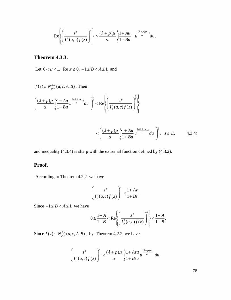
78
1 ( ) 1
0
( ) 1Re .( , ) ( ) 1
pp
p
z p Au u duI a c f z Bu
μλ μ
αλ
λ μα
+−⎧ ⎫⎛ ⎞ + +⎪ ⎪ > ⎜ ⎟⎨ ⎬⎜ ⎟ +⎪ ⎪⎝ ⎠⎩ ⎭
∫
Theorem 4.3.3.
Let 0 1, Re 0, 1 1,B Aμ α< < ≥ − ≤ < ≤ and
,,( ) ( , , , )pf z N a c A Bλ μα∈ . Then
1 ( ) 21
0
( ) 1 Re1 ( , ) ( )
p p
p
p Au zu duBu I a c f z
μλ μ
αλ
λ μα
1+ 2−
⎧ ⎫⎛ ⎞⎛ ⎞+ − ⎪ ⎪ < ⎜ ⎟⎨ ⎬⎜ ⎟ ⎜ ⎟−⎝ ⎠ ⎪ ⎪⎝ ⎠
⎩ ⎭∫
1 ( ) 1
0
( ) 1 , .1
pp Au u du z EBu
λ μαλ μ
α
1+ 2−⎛ ⎞+ +
< ∈⎜ ⎟+⎝ ⎠∫ 4.3.4)
and inequality (4.3.4) is sharp with the extremal function defined by (4.3.2).
Proof.
According to Theorem 4.2.2 we have
1 .( , ) ( ) 1
p
p
z AzI a c f z Bz
μ
λ
⎛ ⎞ +⎜ ⎟⎜ ⎟ +⎝ ⎠
≺
Since 1 1,B A− ≤ < ≤ we have
1 10 Re .1 ( , ) ( ) 1
p
p
A z AB I a c f z B
μ
λ
⎧ ⎫⎛ ⎞− +⎪ ⎪≤ < <⎜ ⎟⎨ ⎬⎜ ⎟− +⎪ ⎪⎝ ⎠⎩ ⎭
Since ,,( ) ( , , , )pf z N a c A Bλ μα∈ , by Theorem 4.2.2 we have
1 ( ) 1
0
( ) 1 .( , ) ( ) 1
pp
p
z p Azu u duI a c f z Bzu
μλ μ
αλ
λ μα
+−⎛ ⎞ + +
⎜ ⎟⎜ ⎟ +⎝ ⎠∫≺
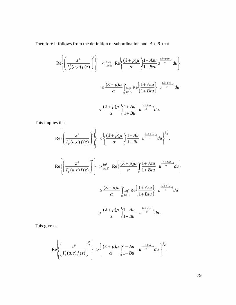
79
Therefore it follows from the definition of subordination and A B> that
1 ( ) 1
0
sup ( ) 1Re Re( , ) ( ) 1
pp
pz E
z p Azu u duI a c f z Bzu
μλ μ
αλ
λ μα
+−
∈
⎧ ⎫⎛ ⎞ ⎧ ⎫+ +⎪ ⎪ < ⎜ ⎟⎨ ⎬ ⎨ ⎬⎜ ⎟ +⎩ ⎭⎪ ⎪⎝ ⎠⎩ ⎭∫
1 ( ) 1
0
sup( ) 1Re
1
p
z E
p Azu u duBzu
λ μαλ μ
α
+−
∈
+ +⎧ ⎫≤ ⎨ ⎬+⎩ ⎭∫
1 ( ) 1
0
( ) 1 .1
pp Au u duBu
λ μαλ μ
α
+−+ +
<+∫
This implies that
2
Re( , ) ( )
p
p
zI a c f z
μ
λ
⎧ ⎫⎛ ⎞⎪ ⎪⎜ ⎟⎨ ⎬⎜ ⎟⎪ ⎪⎝ ⎠
⎩ ⎭
11 2( ) 1
0
( ) 1 .1
pp Au u duBu
λ μαλ μ
α
+−⎧ ⎫+ +
< ⎨ ⎬+⎩ ⎭∫
1 ( ) 1
0
( ) 1Re Re( , ) ( ) 1
pp
p
Infz E
z p Azu u duI a c f z Bzu
μλ μ
αλ
λ μα
+−
∈
⎧ ⎫⎛ ⎞ ⎧ ⎫+ +⎪ ⎪ > ⎜ ⎟⎨ ⎬ ⎨ ⎬⎜ ⎟ +⎩ ⎭⎪ ⎪⎝ ⎠⎩ ⎭∫
1 ( ) 1
0
( ) 1Re1
p
infz E
p Azu u duBzu
λ μαλ μ
α
+−
∈
+ +⎧ ⎫≥ ⎨ ⎬+⎩ ⎭∫
1 ( ) 1
0
( ) 1 .1
pp Au u duBu
λ μαλ μ
α
+−+ −
> −∫
This give us
2
Re( , ) ( )
p
p
zI a c f z
μ
λ
⎧ ⎫⎛ ⎞⎪ ⎪⎜ ⎟⎨ ⎬⎜ ⎟⎪ ⎪⎝ ⎠
⎩ ⎭
11 2( ) 1
0
( ) 1 .1
pp Au u duBu
λ μαλ μ
α
+−⎧ ⎫+ −
> ⎨ ⎬−⎩ ⎭∫
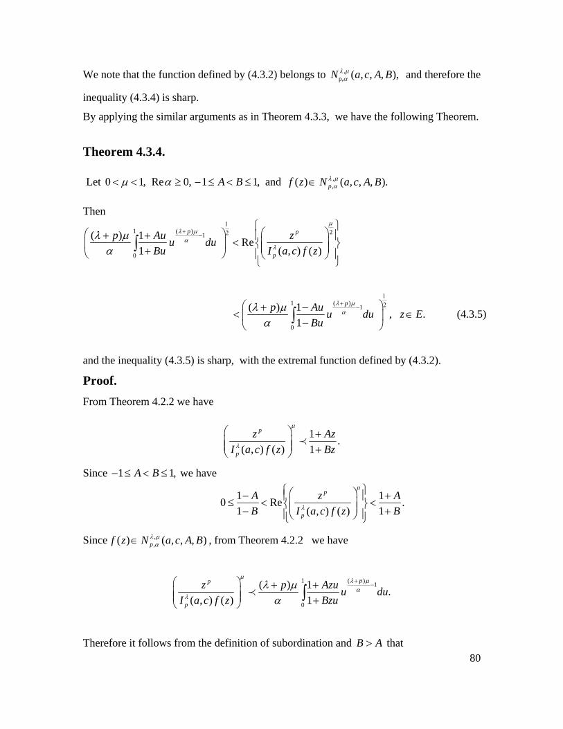
80
We note that the function defined by (4.3.2) belongs to ,p, ( , , , ),N a c A Bλ μ
α and therefore the
inequality (4.3.4) is sharp.
By applying the similar arguments as in Theorem 4.3.3, we have the following Theorem.
Theorem 4.3.4.
Let 0 1, Re 0, 1 1, and ( )A B f zμ α < < ≥ − ≤ < ≤ ∈ ,, ( , , , ).pN a c A Bλ μα
Then
1 ( ) 21
0
( ) 1 Re1 ( , ) ( )
p p
p
p Au zu duBu I a c f z
μλ μ
αλ
λ μα
1+ 2−
⎧ ⎫⎛ ⎞⎛ ⎞+ + ⎪ ⎪ < ⎜ ⎟⎨ ⎬⎜ ⎟ ⎜ ⎟+⎝ ⎠ ⎪ ⎪⎝ ⎠
⎩ ⎭∫
1 ( ) 1
0
( ) 1 , .1
pp Au u du z EBu
λ μαλ μ
α
1+ 2−⎛ ⎞+ −
< ∈⎜ ⎟−⎝ ⎠∫ (4.3.5)
and the inequality (4.3.5) is sharp, with the extremal function defined by (4.3.2).
Proof. From Theorem 4.2.2 we have
1 .( , ) ( ) 1
p
p
z AzI a c f z Bz
μ
λ
⎛ ⎞ +⎜ ⎟⎜ ⎟ +⎝ ⎠
≺
Since 1 1,A B− ≤ < ≤ we have
1 10 Re .1 ( , ) ( ) 1
p
p
A z AB I a c f z B
μ
λ
⎧ ⎫⎛ ⎞− +⎪ ⎪≤ < <⎜ ⎟⎨ ⎬⎜ ⎟− +⎪ ⎪⎝ ⎠⎩ ⎭
Since ,,( ) ( , , , )pf z N a c A Bλ μα∈ , from Theorem 4.2.2 we have
1 ( ) 1
0
( ) 1 .( , ) ( ) 1
pp
p
z p Azu u duI a c f z Bzu
μλ μ
αλ
λ μα
+−⎛ ⎞ + +
⎜ ⎟⎜ ⎟ +⎝ ⎠∫≺
Therefore it follows from the definition of subordination and B A> that
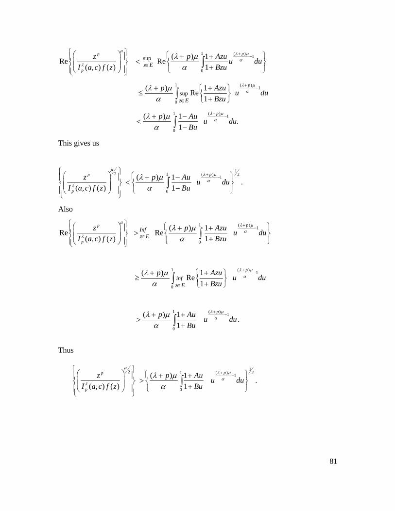
81
1 ( ) 1
0
sup ( ) 1Re Re( , ) ( ) 1
pp
pz E
z p Azu u duI a c f z Bzu
μλ μ
αλ
λ μα
+−
∈
⎧ ⎫⎛ ⎞ ⎧ ⎫+ +⎪ ⎪ < ⎜ ⎟⎨ ⎬ ⎨ ⎬⎜ ⎟ +⎩ ⎭⎪ ⎪⎝ ⎠⎩ ⎭∫
1 ( ) 1
0
sup( ) 1Re
1
p
z E
p Azu u duBzu
λ μαλ μ
α
+−
∈
+ +⎧ ⎫≤ ⎨ ⎬+⎩ ⎭∫
1 ( ) 1
0
( ) 1 .1
pp Au u duBu
λ μαλ μ
α
+−+ −
<−∫
This gives us
2
( , ) ( )
p
p
zI a c f z
μ
λ
⎧ ⎫⎛ ⎞⎪ ⎪⎜ ⎟⎨ ⎬⎜ ⎟⎪ ⎪⎝ ⎠⎩ ⎭
11 2( ) 1
0
( ) 1 .1
pp Au u duBu
λ μαλ μ
α
+−⎧ ⎫+ −
< ⎨ ⎬−⎩ ⎭∫
Also
1 ( ) 1
0
( ) 1Re Re( , ) ( ) 1
pp
p
Infz E
z p Azu u duI a c f z Bzu
μλ μ
αλ
λ μα
+−
∈
⎧ ⎫⎛ ⎞ ⎧ ⎫+ +⎪ ⎪ > ⎜ ⎟⎨ ⎬ ⎨ ⎬⎜ ⎟ +⎩ ⎭⎪ ⎪⎝ ⎠⎩ ⎭∫
1 ( ) 1
0
( ) 1Re1
p
infz E
p Azu u duBzu
λ μαλ μ
α
+−
∈
+ +⎧ ⎫≥ ⎨ ⎬+⎩ ⎭∫
1 ( ) 1
0
( ) 1 .1
pp Au u duBu
λ μαλ μ
α
+−+ +
> +∫
Thus
2
( , ) ( )
p
p
zI a c f z
μ
λ
⎧ ⎫⎛ ⎞⎪ ⎪⎜ ⎟⎨ ⎬⎜ ⎟⎪ ⎪⎝ ⎠⎩ ⎭
11 2( ) 1
0
( ) 1 .1
pp Au u duBu
λ μαλ μ
α
+−⎧ ⎫+ +
> ⎨ ⎬+⎩ ⎭∫
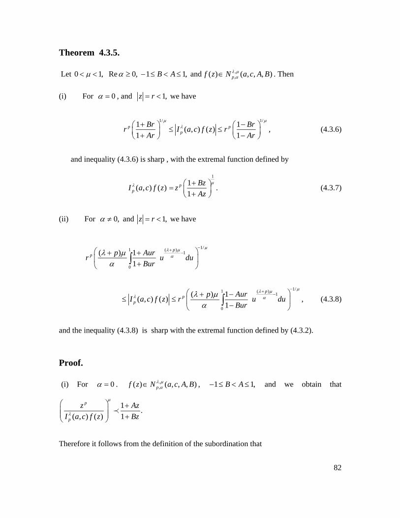
82
Theorem 4.3.5.
Let 0 1, Re 0, 1 1,B Aμ α< < ≥ − ≤ < ≤ and ,,( ) ( , , , )pf z N a c A Bλ μα∈ . Then
(i) For 0α = , and 1,z r= < we have
1/ 1/1 1( , ) ( ) ,
1 1p p
pBr Brr I a c f z rAr Ar
μ μλ+ −⎛ ⎞ ⎛ ⎞≤ ≤⎜ ⎟ ⎜ ⎟+ −⎝ ⎠ ⎝ ⎠
(4.3.6)
and inequality (4.3.6) is sharp , with the extremal function defined by
1
1( , ) ( ) .1
pp
BzI a c f z zAz
μλ +⎛ ⎞= ⎜ ⎟+⎝ ⎠ (4.3.7)
(ii) For 0,α ≠ and 1,z r= < we have
1/1 ( ) 1
0
( ) 11
pp p Aurr u du
Bur
μλ μαλ μ
α
−+−⎛ ⎞+ +
⎜ ⎟+⎝ ⎠∫
1/1 ( ) 1
0
( ) 1( , ) ( ) ,1
pp
pp AurI a c f z r u du
Bur
μλ μλ αλ μ
α
−+−⎛ ⎞+ −
≤ ≤ ⎜ ⎟−⎝ ⎠∫ (4.3.8)
and the inequality (4.3.8) is sharp with the extremal function defined by (4.3.2).
Proof.
(i) For 0α = . ,,( ) ( , , , )pf z N a c A Bλ μα∈ , 1 1,B A− ≤ < ≤ and we obtain that
1 .( , ) ( ) 1
p
p
z AzI a c f z Bz
μ
λ
⎛ ⎞ +⎜ ⎟⎜ ⎟ +⎝ ⎠
≺
Therefore it follows from the definition of the subordination that
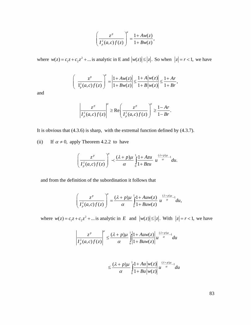
83
1 ( ) ,( , ) ( ) 1 ( )
p
p
z Aw zI a c f z Bw z
μ
λ
⎛ ⎞ +=⎜ ⎟⎜ ⎟ +⎝ ⎠
where 2
1 2( ) ...w z c z c z= + + is analytic in E and ( ) .w z z≤ So when 1,z r= < we have
p
p
1 ( )z 1 ( ) 1 ,I ( , ) ( ) 1 ( ) 1 ( ) 1
A w zAw z Ara c f z Bw z B w z Br
μ
λ
⎛ ⎞ ++ += ≤ ≤⎜ ⎟⎜ ⎟ + + +⎝ ⎠
and
1Re .( , ) ( ) ( , ) ( ) 1
p p
p p
z z ArI a c f z I a c f z Br
μ μ
λ λ
⎛ ⎞ −≥ ≥⎜ ⎟⎜ ⎟ −⎝ ⎠
It is obvious that (4.3.6) is sharp, with the extremal function defined by (4.3.7). (ii) If 0,α ≠ apply Theorem 4.2.2 to have
1 ( ) 1
0
( ) 1 .( , ) ( ) 1
pp
p
z p Azu u duI a c f z Bzu
μλ μ
αλ
λ μα
+−⎛ ⎞ + +
⎜ ⎟⎜ ⎟ + ⎝ ⎠∫≺
and from the definition of the subordination it follows that
1 ( ) 1
0
( ) 1 ( ) ,( , ) ( ) 1 ( )
pp
p
z p Auw z u duI a c f z Buw z
μλ μ
αλ
λ μα
+−⎛ ⎞ + +
= ⎜ ⎟⎜ ⎟ +⎝ ⎠∫
where 2
1 2( ) ...w z c z c z= + + is analytic in E and ( ) .w z z≤ With 1,z r= < we have
1 ( ) 1
0
( ) 1 ( )( , ) ( ) 1 ( )
pp
p
z p Auw z u duI a c f z Buw z
μλ μ
αλ
λ μα
+−+ +
≤ +∫
1 ( ) 1
0
1 ( )( )1 ( )
pAu w zp u duBu w z
λ μαλ μ
α
+−++
≤ +∫
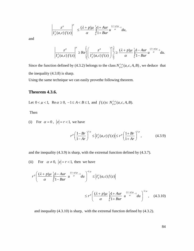
84
( , ) ( )
p
p
zI a c f z
μ
λ 1 ( ) 1
0
( ) 1 ,1
pp Aur u duBur
λ μαλ μ
α
+−+ +
≤ +∫
and
Re( , ) ( ) ( , ) ( )
p p
p p
z zI a c f z I a c f z
μ μ
λ λ
⎧ ⎫⎛ ⎞⎪ ⎪≥ ≥⎜ ⎟⎨ ⎬⎜ ⎟⎪ ⎪⎝ ⎠⎩ ⎭
1 ( ) 1
0
( ) 1 .1
pp Aur u duBur
λ μαλ μ
α
+−+ −
−∫
Since the function defined by (4.3.2) belongs to the class ,, ( , , , )pN a c A Bλ μα , we deduce that
the inequality (4.3.8) is sharp.
Using the same technique we can easily provethe following theorem.
Theorem 4.3.6.
Let 0 1, Re 0, 1 1,A Bμ α< < ≥ − ≤ < ≤ and ,,( ) ( , , , ).pf z N a c A Bλ μα∈
Then (i) For 0α = , 1,z r= < we have
1/ 1/1 1( , ) ( ) ,1 1
p pp
Br Brr I a c f z rAr Ar
μ μλ− +⎛ ⎞ ⎛ ⎞≤ ≤⎜ ⎟ ⎜ ⎟− +⎝ ⎠ ⎝ ⎠
(4.3.9)
and the inequality (4.3.9) is sharp, with the extremal function defined by (4.3.7).
(ii) For 0,α ≠ 1,z r= < then we have
1/1 ( ) 1
0
( ) 1 ( , ) ( )1
pp
pp Aurr u du I a c f z
Bur
μλ μλαλ μ
α
−+ −⎛ ⎞+ −
≤⎜ ⎟−⎝ ⎠∫
1/1 ( ) 1
0
( ) 1 ,1
pp p Aurr u du
Bur
μλ μαλ μ
α
−+ −⎛ ⎞+ +
≤ ⎜ ⎟+⎝ ⎠∫ (4.3.10)
and inequality (4.3.10) is sharp, with the extremal function defined by (4.3.2).
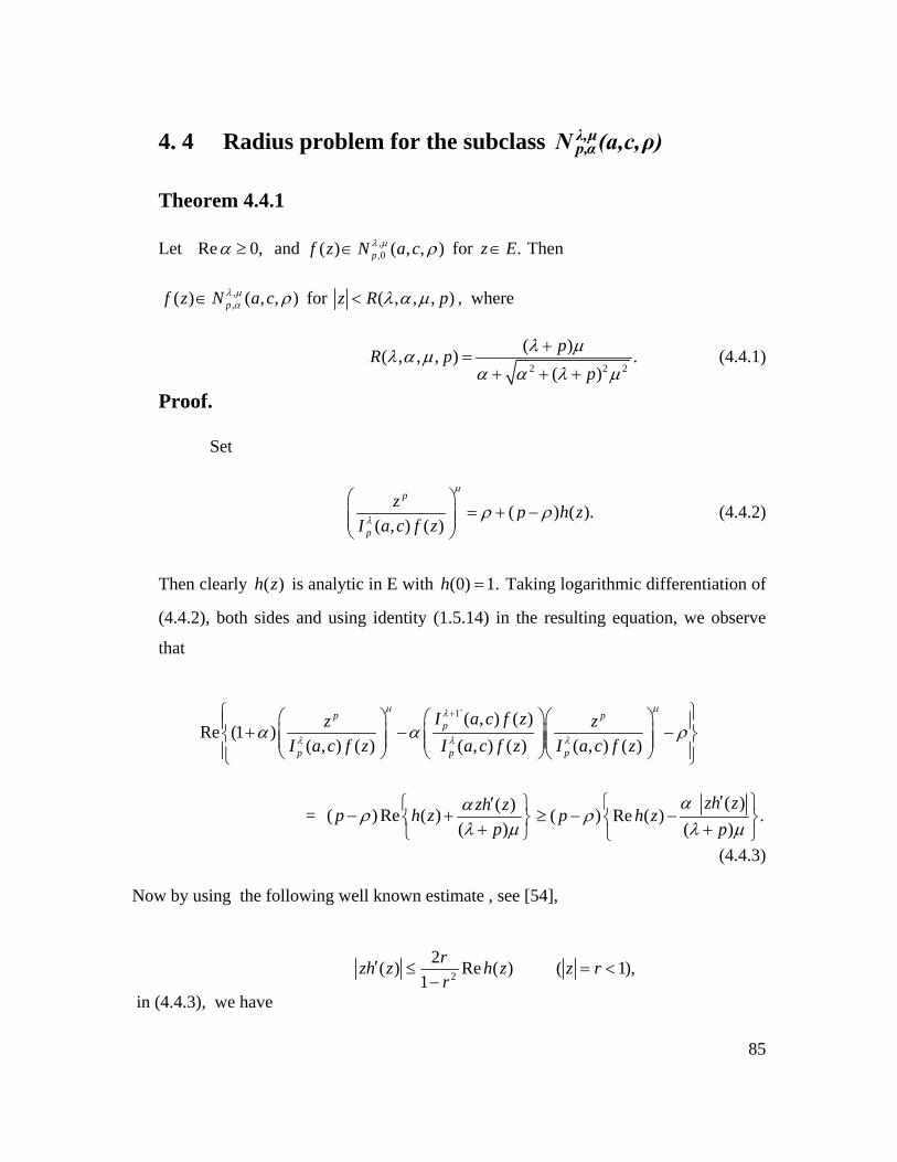
85
4. 4 Radius problem for the subclass λ,μ
p,αN (a,c,ρ) Theorem 4.4.1
Let Re 0,α ≥ and ,,0( ) ( , , )pf z N a cλ μ ρ∈ for .z E∈ Then
,,( ) ( , , )pf z N a cλ μα ρ∈ for ( , , , )z R pλ α μ< , where
2 2 2
( )( , , , ) .( )pR p
pλ μλ α μ
α α λ μ+
=+ + +
(4.4.1)
Proof.
Set
( ) ( ).( , ) ( )
p
p
z p h zI a c f z
μ
λ ρ ρ⎛ ⎞
= + −⎜ ⎟⎜ ⎟⎝ ⎠
(4.4.2)
Then clearly ( )h z is analytic in E with (0) 1.h = Taking logarithmic differentiation of
(4.4.2), both sides and using identity (1.5.14) in the resulting equation, we observe
that
1`( , ) ( )Re (1 )
( , ) ( ) ( , ) ( ) ( , ) ( )
p pp
p p p
I a c f zz zI a c f z I a c f z I a c f z
μ μλ
λ λ λα α ρ+⎧ ⎫⎛ ⎞ ⎛ ⎞⎛ ⎞⎪ ⎪+ − −⎜ ⎟ ⎜ ⎟⎜ ⎟⎨ ⎬⎜ ⎟ ⎜ ⎟⎜ ⎟⎪ ⎪⎝ ⎠ ⎝ ⎠⎝ ⎠⎩ ⎭
= ( )( ) Re ( )( )
zh zp h zp
αρλ μ
′⎧ ⎫− +⎨ ⎬+⎩ ⎭
( )( ) Re ( ) .
( )zh z
p h zp
αρ
λ μ′⎧ ⎫
≥ − −⎨ ⎬+⎩ ⎭
(4.4.3) Now by using the following well known estimate , see [54],
2
2( ) Re ( ) ( 1),1
rzh z h z z rr
′ ≤ = <−
in (4.4.3), we have
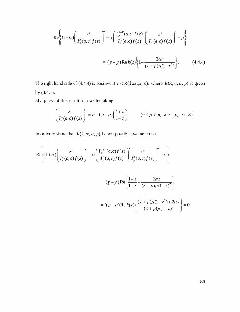
86
1`( , ) ( )Re (1 )
( , ) ( ) ( , ) ( ) ( , ) ( )
p pp
p p p
I a c f zz zI a c f z I a c f z I a c f z
μ μλ
λ λ λα α ρ+⎧ ⎫⎛ ⎞ ⎛ ⎞⎛ ⎞⎪ ⎪+ − −⎜ ⎟ ⎜ ⎟⎜ ⎟⎨ ⎬⎜ ⎟ ⎜ ⎟⎜ ⎟⎪ ⎪⎝ ⎠ ⎝ ⎠⎝ ⎠⎩ ⎭
= 2
2( ) Re ( ) 1 .( ) (1 )
rp h zp r
αρλ μ
⎧ ⎫− −⎨ ⎬+ −⎩ ⎭
(4.4.4)
The right hand side of (4.4.4) is positive if ( , , , ),r R pλ α μ< where ( , , , )R pλ α μ is given
by (4.4.1).
Sharpness of this result follows by taking
1( ) (0 , , )( , ) ( ) 1
p
p
z zp p p z EI a c f z z
μ
λ ρ ρ ρ λ⎛ ⎞ +⎛ ⎞= + − . ≤ < > − ∈⎜ ⎟ ⎜ ⎟⎜ ⎟ −⎝ ⎠⎝ ⎠
.
In order to show that ( , , , )R pλ α μ is best possible, we note that
1`( , ) ( )
Re (1 )( , ) ( ) ( , ) ( ) ( , ) ( )
p pp
p p p
I a c f zz zI a c f z I a c f z I a c f z
μ μλ
λ λ λα α ρ+⎧ ⎫⎛ ⎞ ⎛ ⎞⎛ ⎞⎪ ⎪+ − −⎜ ⎟ ⎜ ⎟⎜ ⎟⎨ ⎬⎜ ⎟ ⎜ ⎟⎜ ⎟⎪ ⎪⎝ ⎠ ⎝ ⎠⎝ ⎠⎩ ⎭
2
1 2( ) Re1 ( ) (1 )
z zpz p z
αρλ μ
⎧ ⎫+= − +⎨ ⎬− + −⎩ ⎭
2
2
( ) (1 ) 2(( ) Re ( ) 0.( ) (1 )
p z zp h zp z
λ μ αρλ μ
⎧ ⎫+ − += − =⎨ ⎬+ −⎩ ⎭
87
CHAPTER 5
SOME NEW CLASSES OF MEROMORPHIC
AND ANALYTIC FUNCTIONS
5.1 Introduction
In this chapter we shall be concerned mainly with problems of p-valent and
meromorphic functions. Making use of the generalized hypergeometric functions, we
introduce certain new subclass 1( , , , , , )kT p q sλ α ρ of analytic functions defined by
Dziok-Srivastava operator in the unit disc. Many interesting subclasses of analytic
functions, associated with the Dziok-Srivastava operator , , 1( )p q sH α and its many special
cases, were investigated recently by Dziok and Srivastava [22,23], Gangadharan et al
[26], Liu [46], Liu and Srivastava [48], we refer also to [46,80,106].
The main object is to investigate the various properties and characteristics of analytic
functions belonging to the subclass 1( , , , , , )kT p q sλ α ρ . Apart from this, we obtain a
number of new applications for this class of p-valent functions. In section 5.2, we define
the class 1( , , , , , )kT p q sλ α ρ and investigate a number of inclusion relationships. We
derive a sharp radius for the class 1( , , , , , )kT p q sλ α ρ . We also study interesting results on
the Hadamard products of functions belonging to the p-valently function class
1( , , , , , )kT p q sλ α ρ and some other interesting properties of p-valent functions which are
defined here by means of a certain linear integral operator , , 1( ).p q sH α
In this chapter, we also investigate the various important properties and characteristics of
the classes ( , , , , )kMB q sα λ ρ and ( , , , , )kMT q sα λ ρ of meromorphic functions.
In section 5.3, we introduce and study two new subclasses, ( , , , , )kMB q sα λ ρ and
( , , , , )kMT q sα λ ρ of meromorphic functions defined by using a meromorphic analogue
of the Choi−Saigo−Srivastava operator for the generalized hypergeometric function in
the punctured unit disk .E∗ We note that the operator , , 1( )q sHλ α is closely related to the
88
Choi−Saigo−Srivastava operator [17] for analytic functions, which includes the integral
operator studied by Liu [47] and Noor et al [70,74]. Meromorphically functions have
been extensively studied by several authors Mogra [61,62], Uralegaddi and Ganigi [116],
Uralegaddi and Somanatha [117], Aouf [3,4], Srivastava et al [109], Owa et al [81],
Joshi and Aouf [32], Joshi and Srivastava [33], Aouf et al [5], Raina and Srivastava [93]
and Yang [122].
We derive several inclusion relationships for these function classes ( , , , , )kMB q sα λ ρ
and ( , , , , ).kMT q sα λ ρ In section 5.4, we prove sharp radius theorem and integral
preserving property for the class ( , , , , ).kMB q sα λ ρ In the final section 5.5, we are mainly
concerned with convolution preserving properties of the function classes
( , , , , )kMB q sα λ ρ and ( , , , , ).kMT q sα λ ρ All the results here are new.
5.2 The class k 1T (λ,α , p,q,s,ρ) Definition 5.2.1.
Let ( ).f p∈A Then 1( , , , , , ),kf T p q sλ α ρ∈ if and only if
, , 1 , , 1( ) ( ) ( 1) ( )(1 ) ( ), ,p q s p q s
kp p
H f z H f zP z E
z zα α
λ λ ρ+⎧ ⎫
− + ∈ ∈⎨ ⎬⎩ ⎭
where 0, 2kλ > ≥ and 0 .pρ≤ <
5. 2. 1 Inclusion results for the class k 1T (λ,α , p,q,s,ρ) Theorem 5.2.1.
Let 1Re 0α > . Then 1 1 1( , , , , , ) (0, , , , , ),k kT p q s T p q sλ α ρ α ρ⊂
where 1ρ is given by
1 1(1 )(2 1),ρ ρ ρ γ= + − − (5.2.1)
and
89
1
11 Re
10
1 .t dtλαγ
−⎛ ⎞⎜ ⎟⎝ ⎠
⎛ ⎞⎜ ⎟= +⎜ ⎟⎝ ⎠∫
Proof.
Let 1( , , , , , )kf T p q sλ α ρ∈ and set
, , 1
1 2
( ) ( ) 1 1( ) ( ) ( ) ( ) ( ).4 2 4 2
p q sp
H f z k kh z h z h zzα
= = + − − (5.2.2)
Then ( )h z is analytic in E with (0) 1.h = Taking logarithmic differentiation of (5.2.2)
both sides and using the identity (1.5.19) in the resulting equation, we deduce that
, , 1
, , 1
( ( ) ( )) ( ) .( ) ( ) ( )
p q s
p q s
z H f z zh zpH f z h z
αα
′ ′= +
Using identity (1.5.19) in the above equation, we have
1 , , 1 1 , , 1
, , 1
( 1) ( ) ( ) ( ) ( ) ( ) .( ) ( ) ( )
p q s p q s
p q s
H f z p H f z zh zpH f z h z
α α α αα
+ − − ′= +
From the above equation we can easily deduce that
, , 1 , , 1
1
( ) ( ) ( 1) ( ) ( )(1 ) ( ) ( )p q s p q skp p
H f z H f z zh zh z Pz zα α λλ λ ρ
α+ ⎧ ⎫⎧ ⎫ ′
− + = + ∈⎨ ⎬ ⎨ ⎬⎩ ⎭ ⎩ ⎭
for .z E∈
Using Lemma 1.6.4, we see that 1( ),kh P ρ∈ z E∈ where 1ρ is given by (5.2.1). and the
proof is complete.
Theorem 5.2.2.
1 1 2 1( , , , , , ) ( , , , , , )k kT p q s T p q sλ α ρ λ α ρ⊂ for 2 10 .λ λ≤ <
90
Proof.
For 2 0,λ = the proof is immediate. Let 2 0λ > and let 1( , , , , , ).kf T p q sλ α ρ∈ Then there
exist two functions 1 2, ( )kH H P ρ∈ such that, from Definition 5.2.1 and Theorem 5.2.1,
, , 1 , , 11 1 1
( ) ( ) ( 1) ( )(1 ) ( ),p q s p q s
p p
H f z H f zH z
z zα α
λ λ+
− + =
and
, , 12
( )( ).p q s
p
HH z
zα
=
Hence
, , 1 , , 1 2 22 2 1 2
1 1
( ) ( ) ( 1) ( )(1 ) ( ) (1 ) ( ).p q s p q s
p p
H f z H f zH z H z
z zα α λ λλ λ
λ λ+
− + = + − (5.2.3)
Since the class ( )kP ρ is a convex set, see [72], it follows that the right hand side of
(5.2.3) belongs to ( )kP ρ and this proves the result.
5. 2. 2 Radius problem for the class k 1T (λ,α , p,q,s,ρ) Theorem 5.2.3
Let 1(0, , , , , )kf T p q sα ρ∈ for .z E∈ Then 1( , , , , , )kf T p q sλ α ρ∈ for 1( , ),z R α λ<
where
11 1 22
1
( , )Rα
α λλ λ α
=+ +
. (5.2.4)
Proof.
Set
, , 1( ) ( )( ) ( ) , .p q s
kp
H f zp h z h P
zα
ρ ρ= − + ∈
Now proceeding as in Theorem 5.2.1, we have
91
, , 1 , , 1( ) ( ) ( 1) ( )(1 ) p q s p q s
p p
H f z H f zz zα α
λ λ ρ+⎧ ⎫
− + −⎨ ⎬⎩ ⎭
1
( )( ) ( ) zh zp h z λρα
⎧ ⎫′= − +⎨ ⎬
⎩ ⎭
1 21 2
1 1
( ) ( )1 1( ) ( ) ( ) ( ) ( ) ,4 2 4 2
zh z zh zk kp h z h zλ λρα α
⎡ ⎤⎧ ⎫ ⎧ ⎫′ ′= − + + − − +⎨ ⎬ ⎨ ⎬⎢ ⎥
⎩ ⎭ ⎩ ⎭⎣ ⎦ (5.2.5)
where we have used (1.3.8) and 1 2, , .h h P z E∈ ∈ Using the following well known
estimates, see [54]
2
2( ) Re{ ( )}, ( 1), 1, 2,1i i
rzh z h z z r ir
′ ≤ = < =−
we have
1 1
Re ( ) ( ) Re ( ) ( )i i i ih z zh z h z zh zλ λα α
⎧ ⎫⎧ ⎫ ⎪ ⎪′ ′+ ≥ −⎨ ⎬ ⎨ ⎬⎪ ⎪⎩ ⎭ ⎩ ⎭
21
2Re ( ) 1 .(1 )i
rh zr
λα
⎧ ⎫⎪ ⎪≥ −⎨ ⎬−⎪ ⎪⎩ ⎭
The right hand side of this inequality is positive if 1 1( , ),r R α λ< where 1( , )R α λ is given
by (5.2.4). Consequently it follows from (5.2.5) that ( , , , , , )kf T p q sλ α ρ∈ for
1 1( , ).z R α λ<
Sharpness of this result follows by taking 1( )1i
zh zz
+=
− in (5.2.5), 1, 2.i =
5. 2. 3 The class k 1T (λ,α , p,q,s,ρ) under convolution operator
Theorem 5.2.4.
Let 1( , , , , , ),kf T p q sλ α ρ∈ and let ( ),C pφ ∈ where ( )C p is the class of p-valent convex
functions . Then 1( , , , , , ).kf T p q sφ λ α ρ∗ ∈
92
Proof.
Let .F fφ= ∗ Then, we have
, , 1 , , 1( ) ( ) ( 1) ( ) ( )(1 ) ( ),p q s p q sp p p
H F z H F z z G zz z zα α φλ λ
+⎧ ⎫− + = ∗⎨ ⎬
⎩ ⎭
where , , 1 , , 1( ) ( ) ( 1) ( )
( ) (1 ) ( ).p q s p q skp p
H f z H f zG z P
z zα α
λ λ ρ+⎧ ⎫
= − + ∈⎨ ⎬⎩ ⎭
Therefore, we have
1 2 1, 2( ) 1 ( ) 1 ( )( ) ( ) ( ) ( ) ( ) ( ) ( ) , .
4 2 4 2p p p
z k z k zG z p g z p g z g g Pz z zφ φ φρ ρ ρ ρ⎧ ⎫ ⎧ ⎫⎛ ⎞ ⎛ ⎞∗ = + − ∗ + − − − ∗ + ∈⎨ ⎬ ⎨ ⎬⎜ ⎟ ⎜ ⎟
⎝ ⎠ ⎝ ⎠⎩ ⎭ ⎩ ⎭
Since ( ),C pφ ∈ ( ) 1Re , ,2p
z z Ezφ⎧ ⎫ > ∈⎨ ⎬⎩ ⎭
and so using Lemma 1.6.5, we conclude that
1( , , , , , ).kF f T p q sφ λ α ρ= ∗ ∈
5. 2. 4 Behavior of the p-valently integral operator in the
class k 1T (λ,α , p,q,s,ρ)
Theorem 5. 2. 5.
For a function ( ) ( )f z p∈A and ,pδ > − the integral operator , : ( ) ( )p p pδ →A AF
as defined by (1.5.5).
If
, , 1 , , 1( ) ( )( ) ( ) ( )(1 ) ( ),p q s p q s
kp p
H f z H f zP
z zδα α
λ λ ρ⎧ ⎫
− + ∈⎨ ⎬⎩ ⎭
,pF (5.2.6)
93
then
, , 12
( ) ( )( )( ),p q s
kp
H f zP
zδα
ρ∈,pF
where 2ρ is given by
2 2(1 )(2 1),ρ ρ ρ γ= + − − (5.2.7)
and
1
1 Re( )
20
1 .pt dtλ
δγ−
+⎛ ⎞
= +⎜ ⎟⎜ ⎟⎝ ⎠∫
Proof.
Let
, , 11 2
( ) ( )( ) 1̀ 1̀( ) ( ) ( ) ( ) ( ),4 2 4 2
p q sp
H f z k kh z h z h zz
δα= = + − −,pF
(5.2.8 )
then the hypothesis (5.2.6) in conjection with (1.5.6 ) would yield
, , 1 , , 1( ) ( )( ) ( ) ( ) ( )(1 ) ( ) ( )p q s p q s
kp p
H f z H f z zh zh z Pz z p
δα α λλ λ ρδ
⎧ ⎫ ′⎧ ⎫− + = + ∈⎨ ⎬ ⎨ ⎬+⎩ ⎭⎩ ⎭
,pF for .z E∈
Consequently
( )( ) ( ), 1, 2, 0 ,ii
zh zh z P i pp
λ ρ ρδ
′⎧ ⎫+ ∈ = ≤ <⎨ ⎬+⎩ ⎭
and .z E∈
Using Lemma 1.6.4, with 1 ,( )p
λλδ
=+
we have { } 2Re ( ) ,ih z ρ> where 2ρ is given by
(5.2.7), and the proof is complete.
5.3 On certain subclasses of meromorphic functions
Next by using the operator , , 1( ),q sHλ α we introduce some new classes of meromorphic
functions.
94
Definition 5. 3. 1.
Let .f M∈ Then ( , , , , ),kf MB q sα λ ρ∈ if and only if
2 2, , 1 1, , 1(1 ) ( ( ) ( )) ( ( ) ( )) ( ), ,q s q s kz H f z z H f z P z Eλ λα α α α ρ+′ ′− − − ∈ ∈
where 0, 2 and 0 1.kα ρ> ≥ ≤ < Definition 5. 3. 2.
Let .f M∈ Then ( , , , , ),kf MT q sα λ ρ∈ if and only if
, , 1 1, , 1(1 ) ( ( ) ( )) ( ( ) ( )) ( ), ,q s q s kz H f z z H f z P z Eλ λα α α α ρ+− + ∈ ∈
where 0, 2 and 0 1.kα ρ> ≥ ≤ <
5. 3. 1 Some inclusion results for the some subclasses of meromorphic
functions
Theorem 5. 3. 3.
Let ( , , , , )kf MB q sα λ ρ∈ . Then
2, , 1 3( ( ) ( )) ( ),q s kz H f z Pλ α ρ′− ∈
where 3ρ is given by
3 3(1 )(2 1),ρ ρ ρ γ= + − − (5.3.1) and
11 Re
30
1 .t dtαλγ
−⎛ ⎞⎜ ⎟⎝ ⎠
⎛ ⎞= +⎜ ⎟⎜ ⎟
⎝ ⎠∫
95
Proof.
Let 2
, , 1 1 21 1( ( ) ( )) ( ) ( ) ( ) ( ) ( ).
4 2 4 2q sk kz H f z p z p z p zλ α ′− = = + − − (5.3.2)
Then ( )p z is analytic in E with (0) 1.p = From the above equation (5.3.2) we can write
, , 1{ ( ( ) ( ))} ( ).q sz z H f z h zλ α ′− = (5.3.3)
Using identity (1.5.25) in the equation (5.3.3), we have
{ }1, , 1 , , 1( ) ( ) ( 1) ( ) ( ) ( ).q s q sz H f z H f z h zλ λλ α λ α+− − + = (5.3.4)
Some simple computations yields
2 2
, , 1 1, , 1(1 ) ( ( ) ( )) ( ( ) ( )) ( ) ( ) .q s q sz H f z z H f z p z zp zλ λαα α α αλ+
⎧ ⎫′ ′ ′− − − = +⎨ ⎬⎩ ⎭
Since ( , , , , )kf MB q sα λ ρ∈ , so ( ) ( ) ( ) for .kp z zp z P z Eα ρλ
⎧ ⎫′+ ∈ ∈⎨ ⎬⎩ ⎭
Using Lemma 1.6.4, we see that 3( ),kp P ρ∈ where 3ρ is given by (5.3.1) and the proof
is complete.
Theorem 5. 3. 4.
For 2 10 ,α α≤ < 1 2( , , , , ) ( , , , , ).k kMT q s MT q sα λ ρ α λ ρ⊂ Proof.
For 2 0,α = the proof is immediate. Let 2 0α > and let 1( , , , , ).kf MT q sα λ ρ∈ Then
2 , , 1 2 1, , 1(1 ) ( ( ) ( )) ( ( ) ( ))q s q sz H f z z H f zλ λα α α α+− +
96
( ) ( ) ( )2 1, , 1 1 , , 1 1 1, , 1
1 2
( 1) ( ) ( ) (1 ) ( ) ( ) ( ) ( )q s q s q sz H f z H f z H f zλ λ λα α α α α α αα α +
⎡ ⎤= − + − +⎢ ⎥
⎣ ⎦
2 21 2 1 2
1 1
(1 ) ( ) ( ), , ( )kH z H z H H Pα α ρα α
= − + ∈
Since ( )kP ρ is a convex set, see [72], we conclude that 2( , , , , ) for .kf MT q s z Eα λ ρ∈ ∈
Now by using Theorem 5.3.3 and the lines of proof of Theorem 5.3.4 we can easily prove
the following result.
Theorem 5.3.5.
For 2 10 ,α α≤ < 1 2( , , , , ) ( , , , , ).k kMB q s MB q sα λ ρ α λ ρ⊂ 5. 4 Radius problem and an integral preserving property for
a subclass of meromorphic functions
Theorem 5. 4. 1.
Let (0, , , , )kf MB q sλ ρ∈ for .z E∈ Then ( , , , , )kf MB q sα λ ρ∈ for ( , )z R α λ< , where
2 2 2( , ) .R λα λ
α α λ=
+ + (5.4.1)
Proof.
Set
2, , 1( ( ) ( )) (1 ) ( ) , .q s kz H f z h z h Pλ α ρ ρ′− = − + ∈
Now proceeding as in Theorem 5.3.3, we have
2 2, , 1 1, , 1(1 ) ( ( ) ( )) ( ( ) ( ))q s q sz H f z z H f zλ λα α α α ρ+′ ′− − − − (1 ) ( ) ( )h z zh zαρ
λ⎧ ⎫′= − +⎨ ⎬⎩ ⎭
= 1 1 2 21 1(1 ) ( ) ( ) ( ) ( ) ( ) ( ) ,
4 2 4 2k kh z zh z h z zh zα αρ
λ λ⎡ ⎤⎧ ⎫ ⎧ ⎫′ ′− + + − − +⎨ ⎬ ⎨ ⎬⎢ ⎥⎩ ⎭ ⎩ ⎭⎣ ⎦
( 5.4.2)
97
where we have used (1.3.8) and 1 2, , .h h P z E∈ ∈ Using the following well known
estimate [54]
2
2( ) Re{ ( )}, ( 1), 1, 2,1i i
rzh z h z z r ir
′ ≤ = < =−
we have
Re ( ) ( ) Re ( ) ( )i i i ih z zh z h z zh zα αλ λ
⎧ ⎫ ⎧ ⎫′ ′+ ≥ −⎨ ⎬ ⎨ ⎬⎩ ⎭ ⎩ ⎭
2
2Re ( ) 1 .(1 )i
rh zr
αλ
⎧ ⎫≥ −⎨ ⎬−⎩ ⎭
The right hand side of this inequality is positive if ( , ),r R α λ< where 2 ( , )R α λ is given
by (5.4.1). Consequently it follows from (5.4.2) that ( , , , , )kf MB q sα λ ρ∈
for 2 ( , )z R α λ< . Sharpness of this result follows by taking 1( )1i
zh zz
+=
− in (5.4.2),
1, 2.i =
Theorem 5.4.2.
Let (0, , , , )kf MB q sλ ρ∈ and let
10
( )( ) ( ) ( 0, ).z
f z t f t dt z Ez
δδ δ
δ δ ∗+= > ∈∫F (5.4.3)
Then
2, , 1 4( ( ) ( )( )) ( ),q s kz H f z Pλ δα ρ′− ∈F
where 4ρ is given by
4 4(1 )(2 1),ρ ρ ρ γ= + − − (5.4.4)
and 111 Re
40
1 t dtδγ−
⎛ ⎞⎜ ⎟⎝ ⎠
⎛ ⎞= +⎜ ⎟⎜ ⎟
⎝ ⎠∫
98
Proof.
Setting
2, , 1 1 2
1 1( ( ) ( )( )) ( ) ( ) ( ) ( ) ( ).4 2 4 2q sk kz H f z p z p z p zλ δα ′− = = + − −F (5.4.5)
Then ( )p z is analytic in E with (0) 1.p = From the above equation (5.4.5) we can write
{ }, , 1( ( ) ( )( )) ( ).q sz z H f z p zλ α ′− =F (5.4.6)
Using the following operator identity:
, , 1 , , 1 , , 1( ( ) ( )( )) ( ( ) ( )) ( 1)( ( ) ( )( ))q s q s q sz H f z H f z H f zλ δ λ λ δα δ α δ α′ = − +F F (5.4.7)
in (5.4.6), we have
{ }, , 1 , , 1( ( ) ( ) ( 1)( ( ) ( )( )) ( ).q s q sz H f z H f z p zλ λ δδ α δ α− − + =F { }, , 1 , , 1( 1)( ( ) ( )( )) ( ( ) ( )) ( ).q s q sz H f z H f z p zλ δ λδ α δ α= + − =F (5.4.8)
Differentiating the above equation (5.4.8) with respect to z , and multiplying both sides
of the resulting equation by z we find that
{ } { }2, , 1 , , 1 , , 1 , , 1( 1)( ( ) ( )( )) ( ( ) ( )) 1)( ( ) ( )( )) ( ( ) ( )
( ).
q s q s q s q sz H f z H f z z H f z H f z
zp z
λ δ λ λ δ λδ α δ α δ α δ α′ ′+ − + + −
′=
F F
This implies that
2 2 2
, , 1 , , 1 , , 1( ) ( ( ) ( )( )) ( ( ) ( )( )) ( ( ) ( )) ( ).q s q s q sp z z H f z z H f z z H f z zp zλ δ λ δ λδ α α δ α′ ′ ′ ′+ + − =F F
From the above equation we can easily deduce that
2, , 1( ( ) ( ))q sz H f zλ α ′− = 1( ) ( ) ( ) for .kp z zp z P z Eρ
δ⎧ ⎫′+ ∈ ∈⎨ ⎬⎩ ⎭
99
Using Lemma 1.6.4, we see that 2, , 1 4( ( ) ( )( )) ( ), forq s kz H f z P z Eλ δα ρ′− ∈ ∈F , where 4ρ
is given by (5.4.4), and the proof is complete.
5. 5 Convolution preserving properties for some subclasses
of meromorphic functions Theorem 5.5.1
Let ( )z Mϕ ∈ satisfy the inequality:
1Re( ( )) ( ).2
z z z Eϕ > ∈ (5.5.1)
Let ( , , , , )kf MT q sα λ ρ∈ . Then ( , , , , )kf MT q sϕ α λ ρ∗ ∈ . Proof.
Let .G fϕ= ∗ Then
, , 1 1, , 1
, , 1 1, , 1
(1 ) ( ( ) ( )) ( ( ) ( ))
(1 ) ( ( )( )( )) ( ( )( )( ))
q s q s
q s q s
z H G z z H G z
z H f z z H f z
λ λ
λ λ
α α α α
α α ϕ α α ϕ
+
+
− +
= − ∗ + ∗
( ) ( ), ( ).kz z h z h Pϕ ρ= ∗ ∈
{ } { }1 2 1 21 1( ) (1 )( ( ) ( )) ( ) (1 )( ( ) ( )) , ,
4 2 4 2k kz z h z z z h z h h Pρ ϕ ρ ρ ϕ ρ= + − ∗ + − − − ∗ + ∈
Since 1Re( ( )) , ( ),2
z z z Eϕ > ∈ and so using Lemma1.6.5, we conclude that
( , , , , ).kG f MT q sϕ α λ ρ= ∗ ∈
Theorem 5. 5. 2
Let ( )z Mϕ ∈ satisfy the inequality (5.5.1), and (0, , , , )kf MB q sλ ρ∈ .
100
Then (0, , , , ).kf MB q sϕ λ ρ∗ ∈
Proof.
We have
2 2, , 1 , , 1( ( )( )( )) ( ( ) ( )) ( ) ( ).q s q sz H f z z H f z z z z Eλ λα ϕ α ϕ′ ′− ∗ = − ∗ ∈
( ) ( )g z z zϕ= ∗
where 2, , 1( ) ( ( ) ( )) ( ).q s kg z z H f z Pλ α ρ′= − ∈
Now
( ) ( )g z z zϕ∗
{ } { }1 2 1 21 1( ) (1 )( ( ) ( )) ( ) (1 )( ( ) ( )) , ,
4 2 4 2k kz z g z z z g z g g Pρ ϕ ρ ρ ϕ ρ= + − ∗ + − − − ∗ + ∈
Since 1Re( ( )) , ( ),2
z z z Eϕ > ∈ and so using Lemma1.6.5, we conclude that
(0, , , , ).kf MB q sϕ λ ρ∗ ∈
Theorem 5. 5. 3.
Let 5( , , , , )kf MT q sα λ ρ∈ and 6( , , , , )kg MT q sα λ ρ∈ and let .F f g= ∗ Then
7( , , , , ),kF MT q sα λ ρ∈ where
11 (1 )
7 5 60
1 4(1 )(1 ) 1 .(1 ) 1
u duu
λαλρ ρ ρ
α
⎛ ⎞−⎜ ⎟−⎝ ⎠
⎡ ⎤⎢ ⎥
= − − − −⎢ ⎥− +⎢ ⎥⎣ ⎦
∫ (5. 5. 2)
This result is sharp. Proof.
Since 5( , , , , ),kf MT q sα λ ρ∈ it follows that
( )S z = , , 1 1, , 1 5(1 ) ( ( ) ( )) ( ( ) ( )) ( ),q s q s kz H f z z H f z Pλ λα α α α ρ+− + ∈
101
and so using identity (1.5.25) in the above equation , we observe that
1 1( )
, , 10
( ) ( ) ( ) .( )
z
q sH f z z t S t dtλ λα α
λλαα
− − −= ∫ (5.5.3)
1 1( ) ( )
, , 10
( ) ( ) ( ) ,( )
z
q sH g z z t S t dtλ λα α
λλαα
− − −∗= ∫ (5.5.4)
where 6( ) ( ).kS z P ρ∗ ∈ Using (5.5.3) and (5.5.4), we have
1 1( ) ( )
, , 10
( ) ( ) ( ) ,( )
z
q sH F z z t Q t dtλ λα α
λλαα
− − −= ∫ (5.5.5)
where
( )Q z =1 2
1 1( ) ( ),4 2 4 2k kq z q z⎛ ⎞ ⎛ ⎞+ − −⎜ ⎟ ⎜ ⎟
⎝ ⎠ ⎝ ⎠
1
( ) ( )
0
( )( ) .( )
z
z t S S t dtλ λα αλ
α
− −∗= ∗∫ (5.5.6)
Now
( )S z =1 2
1 1( ) ( ),4 2 4 2k ks z s z⎛ ⎞ ⎛ ⎞+ − −⎜ ⎟ ⎜ ⎟
⎝ ⎠ ⎝ ⎠
1 21 1( ) ( ) ( ),
4 2 4 2k kS z s z s z∗ ∗ ∗⎛ ⎞ ⎛ ⎞= + − −⎜ ⎟ ⎜ ⎟
⎝ ⎠ ⎝ ⎠ (5.5.7)
where 5 6( ) and ( ), 1, 2.i is P s P iρ ρ∗∈ ∈ =
Since
6
6
( ) 1 1( ) ( ), 1, 2,2(1 ) 2 2i
is zp z P iρ
ρ
∗∗ −
= + ∈ =−
we obtain that 5( )( ) ( ),i is p z P ρ∗∗ ∈ by using the Herglotz formula.
102
Thus
7( ) ( )i is s P ρ∗∗ ∈
with 7 5 61 2(1 )(1 ).ρ ρ ρ= − − − (5.5.8)
Using (5.5.5), (5.5.6), (5.5.7), (5.5.8) and Lemma 1.6.11, we have
1 1( )
0
Re ( ) Re{( )( )}( )i i iq z u s s uz du
λαλ
α
−∗= ∗∫
1 1
( ) 77
0
2(1 )2 1( ) 1
u duu z
λα ρλ ρ
α
− ⎛ ⎞−≥ − +⎜ ⎟⎜ ⎟+⎝ ⎠
∫
Re ( )iq z 1 1
( ) 77
0
2(1 )2 1( ) 1
u duu
λα ρλ ρ
α
− −⎛ ⎞≥ − +⎜ ⎟+⎝ ⎠∫
11 (1 )
5 60
1 4(1 )(1 ) 1 .(1 ) 1
u duu
λαλρ ρ
α
−−
⎡ ⎤⎢ ⎥= − − − −⎢ ⎥− +⎢ ⎥⎣ ⎦
∫
From this we conclude that 7( , , , , ),kF MT q sα λ ρ∈ where 7ρ is given by (5.5.2).
We discuss the sharpness as follows:
We take
( )S z = 5 51 (1 2 ) 1 (1 2 )1 1 ,4 2 1 4 2 1
z zk kz zρ ρ+ − − −⎛ ⎞ ⎛ ⎞+ − −⎜ ⎟ ⎜ ⎟− +⎝ ⎠ ⎝ ⎠
6 61 (1 2 ) 1 (1 2 )1 1( ) .
4 2 1 4 2 1z zk kS z
z zρ ρ∗ + − − −⎛ ⎞ ⎛ ⎞= + − −⎜ ⎟ ⎜ ⎟− +⎝ ⎠ ⎝ ⎠
Since
5 6 5 65 6
1 (1 2 ) 1 (1 2 ) 4(1 )(1 )1 4(1 )(1 ) ,1 1 1
z zz z zρ ρ ρ ρρ ρ+ − + − − −⎛ ⎞ ⎛ ⎞∗ = − − − +⎜ ⎟ ⎜ ⎟− − −⎝ ⎠ ⎝ ⎠
it follows from (5.5.6) that
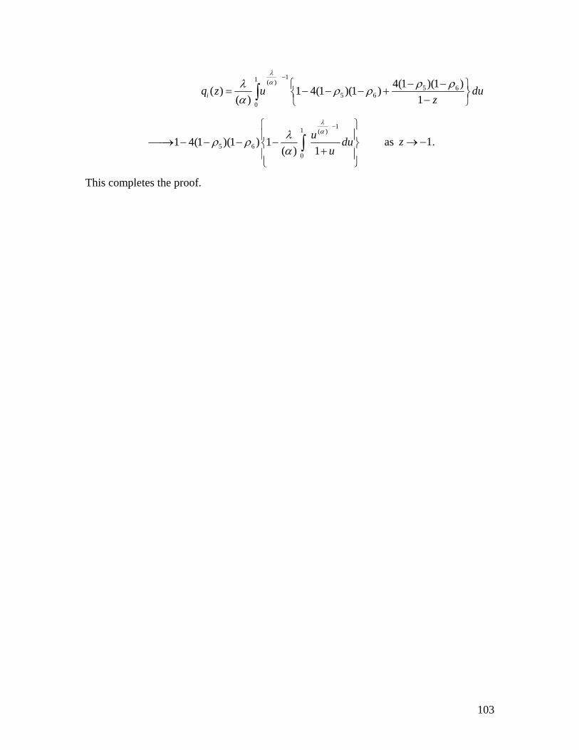
103
11 ( )
5 65 6
0
4(1 )(1 )( ) 1 4(1 )(1 )( ) 1iq z u du
z
λα ρ ρλ ρ ρ
α
−− −⎧ ⎫= − − − +⎨ ⎬−⎩ ⎭∫
11 ( )
5 60
1 4(1 )(1 ) 1( ) 1
u duu
λαλρ ρ
α
−⎧ ⎫⎪ ⎪⎯⎯→ − − − −⎨ ⎬+⎪ ⎪⎩ ⎭
∫ as 1.z →−
This completes the proof.
104
Conclusions This thesis is composed of five chapters in which the research have been carried out. We
give here necessary and useful information about these chapters.
The observation and analysis of chapters are summarized as follows.
(i) In first chapter we summarized basic definitions and results from the
Geometric Function Theory which are used in subsequent chapters.
(ii) In chapter 2 which is the main chapter of our thesis, we define some new class
( , )kB α β of analytic functions and we present its relationships with the
previously known classes. We studied the relation between the class В ( , )k α β
and kR , the class of functions of bounded radius rotation. Particularly we have
shown the inclusion relationships among the classes В ( , ),k α β kR , and
1 1В ( , ).k α β We also established a beautiful criterion of univalance for the
class В ( , )k α β for particular value of .k Further we derived arc lengths
problems for the class В ( , )k α β and as a consequence of it we established the
growth of the coefficient for the class В ( , )k α β by specializing the parameter
0.α > The behavior of Barnardi integral operator has been studied for the
class В (0, ).k β By using the concept of Gauss hypergeometric function we
have discussed in details the sharp bounds of the functions in class 2В ( , )α β
for 0α ≠ and 0 1.β< < At the end of this chapter we also derive covering
and distortion theorems for the classes 2В ( , )α β and В (1, )k β and В (1, )k β
by restricting the parameters ,k α and β .
(iii) Chapter 3 is about the new class ,,В ( , , , ),p a c A Bλ μα of analytic functions. we
studied this class by using the method of differential subordination. Many of
the known results also follows as particular cases from our results, see for
example [45, 79, 91, 103,121]. We investigate a number of inclusion
relationships for
105
the class ,,В ( , , , ).p a c A Bλ μα We have shown that the class ,1
,В ( , , , )p a c A Bλα is
closed under convolution and the generalized Livingston-Libra-Bernardi
operator defined by (1.5.5), see [43] belongs to this class. At the end of this
chapter we established distortion theorems for this class, the lower and upper
bounds of μλ
⎟⎟⎠
⎞⎜⎜⎝
⎛p
p
zzfcaI )(),(
Re for the functions in this class and some other
interesting properties of p-valent functions which are defined by means of a
certain linear operator ( , ).pI a cλ
(iv) In chapter 4, we define a new class ,, ( , , , )pN a c A Bλ μα of analytic functions. This
new class generalizes the class of non-Bazilevic functions. In this chapter, we
are primarily concerned with presenting some generalization and applications
of the class of p-valent non-Bazilevic functions. Several known results also
follows as particular cases from our results; see [78, 115, 118]. We established
a number of inclusion relationships for the class ,, ( , , , ).pN a c A Bλ μα we derive
distortion theorems for the class ,, ( , , , )pN a c A Bλ μα , the lower and upper bounds
of μ
λ ⎟⎟⎠
⎞⎜⎜⎝
⎛
)(),(Re
zfcaIz
p
p
for ,,( ) ( , , , ),pf z N a c A Bλ μα∈ and some other interesting
properties of p-valent functions which are defined here by means of a certain
linear integral operator ( , ) ( ).pI a c f zλ
(v) Chapter 5, is composed of two types of problems. The first type is concerned
with P-valent functions and the second type is concerned with meromorphic
functions. We introduce certain new subclass 1( , , , , , )kT p q sλ α ρ of P-valent
analytic functions defined by Dziok-Srivastava operator in the unit disc E . In
first part of this chapter we obtain a number of new applications for this class
of p-valent functions. We investigate a number of inclusion relationships and
derive a sharp radius problem for the class 1( , , , , , )kT p q sλ α ρ . We also
showed that the class 1( , , , , , )kT p q sλ α ρ is closed under Hadamard product
106
and we also investigated some other interesting properties of p-valent
functions which are defined by means of a certain linear integral operator
, , 1( ).p q sH α
In the second part of this chapter, two new classes ( , , , , )kMB q sα λ ρ and
( , , , , )kMT q sα λ ρ of meromorphic functions are defined by using a
meromorphic analogue of the Choi-Saigo-Srivastava operator for the
generalized hypergeometric function in the punctured unit disk E∗ .We prove
sharp radius theorem and we investigate the integral preserving behavior for
the class ( , , , , )kMB q sα λ ρ .At the end of this chapter, we have shown the two
function classes ( , , , , )kMB q sα λ ρ and ( , , , , )kMT q sα λ ρ are closed under
convolution. All the results obtained in this chapter are new
107
References
[1] M. Abramowitz and S. A. Stegun (Editors), Handbook of Mathematical
Formulas, Graphs, and Mathematical Tables, pp. 429-446, Dover, New York,
(1971).
[2] J. W. Alexander, Functions which map the interior of the unit circle upon simple
regions, Ann. Math. 17 (1915-16), 12-22.
[3] M. K. Aouf, On a class of meromorphic multivalent functions with positive
coe fficients, Math. Japon. 35 (1990), 603 − 608.
[4] M. K. Aouf, A generalization of meromorphic multivalent functions with positive
coefficients, Math. Japon. 35 (1990), 609 − 614.
[5] M. K. Aouf, H. M. Hossen and H. E. Ellatar, A certain class of meromorphic
multivalent function with positive and fixed second coefficients, Punjab Univ. J.
Math. 33 (2000), 115 − 124.
[6] F. G. Avhadiev and L. A. Aksent’ev, Function of the Bazilevic class in a disc
and in an annulus, Dokl. Akad. Nauk SSSR 214(1974), 241- 244.
[7] I. E. Bazilevic, On a case of integrability in quadratures of the Löewner-Kufarev
equation, Math. Sb. 37 (1995), 471 − 476.
[8] E. D. Belokolos, A. I. Bobenko, V. Z. Enolskii and its A R, Algebro-Geometric
Approach to non-linear integrable equations (New York: Springer) 1994.
[9] A. Bielecki and Z. Lewandowski, Sur un theorme concernant les fonctions
univalentes lineairement accessible de M. biernacki, Ann. Polon. Math. 12
(1962), 61 − 63.
108
[10] M. Biernacki, Sur la representation conforme des domaines lineairement
accessibles, Prac. Math. Fiz. 44 (1936), 293 − 314.
[11] D. A. Brannan, On functions of bounded boundary rotation, Proc. Edin. Math.
Soc. (1968-1969), 339-347.
[12] D. A. Brannan, J. G. Clunie and W. E. Kirwan, On the coefficient
problem for functions of bounded boundary rotation, Ann. Acad. Sci. Fenn. A.
I. 523 (1973), 1-18 (18 pp).
[13] B. C. Carlson and D. B. Shaffer, Starlike and prestarlike hypergeometric
functions, SIAM J. Math. Anal.159 (1984), 737-745.
[14] N. E. Cho, The Noor integral operator and strongly close-to-convex functions,
J. Math. Anal. Appl., 238 (2003), 202 − 212.
[15] N. E. Cho and I. H. Kim, Inclusion properties of certain classes of
meromorphic functions associated with the generalized hypergeometric
functions, Appl. Math. Comput. 187 (2007), 115 -121.
[16] N. E. Cho, O. S. Kown and H. M. Srivastava, Inclusion relationships and
argument properties for certain subclasses of multivalent functions associated
with a family of linear operators, J. Math. Anal. App. 292 (2004), 470 − 483.
[17] J. H. Choi, M. Siago and H. M. Srivastava, Some inclusion properties of a
certain family of integral operators, J. Math. Anal. Appl. 276 (2002),
432 − 445.
[18] N. E. Cho, O. H. Kown and H. M. Srivastava, Inclusion and argument
properties for certain subclasses of meromorphic functions associated with a
family of multiplier transformations, J. Math. Anal. Appl. 300 (2004),
505 − 520.
109
[19] J. Clunie and Ch. Pommerenke, On the coefficient of close-to-convex univalent
functions, J. Lond. Math. Soc. 41 (1966), 161-165.
[20] H. B. Coonce and M. R. Ziegler, functions with bounded Mocanu variation,
Rev. Roum. Math. Pures Appl. 19 (1974), 1093−1104.
[21] P. L. Duren, Univalent functions, Grundlehren der Math. Wissenchaften,
Springer-Verlag, New York-Berlin, 1983.
[22] J. Dziok, and H. M. Srivastava, Classes of analytic functions associated with the
generalized hypergeometric function, Appl. Math. Comput, 103 (1999), 1 −13.
[23] J. Dziok, and H. M. Srivastava, Certain subclasses of analytic functions
associated with the generalized hypergeometric function, Integral Trans. Spec.
Funct. 14 (2003), 7 −18.
[24] J. Dziok, and H. M. Srivastava, Some subclasses of analytic functions with
fixed argument of coefficients associated with the generalized hypergeometric
functions, Adv. Stud. Contemp. Math. 5 (2002), 115 −125.
[25] A. S. Focas and L-Y. Sung, Generalized Fourier Transforms, their
nonlinearization and the imaging of the brain Not. Am. Math. Soc. 52 (2005),
1178 − 1192.
[26] A. Gangadharan, T. N. Shanmugam, and H. M. Srivastava, Generalized
hypergeometiric functions associated with k-uniformly convex functions,
Comput. Math. Appl. 44 (2002), 1515−1526.
[27] R. M. Goel and N. S. Sohi, A new criterion for p-valent functions, Proc.
Amer. Math. Soc. 78 (1980), 353 − 357.
[28] A. W. Goodman, Univalent Functions, Vol. I & II, polygonal Publishing
House, Washington, New Jersey, 1983.
110
[29] A. W. Goodman, On close-to-convex functions of higher order, univ. Sci.
Budapest. Eotves. Sect. Mathematica, 15 (1972), 17−30. [30 ] G. Hergoltz, Uber potenzreiher mit positirem, reelen Teil Im einheitskreis, S. –
B. SăChs, Akad. Wiss. Leipzig Math. –Natur. KI., 63(1911) 501-511.
[31] W. Janowski, Some extremal problems for certain families of analytic functions.
I, Ann. Polon. Math. 28 (1973), 297−326.
[32] S. B. Joshi and M. K. Aouf, Meromorphic multivalent functions with positive
and fixed second coefficients, Kyungpook Math. J. 35 (1995), 163 − 169.
[33] S. B. Joshi and H. M. Srivastava, A certain familyof meromorphically
multivalent functions Comput Math. Appl. 38(3-4) (1999), 201 − 211.
[34] M. Kaku, Introduction to superstring and M-Theory (Graduate text in
contemporary physics) (New York; Springer), 1999
[35] W. Kaplan, Close-to-convex Schlicht functions, Mich. Math. J. 1 (1952),
169 −185.
[36] V. Karunakaran and K. Padma, Functions of bounded radius rotation, Indian J.
Pure Appl. Math. 12 (1981), 621 − 627.
[37] Y. C. Kim, and H. M. Srivastava, Fractional integral and other linear operators
associated with the Gaussian hypergeometric function, Complex variables
Theory Appl. 34 (1997), 293-312.
[38] P. Koebe, Uber die uniformisiesrung beliebiger analytischeer kurven, Nach.
Ges. Wiss. Gottingen, (1907), 191-210
[39] P. P. Kufarev, On one parameter families of analytic functions (in Russian)
Mat. Sb. 13 (1943), 87−118. .
111
[40] Z. Lewandowski, Sur l’identité de certain classes de functions univalence (I),
Ann. Univ. Mariae Curie-skl. Sect. A. 12(1958), 131−145.
[41] Z. Lewandowski, Sur l’identité de certain classes de functions univalence (II),
Ann. Univ. Mariae Curie-skl. Sect. A. 14 (1960), 131−145.
[42] E. Lindelöf, Mémoire sur certaines inégalitis dans la théorie des functions
monogénses et sur quelques propriétés nouvelles de ces fonctions dans le
voisinage d’un point singulier essentiel, Ann. Soc. Sci. Fenn. 35 (1909), no. 7,
1 − 35.
[43] J. E. Littlewood, On inequalities in the theory of functions, Proc. London Math.
Soc. (2) 23 (1925), 481 − 519.
[44] J. E. Littlewood, Lectures on the Theory of Functions, Oxford University
Press, Oxford and London, 1944.
[45] M. Liu, On certain subclasses of p-valent functions, Soocho. J. Math., 26: 2
(2000), 163 − 171.
[46] J. L. Liu, Strongly starlike functions associated with the Dziok − Srivastava
operator, Tamkang J. Math. 35 (2004), 37-42.
[47] J. L. Liu, The Noor integral and strongly starlike functions, J. Math. Anal.
Appl. 261 (2001), 441 −447.
[48] J. L. Liu, and H. M. Srivastava, Classes of meromorphically multivalent
functions associated with the generalized hypergeometric function, Math.
Comput. Modelling 39 (2004), 21-34.
[49] J. L. Liu and H. M. Srivastava, A linear operator and associated families of
meromorphically multivalent functions, J. Math. Anal. Appl. 259 (2001),
566 −581.
112
[50] J. L. Liu and H. M. Srivastava, Certain properties of the Dzoik −Srivastava
operator, Appl. Math. Comput. 159 (2004), 485 −493.
[51] J. L. Liu and K. I. Noor, Some properties of Noor integral operator, J.
Natur. Geom. 21 (2002), 81 − 90.
[52] K. Löwner, Üntersuchungen über die verzerrung bei konformen Abbildungen
des Eingeitschkreises 1, z < die durch Functionen mit nicht verschwindender
Ableingtung geliefert warden, Leip. Ber. 69 (1917), 89-106.
[53] K. Löwner, Üntersuchungen über schilicht konforme Abbildungen des
Einheitschkreises, I, Math. Ann. 89 (1923), 103−121.
[54] T. H. MacGregor, Radius of univalence of certain analytic functions, Proc.
Amer. Math. Soc. 14 (1963), 514 − 520.
[55] S. S. Miller, Differential inequalities and Caratheodory functions, Bull. Amer.
Math. Soc. 81 (1975), 79 − 81.
[56] S. S. Miller, The Hardy class of a Bazilevic function and its derivative, Proc.
Amer. Math. Soc. 30 (1971), 125−132.
[57] S. S. Miller and P. T. Mocanu, and M. O. Reade, All α− convex functions
are univalent and starlike, Proc. Amer. Math. Soc. 37 (1973), 552 − 554.
[58] S. S. Miller and P. T. Mocanu, Differential subordinations and univalent
functions, Michigan Math. J. 28 (1981), 157 − 171.
[59] S. S. Miller and P. T Mocanu, Differential Subordination: Theory and
Applications, in: Mongraphs and Textbooks in Pure and applied Mathematics,
vol. 225, Marcel Dekker, New York, 2000.
[60] P. T. Mocanu, Une propriete de convexite generalisee dans la theorie de la
representation conforme, Mathematica (Cluj) 11 (1969), 127-133.
113
[61] M. L. Mogra, Meromorphic multivalent functions with positive coefficients. I,
Math. Japon. 35 (1) (1990), 1 − 11.
[62] M. L. Mogra, Meromorphic multivalent functions with positive coefficients. II,
Math. Japon. 35 (6) (1990), 1089 − 1098.
[63] R. Nevanlinna, Über die Konforme Abbildund Sterngebieten, Oversikt av
Finska-Vetenskaps Societen Forhandlingar 63 (A) (6) (1921), 48 − 403.
[64] K. I. Noor and S. Al-Bani, On Bazilevic functions, Internat. J. Math and
Math. Sci., 10 (1987), 79−88.
[65] K. I. Noor, On some subclasses of functions with bounded radius and bounded
boundary rotation Pan Amer. Math. J. 6 (1) (1996), 1—7.
[66] K. I. Noor, On some integral operators fro certain families of analytic
functions, Tamkang. J. Math. 22 (1991)
[67] K. I. Noor, On some analytic functions defined by a multiplier
transformation, Internat. J. Math and Math. Sci. (2007), 1−9.
[68] K. I. Noor, Some classes of p-analytic functions defined by certain integral
operator, Mathematical inequalities and Applications, 9 (2006), 117−123.
[69] K. I. Noor, Some classes of p-valent analytic functions defined by certain
integral operator, Appl. Math. Compute. 157 (2004), 835 − 840.
[70] K. I. Noor, On new classes of integral operator, J. Nat. Geo, 16 (1999),
71- 80.
[71] K. I. Noor, On some univalent integral operators, J. Math. Anal. and Appl.
28 (1987), 586 − 592.
114
[72] K. I. Noor, On subclasses of close-to-convex functions of higher order,
Internat. J. Math. and Math Sci., 15 (1992), 279 −290.
[73] K. I. Noor and M. A. Noor, On certain classes of analytic functions
defined by Noor integral operator, J. Math. Appl. 281 (2003), 244 − 252.
[74] K. I. Noor and M. A. Noor, On integral operators, J. Math. Anal.
Appl., 238 (1999), 341−352.
[75] K. I. Noor and S. Al-Bani, On functions related to functions of bounded
Mocanu variation, Car. J. Math. 4 (1987), 53 − 65.
[76] K. I. Noor and Ali Muhammad, On analytic functions with generalized bounded mocanu variation, Appl. Math. Comput. 196 (2008), 802-811. [77] K. Noshiro, On the theory of Schlicht functions, J. Fac. Sci. Hokkaido Univ.
2 (1934-35), 129-155. Obrock, A. E.
[78] M. Obradovic, A class of univalent functions, Hokkaido Math. J., 27 (2)
(1998), 329 − 355.
[79] S. Owa and M. Obradovic, Certain subclasses of Bazilevic function of type
α, Internat. J. Math. and Math. Sci., 9: 2 (1986), 97 − 105.
[80] S. Owa and H. M. Srivastava, univalent and starlike generalized
hypergeometric functions, canad. J. Math. 39 (1987), 1057 −1077.
[81] S. Owa, H. E. Darwish and M. K. Aouf, Meromorphic multivalent
functions with positive and fixed second coefficients, Math. Japon. 46 (2)
(1997), 231−236.
[82] K. S. Padmanabhan and R. Parvatham, properties of a class of functions
with bounded boundary rotation, Ann.Polon.Math.31 (1975), 311−323.
115
[83] V. Paatero, Über Gebiete von beschränkter Randdrehung, Ann Acad. Sci.
Fenn. Ser. A 37 no 9 (1933), 20pp.
[84] V. Paatero, Über die konforme Abbildung von Gebieten, deren Ränder von
beschränkter Drehung sind. Ann. Acad. Sci. Fenn. Ser. A, 33 (1931), no. 9,
77pp.
[85] D. Ž. Pashkouleva, The starlikeness and spiral-convexity of certain subclasses
of analytic functions, in: H. M. Srivastava and S. Owa (Editors), Current Topics
in Analytic Function Theory, pp, 266 −273, World Scientific publishing
Company, Singapore, New Jersey, London and Hong Kong, 1992.
[86] J. Patel, N. E. Cho and H. M. Srivastava, Certain subclasses of multivalent
functions associated with a family of linear operators, Math. Comput. Modelling
43 (2006), 320−338.
[87] B. Pinchuk, Functions with bounded boundary rotation, Isr. J. Math., 10 (1971),
7 − 16.
[88] Ch. Pommerenke, Über die Subordination analytischer Function, J. Reine
Angew. Math. 218 (1965), 159 −173.
[89] Ch. Pommerenke, Univalent Functions, Vanderhoeck and Ruprecht, Gottengen,
1975.
[90] S. Ponnusamy, Differential subordination and Bazilevic functions, Proc. Ind.
Acad. Sci. 105 (1995), 169 −186.
[91] S. Ponnusamy and S. Rajaskaran, New sufficient conditions for starlike and
univalent functions , Soocho. J. Math., 21 : 2 (1995), 193 − 201.
116
[92] D. V. Prokorhov, A generalization of a class of close-to-convex functions (in
Russian), Matm. Zametki 11 (1972), 509−516.
[93] R. K. Raina and H. M. Srivastava, A new class of meromorphically
multivalent functions, Math. Comput. Modelling 43 (2006), 350 − 356.
[94] M. S. Robertson, On the theory of univalent functions, Ann. Math. 37 (1936),
374−408.
[95] W. Rogosinski, On the coefficients of subordinations, Proc. London Math. Soc.
(2) 48 (1945), 48 − 82.
[96] W. Rogosinski, On subordination functions, Proc. Cambridge Philos. Soc. 35
(1939), 1−26.
[97] F. Ronning, PC-fractions and Szego polynomials associated with starlike
univalent functions, Number. Algorithms 3 (1992), 383 − 392.
[98] S. Ruscheweyh, New criteria for univalent functions, Proc. Amer. Math. Soc.
49 (1975), 109−115.
[99] H. Saitoh, A Linear operator and its applications of first order differential
subordinations, Math. Japon. 44 (1996), 31 − 38.
[100] K. Sakaguchi, A note on P-valent functions, J. Math. Soc. Japan 14 (1962),
312 − 321.
[101] T. Shiel-Small, On Bazilevic functions, Quart. J. Math. 23 (1972), 135 − 142.
[102] E. M. Silvia, Subclasses of close-to-convex functions, Int. J. Math and
Math. Sci. 6 (1983), 449 −458.
[103] R. Singh, On Bazilevic functions, Proc. Amer. Math. Sci ., 38 (1973),
261 − 267.
117
[104] R. Singh and S. Singh , Convolution properties of a class of starlike
functions, Proc. Amer. Math. Soc. 108, (1989), 145 − 152.
[105] H. M. Srivastava and S. Owa (Eds), Univalent functions, Fractional Calculus,
and their Applications, Halsted Press, Ellis Horwood limited, Chichester, John
Wiley and Sons, New York, 1989.
[106] H. M. Srivastava and S. Owa (Eds), Current topics in Analytic Function
Theory, World Scientific Publishing Company, Singapore, New Jersey, London
and Hong Kong 1992.
[107] H. M. Srivastava and S. Owa, Some applications of the generalized
hypergeometric function involving certain subclasses of analytic functions,
Publ. Math. Debrecen 34 (1987), 299 − 306.
[108] H. M. Srivastava and S. Owa, Some characterization and distortion
theorems involving fractional calculus, generalized hypergeometric functions,
Hadamard products, linear operators, and certain subclasses of analytic
functions, Nagoya Math. J. 106 (1987), 1 −28.
[109] H. M. Srivastava, H. M. Hossen and M. K. Aouf, A unified presentation of
some classes of meromorphically multivalent functions, Comput Math. Appl.
38 (1999), 63 − 70.
[110] E. Strohhacker, Beitrage Zur Theorie der Schlichten Funktionen, Math. Zeit.
37(1933), 356-380.
[111] E. Study, Konforme Abbildung Einfachzusammenhangender Bereiche, B. C.
Teubner, Leipzig und Berlin, 1913.
[112] O. Tammi, On the maximization of the coefficients of Schlicht and related
functions, Ann, Acad. Sci. Fenn. Ser. AI, Math. Phys 114 (1952), 51 pp.
118
[113] K. C. Tarabicka, J. Godula and E. Zlotkiewicz, On a class of Bazilevic
functions, Ann Univ. Marie Curie-Sklodowska 33 (5) (1979), 45 − 56.
[114] D. K. Thomas, On Bazilevic functions, Trans. Amer. Math. Soc. 132
(1968), 353 −361.
[115] N. Tuneski and M. Darus, Fekete Szego − functional for non-Bazilevic
functions, Acta Mathematica. Academiae Paedagogicae. Nyiregyhaziensis, 18
(2002), 63 − 65.
[116] B. A. Uralegaddi and M. D. Ganigi, Meromorphic multivalent functions with
positive coefficients, Nepali Math. Sci. Rep. 11 (2) (1986), 95 − 102.
[117] B. A. Uralegaddi and C. Somanatha, Certain classes of meromorphic
multivalent functions, Tamkang J. Math. 23 (1992), 223 − 231.
[118] Z. Wang, C. Gao and M. Lio, On certain generalized class of Non-Bazilevic
functions, Acta Mathematica. Academiae Paedagogicae. Nyiregyhaziensis 21
(2005), 147 − 154.
[119] S. E. Warschawski, On the higher derivatives at the boundary in conformal
mapping, Trans. Amer. Math. Soc., 38 (1935), 310-340.
[120] E. T. Whittaker and G. N. Watson, A course on Modern Analysis: An
introduction to the general Theory of Infinite processes and of Analytic
Functions; With an account of the principle of Transcendental Functions, 4th
Edition, Cambridge University Press, Cambridge, 1927.
[121] D. G. Yang, Properties of certain classes of multivalent functions, Bull.
Inst. Math. Acad. Sinica, 22: 4 (1994), 361 − 367.
[122] D. G. Yang, On new subclasses of meromorphic p-valent functions, J. Math.
Res. Exposition 15(1995), 7 − 13.
119
[123] J. Zamorski, On Bazilevic Schlicht functions, Ann. Polon. Math. 12
(1962), 83 − 90.