Sometimes, Money Does Grow On Trees:

Data-Driven Demand Response With DR-Advisor

Madhur Behl and Rahul MangharamDepartment of Electrical and Systems Engineering

University of PennsylvaniaPA, USA

{mbehl, rahulm}@seas.upenn.edu

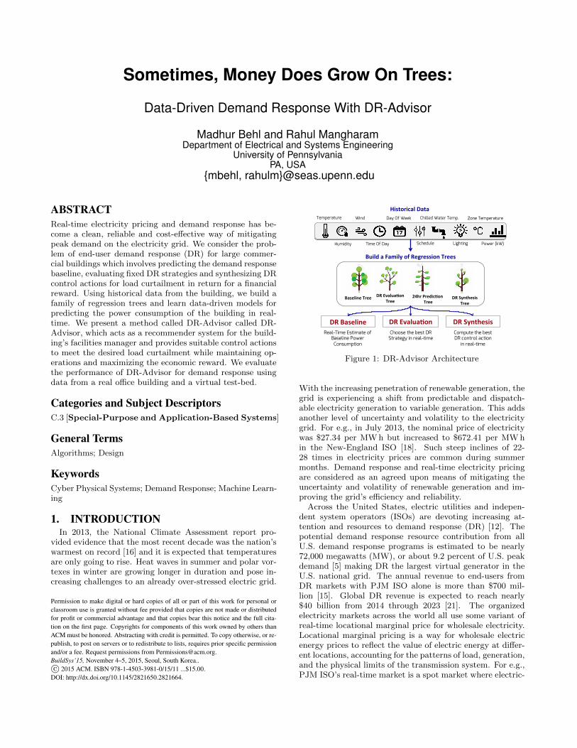
ABSTRACTReal-time electricity pricing and demand response has be-come a clean, reliable and cost-effective way of mitigatingpeak demand on the electricity grid. We consider the prob-lem of end-user demand response (DR) for large commer-cial buildings which involves predicting the demand responsebaseline, evaluating fixed DR strategies and synthesizing DRcontrol actions for load curtailment in return for a financialreward. Using historical data from the building, we build afamily of regression trees and learn data-driven models forpredicting the power consumption of the building in real-time. We present a method called DR-Advisor called DR-Advisor, which acts as a recommender system for the build-ing’s facilities manager and provides suitable control actionsto meet the desired load curtailment while maintaining op-erations and maximizing the economic reward. We evaluatethe performance of DR-Advisor for demand response usingdata from a real office building and a virtual test-bed.

Categories and Subject DescriptorsC.3 [Special-Purpose and Application-Based Systems]

General TermsAlgorithms; Design

KeywordsCyber Physical Systems; Demand Response; Machine Learn-ing

1. INTRODUCTIONIn 2013, the National Climate Assessment report pro-

vided evidence that the most recent decade was the nation’swarmest on record [16] and it is expected that temperaturesare only going to rise. Heat waves in summer and polar vor-texes in winter are growing longer in duration and pose in-creasing challenges to an already over-stressed electric grid.

Permission to make digital or hard copies of all or part of this work for personal orclassroom use is granted without fee provided that copies are not made or distributedfor profit or commercial advantage and that copies bear this notice and the full cita-tion on the first page. Copyrights for components of this work owned by others thanACM must be honored. Abstracting with credit is permitted. To copy otherwise, or re-publish, to post on servers or to redistribute to lists, requires prior specific permissionand/or a fee. Request permissions from Permissions@acm.org.BuildSys’15, November 4–5, 2015, Seoul, South Korea..c© 2015 ACM. ISBN 978-1-4503-3981-0/15/11 ...$15.00.

DOI: http://dx.doi.org/10.1145/2821650.2821664.

Temperature

Humidity

Wind

Time Of Day

Day Of Week

Schedule

Chilled Water Temp.

Lighting Power (kW)

Zone Temperature

Historical  Data  

Baseline  Tree   DR  Evalua4on  Tree  

DR  Synthesis  Tree  

24hr  Predic4on    Tree  

Build  a  Family  of  Regression  Trees  

DR  Baseline   DR  Evalua4on   DR  Synthesis  Real-Time Estimate of

Baseline Power Consumption

Choose the best DR Strategy in real-time

Compute the best DR control action

in real-time

Figure 1: DR-Advisor Architecture

With the increasing penetration of renewable generation, thegrid is experiencing a shift from predictable and dispatch-able electricity generation to variable generation. This addsanother level of uncertainty and volatility to the electricitygrid. For e.g., in July 2013, the nominal price of electricitywas $27.34 per MW h but increased to $672.41 per MW hin the New-England ISO [18]. Such steep inclines of 22-28 times in electricity prices are common during summermonths. Demand response and real-time electricity pricingare considered as an agreed upon means of mitigating theuncertainty and volatility of renewable generation and im-proving the grid’s efficiency and reliability.

Across the United States, electric utilities and indepen-dent system operators (ISOs) are devoting increasing at-tention and resources to demand response (DR) [12]. Thepotential demand response resource contribution from allU.S. demand response programs is estimated to be nearly72,000 megawatts (MW), or about 9.2 percent of U.S. peakdemand [5] making DR the largest virtual generator in theU.S. national grid. The annual revenue to end-users fromDR markets with PJM ISO alone is more than $700 mil-lion [15]. Global DR revenue is expected to reach nearly$40 billion from 2014 through 2023 [21]. The organizedelectricity markets across the world all use some variant ofreal-time locational marginal price for wholesale electricity.Locational marginal pricing is a way for wholesale electricenergy prices to reflect the value of electric energy at differ-ent locations, accounting for the patterns of load, generation,and the physical limits of the transmission system. For e.g.,PJM ISO’s real-time market is a spot market where electric-

ity prices are calculated at five-minute intervals based on thegrid operating conditions.

Electricity costs are the one of the largest components of alarge commercial and industrial (C&I) building’s operatingbudget. This is because, such customers are often subjectto peak-demand based electricity pricing. In this pricingpolicy, a customer is charged not only for the amount ofelectricity it has consumed but also for its peak demandover the billing cycle. High peak loads also lead to a highercost of production and distribution of electricity. Therefore,these peaks are not only operationally inefficient but alsoextremely expensive for both the utilities and the end-users.Furthermore, the volatility and variance in real-time elec-tricity rates poses a risk for large buildings [1]. They needthe capability to respond to the price volatility in a fast andreliable manner. Such customers are increasingly looking todemand response programs to help manage their electricitycosts. DR programs involve a voluntary response of a build-ing to real-time price signals. In such programs, end-usersreduce their electricity load during periods of high prices orupon receiving a DR request from the utility and receive afinancial reward for their load curtailment.

There are four barriers to successfully enabling real-timebuilding electricity prediction and demand response: (a) Eachbuilding is designed and used in a different way and there-fore, it has to be uniquely modeled. Learning high fidelitypredictive models of buildings using first principles basedapproaches is very cost and time prohibitive and requiresretrofitting the building with several sensors [22]; (b) Sec-ondly, the building’s operating conditions, internal thermaldisturbances and environmental conditions must be takeninto account to make appropriate DR decisions, which isnot possible with rule-based and pre-determined demand re-sponse strategies since they do not account for the state ofthe building but are instead based on best practicies andrules of thumbs. (c) Thirdly, upon receiving a notificationfor a DR event, the building’s facilities manager must de-termine an appropriate DR strategy to achieve the requiredload curtailment. These control strategies can include ad-justing zone temperature set-points, supply air temperatureand chilled water temperature set-point, dimming or turn-ing off lights, decreasing duct static pressure set-points andrestricting the supply fan operation etc.. In a large build-ing, it is difficult to asses the effect of one control actionon other sub-systems and on the building’s overall powerconsumption because the building sub-systems are tightlycoupled. (d) Lastly, predictive models for buildings, regard-less how sophisticated, can effectively be rendered powerlessunless they can be interpreted by human experts. For e.g.,artificial neural networks (ANN) obscure physical controlknobs and hence, are difficult to interpret by building fa-cilities managers. Therefore, the required solution must betransparent, human centric and highly interpretable.

We present a method called DR-Advisor (Demand Response-Advisor), which acts as a recommender system for the build-ing’s facilities manager and provides the power consump-tion prediction and control actions for meeting the requiredload curtailment and maximizing the economic reward. Us-ing historical meter and weather data along with set-pointand schedule information, DR-Advisor builds a family ofinterpretable regression trees to learn non-parametric data-driven models for predicting the power consumption of thebuilding (Figure 1). DR-Advisor can be used for real-time

Time

Dem

and

RAMP

SUSTAINEDRESPONSE

RECOV-ERY

Notification ReductionDeadline

Release Resume

Strategy 1Strategy 2Strategy 3

. . .Strategy N

21

1

i j km

OptionsEstimate Baseline Demand

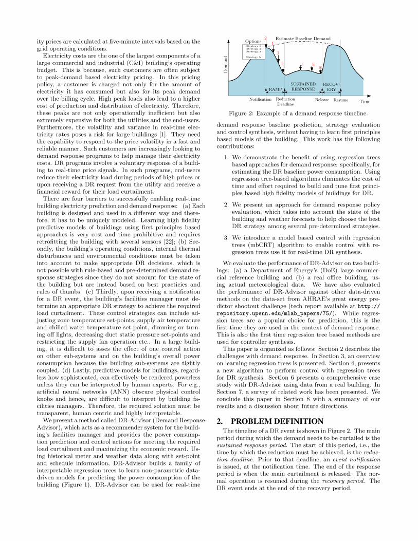
Figure 2: Example of a demand response timeline.

demand response baseline prediction, strategy evaluationand control synthesis, without having to learn first principlesbased models of the building. This work has the followingcontributions:

1. We demonstrate the benefit of using regression treesbased approaches for demand response: specifically, forestimating the DR baseline power consumption. Usingregression tree-based algorithms eliminates the cost oftime and effort required to build and tune first princi-ples based high fidelity models of buildings for DR.

2. We present an approach for demand response policyevaluation, which takes into account the state of thebuilding and weather forecasts to help choose the bestDR strategy among several pre-determined strategies.

3. We introduce a model based control with regressiontrees (mbCRT) algorithm to enable control with re-gression trees use it for real-time DR synthesis.

We evaluate the performance of DR-Advisor on two build-ings: (a) a Department of Energy’s (DoE) large commer-cial reference building and (b) a real office building, us-ing actual meteorological data. We have also evaluatedthe performance of DR-Advisor against other data-drivenmethods on the data-set from AHRAE’s great energy pre-dictor shootout challenge (tech report available at http://

repository.upenn.edu/mlab_papers/75/). While regres-sion trees are a popular choice for prediction, this is thefirst time they are used in the context of demand response.This is also the first time regression tree based methods areused for controller synthesis.

This paper is organized as follows: Section 2 describes thechallenges with demand response. In Section 3, an overviewon learning regression trees is presented. Section 4, presentsa new algorithm to perform control with regression treesfor DR synthesis. Section 6 presents a comprehensive casestudy with DR-Advisor using data from a real building. InSection 7, a survey of related work has been presented. Weconclude this paper in Section 8 with a summary of ourresults and a discussion about future directions.

2. PROBLEM DEFINITIONThe timeline of a DR event is shown in Figure 2. The main

period during which the demand needs to be curtailed is thesustained response period. The start of this period, i.e., thetime by which the reduction must be achieved, is the reduc-tion deadline. Prior to that deadline, an event notificationis issued, at the notification time. The end of the responseperiod is when the main curtailment is released. The nor-mal operation is resumed during the recovery period. TheDR event ends at the end of the recovery period.

We focus on three challenging problems of end-user de-mand response, which are described next.

2.1 DR baseline predictionThe DR baseline is an estimate of the electricity that

would have been consumed by a customer in the absenceof a demand response event. The measurement and verifi-cation of the demand response baseline is the most criticalcomponent of any DR program. The baseline is the primarytool for measuring curtailment during a DR event, and de-termining financial paybacks. DR-Advisor utilizes histori-cal power meter and weather data to estimate the baselinepower consumption in real-time during a DR event.

2.2 DR strategy evaluationUpon receiving a notification for a DR event, the build-

ing’s facilities manager must choose a control strategy amongseveral pre-determined strategies to achieve the required powercurtailment level. Each strategy includes adjusting tempera-ture set-points, lighting levels and temporarily switching offequipment, such as escalators, and plug loads to differentlevels across different time intervals. As only one strategycan be use at a time, the question then is, how to choose theDR strategy from a pre-determined set of strategies whichleads to the largest load curtailment ?

In Fig. 2, there are N different strategies available tochoose from. DR-Advisor predicts the power consumptionof the building due to each strategy at every time-step andchooses the DR strategy which leads to the largest load cur-tailment.

2.3 DR strategy synthesisInstead of choosing a DR strategy from a pre-determined

set of strategies, one may ask how to synthesize new DRstrategies ? For example, in the traditional rule-based ap-proaches, determined by prior curtailment experiments andoperator experience, the zone temperature set-points of thebuilding should be increased to pre-determined levels to re-duce the cooling load. However, based on the state of thebuilding and environmental conditions of the current day,it is unclear by how much and for how long the particu-lar rule-based curtailment will comply to the curtailmentrequirements? This is the problem of demand response syn-thesis because we want to synthesize optimal control actionswhich are suitable for the DR event based on the currentstate of the building, outside weather and real-time electric-ity prices.

2.4 Rule-based and model-based DRThe two most popular approaches to respond to DR in-

clude rule based and model based DR strategies. In a rulebased DR strategy, different levels of curtailment are achievedby following a pre-programmed strategy. Fixed DR strate-gies have the advantage of being simple but they do notaccount for the state of the building and weather condi-tions during a DR event. Despite this lack of predictability,rule-based DR strategies account for the majority of DRapproaches.

Model based DR involves mathematically modeling thebuilding in order to predict the overall power consumptionand take actions based on the predicted response. Creatingand learning such high fidelity models (e.g., with Energy-Plus [7]) is extremely cost and time prohibitive [22]. The

user expertise, time, and associated costs required to developa model of a single building is very high. This is because usu-ally a building modeling domain expert will use a softwaretool to create the geometry of a building from the buildingdesign, add detailed information about material properties,about equipment and operational schedules. There is al-ways a gap between the modeled and the real building andthe domain expert must manually tune the model to matchmeasured data [17].

The goal with data-driven methods, such as with DR-Advisor, is to make the best of both worlds; i.e. simplicity ofrule based approaches and the predictive capability of modelbased strategies, but without the expense of first principleor grey-box model development.

3. LEARNING REGRESSION TREESData driven modeling consists of obtaining a functional

model that relates the value of the response variable Y withthe values of the predictor variables X1, X2, · · · , Xm. Forexample in linear regression, a linear form is assumed for theunknown function and the parameters of the model are esti-mated using a least squares criterion. Predictors like linearor polynomial regression are global models, where a singlepredictive formula is assumed to hold over the entire dataspace. When the data has lots of features which interactin complicated, nonlinear ways, assembling a single globalmodel can be difficult, lead to poor response predictions andhopelessly confusing when you do succeed.

An approach to non-linear regression is to partition thedata space into smaller regions, where the interactions aremore manageable. We then partition the partitions again;this is called recursive partitioning, until finally we get tochunks of the data space which are so tame that we can fitsimple models to them. Therefore, the global model has twoparts: the recursive partition, and a simple model for eachcell of the partition. Regression trees belong to the classof recursive partitioning algorithms. The seminal algorithmfor learning regression trees is CART as described in [4]. Formore details on how regression trees are built, we direct thereader to Appendix A.

3.1 Boosting and random forestsThe problem with regression trees is that they can have

high variance and can sometimes overfit the data. It is theprice to be paid for estimating a simple model. While prun-ing and cross validation can help reduce over fitting, we canalso use ensemble methods for growing more stable trees.DR-Advisor uses two ensemble methods for building powerprediction: boosted regression trees and random forests.

The goal of ensemble methods is to combine the predic-tions of several base estimators built with a given learningalgorithm in order to improve generalizability and robust-ness over a single estimator. Random forests or tree-baggingare a type of ensemble method which makes predictions byaveraging over the predictions of several independent basemodels. The essential idea is to average many noisy but ap-proximately unbiased trees, and hence reduce the variance.Injecting randomness into the tree construction can happenin many ways. The choice of which dimensions to use as splitcandidates at each leaf can be randomized, as well as thechoice of coefficients for random combinations of features.For a more comprehensive review of random forests we re-fer the reader to [3]. In boosting, trees are fitted iteratively

Xd1

Xc1

Xc2

Xd2 Xd2

Xd3

YR1 = β0,1 + βT1 X

YRi = β0,i + βTi X

R1

Ri

Tree Depth

Xd1

Xc1

Xd2

Xc2

Xd3

Mix

OfControllableandUncontrollableFeatures

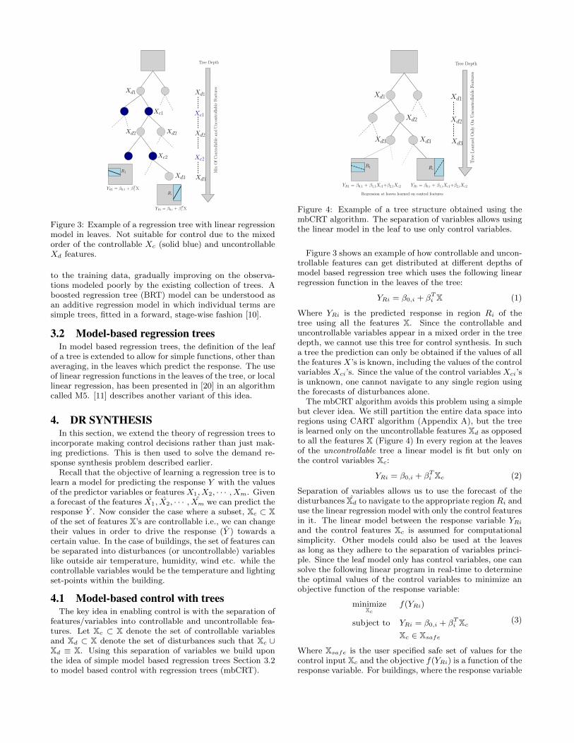
Figure 3: Example of a regression tree with linear regressionmodel in leaves. Not suitable for control due to the mixedorder of the controllable Xc (solid blue) and uncontrollableXd features.

to the training data, gradually improving on the observa-tions modeled poorly by the existing collection of trees. Aboosted regression tree (BRT) model can be understood asan additive regression model in which individual terms aresimple trees, fitted in a forward, stage-wise fashion [10].

3.2 Model-based regression treesIn model based regression trees, the definition of the leaf

of a tree is extended to allow for simple functions, other thanaveraging, in the leaves which predict the response. The useof linear regression functions in the leaves of the tree, or locallinear regression, has been presented in [20] in an algorithmcalled M5. [11] describes another variant of this idea.

4. DR SYNTHESISIn this section, we extend the theory of regression trees to

incorporate making control decisions rather than just mak-ing predictions. This is then used to solve the demand re-sponse synthesis problem described earlier.

Recall that the objective of learning a regression tree is tolearn a model for predicting the response Y with the valuesof the predictor variables or features X1, X2, · · · , Xm. Givena forecast of the features X1, X2, · · · , Xm we can predict theresponse Y . Now consider the case where a subset, Xc ⊂ Xof the set of features X’s are controllable i.e., we can changetheir values in order to drive the response (Y ) towards acertain value. In the case of buildings, the set of features canbe separated into disturbances (or uncontrollable) variableslike outside air temperature, humidity, wind etc. while thecontrollable variables would be the temperature and lightingset-points within the building.

4.1 Model-based control with treesThe key idea in enabling control is with the separation of

features/variables into controllable and uncontrollable fea-tures. Let Xc ⊂ X denote the set of controllable variablesand Xd ⊂ X denote the set of disturbances such that Xc ∪Xd ≡ X. Using this separation of variables we build uponthe idea of simple model based regression trees Section 3.2to model based control with regression trees (mbCRT).

Xd1

Xd2

Xd3

YR1 = β0,1 + β1,1Xc1+β2,1Xc2

R1 Ri

Tree Depth

Xd1

Xd2

Xd3

TreeLearned

Only

OnUncontrollableFeatures

Xd3

YRi = β0,i + β1,iXc1+β2,iXc2

Regression at leaves learned on control features

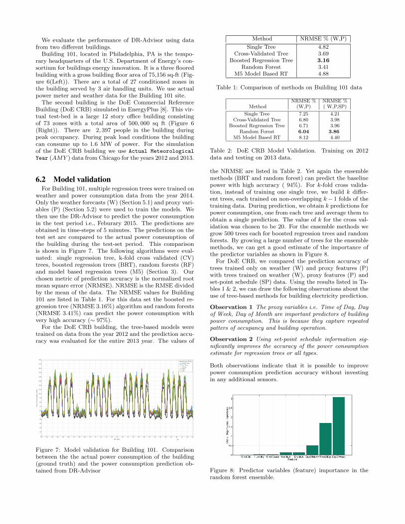
Figure 4: Example of a tree structure obtained using thembCRT algorithm. The separation of variables allows usingthe linear model in the leaf to use only control variables.

Figure 3 shows an example of how controllable and uncon-trollable features can get distributed at different depths ofmodel based regression tree which uses the following linearregression function in the leaves of the tree:

YRi = β0,i + βTi X (1)

Where YRi is the predicted response in region Ri of thetree using all the features X. Since the controllable anduncontrollable variables appear in a mixed order in the treedepth, we cannot use this tree for control synthesis. In sucha tree the prediction can only be obtained if the values of allthe features X’s is known, including the values of the controlvariables Xci’s. Since the value of the control variables Xci’sis unknown, one cannot navigate to any single region usingthe forecasts of disturbances alone.

The mbCRT algorithm avoids this problem using a simplebut clever idea. We still partition the entire data space intoregions using CART algorithm (Appendix A), but the treeis learned only on the uncontrollable features Xd as opposedto all the features X (Figure 4) In every region at the leavesof the uncontrollable tree a linear model is fit but only onthe control variables Xc:

YRi = β0,i + βTi Xc (2)

Separation of variables allows us to use the forecast of thedisturbances Xd to navigate to the appropriate region Ri anduse the linear regression model with only the control featuresin it. The linear model between the response variable YRi

and the control features Xc is assumed for computationalsimplicity. Other models could also be used at the leavesas long as they adhere to the separation of variables princi-ple. Since the leaf model only has control variables, one cansolve the following linear program in real-time to determinethe optimal values of the control variables to minimize anobjective function of the response variable:

minimizeXc

f(YRi)

subject to YRi = β0,i + βTi Xc

Xc ∈ Xsafe

(3)

Where Xsafe is the user specified safe set of values for thecontrol input Xc and the objective f(YRi) is a function of theresponse variable. For buildings, where the response variable

is power consumption, the objective function can denote thefinancial reward of minimizing the power consumption.

Algorithm 1 mbCRT: Model Based Control With Regres-sion Trees

1: Design Time2: procedure Model Training3: Separation of Variables4: Set Xc ← Controllable Features5: Set Xd ← Uncontrollable Features6: Build the uncontrollable tree Tmrt with Xd

7: for all Regions Ri at the leaves of Tmrt do8: Fit linear model YRi = β0,i + βT

i Xc

9: end for10: end procedure11: Run Time12: procedure Control Synthesis13: At time t obtain forecast Xd(t + 1) of disturbances

Xd1(t+ 1), Xd2(t+ 1), · · ·14: Using Xd(t+ 1) determine the leaf and region Rrt

15: for Region Rrt do16: Solve optimization in Eq3 for optimal control ac-

tion X∗c(t)17: end for18: end procedure

The intuition behind the mbCRT Algorithm 1 is that atrun time t, we use the forecast Xd(t+ 1) of the disturbancefeatures to determine the region of the uncontrollable treeand hence, the linear model to be used for the control. Wethen solve the simple linear program corresponding to thatregion to obtain the optimal values of the control variables.

5. DATA DESCRIPTIONIn order to build a regression tree which can predict the

power consumption of the building, we need to train on time-stamped historical data. The data that we use can be di-vided into three different categories as described below:

5.1 Weather dataWeather data includes measurements of the outside tem-

perature, relative humidity, wind characteristics and solarirradiation at the building site.

5.2 Schedule dataUsing time-stamp information in the building power con-

sumption data, we create proxy variables which correlatewith repeated patterns of electricity consumption e.g., dueto occupancy or equipment schedules.

1. Day of Week: This is a categorical predictor whichtakes values from 1 − 7 depending on the day of theweek. This variable can partition the data space onpatterns which occur on specific days of the week.For instance, there could a big auditorium in an of-fice building which is only used on certain days.

2. Weekends and Holidays: For most buildings theequipment schedule and occupancy patterns changesignificantly over weekends and holidays. Weekends,special days and holidays are represented by a singlebinary predictor which takes the values {1,−1}.

Figure 5: MATLAB GUI for DR-Advisor

3. Time of Day: This is quite an important predictoras it can adequately capture daily patterns in powerconsumption due to occupancy, lighting and applianceuse without directly measuring any one of them.

Besides using proxy schedule predictors, actual buildingschedules can also be used as training data for building thetrees. The prime candidate for obtaining actual schedulesare temperature set-points schedules of chilled water sup-ply, supply air temperature and zone air temperature onthe HVAC side and lighting schedules. Using actual scheduleinformation can greatly improve the accuracy of the powerconsumption prediction as we shall see later.

5.3 Building dataLastly, since we are trying to predict the power consump-

tion of the building, we require historical time-stamped powerconsumption (or meter) data. The power consumption isthe response variable of the regression tree i.e., the vari-able which we want to predict. The state of the building isrequired for DR strategy evaluation and synthesis. This in-cludes (i) Chilled Water Supply Temperature (ii) Hot WaterSupply Temperature (iii) Zone Air Temperature (iv) SupplyAir Temperature (v) Lighting levels

6. CASE STUDYDR-Advisor (Figure 5) is being developed into a toolbox

(http://mlab.seas.upenn.edu/dr-advisor/). DR-Advisoris also compared against other data-driven methods on thedata-set from AHRAE’s great energy predictor shootoutchallenge (tech report available at http://repository.upenn.edu/mlab_papers/75/). In this section, we present a com-prehensive case study to show how DR-Advisor can be usedto address the three demand response challenges (Section 2).

6.1 Building description

Figure 6: Left: Building 101 in Philadelphia; Right: 3Drendering of the DoE commercial reference building in En-ergyPlus.

We evaluate the performance of DR-Advisor using datafrom two different buildings.

Building 101, located in Philadelphia, PA is the tempo-rary headquarters of the U.S. Department of Energy’s con-sortium for buildings energy innovation. It is a three flooredbuilding with a gross building floor area of 75,156 sq-ft (Fig-ure 6(Left)). There are a total of 27 conditioned zones inthe building served by 3 air handling units. We use actualpower meter and weather data for the Building 101 site.

The second building is the DoE Commercial ReferenceBuilding (DoE CRB) simulated in EnergyPlus [8]. This vir-tual test-bed is a large 12 story office building consistingof 73 zones with a total area of 500, 000 sq ft (Figure 6(Right)). There are 2, 397 people in the building duringpeak occupancy. During peak load conditions the buildingcan consume up to 1.6 MW of power. For the simulationof the DoE CRB building we use Actual Meteorological

Year (AMY ) data from Chicago for the years 2012 and 2013.

6.2 Model validationFor Building 101, multiple regression trees were trained on

weather and power consumption data from the year 2014.Only the weather forecasts (W) (Section 5.1) and proxy vari-ables (P) (Section 5.2) were used to train the models. Wethen use the DR-Advisor to predict the power consumptionin the test period i.e., Feburary 2015. The predictions areobtained in time-steps of 5 minutes. The predictions on thetest set are compared to the actual power consumption ofthe building during the test-set period. This comparisonis shown in Figure 7. The following algorithms were eval-uated: single regression tree, k-fold cross validated (CV)trees, boosted regression trees (BRT), random forests (RF)and model based regression trees (M5) (Section 3). Ourchosen metric of prediction accuracy is the normalized rootmean square error (NRMSE). NRMSE is the RMSE dividedby the mean of the data. The NRMSE values for Building101 are listed in Table 1. For this data set the boosted re-gression tree (NRMSE 3.16%) algorithm and random forests(NRMSE 3.41%) can predict the power consumption withvery high accuracy (∼ 97%).

For the DoE CRB building, the tree-based models weretrained on data from the year 2012 and the prediction accu-racy was evaluated for the entire 2013 year. The values of

01 02 03 04 05 06 07 08 09 10 11 12 13 14 15 16 17 18 19 20 21 22 23 24 25 26 27 28 01

·105

0

10

20

30

40

50

60

70

80

90

100

110

120

130

140

150

160

170

180

Feb 2015

Pow

erConsumption(kW

)

Ground TruthSingle TreeCV TreeForestBRTM5

Figure 7: Model validation for Building 101. Comparisonbetween the the actual power consumption of the building(ground truth) and the power consumption prediction ob-tained from DR-Advisor

Method NRMSE % (W,P)

Single Tree 4.82Cross-Validated Tree 3.69

Boosted Regression Tree 3.16Random Forest 3.41

M5 Model Based RT 4.88

Table 1: Comparison of methods on Building 101 data

MethodNRMSE %

(W,P)NRMSE %( W,P,SP)

Single Tree 7.25 4.21Cross-Validated Tree 6.80 3.98

Boosted Regression Tree 6.71 3.96Random Forest 6.04 3.86

M5 Model Based RT 8.12 4.40

Table 2: DoE CRB Model Validation. Training on 2012data and testing on 2013 data.

the NRMSE are listed in Table 2. Yet again the ensemblemethods (BRT and random forest) can predict the baselinepower with high accuracy ( 94%). For k-fold cross valida-tion, instead of training one single tree, we build k differ-ent trees, each trained on non-overlapping k− 1 folds of thetraining data. During prediction, we obtain k predictions forpower consumption, one from each tree and average them toobtain a single prediction. The value of k for the cross val-idation was chosen to be 20. For the ensemble methods wegrow 500 trees each for boosted regression trees and randomforests. By growing a large number of trees for the ensemblemethods, we can get a good estimate of the importance ofthe predictor variables as shown in Figure 8.

For DoE CRB, we compared the prediction accuracy oftrees trained only on weather (W) and proxy features (P)with trees trained on weather (W), proxy features (P) andset-point schedule (SP) data. Using the results listed in Ta-bles 1 & 2, we can draw the following observations about theuse of tree-based methods for building electricity prediction.

Observation 1 The proxy variables i.e. Time of Day, Dayof Week, Day of Month are important predictors of buildingpower consumption. This is because they capture repeatedpatters of occupancy and building operation.

Observation 2 Using set-point schedule information sig-nificantly improves the accuracy of the power consumptionestimate for regression trees or all types.

Both observations indicate that it is possible to improvepower consumption prediction accuracy without investingin any additional sensors.

Figure 8: Predictor variables (feature) importance in therandom forest ensemble.

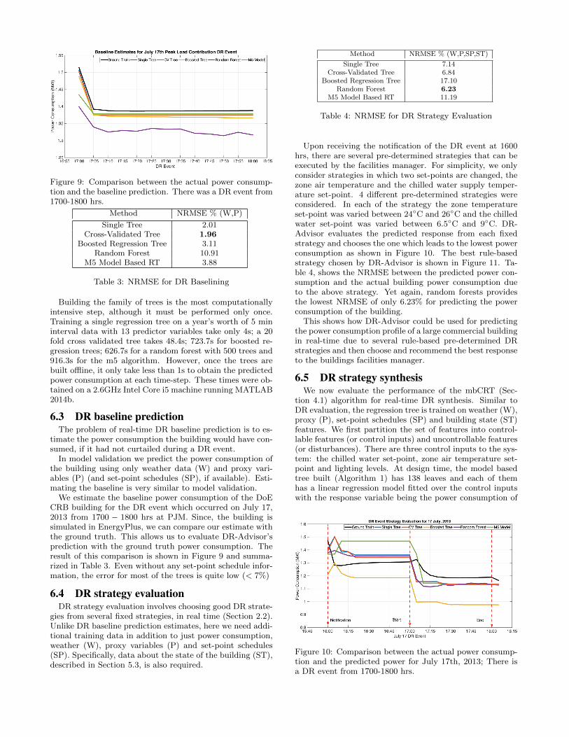
Figure 9: Comparison between the actual power consump-tion and the baseline prediction. There was a DR event from1700-1800 hrs.

Method NRMSE % (W,P)

Single Tree 2.01Cross-Validated Tree 1.96

Boosted Regression Tree 3.11Random Forest 10.91

M5 Model Based RT 3.88

Table 3: NRMSE for DR Baselining

Building the family of trees is the most computationallyintensive step, although it must be performed only once.Training a single regression tree on a year’s worth of 5 mininterval data with 13 predictor variables take only 4s; a 20fold cross validated tree takes 48.4s; 723.7s for boosted re-gression trees; 626.7s for a random forest with 500 trees and916.3s for the m5 algorithm. However, once the trees arebuilt offline, it only take less than 1s to obtain the predictedpower consumption at each time-step. These times were ob-tained on a 2.6GHz Intel Core i5 machine running MATLAB2014b.

6.3 DR baseline predictionThe problem of real-time DR baseline prediction is to es-

timate the power consumption the building would have con-sumed, if it had not curtailed during a DR event.

In model validation we predict the power consumption ofthe building using only weather data (W) and proxy vari-ables (P) (and set-point schedules (SP), if available). Esti-mating the baseline is very similar to model validation.

We estimate the baseline power consumption of the DoECRB building for the DR event which occurred on July 17,2013 from 1700 − 1800 hrs at PJM. Since, the building issimulated in EnergyPlus, we can compare our estimate withthe ground truth. This allows us to evaluate DR-Advisor’sprediction with the ground truth power consumption. Theresult of this comparison is shown in Figure 9 and summa-rized in Table 3. Even without any set-point schedule infor-mation, the error for most of the trees is quite low (< 7%)

6.4 DR strategy evaluationDR strategy evaluation involves choosing good DR strate-

gies from several fixed strategies, in real time (Section 2.2).Unlike DR baseline prediction estimates, here we need addi-tional training data in addition to just power consumption,weather (W), proxy variables (P) and set-point schedules(SP). Specifically, data about the state of the building (ST),described in Section 5.3, is also required.

Method NRMSE % (W,P,SP,ST)

Single Tree 7.14Cross-Validated Tree 6.84

Boosted Regression Tree 17.10Random Forest 6.23

M5 Model Based RT 11.19

Table 4: NRMSE for DR Strategy Evaluation

Upon receiving the notification of the DR event at 1600hrs, there are several pre-determined strategies that can beexecuted by the facilities manager. For simplicity, we onlyconsider strategies in which two set-points are changed, thezone air temperature and the chilled water supply temper-ature set-point. 4 different pre-determined strategies wereconsidered. In each of the strategy the zone temperatureset-point was varied between 24◦C and 26◦C and the chilledwater set-point was varied between 6.5◦C and 9◦C. DR-Advisor evaluates the predicted response from each fixedstrategy and chooses the one which leads to the lowest powerconsumption as shown in Figure 10. The best rule-basedstrategy chosen by DR-Advisor is shown in Figure 11. Ta-ble 4, shows the NRMSE between the predicted power con-sumption and the actual building power consumption dueto the above strategy. Yet again, random forests providesthe lowest NRMSE of only 6.23% for predicting the powerconsumption of the building.

This shows how DR-Advisor could be used for predictingthe power consumption profile of a large commercial buildingin real-time due to several rule-based pre-determined DRstrategies and then choose and recommend the best responseto the buildings facilities manager.

6.5 DR strategy synthesisWe now evaluate the performance of the mbCRT (Sec-

tion 4.1) algorithm for real-time DR synthesis. Similar toDR evaluation, the regression tree is trained on weather (W),proxy (P), set-point schedules (SP) and building state (ST)features. We first partition the set of features into control-lable features (or control inputs) and uncontrollable features(or disturbances). There are three control inputs to the sys-tem: the chilled water set-point, zone air temperature set-point and lighting levels. At design time, the model basedtree built (Algorithm 1) has 138 leaves and each of themhas a linear regression model fitted over the control inputswith the response variable being the power consumption of

Figure 10: Comparison between the actual power consump-tion and the predicted power for July 17th, 2013; There isa DR event from 1700-1800 hrs.

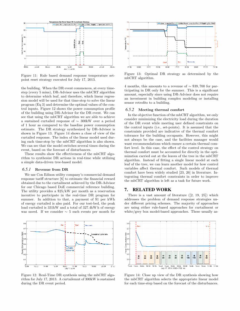
Figure 11: Rule based demand response temperature set-point reset strategy executed for July 17, 2013.

the building. When the DR event commences, at every time-step (every 5 mins), DR-Advisor uses the mbCRT algorithmto determine which leaf, and therefore, which linear regres-sion model will be used for that time-step to solve the linearprogram (Eq 3) and determine the optimal values of the con-trol inputs. Figure 12 shows the power consumption profileof the building using DR-Advisor for the DR event. We cansee that using the mbCRT algorithm we are able to achievea sustained curtailed response of ∼ 300kW over a periodof 1 hour as compared to the baseline power consumptionestimate. The DR strategy synthesized by DR-Advisor isshown in Figure 13. Figure 14 shows a close of view of thecurtailed response. The index of the linear model used dur-ing each time-step by the mbCRT algorithm is also shown.We can see that the model switches several times during theevent, based on the forecast of disturbances.

These results show the effectiveness of the mbCRT algo-rithm to synthesize DR actions in real-time while utilizinga simple data-driven tree-based model.

6.5.1 Revenue from DR

We use Con Edison utility company’s commercial demandresponse tariff structure [6] to estimate the financial rewardobtained due to the curtailment achieved by the DR-Advisorfor our Chicago based DoE commercial reference building.The utility provides a $25/kW per month as a reservationincentive to participate in the real-time DR program forsummer. In addition to that, a payment of $1 per kWhof energy curtailed is also paid. For our test-bed, the peakload curtailed is 331kW and a total of 327.4kW h of energywas saved. If we consider ∼ 5 such events per month for

Figure 12: Real-Time DR synthesis using the mbCRT algo-rithm for July 17, 2013. A curtailemnt of 300kW is sustainedduring the DR event period.

Figure 13: Optimal DR strategy as determined by thembCRT algorithm.

4 months, this amounts to a revenue of ∼ $39, 700 for par-ticipating in DR only for the summer. This is a significantamount, especially since using DR-Advisor does not requirean investment in building complex modeling or installingsensor retrofits to a building.

6.5.2 Meeting thermal comfort

In the objective function of the mbCRT algorithm, we onlyconsider minimizing the electricity load during the durationof the DR event while meeting user defined constraints onthe control inputs (i.e., set-points). It is assumed that theconstraints provided are indicative of the thermal comforttolerance for the building occupants. However, this mightnot always be the case, and the facilities manager wouldwant recommendations which ensure a certain thermal com-fort level. In this case, the effect of the control strategy onthermal comfort must be accounted for directly in the opti-mization carried out at the leaves of the tree in the mbCRTalgorithm. Instead of fitting a single linear model at eachleaf of the tree, we can learn another model for how controlvariables affect thermal comfort. Such models of thermalcomfort have been widely studied [23, 26] in literature. In-tegrating thermal comfort constraints in order to improvethe mbCRT algorithm is left as a task for future work.

7. RELATED WORKThere is a vast amount of literature ([2, 19, 25]) which

addresses the problem of demand response strategies un-der different pricing schemes. The majority of approachesare using either rule-based approaches for curtailment orwhite/grey box model-based approaches. These usually as-

Figure 14: Close up view of the DR synthesis showing howthe mbCRT algorithm selects the appropriate linear modelfor each time-step based on the forecast of the disturbances.

sume that the model of the system is either perfectly knownor found in literature, whereas the task is much more com-plicated and time consuming in case of a real building andsometimes, it can be even more complex and involved thanthe controller design itself. After several years of work on us-ing first principles based models for demand response, mul-tiple authors [22, 28] have concluded that the biggest hurdleto mass adoption of intelligent building control is the costand effort required to capture accurate dynamical modelsof the buildings. Since DR-Advisor only learns an aggre-gate building level model and combined with the fact thatweather forecasts are expected to become cheaper; there islittle to no additional sensor cost of implementing the DR-Advisor recommendation system in large buildings. Thereare ongoing efforts to make tuning and identifying white boxmodels of buildings more autonomous [17]. Figuring out thecorrect response on a fast time scales (1-5 mins) using justdata-driven methods has’nt been adequately addressed be-fore and makes the DR-Advisor approach and tool novel.

Several machine learning approaches [9, 24, 27, 14] havebeen utilized before for forecasting electricity load. However,there are three significant shortcomings of the work in thisarea: (a) First, the time-scales at which the load forecastsare generated range from 15−20 min upto an hour; which istoo coarse grained for DR events which only last for at mosta couple of hours and for real-time electricity prices whichexhibit frequent changes. (b) Secondly, these approachesare not aimed at solving demand response problems but arerestricted to long term load forecasting with applicationsin evaluating building retrofits savings and building energyratings. (c) Lastly, in these methods, there is no focus oncontrol synthesis or addressing the suitability of the modelto be used in control design; whereas the mbCRT algorithmenables the use of regression trees for control synthesis withapplications in demand response.

8. CONCLUSIONDR-Advisor, a data-driven method for demand response

has been presented. It is being developed into a MATLABbased toolbox (http://mlab.seas.upenn.edu/dr-advisor/)We show how regression tree based methods provide an ex-cellent way to predict the power consumption response ofa large commercial building while being simple and inter-pretable. The use of regression trees based methods fordemand response evaluation and synthesis based challengesfor large scale commercial buildings is novel. The perfor-mance of DR-Advisor is evaluated using data from a DOEcommercial reference building and from a real office build-ing. DR-Advisor achieves a prediction accuracy of 94-97%for DR baseline and DR strategy evaluation. We presenta model based control with regression trees (mbCRT) al-gorithm which enables control synthesis using interpretabletree based structures. Using our algorithm DR-Advisor canachieve a sustained curtailment during a DR event. Usinga DR pricing structure from Con Edison utility, we esti-mate a potential revenue of ∼ $40,000 for the DoE referencebuilding over one summer. The primary advantage of DR-Advisor is that it bypasses cost and time prohibitive processof building high fidelity grey/white box models of buildings.Our ongoing work involves extending the mbCRT algorithmto account for thermal comfort and use DR-Advisor fromthe perspective of the utility company for optimal DR dis-patch. We are also extending the algorithm to operate in

a finite receding horizon manner as opposed to a one-steplook-ahead optimization.

9. ACKNOWLEDGMENTSThis work was supported in part by STARnet, a Semicon-

ductor Research Corporation program, sponsored by MARCOand DARPA and by NSF MRI-0923518 grants.

10. REFERENCES[1] Energy price risk and the sustainability of demand side supply

chains. Applied Energy, 123(0):327 – 334, 2014.

[2] D. Auslander, D. Caramagno, D. Culler, T. Jones, A. Krioukov,M. Sankur, J. Taneja, J. Trager, S. Kiliccote, R. Yin, et al.Deep demand response: The case study of the citris building atthe university of california-berkeley.

[3] L. Breiman. Random forests. Machine learning, 45(1):5–32,2001.

[4] L. Breiman, J. Friedman, C. J. Stone, and R. A. Olshen.Classification and regression trees. CRC press, 1984.

[5] F. E. R. Commission et al. Assessment of demand response andadvanced metering. 2012.

[6] Con Edison. Demand response programs details.

[7] D. B. Crawley, L. K. Lawrie, et al. Energyplus: creating anew-generation building energy simulation program. Energyand Buildings, 33(4):319 – 331, 2001.

[8] M. Deru, K. Field, D. Studer, et al. U.s. department of energycommercial reference building models of the national buildingstock. 2010.

[9] R. E. Edwards, J. New, and L. E. Parker. Predicting futurehourly residential electrical consumption: A machine learningcase study. Energy and Buildings, 49:591–603, 2012.

[10] J. Elith, J. R. Leathwick, and T. Hastie. A working guide toboosted regression trees. Journal of Animal Ecology,77(4):802–813, 2008.

[11] J. H. Friedman. Multivariate adaptive regression splines. Theannals of statistics, pages 1–67, 1991.

[12] C. Goldman. Coordination of energy efficiency and demandresponse. Lawrence Berkeley National Laboratory, 2010.

[13] T. Hastie, R. Tibshirani, J. Friedman, T. Hastie, J. Friedman,and R. Tibshirani. The elements of statistical learning,volume 2. Springer, 2009.

[14] T. Hong, W.-K. Chang, and H.-W. Lin. A fresh look at weatherimpact on peak electricity demand and energy use of buildingsusing 30-year actual weather data. Applied Energy,111:333–350, 2013.

[15] P. Interconnection. 2014 deamand response operations marketsactivity report. 2014.

[16] J. M. Melillo, T. Richmond, and G. W. Yohe. Climate changeimpacts in the united states: the third national climateassessment. US Global change research program, 841, 2014.

[17] J. R. New, J. Sanyal, M. Bhandari, and S. Shrestha. Autotunee+ building energy models. Proceedings of the 5th NationalSimBuild of IBPSA-USA, 2012.

[18] New-England ISO. Real-time maps and charts, 2013.

[19] F. Oldewurtel, D. Sturzenegger, G. Andersson, M. Morari, andR. S. Smith. Towards a standardized building assessment fordemand response. In Decision and Control (CDC), IEEE52nd Annual Conference on. IEEE, 2013.

[20] J. R. Quinlan et al. Learning with continuous classes. In 5thAustralian joint conference on artificial intelligence,volume 92, pages 343–348. Singapore, 1992.

[21] N. Research. Demand response for commercial & industrialmarkets market players and dynamics, key technologies,competitive overview, and global market forecasts. 2015.

[22] D. Sturzenegger, D. Gyalistras, M. Morari, and R. Smith.Model predictive climate control of a swiss office building:Implementation, results, and cost-benefit analysis. ControlSystems Technology, IEEE Transactions on, 2015.

[23] M. Taleghani, M. Tenpierik, S. Kurvers, and A. van denDobbelsteen. A review into thermal comfort in buildings.Renewable and Sustainable Energy Reviews, 26:201–215, 2013.

[24] A. Vaghefi, M. Jafari, E. Bisse, Y. Lu, and J. Brouwer.Modeling and forecasting of cooling and electricity loaddemand. Applied Energy, 136:186–196, 2014.

[25] P. Xu, P. Haves, M. A. Piette, and J. Braun. Peak demandreduction from pre-cooling with zone temperature reset in anoffice building. Berkeley National Laboratory, 2004.

[26] L. Yang, H. Yan, and J. C. Lam. Thermal comfort and buildingenergy consumption implications–a review. Applied Energy,115:164–173, 2014.

[27] W. Yin, Y. Simmhan, and V. K. Prasanna. Scalable regressiontree learning on hadoop using openplanet. In Proceedings ofthird international workshop on MapReduce and itsApplications Date, pages 57–64. ACM, 2012.

[28] E. Zacekova, Z. Vana, and J. Cigler. Towards the real-lifeimplementation of mpc for an office building: Identificationissues. Applied Energy, 135:53–62, 2014.

APPENDIXA. BUILDING REGRESSION TREES

We explain how regression trees are built using an exam-ple adapted from [13]. Tree-based methods partition thefeature space into a set of rectangles (more formally, hyper-rectangles) and then fit a simple model in each one. Theyare conceptually simple yet powerful. Let us consider a re-gression problem with continuous response Y and inputs X1

and X2, each taking values in the unit interval. The topleft plot of Figure 15 shows a partition of the feature spaceby lines that are parallel to the coordinate axes. In eachpartition element we can model Y with a different constant.However, there is a problem: although each partitioning linehas a simple description like X1 = k, some of the resultingregions are complicated to describe. To simplify things, wecan restrict ourselves to only consider recursive binary parti-tions, like the ones shown in the top right plot of Figure 15.We first split the space into two regions, and model the re-sponse by the mean of Y in each region. We choose thevariable and split-point to achieve the best prediction of Y .Then one or both of these regions are split into two moreregions, and this process is continued, until some stoppingrule is applied. This is the recursive partitioning part of thealgorithm. For example, in the top right plot of Figure 15,we first split at X1 = t1. Then the region X1 ≤ t1 is splitat X2 = t2 and the region X1 > t1 is split at X1 = t3.Finally, the region X1 > t3 is split at X2 = t4. The resultof this process is a partition of the data-space into the fiveregions R1, R2, · · · , R5. The corresponding regression tree

Figure 15: Top right: 2D feature space by recursive binarysplitting. Top left: partition that cannot be obtained fromrecursive binary splitting. Bottom left: tree correspondingto the partition. Bottom right: perspective plot of the pre-diction surface.

model predicts Y with a constant ci in region Ri i.e.,,

T (X) =

5∑i=1

ciI {(X1, X2) ∈ Ri} (4)

This same model can be represented by the binary treeshown in the bottom left of Figure 15. The full data-set sitsat the top or the root of the tree. Observations satisfyingthe condition at each node are assigned to the left branch,and the others to the right branch. The terminal nodes orleaves of the tree correspond to the regions R1, R2, ..., R5.

A.1 Node splitting criteriaFor regression trees we adopt the sum of squares as our

splitting criteria i.e a variable at a node will be split if it min-imizes the following sum of squares between the predictedresponse and the actual output variable.∑

(yi − T (xi))2 (5)

It is easy to see that the best response ci (from equation 4for yi from partition Ri is just the average of output samplesin the region Ri i.e

ci = avg(yi|xi ∈ Ri) (6)

Finding the best binary partition in terms of minimum sumof squares is generally computationally infeasible. A greedyalgorithm is used instead. Starting with all of the data,consider a splitting variable j and split point s, and definethe following pair of left (RL) and right (RR) half-planes

RL(j, s) = {X|Xj ≤ s} ,RR(j, s) = {X|Xj > s}

(7)

The splitting variable j and the split point s is obtained bysolving the following minimization:

minj,s

mincL

∑xi∈RL(j,s)

(yi − cL)2 + mincR

∑xi∈RR(j,s)

(yi − cR)2

(8)

where, for any choice of j and s, the inner minimization inequation 8 is solved using

cL = avg(yi|xi ∈ RL(j, s))

cR = avg(yi|xi ∈ RR(j, s))(9)

For each splitting variable Xj , the determination of the splitpoint s can be done very quickly and hence by scanningthrough all of the inputs (Xi’s), the determination of thebest pair (j, s) is feasible. Having found the best split, wepartition the data into the two resulting regions and repeatthe splitting process on each of the two regions. Then thisprocess is repeated on all of the resulting regions.

A.2 Stopping criteria and pruningEvery recursive algorithm needs to know when it’s done.

For regression trees this means when to stop splitting thenodes. A very large tree might over fit the data, while asmall tree might not capture the important structure. A pre-ferred, strategy is to grow a large tree, stopping the splittingprocess only when some minimum number of data points ata node (MinLeaf) is reached. Then this large tree is prunedusing cost-complexity pruning methods.