Embed Size (px)
Citation preview

An IMAGE Satellite Guide to Exploring the Earth’s Magnetic Field 1
An IMAGE Satellite Guide to Exploring the Earth’s Magnetic Field 2
Dr. James Burch
IMAGE PrincipalInvestigator
Dr. William Taylor
Dr. Sten Odenwald
IMAGE Education and Public OutreachRaytheon ITS and NASA Goddard SFC
IMAGE Education and Public OutreachRaytheon ITS and NASA Goddard SFC
Cover Artwork:
Image of the Earth’s ring currentobserved by the IMAGE, HENAinstrument. Some representativemagnetic field lines are shown in white.
This resource was developed bythe NASA Imager for
Magnetopause-to-Auroral GlobalExploration (IMAGE)
Information about the IMAGEMission is available at:
http://image.gsfc.nasa.govhttp://pluto.space.swri.edu/IMAGE
Resources for teachers andstudents are available at:
http://image.gsfc.nasa.gov/poetry
Ms. Annie DiMarco
Ms. Susan Higley
Mr. Bill Pine
Mr. Tom Smith
Greenwood Elementary SchoolBrookville, Maryland
Cherry Hill Middle SchoolElkton, Maryland
Chaffey High SchoolOntario, California
Briggs-Chaney Middle SchoolSilver Spring, Maryland
An IMAGE Satellite Guide to Exploring the Earth’s Magnetic Field 3
Chapter 1: What is a Magnet?
Chapter 2: Investigating Earth’s Magnetism
Chapter 3: Magnetic Storms, Aurora and Space Weather

An IMAGE Satellite Guide to Exploring the Earth’s Magnetic Field 4
X X X X X X X X X X X X X X X
X X X X X X X
X X X X X X X X X X X X X X X X X
X
X X
X X X X X X X X X X X X X X X X X X X X X
X X X X X X X X
X X X X X X X X X X X X X X X X X X X X
X X X X X X X X X X X X X X X X X X X X
X X X X X X X X X X X X X X X X X
X X X X
X X X X
1 2 3 4 5 6 7 8 9 10 11 12 13 14 15 16 17 18 19 20 21 22 23
Inquiry
Motion
Forces
Light
Electricity
Magnetism
Energy
Astronomy
Earth
Technology
Science
Human Endeavor
What is aMagnet?
Investigating the Earth’s Magnetism Magnetic Storms, Aurora andSpace Weather
This book was designed to provide teachers with activities that allow studentsto explore topics related to the Sun-Earth Connection.
We have provided a full range of activities for the grades 3-12 community sothat teachers may see how the single topic of magnetism can evolve insophistication as the student matures. Teachers are invited to use the activitiesas-is, or to modify them as needed to suit their particular objectives.
The units are designed for use in conjunction with your current curriculum asindividual lessons or as a unit. The chart above is designed to assist teachersin integrating the activities contained with existing curricula and NationalScience Standards.
Throughout the lessons you will find activities that require the students to makeobservations, and record their findings. Observations can be recorded inscience learning logs, journals or by organization into charts or graphs.

An IMAGE Satellite Guide to Exploring the Earth’s Magnetic Field 5
"Students should be actively engaged in learning to view the world scientifically. They should be encouraged to ask questions about nature and to seek answer, collect things, count
and measure things, make qualitative observations, organize collections and observationsand discuss findings."
(American Association for the Advancement of Science; Benchmarks for Science)
Scientists and students share an active curiosity about the world. A truescientist maintains that inquisitive quality and continues to question, explore andinvestigate.
In developing this book, we have attempted to stimulate an active curiosityabout the Sun-Earth Connection, and specifically how Earth and its magnetic fieldreact to solar influences. The activities in this book combine hands-onexperimentation with the use of satellite data resources on the internet, to providestudents with a well-rounded perspective into basic issues in contemporary Sun-Earth research.
"When students observe differences in the way things behave or get different results in repeated investigations, they should suspect that something differs from trial to trial, and try to find out what." (AAAS ‘Benchmarks for Science Literacy, 1999)
Each lesson focuses upon a particular aspect of studying the Sun and theEarth as a system, and how scientists make the observations. Included in theprocedure sections are questions that will further encourage scientific inquiry.
Each lesson begins with a description of the activities in which the students willparticipate, and provides general background information. The objectives sectionshighlight the science process skills the students will develop while completing theactivities. The procedures sections are general, and can be adapted to meet theknowledge and developmental levels of the students.
Many lessons have extension activities designed to have the students applythe new knowledge in grade appropriate activities.
Although the lessons may be used with only the information provided, weinclude where appropriate the addresses of web pages on the Internet, and on theIMAGE ‘Space Weather’ CDROM, so that further material can be incorporated intothe lesson. For further information, please visit the IMAGE satellite’s Education andPublic Outreach web site at:
An IMAGE Satellite Guide to Exploring the Earth’s Magnetic Field 6
An IMAGE Satellite Guide to Exploring the Earth’s Magnetic Field 7
An IMAGE Satellite Guide to Exploring the Earth’s Magnetic Field 8
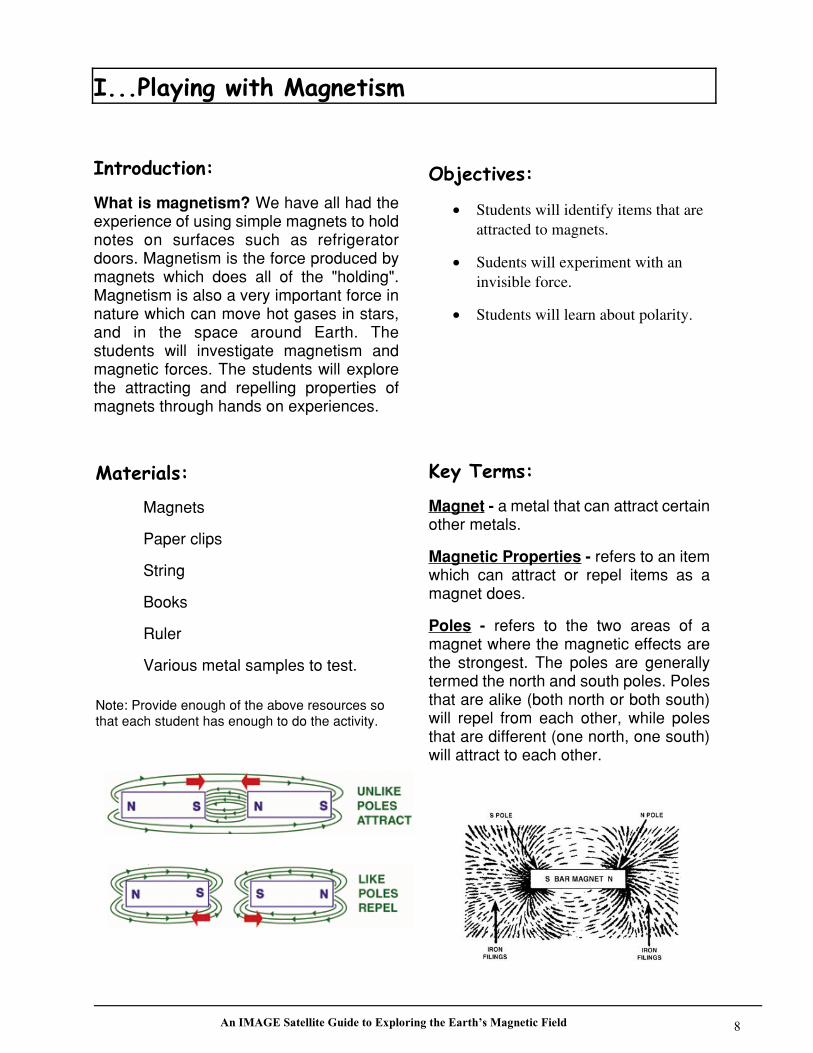
What is magnetism? We have all had theexperience of using simple magnets to holdnotes on surfaces such as refrigeratordoors. Magnetism is the force produced bymagnets which does all of the "holding".Magnetism is also a very important force innature which can move hot gases in stars,and in the space around Earth. Thestudents will investigate magnetism andmagnetic forces. The students will explorethe attracting and repelling properties ofmagnets through hands on experiences.
• Students will identify items that areattracted to magnets.
• Sudents will experiment with aninvisible force.
• Students will learn about polarity.
Magnets
Paper clips
String
Books
Ruler
Various metal samples to test.
Note: Provide enough of the above resources sothat each student has enough to do the activity.
Magnet - a metal that can attract certainother metals.
Magnetic Properties - refers to an itemwhich can attract or repel items as amagnet does.
Poles - refers to the two areas of amagnet where the magnetic effects arethe strongest. The poles are generallytermed the north and south poles. Polesthat are alike (both north or both south)will repel from each other, while polesthat are different (one north, one south)will attract to each other.

An IMAGE Satellite Guide to Exploring the Earth’s Magnetic Field 9
• Give each student a magnet. Have the students explore the metallic samples attractedto the magnet. The students should look at the samples and find commoncharacteristics. Have them fill in the table below and add their own samples. Thestudents should record their findings in a learning log.
• Tape one end of a piece of string to a desk; tie the other end onto a paper clip. Take asecond piece of string and suspend the magnet from a ruler anchored with books.Adjust the level of books so that the distance between the magnet and the paper clipallows the clip to stand up without touching the magnet. The students should see thata magnetic force could be invisible. You can place pieces of paper or cloth between theclip and the magnet to show the strength of the magnetic force. Can the students findmaterials that block magnetic forces?
• With the string still attached, have the students try to raise the paper clip from the deskwith a magnet. They should try to accomplish this without letting the magnet and paperclip touch. The students should keep a log of how they were able to accomplish this;what methods and strategies were used.
• Give each student two magnets. Allow the students time to explore the attracting andrepelling properties of magnets. They should be able to demonstrate that a magnet hastwo ends or poles that will attract or repel from other poles. Have the students observewhat happens when two magnets are repelling from each other. The students shouldfind a partner and discuss what they have seen and whether their classmate was ableto discover the same properties.
The students will learn the characteristics of magnetism. The students will demonstrate theattracting and repelling properties of magnets.
An IMAGE Satellite Guide to Exploring the Earth’s Magnetic Field 10
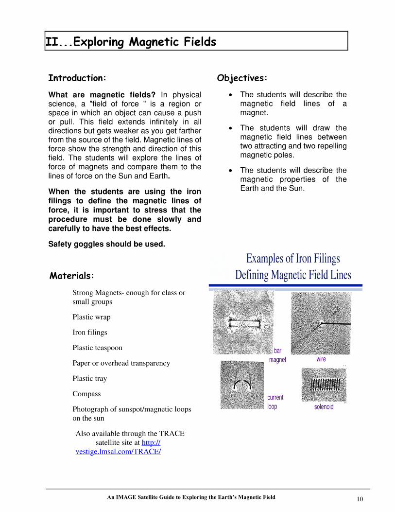
What are magnetic fields? In physicalscience, a "field of force " is a region orspace in which an object can cause a pushor pull. This field extends infinitely in alldirections but gets weaker as you get fartherfrom the source of the field. Magnetic lines offorce show the strength and direction of thisfield. The students will explore the lines offorce of magnets and compare them to thelines of force on the Sun and Earth.
When the students are using the ironfilings to define the magnetic lines offorce, it is important to stress that theprocedure must be done slowly andcarefully to have the best effects.
Safety goggles should be used.
• The students will describe themagnetic field lines of amagnet.
• The students will draw themagnetic field lines betweentwo attracting and two repellingmagnetic poles.
• The students will describe themagnetic properties of theEarth and the Sun.
Strong Magnets- enough for class or small groups
Plastic wrap
Iron filings
Plastic teaspoon
Paper or overhead transparency
Plastic tray
Compass
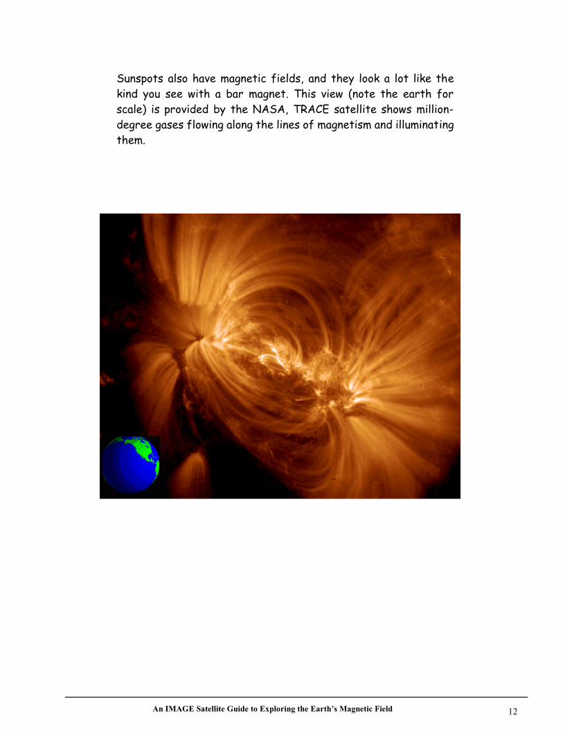
Photograph of sunspot/magnetic loops on the sun
Also available through the TRACE satellite site at http://
vestige.lmsal.com/TRACE/
An IMAGE Satellite Guide to Exploring the Earth’s Magnetic Field 11
**Caution the students that the iron filings should not be eaten or blown into eyes. **
• Cover the magnets with plastic wrap to keep the iron filings off them. Place the coveredmagnet in the plastic tray and place the paper on top. The students should carefully usethe spoon to sprinkle a small amount of the iron filings on the paper. The iron filings willstay in a pattern that indicates the lines of force of that magnet. The students shoulddraw their observations in their learning logs. After the students have completed theirobservations, the iron filings can be poured off the paper and the tray back into thecontainer.
• Give each group of students a pair of covered magnets. Place the covered magnetsabout an inch apart in the plastic tray and place the paper on top. The students shouldcarefully sprinkle a small amount of the iron filings on the paper. The iron filings will stayin a pattern that indicates the lines of force between the magnets. The students shouldlook at the lines of force and determine whether the magnetic poles are alike ordifferent. Have the students record their observations in their learning logs.
• Have the students repeat the activity of finding lines of force, but this time one of themagnets must be reversed so that its opposite pole is about an inch away from theother magnet. The students should look at the lines of force and determine whether themagnetic poles are alike or different. The students should record their observations intheir learning logs.
• Display the photograph on page 14, or the TRACE website of magnetic loops on theSun’s surface without informing the students of the source. Question the students aboutwhat they observe in the photograph. The image should resemble the magnetic lines offorce the students saw in the previous activity. The students, as scientists, shouldunderstand that they are seeing magnetic properties on the Sun. How does the patterncompare to the iron filings near a bar magnet? Answer: They should display a definite North and South polarity as well as loops. Scientists have in fact confirmed this using other observations.
• Discuss the student’s observations which were noted in their log books.
• Display a compass to the students. Explain that in the Northern Hemisphere the needleof the compass will point to the magnetic north because it is magnetized. When acompass is held on Earth, the Earth’s magnetic field exerts a force on the needle. Thisshould help the students understand that Earth also has magnetic properties. If the"north" part of a compass is attracted to the magnetic north pole of Earth, what is thepolarity of the Earth's north magnetic pole? Answer - South!
The students will gain an understanding of the presence of magnetic fields aroundmagnets, the Sun and Earth. The students will learn that the magnetic poles attractwhen they are different and repel when they are the same.
An IMAGE Satellite Guide to Exploring the Earth’s Magnetic Field 12
An IMAGE Satellite Guide to Exploring the Earth’s Magnetic Field 13
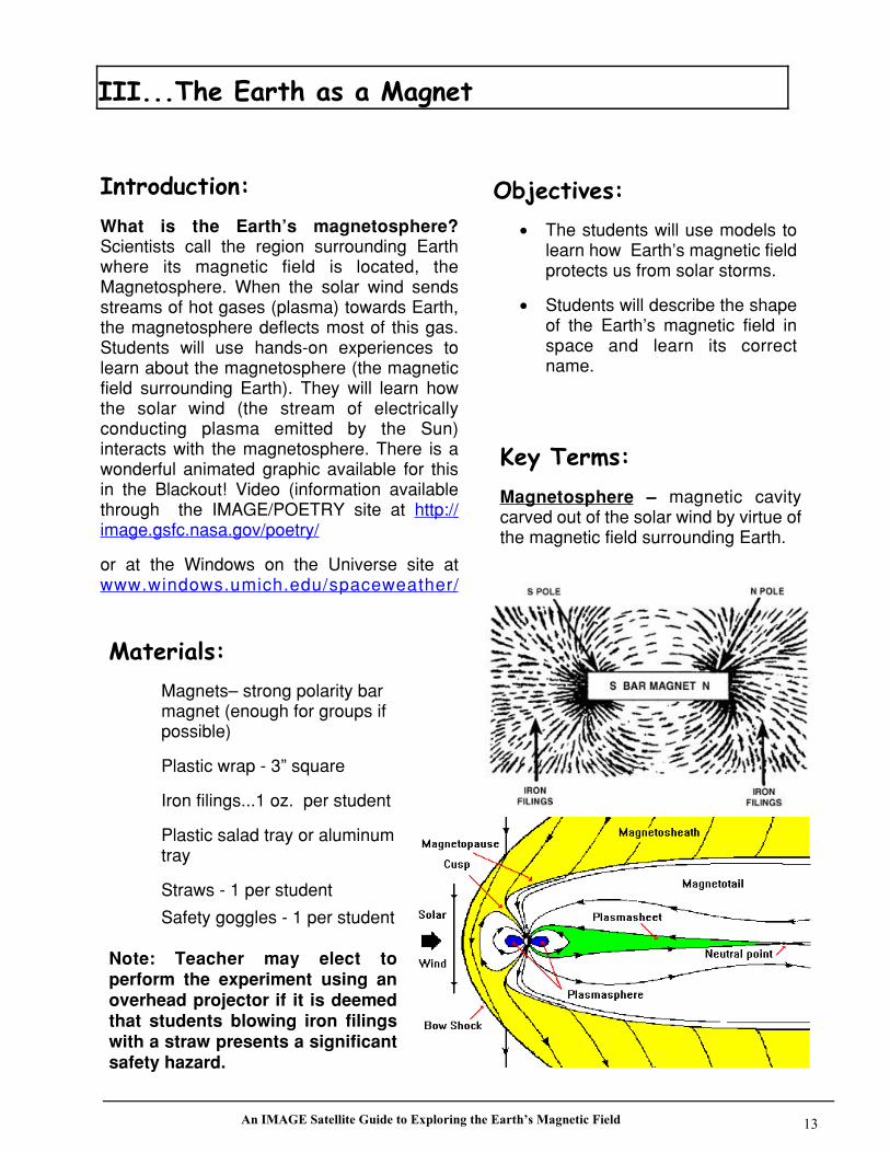
What is the Earth’s magnetosphere?Scientists call the region surrounding Earthwhere its magnetic field is located, theMagnetosphere. When the solar wind sendsstreams of hot gases (plasma) towards Earth,the magnetosphere deflects most of this gas.Students will use hands-on experiences tolearn about the magnetosphere (the magneticfield surrounding Earth). They will learn howthe solar wind (the stream of electricallyconducting plasma emitted by the Sun)interacts with the magnetosphere. There is awonderful animated graphic available for thisin the Blackout! Video (information availablethrough the IMAGE/POETRY site at http:// image.gsfc.nasa.gov/poetry/
or at the Windows on the Universe site atwww.windows.umich.edu/spaceweather/
• The students will use models tolearn how Earth’s magnetic fieldprotects us from solar storms.
• Students will describe the shapeof the Earth’s magnetic field inspace and learn its correctname.
Magnets– strong polarity bar magnet (enough for groups if possible)
Plastic wrap - 3” square
Iron filings...1 oz. per student
Plastic salad tray or aluminum tray
Straws - 1 per student
Safety goggles - 1 per student
Note: Teacher may elect toperform the experiment using anoverhead projector if it is deemedthat students blowing iron filingswith a straw presents a significantsafety hazard.
Magnetosphere – magnetic cavitycarved out of the solar wind by virtue ofthe magnetic field surrounding Earth.
An IMAGE Satellite Guide to Exploring the Earth’s Magnetic Field 14
What protects the Earth?
• Earth has a protective cover called the magnetosphere. It works as skin does on yourbody to keep out harmful things. Students can observe a model of the magnetosphereusing magnets and iron filings. To keep your bar magnet clean, wrap it in plastic wrapwith tape around it, or put contact paper around it. Place a bar magnet under a plasticsalad tray or aluminum tray. Sprinkle some iron filings onto the tray from a distance ofabout 10 inches. Observe the pattern made by the iron filings held in place by theforces between the opposite poles of the magnets. The earth’s magnetosphere can bemodeled by blowing softly through a straw towards the magnetic field lines. Asquishing of the field lines on one side of the model shows how Earth’smagnetosphere looks. Have the students draw the model of Earth’s magnetosphere intheir learning logs.
What happens when the solar wind approaches the earth’s magnetosphere?
• Students can observe the way water flows around a stone as a pattern of the solarwind as it flows around the Earth.
• Place the bar magnet under a plastic tray or aluminum tray. Place a small buttondirectly above the center of the magnet to model the Earth. Sprinkle the iron filingsalong the edge of one side of the tray covering the magnet. Softly blow the filingstoward the button through a straw. Caution the students to blow carefully so that noiron filings get into eyes or mouth! Depending on the force used in blowing, the filingswill be trapped in the magnetic lines of force. Compare this to the trapping of the solarparticles by Earth’s magnetosphere. Have the students draw the model of the effectsof the solar wind on Earth’s magnetosphere.
The students will gain an understanding of Earth’s protective region, called themagnetosphere. The students will gain an understanding of how Earth’smagnetosphere interacts with the charged plasma sent from the sun in solar wind andin solar storm events called Coronal Mass Ejections (CMEs).
An IMAGE Satellite Guide to Exploring the Earth’s Magnetic Field 15
Grades 3-5
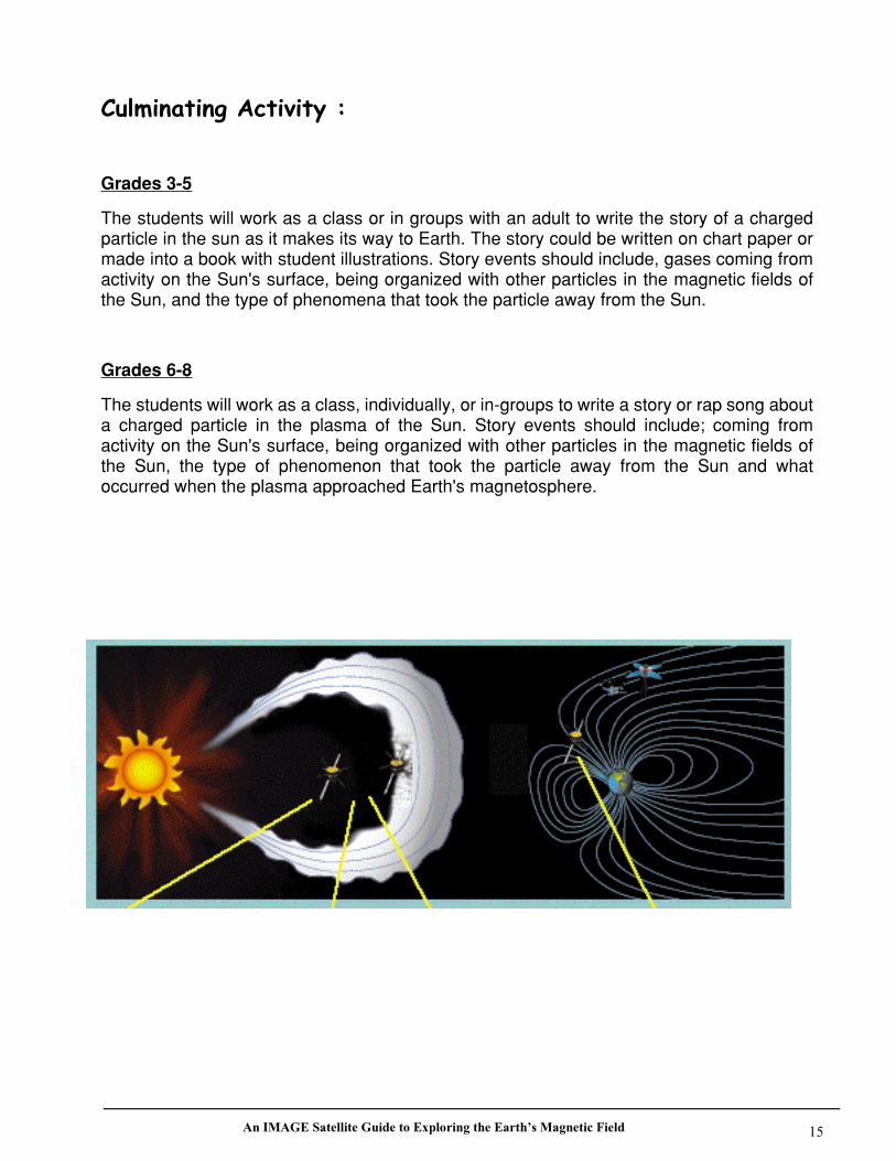
The students will work as a class or in groups with an adult to write the story of a chargedparticle in the sun as it makes its way to Earth. The story could be written on chart paper ormade into a book with student illustrations. Story events should include, gases coming fromactivity on the Sun's surface, being organized with other particles in the magnetic fields ofthe Sun, and the type of phenomena that took the particle away from the Sun.
Grades 6-8
The students will work as a class, individually, or in-groups to write a story or rap song abouta charged particle in the plasma of the Sun. Story events should include; coming fromactivity on the Sun's surface, being organized with other particles in the magnetic fields ofthe Sun, the type of phenomenon that took the particle away from the Sun and whatoccurred when the plasma approached Earth's magnetosphere.
An IMAGE Satellite Guide to Exploring the Earth’s Magnetic Field 16
Introduction:
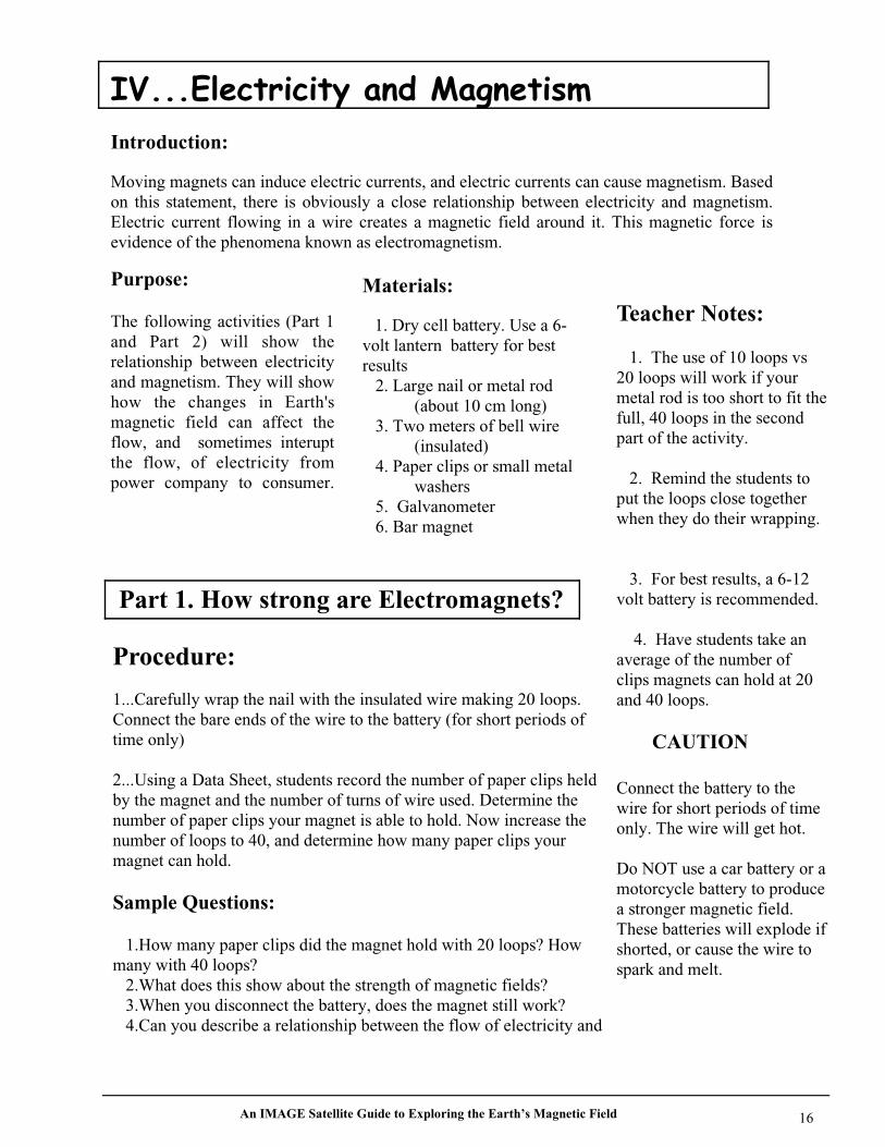
Moving magnets can induce electric currents, and electric currents can cause magnetism. Basedon this statement, there is obviously a close relationship between electricity and magnetism.Electric current flowing in a wire creates a magnetic field around it. This magnetic force isevidence of the phenomena known as electromagnetism.
Purpose:
The following activities (Part 1and Part 2) will show therelationship between electricityand magnetism. They will showhow the changes in Earth'smagnetic field can affect theflow, and sometimes interuptthe flow, of electricity frompower company to consumer.
Materials:
1. Dry cell battery. Use a 6-volt lantern battery for bestresults 2. Large nail or metal rod
(about 10 cm long) 3. Two meters of bell wire
(insulated) 4. Paper clips or small metal
washers 5. Galvanometer 6. Bar magnet
Procedure:
1...Carefully wrap the nail with the insulated wire making 20 loops.Connect the bare ends of the wire to the battery (for short periods oftime only)
2...Using a Data Sheet, students record the number of paper clips heldby the magnet and the number of turns of wire used. Determine thenumber of paper clips your magnet is able to hold. Now increase thenumber of loops to 40, and determine how many paper clips yourmagnet can hold.
Sample Questions:
1.How many paper clips did the magnet hold with 20 loops? Howmany with 40 loops? 2.What does this show about the strength of magnetic fields? 3.When you disconnect the battery, does the magnet still work? 4.Can you describe a relationship between the flow of electricity and
Teacher Notes:
1. The use of 10 loops vs20 loops will work if yourmetal rod is too short to fit thefull, 40 loops in the secondpart of the activity.
2. Remind the students toput the loops close togetherwhen they do their wrapping.
3. For best results, a 6-12volt battery is recommended.
4. Have students take anaverage of the number ofclips magnets can hold at 20and 40 loops.
CAUTION
Connect the battery to thewire for short periods of timeonly. The wire will get hot.
Do NOT use a car battery or amotorcycle battery to producea stronger magnetic field.These batteries will explode ifshorted, or cause the wire tospark and melt.
Part 1. How strong are Electromagnets?

An IMAGE Satellite Guide to Exploring the Earth’s Magnetic Field 17
Part 2. Making currents flow in a wire by magnetic induction.
In the last activity you were able to create a magnet using the flow of electricity through a wire. Thisis called an electromagnet. In this activity you will induce the flow of electricity in a wire using apermanent ‘bar’ magnet. The flow of electricity will be small so you will need to use thegalvanometer to measure the flow.
Note: A galvanometer is a piece of common high school laboratory equipment that can be boughtthrough school lab equipment suppliers. It is a meter that measures the current flow in a wire. Theyare also called ‘Am meters’ because they measure current flow in units called Amperes. These canalso be bought at electrical supply stores such as Radio Shack.
Using the same wire, make a coil big enough to allow the bar magnet to pass through. Hook the bareends of the wire to the galvanometer. Pass the bar magnet through the coils in a back and forthmotion, slowly then quickly. The movement of the needle on the galvanometer is caused by theinduced flow of electricity.
Teacher Notes:
1.A stronger bar magnet will yield better results. 2.Students may need to vary the number of coils to get good results, they may also need to alter thespeed at which they pass the bar magnet between the wire coils. 3. Students should observe that a current will only flow if the magnet is in motion.
Questions:
1.Does the speed at which you move the magnet through the wire coils have any affect on theneedle’s movement? What happens?
2.What do you think would happen if the power company was operating at 'full' capacity( such as during a heat wave or extreme cold spell) and a magnetic storm happened? Magnetic stormscause rapid changes in the magnetic field of Earth near ground level.
An IMAGE Satellite Guide to Exploring the Earth’s Magnetic Field 18
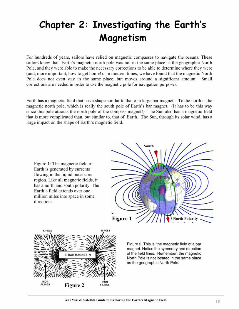
Figure 2: This is the magnetic field of a barmagnet. Notice the symmetry and directionof the field lines. Remember, the magnetic North Pole is not located in the same placeas the geographic North Pole.
Figure 1: The magnetic field ofEarth is generated by currentsflowing in the liquid outer coreregion. Like all magnetic fields, ithas a north and south polarity. TheEarth’s field extends over onemillion miles into space in somedirections.
For hundreds of years, sailors have relied on magnetic compasses to navigate the oceans. Thesesailors knew that Earth’s magnetic north pole was not in the same place as the geographic NorthPole, and they were able to make the necessary corrections to be able to determine where they were(and, more important, how to get home!). In modern times, we have found that the magnetic NorthPole does not even stay in the same place, but moves around a significant amount. Smallcorrections are needed in order to use the magnetic pole for navigation purposes.
Earth has a magnetic field that has a shape similar to that of a large bar magnet . To the north is themagnetic north pole, which is really the south pole of Earth’s bar magnet. (It has to be this waysince this pole attracts the north pole of the compass magnet!) The Sun also has a magnetic fieldthat is more complicated than, but similar to, that of Earth. The Sun, through its solar wind, has alarge impact on the shape of Earth’s magnetic field.
South
North PolarityFigure 1
Figure 2
An IMAGE Satellite Guide to Exploring the Earth’s Magnetic Field 19
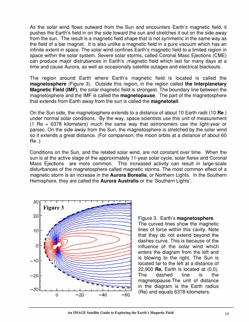
As the solar wind flows outward from the Sun and encounters Earth’s magnetic field, itpushes the Earth’s field in on the side toward the sun and stretches it out on the side awayfrom the sun. The result is a magnetic field shape that is not symmetric in the same way asthe field of a bar magnet. It is also unlike a magnetic field in a pure vacuum which has aninfinite extent in space. The solar wind confines Earth’s magnetic field to a limited region inspace within the solar system. Severe solar storms, called Coronal Mass Ejections (CME)can produce major distrubances in Earth’s ,magnetic field which last for many days at atime and cause Aurora, as well as occasionally satellite outages and electrical blackouts.
The region around Earth where Earth’s magnetic field is located is called themagnetosphere (Figure 3). Outside this region, in the region called the InterplanetaryMagnetic Field (IMF), the solar magnetic field is strongest. The boundary line between themagnetosphere and the IMF is called the magnetopause. The part of the magnetospherethat extends from Earth away from the sun is called the magnetotail.
On the Sun side, the magnetosphere extends to a distance of about 10 Earth radii (10 Re )under normal solar conditions. By the way, space scientists use this unit of measurement(1 Re = 6378 kilometers) much the same way that astronomers use the light-year orparsec. On the side away from the Sun, the magnetosphere is stretched by the solar windso it extends a great distance. (For comparison, the moon orbits at a distance of about 60Re .)
Conditions on the Sun, and the related solar wind, are not constant over time. When thesun is at the active stage of the approximately 11-year solar cycle, solar flares and CoronalMass Ejections are more common. This increased activity can result in large-scaledisturbances of the magnetosphere called magnetic storms. The most common effect of amagnetic storm is an increase in the Aurora Borealis, or Northern Lights. In the SouthernHemisphere, they are called the Aurora Australis or the ‘Southern Lights’.
Figure 3. Earth’s magnetosphere.The curved lines show the magneticlines of force within this cavity. Notethat they do not extend beyond thedashes curve. This is because of theinfluence of the solar wind whichenters the diagram from the left andis blowing to the right. The Sun islocated far to the left at a distance of22,900 Re. Earth is located at (0,0).The dashed line is themagnetopause.The unit of distancein the diagram is the Earth radius(Re) and equals 6378 kilometers.
Figure 3
An IMAGE Satellite Guide to Exploring the Earth’s Magnetic Field 20
Other effects are also observed and some of them are dangerous and can causeserious damage. These effects include:
1. Induced currents in power company transformers that can cause overloadconditions and damage equipment. It is thought that a magnetic stormthat resulted from a CME caused the blackout in the northeastern UnitedStates and eastern Canada in 1989.
2. Induced currents in pipelines can cause an increase in corrosion and canlead to leaks and breaks. The Alaskan oil pipeline was designed tominimize this effect.
3. Astronauts in space can be exposed to dangerous levels of chargedparticles. For this reason, astronauts working outside the space shuttlewould have to go inside if a solar storm were predicted or observed.
4. Heating of the atmosphere by solar particles causes the atmosphere toexpand. The increased friction causes satellites to lose energy anddescend into the atmosphere. This is the process that, over time, isthought to have caused the decay of the orbit of Skylab in the 1970’s.
5. Satellites in high orbits are subjected to energetic charged particles thatcan cause damage to electronic components. Failure of somecommunication satellites, which are in geosynchronous orbits, have beenattributed to the impact of severe solar storms.
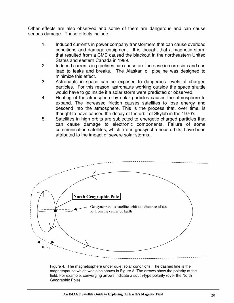
10 RE
Geosynchronous satellite orbit at a distance of 6.6RE from the center of Earth
Figure 4. The magnetosphere under quiet solar conditions. The dashed line is themagnetopause which was also shown in Figure 3. The arrows show the polarity of thefield. For example, converging arrows indicate a south-type polarity (over the NorthGeographic Pole)
North Geographic Pole
An IMAGE Satellite Guide to Exploring the Earth’s Magnetic Field 21
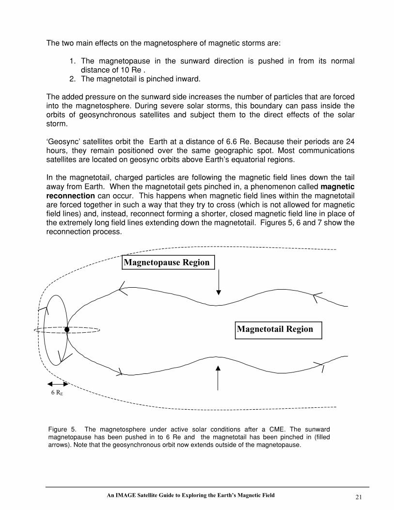
The two main effects on the magnetosphere of magnetic storms are:
1. The magnetopause in the sunward direction is pushed in from its normaldistance of 10 Re .
2. The magnetotail is pinched inward.
The added pressure on the sunward side increases the number of particles that are forcedinto the magnetosphere. During severe solar storms, this boundary can pass inside theorbits of geosynchronous satellites and subject them to the direct effects of the solarstorm.
‘Geosync’ satellites orbit the Earth at a distance of 6.6 Re. Because their periods are 24hours, they remain positioned over the same geographic spot. Most communicationssatellites are located on geosync orbits above Earth’s equatorial regions.
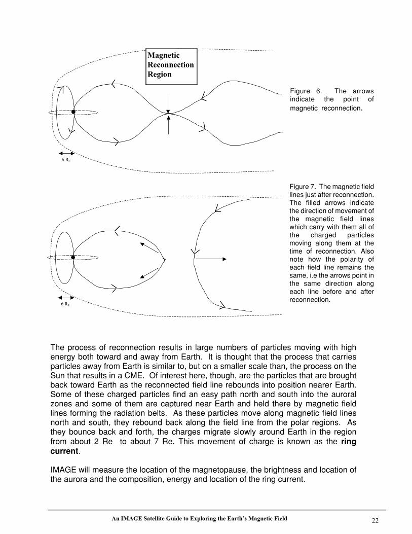
In the magnetotail, charged particles are following the magnetic field lines down the tailaway from Earth. When the magnetotail gets pinched in, a phenomenon called magneticreconnection can occur. This happens when magnetic field lines within the magnetotailare forced together in such a way that they try to cross (which is not allowed for magneticfield lines) and, instead, reconnect forming a shorter, closed magnetic field line in place ofthe extremely long field lines extending down the magnetotail. Figures 5, 6 and 7 show thereconnection process.
Figure 5. The magnetosphere under active solar conditions after a CME. The sunwardmagnetopause has been pushed in to 6 Re and the magnetotail has been pinched in (filledarrows). Note that the geosynchronous orbit now extends outside of the magnetopause.
6 RE
Magnetotail Region
Magnetopause Region
An IMAGE Satellite Guide to Exploring the Earth’s Magnetic Field 22
The process of reconnection results in large numbers of particles moving with highenergy both toward and away from Earth. It is thought that the process that carriesparticles away from Earth is similar to, but on a smaller scale than, the process on theSun that results in a CME. Of interest here, though, are the particles that are broughtback toward Earth as the reconnected field line rebounds into position nearer Earth.Some of these charged particles find an easy path north and south into the auroralzones and some of them are captured near Earth and held there by magnetic fieldlines forming the radiation belts. As these particles move along magnetic field linesnorth and south, they rebound back along the field line from the polar regions. Asthey bounce back and forth, the charges migrate slowly around Earth in the regionfrom about 2 Re to about 7 Re. This movement of charge is known as the ringcurrent.
IMAGE will measure the location of the magnetopause, the brightness and location ofthe aurora and the composition, energy and location of the ring current.
Figure 6. The arrowsindicate the point ofmagnetic reconnection.
6 RE
6 RE
Figure 7. The magnetic fieldlines just after reconnection.The filled arrows indicatethe direction of movement ofthe magnetic field lineswhich carry with them all ofthe charged particlesmoving along them at thetime of reconnection. Alsonote how the polarity ofeach field line remains thesame, i.e the arrows point inthe same direction alongeach line before and afterreconnection.
MagneticReconnectionRegion
An IMAGE Satellite Guide to Exploring the Earth’s Magnetic Field 23
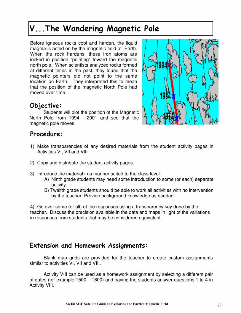
Before igneous rocks cool and harden, the liquidmagma is acted on by the magnetic field of Earth.When the rock hardens, these iron atoms arelocked in position "pointing" toward the magneticnorth pole. When scientists analyzed rocks formedat different times in the past, they found that themagnetic pointers did not point to the samelocation on Earth. They interpreted this to meanthat the position of the magnetic North Pole hadmoved over time.
Students will plot the position of the MagneticNorth Pole from 1994 - 2001 and see that themagnetic pole moves.
1) Make transparencies of any desired materials from the student activity pages inActivities VI, VII and VIII..
2) Copy and distribute the student activity pages.
3) Introduce the material in a manner suited to the class level:A) Ninth grade students may need some introduction to some (or each) separate
activity.B) Twelfth grade students should be able to work all activities with no intervention
by the teacher. Provide background knowledge as needed.
4) Go over some (or all) of the responses using a transparency key done by theteacher. Discuss the precision available in the data and maps in light of the variationsin responses from students that may be considered equivalent.
Blank map grids are provided for the teacher to create custom assignmentssimilar to activities VI, VII and VIII.
Activity VIII can be used as a homework assignment by selecting a different pairof dates (for example 1500 – 1600) and having the students answer questions 1 to 4 inActivity VIII.
An IMAGE Satellite Guide to Exploring the Earth’s Magnetic Field 24
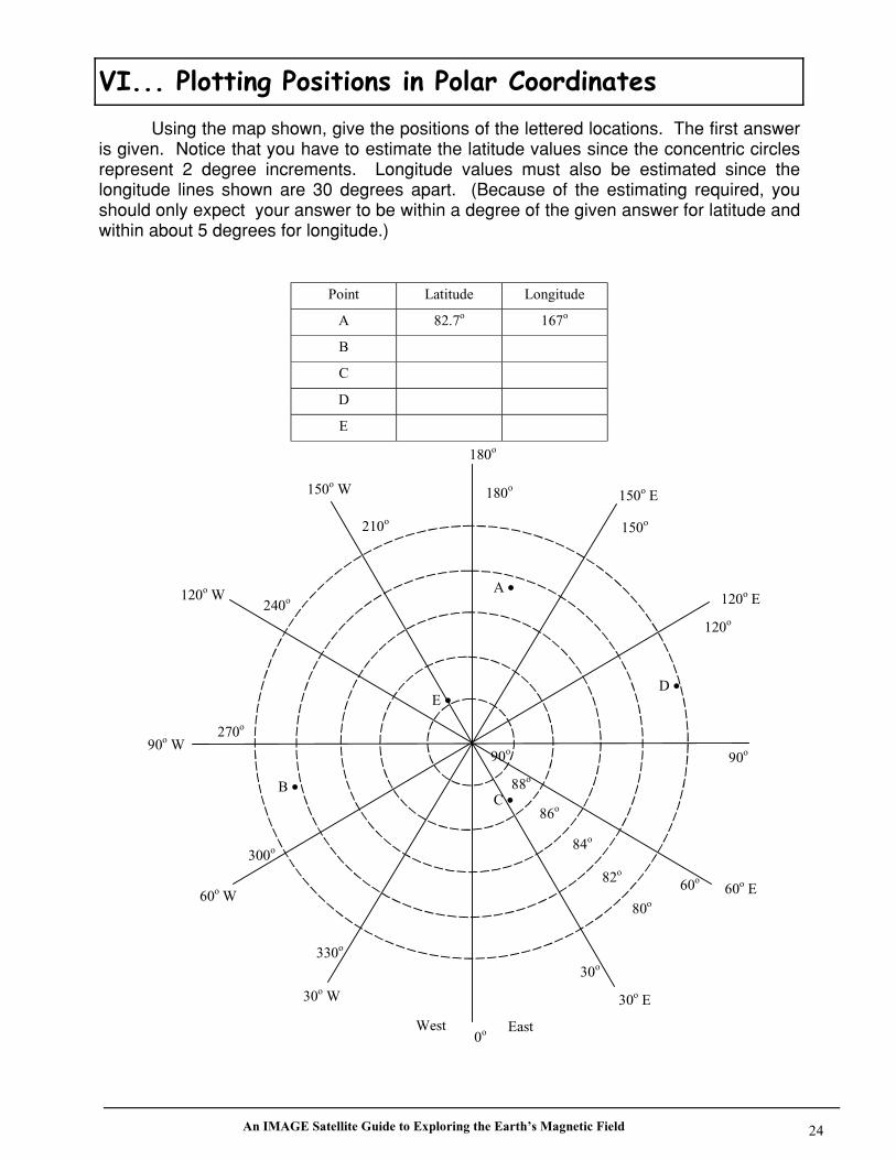
Using the map shown, give the positions of the lettered locations. The first answeris given. Notice that you have to estimate the latitude values since the concentric circlesrepresent 2 degree increments. Longitude values must also be estimated since thelongitude lines shown are 30 degrees apart. (Because of the estimating required, youshould only expect your answer to be within a degree of the given answer for latitude andwithin about 5 degrees for longitude.)
Point Latitude Longitude
A 82.7o 167o
B
C
D
E
West East0o
30o
60o
120o E
150o E
60o E
30o E
180o
180o
150o
120o
90o
30o W
60o W
90o W
120o W
150o W
210o
240o
270o
300o
330o
90o
88o
86o
84o
82o
80o
A •
B •
D •
C •
E •
An IMAGE Satellite Guide to Exploring the Earth’s Magnetic Field 25
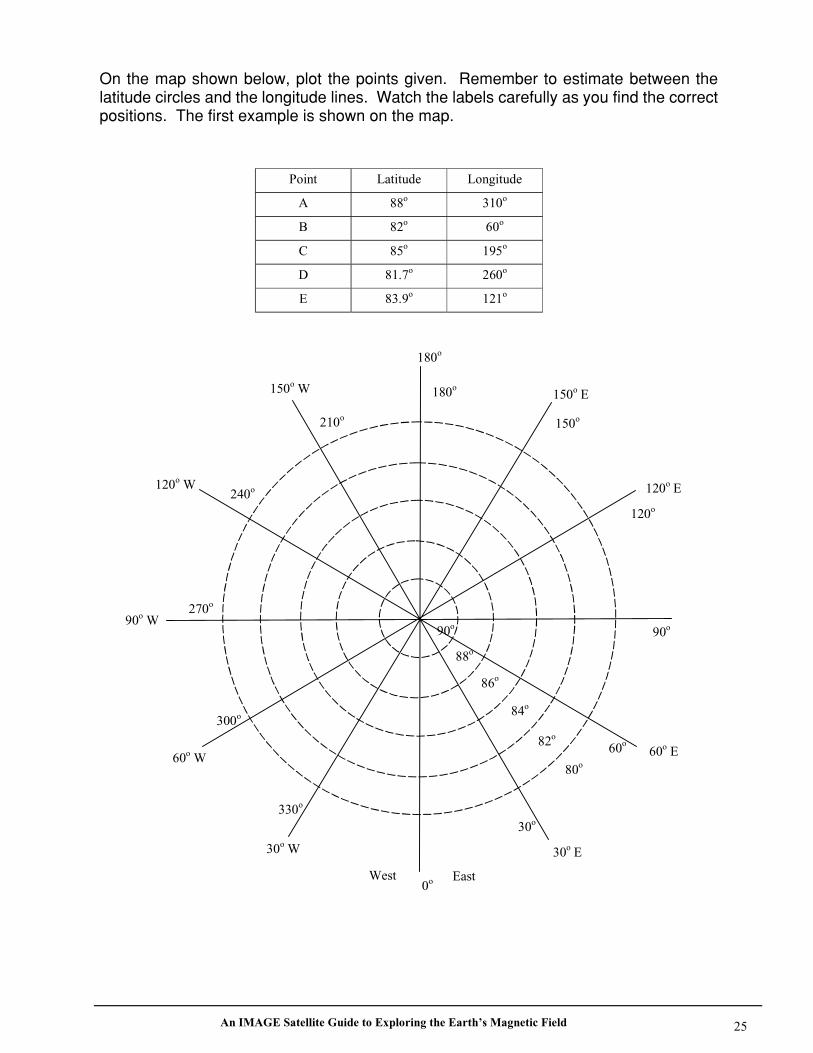
On the map shown below, plot the points given. Remember to estimate between thelatitude circles and the longitude lines. Watch the labels carefully as you find the correctpositions. The first example is shown on the map.
Point Latitude Longitude
A 88o 310o
B 82o 60o
C 85o 195o
D 81.7o 260o
E 83.9o 121o
West East0o
30o
60o
120o E
150o E
60o E
30o E
180o
180o
150o
120o
90o
30o W
60o W
90o W
120o W
150o W
210o
240o
270o
300o
330o
90o
88o
86o
84o
82o
80o
An IMAGE Satellite Guide to Exploring the Earth’s Magnetic Field 26
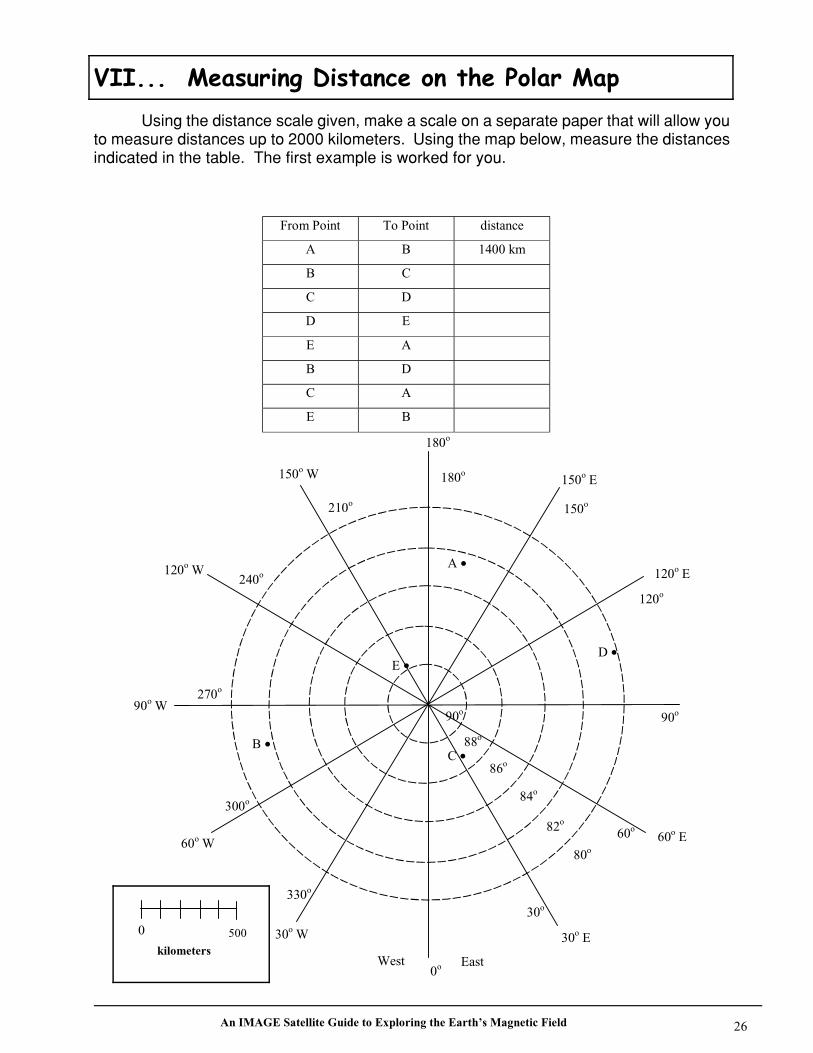
Using the distance scale given, make a scale on a separate paper that will allow youto measure distances up to 2000 kilometers. Using the map below, measure the distancesindicated in the table. The first example is worked for you.
From Point To Point distance
A B 1400 km
B C
C D
D E
E A
B D
C A
E B
West East0o
30o
60o
120o E
150o E
60o E
30o E
180o
180o
150o
120o
90o
30o W
60o W
90o W
120o W
150o W
210o
240o
270o
300o
330o
90o
88o
86o
84o
82o
80o
A •
B •
D •
C •
E •
0 500 kilometerskilometers
500
An IMAGE Satellite Guide to Exploring the Earth’s Magnetic Field 27
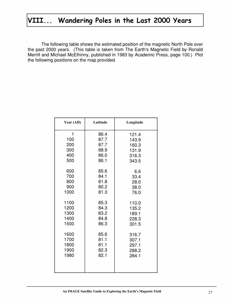
The following table shows the estimated position of the magnetic North Pole overthe past 2000 years. (This table is taken from The Earth's Magnetic Field by RonaldMerrill and Michael McElhinny, published in 1983 by Academic Press, page 100.) Plotthe following positions on the map provided.
1100200300400500
600700800900
1000
11001200130014001500
16001700180019001980
86.487.787.788.986.086.1
85.684.181.880.281.3
85.384.383.284.886.3
85.681.181.182.382.1
121.4143.9160.3131.9316.3343.5
6.633.428.038.076.0
110.0135.2189.1228.3301.5
316.7307.1297.1288.2284.1
Year (AD) Latitude Longitude
An IMAGE Satellite Guide to Exploring the Earth’s Magnetic Field 28
West East0o
30o
60o
120o E
150o E
60o E
30o E
180o
180o
150o
120o
90o
30o W
60o W
90o W
120o W
150o W
210o
240o
270o
300o
330o
90o
88o
86o
84o
82o
80o
0 500 kilometers
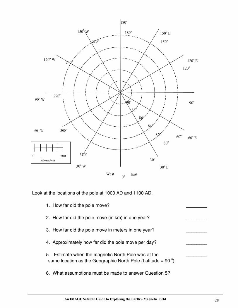
Look at the locations of the pole at 1000 AD and 1100 AD.
1. How far did the pole move? ________
2. How far did the pole move (in km) in one year? ________
3. How far did the pole move in meters in one year? ________
4. Approximately how far did the pole move per day? ________
5. Estimate when the magnetic North Pole was at the ________ same location as the Geographic North Pole (Latitude = 90 o).
6. What assumptions must be made to answer Question 5?
300o60o W
0 500 kilometers
An IMAGE Satellite Guide to Exploring the Earth’s Magnetic Field 29
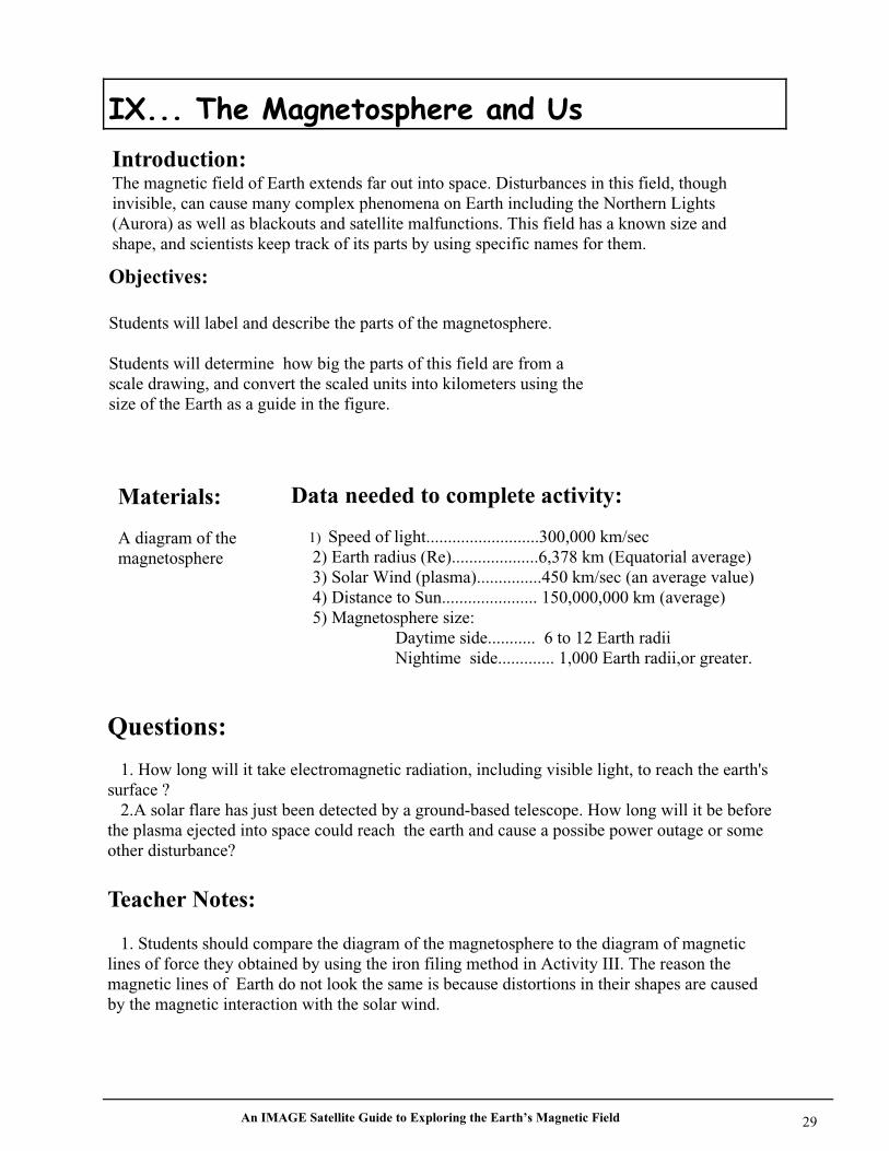
Materials:
A diagram of themagnetosphere
Questions:
1. How long will it take electromagnetic radiation, including visible light, to reach the earth'ssurface ? 2.A solar flare has just been detected by a ground-based telescope. How long will it be beforethe plasma ejected into space could reach the earth and cause a possibe power outage or someother disturbance?
Data needed to complete activity:
1) Speed of light..........................300,000 km/sec 2) Earth radius (Re)....................6,378 km (Equatorial average) 3) Solar Wind (plasma)...............450 km/sec (an average value) 4) Distance to Sun...................... 150,000,000 km (average) 5) Magnetosphere size:
Daytime side........... 6 to 12 Earth radii Nightime side............. 1,000 Earth radii,or greater.
Teacher Notes:
1. Students should compare the diagram of the magnetosphere to the diagram of magneticlines of force they obtained by using the iron filing method in Activity III. The reason themagnetic lines of Earth do not look the same is because distortions in their shapes are causedby the magnetic interaction with the solar wind.
Introduction:The magnetic field of Earth extends far out into space. Disturbances in this field, thoughinvisible, can cause many complex phenomena on Earth including the Northern Lights(Aurora) as well as blackouts and satellite malfunctions. This field has a known size andshape, and scientists keep track of its parts by using specific names for them.
Objectives:
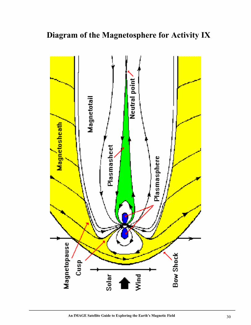
Students will label and describe the parts of the magnetosphere.
Students will determine how big the parts of this field are from ascale drawing, and convert the scaled units into kilometers using thesize of the Earth as a guide in the figure.
An IMAGE Satellite Guide to Exploring the Earth’s Magnetic Field 30
Diagram of the Magnetosphere for Activity IX
An IMAGE Satellite Guide to Exploring the Earth’s Magnetic Field 31
Anyone can tell you that a compass points 'north' because Earth has a magnetic field, but until theadvent of the Space Age, no one really understood what this field really looked like or was capable ofdoing. Since Gilbert proposed in the 17th century that Earth was a giant magnet, scientists havewondered just how this field is shaped, and how it has changed with time. The geomagnetic fieldwhich gives us our familiar compass bearings, also extends thousands of kilometers out into space in aregion called the magnetosphere. On the Sun-side, it forms a protective boundary called the bowshock.
Stretching millions of miles in the opposite direction behind Earth is the magnetotail. The solar windblows upon the magnetosphere and gives it a wind-swept shape, but when solar storms and solar windstreams reach Earth, the magnetosphere reacts violently. On the side nearest the impact, themagnetosphere compresses like a balloon, leaving communications satellites exposed. On the oppositeside, it is stretched out, past the orbit of the Moon, or Mars and even Jupiter! The geomagnetic field isremarkably stiff, and so most of the solar wind is deflected or just slips by without notice. But some ofthe matter leaks in and takes up residence in donut-shaped clouds of trapped particles, or can penetrateto the atmosphere to produce the Northern Lights.
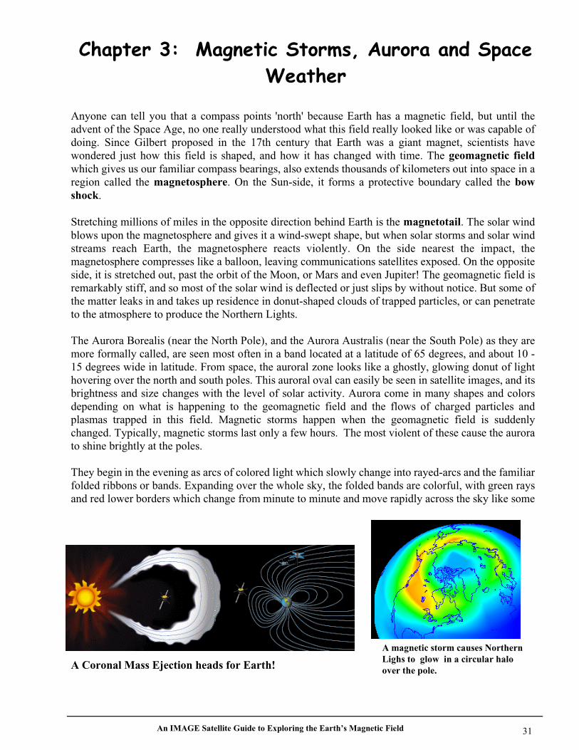
The Aurora Borealis (near the North Pole), and the Aurora Australis (near the South Pole) as they aremore formally called, are seen most often in a band located at a latitude of 65 degrees, and about 10 -15 degrees wide in latitude. From space, the auroral zone looks like a ghostly, glowing donut of lighthovering over the north and south poles. This auroral oval can easily be seen in satellite images, and itsbrightness and size changes with the level of solar activity. Aurora come in many shapes and colorsdepending on what is happening to the geomagnetic field and the flows of charged particles andplasmas trapped in this field. Magnetic storms happen when the geomagnetic field is suddenlychanged. Typically, magnetic storms last only a few hours. The most violent of these cause the aurorato shine brightly at the poles.
They begin in the evening as arcs of colored light which slowly change into rayed-arcs and the familiarfolded ribbons or bands. Expanding over the whole sky, the folded bands are colorful, with green raysand red lower borders which change from minute to minute and move rapidly across the sky like some
A Coronal Mass Ejection heads for Earth!
A magnetic storm causes NorthernLighs to glow in a circular haloover the pole.

An IMAGE Satellite Guide to Exploring the Earth’s Magnetic Field 32
Introduction
Solar storms can affect Earth's magnetic field causing small changes in its direction at thesurface which are called 'magnetic storms'. A magnetometer operates like a sensitive compassand senses these slight changes. The soda bottle magnetometer is a simple device that can bebuilt for under $5.00 which will let students monitor these changes in the magnetic field thatoccur inside the classroom. When magnetic storms occur, you will see the direction that themagnet points change by several degrees within a few hours, and then return to its normalorientation pointing towards the magnetic north pole.
Objective:
The students will create amagnetometer to monitor changes inEarth's magnetic field for signs of
Teacher Notes:
1) Do not use common ‘refrigerator’ plastic/rubbermagnets because they are not properly polarized.Use only a true N-S bar magnet.
2) Superglue is useful for mounting the magnet onthe card in a hurry, but be careful not to glue thecard to the table underneath as the glue has a habitof leaking through the paper if too much is used.
3) In the January 1999 issue of ScientificAmerican, there is a design for a magnetometerthat uses a torsion wire and laser pointerdeveloped by amateur scientist Roger Baker. Youcan visit the Scientific American pages online toget more information on these other designs.
Materials
One clean 2 liter soda bottle 2 pounds of sand 2 feet of sewing thread A 1 inch piece of soda straw Super glue (be careful!) 2 inch clear packing tape A meter stick A 3x5 index card
A small bar magnetGet this from the Magnet Source. They offer aRed Ceramic Bar Magnet with 'N' and 'S'marked. It is 1.5" long. $0.48 each. CatalogNumber DMCPB. Call 1-800-525-3536 or 1-888-293-9190 for ordering and details.
A mirrored dress sequin, or small craftmirror. Darice, Inc. 1/2-inch round mirror, item No.1613-41, $0.99 for 10. Order from Darice Inc1-800-321-1494. mail: 13000 Darice Parkway,Park 82, Strongsville, Ohio, 44136-6699.Available at Crafts Stores under trademark'Darice Craft Designer'
Light Sources:
A goose neck high-intensity lamp with a clearbulb.
Alternative light source:
A laser pointer. You will need a test tube ringstand and a clamp to hold it securely.
Safety Concern: To avoid eye damage,students muct be told NOT to look directlyinto laser beam.
An IMAGE Satellite Guide to Exploring the Earth’s Magnetic Field 33
Procedure
1. Clean the soda bottle thoroughly and remove labeling. 2. Slice the bottle 1/3 of the way down from the top of the bottle. 3. Pierce a small hole in the center of the cap. 4. Fill the bottom section with sand. About 2-3 cups to serve as a suitable weight. 5. Cut the index card so that it fits inside the bottle (See Figure 1). 6. Glue the magnet to the center of the top edge of the card. 7. Glue a 1 inch piece of soda straw to the top of the magnet. 8. Glue the mirror spot to the front of the magnet. 9. Thread the thread through the soda straw and tie it into a small triangle with 2 inch sides. 10. Tie a 6 inch thread to the top of the triangle in #9 and thread it through the hole in the
cap. 11. Put the bottle top and bottom together so that the 'sensor card' is free to swing with the
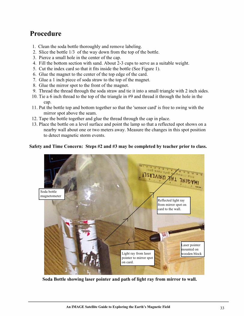
mirror spot above the seam. 12. Tape the bottle together and glue the thread through the cap in place. 13. Place the bottle on a level surface and point the lamp so that a reflected spot shows on a
nearby wall about one or two meters away. Measure the changes in this spot position to detect magnetic storm events.
Safety and Time Concern: Steps #2 and #3 may be completed by teacher prior to class.
Light ray from laserpointer to mirror spoton card.
Reflected light rayfrom mirror spot oncard to the wall.
Laser pointermounted onwooden block
Soda bottlemagnetometer
Soda Bottle showing laser pointer and path of light ray from mirror to wall.
An IMAGE Satellite Guide to Exploring the Earth’s Magnetic Field 34
Tips
It is important that when you adjust the location of the sensor card inside the bottle that itsedges do not touch the inside of the bottle. Be sure that the mirror spot is above the seam andthe taping region of this seam, so that it is unobstructed and free to spin around the suspensionthread.
The magnetometer must be placed in an undisturbed location of the classroom where you canalso set up the high intensity lamp so that a reflected spot can be cast on a wall within 1 meter ofthe center of the bottle. This allows a 1 centimeter change in the light spot position to equal 1/4degree in angular shift of the magnetic North Pole. At half this distance, 1 centimeter will equal1/2 a degree. Because magnetic storms produce shifts up to 5 or more degrees for somegeographic locations, you will not need to measure angular shifts smaller than 1/4 degrees.Typically, these magnetic storms last a few hours or less.
To begin a measuring session which could last for several months, note the location of the spoton the wall by a small pencil mark. Measure the magnetic activity from day to day bymeasuring the distance between this reference spot and the current spot whose position you willmark, and note the date and the time of day. Measure the distance to the reference mark and thenewspot in centimeters. Convert this into degrees of deflection for a 1 meter distance by multiplyingby 1/4 degrees for each centimeter of displacement.
You can check that this magnetometer is working by comparing the card's pointing directionwith an ordinary compass needle, which should point parallel to the magnet in the soda bottle.You can also note this direction by marking the position of the light spot on the wall.
If you must move the soda bottle, you will have to note a new reference mark for the light spotand the resume measuring the new deflections from the new reference mark as before.
Most of the time there will be few detectable changes in the spot's location, so you will have toexercise some patience. However, as we begin to move away from sunspot maximum betweenafter 2001, there should still be several good storms every few months. Large magnetic stormsare accompanied by major aurora displays, so you may want to use your magnetometer in theday time to predict if you will see a good aurora display after sunset. Note: Professionalphotographers use a similar device to get ready for photographing aurora in Alaska andCanada.
This magnetometer is sensitive enough to detect cars moving on a street outside your room.With a 1-meter distance between the mirror and the screen, a car moving 30-50 feet awayproduces a sudden deviation by up to 1 inch from its refeence position. The oscillationfrequency of the magnet on the card is about 4 seconds and after a car passes, the amplitude ofthe spot motion will decrease for 5-10 cycles before returning to its rest position. You can evendetermine the direction of the car's motion by seeing if the spot initially moves east or west!Also, by moving a large mass of metal...say 30 lbs of iron nails...at distances of 1 meter to 5meters from the magnet, you can measure the amount of deflection you get on the spot, and byplotting this, you may attempt to recover the 'inverse-cube' law for magnetism. This would bean advanced project for middle-school students, but they would see that magnetism falls-offwith distance, which is the main point of the plotting exercise.

An IMAGE Satellite Guide to Exploring the Earth’s Magnetic Field 35
The following information is a step-by-step guide for setting up the magnetometer at home, andmaking and recording the measurements.
1) During each of the participating school periods, ask for a volunteer from each of the groupsto bring the magnetometer home.
2) Have the student pick up the magnetometer after school to minimize damaging the system.
3) Once the magnetometer arrives at home, the student will need to find a room where theinstrument will remain undisturbed for the next three days. The student will have to inspect theinstrument for damage during transport from school, and make the necessary repairs so that thesensor card hangs freely inside the bottle and does not scrape the inside of the bottle as it moves.
4) Obtain a high-intensity lamp, or a desk lamp with a CLEAR bulb. Do not use a bulb with afrosted lamp because you will not be able to see a glint off of the mirror with such a bulb. Theglint/spot you are looking for is actually the image of the filament of the lamp.
5) With the magnetometer positioned 1 meter (39 inches) from a wall on a table, position thelamp so that the center of the bulb shines at a 45-degree angle to the mirror. Search for a glint orspot of light from the mirror on the wall. Make sure the table is stable and not rickety becauseany vibration of the table will make reading the spot location very difficult. You may also haveto relocate the magnetometer several times until you find a convenient location in your housewhere the spot falls on a wall 1-meter from the magnetometer.
6) Once again, make certain that the sensor card is free to rotate horizontally inside the bottleafter you have finished this set-up process.
7) On an 8 1/2 x 11 inch piece of white paper, draw a horizontal line along the center of the longdirection of the paper so that you have a line that divides the paper into two parts 4 1/4 x 11inches in size.
8) With a centimeter ruler, draw tic marks every 1 centimeter on this line starting from the left-hand end of the line. Label the first mark on the left end '0', and then below the line, label theodd-numbered marks with their centimeter numbers. '0, 1, 3, 5, ...' If you label every tic mark,the scale will be too cluttered to easily read from a 1-meter distance.
9) With the lamp turned on and properly positioned, find the spot on the wall, and position thepaper with the centimeter scale, horizontally on the wall. Before securing to the wall, make surethat as the spot moves from side to side on the wall, that it travels along the centimeter scale in aparallel fashion. It is convenient to have the spot moving in a parallel line offset about 1 inchabove the centimeter scale.
10) At the start of your 3-day observing sequence, you will need to shift the
Setting up to take data:
An IMAGE Satellite Guide to Exploring the Earth’s Magnetic Field 36
Making the measurements:
1) For three days of recording, you will be able to fit Day 1 and Day 2 on the front side of asheet of ruled paper, and Day 3 on the back side. For each day, leave a blank for the date,followed by 4 columns which you will label from left to right 'Time' 'Position' 'Amplitude''Comments'.
2) In the 'Time' column, write down the following times in a vertical list:
5:00 PM 5:30 6:00 6:30 7:00 7:30 8:00 8:30 9:00 9:30 10:00
3) The first reading you will make on the first day will always be '15.0' because that is whereyou set-up the scale on the spot in Step 10 in the instructions above. For the subsequentmeasurements, you will record the actual spot location on your scale. Do NOT reposition thespot every day. You just need to do this one time at the start of your 2, 3, 5 ...day measurementseries.
4) When making a measurement, turn on and off the lamp from the wall plug only. This willavoid accidental vibration or lamp motion if you were to try using the switch on the lamp.You want to avoid disturbing the lamp, magnetometer and centimeter scale during the three-day session.
5) If you know, for a fact, that the set up was disturbed, recenter the centimeter scale on thecurrent spot position at the '15 centimeter' point. Make a note that you did this on the data tableat the appropriate time, you can then resume taking normal data at the next assigned time inthe data table. Warning, do not assume that just because a big change in the readingsoccurred, that the instrument was disturbed. You could have detected a magnetic storm!! Onlyrecenter the scale if you physically saw the instrument disturbed, or someone told you thatthey accidentally touched it.
6) It is important that you make your measurements within 5 minutes of the times listed in thedata table. If you are unable to do this for any entry, leave it blank and do not attempt to'fudge' or estimate what the value could have been. Chances are very good that anotherstudent in the network will have made the missing' measurement.
An IMAGE Satellite Guide to Exploring the Earth’s Magnetic Field 37
7) The spot on the wall will probably be irregular in shape. Make yourself familiar with whatthe spot looks like as it moves, and find a portion of the spot that has a good, sharp edge, orsome other easily recognized feature. You can also estimate by eye where the center of the spotis if the spot has a simple...round..shape. Try to make all of your measurements in a consistentway each time, and to estimate the spot location to the nearest 0.5 centimeter. Record thisnumber in Column 2 in your data sheet.
8) You may notice several 'behaviors' of the spot. It will either just sit at one location, or itmay oscillate from side to side. At a 1-meter distance from the magnetometer, if the spotswings back and forth horizontally by an amount LESS than 0.5 centimeters, consider the spot'Stationary' and write 'S' in Column 3 after your measurement. If it is obvious that the spot isoscillating back and forth, write 'O' in Column 3 and in Column 4 write down the range of theswing in centimeters along the scale. Example, if it moves from 13.0 centimeters to 17.0centimeters, write the average position of '15.0' centimeters in Column 2, and then write '13.0- 17.0' in Column 4.
9) The last thing you would want to note in your data log is local weather conditions IF there isa lightning storm going on. Note the time that the lightning began and ended as a 'Note' on thedata page, but don't write this in the data table itself. You also want to mention if the streetoutside your house is busy with traffic or not. An estimate of how often a car passeswould be good to note.
10) When your assigned time is finished, bring the data table and magnetometer back to school.
3-15-99
11:05 9.5 cm11:35 8.5 cm13:25 9.0 cm14:00 9.0 cm14:20 9.0 cm15:25 9.0 cm16:00 8.0 cm17:00 7.5 cm17:25 8.0 cm
3-17-99
9:45 6.5 cm10:40 6.5 cm11:05 6.0 cm11:40 4.0 cm12:15 4.5 cm13:00 6.0 cm13:30 7.0 cm15:35 1.5 cm16:10 2.5 cm
3-16-99
9:25 8.0 cm10:20 6.5 cm13:20 5.0 cm14:25 4.5 cm15:00 4.5 cm15:20 4.0 cm16:10 4.5 cm16:50 4.5 cm
Sample Data. Case 1.
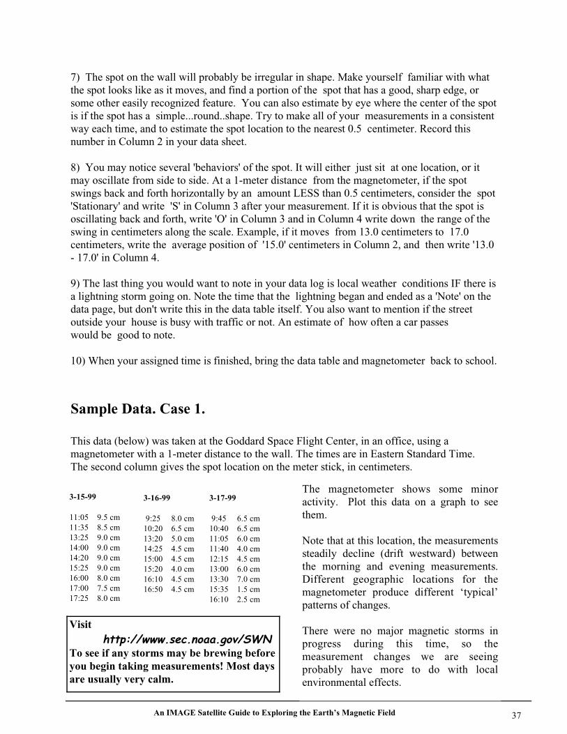
This data (below) was taken at the Goddard Space Flight Center, in an office, using amagnetometer with a 1-meter distance to the wall. The times are in Eastern Standard Time.The second column gives the spot location on the meter stick, in centimeters.
The magnetometer shows some minoractivity. Plot this data on a graph to seethem.
Note that at this location, the measurementssteadily decline (drift westward) betweenthe morning and evening measurements.Different geographic locations for themagnetometer produce different ‘typical’patterns of changes.
There were no major magnetic storms inprogress during this time, so themeasurement changes we are seeingprobably have more to do with localenvironmental effects.
Visit
To see if any storms may be brewing beforeyou begin taking measurements! Most daysare usually very calm.
An IMAGE Satellite Guide to Exploring the Earth’s Magnetic Field 38
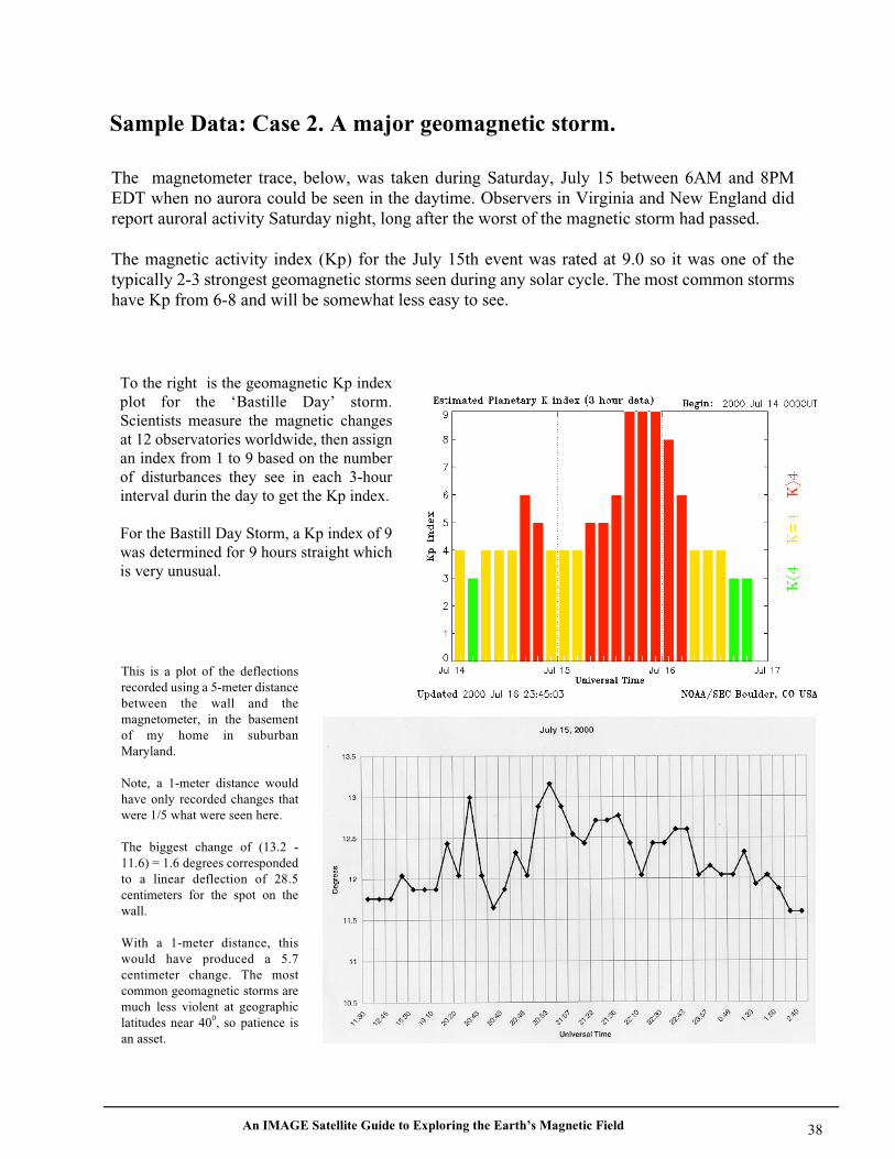
The magnetometer trace, below, was taken during Saturday, July 15 between 6AM and 8PMEDT when no aurora could be seen in the daytime. Observers in Virginia and New England didreport auroral activity Saturday night, long after the worst of the magnetic storm had passed.
The magnetic activity index (Kp) for the July 15th event was rated at 9.0 so it was one of thetypically 2-3 strongest geomagnetic storms seen during any solar cycle. The most common stormshave Kp from 6-8 and will be somewhat less easy to see.
Sample Data: Case 2. A major geomagnetic storm.
To the right is the geomagnetic Kp indexplot for the ‘Bastille Day’ storm.Scientists measure the magnetic changesat 12 observatories worldwide, then assignan index from 1 to 9 based on the numberof disturbances they see in each 3-hourinterval durin the day to get the Kp index.
For the Bastill Day Storm, a Kp index of 9was determined for 9 hours straight whichis very unusual.
This is a plot of the deflectionsrecorded using a 5-meter distancebetween the wall and themagnetometer, in the basementof my home in suburbanMaryland.
Note, a 1-meter distance wouldhave only recorded changes thatwere 1/5 what were seen here.
The biggest change of (13.2 -11.6) = 1.6 degrees correspondedto a linear deflection of 28.5centimeters for the spot on thewall.
With a 1-meter distance, thiswould have produced a 5.7centimeter change. The mostcommon geomagnetic storms aremuch less violent at geographiclatitudes near 400, so patience isan asset.
An IMAGE Satellite Guide to Exploring the Earth’s Magnetic Field 39
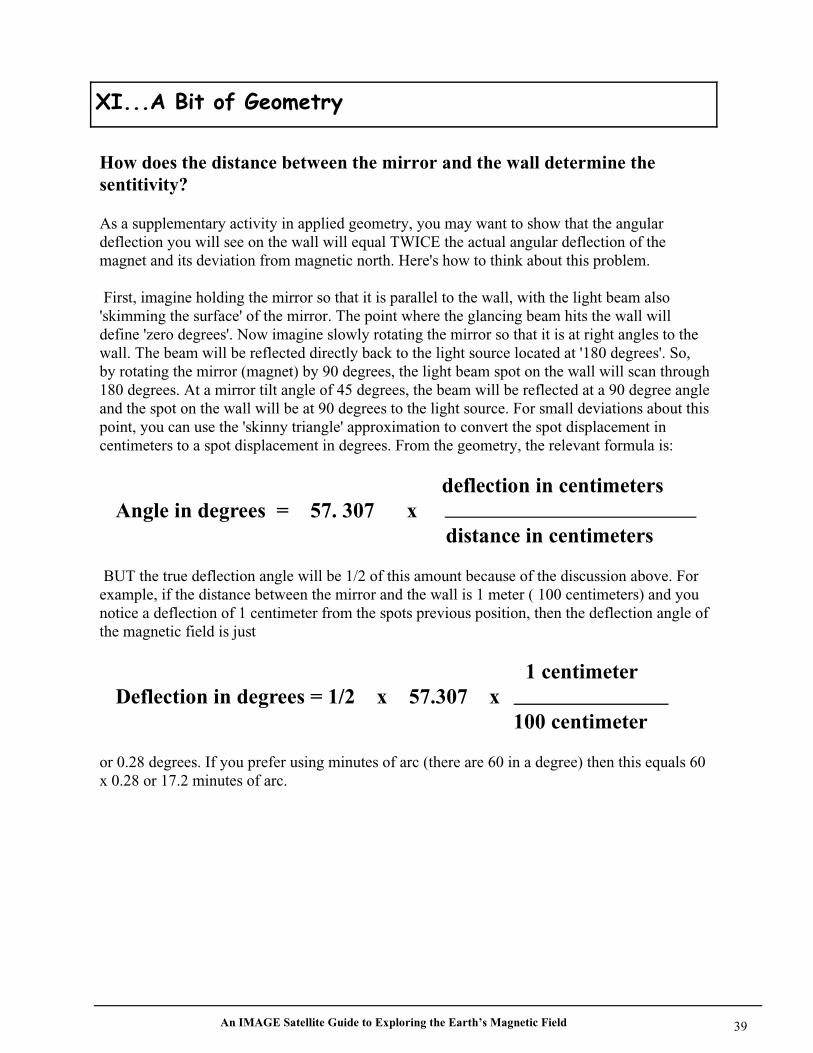
How does the distance between the mirror and the wall determine thesentitivity?
As a supplementary activity in applied geometry, you may want to show that the angulardeflection you will see on the wall will equal TWICE the actual angular deflection of themagnet and its deviation from magnetic north. Here's how to think about this problem.
First, imagine holding the mirror so that it is parallel to the wall, with the light beam also'skimming the surface' of the mirror. The point where the glancing beam hits the wall willdefine 'zero degrees'. Now imagine slowly rotating the mirror so that it is at right angles to thewall. The beam will be reflected directly back to the light source located at '180 degrees'. So,by rotating the mirror (magnet) by 90 degrees, the light beam spot on the wall will scan through180 degrees. At a mirror tilt angle of 45 degrees, the beam will be reflected at a 90 degree angleand the spot on the wall will be at 90 degrees to the light source. For small deviations about thispoint, you can use the 'skinny triangle' approximation to convert the spot displacement incentimeters to a spot displacement in degrees. From the geometry, the relevant formula is:
deflection in centimeters Angle in degrees = 57. 307 x distance in centimeters
BUT the true deflection angle will be 1/2 of this amount because of the discussion above. Forexample, if the distance between the mirror and the wall is 1 meter ( 100 centimeters) and younotice a deflection of 1 centimeter from the spots previous position, then the deflection angle ofthe magnetic field is just
1 centimeter Deflection in degrees = 1/2 x 57.307 x 100 centimeter
or 0.28 degrees. If you prefer using minutes of arc (there are 60 in a degree) then this equals 60x 0.28 or 17.2 minutes of arc.
An IMAGE Satellite Guide to Exploring the Earth’s Magnetic Field 40
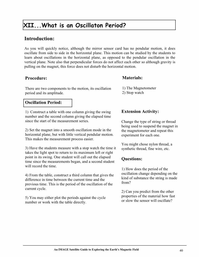
Introduction:
As you will quickly notice, although the mirror sensor card has no pendular motion, it doesoscillate from side to side in the horizontal plane. This motion can be studied by the students tolearn about oscillations in the horizontal plane, as opposed to the pendular oscillation in thevertical plane. Note also that perpendicular forces do not affect each other so although gravity ispulling on the magnet, this force does not disturb the horizontal motion.
Materials:
1) The Magnetometer2) Stop watch
Procedure:
There are two components to the motion, its oscillationperiod and its amplitude.
Oscillation Period:
1) Construct a table with one column giving the swingnumber and the second column giving the elapsed timesince the start of the measurement series.
2) Set the magnet into a smooth oscillation mode in thehorizontal plane, but with little vertical pendular motion.This makes the measurement process easier.
3) Have the students measure with a stop watch the time ittakes the light spot to return to its maximum left or rightpoint in its swing. One student will call out the elapsedtime since the measurements began, and a second studentwill record the time.
4) From the table, construct a third column that gives thedifference in time between the current time and theprevious time. This is the period of the oscillation of thecurrent cycle.
5) You may either plot the periods against the cyclenumber or work with the table directly.
Extension Activity:
Change the type of string or threadbeing used to suspend the magnet inthe magnetometer and repeat thisexperiment for each one.
You might chose nylon thread, asynthetic thread, fine wire, etc.
Questions:
1) How does the period of theoscillation change depending on thekind of substance the string is madefrom?
2) Can you predict from the otherproperties of the material how fastor slow the sensor will oscillate?
An IMAGE Satellite Guide to Exploring the Earth’s Magnetic Field 41
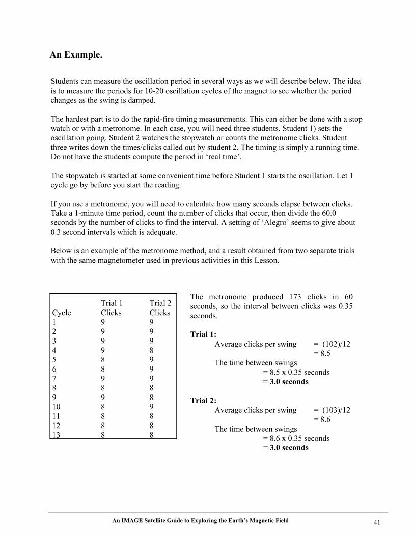
An Example.
Students can measure the oscillation period in several ways as we will describe below. The ideais to measure the periods for 10-20 oscillation cycles of the magnet to see whether the periodchanges as the swing is damped.
The hardest part is to do the rapid-fire timing measurements. This can either be done with a stopwatch or with a metronome. In each case, you will need three students. Student 1) sets theoscillation going. Student 2 watches the stopwatch or counts the metronome clicks. Studentthree writes down the times/clicks called out by student 2. The timing is simply a running time.Do not have the students compute the period in ‘real time’.
The stopwatch is started at some convenient time before Student 1 starts the oscillation. Let 1cycle go by before you start the reading.
If you use a metronome, you will need to calculate how many seconds elapse between clicks.Take a 1-minute time period, count the number of clicks that occur, then divide the 60.0seconds by the number of clicks to find the interval. A setting of ‘Alegro’ seems to give about0.3 second intervals which is adequate.
Below is an example of the metronome method, and a result obtained from two separate trialswith the same magnetometer used in previous activities in this Lesson.
Trial 1 Trial 2Cycle Clicks Clicks1 9 92 9 93 9 94 9 85 8 96 8 97 9 98 8 89 9 810 8 911 8 812 8 813 8 8
The metronome produced 173 clicks in 60seconds, so the interval between clicks was 0.35seconds.
Trial 1:Average clicks per swing = (102)/12
= 8.5The time between swings
= 8.5 x 0.35 seconds= 3.0 seconds
Trial 2:Average clicks per swing = (103)/12
= 8.6The time between swings
= 8.6 x 0.35 seconds= 3.0 seconds

An IMAGE Satellite Guide to Exploring the Earth’s Magnetic Field 42
Introduction:
As you will quickly notice, although the mirror sensor card has no pendular motion, it doesoscillate from side to side. This motion can be studied by the students to learn about torsionaloscillation in the horizontal plane, as opposed to the pendular oscillation in the vertical plane.
Materials:
1) The Magnetometer
Procedure:
There are two components to the motion, its oscillationperiod and its amplitude.
Oscillation Amplitude:
1) Construct a table with one column giving the swingnumber and the second column giving the maximumdistance of the swing.
2) Set the magnet into a smooth oscillation mode in thehorizontal plane, but with little vertical pendular motion.This makes the measurement process easier.
3) Have the students measure how far the light spot movesfrom the ‘zero’ position at the maximum of each swing.Just record the distance. Don’t try to do the differencing inyour head to get the actual deflection distance.
4) From the table, construct a third column that gives thedifference between the ‘zero’ location and the location ofthe spot at its maximum.
5) Plot the amplitudes against the cycle number to show adeclining curve.
Extension Activity:
Change the type of string or threadbeing used to suspend the magnet inthe magnetometer and repeat thisexperiment for each one.
Change the size of the card that themagnet is attached to.
Question:
1) How many oscillations elapsebefore the mirror stops moving?
An IMAGE Satellite Guide to Exploring the Earth’s Magnetic Field 43
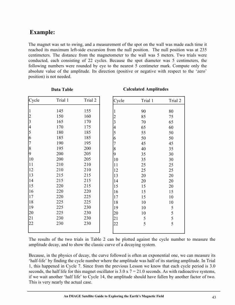
Example:
The magnet was set to swing, and a measurement of the spot on the wall was made each time itreached its maximum left-side excursion from the null position. The null position was at 235centimeters. The distance from the magnetometer to the wall was 5 meters. Two trials wereconducted, each consisting of 22 cycles. Because the spot diameter was 5 centimeters, thefollowing numbers were rounded by eye to the nearest 5 centimeter mark. Compute only theabsolute value of the amplitude. Its direction (positive or negative with respect to the ‘zero’position) is not needed.
Data Table Calculated Amplitudes
Cycle Trial 1 Trial 2
1 145 1552 150 1603 165 1704 170 1755 180 1856 185 1857 190 1958 195 2009 200 20510 200 20511 210 21012 210 21013 215 21514 215 21515 220 21516 220 22017 220 22518 225 22519 225 23020 225 23021 230 23022 230 230
Cycle Trial 1 Trial 2
1 90 802 85 753 70 654 65 605 55 506 50 507 45 458 40 359 35 3010 35 3011 25 2512 25 2513 20 2014 20 2015 15 2016 15 1517 15 1018 10 1019 10 520 10 521 5 522 5 5
The results of the two trials in Table 2 can be plotted against the cycle number to measure theamplitude decay, and to show the classic curve of a decaying system.
Because, in the physics of decay, the curve followed is often an exponential one, we can measure its‘half-life’ by finding the cycle number where the amplitude was half of its starting amplitude. In Trial1, this happened in Cycle 7. Since from the previous Lesson we know that each cycle period is 3.0seconds, the half life for this magnet oscillator is 3.0 x 7 = 21.0 seconds. As with radioactive systems,if we wait another ‘half life’ to Cycle 14, the amplitude should have fallen by another factor of two.This is very nearly the actual case.
An IMAGE Satellite Guide to Exploring the Earth’s Magnetic Field 44
Introduction:
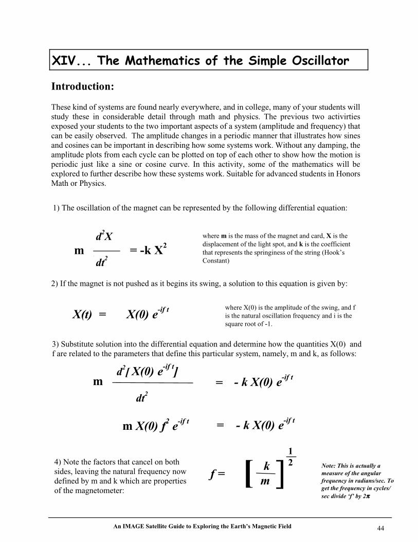
These kind of systems are found nearly everywhere, and in college, many of your students willstudy these in considerable detail through math and physics. The previous two activirtiesexposed your students to the two important aspects of a system (amplitude and frequency) thatcan be easily observed. The amplitude changes in a periodic manner that illustrates how sinesand cosines can be important in describing how some systems work. Without any damping, theamplitude plots from each cycle can be plotted on top of each other to show how the motion isperiodic just like a sine or cosine curve. In this activity, some of the mathematics will beexplored to further describe how these systems work. Suitable for advanced students in HonorsMath or Physics.
1) The oscillation of the magnet can be represented by the following differential equation:
2) If the magnet is not pushed as it begins its swing, a solution to this equation is given by:
X(t) =
where m is the mass of the magnet and card, X is thedisplacement of the light spot, and k is the coefficientthat represents the springiness of the string (Hook’sConstant)
3) Substitute solution into the differential equation and determine how the quantities X(0) andf are related to the parameters that define this particular system, namely, m and k, as follows:
m
d2[ X(0) e-if t]
dt2
= -k X2
m
m X(0) f2 e-if t
= - k X(0) e-if t
= - k X(0) e-if t
4) Note the factors that cancel on bothsides, leaving the natural frequency nowdefined by m and k which are propertiesof the magnetometer:
km
where X(0) is the amplitude of the swing, and fis the natural oscillation frequency and i is thesquare root of -1.
f = [ ]12
d2X
dt2
X(0) e-if t
Note: This is actually ameasure of the angularfrequency in radians/sec. Toget the frequency in cycles/sec divide ‘f’ by 2ππππ
An IMAGE Satellite Guide to Exploring the Earth’s Magnetic Field 45
Plotting Activity:
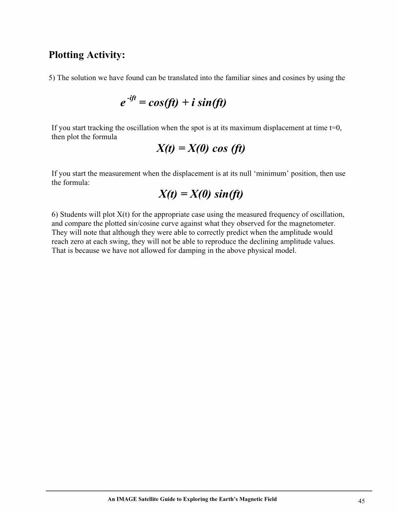
5) The solution we have found can be translated into the familiar sines and cosines by using the
e -ift = cos(ft) + i sin(ft)
If you start tracking the oscillation when the spot is at its maximum displacement at time t=0,then plot the formula
X(t) = X(0) cos (ft)
If you start the measurement when the displacement is at its null ‘minimum’ position, then usethe formula:
X(t) = X(0) sin(ft)
6) Students will plot X(t) for the appropriate case using the measured frequency of oscillation,and compare the plotted sin/cosine curve against what they observed for the magnetometer.They will note that although they were able to correctly predict when the amplitude wouldreach zero at each swing, they will not be able to reproduce the declining amplitude values.That is because we have not allowed for damping in the above physical model.
An IMAGE Satellite Guide to Exploring the Earth’s Magnetic Field 46
Including Damping in our Physical Model
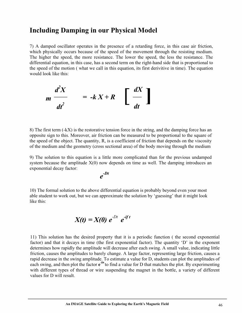
7) A damped oscillator operates in the presence of a retarding force, in this case air friction,which physically occurs because of the speed of the movement through the resisting medium.The higher the speed, the more resistance. The lower the speed, the less the resistance. Thedifferential equation, in this case, has a second term on the right-hand side that is proportional tothe speed of the motion ( what we call in this equation, its first derivitive in time). The equationwould look like this:
d2Xm dt2
= -k X + RdX
dt[ ]
8) The first term (-kX) is the restorative tension force in the string, and the damping force has anopposite sign to this. Moreover, air friction can be measured to be proportional to the square ofthe speed of the object. The quantity, R, is a coefficient of friction that depends on the viscosityof the medium and the geometry (cross sectional area) of the body moving through the medium
9) The solution to this equation is a little more complicated than for the previous undampedsystem because the amplitude X(0) now depends on time as well. The damping introduces anexponential decay factor:
10) The formal solution to the above differential equation is probably beyond even your mostable student to work out, but we can approximate the solution by ‘guessing’ that it might looklike this:
e-Dt
X(t) = X(0) e-Dt e-if t
11) This solution has the desired property that it is a periodic function ( the second exponentialfactor) and that it decays in time (the first exponential factor). The quantity ‘D’ in the exponentdetermines how rapidly the amplitude will decrease after each swing. A small value, indicating littlefriction, causes the amplitudes to barely change. A large factor, representing large friction, causes arapid decrease in the swing amplitude. To estimate a value for D, students can plot the amplitudes ofeach swing, and then plot the factor e-Dt to find a value for D that matches the plot. By experimentingwith different types of thread or wire suspending the magnet in the bottle, a variety of differentvalues for D will result.
An IMAGE Satellite Guide to Exploring the Earth’s Magnetic Field 47
Materials:
1) The Magnetometer2) A 6-10 pound container of
iron nails or the equivalent
Procedure:The magnet on the card will sense the iron mass asit is moved closer and closer to the soda bottle. Thiswill cause a deflection of the light spot on the wall.Measure the location of the light spot and plot itsdeflection from the null position against thedistance between the magnet and the iron mass.
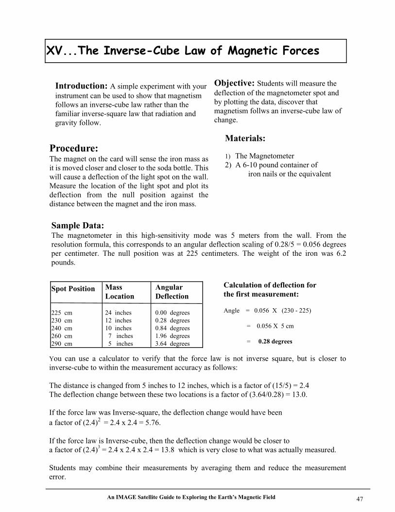
Sample Data:The magnetometer in this high-sensitivity mode was 5 meters from the wall. From theresolution formula, this corresponds to an angular deflection scaling of 0.28/5 = 0.056 degreesper centimeter. The null position was at 225 centimeters. The weight of the iron was 6.2pounds.
Spot Position
225 cm230 cm240 cm260 cm290 cm
MassLocation
24 inches12 inches10 inches 7 inches 5 inches
AngularDeflection
0.00 degrees0.28 degrees0.84 degrees1.96 degrees3.64 degrees
Calculation of deflection forthe first measurement:
Angle = 0.056 X (230 - 225)
= 0.056 X 5 cm
= 0.28 degrees
You can use a calculator to verify that the force law is not inverse square, but is closer toinverse-cube to within the measurement accuracy as follows:
The distance is changed from 5 inches to 12 inches, which is a factor of (15/5) = 2.4The deflection change between these two locations is a factor of (3.64/0.28) = 13.0.
If the force law was Inverse-square, the deflection change would have beena factor of (2.4)2 = 2.4 x 2.4 = 5.76.
If the force law is Inverse-cube, then the deflection change would be closer toa factor of (2.4)3 = 2.4 x 2.4 x 2.4 = 13.8 which is very close to what was actually measured.
Students may combine their measurements by averaging them and reduce the measurementerror.
Introduction: A simple experiment with yourinstrument can be used to show that magnetismfollows an inverse-cube law rather than thefamiliar inverse-square law that radiation andgravity follow.
Objective: Students will measure thedeflection of the magnetometer spot andby plotting the data, discover thatmagnetism follws an inverse-cube law ofchange.
An IMAGE Satellite Guide to Exploring the Earth’s Magnetic Field 48
Objective
MaterialsProcedure
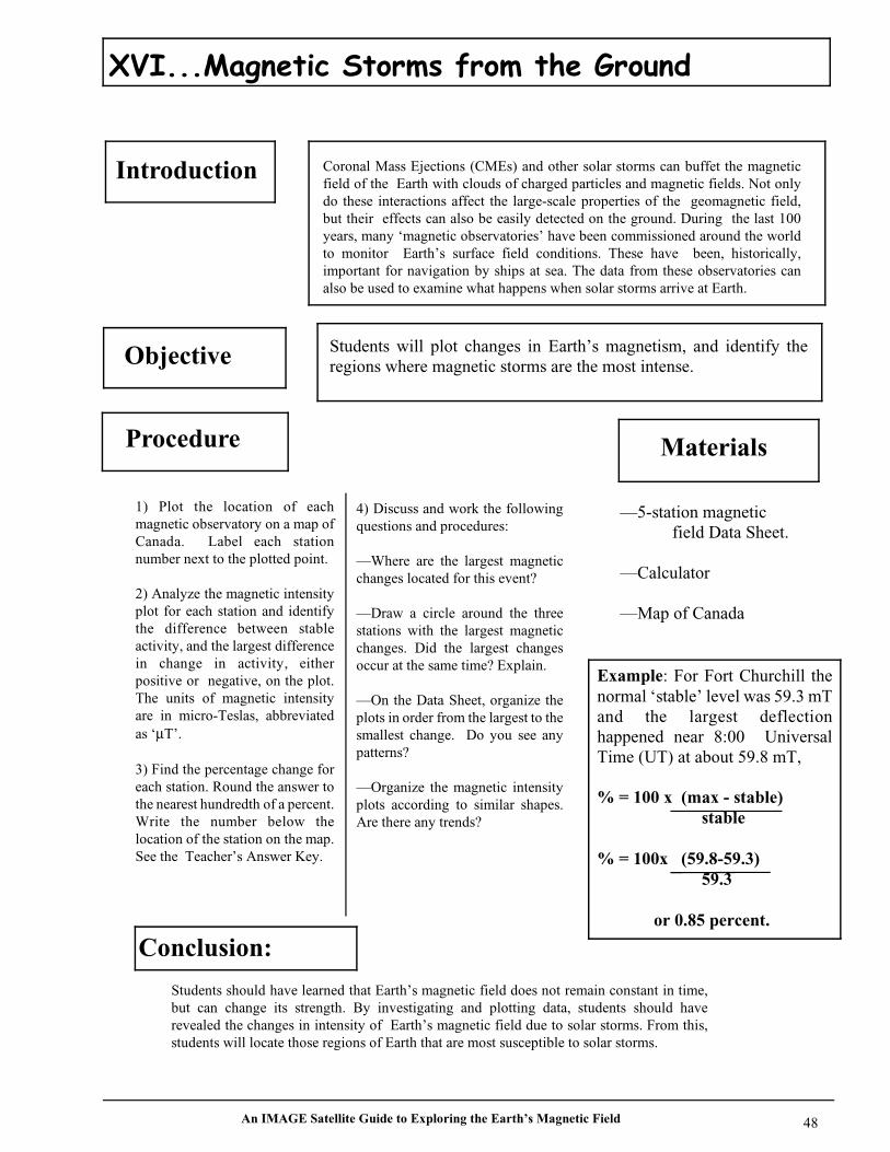
Students will plot changes in Earth’s magnetism, and identify theregions where magnetic storms are the most intense.
—5-station magnetic field Data Sheet.
—Calculator
—Map of Canada
Coronal Mass Ejections (CMEs) and other solar storms can buffet the magneticfield of the Earth with clouds of charged particles and magnetic fields. Not onlydo these interactions affect the large-scale properties of the geomagnetic field,but their effects can also be easily detected on the ground. During the last 100years, many ‘magnetic observatories’ have been commissioned around the worldto monitor Earth’s surface field conditions. These have been, historically,important for navigation by ships at sea. The data from these observatories canalso be used to examine what happens when solar storms arrive at Earth.
1) Plot the location of eachmagnetic observatory on a map ofCanada. Label each stationnumber next to the plotted point.
2) Analyze the magnetic intensityplot for each station and identifythe difference between stableactivity, and the largest differencein change in activity, eitherpositive or negative, on the plot.The units of magnetic intensityare in micro-Teslas, abbreviatedas ‘µT’.
3) Find the percentage change foreach station. Round the answer tothe nearest hundredth of a percent.Write the number below thelocation of the station on the map.See the Teacher’s Answer Key.
4) Discuss and work the followingquestions and procedures:
—Where are the largest magneticchanges located for this event?
—Draw a circle around the threestations with the largest magneticchanges. Did the largest changesoccur at the same time? Explain.
—On the Data Sheet, organize theplots in order from the largest to thesmallest change. Do you see anypatterns?
—Organize the magnetic intensityplots according to similar shapes.Are there any trends?
Conclusion:
Students should have learned that Earth’s magnetic field does not remain constant in time,but can change its strength. By investigating and plotting data, students should haverevealed the changes in intensity of Earth’s magnetic field due to solar storms. From this,students will locate those regions of Earth that are most susceptible to solar storms.
Introduction
Example: For Fort Churchill thenormal ‘stable’ level was 59.3 mTand the largest deflectionhappened near 8:00 UniversalTime (UT) at about 59.8 mT,
% = 100 x (max - stable)stable
% = 100x (59.8-59.3)59.3
or 0.85 percent.
An IMAGE Satellite Guide to Exploring the Earth’s Magnetic Field 49
60
59
52
51
58
57
60
59
58
57
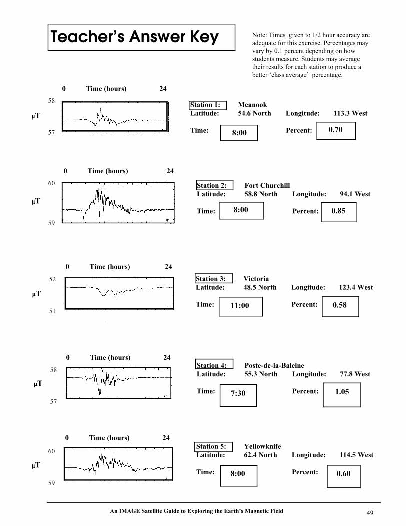
Station 1: MeanookLatitude: 54.6 North Longitude: 113.3 West
Time: Percent:
Station 2: Fort ChurchillLatitude: 58.8 North Longitude: 94.1 West
Time: Percent:
Station 3: VictoriaLatitude: 48.5 North Longitude: 123.4 West
Time: Percent:
Station 4: Poste-de-la-BaleineLatitude: 55.3 North Longitude: 77.8 West
Time: Percent:
Station 5: YellowknifeLatitude: 62.4 North Longitude: 114.5 West
Time: Percent:
Teacher’s Answer Key Note: Times given to 1/2 hour accuracy areadequate for this exercise. Percentages mayvary by 0.1 percent depending on howstudents measure. Students may averagetheir results for each station to produce abetter ‘class average’ percentage.
8:00 0.70
8:00 0.85
11:00 0.58
7:30 1.05
8:00 0.60
µµµµT
µµµµT
µµµµT
µµµµT
0 Time (hours) 24
0 Time (hours) 24
0 Time (hours) 24
0 Time (hours) 24
0 Time (hours) 24
µµµµT
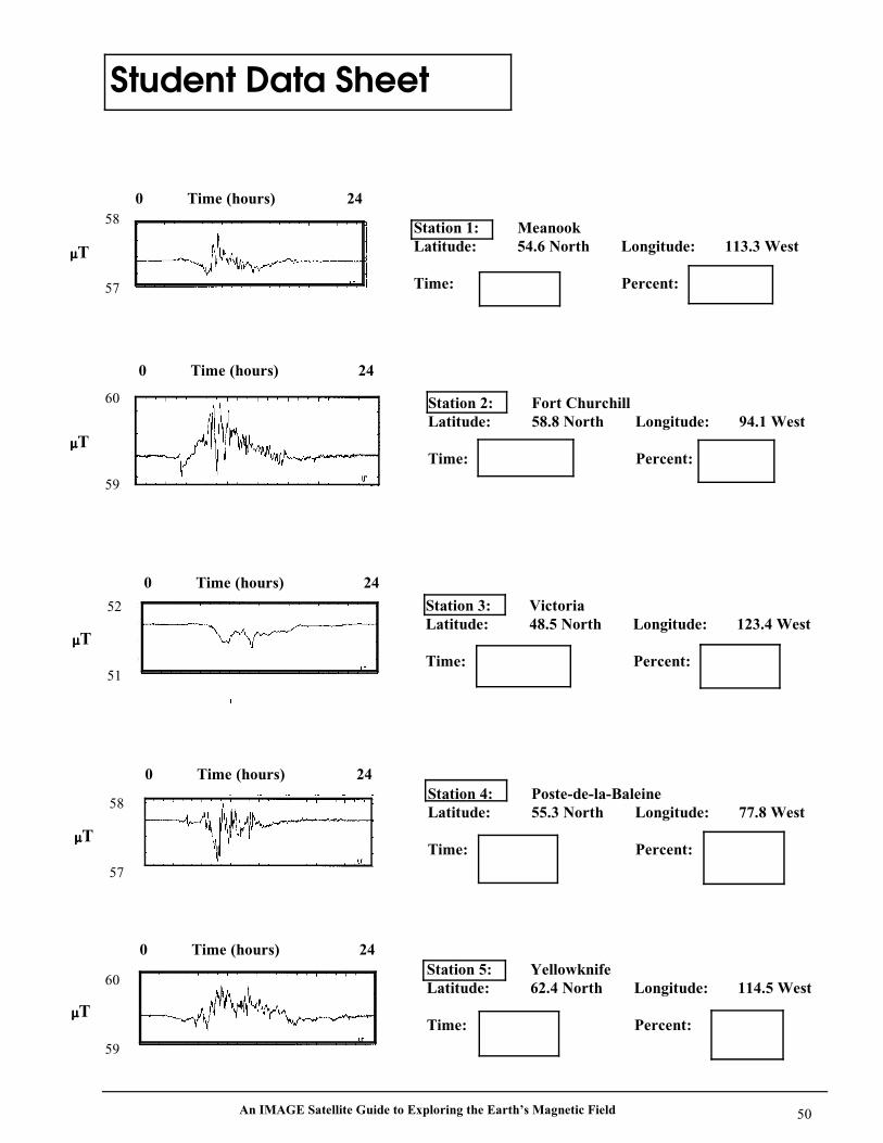
An IMAGE Satellite Guide to Exploring the Earth’s Magnetic Field 50
60
59
52
51
58
57
60
59
58
57
Station 1: MeanookLatitude: 54.6 North Longitude: 113.3 West
Time: Percent:
Station 2: Fort ChurchillLatitude: 58.8 North Longitude: 94.1 West
Time: Percent:
Station 3: VictoriaLatitude: 48.5 North Longitude: 123.4 West
Time: Percent:
Station 4: Poste-de-la-BaleineLatitude: 55.3 North Longitude: 77.8 West
Time: Percent:
Station 5: YellowknifeLatitude: 62.4 North Longitude: 114.5 West
Time: Percent:
Student Data Sheet
0 Time (hours) 24
0 Time (hours) 24
0 Time (hours) 24
0 Time (hours) 24
0 Time (hours) 24
µµµµT
µµµµT
µµµµT
µµµµT
µµµµT
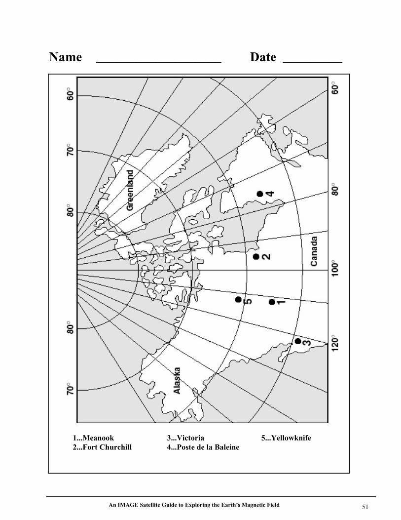
An IMAGE Satellite Guide to Exploring the Earth’s Magnetic Field 51
Name ___________________ Date _________
1...Meanook 3...Victoria 5...Yellowknife2...Fort Churchill 4...Poste de la Baleine
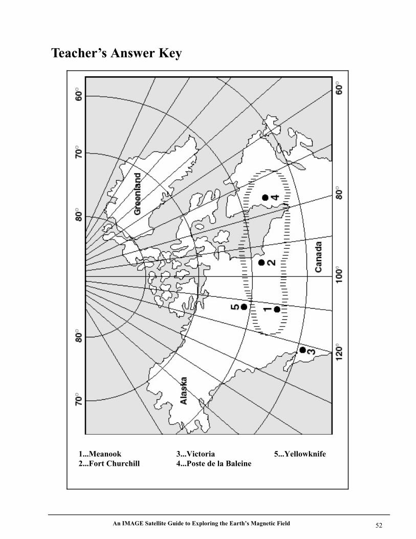
An IMAGE Satellite Guide to Exploring the Earth’s Magnetic Field 52
Teacher’s Answer Key
1...Meanook 3...Victoria 5...Yellowknife2...Fort Churchill 4...Poste de la Baleine
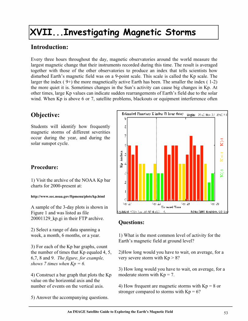
An IMAGE Satellite Guide to Exploring the Earth’s Magnetic Field 53
Introduction:
Every three hours throughout the day, magnetic observatories around the world measure thelargest magnetic change that their instruments recorded during this time. The result is averagedtogether with those of the other observatories to produce an index that tells scientists howdisturbed Earth’s magnetic field was on a 9-point scale. This scale is called the Kp scale. Thelarger the index ( 9+) the more magnetically active Earth has been. The smaller the index ( 1-2)the more quiet it is. Sometimes changes in the Sun’s activity can cause big changes in Kp. Atother times, large Kp values can indicate sudden rearrangements of Earth’s field due to the solarwind. When Kp is above 6 or 7, satellite problems, blackouts or equipment interferrence often
Objective:
Students will identify how frequentlymagnetic storms of different severitiesoccur during the year, and during thesolar sunspot cycle.
Procedure:
1) Visit the archive of the NOAA Kp barcharts for 2000-present at:
http://www.sec.noaa.gov/ftpmenu/plots/kp.html
A sample of the 3-day plots is shown inFigure 1 and was listed as file20001129_kp.gi in their FTP archive.
2) Select a range of data spanning aweek, a month, 6 months, or a year.
3) For each of the Kp bar graphs, countthe number of times that Kp equaled 4, 5,6,7, 8 and 9. The figure, for example,shows 7 times when Kp = 6.
4) Construct a bar graph that plots the Kpvalue on the horizontal axis and thenumber of events on the vertical axis.
5) Answer the accompanying questions.
Questions:
1) What is the most common level of activity for theEarth’s magnetic field at ground level?
2)How long would you have to wait, on average, for avery severe storm with Kp > 8?
3) How long would you have to wait, on average, for amoderate storm with Kp = 7.
4) How frequent are magnetic storms with Kp = 8 orstronger compared to storms with Kp = 6?
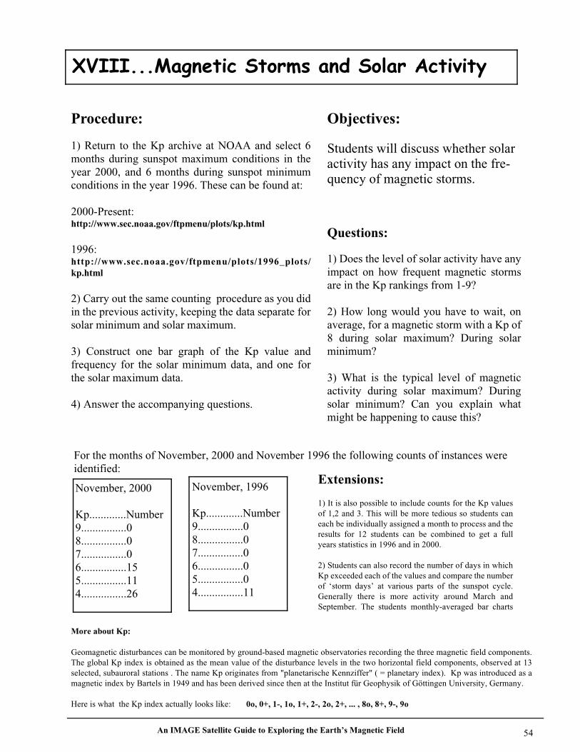
An IMAGE Satellite Guide to Exploring the Earth’s Magnetic Field 54
Procedure:
1) Return to the Kp archive at NOAA and select 6months during sunspot maximum conditions in theyear 2000, and 6 months during sunspot minimumconditions in the year 1996. These can be found at:
2000-Present:http://www.sec.noaa.gov/ftpmenu/plots/kp.html
1996:http://www.sec.noaa.gov/ftpmenu/plots/1996_plots/kp.html
2) Carry out the same counting procedure as you didin the previous activity, keeping the data separate forsolar minimum and solar maximum.
3) Construct one bar graph of the Kp value andfrequency for the solar minimum data, and one forthe solar maximum data.
4) Answer the accompanying questions.
Questions:
1) Does the level of solar activity have anyimpact on how frequent magnetic stormsare in the Kp rankings from 1-9?
2) How long would you have to wait, onaverage, for a magnetic storm with a Kp of8 during solar maximum? During solarminimum?
3) What is the typical level of magneticactivity during solar maximum? Duringsolar minimum? Can you explain whatmight be happening to cause this?
More about Kp:
Geomagnetic disturbances can be monitored by ground-based magnetic observatories recording the three magnetic field components.The global Kp index is obtained as the mean value of the disturbance levels in the two horizontal field components, observed at 13selected, subauroral stations . The name Kp originates from "planetarische Kennziffer" ( = planetary index). Kp was introduced as amagnetic index by Bartels in 1949 and has been derived since then at the Institut für Geophysik of Göttingen University, Germany.
Here is what the Kp index actually looks like: 0o, 0+, 1-, 1o, 1+, 2-, 2o, 2+, ... , 8o, 8+, 9-, 9o
For the months of November, 2000 and November 1996 the following counts of instances wereidentified:
November, 2000
Kp.............Number9................08................07................06................155................114................26
November, 1996
Kp.............Number9................08................07................06................05................04................11
Extensions:
1) It is also possible to include counts for the Kp valuesof 1,2 and 3. This will be more tedious so students caneach be individually assigned a month to process and theresults for 12 students can be combined to get a fullyears statistics in 1996 and in 2000.
2) Students can also record the number of days in whichKp exceeded each of the values and compare the numberof ‘storm days’ at various parts of the sunspot cycle.Generally there is more activity around March andSeptember. The students monthly-averaged bar charts
Objectives:
Students will discuss whether solaractivity has any impact on the fre-quency of magnetic storms.
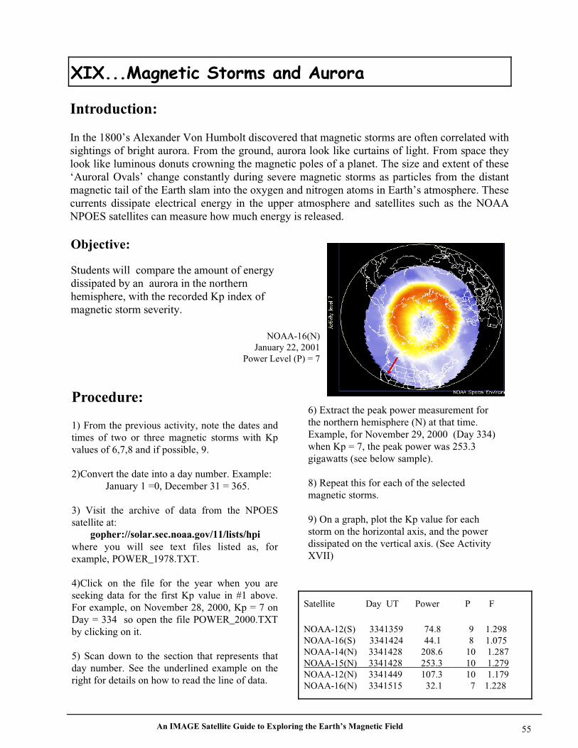
An IMAGE Satellite Guide to Exploring the Earth’s Magnetic Field 55
Introduction:
In the 1800’s Alexander Von Humbolt discovered that magnetic storms are often correlated withsightings of bright aurora. From the ground, aurora look like curtains of light. From space theylook like luminous donuts crowning the magnetic poles of a planet. The size and extent of these‘Auroral Ovals’ change constantly during severe magnetic storms as particles from the distantmagnetic tail of the Earth slam into the oxygen and nitrogen atoms in Earth’s atmosphere. Thesecurrents dissipate electrical energy in the upper atmosphere and satellites such as the NOAANPOES satellites can measure how much energy is released.
Procedure:
1) From the previous activity, note the dates andtimes of two or three magnetic storms with Kpvalues of 6,7,8 and if possible, 9.
2)Convert the date into a day number. Example: January 1 =0, December 31 = 365.
3) Visit the archive of data from the NPOESsatellite at: gopher://solar.sec.noaa.gov/11/lists/hpiwhere you will see text files listed as, forexample, POWER_1978.TXT.
4)Click on the file for the year when you areseeking data for the first Kp value in #1 above.For example, on November 28, 2000, Kp = 7 onDay = 334 so open the file POWER_2000.TXTby clicking on it.
5) Scan down to the section that represents thatday number. See the underlined example on theright for details on how to read the line of data.
Objective:
Students will compare the amount of energydissipated by an aurora in the northernhemisphere, with the recorded Kp index ofmagnetic storm severity.
NOAA-12(S) 3341359 74.8 9 1.298NOAA-16(S) 3341424 44.1 8 1.075NOAA-14(N) 3341428 208.6 10 1.287NOAA-15(N) 3341428 253.3 10 1.279 NOAA-12(N) 3341449 107.3 10 1.179NOAA-16(N) 3341515 32.1 7 1.228
Satellite Day UT Power P F
6) Extract the peak power measurement forthe northern hemisphere (N) at that time.Example, for November 29, 2000 (Day 334)when Kp = 7, the peak power was 253.3gigawatts (see below sample).
8) Repeat this for each of the selectedmagnetic storms.
9) On a graph, plot the Kp value for eachstorm on the horizontal axis, and the powerdissipated on the vertical axis. (See ActivityXVII)
NOAA-16(N)January 22, 2001
Power Level (P) = 7
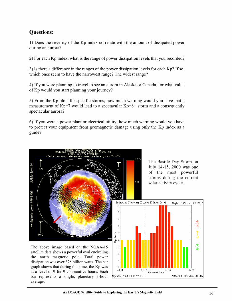
An IMAGE Satellite Guide to Exploring the Earth’s Magnetic Field 56
Questions:
1) Does the severity of the Kp index correlate with the amount of dissipated powerduring an aurora?
2) For each Kp index, what is the range of power dissipation levels that you recorded?
3) Is there a difference in the ranges of the power dissipation levels for each Kp? If so,which ones seem to have the narrowest range? The widest range?
4) If you were planning to travel to see an aurora in Alaska or Canada, for what valueof Kp would you start planning your journey?
5) From the Kp plots for specific storms, how much warning would you have that ameasurement of Kp=7 would lead to a spectacular Kp=8+ storm and a consequentlyspectacular aurora?
6) If you were a power plant or electrical utility, how much warning would you haveto protect your equipment from geomagnetic damage using only the Kp index as aguide?
The Bastile Day Storm onJuly 14-15, 2000 was oneof the most powerfulstorms during the currentsolar activity cycle.
The above image based on the NOAA-15satellite data shows a powerful oval encirclingthe north magnetic pole. Total powerdissipation was over 678 billion watts. The bargraph shows that during this time, the Kp wasat a level of 9 for 9 consecutive hours. Eachbar represents a single, planetary 3-houraverage.
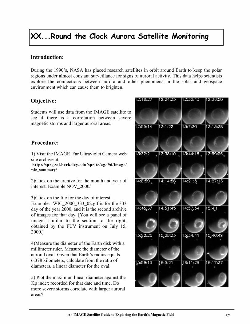
An IMAGE Satellite Guide to Exploring the Earth’s Magnetic Field 57
Introduction:
During the 1990’s, NASA has placed research satellites in orbit around Earth to keep the polarregions under almost constant surveillance for signs of auroral activity. This data helps scientistsexplore the connections between aurora and other phenomena in the solar and geospaceenvironment which can cause them to brighten.
Objective:
Students will use data from the IMAGE satellite tosee if there is a correlation between severemagnetic storms and larger auroral areas.
Procedure:
1) Visit the IMAGE, Far Ultraviolet Camera website archive at http://sprg.ssl.berkeley.edu/sprite/ago96/image/wic_summary/
2)Click on the archive for the month and year ofinterest. Example NOV_2000/
3)Click on the file for the day of interest.Example: WIC_2000_333_02.gif is for the 333day of the year 2000, and it is the second archiveof images for that day. [You will see a panel ofimages similar to the section to the right,obtained by the FUV instrument on July 15,2000.]
4)Measure the diameter of the Earth disk with amillimeter ruler. Measure the diameter of theauroral oval. Given that Earth’s radius equals6,378 kilometers, calculate from the ratio ofdiameters, a linear diameter for the oval.
5) Plot the maximum linear diameter against theKp index recorded for that date and time. Domore severe storms correlate with larger auroralareas?
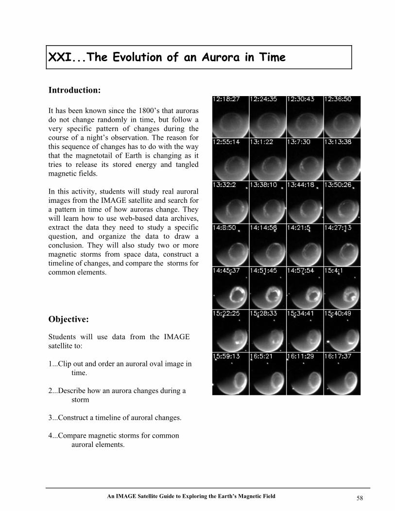
An IMAGE Satellite Guide to Exploring the Earth’s Magnetic Field 58
Introduction:
It has been known since the 1800’s that aurorasdo not change randomly in time, but follow avery specific pattern of changes during thecourse of a night’s observation. The reason forthis sequence of changes has to do with the waythat the magnetotail of Earth is changing as ittries to release its stored energy and tangledmagnetic fields.
In this activity, students will study real auroralimages from the IMAGE satellite and search fora pattern in time of how auroras change. Theywill learn how to use web-based data archives,extract the data they need to study a specificquestion, and organize the data to draw aconclusion. They will also study two or moremagnetic storms from space data, construct atimeline of changes, and compare the storms forcommon elements.
Objective:
Students will use data from the IMAGEsatellite to:
1...Clip out and order an auroral oval image in time.
2...Describe how an aurora changes during a storm
3...Construct a timeline of auroral changes.
4...Compare magnetic storms for common auroral elements.

An IMAGE Satellite Guide to Exploring the Earth’s Magnetic Field 59
Procedure:
1) Visit the IMAGE, Far Ultraviolet Camera web site archive at:
http://sprg.ssl.berkeley.edu/sprite/ago96/image/wic_summary/
2) You may either search the archive to find candidates to study, or select one of the dates belowwhich contained a strong magnetic storm event an prominent oval.
Storm Dates: November 29-31, 2000, July 14-16, 2000, June 7-10, 2000. May 223-26, 2000.
3) Click on the archive for the month and year of interest. Example NOV_2000/
4) Convert the calendar date you are interested in, into a day number for that year. Example,November 29, 2000 = day 334. [Remember to add a day for Leap Years]
5) Click on the file for the day of interest. Example: WIC_2000_333_02.gif is for the 333 dayof the year 2000, and it is the second archive (02) of images for that day. You will see a panel ofimages obtained by the FUV instrument. There may be several files to look at for that date.
6) Print out the relevant panels that show the auroral oval.
7) Clip out the individual auroral oval images being careful to note their time mark in the upperleft corner. You will use this time mark to order the picture tiles in time order.
8) On a piece of paper, order the tiles in time order, making sure to include several tiles at thebeginning and end that show little or no activity to establish a baseline for discussing thechanges.
9) Compare the ‘movie strip’ in Step 6 for at least two or three different storm events.
10) On a table that gives the elapsed time from the start of the storm ( the first picture in yourmovie will be defined as Time 0:0:0) in column 1, write an annotated description in columns 2,3 ... of what changes were seen in the oval. Some of the things you should note are, for example:
1...When did the oval reach its maximum extension towards the equator?2....When did the oval reach its maximum extension poleward?3...When did the oval reach its brightest point?4....When was the oval the thickest?5....When did the oval show the most complex interior structure?6....When did the oval show its narrowest thickness?7....When did the oval begin to fade out?
There are also other things you may see as you look very carefully at the images.
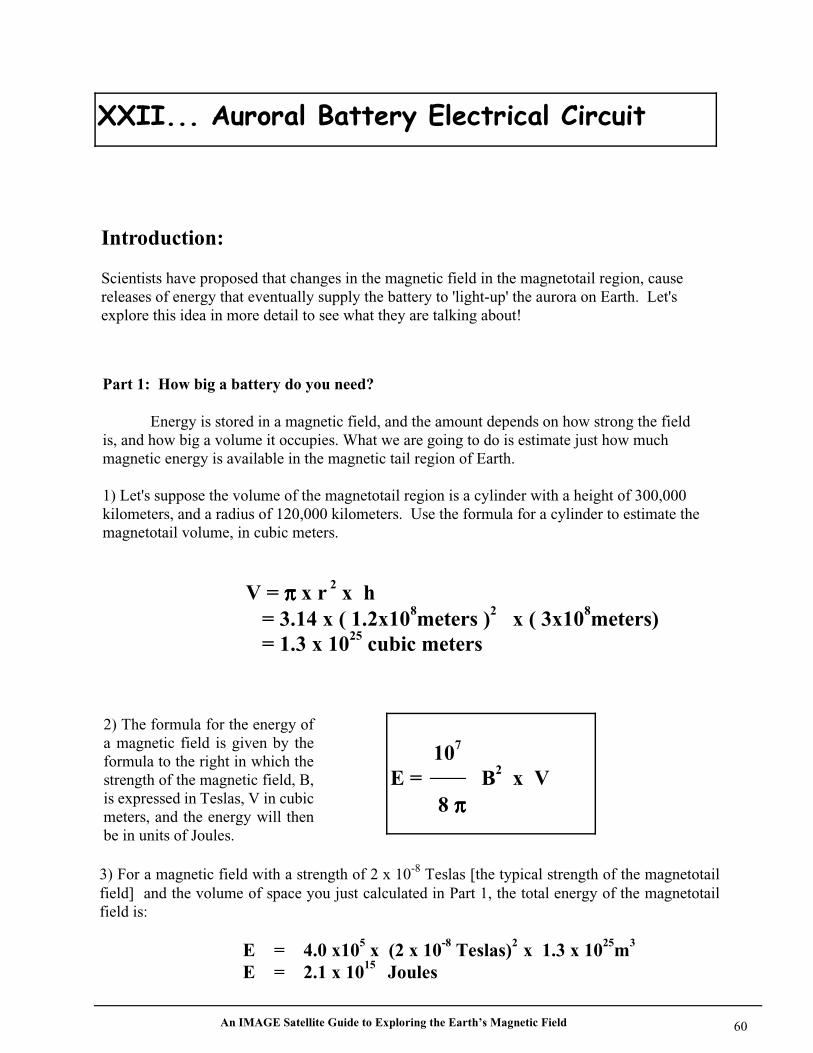
An IMAGE Satellite Guide to Exploring the Earth’s Magnetic Field 60
Introduction:
Scientists have proposed that changes in the magnetic field in the magnetotail region, causereleases of energy that eventually supply the battery to 'light-up' the aurora on Earth. Let'sexplore this idea in more detail to see what they are talking about!
Part 1: How big a battery do you need?
Energy is stored in a magnetic field, and the amount depends on how strong the fieldis, and how big a volume it occupies. What we are going to do is estimate just how muchmagnetic energy is available in the magnetic tail region of Earth.
1) Let's suppose the volume of the magnetotail region is a cylinder with a height of 300,000kilometers, and a radius of 120,000 kilometers. Use the formula for a cylinder to estimate themagnetotail volume, in cubic meters.
V = π π π π x r 2 x h = 3.14 x ( 1.2x10⁸meters )2 x ( 3x10⁸meters) = 1.3 x 1025 cubic meters
107
E = B2 x V 8 ππππ
2) The formula for the energy ofa magnetic field is given by theformula to the right in which thestrength of the magnetic field, B,is expressed in Teslas, V in cubicmeters, and the energy will thenbe in units of Joules.
3) For a magnetic field with a strength of 2 x 10⁻⁸ Teslas [the typical strength of the magnetotailfield] and the volume of space you just calculated in Part 1, the total energy of the magnetotailfield is:
E = 4.0 x105 x (2 x 10-8 Teslas)2 x 1.3 x 1025m3
E = 2.1 x 10¹⁵ Joules
An IMAGE Satellite Guide to Exploring the Earth’s Magnetic Field 61
Part 3: How many seconds can the magnetotail 'battery' continue to supplyenergy to the aurora to keep them going?
The answer to the first question in Part 1 tells us how much energy is available. The answer tothe second question tells us at what rate (energy per second) the aurora are converting energyinto light and heat.
1) To find out how long this can continue, divide the answer from question one, by the answerfrom question two:
2.1 x 10¹⁵ Joules Time =
1011 Joules/second
= 21,000 seconds, or about 5.8 hours
Although this is only an estimate, it comes very close to the most intense phase of an auroraldisplay which often lasts an entire evening. There have been many approximations used in this“back of the envelope” calculation. Have your students identify them and consider other values.Which ones might be the most uncertain? (Example: dimensions of magnetotail region involvedin the conversion of magnetic energy to particle energy, or the amperage of the auroral current.)
Part 2: How much energy do you need to light-up the auroras in theNorthern and Southern Hemispheres?
Auroras are powered by currents of electrons with currents of about 1,000,000 Amperes. Yourhome uses about 200 Amperes at 110 Volts. The atmosphere that this auroral current has to flowthrough has a resistance of about 0.1 Ohms.
Electrical power is calculated using a formula that relates resistance (R) and current (I) to thepower (P) that they can produce in a circuit:
P = I2 x R Watts
where R is measured in Ohms, and I is in Amperes. From the information given and the powerformula, you can calculate the power dissipated by an aurora:
P = ( 106 Amperes)2 x 0.1 Ohms
P = 1011 Joules/second
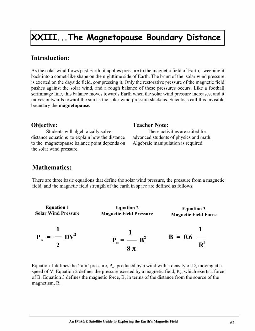
An IMAGE Satellite Guide to Exploring the Earth’s Magnetic Field 62
Introduction:
As the solar wind flows past Earth, it applies pressure to the magnetic field of Earth, sweeping itback into a comet-like shape on the nighttime side of Earth. The brunt of the solar wind pressureis exerted on the dayside field, compressing it. Only the restorative pressure of the magnetic fieldpushes against the solar wind, and a rough balance of these pressures occurs. Like a footballscrimmage line, this balance moves towards Earth when the solar wind pressure increases, and itmoves outwards toward the sun as the solar wind pressure slackens. Scientists call this invisibleboundary the magnetopause.
Objective:Students will algebraically solve
distance equations to explain how the distanceto the magnetopause balance point depends onthe solar wind pressure.
Teacher Note:These activities are suited for
advanced students of physics and math.Algebraic manipulation is required.
Mathematics:
There are three basic equations that define the solar wind pressure, the pressure from a magneticfield, and the magnetic field strength of the earth in space are defined as follows:
Equation 3Magnetic Field Force
1B = 0.6
R3
Equation 1 defines the ‘ram’ pressure, Pw, produced by a wind with a density of D, moving at aspeed of V. Equation 2 defines the pressure exerted by a magnetic field, Pw, which exerts a forceof B. Equation 3 defines the magnetic force, B, in terms of the distance from the source of themagnetism, R.
Equation 2Magnetic Field Pressure
1 Pm = B2
8 π π π π
Equation 1Solar Wind Pressure
1 Pw = DV2
2
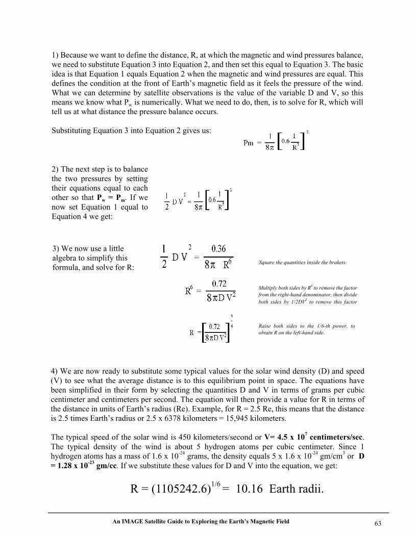
An IMAGE Satellite Guide to Exploring the Earth’s Magnetic Field 63
1) Because we want to define the distance, R, at which the magnetic and wind pressures balance,we need to substitute Equation 3 into Equation 2, and then set this equal to Equation 3. The basicidea is that Equation 1 equals Equation 2 when the magnetic and wind pressures are equal. Thisdefines the condition at the front of Earth’s magnetic field as it feels the pressure of the wind.What we can determine by satellite observations is the value of the variable D and V, so thismeans we know what Pw is numerically. What we need to do, then, is to solve for R, which willtell us at what distance the pressure balance occurs.
Substituting Equation 3 into Equation 2 gives us:
2) The next step is to balancethe two pressures by settingtheir equations equal to eachother so that Pw = Pm. If wenow set Equation 1 equal toEquation 4 we get:
3) We now use a littlealgebra to simplify thisformula, and solve for R:
Square the quantities inside the brakets.
Multiply both sides by R6 to remove the factorfrom the right-hand denominator, then divideboth sides by 1/2DV2 to remove this factor
Raise both sides to the 1/6-th power, toobtain R on the left-hand side.
4) We are now ready to substitute some typical values for the solar wind density (D) and speed(V) to see what the average distance is to this equilibrium point in space. The equations havebeen simplified in their form by selecting the quantities D and V in terms of grams per cubiccentimeter and centimeters per second. The equation will then provide a value for R in terms ofthe distance in units of Earth’s radius (Re). Example, for R = 2.5 Re, this means that the distanceis 2.5 times Earth’s radius or 2.5 x 6378 kilometers = 15,945 kilometers.
The typical speed of the solar wind is 450 kilometers/second or V= 4.5 x 10⁷ centimeters/sec.The typical density of the wind is about 5 hydrogen atoms per cubic centimeter. Since 1hydrogen atoms has a mass of 1.6 x 10⁻²⁴ grams, the density equals 5 x 1.6 x 10-24 gm/cm3 or D= 1.28 x 10⁻²³ gm/cc. If we substitute these values for D and V into the equation, we get:
R = (1105242.6)1/6 = 10.16 Earth radii.
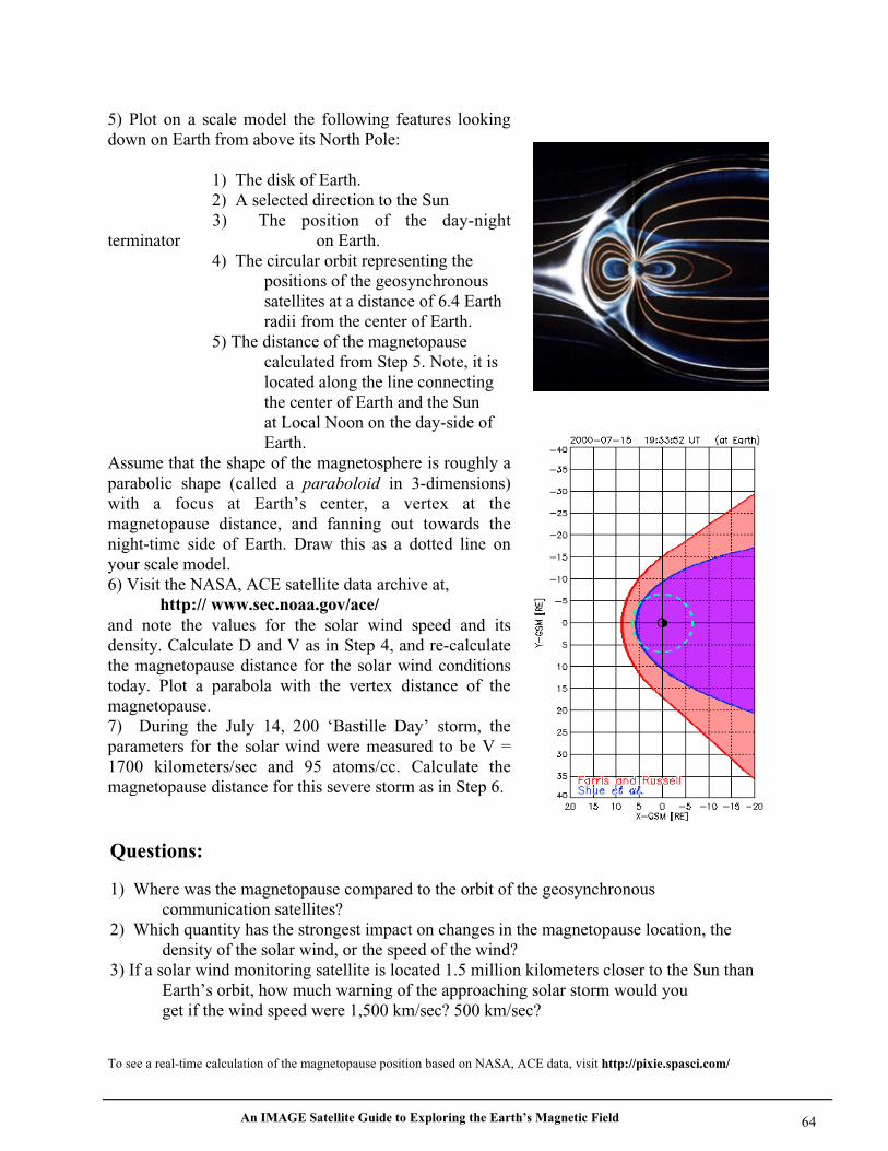
An IMAGE Satellite Guide to Exploring the Earth’s Magnetic Field 64
5) Plot on a scale model the following features lookingdown on Earth from above its North Pole:
1) The disk of Earth.2) A selected direction to the Sun3) The position of the day-night
terminator on Earth.4) The circular orbit representing the
positions of the geosynchronous satellites at a distance of 6.4 Earth radii from the center of Earth.
5) The distance of the magnetopause calculated from Step 5. Note, it is located along the line connecting the center of Earth and the Sun at Local Noon on the day-side of Earth.
Assume that the shape of the magnetosphere is roughly aparabolic shape (called a paraboloid in 3-dimensions)with a focus at Earth’s center, a vertex at themagnetopause distance, and fanning out towards thenight-time side of Earth. Draw this as a dotted line onyour scale model.6) Visit the NASA, ACE satellite data archive at,
http:// www.sec.noaa.gov/ace/and note the values for the solar wind speed and itsdensity. Calculate D and V as in Step 4, and re-calculatethe magnetopause distance for the solar wind conditionstoday. Plot a parabola with the vertex distance of themagnetopause.7) During the July 14, 200 ‘Bastille Day’ storm, theparameters for the solar wind were measured to be V =1700 kilometers/sec and 95 atoms/cc. Calculate themagnetopause distance for this severe storm as in Step 6.
To see a real-time calculation of the magnetopause position based on NASA, ACE data, visit http://pixie.spasci.com/
Questions:
1) Where was the magnetopause compared to the orbit of the geosynchronous communication satellites?
2) Which quantity has the strongest impact on changes in the magnetopause location, the density of the solar wind, or the speed of the wind?
3) If a solar wind monitoring satellite is located 1.5 million kilometers closer to the Sun than Earth’s orbit, how much warning of the approaching solar storm would youget if the wind speed were 1,500 km/sec? 500 km/sec?


![æ ò Y - WKO.at9714]-NEKP... · ï d ] o í x x x x x x x x x x x x x x x x x x x x x x x x x x x x x x x x x x x x x x x x x x x x x x x x x x x x x x x x x x x x x x x x x x x](https://img.pdfslide.net/doc/110x75/5fbaf04dd150160874293c04/-y-wkoat-9714-nekp-d-o-x-x-x-x-x-x-x-x-x-x-x-x-x-x-x-x-x-x.jpg)


![µ ] v - Casa Montessori · µ ] v 7lwoxo , x x x x x x x x x x x x x x x x x x x x x x x x x x x x x x x x x x x x x x x x x x x x x x x x x x x x x x x x x x x x x x x x x x x x](https://img.pdfslide.net/doc/110x75/5e3041645d2be568cb68ec81/-v-casa-v-7lwoxo-x-x-x-x-x-x-x-x-x-x-x-x-x-x-x-x-x-x-x-x-x-x-x-x-x.jpg)